Effect of galaxy mergers on star-formation rates
19
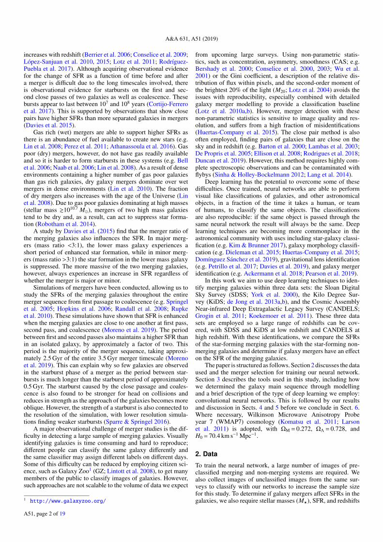
A&A 631, A51 (2019) https://doi.org/10.1051/0004-6361/201936337 c ESO 2019 Astronomy & Astrophysics Effect of galaxy mergers on star-formation rates W. J. Pearson 1,2 , L. Wang 1,2 , M. Alpaslan 3 , I. Baldry 4 , M. Bilicki 5 , M. J. I. Brown 6 , M. W. Grootes 7 , B. W. Holwerda 8 , T. D. Kitching 9 , S. Kruk 10 , and F. F. S. van der Tak 1,2 1 SRON Netherlands Institute for Space Research, Landleven 12, 9747 AD Groningen, The Netherlands e-mail: [email protected] 2 Kapteyn Astronomical Institute, University of Groningen, Postbus 800, 9700 AV Groningen, The Netherlands 3 Center for Cosmology and Particle Physics, New York University, 726 Broadway, New York, NY 10012, USA 4 Astrophysics Research Institute, Liverpool John Moores University, Twelve Quays House, Egerton Wharf, Birkenhead CH41 1LD, UK 5 Center for Theoretical Physics, Polish Academy of Sciences, Al. Lotników 32/46, 02-668 Warsaw, Poland 6 School of Physics and Astronomy, Monash University, Clayton, Victoria 3800, Australia 7 Netherlands eScience Center, Science Park 140, 1098 XG Amsterdam, The Netherlands 8 Department of Physics and Astronomy, 102 Natural Science Building, University of Louisville, Louisville, KY 40292, USA 9 Mullard Space Science Laboratory, Dorking RH5 6NT, UK 10 European Space Agency, ESTEC, Keplerlaan 1, 2201 AZ Noordwijk, The Netherlands Received 17 July 2019 / Accepted 27 August 2019 ABSTRACT Context. Galaxy mergers and interactions are an integral part of our basic understanding of how galaxies grow and evolve over time. However, the effect that galaxy mergers have on star-formation rates (SFRs) is contested, with observations of galaxy mergers showing reduced, enhanced, and highly enhanced star formation. Aims. We aim to determine the effect of galaxy mergers on the SFR of galaxies using statistically large samples of galaxies, totalling over 200 000, which is over a large redshift range from 0.0 to 4.0. Methods. We trained and used convolutional neural networks to create binary merger identifications (merger or non-merger) in the SDSS, KiDS, and CANDELS imaging surveys. We then compared the SFR, with the galaxy main sequence subtracted, of the merging and non-merging galaxies to determine what effect, if any, a galaxy merger has on SFR. Results. We find that the SFR of merging galaxies are not significantly different from the SFR of non-merging systems. The changes in the average SFR seen in the star-forming population when a galaxy is merging are small, of the order of a factor of 1.2. However, the higher the SFR is above the galaxy main sequence, the higher the fraction is for galaxy mergers. Conclusions. Galaxy mergers have little effect on the SFR of the majority of merging galaxies compared to the non-merging galaxies. The typical change in SFR is less than 0.1 dex in either direction. Larger changes in SFR can be seen but are less common. The increase in merger fraction as the distance above the galaxy main sequence increases demonstrates that galaxy mergers can induce starbursts. Key words. galaxies: interactions – galaxies: evolution – galaxies: star formation – galaxies: starburst – methods: numerical 1. Introduction Galaxy mergers and interactions form a key part of our under- standing of how galaxies form and evolve over time. In cold dark matter cosmology, dark matter halos merge under hierar- chical growth that results in the merger of the halos’ baryonic counterparts (e.g. Conselice 2014; Somerville & Davé 2015). This interaction results in the disruption of the galaxies that lie at the centre of the dark matter halos. Tidal forces act to pull and distort the galaxies, subsequently moving stars within the galaxies from the disk to the spheroid component (e.g. Toomre & Toomre 1972; Somerville & Davé 2015, and references therein). Mergers can potentially increase the activity of an active galac- tic nucleus (e.g. Sanders & Mirabel 1996; Ellison et al. 2019), although more recent work suggests this may not always be the case (e.g. Darg et al. 2010a; Weigel et al. 2018). Mergers are also thought to trigger periods of extreme star formation: starbursts. From simulations, these starbursts are believed to be a result of the tidal interactions of the galaxies that compress and shock the gas, which results in the rapid formation of stars (e.g. Barnes 2004; Kim et al. 2009; Saitoh et al. 2009). Such shock-induced star formation in mergers has also been observed (Schweizer 2009). These intense star-forming events are believed to be the cause of some of the brightest infrared objects, ultra luminous infrared galaxies (Sanders & Mirabel 1996; Niemi et al. 2012). This connection between starbursts and merging galaxies resulted in the prevailing theory that most merging galaxies go through a starburst phase (e.g. Joseph & Wright 1985; Schweizer 2005). More recent observations have shown that merger induced starbursts are found in the minority of merging systems. These studies find that the typical increase in star-formation rate (SFR) of a merger is at most a factor of two, much lower than what would typically be considered a starburst (Ellison et al. 2013; Knapen et al. 2015; Silva et al. 2018). Work by Knapen et al. (2015) shows that the majority of galaxy mergers are found to cause a reduction in the SFR when compared to non-merging galaxies of comparable stellar masses. In total, approximately 10-20% of star-forming galaxies are found to be undergoing a merger (Luo et al. 2014; Cibinel et al. 2019) while this fraction Article published by EDP Sciences A51, page 1 of 19
Transcript of Effect of galaxy mergers on star-formation rates

A&A 631, A51 (2019)https://doi.org/10.1051/0004-6361/201936337c© ESO 2019
Astronomy&Astrophysics
Effect of galaxy mergers on star-formation ratesW. J. Pearson1,2, L. Wang1,2, M. Alpaslan3, I. Baldry4, M. Bilicki5, M. J. I. Brown6, M. W. Grootes7,
B. W. Holwerda8, T. D. Kitching9, S. Kruk10, and F. F. S. van der Tak1,2
1 SRON Netherlands Institute for Space Research, Landleven 12, 9747 AD Groningen, The Netherlandse-mail: [email protected]
2 Kapteyn Astronomical Institute, University of Groningen, Postbus 800, 9700 AV Groningen, The Netherlands3 Center for Cosmology and Particle Physics, New York University, 726 Broadway, New York, NY 10012, USA4 Astrophysics Research Institute, Liverpool John Moores University, Twelve Quays House, Egerton Wharf,
Birkenhead CH41 1LD, UK5 Center for Theoretical Physics, Polish Academy of Sciences, Al. Lotników 32/46, 02-668 Warsaw, Poland6 School of Physics and Astronomy, Monash University, Clayton, Victoria 3800, Australia7 Netherlands eScience Center, Science Park 140, 1098 XG Amsterdam, The Netherlands8 Department of Physics and Astronomy, 102 Natural Science Building, University of Louisville, Louisville, KY 40292, USA9 Mullard Space Science Laboratory, Dorking RH5 6NT, UK
10 European Space Agency, ESTEC, Keplerlaan 1, 2201 AZ Noordwijk, The Netherlands
Received 17 July 2019 / Accepted 27 August 2019
ABSTRACT
Context. Galaxy mergers and interactions are an integral part of our basic understanding of how galaxies grow and evolve over time.However, the effect that galaxy mergers have on star-formation rates (SFRs) is contested, with observations of galaxy mergers showingreduced, enhanced, and highly enhanced star formation.Aims. We aim to determine the effect of galaxy mergers on the SFR of galaxies using statistically large samples of galaxies, totallingover 200 000, which is over a large redshift range from 0.0 to 4.0.Methods. We trained and used convolutional neural networks to create binary merger identifications (merger or non-merger) in theSDSS, KiDS, and CANDELS imaging surveys. We then compared the SFR, with the galaxy main sequence subtracted, of the mergingand non-merging galaxies to determine what effect, if any, a galaxy merger has on SFR.Results. We find that the SFR of merging galaxies are not significantly different from the SFR of non-merging systems. The changesin the average SFR seen in the star-forming population when a galaxy is merging are small, of the order of a factor of 1.2. However,the higher the SFR is above the galaxy main sequence, the higher the fraction is for galaxy mergers.Conclusions. Galaxy mergers have little effect on the SFR of the majority of merging galaxies compared to the non-merging galaxies.The typical change in SFR is less than 0.1 dex in either direction. Larger changes in SFR can be seen but are less common. Theincrease in merger fraction as the distance above the galaxy main sequence increases demonstrates that galaxy mergers can inducestarbursts.
Key words. galaxies: interactions – galaxies: evolution – galaxies: star formation – galaxies: starburst – methods: numerical
1. Introduction
Galaxy mergers and interactions form a key part of our under-standing of how galaxies form and evolve over time. In colddark matter cosmology, dark matter halos merge under hierar-chical growth that results in the merger of the halos’ baryoniccounterparts (e.g. Conselice 2014; Somerville & Davé 2015).This interaction results in the disruption of the galaxies that lieat the centre of the dark matter halos. Tidal forces act to pulland distort the galaxies, subsequently moving stars within thegalaxies from the disk to the spheroid component (e.g. Toomre &Toomre 1972; Somerville & Davé 2015, and references therein).Mergers can potentially increase the activity of an active galac-tic nucleus (e.g. Sanders & Mirabel 1996; Ellison et al. 2019),although more recent work suggests this may not always be thecase (e.g. Darg et al. 2010a; Weigel et al. 2018).
Mergers are also thought to trigger periods of extreme starformation: starbursts. From simulations, these starbursts arebelieved to be a result of the tidal interactions of the galaxies thatcompress and shock the gas, which results in the rapid formation
of stars (e.g. Barnes 2004; Kim et al. 2009; Saitoh et al. 2009).Such shock-induced star formation in mergers has also beenobserved (Schweizer 2009). These intense star-forming eventsare believed to be the cause of some of the brightest infraredobjects, ultra luminous infrared galaxies (Sanders & Mirabel1996; Niemi et al. 2012). This connection between starburstsand merging galaxies resulted in the prevailing theory that mostmerging galaxies go through a starburst phase (e.g. Joseph &Wright 1985; Schweizer 2005).
More recent observations have shown that merger inducedstarbursts are found in the minority of merging systems. Thesestudies find that the typical increase in star-formation rate (SFR)of a merger is at most a factor of two, much lower than whatwould typically be considered a starburst (Ellison et al. 2013;Knapen et al. 2015; Silva et al. 2018). Work by Knapen et al.(2015) shows that the majority of galaxy mergers are found tocause a reduction in the SFR when compared to non-merginggalaxies of comparable stellar masses. In total, approximately10−20% of star-forming galaxies are found to be undergoing amerger (Luo et al. 2014; Cibinel et al. 2019) while this fraction
Article published by EDP Sciences A51, page 1 of 19
A&A 631, A51 (2019)
increases with redshift (Berrier et al. 2006; Conselice et al. 2009;López-Sanjuan et al. 2010, 2015; Lotz et al. 2011; Rodríguez-Puebla et al. 2017). Although acquiring observational evidencefor the change of SFR as a function of time before and aftera merger is difficult due to the long timescales involved, thereis observational evidence for starbursts on the first and sec-ond close passes of two galaxies as well as coalescence. Thesebursts appear to last between 107 and 108 years (Cortijo-Ferreroet al. 2017). This is supported by observations that show closepairs have higher SFRs than more separated galaxies in mergers(Davies et al. 2015).
Gas rich (wet) mergers are able to support higher SFRs asthere is an abundance of fuel available to create new stars (e.g.Lin et al. 2008; Perez et al. 2011; Athanassoula et al. 2016). Gaspoor (dry) mergers, however, do not have gas readily availableand so it is harder to form starbursts in these systems (e.g. Bellet al. 2006; Naab et al. 2006; Lin et al. 2008). As a result of denseenvironments containing a higher number of gas poor galaxiesthan gas rich galaxies, dry galaxy mergers dominate over wetmergers in dense environments (Lin et al. 2010). The fractionof dry mergers also increases with the age of the Universe (Linet al. 2008). Due to gas poor galaxies dominating at high masses(stellar mass &1010.7 M), mergers of two high mass galaxiestend to be dry and, as a result, can act to suppress star forma-tion (Robotham et al. 2014).
A study by Davies et al. (2015) find that the merger ratio ofthe merging galaxies also influences the SFR. In major merg-ers (mass ratio <3:1), the lower mass galaxy experiences ashort period of enhanced star formation, while in minor merg-ers (mass ratio >3:1) the star formation in the lower mass galaxyis suppressed. The more massive of the two merging galaxies,however, always experiences an increase in SFR regardless ofwhether the merger is major or minor.
Simulations of mergers have been conducted, allowing us tostudy the SFRs of the merging galaxies throughout the entiremerger sequence from first passage to coalescence (e.g. Springelet al. 2005; Hopkins et al. 2006; Randall et al. 2008; Rupkeet al. 2010). These simulations have shown that SFR is enhancedwhen the merging galaxies are close to one another at first pass,second pass, and coalescence (Moreno et al. 2019). The periodbetween first and second passes also maintains a higher SFR thanin an isolated galaxy, by approximately a factor of two. Thisperiod is the majority of the merger sequence, taking approxi-mately 2.5 Gyr of the entire 3.5 Gyr merger timescale (Morenoet al. 2019). This can explain why so few galaxies are observedin the starburst phase of a merger as the period between star-bursts is much longer than the starburst period of approximately0.5 Gyr. The starburst caused by the close passage and coales-cence is also found to be stronger for head on collisions andreduces in strength as the approach of the galaxies becomes moreoblique. However, the strength of a starburst is also connected tothe resolution of the simulation, with lower resolution simula-tions finding weaker starbursts (Sparre & Springel 2016).
A major observational challenge of merger studies is the dif-ficulty in detecting a large sample of merging galaxies. Visuallyidentifying galaxies is time consuming and hard to reproduce;different people can classify the same galaxy differently andthe same classifier may assign different labels on different days.Some of this difficulty can be reduced by employing citizen sci-ence, such as Galaxy Zoo1 (GZ; Lintott et al. 2008), to get manymembers of the public to classify images of galaxies. However,such approaches are not scalable to the volume of data we expect
1 http://www.galaxyzoo.org/
from upcoming large surveys. Using non-parametric statis-tics, such as concentration, asymmetry, smoothness (CAS; e.g.Bershady et al. 2000; Conselice et al. 2000, 2003; Wu et al.2001) or the Gini coefficient, a description of the relative dis-tribution of flux within pixels, and the second-order moment ofthe brightest 20% of the light (M20; Lotz et al. 2004) avoids theissues with reproducibility, especially combined with detailedgalaxy merger modelling to provide a classification baseline(Lotz et al. 2010a,b). However, merger detection with thesenon-parametric statistics is sensitive to image quality and res-olution, and suffers from a high fraction of misidentifications(Huertas-Company et al. 2015). The close pair method is alsooften employed, finding pairs of galaxies that are close on thesky and in redshift (e.g. Barton et al. 2000; Lambas et al. 2003;De Propris et al. 2005; Ellison et al. 2008; Rodrigues et al. 2018;Duncan et al. 2019). However, this method requires highly com-plete spectroscopic observations and can be contaminated withflybys (Sinha & Holley-Bockelmann 2012; Lang et al. 2014).
Deep learning has the potential to overcome some of thesedifficulties. Once trained, neural networks are able to performvisual like classifications of galaxies, and other astronomicalobjects, in a fraction of the time it takes a human, or teamof humans, to classify the same objects. The classificationsare also reproducible: if the same object is passed through thesame neural network the result will always be the same. Deeplearning techniques are becoming more commonplace in theastronomical community with uses including star-galaxy classi-fication (e.g. Kim & Brunner 2017), galaxy morphology classifi-cation (e.g. Dieleman et al. 2015; Huertas-Company et al. 2015;Domínguez Sánchez et al. 2019), gravitational lens identification(e.g. Petrillo et al. 2017; Davies et al. 2019), and galaxy mergeridentification (e.g. Ackermann et al. 2018; Pearson et al. 2019).
In this work we aim to use deep learning techniques to iden-tify merging galaxies within three data sets: the Sloan DigitalSky Survey (SDSS; York et al. 2000), the Kilo Degree Sur-vey (KiDS; de Jong et al. 2013a,b), and the Cosmic AssemblyNear-infrared Deep Extragalactic Legacy Survey (CANDELS;Grogin et al. 2011; Koekemoer et al. 2011). These three datasets are employed so a large range of redshifts can be cov-ered, with SDSS and KiDS at low redshift and CANDELS athigh redshift. With these identifications, we compare the SFRsof the star-forming merging galaxies with the star-forming non-merging galaxies and determine if galaxy mergers have an effecton the SFR of the merging galaxies.
The paper is structured as follows. Section 2 discusses the dataused and the merger selection for training our neural network.Section 3 describes the tools used in this study, including howwe determined the galaxy main sequence through modellingand a brief description of the type of deep learning we employ:convolutional neural networks. This is followed by our resultsand discussion in Sects. 4 and 5 before we conclude in Sect. 6.Where necessary, Wilkinson Microwave Anisotropy Probeyear 7 (WMAP7) cosmology (Komatsu et al. 2011; Larsonet al. 2011) is adopted, with ΩM = 0.272, ΩΛ = 0.728, andH0 = 70.4 km s−1 Mpc−1.
2. Data
To train the neural network, a large number of images of pre-classified merging and non-merging systems are required. Wealso collect images of unclassified images from the same sur-veys to classify with our networks to increase the sample sizefor this study. To determine if galaxy mergers affect SFRs in thegalaxies, we also require stellar masses (M?), SFR, and redshifts
A51, page 2 of 19
W. J. Pearson et al.: Effect of galaxy mergers on star-formation rates
for the pre-classified and unclassified galaxies. We gather thesefor SDSS, KiDS, and CANDELS.
These three data sets cover different redshift ranges for whichmerger detection is attempted: the SDSS data that we use cov-ers the low redshift regime (0.005 < z ≤ 0.1), along with theKiDS data (0.00 < z ≤ 0.15), while the CANDELS data thatwe use goes to high redshift (0.0 < z ≤ 4.0). The overlaps inthe redshifts also allow us to examine differences due to res-olution, depth, and other effects, by comparing the SDSS andKiDS results, as well as different wavelengths, by comparing theoptical SDSS and KiDS with the near-infrared CANDELS. TheCANDELS data also probes rest frame optical data at z ≈ 1.2with the three CANDELS bands used (1.6 µm, 1.25 µm and814 nm) probing approximately the rest frame i, r, and g bandsused in the SDSS data.
2.1. SDSS data release 7
For the SDSS data, we use the network trained on SDSS imagesfrom Pearson et al. (2019). The merging and non-merginggalaxies used to train this network were collected followingAckermann et al. (2018). The 3003 merging galaxies are fromDarg et al. (2010a,b), itself derived from classifications fromthe Galaxy Zoo (GZ) visual classification. These galaxies haveGZ merger classification greater than 0.4 and were then visuallychecked again to ensure these galaxies are likely to be merg-ing pairs. Approximately half (54%) of these merging galax-ies are major mergers (Darg et al. 2010b), that is the ratio ofthe stellar masses of the two galaxies is less than three. Forthe non-merging galaxies, 3003 galaxies were randomly selectedfrom galaxies that have their GZ merger classification less than0.2. Cut-outs of the merging and non-merging objects werethen requested from the SDSS cut-out server for data release 72
(DR7) to create 6006 images in the gri bands, each of 256× 256pixels and with Lupton et al. (2004) colour scaling. These imageswere then cropped to the central 64× 64 pixels, correspondingto 25.3× 25.3 arcsec or 46.5× 46.5 kpc at z = 0.1, to reducememory requirements while training. The merger fraction of thecomplete training sample, before randomly selecting the non-merging galaxies but after mass completeness cuts, is ∼1.0%.
To increase the sample for analysis, all SDSS galaxies withspectroscopic redshifts between 0.005 and 0.1 were selected, tomatch the redshift range of the training sample, and were thenclassified into merging and non-merging by the Pearson et al.(2019) network, a total of 206 037 galaxies once selected formass completeness. Again, 256× 256 pixel cutouts in the gribands were collected for these galaxies from the SDSS DR7cutout server and the central 64× 64 pixels used for classifica-tion. The M? and SFR for these objects were then collected fromthe MPA-JHU catalogue3, which uses the Kroupa (2001) initialmass function (IMF; Kauffmann et al. 2003; Salim et al. 2007;Brinchmann et al. 2004). The M? is therefore derived from spec-tral energy distribution (SED) fitting while the SFR is derivedfrom Hα observations.
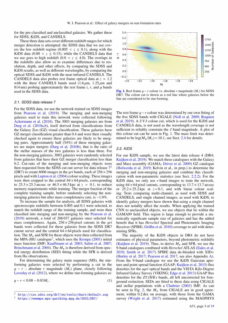
For determining the galaxy main sequence (MS), the star-forming galaxies were selected by performing a cut in theg − r – absolute r magnitude (Mr) plane, closely followingLoveday et al. (2012), where we define star-forming galaxies as:
g − r < 0.08 − 0.03Mr. (1)
2 http://cas.sdss.org/dr7/en/tools/chart/default.asp3 https://wwwmpa.mpa-garching.mpg.de/SDSS/DR7/
Fig. 1. Rest frame g − r colour vs. absolute r magnitude (Mr) for SDSSDR7. The colour cut is shown as a red line where galaxies below theline are considered to be star-forming.
The rest frame g− r colour was determined by our own fitting ofthe five SDSS bands with CIGALE (Noll et al. 2009; Boquienet al. 2019). A UV J colour cut, which is used for the KiDS andCANDELS data, is not used as the wavelength coverage is notsufficient to reliably constrain the J band magnitude. A plot ofthis colour cut can be seen in Fig. 1. The mass limit was deter-mined to be log(M?/M) = 10.1, see Sect. 2.4 for details.
2.2. KiDS
For our KiDS sample, we use the latest data release 4 (DR4;Kuijken et al. 2019). We match these catalogues with the Galaxyand Mass assembly (GAMA; Driver et al. 2009) GZ catalogue(Holwerda et al. 2019; Kelvin et al., in prep.) to determine themerging and non-merging galaxies and combine this classifi-cation with non-parametric statistics (see Sect. 2.2.2). For theKiDS data, we only use r-band images to train the network,using 64× 64 pixel cutouts, corresponding to 13.7× 13.7 arcsecor 25.2× 25.2 kpc at z = 0.1, and with linear colour scal-ing. Tests comparing multi-channel, as used with SDSS andCANDELS, and single channel images, as used with KiDS, toidentify galaxy mergers have shown that using a single channeldoes not notably affect the results. When applying the trainedCNN to unclassified objects, we use objects that lie within theGAMA09 field. This region is large enough to provide a sta-tistically significant sample size of galaxies and has the addedbenefit that it has Herschel Spectral and Photometric ImagingReceiver (SPIRE; Griffin et al. 2010) coverage to aid with deter-mining SFRs.
The majority of the KiDS objects in DR4 do not haveestimates of physical parameters, beyond photometric redshifts(Kuijken et al. 2019). Thus, to derive M? and SFR, we use the9-band catalogues combined with Herschel ATLAS (Eales et al.2010; Smith et al. 2017) SPIRE data de-blended with XID+(Hurley et al. 2017; Pearson et al. 2017, see also Appendix A).From the 9-band catalogue we use the KiDS Gaussian aper-ture and point spread function (GAAP; Kuijken et al. 2015) fluxdensities for the ugri optical bands and the VISTA Kilo-DegreeInfrared Galaxy Survey (VIKING; Edge et al. 2013) GAAP fluxdensities for the ZY JHKs bands, all left uncorrected for fore-ground extinction. SEDs are fitted to these data using CIGALEand stellar populations with a Chabrier (2003) IMF. As canbe seen in Fig. 2, the M? from CIGALE are in good agree-ment, within 0.2 dex on average, with those from the GAMAsurvey (Wright et al. 2017) estimated using the MAGPHYS
A51, page 3 of 19

A&A 631, A51 (2019)
Fig. 2. Comparison of M? from this work (y-axis) with M? from GAMA(x-axis). The red line denotes the 1-to-1 relation. The two data sets arein reasonable agreement with the average stellar masses within 0.2 dexand remain the same with and without the inclusion of SPIRE data. Thetypical statistical error on M? is 0.1 dex.
Fig. 3. Comparison of SFR from this work (y-axis) with SFR fromGAMA (x-axis). The red line denotes the 1-to-1 relation. The two datasets are within 0.2 dex on average and are consistent within the typicalerror of 0.26 dex. Both the GAMA SFRs and the SFRs from this workare derived from SED fitting.
(da Cunha et al. 2008) SED fitting tool, which also uses theChabrier (2003) IMF. A similar comparison is made with theSFR in Fig. 3, showing good agreement with GAMA.
To select the star-forming galaxies for determining the MS,a UV J colour cut was employed using the rest frame U − Vand V − J colours, determined by CIGALE during the fitting toestimate M? and SFR, and the photometric redshifts. For this,we follow Whitaker et al. (2011):
(U − V) > 0.88 × (V − J) + 0.69 z < 0.5(U − V) > 0.88 × (V − J) + 0.59 z > 0.5(U − V) > 1.3, (V − J) < 1.6 z < 1.5 (2)(U − V) > 1.3, (V − J) < 1.5 1.5 < z < 2.0(U − V) > 1.2, (V − J) < 1.4 2.0 < z < 4.0
where any galaxies that do not meet these criteria are determinedto be star-forming. An example of the colour cut is shown inFig. 4. The mass completeness limit for the KiDS galaxies wasdetermined to be log(M?/M) = 9.6, see Sect. 2.4 for details.This was determined using the magnitude limit from the GAMAsurvey of 19.8, for the r-band, as this is the limit imposed on thetraining sample.
Fig. 4. Rest frame U − V colour vs. rest frame V − J colour for KiDS.The colour cut is shown as a red line where galaxies below and to theright of the line are considered to be star-forming.
2.2.1. KiDS-GAMA Galaxy Zoo
There are no pre-existing merger catalogues for the KiDS survey,although there are visual GZ classifications for 36 706 galax-ies in the regions that overlap with the GAMA survey (KiDS-GAMA): the three GAMA equatorial fields. We can use thisclassification to help select a sample of merging galaxies touse with the KiDS data. As with other Galaxy Zoo (Lintottet al. 2008) projects, citizen scientists were asked to classifyimages of galaxies following a classification tree, as described inHolwerda et al. (2019), through the GZ web interface4 andwe use the vote fractions that are weighted for user perfor-mance. These weighted vote fractions have votes from users thatfrequently disagree with the majority of other users weightedlower, reducing their influence on the overall vote fraction. Thesegalaxies were selected to have redshifts between 0.002 and 0.15and GAMA data quality flags are used to ensure only sciencetargets are shown. Of interest here is the question concerninggalaxy interactions. This question asks the classifier to identifymerging galaxies, galaxies with tidal tails, galaxies that are bothmerging and have tidal tails or galaxies that show neither ofthese features. The latter of these classifications, galaxies thathave neither tidal tails nor show evidence of a merger, is what isused here to help identify galaxy mergers and will hence forthbe referred to as merger_neither_frac. Galaxies that havemerger_neither_frac less than 0.5, that is less than half thepeople who classified the galaxy thought it showed no tidal fea-tures or merger indications, is used here to for the basis of themerging galaxy sample with further refinements added.
2.2.2. KiDS merger selection
The visual GZ merger classifications require validation withother methods, as chance projections or star-galaxy overlaps canbe misidentified as merging galaxies (Darg et al. 2010a,b). Todo this, we use the Gini, the second-order moment of the bright-est 20% of the light (M20), concentration (C), asymmetry (A)and smoothness (S) non-parametric parameters (Lotz et al. 2004;Bershady et al. 2000; Conselice et al. 2000, 2003; Wu et al.2001). For each of the galaxies in the KiDS-GAMA sample, wederive these five non-parametric statistics using the python codestatmorph (Rodriguez-Gomez et al. 2019).
4 http://www.galaxyzoo.org/
A51, page 4 of 19
W. J. Pearson et al.: Effect of galaxy mergers on star-formation rates
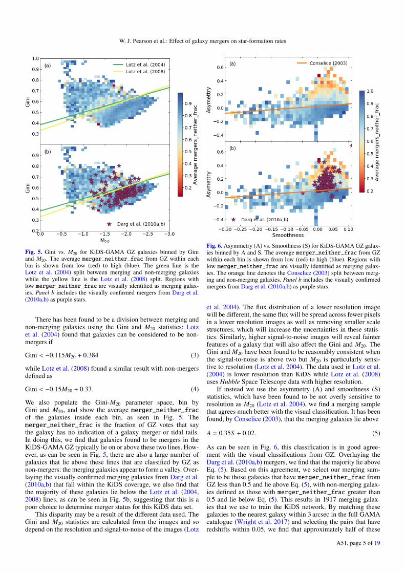
Fig. 5. Gini vs. M20 for KiDS-GAMA GZ galaxies binned by Giniand M20. The average merger_neither_frac from GZ within eachbin is shown from low (red) to high (blue). The green line is theLotz et al. (2004) split between merging and non-merging galaxieswhile the yellow line is the Lotz et al. (2008) split. Regions withlow merger_neither_frac are visually identified as merging galax-ies. Panel b includes the visually confirmed mergers from Darg et al.(2010a,b) as purple stars.
There has been found to be a division between merging andnon-merging galaxies using the Gini and M20 statistics: Lotzet al. (2004) found that galaxies can be considered to be non-mergers if
Gini < −0.115M20 + 0.384 (3)
while Lotz et al. (2008) found a similar result with non-mergersdefined as
Gini < −0.15M20 + 0.33. (4)
We also populate the Gini-M20 parameter space, bin byGini and M20, and show the average merger_neither_fracof the galaxies inside each bin, as seen in Fig. 5. Themerger_neither_frac is the fraction of GZ votes that saythe galaxy has no indication of a galaxy merger or tidal tails.In doing this, we find that galaxies found to be mergers in theKiDS-GAMA GZ typically lie on or above these two lines. How-ever, as can be seen in Fig. 5, there are also a large number ofgalaxies that lie above these lines that are classified by GZ asnon-mergers: the merging galaxies appear to form a valley. Over-laying the visually confirmed merging galaxies from Darg et al.(2010a,b) that fall within the KiDS coverage, we also find thatthe majority of these galaxies lie below the Lotz et al. (2004,2008) lines, as can be seen in Fig. 5b, suggesting that this is apoor choice to determine merger status for this KiDS data set.
This disparity may be a result of the different data used. TheGini and M20 statistics are calculated from the images and sodepend on the resolution and signal-to-noise of the images (Lotz
Fig. 6. Asymmetry (A) vs. Smoothness (S) for KiDS-GAMA GZ galax-ies binned by A and S. The average merger_neither_frac from GZwithin each bin is shown from low (red) to high (blue). Regions withlow merger_neither_frac are visually identified as merging galax-ies. The orange line denotes the Conselice (2003) split between merg-ing and non-merging galaxies. Panel b includes the visually confirmedmergers from Darg et al. (2010a,b) as purple stars.
et al. 2004). The flux distribution of a lower resolution imagewill be different, the same flux will be spread across fewer pixelsin a lower resolution images as well as removing smaller scalestructures, which will increase the uncertainties in these statis-tics. Similarly, higher signal-to-noise images will reveal fainterfeatures of a galaxy that will also affect the Gini and M20. TheGini and M20 have been found to be reasonably consistent whenthe signal-to-noise is above two but M20 is particularly sensi-tive to resolution (Lotz et al. 2004). The data used in Lotz et al.(2004) is lower resolution than KiDS while Lotz et al. (2008)uses Hubble Space Telescope data with higher resolution.
If instead we use the asymmetry (A) and smoothness (S)statistics, which have been found to be not overly sensitive toresolution as M20 (Lotz et al. 2004), we find a merging samplethat agrees much better with the visual classification. It has beenfound, by Conselice (2003), that the merging galaxies lie above
A = 0.35S + 0.02. (5)
As can be seen in Fig. 6, this classification is in good agree-ment with the visual classifications from GZ. Overlaying theDarg et al. (2010a,b) mergers, we find that the majority lie aboveEq. (5). Based on this agreement, we select our merging sam-ple to be those galaxies that have merger_neither_frac fromGZ less than 0.5 and lie above Eq. (5), with non-merging galax-ies defined as those with merger_neither_frac greater than0.5 and lie below Eq. (5). This results in 1917 merging galax-ies that we use to train the KiDS network. By matching thesegalaxies to the nearest galaxy within 3 arcsec in the full GAMAcatalogue (Wright et al. 2017) and selecting the pairs that haveredshifts within 0.05, we find that approximately half of these
A51, page 5 of 19

A&A 631, A51 (2019)
galaxies (6 of 14) are major mergers. The total number ofmatched pairs is very low, and misses pairs where the secondarygalaxy is below the magnitude limit of the survey, but this frac-tion is in line with that seen by Darg et al. (2010b) in the SDSSdata. We randomly select a further 1917 galaxies from the 20 842that lie below Eq. (5) and have merger_neither_frac greaterthan 0.5 to form the non-merging sample. With these classifica-tions for merging and non-merging galaxies, and after mass com-pleteness cuts, the merger fraction of the GZ galaxies is 8.4%.
2.3. CANDELS
To train the CANDELS network, we use the visual classi-fications for the Great Observatories Origins Deep Survey –South (GOODS-S; Giavalisco et al. 2004) from Kartaltepe et al.(2015). This catalogue contains galaxies with H magnitude lessthan 24.5 that have been classified by a small number of pro-fessional astronomers and we select objects with photometricredshift below 4.0. Of interest to this work are the classifica-tions that identify mergers (merger), interaction within a seg-mentation map (Int1), interaction with a galaxy outside of thesegmentation map (Int2), a non interacting companion (Comp)or no interaction (NoInt). During the classification, only one ofthese identifications may be chosen. The catalogue also containsan Any_Int category, which combines the merger, Int1, andInt2 identifications.
We define galaxies as merging if the Any_Int classificationis greater than 0.6 (that is more that 60% of people believe thatthe galaxy is interacting) and we define galaxies as non-mergingif the Any_Int classification is less than 0.5. As with the KiDSgalaxies, we match the merging galaxies to the rest of the CAN-DELS catalogue within 3 arcsec and selecting the pairs that haveredshifts within 0.05, we find that approximately half of thesegalaxies (4 of 9) are major mergers. Again, the total number ofmatched pairs is very low, and this method misses pairs wherethe secondary galaxy is below the magnitude limit of the sur-vey, but this fraction is in line with that seen in the SDSS data.Cutouts for these objects were created from the 1.6 µm, 1.25 µm,and 814 nm images. As the 814 nm images are twice the angu-lar resolution of the other two bands, these images are reducedin size by averaging the flux density in 2× 2 pixel groups. The1.6 µm, 1.25 µm, and 814 nm bands are then used as the red,green, and blue channels in the images, with simple linear colourscaling. As with the SDSS and KiDS images, the CANDELSimages are 64× 64 pixels, corresponding to 3.8× 3.8 arcsec or32.7× 32.7 kpc at z = 1.5. Objects with clear artefacts withinthe image were removed. This resulted in 694 merging galax-ies and we randomly select a further 694 from the 4428 non-merging galaxies that meet our criteria. The merger fraction forthe training sample using these criteria, and after mass complete-ness cuts, is 15.5%.
To increase the CANDELS sample for our analysis, weclassified all CANDELS galaxies with H-magnitude <24.5and redshift between 0.0 and 4.0, to match the training sample,from the Cosmic Evolution Survey (COSMOS; Scoville et al.2007), Extended Groth Strip (EGS; Davis et al. 2007), UKIRTInfrared Deep Sky Survey (UKIDSS) Ultra-Deep Survey (UDS;Lawrence et al. 2007; Cirasuolo et al. 2007) fields with theCANDELS network (once trained). Images for these galaxieswere created as above. The H-magnitude and SED derived SFRand M?, assuming a Chabrier (2003) IMF, come from Guoet al. (2013), Santini et al. (2015) for GOODS-S, Nayyeri et al.(2017) for COSMOS, Stefanon et al. (2017) for EGS, and Santiniet al. (2015) for UDS. As these catalogues contain a number of
Fig. 7. Rest frame U − V colour vs. rest frame V − J colour forCANDELS-z000. The colour cut is shown as a red line where galax-ies below and to the right of the line are considered to be star-forming.
different M? and SFR values, the “M_med” is used for M? and weaverage “SFR_11a_tau”, “SFR_13a_tau”, “SFR_2a_tau”, “SFR_14a”, “SFR_14a_const”, “SFR_14a_deltau”, “SFR_14a_lin”,“SFR_14a_tau”, “SFR_6a_deltau”, “SFR_6a_invtau”, and“SFR_6a_tau” for SFR, as these columns are common acrossall catalogues. These different SFR values assume differentstar-formation histories (SFH) where “cons” is a constantSFH, “tau” is an exponentially declining SFH, “deltau” is adelayed-exponential, “lin” is linearly increasing, and “inctau” isexponentially increasing. The numbers refer to the investigatorwithin the CANDELS team who lead the determination of thatSFR (Stefanon et al. 2017). For the redshift, the “z_best” value inthe catalogues were used. This value is the spectroscopic redshift,if available, or the best photometric redshift from six memberswithin the CANDELS team (Guo et al. 2013; Santini et al. 2015;Nayyeri et al. 2017; Stefanon et al. 2017).
To determine which CANDELS galaxies are star-forming,we again apply the UV J colour cuts defined in Eq. (2) usingthe rest frame U − V and V − J colours in the CANDELS cata-logues, as shown in Fig. 7. Mass completeness limits were cal-culated to be log(M?/M) = 8.3, 8.7, 9.1, 9.4, and 9.9 withinredshift bins with edges at z = 0.0, 0.6, 0.85, 1.21, 1.66, and 4.0,see also Sect. 2.4 below. These redshift bins were selected sothere are approximately 2000 galaxies within each bin after cut-ting for mass completeness. For ease of reference, these redshiftbins shall be referred to as CANDELS-z000, CANDELS-z060,CANDELS-z085, CANDELS-z121, and CANDELS-z166. Asummary of all data sets is presented in Table 1.
2.4. Mass completeness
Mass completeness limits were determined empirically by fol-lowing Pozzetti et al. (2010) and using the galaxies identified asstar-forming. For each galaxy, the mass the galaxy would need tohave to be detected at the magnitude limit (Mlim) was calculatedwith
log(Mlim) = log(M) − 0.4(xlim − x), (6)
where x is the observed magnitude in the r-band (for SDSS andKiDS) or H-band (for CANDELS) and xlim is the limiting mag-nitude of the observation. The limiting magnitudes for SDSS andCANDELS are 17.77 and 24.50 respectively. The KiDS limitingmagnitude is 19.8, the limit of the GAMA survey. The faintest20% of objects were selected and the limiting mass was the Mlimvalue that 90% of these faintest objects lie below. This was doneas a function of redshift by binning the galaxies into redshift bins
A51, page 6 of 19

W. J. Pearson et al.: Effect of galaxy mergers on star-formation rates
Table 1. Summary of data used.
Data Resolution Magnitude limit Redshift range Mass limit Training sample Complete sample(arcsec) log(M?/M) per class (Mass limited)
SDSS 1.4 17.77 0.005 < z ≤ 0.1 10.1 3003 206 037KiDS 0.77 19.8 (a) 0.00 < z ≤ 0.15 9.6 1917 1270
CANDELS-z000 0.15 24.5 0.00 < z ≤ 0.60 8.3 694 (b) 2072CANDELS-z060 0.15 24.5 0.60 < z ≤ 0.85 8.7 694 (b) 2004CANDELS-z085 0.15 24.5 0.85 < z ≤ 1.21 9.1 694 (b) 2031CANDELS-z121 0.15 24.5 1.21 < z ≤ 1.66 9.4 694 (b) 2010CANDELS-z166 0.15 24.5 1.66 < z ≤ 4.00 9.9 694 (b) 1910
Notes. The SDSS and KiDS limiting magnitudes are in r-band while the CANDELS limiting magnitude in H-band. (a)As the training set is derivedfrom GAMA classifications, the limiting magnitude is that of the GAMA survey not that of the KiDS survey. (b)The CANDELS network wastrained with 694 galaxies per class for galaxies with 0.00 < z ≤ 4.00. The galaxies were split into the redshift bins shown after classification.
as described in Sect. 4 below. These completeness limits werethen applied to the entire galaxy population.
3. Tools
3.1. Convolutional neural networksConvolutional neural networks (CNNs) are a subset of deeplearning (e.g. Lecun et al. 2015, and references therein). CNNsare used for image classifications and employ a series of non-linear mathematical functions, known as neurons, each with aweight and bias value. The structure of a CNN is built froma number of layers of these neurons. The lower layers are cre-ated from two-dimensional kernels that are convolved with theoutput of the layer below, giving CNN its name. Upper layersare one-dimensional and each neuron in these layers is con-nected to every neuron in the layer below. Forming a networkin such a way can rapidly create a large number of neurons thatrequire training resulting in many more free parameters withinthe network than there are data to train them. To reduce thisdimensionality, pooling layers are employed between the lowerconvolutional layers. These pooling layers group the inputs intoit and pass on the maximum or average value of the group,depending on the type of pooling used, with the grouping donein two-dimensions. The result is an output that is smaller in thewidth-height plane but has the same depth as the input. Theweights and biases of the neurons within a network are trained,in the case of supervised learning used here, by passing labelleddata through the network and requiring the output classificationto converge on these labels. A complete and thorough descriptionof CNNs is beyond the scope of this paper but further details areexplained in Lecun et al. (1998).
This paper uses the definitions of Pearson et al. (2019) for theterms to describe the properties of CNNs. These terms may be analternate nomenclature to other works or may be unfamiliar. Toavoid confusion we reproduce these definitions in Appendix B.
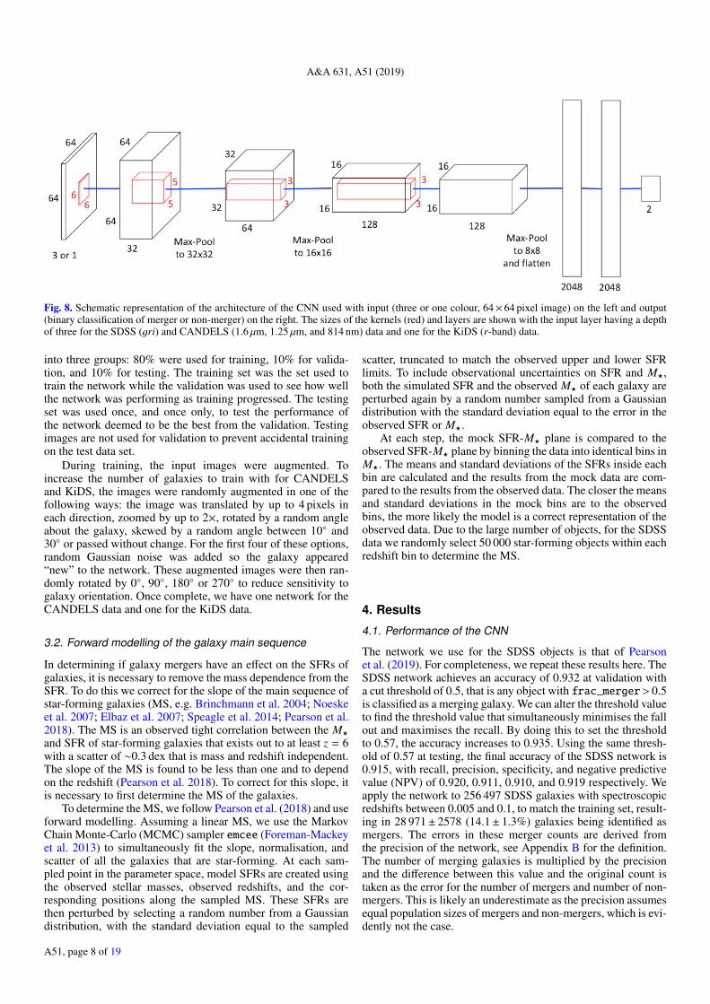
3.1.1. Architecture of the CNNFor this work, we use the architecture developed in Pearson et al.(2019) and use this to train on data from CANDELS and KiDS(the network trained in Pearson et al. 2019 is used on the SDSSimages). This network is built with Tensorflow (Abadi et al.2015) and comprises of a series of four, two-dimensional con-volutional layers followed by two one-dimensional, fully con-nected layers of 2048 neurons. The convolutional layers have32, 64, 128, and 128 kernels of 6× 6, 5× 5, 3× 3, and 3× 3 pix-els for the first, second, third, and fourth layers respectively with
the stride, how far the kernel is moved as it scans the input, setat 1 pixel for all layers and the zero padding is set to “same”to pad each edge of the image with zeros evenly (if required).2× 2 pixel max-pooling is applied after the first, second, andfourth convolutional layers to reduce the dimensionality of thenetwork. Batch normalisation (Ioffe & Szegedy 2015) is appliedafter each layer, scaling the output between zero and one, and weuse Rectified Linear Units (ReLU; Nair & Hinton 2010) for acti-vation, which returns max(x, 0) when passed x. We also applydropout (Srivastava et al. 2014) after each activation, to helpreduce over-fitting, with a dropout rate of 0.2 to randomly set theoutput of neurons to zero 20% of the time during training. Theloss of this network is determined using softmax cross entropyand optimised using the Adam algorithm (Kingma & Ba 2015)with a learning rate of 5 × 10⁻⁵. The architecture can be seenschematically in Fig. 8.
The inputs to the network are 64× 64 pixel images with eitherthree (CANDELS) or one (KiDS) colour channels, that are glob-ally scaled between 0 and 1, preserving the relative flux densitiesfor multi colour images. The output layer has two neurons, onefor each of the merging and non-merging classes, and uses a soft-max output, providing the probability for each class in the range[0, 1] that sum to unity, that is softmax maps the un-normalisedinput into it to a probability distribution over the output classesif the training, test, and validation data sets have an equal num-ber of each class. In the following, we use the output for themerger class (frac_merger) although this can be considered tobe equivalent to using the output for the non-merger class as it is1-(frac_merger) in our binary classification.
Due to the limitations of this architecture, specifically theuse of fully connected layers, it is not possible to have inputimages of different pixel sizes. As a result, it is not possible touse cutouts of different sizes that maintain the relative size of thegalaxy within the image. It is possible to resize the images butthis risks losing small scale structure when downscaling galaxiesor creating artefacts when upscaling. This may cause issues forlarge galaxies at low redshifts and low resolution as the primarygalaxy may fill the image. However, it is possible to correctlyidentify the galaxies that fill, or are larger than, the image if thetraining set contains these types of galaxies, as has been shownin Pearson et al. (2019).
3.1.2. Training, validation, and testing
If there are an unequal number of images in the two classes, thelarger class size is reduced by randomly removing images untilthe classes are the same size. The images were then subdivided
A51, page 7 of 19
A&A 631, A51 (2019)
Fig. 8. Schematic representation of the architecture of the CNN used with input (three or one colour, 64× 64 pixel image) on the left and output(binary classification of merger or non-merger) on the right. The sizes of the kernels (red) and layers are shown with the input layer having a depthof three for the SDSS (gri) and CANDELS (1.6 µm, 1.25 µm, and 814 nm) data and one for the KiDS (r-band) data.
into three groups: 80% were used for training, 10% for valida-tion, and 10% for testing. The training set was the set used totrain the network while the validation was used to see how wellthe network was performing as training progressed. The testingset was used once, and once only, to test the performance ofthe network deemed to be the best from the validation. Testingimages are not used for validation to prevent accidental trainingon the test data set.
During training, the input images were augmented. Toincrease the number of galaxies to train with for CANDELSand KiDS, the images were randomly augmented in one of thefollowing ways: the image was translated by up to 4 pixels ineach direction, zoomed by up to 2×, rotated by a random angleabout the galaxy, skewed by a random angle between 10 and30 or passed without change. For the first four of these options,random Gaussian noise was added so the galaxy appeared“new” to the network. These augmented images were then ran-domly rotated by 0, 90, 180 or 270 to reduce sensitivity togalaxy orientation. Once complete, we have one network for theCANDELS data and one for the KiDS data.
3.2. Forward modelling of the galaxy main sequence
In determining if galaxy mergers have an effect on the SFRs ofgalaxies, it is necessary to remove the mass dependence from theSFR. To do this we correct for the slope of the main sequence ofstar-forming galaxies (MS, e.g. Brinchmann et al. 2004; Noeskeet al. 2007; Elbaz et al. 2007; Speagle et al. 2014; Pearson et al.2018). The MS is an observed tight correlation between the M?
and SFR of star-forming galaxies that exists out to at least z = 6with a scatter of ∼0.3 dex that is mass and redshift independent.The slope of the MS is found to be less than one and to dependon the redshift (Pearson et al. 2018). To correct for this slope, itis necessary to first determine the MS of the galaxies.
To determine the MS, we follow Pearson et al. (2018) and useforward modelling. Assuming a linear MS, we use the MarkovChain Monte-Carlo (MCMC) sampler emcee (Foreman-Mackeyet al. 2013) to simultaneously fit the slope, normalisation, andscatter of all the galaxies that are star-forming. At each sam-pled point in the parameter space, model SFRs are created usingthe observed stellar masses, observed redshifts, and the cor-responding positions along the sampled MS. These SFRs arethen perturbed by selecting a random number from a Gaussiandistribution, with the standard deviation equal to the sampled
scatter, truncated to match the observed upper and lower SFRlimits. To include observational uncertainties on SFR and M?,both the simulated SFR and the observed M? of each galaxy areperturbed again by a random number sampled from a Gaussiandistribution with the standard deviation equal to the error in theobserved SFR or M?.
At each step, the mock SFR-M? plane is compared to theobserved SFR-M? plane by binning the data into identical bins inM?. The means and standard deviations of the SFRs inside eachbin are calculated and the results from the mock data are com-pared to the results from the observed data. The closer the meansand standard deviations in the mock bins are to the observedbins, the more likely the model is a correct representation of theobserved data. Due to the large number of objects, for the SDSSdata we randomly select 50 000 star-forming objects within eachredshift bin to determine the MS.
4. Results
4.1. Performance of the CNN
The network we use for the SDSS objects is that of Pearsonet al. (2019). For completeness, we repeat these results here. TheSDSS network achieves an accuracy of 0.932 at validation witha cut threshold of 0.5, that is any object with frac_merger> 0.5is classified as a merging galaxy. We can alter the threshold valueto find the threshold value that simultaneously minimises the fallout and maximises the recall. By doing this to set the thresholdto 0.57, the accuracy increases to 0.935. Using the same thresh-old of 0.57 at testing, the final accuracy of the SDSS network is0.915, with recall, precision, specificity, and negative predictivevalue (NPV) of 0.920, 0.911, 0.910, and 0.919 respectively. Weapply the network to 256 497 SDSS galaxies with spectroscopicredshifts between 0.005 and 0.1, to match the training set, result-ing in 28 971± 2578 (14.1± 1.3%) galaxies being identified asmergers. The errors in these merger counts are derived fromthe precision of the network, see Appendix B for the definition.The number of merging galaxies is multiplied by the precisionand the difference between this value and the original count istaken as the error for the number of mergers and number of non-mergers. This is likely an underestimate as the precision assumesequal population sizes of mergers and non-mergers, which is evi-dently not the case.
A51, page 8 of 19

W. J. Pearson et al.: Effect of galaxy mergers on star-formation rates
Table 2. Statistics for trained CNNs.
SDSS (a) KiDS CANDELS0.005 < z < 0.1 0.00 < z ≤ 0.15 0.00 < z ≤ 4.0
Cut threshold 0.57 0.52 0.47ROC area 0.966 0.957 0.861Recall 0.920 0.942 0.870Precision 0.911 0.874 0.789Specificity 0.910 0.864 0.768NPV 0.919 0.938 0.855Accuracy 0.915 0.903 0.818
Notes. Definitions of terms can be found in Appendix B. (a)The SDSSnetwork is that of Pearson et al. (2019).
For the KiDS network, we use the CNN to identify galax-ies that fall within the GAMA09 field. This network achievesan accuracy of 0.942 at validation with a cut threshold of 0.5.If we alter the threshold to 0.52, to simultaneously minimise thefall out and maximise the recall, the accuracy increases to 0.948.Using the same threshold of 0.52 at testing, the final accuracyof the KiDS network is 0.903, with recall, precision, specificity,and NPV of 0.942, 0.874, 0.864, and 0.938 respectively. Despitethe resolution of the KiDS images being higher than that of theSDSS images, the same image size resulted in the best perfor-mance for the KiDS network: 64× 64 pixels. Larger images weretried but these networks did not perform as well. Applying theKiDS network to all galaxies in the GAMA09 field with photo-metric redshifts below 0.15, a total of 1270 galaxies, we identify436± 55 (30.0± 4.3%) merging galaxies.
The CANDELS network achieves an accuracy of 0.826 atvalidation with a cut threshold of 0.5. If we decrease the thresh-old to 0.47, the accuracy increases to 0.840. Using the samethreshold of 0.47 at testing, the final accuracy of the CAN-DELS network is 0.818, with recall, precision, specificity, andNPV of 0.870, 0.789, 0.768, and 0.855 respectively. The poorerresults for the CANDELS network is likely due to fewer pre-classified objects to train the network with, 694 per class forCANDELS compared to 3003 for SDSS, as well as the higherredshifts of the training objects. The CANDELS images alsocover a much larger redshift range, resulting in a greater dis-tribution of sizes in the image for galaxies at the same massthan the SDSS images. Ideally, it would be preferable to splitthe galaxies into redshift bins and train a network per redshiftto minimise this effect, however with so few objects it is notfeasible. We apply the CANDELS network to the objects withH-magnitude <24.5 and 0.0 < z < 4.0 in the CANDELS COS-MOS, EGS, and UDS fields and identify 3535± 746 merger can-didates out of the 10 027 galaxies in these three fields. This isa merger fraction of 35.3± 7.4%, which is high. The statisticsfor all the networks are presented in Table 2 and examples ofnon-merger and mergers selected by the CNNs can be found inAppendix C.
4.2. SDSS
To determine the effect of galaxy mergers on SFR, we determinethe effect of mergers on the MS subtracted SFR. We fit the MSto all the star-forming galaxies, both mergers and non-mergerstogether, and the MS we have fitted to the SDSS data is shownoverlaid onto all the non-merging and merging galaxies in Fig. 9.The MS subtracted SFR of the merging and non-merging galax-ies are then compared by fitting a skewed Gaussian distribution,
Fig. 9. SFR-M? plane populated with (a) non-merging galaxies and(b) merging SDSS galaxies. The colour indicates the number densityfrom low (light yellow) to high (dark purple). Overlaid in red is theMS that has been fitted to all star-forming galaxies. As can be seen, thedistributions of the merging and non-merging galaxies are similar withrespect to the plotted MS.
of the form
y =Aσ
exp( (x − µ)
2σ2
)(1 + erf
[α(x − µ)√
2σ
]), (7)
to the distributions of the merging and non-merging galaxies,where A is the amplitude, µ, and σ are the mean and standarddeviation of the Gaussian, α is the description of skewness, ander f is the error function.
To fit the skewed Gaussian we bin the MS subtracted SFRwith bin sizes of 0.25 dex, between −3 log(M yr−1) and 2log(M yr−1) and fit the skewed Gaussian to the number of galax-ies in each bin. The errors on these counts were determined bygenerating 100 realisations of the MS subtracted SFR by perturb-ing the SFR and M? of each galaxy by a random number drawnfrom a Gaussian distribution centred on the observed SFR or M?
and with the error on the value as the standard deviation. Eachrealisation was then binned in the same way as the observationsand the standard deviation of the counts in the bins of the 100realisations were taken as the errors on the counts of the obser-vations. The scipy.optimize package curve_fit was thenused to fit the skewed Gaussian distribution to the counts in thebins and account for their errors. The distributions are presentedin Fig. 10 with the parameters for the skewed Gaussian fits inTable 3.
Comparing the skewed Gaussian fits to the distributions, wefind that the mean for the star-forming mergers and non-mergersare consistent within three times the error of the mean (σµ) andthe merging galaxies have higher mean MS subtracted SFR. Thissuggests that the star-forming population has a slightly, but notsignificantly, increased SFR when undergoing a merger.
A51, page 9 of 19

A&A 631, A51 (2019)
Table 3. Best fit parameters for skewed Gaussian distributions fitted tostar-forming SDSS data.
Parameter Merger Non-merger
µ 0.33± 0.02 0.25± 0.01σ 0.43± 0.02 0.39± 0.01α −1.29± 0.18 −1.52± 0.16
Notes. µ and σ are in units of log(M yr−1).
Fig. 10. Distribution of MS subtracted SFR for star-forming SDSS non-merging galaxies (blue) and merging galaxies (red). As can be seen, themerging star-forming population has a slightly higher mean MS sub-tracted SFR.
Fig. 11. Distribution of MS subtracted SFR for star-forming KiDS non-merging galaxies (blue) and merging galaxies (red). As can be seen, themerging star-forming galaxies have a similar mean MS subtracted SFRto the non-merging galaxies.
4.3. KiDS
As with the SDSS data, we fit a skewed Gaussian distribution tothe MS subtracted SFR of the star-forming galaxies. An exampleof the resulting MS subtracted SFR distributions for the KiDS isshown in Fig. 11. Table 4 shows that the merging star-forminggalaxies have higher average SFRs. The differences not large,with the mean MS subtracted SFR being within 3σµ of eachother.
Table 4. Best fit parameters for skewed Gaussian distributions fitted tostar-forming KiDS data.
Parameter Merger Non-merger
µ 0.44± 0.1 0.13± 0.18σ 0.47± 0.09 0.41± 0.08α −1.53± 0.91 −0.63± 0.78
Notes. µ and σ are in units of log(M yr−1).
Fig. 12. Distribution of MS subtracted SFR for the 0.85 < z ≤ 1.21redshift bin for CANDELS non-merging galaxies (blue) and merginggalaxies (red). This is the only data that is fitted with a double Gaussiandistribution due to the clear multi-modal population. As can be seen,the main and secondary populations have a slightly higher mean MSsubtracted SFR than the non-merging galaxies.
4.4. CANDELS
Due to the larger redshift coverage of the CANDELS data, wecan examine if the impact of galaxy mergers on SFR changes as afunction of redshift. To do this, we divided the data into redshiftbins with edges at z = 0.0, 0.6, 0.85, 1.21, 1.66, and 4.0, eachwith its own mass completeness limit and containing approxi-mately 2000 galaxies after mass completeness cuts have beenapplied. Each redshift bin also had its own main sequence fit-ted as outlined in Sect. 3.2. For ease of reference, these redshiftbins shall be referred to as CANDELS-z000, CANDELS-z060,CANDELS-z085, CANDELS-z121, and CANDELS-z166.
As before, we fit the distributions of the star-forming CAN-DELS galaxies with a skewed Gaussian function. However, thereis an indication of a second, high SFR population in CANDELS-z085 (0.85 < z ≤ 1.21), identifiable when the error on theskew of the both the merging and non-merging distributions aregreater than 104 and so in that bin only, we fit a double Gaussiandistribution and consider the lower mean to be the mean of thestar-forming population. The distributions for the MS subtractedSFR for this redshift bin is shown in Fig. 12.
Using the best fitting values for the skewed and double Gaus-sian functions presented in Table 5, in the lowest redshift binthe merging galaxies act to suppress the SFR of galaxies, withthe mean MS subtracted SFR for merging galaxies lower thannon-merging galaxies by more than 3σµ. At redshifts abovez = 0.60, the star-forming mergers have a higher mean than thestar-forming non-mergers or are consistent within 3σµ.
A51, page 10 of 19

W. J. Pearson et al.: Effect of galaxy mergers on star-formation rates
Table 5. Best fit parameters for skewed or double Gaussian distributionsfitted to star-forming CANDELS data.
Redshift Parameter Merger Non-merger
µ −0.37± 0.17 −0.27± 0.020.0 < z ≤ 0.6 σ 0.47± 0.08 0.29± 0.02
α 9999.489± 87523220.85 1.21± 0.26µ 0.10± 0.12 0.02± 0.11
0.6 < z ≤ 0.85 σ 0.24± 0.07 0.24± 0.06α −0.878± 1.17 −0.79± 0.99
0.85 < z ≤ 1.21 µ −0.12± 0.01 −0.16± 0.01σ 0.20± 0.01 0.20± 0.01µ −0.43± 0.02 −0.42± 0.02
1.21 < z ≤ 1.66 σ 0.62± 0.03 0.52± 0.03α 5.058± 1.24 3.13± 0.69µ −0.47± 0.02 −0.5± 0.02
1.66 < z ≤ 4.0 σ 0.65± 0.03 0.61± 0.03α 3.241± 0.51 3.7± 0.61
Notes. For the 0.85 < z ≤ 1.21 bin, where a double Gaussian is used,the star-forming component is the component with the lowest µ. µ, andσ are in units of log(M yr−1).
5. Discussion
Here we present discussions of our results. We note that directcomparisons between the results of the three data sets is diffi-cult due to the different definitions of mergers employed for thetraining data sets as well as difference in data quality, such asdepth and resolution, which can also influence merger identifi-cation. While the merger definitions are similar, as they are allbased on visual classification, the specifics of the definitions dif-fer. The classifications also cover both major and minor mergers,with approximately half of each training set comprising of majormergers. This likely results in a similar split for the mergers clas-sified by our networks.
5.1. Merger influence on SFR
Across the SDSS, CANDELS, and KiDS data sets there is adifference between the SFRs of the merging and non-merginggalaxies. However, the difference between the two is small andvaries between the data sets as well as within the data sets. Whatis evident is that the merging systems are not only found as star-burst galaxies but also as star-forming and quiescent systems.
Comparing the SDSS data with the KiDS data, we find littledifference in how mergers are affecting the SFR. Both data setsshow that star-forming merging galaxies have a slight increasein SFR. Within the CANDELS-z000 data the opposite is found:we find that there is a decrease in the MS subtracted SFR, sug-gesting that galaxy mergers are acting to reduce the SFR of thestar-forming galaxies. The full comparison between the aver-age SFRs for all data sets at all redshifts studied can be seenin Fig. 13.
The slight difference between the merging and non-mergingSFRs is also not a result of the observation bands or methodsused to derive the SFR. The mergers in all three surveys aredetected using different bands: SDSS uses three optical bands(gri), CANDELS uses observed frame near infrared (Hubble1.6 µm, 1.25 µm, and 814 nm bands), and KiDS uses a singleoptical band (r band). SFRs in the three surveys are also deriveddifferently: SDSS uses Hα based SFR while CANDELS andKiDS use SED derived SFR. The models used to derive theCANDELS and KiDS SFRs and M? are also different. Thus, the
Fig. 13. Average MS subtracted SFR of star-forming galaxies for SDSSmerging (purple circle) and non-merging (dark blue diamond); KiDSmerging (light blue circle) and non-merging (green diamond); andCANDELS merging (orange circles) and non-merging (red diamonds)galaxies. As can be seen, the change in SFR between the merging andnon-merging galaxies is typically small.
small effect of merging galaxies on the SFRs seen is this studyis robust.
Our results are qualitatively in line with previous work inthat we only find small (less than a factor of two) changes inSFR. Lackner et al. (2014) and Knapen et al. (2015) find thatmergers change the SFR by up to a factor of two. While we donot find that mergers always result in an increase in SFR, we dofind that the change in SFR caused by a galaxy merger is typi-cally small over the timescale of the entire merger. If an increasein SFR due to a galaxy merger is large but shorter lived, the effectwill be hidden by the larger number of galaxies not undergoingsuch a burst of star formation. The changes in average MS sub-tracted SFR are small and typically found to be a factor of ∼1.2.Similarly, Silva et al. (2018) find that mergers produce no sig-nificant change to the SFR of galaxies, which is consistent withthe results of our study. However, caution must be taken withthis comparison as the work of Silva et al. (2018) uses merg-ers where the two merging galaxies are within 3−15 kpc of eachother, something that this work does not take into account.
This study has its limitations. It is likely that we are observ-ing different stages of galaxy mergers but our method is cur-rently unable to determine at what stage the mergers are. As aresult, it is not possible to say, from this study, if mergers causea migrating of the merging galaxies across the SFR-M? plane orif the merger only slightly affects the SFR resulting in the smallchanges we observe.
5.2. Merger fractions
The merger fractions for CANDELS, 35.3± 7.4%, and KiDS,36.9± 5.3%, are notably higher than the merger fractions for theSDSS data at 14.1± 1.3%, see Table 6 and Figs. 14 and 15. Theerrors in these merger fractions are derived from the precisionof the network, see Appendix B for the definition. The numberof merging galaxies is multiplied by the precision and the dif-ference between this value and the original count is taken as theerror for the number of mergers and number of non-mergers. Themerging fraction for the precision corrected counts is then cal-culated and the difference between the original fraction and thisprecision corrected fraction is taken as the error. This is likely an
A51, page 11 of 19

A&A 631, A51 (2019)
Table 6. Merger fraction by redshift and data set for quiescent, star-forming, and total galaxy populations.
Data set Total Quiescent Star-forming
SDSS 14.1± 1.3% 14.3± 1.3% 13.4± 1.2%KiDS 30.0± 4.3% 19.4± 2.8% 36.9± 5.3%CANDELS-z000 32.0± 6.8% 30.0± 6.2% 32.4± 6.8%CANDELS-z060 32.2± 6.8% 20.2± 4.3% 33.6± 7.1%CANDELS-z085 32.6± 6.9% 24.4± 5.1% 33.3± 7.0%CANDELS-z121 37.8± 8.0% 23.9± 5.3% 39.4± 8.3%CANDELS-z166 42.1± 8.9% 28.5± 5.9% 44.3± 9.3%
Notes. Errors are derived from correcting for the precision of thenetwork.
Fig. 14. Total merger fraction as a function of redshift for SDSS (darkblue circle), KiDS (light blue circle), and CANDELS (red circles) byredshift bin. Also plotted are the mass limited merger fractions withlog(M?/M)> 10.0 from Conselice et al. (2003, green stars), Cotiniet al. (2013, lilac diamonds), Lotz et al. (2011) magnitude limitedmerger fractions with MB > −19.2 (orange crosses), and the Duncanet al. (2019) lower mass (9.7< log(M?/M < 10.3, L, purple left tri-angles) and higher mass (log(M?/M > 10.3, H, brown right trian-gles) merger fractions. The SDSS data are slightly higher than wouldbe expected and the KiDS and CANDELS merger fractions are approx-imately a factor of two higher than the other results.
underestimate as the precision assumes equal population sizes ofmergers and non-mergers, which is evidently not the case.
Even only considering the lowest redshift bin for CAN-DELS, 0.00 < z ≤ 0.60, the merger fraction is much higher thanthe SDSS and higher redshift KiDS at 32.0± 6.8%. It is unsur-prising that this becomes a larger issue as the redshift increasesbecause the pixel size of the galaxy within the image becomessmaller and the galaxies themselves become fainter, suppressingthe features that the CNN looks for to identify a merging galaxy.
Comparing our merger fractions to other works shows thatthe CANDELS results are indeed much higher than would beexpected. Figure 14 shows the comparison of this work withConselice et al. (2003), who use CAS to identify mergers, Lotzet al. (2011), who use Gini and M20, Cotini et al. (2013), who useCAS, Gini and M20, and Duncan et al. (2019), who use the closepair method. The results of Duncan et al. (2019) are the mergerpair fraction (the number of pairs of merging galaxies dividedby the total number of galaxies) and so we multiply their valuesby 0.6 to compare to our results (Lotz et al. 2011; Mundy et al.2017).
Fig. 15. Merger fraction of quiescent (diamonds) and star-forming (cir-cles) as a function of redshift for SDSS (purple and blue), KiDS (yel-low and green), and CANDELS (orange and red). There is no overalltrend with redshift with SDSS having a lower merger fraction for thestar-forming galaxies, KiDS having a higher merger fraction for star-forming galaxies, and CANDELS star-forming galaxies having a highermerger fraction at all redshifts.
The SDSS merger fraction is higher than the other works inthe same redshift range but is consistent with the merger frac-tions of Conselice et al. (2003) and Lotz et al. (2011) at higherredshifts. The KiDS data has a merger fraction that is highercompared to the other works, both at similar and higher red-shifts, similar to the merger fractions from CANDELS as dis-cussed above.
We can compare the merger fractions of the quiescent andstar-forming galaxies as shown in Fig. 15. The SDSS data has aslightly lower merger fraction for the quiescent galaxies than thestar-forming galaxies, although the difference is 0.2 percentagepoints, much less than the error on the merger fractions. KiDSdata has a higher merger fraction for the quiescent galaxies thanthe star-forming galaxies. As these two data sets cover simi-lar redshift ranges one would expect to see a similar trend inthe merger fractions of these two populations. The difference inoverall merger fractions may be a result of the SDSS and KiDSnetworks not being identical and the different selection criteriafor the training sets.
This is qualitatively different to the CANDELS-z000 datathat has a slightly lower quiescent merger fraction than star-forming merger fraction. This difference is more pronounced athigher redshifts resulting in a different conclusion from the KiDSdata. The CANDELS data suggests that there is a higher fractionof star-forming galaxy mergers than quiescent galaxy mergers atall redshifts, implying that galaxy mergers do not often act tosuppress SFRs.
The CNNs used in this work are not perfect as they mis-classify mergers as non-mergers and non-mergers as mergers.The latter of these misclassifications may present issues with ouranalysis. As non-mergers are more prevalent than mergers, rel-atively high specificity of a network can still result in a largepopulation of non-merging galaxies being added to the mergingclassification. If galaxy mergers do significantly change the SFRof the galaxies, the non-merging interlopers may act to suppressthis effect in the statistical analysis used in this paper. However,as this work is primarily comparing the relative SFRs of merg-ing and non-merging galaxies, we do not believe that this overlyimpacts our results as the differences we see in SFRs betweenthe mergers and non-mergers is small.
A51, page 12 of 19

W. J. Pearson et al.: Effect of galaxy mergers on star-formation rates
Fig. 16. Merger fraction for star-forming galaxies with SFRs above indi-cated distances above the MS for SDSS and KiDS data (top panel) andCANDELS data (bottom panel). To avoid low number statistics, onlythresholds above which there are 50, or more, galaxies are shown. TheSDSS (top panel, purple), KiDS (top panel, blue), and all CANDELSdata show a trend of increasing merger fraction as the distance to theMS increases, although the CANDELS-z000 drops again above 0.62log(M yr−1).
5.3. Starburst merger fraction
We avoid using a specific definition of a starburst galaxy andinstead opt to study the merger fraction as a function of distanceabove the MS. For ease of reference, we refer to the galaxiesabove a given SFR threshold as starbursting in this subsection,even if the threshold is the MS. To this end, we study the fractionof star-forming galaxies above a certain distance above the MSthat are merging for all three data sets (number of merging galax-ies above a certain threshold divided by total number of galaxiesabove the same threshold). These trends are presented in Fig. 16.
The SDSS and KiDS data show an increase in the mergerfraction as the distance from the MS increases, with SDSSrising to ∼1.1 log(M yr−1) and KiDS slowly declining above∼0.8 log(M yr−1). A similar trend is seen in the CANDELSdata, with an increase in merger fraction as the distance fromthe MS increases. CANDELS-z000 rises to approximately 0.3log(M yr−1) while the other three CANDELS redshift binsrise to approximately 0.8, 1.2, 1.4, and 1.6 for CANDELS-z060, CANDELS-z085, CANDELS-z121, and CANDELS-z166respectively. Thus, the merger fraction increases as the star-formation rate increases showing that mergers can act to trigger
Fig. 17. Fraction of star-forming, merging galaxies with SFRs abovegiven distances above the MS (solid lines) and fraction of star-forming,non-merging galaxies with SFRs above given distances above the MS(dashed lines). Top panel: SDSS and KiDS data sets while bottom panel:CANDELS data. To avoid low number statistics, only thresholds abovewhich there are 50, or more, galaxies are shown. The SDSS (top panel,purple), KiDS (top panel, blue), and all CANDELS data show that thereis a higher fraction of the total number of merging galaxies above nearlyall distance above the MS.
high SFRs and starbursts. We note, however, that the numberof galaxies in Fig. 16 decreases as the distance above the MSincreases meaning that the lower merger fraction at lower dis-tance can contain more mergers than the higher merger fractionat larger distances. This allows for the small changes in SFRseen in the star-forming population despite the merger fractionincreasing as the distance above the MS increases. This is qual-itatively consistent with Luo et al. (2014), who find approxi-mately half of starburst systems (defined as an increase in SFRby a factor of five or more) are undergoing a merger while thefraction of mergers in non-starburst systems is lower.
We can also compare the fraction of star-forming, merginggalaxies that have SFRs above a certain distance above the MS(number of merging galaxies above a certain threshold dividedby total number of merging galaxies) with the fraction of star-forming, non-merging galaxies that have SFRs above a certaindistance above the MS as shown in Fig. 17. The SDSS, KiDS,and CANDELS data all show that a higher fraction of starburstmergers are found than the fraction of starburst non-mergers,although this switches at larger distances for the KiDS data.This is clear evidence that the merging galaxies are causing anincrease in SFR.
A51, page 13 of 19

A&A 631, A51 (2019)
6. Conclusions
Galaxy mergers are an important part of how galaxies growand evolve over the history of the universe. However, identify-ing galaxy mergers is a difficult and time-consuming task. Herewe have employed deep learning techniques to identify galaxymergers in SDSS, KiDS, and CANDELS imaging data. We havethen used these classifications to explore how galaxy mergersaffect SFRs.
We find that mergers do indeed influence the SFR in themerging galaxies. However, the resulting change in SFR is small,typically a factor of∼1.2. Within the SDSS data, the star-formingobjects have a slight increase, on average, that is also seen inthe KiDS data within a similar redshift range. Between 0.0 <z ≤ 0.6, the CANDELS data shows a slight decrease in SFR forthe star-forming population when examining the MS subtractedSFR. Continuing to higher redshifts with the CANDELS data,we again find slight increases SFR for the merging galaxies with.Overall, the change seen in the SFR of the star-forming popula-tion is small, with the majority of changes in the SFR in all datasets being less than 3σµ, a factor of ∼1.2.
The merger fraction of quiescent and star-forming galaxiesalso depends on the data set. The SDSS data has a slightly highmerger fraction for quiescent galaxies compared to star-forminggalaxies while the KiDS and CANDELS data is the opposite.Again, definite conclusions are difficult with the CANDELS andKiDS data showing that galaxy mergers are more common instar-forming galaxies at any redshift while the SDSS data doesnot.
Instead of directly examining the fraction of starburst galax-ies that are mergers, we examine the merger fraction as a func-tion of distance above the MS. For the SDSS, CANDELS, andKiDS the fraction of mergers increases as the distance above theMS increases. This is evidence that mergers can cause periods ofenhanced star formation.
Our current work does not determine the stage of the galaxymerger but we can see by eye that our merger samples includemergers at different stages. Thus, it is possible that the periodduring which SFR is boosted significantly is very short duringthe merging process and missed within our more time averagedanalysis. It could also be that SFR is only boosted significantlyfor a small fraction of merger types or a combination of bothscenarios. Future work will aim to overcome these shortcomingsby determining the merger stage.
Acknowledgements. We would like to thank the anonymous referee for theirthoughtful comments that have improved the quality of this paper. We wouldlike to thank the Center for Information Technology of the University of Gronin-gen for their support and for providing access to the Peregrine high performancecomputing cluster. MB is supported by the Polish Ministry of Science and HigherEducation through grant DIR/WK/2018/12. Funding for the SDSS and SDSS-IIhas been provided by the Alfred P. Sloan Foundation, the Participating Insti-tutions, the National Science Foundation, the US Department of Energy, theNational Aeronautics and Space Administration, the Japanese Monbukagakusho,the Max Planck Society, and the Higher Education Funding Council for Eng-land. The SDSS Web Site is http://www.sdss.org/. The SDSS is managedby the Astrophysical Research Consortium for the Participating Institutions. TheParticipating Institutions are the American Museum of Natural History, Astro-physical Institute Potsdam, University of Basel, University of Cambridge, CaseWestern Reserve University, University of Chicago, Drexel University, Fermi-lab, the Institute for Advanced Study, the Japan Participation Group, JohnsHopkins University, the Joint Institute for Nuclear Astrophysics, the Kavli Insti-tute for Particle Astrophysics and Cosmology, the Korean Scientist Group,the Chinese Academy of Sciences (LAMOST), Los Alamos National Labora-tory, the Max-Planck-Institute for Astronomy (MPIA), the Max-Planck-Institutefor Astrophysics (MPA), New Mexico State University, Ohio State University,University of Pittsburgh, University of Portsmouth, Princeton University, theUnited States Naval Observatory, and the University of Washington. Based on
observations made with ESO Telescopes at the La Silla Paranal Observatoryunder programme IDs 177.A-3016, 177.A-3017, 177.A-3018, and 179.A-2004,and on data products produced by the KiDS consortium. The KiDS produc-tion team acknowledges support from: Deutsche Forschungsgemeinschaft, ERC,NOVA, and NWO-M grants; Target; the University of Padova, and the Uni-versity Federico II (Naples). GAMA is a joint European-Australasian projectbased around a spectroscopic campaign using the Anglo-Australian Telescope.The GAMA input catalogue is based on data taken from the Sloan DigitalSky Survey and the UKIRT Infrared Deep Sky Survey. Complementary imag-ing of the GAMA regions is being obtained by a number of independent sur-vey programmes including GALEX MIS, VST KiDS, VISTA VIKING, WISE,Herschel-ATLAS, GMRT, and ASKAP providing UV to radio coverage. GAMAis funded by the STFC (UK), the ARC (Australia), the AAO, and the participat-ing institutions. The GAMA website is http://www.gama-survey.org/. Thiswork is based on observations taken by the CANDELS Multi-Cycle TreasuryProgram with the NASA/ESA HST, which is operated by the Association of Uni-versities for Research in Astronomy, Inc., under NASA contract NAS5-26555.This research made use of Astropy (http://www.astropy.org), a community-developed core Python package for Astronomy (Astropy Collaboration 2013,2018).
ReferencesAbadi, M., Agarwal, A., Barham, P., et al. 2015, TensorFlow: Large-Scale
Machine Learning on Heterogeneous Systems, https://www.tensorflow.org/
Ackermann, S., Schawinski, K., Zhang, C., Weigel, A. K., & Turp, M. D. 2018,MNRAS, 479, 415
Astropy Collaboration (Robitaille, T. P., et al.) 2013, A&A, 558, A33Astropy Collaboration (Price-Whelan, A. M., et al.) 2018, AJ, 156, 123Athanassoula, E., Rodionov, S. A., Peschken, N., & Lambert, J. C. 2016, ApJ,
821, 90Barnes, J. E. 2004, MNRAS, 350, 798Barton, E. J., Geller, M. J., & Kenyon, S. J. 2000, ApJ, 530, 660Bell, E. F., Naab, T., McIntosh, D. H., et al. 2006, ApJ, 640, 241Berrier, J. C., Bullock, J. S., Barton, E. J., et al. 2006, ApJ, 652, 56Bershady, M. A., Jangren, A., & Conselice, C. J. 2000, AJ, 119, 2645Boquien, M., Burgarella, D., Roehlly, Y., et al. 2019, A&A, 622, A103Brinchmann, J., Charlot, S., White, S. D. M., et al. 2004, MNRAS, 351, 1151Bruzual, G., & Charlot, S. 2003, MNRAS, 344, 1000Chabrier, G. 2003, PASP, 115, 763Charlot, S., & Fall, S. M. 2000, ApJ, 539, 718Cibinel, A., Daddi, E., Sargent, M. T., et al. 2019, MNRAS, 485, 5631Cirasuolo, M., McLure, R. J., Dunlop, J. S., et al. 2007, MNRAS, 380, 585Conselice, C. J. 2003, ApJS, 147, 1Conselice, C. J. 2014, ARA&A, 52, 291Conselice, C. J., Bershady, M. A., & Jangren, A. 2000, ApJ, 529, 886Conselice, C. J., Bershady, M. A., Dickinson, M., & Papovich, C. 2003, AJ, 126,
1183Conselice, C. J., Yang, C., & Bluck, A. F. L. 2009, MNRAS, 394, 1956Cortijo-Ferrero, C., González Delgado, R. M., Pérez, E., et al. 2017, A&A, 607,
A70Cotini, S., Ripamonti, E., Caccianiga, A., et al. 2013, MNRAS, 431, 2661da Cunha, E., Charlot, S., & Elbaz, D. 2008, MNRAS, 388, 1595Darg, D. W., Kaviraj, S., Lintott, C. J., et al. 2010a, MNRAS, 401, 1552Darg, D. W., Kaviraj, S., Lintott, C. J., et al. 2010b, MNRAS, 401, 1043Davies, L. J. M., Robotham, A. S. G., Driver, S. P., et al. 2015, MNRAS, 452,
616Davies, A., Serjeant, S., & Bromley, J. M. 2019, MNRAS, 487, 5283Davis, M., Guhathakurta, P., Konidaris, N. P., et al. 2007, ApJ, 660, L1de Jong, J. T. A., Kuijken, K., Applegate, D., et al. 2013a, The Messenger, 154,
44de Jong, J. T. A., Verdoes Kleijn, G. A., Kuijken, K. H., & Valentijn, E. A. 2013b,
Exp. Astron., 35, 25De Propris, R., Liske, J., Driver, S. P., Allen, P. D., & Cross, N. J. G. 2005, AJ,
130, 1516Dieleman, S., Willett, K. W., & Dambre, J. 2015, MNRAS, 450, 1441Domínguez Sánchez, H., Huertas-Company, M., Bernardi, M., et al. 2019,
MNRAS, 484, 93Draine, B. T., & Li, A. 2007, ApJ, 657, 810Draine, B. T., Aniano, G., Krause, O., et al. 2014, ApJ, 780, 172Driver, S. P., Norberg, P., Baldry, I. K., et al. 2009, Astron. Geophys., 50, 12Duncan, K., Conselice, C. J., Mundy, C., et al. 2019, ApJ, 876, 110Eales, S., Dunne, L., Clements, D., et al. 2010, PASP, 122, 499Edge, A., Sutherland, W., Kuijken, K., et al. 2013, The Messenger, 154, 32Elbaz, D., Daddi, E., Le Borgne, D., et al. 2007, A&A, 468, 33
A51, page 14 of 19
W. J. Pearson et al.: Effect of galaxy mergers on star-formation rates
Ellison, S. L., Patton, D. R., Simard, L., & McConnachie, A. W. 2008, AJ, 135,1877
Ellison, S. L., Mendel, J. T., Patton, D. R., & Scudder, J. M. 2013, MNRAS, 435,3627
Ellison, S. L., Viswanathan, A., Patton, D. R., et al. 2019, MNRAS, 487, 2491Foreman-Mackey, D., Hogg, D. W., Lang, D., & Goodman, J. 2013, PASP, 125,
306Giavalisco, M., Ferguson, H. C., Koekemoer, A. M., et al. 2004, ApJ, 600, L93Griffin, M. J., Abergel, A., Abreu, A., et al. 2010, A&A, 518, L3Grogin, N. A., Kocevski, D. D., Faber, S. M., et al. 2011, ApJS, 197, 35Guo, Y., Ferguson, H. C., Giavalisco, M., et al. 2013, ApJS, 207, 24Holwerda, B. W., Kelvin, L., Baldry, I., et al. 2019, AJ, 158, 103Hopkins, P. F., Hernquist, L., Cox, T. J., et al. 2006, ApJS, 163, 1Huertas-Company, M., Gravet, R., Cabrera-Vives, G., et al. 2015, ApJS, 221, 8Hurley, P. D., Oliver, S., Betancourt, M., et al. 2017, MNRAS, 464, 885Ioffe, S., & Szegedy, C. 2015, International Conference on Machine LearningJoseph, R. D., & Wright, G. S. 1985, MNRAS, 214, 87Kartaltepe, J. S., Mozena, M., Kocevski, D., et al. 2015, ApJS, 221, 11Kauffmann, G., Heckman, T. M., White, S. D. M., et al. 2003, MNRAS, 341,
33Kim, E. J., & Brunner, R. J. 2017, MNRAS, 464, 4463Kim, J.-H., Wise, J. H., & Abel, T. 2009, ApJ, 694, L123Kingma, D. P., & Ba, J. 2015, ArXiv e-prints [arXiv:1412.6980]Knapen, J. H., Cisternas, M., & Querejeta, M. 2015, MNRAS, 454, 1742Koekemoer, A. M., Faber, S. M., Ferguson, H. C., et al. 2011, ApJS, 197, 36Komatsu, E., Smith, K. M., Dunkley, J., et al. 2011, ApJS, 192, 18Kroupa, P. 2001, MNRAS, 322, 231Kuijken, K., Heymans, C., Hildebrandt, H., et al. 2015, MNRAS, 454, 3500Kuijken, K., Heymans, C., Dvornik, A., et al. 2019, A&A, 625, A2Lackner, C. N., Silverman, J. D., Salvato, M., et al. 2014, AJ, 148, 137Lambas, D. G., Tissera, P. B., Alonso, M. S., & Coldwell, G. 2003, MNRAS,
346, 1189Lang, M., Holley-Bockelmann, K., & Sinha, M. 2014, ApJ, 790, L33Larson, D., Dunkley, J., Hinshaw, G., et al. 2011, ApJS, 192, 16Lawrence, A., Warren, S. J., Almaini, O., et al. 2007, MNRAS, 379, 1599Lecun, Y., Bottou, L., Bengio, Y., & Haffner, P. 1998, Proc. IEEE, 86, 2278Lecun, Y., Bengio, Y., & Hinton, G. 2015, Nature, 521, 436Lin, L., Patton, D. R., Koo, D. C., et al. 2008, ApJ, 681, 232Lin, L., Cooper, M. C., Jian, H.-Y., et al. 2010, ApJ, 718, 1158Lintott, C. J., Schawinski, K., Slosar, A., et al. 2008, MNRAS, 389, 1179López-Sanjuan, C., Balcells, M., Pérez-González, P. G., et al. 2010, A&A, 518,
A20López-Sanjuan, C., Cenarro, A. J., Varela, J., et al. 2015, A&A, 576, A53Lotz, J. M., Primack, J., & Madau, P. 2004, AJ, 128, 163Lotz, J. M., Davis, M., Faber, S. M., et al. 2008, ApJ, 672, 177Lotz, J. M., Jonsson, P., Cox, T. J., & Primack, J. R. 2010a, MNRAS, 404, 590Lotz, J. M., Jonsson, P., Cox, T. J., & Primack, J. R. 2010b, MNRAS, 404, 575Lotz, J. M., Jonsson, P., Cox, T. J., et al. 2011, ApJ, 742, 103Loveday, J., Norberg, P., Baldry, I. K., et al. 2012, MNRAS, 420, 1239Luo, W., Yang, X., & Zhang, Y. 2014, ApJ, 789, L16Lupton, R., Blanton, M. R., Fekete, G., et al. 2004, PASP, 116, 133Moreno, J., Torrey, P., Ellison, S. L., et al. 2019, MNRAS, 485, 1320Mundy, C. J., Conselice, C. J., Duncan, K. J., et al. 2017, MNRAS, 470, 3507Naab, T., Khochfar, S., & Burkert, A. 2006, ApJ, 636, L81
Nair, V., & Hinton, G. E. 2010, Proceedings of the 27th International Conferenceon Machine Learning (ICML-10), 807
Nayyeri, H., Hemmati, S., Mobasher, B., et al. 2017, ApJS, 228, 7Niemi, S.-M., Somerville, R. S., Ferguson, H. C., et al. 2012, MNRAS, 421,
1539Noeske, K. G., Weiner, B. J., Faber, S. M., et al. 2007, ApJ, 660, L43Noll, S., Burgarella, D., Giovannoli, E., et al. 2009, A&A, 507, 1793Pearson, W. J., Wang, L., van der Tak, F. F. S., et al. 2017, A&A, 603, A102Pearson, W. J., Wang, L., Hurley, P. D., et al. 2018, A&A, 615, A146Pearson, W. J., Wang, L., Trayford, J. W., Petrillo, C. E., & van der Tak, F. F. S.
2019, A&A, 626, A49Perez, J., Michel-Dansac, L., & Tissera, P. B. 2011, MNRAS, 417, 580Petrillo, C. E., Tortora, C., Chatterjee, S., et al. 2017, MNRAS, 472, 1129Pozzetti, L., Bolzonella, M., Zucca, E., et al. 2010, A&A, 523, A13Randall, S. W., Markevitch, M., Clowe, D., Gonzalez, A. H., & Bradac, M. 2008,
ApJ, 679, 1173Robotham, A. S. G., Driver, S. P., Davies, L. J. M., et al. 2014, MNRAS, 444,
3986Rodrigues, M., Puech, M., Flores, H., Hammer, F., & Pirzkal, N. 2018, MNRAS,
475, 5133Rodriguez-Gomez, V., Snyder, G. F., Lotz, J. M., et al. 2019, MNRAS, 483, 4140Rodríguez-Puebla, A., Primack, J. R., Avila-Reese, V., & Faber, S. M. 2017,
MNRAS, 470, 651Rupke, D. S. N., Kewley, L. J., & Barnes, J. E. 2010, ApJ, 710, L156Saitoh, T. R., Daisaka, H., Kokubo, E., et al. 2009, PASJ, 61, 481Salim, S., Rich, R. M., Charlot, S., et al. 2007, ApJS, 173, 267Sanders, D. B., & Mirabel, I. F. 1996, ARA&A, 34, 749Santini, P., Ferguson, H. C., Fontana, A., et al. 2015, ApJ, 801, 97Schweizer, F. 2005, in Starbursts: From 30 Doradus to Lyman Break Galaxies,
eds. R. de Grijs, & R. M. González Delgado, Astrophys. Space Sci. Lib., 329,143
Schweizer, F. 2009, in Globular Clusters – Guides to Galaxies, eds. T. Richtler,& S. Larsen (Berlin, Heidelberg: Springer), 331
Scoville, N., Aussel, H., Brusa, M., et al. 2007, ApJS, 172, 1Silva, A., Marchesini, D., Silverman, J. D., et al. 2018, ApJ, 868, 46Sinha, M., & Holley-Bockelmann, K. 2012, ApJ, 751, 17Smith, M. W. L., Ibar, E., Maddox, S. J., et al. 2017, ApJS, 233, 26Somerville, R. S., & Davé, R. 2015, ARA&A, 53, 51Sparre, M., & Springel, V. 2016, MNRAS, 462, 2418Speagle, J. S., Steinhardt, C. L., Capak, P. L., & Silverman, J. D. 2014, ApJS,
214, 15Springel, V., Di Matteo, T., & Hernquist, L. 2005, MNRAS, 361, 776Srivastava, N., Hinton, G., Krizhevsky, A., Sutskever, I., & Salakhutdinov, R.
2014, J. Mach. Learn. Res., 15, 1929Stefanon, M., Yan, H., Mobasher, B., et al. 2017, ApJS, 229, 32Toomre, A., & Toomre, J. 1972, ApJ, 178, 623Weigel, A. K., Schawinski, K., Treister, E., Trakhtenbrot, B., & Sanders, D. B.
2018, MNRAS, 476, 2308Whitaker, K. E., Labbé, I., van Dokkum, P. G., et al. 2011, ApJ, 735, 86Wright, A. H., Robotham, A. S. G., Driver, S. P., et al. 2017, MNRAS, 470,
283Wu, K. L., Faber, S. M., & Lauer, T. R. 2001, in Deep Fields, eds. S. Cristiani,
A. Renzini, & R. E. Williams, 170York, D. G., Adelman, J., Anderson, Jr., J. E., et al. 2000, AJ, 120, 1579
A51, page 15 of 19
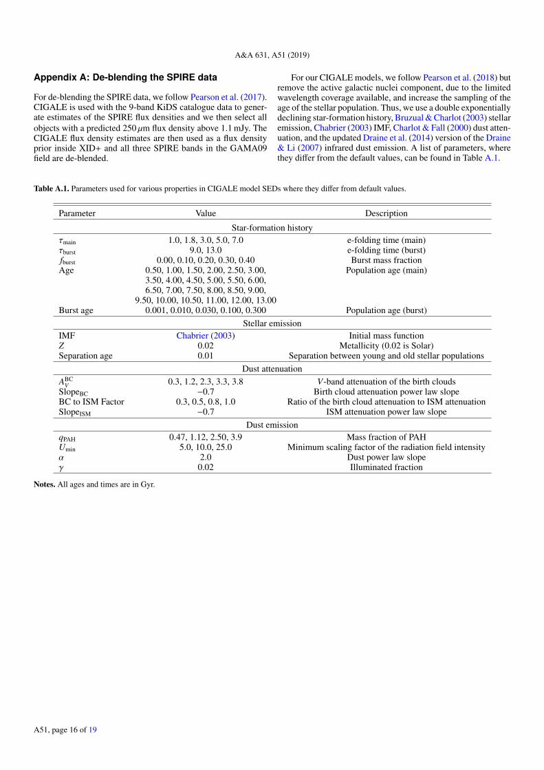
A&A 631, A51 (2019)
Appendix A: De-blending the SPIRE data
For de-blending the SPIRE data, we follow Pearson et al. (2017).CIGALE is used with the 9-band KiDS catalogue data to gener-ate estimates of the SPIRE flux densities and we then select allobjects with a predicted 250 µm flux density above 1.1 mJy. TheCIGALE flux density estimates are then used as a flux densityprior inside XID+ and all three SPIRE bands in the GAMA09field are de-blended.
For our CIGALE models, we follow Pearson et al. (2018) butremove the active galactic nuclei component, due to the limitedwavelength coverage available, and increase the sampling of theage of the stellar population. Thus, we use a double exponentiallydeclining star-formation history, Bruzual & Charlot (2003) stellaremission, Chabrier (2003) IMF, Charlot & Fall (2000) dust atten-uation, and the updated Draine et al. (2014) version of the Draine& Li (2007) infrared dust emission. A list of parameters, wherethey differ from the default values, can be found in Table A.1.
Table A.1. Parameters used for various properties in CIGALE model SEDs where they differ from default values.
Parameter Value Description
Star-formation historyτmain 1.0, 1.8, 3.0, 5.0, 7.0 e-folding time (main)τburst 9.0, 13.0 e-folding time (burst)fburst 0.00, 0.10, 0.20, 0.30, 0.40 Burst mass fractionAge 0.50, 1.00, 1.50, 2.00, 2.50, 3.00, Population age (main)
3.50, 4.00, 4.50, 5.00, 5.50, 6.00,6.50, 7.00, 7.50, 8.00, 8.50, 9.00,
9.50, 10.00, 10.50, 11.00, 12.00, 13.00Burst age 0.001, 0.010, 0.030, 0.100, 0.300 Population age (burst)
Stellar emissionIMF Chabrier (2003) Initial mass functionZ 0.02 Metallicity (0.02 is Solar)Separation age 0.01 Separation between young and old stellar populations
Dust attenuationABC
V 0.3, 1.2, 2.3, 3.3, 3.8 V-band attenuation of the birth cloudsSlopeBC −0.7 Birth cloud attenuation power law slopeBC to ISM Factor 0.3, 0.5, 0.8, 1.0 Ratio of the birth cloud attenuation to ISM attenuationSlopeISM −0.7 ISM attenuation power law slope
Dust emissionqPAH 0.47, 1.12, 2.50, 3.9 Mass fraction of PAHUmin 5.0, 10.0, 25.0 Minimum scaling factor of the radiation field intensityα 2.0 Dust power law slopeγ 0.02 Illuminated fraction
Notes. All ages and times are in Gyr.
A51, page 16 of 19
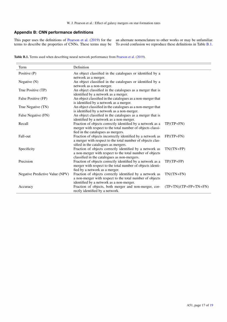
W. J. Pearson et al.: Effect of galaxy mergers on star-formation rates
Appendix B: CNN performance definitions
This paper uses the definitions of Pearson et al. (2019) for theterms to describe the properties of CNNs. These terms may be
an alternate nomenclature to other works or may be unfamiliar.To avoid confusion we reproduce these definitions in Table B.1.
Table B.1. Terms used when describing neural network performance from Pearson et al. (2019).
Term Definition
Positive (P) An object classified in the catalogues or identified by anetwork as a merger.
Negative (N) An object classified in the catalogues or identified by anetwork as a non-merger.
True Positive (TP) An object classified in the catalogues as a merger that isidentified by a network as a merger.
False Positive (FP) An object classified in the catalogues as a non-merger thatis identified by a network as a merger.
True Negative (TN) An object classified in the catalogues as a non-merger thatis identified by a network as a non-merger.
False Negative (FN) An object classified in the catalogues as a merger that isidentified by a network as a non-merger.
Recall Fraction of objects correctly identified by a network as amerger with respect to the total number of objects classi-fied in the catalogues as mergers.
TP/(TP+FN)
Fall-out Fraction of objects incorrectly identified by a network asa merger with respect to the total number of objects clas-sified in the catalogues as mergers.
FP/(TP+FN)
Specificity Fraction of objects correctly identified by a network asa non-merger with respect to the total number of objectsclassified in the catalogues as non-mergers.
TN/(TN+FP)
Precision Fraction of objects correctly identified by a network as amerger with respect to the total number of objects identi-fied by a network as a merger.
TP/(TP+FP)
Negative Predictive Value (NPV) Fraction of objects correctly identified by a network asa non-merger with respect to the total number of objectsidentified by a network as a non-merger.
TN/(TN+FN)
Accuracy Fraction of objects, both merger and non-merger, cor-rectly identified by a network.
(TP+TN)/(TP+FP+TN+FN)
A51, page 17 of 19

A&A 631, A51 (2019)
Appendix C: Example non-mergers and mergers
Here we present example non-mergers and mergers as defined bythe CNN. The images shown are all 64× 64 pixel images with
Fig. C.1. Examples of non-merging galaxies (top row) and merg-ing galaxies (bottom nine rows) for SDSS data set as defined bythe CNN. Images are gri composite with a size of 64× 64 pixel or13.7× 13.7 arcsec.
gri composite for SDSS, Fig. C.1, greyscale r-band for KiDS,Fig. C.2, and 1.6 µm, 1.25 µm, 814 nm composite for CAN-DELS, Fig. C.3.
Fig. C.2. Examples of non-merging galaxies (top row) and merg-ing galaxies (bottom nine rows) for KiDS data set as defined by theCNN. Images are greyscale r-band with a size of 64× 64 pixel or25.3× 25.3 arcsec.
A51, page 18 of 19

W. J. Pearson et al.: Effect of galaxy mergers on star-formation rates
Fig. C.3. Examples of non-merging galaxies (top row) and merginggalaxies (bottom nine rows) for CANDELS data set as defined by theCNN. Images are 1.6 µm, 1.25 µm, 814 nm composite with a size of64× 64 pixel or 3.8× 3.8 arcsec.
A51, page 19 of 19