EFFECT OF EXPERIENCE SAMPLING SCHEDULES ON RESPONSE …
20
1 2 3 4 5 6 7 8 9 10 11 12 13 14 15 16 17 18 19 20 21 22 23 24 25 26 27 28 29 30 31 32 33 34 35 36 37 38 39 40 41 42 43 44 45 46 47 48 49 50 51 52 53 54 55 56 57 58 59 60 61 62 63 64 65 1 EFFECT OF EXPERIENCE SAMPLING SCHEDULES ON RESPONSE RATE AND RECALL ACCURACY OF OBJECTIVE SELF-REPORTS Niels van Berkel, The University of Melbourne Jorge Goncalves, The University of Melbourne Lauri Lovén, University of Oulu Denzil Ferreira, University of Oulu Simo Hosio, University of Oulu Vassilis Kostakos, The University of Melbourne ABSTRACT The Experience Sampling Method is widely used to collect human labelled data in the wild. Using this methodology, study participants repeatedly answer a set of questions, constructing a rich overview of the studied phenomena. One of the methodological decisions faced by researchers is deciding on the question scheduling. The literature defines three distinct schedule types: randomised, interval-based, or event-based (in our case, smartphone unlock). However, little evidence exists regarding the side-effects of these schedules on response rate and recall accuracy, and how they may bias study findings. We evaluate the effect of these three contingency configurations in a 3-week within-subjects study (N=20). Participants answered various objective questions regarding their phone usage, while we simultaneously establish a ground-truth through smartphone instrumentation. We find that scheduling questions on phone unlock yields a higher response rate and accuracy. Our study provides empirical evidence for the effects of notification scheduling on participant responses, and informs researchers who conduct experience sampling studies on smartphones. KEYWORDS Experience Sampling Method; ESM; Ecological Momentary Assessment; EMA; self-report; smartphone; contingency; response rate; accuracy; sampling; mobile questionnaires; data quality; validation. RESEARCH HIGHLIGHTS We investigate the effect of random, interval, and smartphone-unlock based questionnaires Scheduling configuration affects participants’ response rates Recall accuracy of participants is affected by different scheduling configurations The use of combined scheduling techniques should be considered in future ESM studies 1 INTRODUCTION To collect data on human behaviour ‘in the wild’, researchers have adopted the use of in situ data collection methods. One popular method is the Experience Sampling Method (ESM) [38], also known as Ecological Momentary Assessment (EMA). In an ESM study, participants are repeatedly asked a set of questions during their daily lives. Typically, data collection occurs multiple times per day over a period of several days or weeks, allowing for a detailed analysis of the phenomena under investigation [38]. An important mechanism in experience sampling is the adoption of notifications, used to inform participants when a questionnaire should be answered. This stands in contrast with the diary study, in which participants are traditionally not actively informed to provide data. Participants in an ESM study can either comply with these requests for information, dismiss, or ignore it (deliberately or unwittingly). Study notifications – i.e., prompts to answer a questionnaire – can be triggered by a variety of schedule configuration alternatives, categorised into three contingency categories [6, 55]: randomly distributed (signal contingent), following a time interval (interval contingent), or triggered by a specific event (event contingent). In ESM studies, it is crucial that the response rate is high, otherwise the data may be considered unreliable. Similarly, researchers strive to ensure participant input is as accurate as possible to ensure reliability of data analysis and results. Yet, it remains challenging to compare the effect of the three scheduling types on participants’ responses due to the effect of other methodological parameters. For example, participants’ response rate has been said to depend on participants’ attachment to the study results [38], number of notifications [15], communicating response rates to participants [6], effort required to complete a questionnaire [15], and notification expiry time. Surprisingly, few of these have been evaluated systematically, and researchers are limited to using their intuition about their effects when designing studies. Furthermore, the *Manuscript Click here to view linked References
Transcript of EFFECT OF EXPERIENCE SAMPLING SCHEDULES ON RESPONSE …

1 2 3 4 5 6 7 8 9 10 11 12 13 14 15 16 17 18 19 20 21 22 23 24 25 26 27 28 29 30 31 32 33 34 35 36 37 38 39 40 41 42 43 44 45 46 47 48 49 50 51 52 53 54 55 56 57 58 59 60 61 62 63 64 65
1
EFFECT OF EXPERIENCE SAMPLING SCHEDULES ON RESPONSE
RATE AND RECALL ACCURACY OF OBJECTIVE SELF-REPORTS
Niels van Berkel, The University of Melbourne
Jorge Goncalves, The University of Melbourne
Lauri Lovén, University of Oulu
Denzil Ferreira, University of Oulu
Simo Hosio, University of Oulu
Vassilis Kostakos, The University of Melbourne
ABSTRACT
The Experience Sampling Method is widely used to collect human labelled data in the wild. Using this
methodology, study participants repeatedly answer a set of questions, constructing a rich overview of the
studied phenomena. One of the methodological decisions faced by researchers is deciding on the question
scheduling. The literature defines three distinct schedule types: randomised, interval-based, or event-based (in
our case, smartphone unlock). However, little evidence exists regarding the side-effects of these schedules on
response rate and recall accuracy, and how they may bias study findings. We evaluate the effect of these three
contingency configurations in a 3-week within-subjects study (N=20). Participants answered various objective
questions regarding their phone usage, while we simultaneously establish a ground-truth through smartphone
instrumentation. We find that scheduling questions on phone unlock yields a higher response rate and accuracy.
Our study provides empirical evidence for the effects of notification scheduling on participant responses, and
informs researchers who conduct experience sampling studies on smartphones.
KEYWORDS
Experience Sampling Method; ESM; Ecological Momentary Assessment; EMA; self-report; smartphone;
contingency; response rate; accuracy; sampling; mobile questionnaires; data quality; validation.
RESEARCH HIGHLIGHTS We investigate the effect of random, interval, and smartphone-unlock based questionnaires
Scheduling configuration affects participants’ response rates
Recall accuracy of participants is affected by different scheduling configurations
The use of combined scheduling techniques should be considered in future ESM studies
1 INTRODUCTION
To collect data on human behaviour ‘in the wild’, researchers have adopted the use of in situ data collection
methods. One popular method is the Experience Sampling Method (ESM) [38], also known as Ecological
Momentary Assessment (EMA). In an ESM study, participants are repeatedly asked a set of questions during
their daily lives. Typically, data collection occurs multiple times per day over a period of several days or weeks,
allowing for a detailed analysis of the phenomena under investigation [38]. An important mechanism in
experience sampling is the adoption of notifications, used to inform participants when a questionnaire should be
answered. This stands in contrast with the diary study, in which participants are traditionally not actively
informed to provide data. Participants in an ESM study can either comply with these requests for information,
dismiss, or ignore it (deliberately or unwittingly). Study notifications – i.e., prompts to answer a questionnaire –
can be triggered by a variety of schedule configuration alternatives, categorised into three contingency
categories [6, 55]: randomly distributed (signal contingent), following a time interval (interval contingent), or
triggered by a specific event (event contingent).
In ESM studies, it is crucial that the response rate is high, otherwise the data may be considered unreliable.
Similarly, researchers strive to ensure participant input is as accurate as possible to ensure reliability of data
analysis and results. Yet, it remains challenging to compare the effect of the three scheduling types on
participants’ responses due to the effect of other methodological parameters. For example, participants’
response rate has been said to depend on participants’ attachment to the study results [38], number of
notifications [15], communicating response rates to participants [6], effort required to complete a questionnaire
[15], and notification expiry time. Surprisingly, few of these have been evaluated systematically, and
researchers are limited to using their intuition about their effects when designing studies. Furthermore, the
*ManuscriptClick here to view linked References

1 2 3 4 5 6 7 8 9 10 11 12 13 14 15 16 17 18 19 20 21 22 23 24 25 26 27 28 29 30 31 32 33 34 35 36 37 38 39 40 41 42 43 44 45 46 47 48 49 50 51 52 53 54 55 56 57 58 59 60 61 62 63 64 65
2
specific event responsible for triggering notifications in an event contingent-based schedule can be virtually
anything – increasing the complexity of comparing these different contingencies. In this work, we therefore opt
to choose an event which is actively used in HCI studies: unlocking of the participant’s smartphone (see e.g.,
[10, 24, 46]).
In this study, we compare three ESM contingency types to assess whether they affect participants’ response rate
and accuracy. Measurement of ESM response accuracy is notoriously challenging because self-report data often
lacks absolute ground truth data (e.g., someone’s emotional state). Because our study investigates quantifiable
and objective aspects of smartphone usage (e.g., usage duration), we are able to compare participants’ reports of
their personal smartphone usage against ground truth data of their actual usage. Our findings help researchers
overcome the intrinsic challenges of collecting participant data using the ESM on smartphones. While the
choice for a certain notification contingency configuration sometimes follows from the study design and not
vice versa, our results quantify the effects of these methodological decisions on participants’ response rate and
recall accuracy.
2 RELATED WORK
The methods to study human behaviour takes many forms, ranging from lab interviews to ethnographic
fieldwork. A common way of collecting intrinsic data such as human emotions or thoughts, is to intermittently
ask study participants to answer a set of questions during their daily activities. This repetition leads to a more
complete overview of the participants’ daily life if compared to a single one-time questionnaire, as “little
experiences of everyday life fill most of our waking time and occupy the vast majority of our conscious
attention” [55]. For such repeated inquiries, the Experience Sampling Method [38] is a popular choice. Three
key characteristics of the ESM are highlighted in Larson’s seminal publication; “it obtains information about
the private as well as the public parts of people’s lives, it secures data about both behavioural and intrapsychic
aspects of daily activity, and it obtains reports about people’s experience as it occurs, thereby minimizing the
effects of reliance on memory and reconstruction” [38]. Since its introduction, the methodology has been used
to study a wide range of topics (e.g., substance usage [52], educational practices [44], evaluation of ubicomp
technology [27]) and has seen increased uptake in the HCI community [8], indicating the method’s wide
applicability.
2.1 ESM Study Configuration
A core element of the ESM is to notify participants when to complete a certain questionnaire. Albeit the ESM in
its original form only describes the use of randomly triggered notifications, the current consensus is to
distinguish three main ESM notification trigger types [6, 8, 55]:
Signal contingent, in which the timing of notifications is randomised over a predefined duration;
Interval contingent, in which timing of notifications follows a predefined time schedule;
Event contingent, in which specific (measurable) events result in the presentation of a notification.
These events can be related to the usage of the device (e.g., unlocking the device [10]), or following a
change in readings from a device sensor (e.g., the microphone [39]).
Literature highlights various concerns for each of these respective notification trigger types. Signal contingent
notifications are unlikely to capture relatively rare events (e.g., interactions with friends or partners [55]),
therefore requiring a longer study duration to collect a usable quantity of data. Interval contingent notifications
are likely to be distant in time from the event being recorded, introducing retrospection bias [55]. In addition,
the consistent repetition might result in participants being able to predict the occurrence of the next notification,
possibly introducing cognitive bias [15]. Event contingent notifications rely solely on the event that is being
observed, and in the case of an uncommon event only a few notifications will be sent to study participants.
Event contingent notifications can also be prone to design bias as the result of contextual dissonance [39] — the
choice of event triggering the notification directly influences the number of notifications. In addition, the ability
to anticipate incoming alerts may result in behavioural reactivity [25].
In addition to these trigger-specific concerns, the literature also describes two concerns related to the general
experience sampling methodology [5, 51]. By continuously asking participants to focus on one aspect of their
lives, the method may not only measure but also influence the participant’s behaviour. This may have a positive
outcome for the study participant (e.g., by acting as an intervention technique for mental health patients [5]),
however it can also negatively affect the reliability of study results – this phenomenon is called measurement
reactivity. Furthermore, response fatigue describes the notion that both the number and quality of participant
responses decreases over time due to a decreasing interest in contributing to the study. We discuss both these
concerns in more detail below.

1 2 3 4 5 6 7 8 9 10 11 12 13 14 15 16 17 18 19 20 21 22 23 24 25 26 27 28 29 30 31 32 33 34 35 36 37 38 39 40 41 42 43 44 45 46 47 48 49 50 51 52 53 54 55 56 57 58 59 60 61 62 63 64 65
3
2.2 Response Rate
A study’s response rate (i.e., compliance rate) is the ratio of successfully answered questionnaire notifications
over the received notifications. Many factors can potentially influence a participant’s response rate. Typically, a
higher response rate reflects a more accurate observation of the participant’s experience, as a larger portion of
the studied phenomenon is captured. Factors that have been identified to influence participants’ response rate
include: participant attachment [38], study fatigue [53], technical difficulties (e.g., failure in transmission,
crashes) [15], motivational elements (e.g., gamification) [9], as well as study design choices such as notification
expiry time (allowing more time to answer a questionnaire before it expires).
Various studies have investigated ways of increasing response rate in experience sampling studies. Litt et al.
[42] describe the use of “booster” telephone calls, in which participants received phone calls to encourage
compliance. Naughton et al. [45] increase response rate by an average of 16% by sending a follow-up reminder
after 24-hours, with little benefit reported on extending reminders to 48 hours. Kapoor and Horvitz [31] test four
different sampling strategies, ranging in sophistication from randomly timed notifications to the use of a
predictive interruptibility model. Employed on a desktop computer, the system identifies usage behaviour (e.g.,
typing) as well as external signals (e.g., calendar events). Interestingly, the different probing mechanisms led to
a high difference in average number of notifications (4.65 notifications for ‘decision-theoretic dynamic
probing’, 21.35 notifications for random probing). In 73.08% of random notifications, participants indicated
they were too busy to respond to the probe, whereas participants in the decision-theoretic dynamic probing
condition indicated to be too busy in 46.63% of cases. Although participants indicated to be less busy in this
model, the high difference in notifications highlights a potential pitfall of a dynamic notification scheme. Lathia
et al. [39] compare the effect of four different sensor-based notification triggers (following a ‘social event’ (text
message or phone call), change in location, microphone detecting silence, and microphone detecting noise).
Their results show that these event-based sampling techniques do not collect responses distributed evenly over
the course of day, introducing bias into the data collection. In addition, there are significant differences in the
level of self-reported affect between these sensor-based schedules. While not further dissecting these
differences, the authors note that “our design parameters influence the outcome, and any inferences made on
such data should take into account that design will influence the view that researchers will build of their
participants” [39]. Our study builds upon this work by collecting self-reports for which ground-truth data is
available, allowing for the measurement of participant accuracy.
Response Fatigue
The gradual decline of response rate over the duration of the study is a well-documented phenomenon (e.g., [45,
53]). Hsieh et al. [26] were one of the first to study this behaviour, and improved participant compliance over
time by providing visual feedback to the participant through a comparative study (visual feedback vs no
feedback).
Fuller-Tyszkiewicz et al. [23] investigate response fatigue and find that “demands of ESM protocol undermine
quantity more so than quality of obtained data” [23]. Although the sample size of the study was considerable (N
= 105), the study duration was limited to 7 days – with many ESM studies being of longer duration. Reynolds et
al. [48] report on a study on parent-child relationships, using the methodologically related diary method over a
period of 56 days. Participants were requested to complete one diary entry per day (as opposed to multiple daily
entries in an ESM study). As the study progressed, participants completed less diary entries on weekdays, with
no change on weekends. As child and parent separately reported on the same events, the authors analysed the
change in agreement over time and found that the agreement between parent and child slightly declined as the
study progressed. As such, response fatigue did not only affect response rate, but also the quality of the
participant response [48].
2.3 Participant Response Accuracy
The ESM is specifically designed to increase participant response accuracy by reducing reliance on participants’
long term memory to reconstruct past events [38]. Participant reflection on past events through long term
memory has been shown to be unreliable, reducing the validity of collected research data [28]. However, the
accuracy of ESM responses itself remains understudied [7], despite being referred to as the gold standard in
measurement of affective experience of daily life and is used as a benchmark against other methods [37]. As
affective experience is inherently personal, establishing a baseline to measure accuracy is challenging. In their
analysis of reliability and validity of experience sampling for children with autism spectrum disorders, Chen et
al. [13] ran a 7-day long study in which participants answered questions concerning their activity, experience,
and emotion. Through a split-week analysis (comparing data from the start of the week to data from the end of

1 2 3 4 5 6 7 8 9 10 11 12 13 14 15 16 17 18 19 20 21 22 23 24 25 26 27 28 29 30 31 32 33 34 35 36 37 38 39 40 41 42 43 44 45 46 47 48 49 50 51 52 53 54 55 56 57 58 59 60 61 62 63 64 65
4
the week), the authors find no significant difference between quality of experiences and associated emotions,
suggesting a high internal reliability.
3 EXPERIMENTAL DESIGN
We designed an experiment where participants use their smartphones to answer a set of questions regarding
their perceived smartphone usage. In addition, we collected ground truth data by logging actual smartphone
usage in the background. ESM notifications were presented according to one of the following experimental
conditions:
Condition A - Signal contingent (random). The presentation of notifications is randomised (using a
uniform randomisation scheme) over the duration of the day. We enforce a set limit of six notifications
per day, without regards for the fact whether the notification is unanswered. The time-window within
which the timing of the notifications is randomised ranges between 10:00 to 20:00 to avoid night-time
alerts.
Condition B - Interval contingent (bi-hourly). Notifications are scheduled to occur every two hours
between 10:00 and 20:00 (i.e., at 10:00, 12:00, […], 20:00). This results in a total of six notifications
presented to our participants over the course of the day.
Condition C – Smartphone unlock (i.e., following an unlock event). Notifications are presented
when the participant unlocks the mobile phone, considering pre-configured time sets. Identical to
Conditions A and B, we send a maximum of six notifications per day. A time constraint is added to
ensure notifications are spread over the duration of the day, consisting of 6 time-bins of equal duration
(e.g., 10:00 to 11:40, 11:40 to 13:20, […], 18:20 to 20:00). In case the phone has already been
unlocked in the current time-bin, no new notification is shown — regardless of whether the notification
was answered. If the phone of the participant is not unlocked in a given time-bin, no notification is
shown. We chose the unlock event in our notification configuration because this event is widely used
in the literature (e.g., [10, 21, 24, 56]) and acts as a precedent to many other smartphone interactions.
As such, the design of our study does not aim to encompass all notification events or generalise to all
possible event contingent configurations.
All conditions have a maximum of six notifications per day. We applied a notification expiry time of 15 minutes
after which the notifications were dismissed and no longer shown to the participant. In addition, we logged
whether notifications expired or actively dismissed by the participant. Finally, participants were not able to
initiate data submissions themselves.
3.1 Study Parameters
We use a balanced Latin Square to distribute our participants over the three conditions, reducing the risk of
order effects (e.g., fatigue, loss of interest, learning) on our data. As we have an odd number of conditions in our
study, we apply a double Latin Squares design (i.e., second square is a mirror of the first) in the distribution of
our participants. For example, some participants begun our study in Condition C for a week, then switched to B
for a week, and finally to A for another week. We balanced participants equally over each ‘square’ in the double
Latin Square design. Our 21-day long deployment is in line with recommendations from Stone et al. [53] —
data quality deteriorates after a period of 2-4 weeks. Each condition is applied for seven full days before a new
condition is introduced, resembling an authentic study configuration as opposed to randomly distributing the
conditions over the entire duration of this study.
3.2 ESM Questionnaire
All the ESM questions are identical in all conditions. The questionnaire consists of three questions regarding
recent smartphone usage, one question on the level of interruption of the notification, and one self-assessment of
the response accuracy. The questions on smartphone usage include the number of unique applications used
(shown to be context dependent [16], thus changing throughout the day), duration of smartphone usage (both
diverse across users [18] and challenging for users to estimate accurately [2]), and number of times the phone
was turned on (challenging for users to accurately estimate [2]). We explicitly instructed participants to include
the number of locked screen-glances (e.g., checking notifications, time) in their answers. We base our questions
regarding the level of interruption of notification timing on [21].
We phrase our question to specifically mention the amount of time since the last notification was presented,
regardless of the fact whether this notification was answered by the participant. This also makes it clear for the
participant as to what exactly is being asked. For example: “How many unique applications have you used since
12:00?”. For the first notification of each day, we ask participants to answer the question for the timespan
following 08:00 up to the current time. The question set consists of five questions in total. As aforementioned,

1 2 3 4 5 6 7 8 9 10 11 12 13 14 15 16 17 18 19 20 21 22 23 24 25 26 27 28 29 30 31 32 33 34 35 36 37 38 39 40 41 42 43 44 45 46 47 48 49 50 51 52 53 54 55 56 57 58 59 60 61 62 63 64 65
5
three of those questions target smartphone usage (number of unique applications, duration of phone usage in
minutes, and number of times the screen of the phone was turned on), presenting the participant with a numeric
input field. The final two questions focus on the questionnaire itself (“How confident are you in your answers?”
and “Was this an appropriate time to interrupt you with these questions?”). These last two questions present the
participant with a 5-point Likert-scale ranging from [not at all confident / very inappropriate] to [very confident
/ very appropriate].
Finally, participants completed an exit questionnaire online after the study ended to collect information on
general smartphone usage, notification-interaction habits, and the participants’ perception in answering the ESM
questions.
3.3 Data Collection
Data was collected using a custom-made application that was installed through the Google Play Store (private
beta release). The application was running continuously in the background of the participants’ personal device.
Using this application, based on the AWARE mobile instrumentation framework [20], we collect not only the
participants’ responses but also log, inter alia, the following data: phone usage, application usage, ESM answer,
and ESM question status (i.e., expired, answered, dismissed). The application is also responsible for sending
notifications to participants. Notifications appeared as regular notifications on the participants phone, with the
questionnaire opening when the notification is touched.
4 METHOD
4.1 Recruitment
A total of 24 participants participated in this study. We omit contributions from 4 participants who encountered
miscellaneous device incompatibility issues leading to partial data loss, leaving 20 participants in total (average
age 26.4 (± 4.6) years old, 5 women, 15 men). As a result, our Latin Square design (Section 3.1) is no longer
complete. We report the final distribution of participants over conditions in Table 1 below. Participants were
recruited from our university campus using mailing lists and had a diverse educational background. To
minimise the novelty effect and ensure proper device operation, participants used their personal device.
A - Signal B - Interval C - Unlock
Week 1 6 7 7
Week 2 7 8 5
Week 3 7 5 8
Table 1. Final distribution of participants across conditions over study period.
4.2 Procedure
We invited all participants for an individual training session in our lab. During this session, we explained our
interest in the way they use their smartphone in daily life. We did not inform them of the different contingency
types that would be evaluated. To set expectations on the level of participant strain, we explained that we would
send a maximum of six notifications per day between 10:00 and 20:00. In addition, we explained each of the
five ESM questions one-by-one to ensure participants understood the questions we asked them to answer.
Following the explanation of the ESM questions, we informed participants about the data logging capabilities of
our application and installed the necessary software on the participant’s phone. We explained to our participants
how we interpret ‘smartphone usage’ for the purpose of this study: any moment at which the smartphone screen
is turned on. Participants were given practical examples to ensure their reports are in line with our expectations
(e.g., listening to music with the screen turned off is not considered as usage). Due to technical limitations of
Android OS, we are unable to distinguish between ‘real’ smartphone usage and the user putting away their
phone after usage without turning off the screen (i.e., resulting in a timeout). We explicitly instructed
participants to include the number of locked screen-glances (e.g., checking notifications, time) in their answers.
All deployments lasted for 21 days, and were followed by an exit questionnaire. Participants received two movie
vouchers as compensation.
4.3 Data Analysis

1 2 3 4 5 6 7 8 9 10 11 12 13 14 15 16 17 18 19 20 21 22 23 24 25 26 27 28 29 30 31 32 33 34 35 36 37 38 39 40 41 42 43 44 45 46 47 48 49 50 51 52 53 54 55 56 57 58 59 60 61 62 63 64 65
6
We aim to provide Bayesian statistics as currently discussed in the broader HCI community. This brings
forward a focus on effect size and uncertainty in an attempt to “convey uncertainty more faithfully” [33] and
provide a more useful presentation of our results for both academics and practitioners. To this end, we use
Bayes factors over p-values for hypothesis testing and credible intervals (using highest posterior density) over
confidence intervals. The use of p-values has faced increased scrutiny (e.g., [32, 54]), mainly due to the
incorrect interpretation and application by researchers.
Bayes factors provide an intuitive way of comparing hypotheses by quantifying the likelihood of competing
hypotheses as a ratio. This enables a direct comparison between models. For example, a Bayes factor of 15
indicates that the collected data is 15 times more probable if H1 were true than if the null hypothesis H0 were
true. In formula form this becomes:
, with D denoting data observed in the study. Throughout
our analysis we use the BayesFactor package [43] for R. Given our within-subjects design, our analysis consists
mainly of ‘Bayesian ANOVA’, as described in [50]. The BayesFactor provides default priors for common
research designs. In our models, we consistently treat participants as a random factor as per the study’s design.
Using posterior estimation, we compare the study conditions through credible intervals. Credible intervals are
calculated using the 95% Highest Posterior Density interval (HPD) through the bayesboot package [3]. We
adopt the interpretation of Bayes factors’ significance as put forward by Jeffreys [29] and refined by Lee and
Wagenmakers [40].
5 RESULTS
A theoretical maximum of 2520 notifications (840 per condition) could be sent during the study (6 notifications
per day, 20 participants, 21 days). A total number of 2313 notifications were issued during the study. This
difference is due to the phone running out of power, the phone being turned off, or the participant not using the
device during a given timeslot (Condition C) – occurrences which are beyond our control. Our results highlight
a considerable effect of condition on response rate, two out of three accuracy measures, and self-reported
confidence levels. Study condition did not affect perceived level of interruption. We discuss the detailed results
of each dependent variable below.
5.1 Response Rate
A total of 2313 ESM notifications were triggered over the duration of the study, with each notification
consisting of 5 questions. The average response rate over all conditions was 59.7%. Many unanswered ESM
questionnaires were the result of notification expiration (39.3% of total), with only 1.0% being actively
dismissed by a participant. We sent a total of 814 randomly timed notifications in Condition A, and 806
scheduled notifications were sent for Condition B. For Condition C, a total of 693 notifications were sent upon
phone unlock (out of a total of 4190 unlock events between 10:00 and 20:00 for days on which Condition C was
active, 16.5%). Table 2 presents an overview of response rate results as split per condition.
A - Signal B - Interval C - Unlock
Notifications sent 814 806 693
Response rate 51.6% 51.6% 76.8%
Notifications answered 420 416 532
95% HPD [47.14, 56.89] [47.18, 56.73] [72.70, 81.83]
Expired 46.5% 47.8% 22.1%
Dismissed 1.9% 0.6% 1.1%
Table 2. Notification behaviour and response rate.
We compute the effect of condition on response rate. A JZS Bayes factor within-subjects ANOVA with default
prior (non-informative Jeffreys prior) revealed a Bayes factor of 1.37 x 10²⁰
, providing extreme evidence for the
existence of an effect of condition on response rate. We calculate a 95% HPD per condition and report these in
Figure 1 and Table 2.

1 2 3 4 5 6 7 8 9 10 11 12 13 14 15 16 17 18 19 20 21 22 23 24 25 26 27 28 29 30 31 32 33 34 35 36 37 38 39 40 41 42 43 44 45 46 47 48 49 50 51 52 53 54 55 56 57 58 59 60 61 62 63 64 65
7
Figure 1. Posterior distribution of response rate.
Figure 1 shows the overall effect of the three conditions on the participants’ response rate. As can been seen
from Figure 2, Condition C results in the highest response rate for 17 out of 20 participants. This shows that the
effect is consistent across participants, even for those that have an overall lower tendency to respond to ESMs.
Figure 2. Average response rate per participant and condition means (Condition A and B overlap).
Effect of Day and Time on Response Rate
Our study lasted 21 days, with the ESM response rate remaining fairly constant throughout the study. In Figure
3, a ‘wave’ effect is visible, indicating minor variance among participant clusters (study condition changed
every 7 days). We compute the effect of relative study day on response rate, regardless of study condition. A
JZS Bayes factor within-subjects ANOVA with default prior revealed a Bayes factor of 0.08, providing
moderate evidence for the lack of effect of study day on response rate. The response rate changes over time of
day, as visible in Figure 3. Condition B display a sharp drop in response rate in the morning hours when
compared to the other conditions.
Figure 3. Response rate over study day and time of day.
Recall Accuracy
We measure the recall accuracy of participants by comparing participants’ answers against the actual data as
logged passively on participants’ phones. For the three questions focused on recall accuracy, we calculate both
the mean average error (MAE) and the root-mean-square error (RMSE). MAE and RMSE are traditionally used
to measure accuracy of a model’s prediction. Lower scores indicate higher accuracy.
50%
60%
70%
80%
Condition A Condition B Condition C
Re
sp
on
se
ra
te
0%
25%
50%
75%
100%
P0
1
P0
2
P0
3
P0
4
P0
5
P0
6
P0
7
P0
9
P1
0
P1
1
P1
2
P1
3
P1
4
P1
6
P1
8
P1
9
P2
0
P2
1
P2
2
P2
4
Re
sp
on
se
ra
te
Condition A Condition B Condition C
0%
25%
50%
75%
100%
1 5 10 15 20
Relative study day
Re
sp
on
se
ra
te
0%
25%
50%
75%
100%
10:00 12:00 14:00 16:00 18:00 20:00
Time of day
Re
sp
on
se
ra
te
Condition A Condition B Condition C

1 2 3 4 5 6 7 8 9 10 11 12 13 14 15 16 17 18 19 20 21 22 23 24 25 26 27 28 29 30 31 32 33 34 35 36 37 38 39 40 41 42 43 44 45 46 47 48 49 50 51 52 53 54 55 56 57 58 59 60 61 62 63 64 65
8
Usage Duration
We asked participants to report the duration of their smartphone usages in minutes. We calculate the sum
duration of phone usage activities for the time period as asked by each specific question. This is measured by
calculating the time difference between the screen of the device being unlocked and the screen of the device
being turned off. See Table 3 for an overview of these results.
A - Signal B - Interval C - Unlock
Observed mean (SD) 24.55
(± 28.47)
27.36
(± 29.05)
17.10
(± 24.97)
Self-reported mean (SD) 15.32 (± 16.38) 17.34 (± 16.93) 10.17 (± 18.45)
Mean error ratio 0.32 (± 1.04) 0.33 (± 0.96) 0.37 (± 1.15)
95% HPD [0.21, 0.42] [0.24, 0.43] [0.27, 0.47]
MAE 14.99 16.66 12.81
RMSE 24.98 26.56 25.31
Table 3. Observed and reported screen usage duration (in minutes), including MAE and RMSE.
For each answer provided by the participant we calculate the accompanying error ratio and apply a logarithmic
function to normalise the data from the scale [0, Inf] to the scale [-Inf, Inf]. We then compute the effect of
condition on this calculated error ratio. A JZS Bayes factor for a within-subjects ANOVA model with default
prior revealed a Bayes factor of 0.02, providing very strong evidence for no effect of condition on the
participants’ error. The posterior distribution is shown in Figure 4, and highlights the overlap between
conditions. We calculate the 95% HPD per condition and report these numbers in Table 3. Running the same
test for effect of relative study day on the error value shows a Bayes factor of 0.01, providing very strong
evidence that the participants’ answers were not affected by the longevity of the study.
Figure 4. Posterior distribution of error ratio for self-reported usage duration.
Figure 5 shows a scatterplot of self-reports on screen usage against the recorded observations (in minutes). To
visualise the distribution of these two variables, we add marginal histograms to both axes. The value of self-
reported observations is strongly clustered near ‘round’ numbers (e.g., 5 min., 10 min., etc.), with a high number
of usage durations reported in between the 0 and 5-minute mark. We find evidence that participants
underestimate their smartphone usage duration.
0.2
0.3
0.4
0.5
Condition A Condition B Condition C
Err
or
rati
o o
fu
sag
e d
ura
tio
n

1 2 3 4 5 6 7 8 9 10 11 12 13 14 15 16 17 18 19 20 21 22 23 24 25 26 27 28 29 30 31 32 33 34 35 36 37 38 39 40 41 42 43 44 45 46 47 48 49 50 51 52 53 54 55 56 57 58 59 60 61 62 63 64 65
9
Figure 5. Recorded vs self-reported screen usage duration (in minutes).
Number of Unique Applications
Similar to the calculation of smartphone usage duration, we calculate the number of unique applications used by
our participants in the specified time window. We first eliminate system applications (e.g., launchers,
lockscreens) from out data as recommended in literature [30]. Then we compare the observed number of unique
application with the participant reports and calculate the corresponding MAE and RMSE per condition (Table
4).
A - Signal B - Interval C - Unlock
Observed mean (SD) 5.17 (± 3.30) 5.43 (± 2.88) 3.51 (± 2.58)
Self-reported mean (SD) 3.29 (± 2.95) 3.40 (± 2.57) 2.45 (± 1.72)
Mean error ratio 0.37 (± 0.55) 0.39 (± 0.48) 0.24 (± 0.55)
95% HPD [0.31, 0.43] [0.34, 0.44] [0.18, 0.30]
MAE 2.67 2.58 1.80
RMSE 4.06 3.63 2.65
Table 4. Observed and reported unique applications used, including MAE and RMSE.
Figure 6. Posterior distribution of error ratio for self-reported number of unique apps.
Spearman's ρ = 0.507
0
20
40
60
0 25 50 75 100
Recorded screen usage
Self
-rep
ort
0.2
0.3
0.4
0.5
Condition A Condition B Condition C
Err
or
rati
o o
fu
niq
ue
ap
plic
ati
on
s
1 2 3 4 5 6 7 8 9 10 11 12 13 14 15 16 17 18 19 20 21 22 23 24 25 26 27 28 29 30 31 32 33 34 35 36 37 38 39 40 41 42 43 44 45 46 47 48 49 50 51 52 53 54 55 56 57 58 59 60 61 62 63 64 65
10
Figure 7. Recorded vs self-reported number of apps.
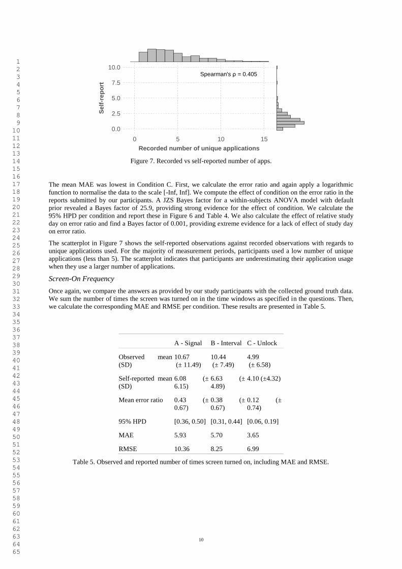
The mean MAE was lowest in Condition C. First, we calculate the error ratio and again apply a logarithmic
function to normalise the data to the scale [-Inf, Inf]. We compute the effect of condition on the error ratio in the
reports submitted by our participants. A JZS Bayes factor for a within-subjects ANOVA model with default
prior revealed a Bayes factor of 25.9, providing strong evidence for the effect of condition. We calculate the
95% HPD per condition and report these in Figure 6 and Table 4. We also calculate the effect of relative study
day on error ratio and find a Bayes factor of 0.001, providing extreme evidence for a lack of effect of study day
on error ratio.
The scatterplot in Figure 7 shows the self-reported observations against recorded observations with regards to
unique applications used. For the majority of measurement periods, participants used a low number of unique
applications (less than 5). The scatterplot indicates that participants are underestimating their application usage
when they use a larger number of applications.
Screen-On Frequency
Once again, we compare the answers as provided by our study participants with the collected ground truth data.
We sum the number of times the screen was turned on in the time windows as specified in the questions. Then,
we calculate the corresponding MAE and RMSE per condition. These results are presented in Table 5.
A - Signal B - Interval C - Unlock
Observed mean
(SD)
10.67
(± 11.49)
10.44
(± 7.49)
4.99
(± 6.58)
Self-reported mean
(SD)
6.08 (±
6.15)
6.63 (±
4.89)
4.10 (±4.32)
Mean error ratio 0.43 (±
0.67)
0.38 (±
0.67)
0.12 (±
0.74)
95% HPD [0.36, 0.50] [0.31, 0.44] [0.06, 0.19]
MAE 5.93 5.70 3.65
RMSE 10.36 8.25 6.99
Table 5. Observed and reported number of times screen turned on, including MAE and RMSE.
Spearman's ρ = 0.405
0.0
2.5
5.0
7.5
10.0
0 5 10 15
Recorded number of unique applications
Self
-re
po
rt

1 2 3 4 5 6 7 8 9 10 11 12 13 14 15 16 17 18 19 20 21 22 23 24 25 26 27 28 29 30 31 32 33 34 35 36 37 38 39 40 41 42 43 44 45 46 47 48 49 50 51 52 53 54 55 56 57 58 59 60 61 62 63 64 65
11
Figure 8. Posterior distribution of error ratio for self-reported times screen on.
The mean MAE was lowest in Condition C. We calculate the error ratio and apply a logarithmic function to
normalise the data, and the compute the effect of condition on the error ratio. A JZS Bayes factor within-
subjects ANOVA with default prior revealed a Bayes factor of 6.34 x 10⁹, providing extreme evidence for an
effect of condition on participant error. We calculate the 95% HPD per condition and report these numbers in
Figure 8 and Table 5. Additionally, a within-subjects ANOVA indicated extreme evidence for the lack of effect
of study day on error rate (Bayes factor = 0.004).
Figure 9. Recorded vs self-reported screen on frequency.
The scatterplot in Figure 9 shows the frequency of screen turn on events, as collected from participant self-
reports and collected ground truth. We see that especially for higher frequencies in screen on events, participants
underestimate these events. The histogram of self-reported observations shows a less visible version of the trend
shown in Figure 5, where self-reports are clustered around ‘round’ numbers.
Confidence
Each ESM questionnaire asked participants to rate their confidence in the accuracy of their answers. Mean
confidence scores are 3.28 (± 0.97), 3.20 (± 1.01), and 3.54 (± 0.99) for Conditions A, B, and C respectively.
We compute the effect of condition on the reported confidence. A JZS Bayes factor within-subjects ANOVA
with default prior revealed a Bayes factor of 5.10 x 10⁵, providing extreme evidence for an effect of condition
on reported confidence. We calculate the 95% HPD per condition: [3.19, 3.38], [3.10, 3.29], and [3.46, 3.62] for
Conditions A, B, and C respectively. Figure 10 shows the distribution of the posterior. In addition, we compute
the effect of relative study day on participant’s confidence level. This results in a Bayes factor of < 0.001,
providing extreme evidence for the lack of an effect of study day on reported confidence.
0.0
0.2
0.4
0.6
Condition A Condition B Condition C
Err
or
rati
o o
fsc
ree
n o
n f
req
ue
ncy
Spearman's ρ = 0.473
0
10
20
30
0 10 20 30 40
Recorded number of screen on frequency
Self
-rep
ort

1 2 3 4 5 6 7 8 9 10 11 12 13 14 15 16 17 18 19 20 21 22 23 24 25 26 27 28 29 30 31 32 33 34 35 36 37 38 39 40 41 42 43 44 45 46 47 48 49 50 51 52 53 54 55 56 57 58 59 60 61 62 63 64 65
12
Figure 10. Posterior distribution for self-reported confidence levels.
Level of Interruption
Final question of each questionnaire asked participants to rate the level of interruption. Mean scores for each
condition are 3.78 (± 1.20), 3.81 (± 1.24), and 3.78 (± 1.27) for Condition A, B, and C respectively. We
compute the effect of condition on the perceived level of interruption for each questionnaire. A JZS Bayes factor
within-subjects ANOVA with default prior revealed a Bayes factor of 0.11, providing moderate evidence for a
lack of effect of condition on perceived interruption. We calculate the 95% HPD per condition: [3.67, 3.90],
[3.69, 3.92], and [3.67, 3.89] for Conditions A, B, and C respectively (see Figure 11). We also compute the
effect of relative study day on the perceived level of interruption, and find a Bayes factor of 0.005, providing
extreme evidence for the lack of an effect of study day on perceived interruption.
Figure 11. Posterior distribution for self-reported level of interruption.
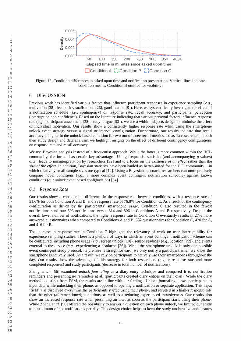
Notification Trigger
The time of notification trigger has a direct effect on the elapsed time since ‘asked upon time’ (time as displayed
in the questions; e.g., ‘[...] used since [xx.xx]?’). Elapsed time thus indicates the timespan for which participants
must answer a question. The notification trigger is randomised in Condition A, thus resulting in a wide range of
elapsed time durations. Condition B presents a notification every 2 hours, providing a constant elapsed time of
120 minutes. In Condition C, notifications are triggered depending on when participants use their phone.
Condition C is therefore the only condition in which notification presentation is not controlled by a system
designed schedule.
We visualise the effect of condition on this elapsed time using a density plot (Figure 12). Condition B is omitted
from the plot as it is centred at the 120-minute mark, and including it reduces the readability of the graph.
Condition A has an average elapsed time of 113 minutes, Condition B an average of 122 minutes, and Condition
C results in the shortest elapsed time of 87 minutes. The density of Condition C shows a strong tendency for a
shorter elapsed time when compared with Condition A. This difference can be accounted for by the frequent
(but brief duration) of smartphone usage, as has been reported in the literature [11, 19]. By multiplying the
average elapsed time with the number of daily notifications and the condition’s respective response rate, we find
the average daily time covered by the answered ESM questions; 349.85 minutes for Condition A, 377.71
minutes for Condition B, and 400.90 minutes for Condition C.
3.0
3.2
3.4
3.6
Condition A Condition B Condition C
Co
nfi
de
nce
lev
el
3.6
3.7
3.8
3.9
4.0
Condition A Condition B Condition C
Lev
el
of
inte
rru
pti
on
1 2 3 4 5 6 7 8 9 10 11 12 13 14 15 16 17 18 19 20 21 22 23 24 25 26 27 28 29 30 31 32 33 34 35 36 37 38 39 40 41 42 43 44 45 46 47 48 49 50 51 52 53 54 55 56 57 58 59 60 61 62 63 64 65
13
Figure 12. Condition differences in asked upon time and notification presentation. Vertical lines indicate
condition means. Condition B omitted for visibility.
6 DISCUSSION
Previous work has identified various factors that influence participant responses in experience sampling (e.g.,
motivation [38], feedback visualisations [26], gamification [9]). Here, we systematically investigate the effect of
a notification schedule (i.e., contingency) on response rate, recall accuracy, and participants’ perception
(interruption and confidence). Based on the literature indicating that various personal factors influence response
rate (e.g., participant attachment [38], study fatigue [53]), we use a within-subjects design to minimise the effect
of individual motivation. Our results show a consistently higher response rate when using the smartphone
unlock event strategy versus a signal or interval configuration. Furthermore, our results indicate that recall
accuracy is higher in the unlock-based condition for two out of three recall metrics. To assist researchers in both
their study design and data analysis, we highlight insights on the effect of different contingency configurations
on response rate and recall accuracy.
We use Bayesian analysis instead of a frequentist approach. While the latter is more common within the HCI-
community, the former has certain key advantages. Using frequentist statistics (and accompanying p-values)
often leads to misinterpretation by researchers [32] and to a focus on the existence of an effect rather than the
size of the effect. In addition, Bayesian statistics have been hauled as better-suited for the HCI community – in
which relatively small sample sizes are typical [12]. Using a Bayesian approach, researchers can more precisely
compare novel conditions (e.g., a more complex event contingent notification schedule) against known
conditions (our unlock event based configuration) [34].
6.1 Response Rate
Our results show a considerable difference in the response rate between conditions, with a response rate of
51.6% for both Condition A and B, and a response rate of 76.8% for Condition C. As a result of the contingency
configuration as driven by the participants’ smartphone usage, Condition C also resulted in the fewest
notifications send out: 693 notifications versus 814 and 806 in Conditions A and B respectively. Despite the
overall lower number of notifications, the higher response rate in Condition C eventually results in 27% more
answered questionnaires when compared to Conditions A and B: 532 questionnaires for Condition C, 420 for A,
and 416 for B.
The increase in response rate in Condition C highlights the relevancy of work on user interruptibility for
experience sampling studies. There is a plethora of ways in which an event contingent notification scheme can
be configured, including phone usage (e.g., screen unlock [10]), sensor readings (e.g., location [22]), and events
external to the device (e.g., experiencing a headache [36]). While the smartphone unlock is only one possible
event contingent study protocol, its premise is straightforward; we only notify a participant when we know the
smartphone is actively used. As a result, we rely on participants to actively use their smartphones throughout the
day. Our results show the advantage of this strategy for both researchers (higher response rate and more
completed responses) and study participants (decrease in total number of notifications).
Zhang et al. [56] examined unlock journaling as a diary entry technique and compared it to notification
reminders and presenting no reminders at all (participants created diary entries on their own). While the diary
method is distinct from ESM, the results are in line with our findings. Unlock journaling allows participants to
input data while unlocking their phone, as opposed to opening a notification or separate application. This input
‘field’ was displayed every time the participants started using their phone, and resulted in a higher response rate
than the other (aforementioned) conditions, as well as a reducing experienced intrusiveness. Our results also
show an increased response rate when presenting an alert as soon as the participant starts using their phone.
While Zhang et al. [56] offered the possibility to answer a question on each phone unlock, we limited our study
to a maximum of six notifications per day. This design choice helps to keep the study unobtrusive and ensures
0.000
0.002
0.004
0.006
50 100 150 200 250 300 350 400+
Elapsed time in minutes since asked upon timeD
en
sit
y
Condition A Condition B Condition C

1 2 3 4 5 6 7 8 9 10 11 12 13 14 15 16 17 18 19 20 21 22 23 24 25 26 27 28 29 30 31 32 33 34 35 36 37 38 39 40 41 42 43 44 45 46 47 48 49 50 51 52 53 54 55 56 57 58 59 60 61 62 63 64 65
14
that the topic at hands is not continuously brought to the attention of the participant – a potential source of
measurement reactivity [5, 48].
Participant response rate, although not always reported by researchers [8], can differ considerably between
participants. This is problematic, as the general interpretation of collected ESM answers will be skewed towards
those participants that did actively contribute. As a result, researchers are sometimes forced to remove from the
analysis participants with a low number of contributions (e.g., [17]). Figure 2 shows the response rate per
participant in our study, including the mean response rate over all participants per condition. Just like in related
work, the response rates in our study differ considerably between participants. However, Figure 2 shows that for
17/20 participants, Condition C outperforms both Conditions A and B. This shows that Condition C’s
notification configuration works across a wide range of participants, including both active contributors as well
as those with an overall lower response rate.
Context is an important aspect to consider when conducting ESM studies. As the context of a participant
regularly changes throughout the day, it is common practice for ESM questionnaires to disappear after a given
amount of time – better known as notification expiry time [8]. In this study, a 15-minute expiry time was used.
Given that notifications were therefore disappearing in 15 minutes, it is likely that participants in Condition A
and B have simply missed some of these notifications altogether (rather than actively ignoring them) –
contributing to the lower response rates in these conditions. However, keeping these notifications alive for
longer durations of time goes against the in-situ nature of Experience Sampling. This approach therefore aligns
with current practice of researchers utilising the ESM.
Summarised, a study’s contingency configuration can significantly affect response rates. In our study, delivering
notification when participants unlocked their smartphones achieved the highest response rates. This contingency
resulted in fewer sent notifications (compared to the other conditions), and a higher number of answered
notifications. Remarks from study participants highlight how a participant’s typical smartphone behaviour may
affect response rates, and why many ESM notifications typically go unanswered; “I usually don't notice
notifications when I am away from home/work, because I used to keep my phone in the bag and check it only
when I need it.” (P12), and “I keep my phone in silence all the time, to not get distracted by the notifications too
often.” (P19). A participant with Condition C scheduled for the last week remarks; “By the end, the notifications
were appearing right when I was free and could easily answer the question.” (P02). Based on these participant
comments, presentation of notifications following phone unlock has a positive effect on both availability and
visibility (i.e., participants are aware that a notification was received and are available and willing to answer it).
We assume that in Condition C, participants noticed all notifications (visibility of 100%), and that those
questionnaires that went unanswered are primarily the result of being interrupted in an ongoing activity (76.8%
availability). For Conditions A and B, which feature almost identical response rates, almost half of the
notifications either went by unnoticed or arrived at a time at which the participant was unable or unwilling to
answer.
Day and Time
Studies employing ESM typically run for a relatively short amount of time, following the observation that data
quality decreases after a period of two to four weeks [53]. As shown in Figure 3, a small reduction in overall
response rate (across study conditions) is visible across the total duration of the study. Dividing the study in 1-
week bins shows a response rate of 62.3%, 58.3%, and 56.6% for study week 1, 2, and 3 respectively. Figure 3
shows participants’ response rate over the duration of the day. Condition B, in which questionnaires are
presented every other hour (10:00, 12:00, [...]), shows a very low response rate in the morning, which increases
in the afternoon (even surpassing Condition C), before dropping slightly in the evening. Poppinga et al. [47]
investigate receptivity of smartphone notifications, and their results also indicate a low response rate in morning
hours, surpassed only by a lower response rate during the night. However, this does not explain the stark
difference between conditions for these hours. Condition B is the only condition in which participants could
precisely anticipate notifications, potentially causing a lower response rate as participants did not want to be
interrupted at the start of their day by an (expected) ESM questionnaire.
The exit questionnaire answers also highlight a difference between participants. Several participants commented
that their willingness to answer diminished during the study – “First week was ok, later my willingness to
answer was decreasing fast. I was happy when it ended.” (P12) and “Last couple of days I had to motivate
myself by remembering the goal and that it's about a real study.” (P10). Others mentioned that their willingness
to respond remained the same; “I think I had good motivation throughout the study.” (P13) and “My willingness
to answer notifications didn't change during the study.” (P03). Unsurprisingly, none of the participants
commented that their response rate increased over time.

1 2 3 4 5 6 7 8 9 10 11 12 13 14 15 16 17 18 19 20 21 22 23 24 25 26 27 28 29 30 31 32 33 34 35 36 37 38 39 40 41 42 43 44 45 46 47 48 49 50 51 52 53 54 55 56 57 58 59 60 61 62 63 64 65
15
6.2 Recall Accuracy
Recall accuracy reflects participants’ ability to accurately reflect on their mobile phone usage. Previous work
shows the inherent difficulty of reflecting on one’s own mobile phone usage [2]. As shown in Figure, Condition
C resulted in the shortest time elapsed between notification onset and the time as presented in the question.
Revisitation of phone usage often occurs in short time intervals [10, 30], and frequently throughout the day [11,
19]. As a direct result of this participant behaviour, Condition C resulted in participants reflecting on a shorter
period of time. This naturally affects their recall accuracy, as a shorter time period allows for easier
reconstruction. Researchers requiring a certain minimum time period to be covered in ESM questionnaires can
impose a minimum time difference between notifications.
Comparing between the study conditions, the results indicate that the Condition C resulted in the most accurate
data on two of the three metrics (‘unique applications used’, ‘number of screen on events’, but not for ‘usage
duration’). For the ‘usage duration’ metric, no differences exist between conditions. Furthermore, although
participants’ self-reported confidence scores are relatively similar between conditions (3.28, 3.20, and 3.54 for
Conditions A, B, and C respectively), our results indicate that these self-reported confidence scores do provide
an indication of the accuracy of the participants’ answers.
Our results show that participants’ recall accuracy was significantly affected by the notification schedule.
Because the event contingent schedule is driven by the behaviour of our study participants, the time window
over which they were asked to reflect on their notifications differed between conditions (Figure 12). A potential
drawback of this result is that each individual data point provides a shorter area of duration when compared to
the other conditions. However, given the considerable difference in response rate between these conditions,
Condition C still resulted in the most complete average daily coverage. Participants provided a variety of
comments when asked about the accuracy of their answers. Several participants suspect that their accuracy
decreased over time; “I believe that the accuracy might have decreased with time.” (P10), “I guess first week I
was more motivated, it was something new and I wanted to provide high quality results” (P12), whereas others
indicated belief that their accuracy increased over time due to the learning effect; “It became easier to answer
questions accurately after one week” (P18).
Recall accuracy, or more generally ‘answer quality’, has received less (methodological) attention in the ESM
literature compared to response rate – most likely given the challenge in assessing the quality of answers.
Literature describes that, participants that feel valued, believe the study is of importance, are not highly
burdened by the study, and feel responsible to the researcher produce the highest data quality [14, 38]. Conner
& Lehman [14] state that fixed schedules (i.e., interval contingent) result in the least burden to participants,
while variable sampling (i.e., signal contingent) introduces a high risk for participant burden. Our results
quantify the experienced level of interruption through self-reports, and do not show a difference in experienced
level of interruption between conditions. These self-reports are, however, limited to moments at which the
participant completed a questionnaire. The event contingent configuration notified participants when they
unlocked their phone, with a set maximum of notifications equally distributed over the day – as such, this
schedule was both fixed and variable. Even though questionnaire notifications arrived at moments in which
participants were about to use their phone, this did not lead to a decrease in self-reported level of interruption.
The analysis of recall accuracy in this study is limited to objective data (smartphone usage). It is not clear
whether or how different notification schedules would influence more subjective data such as emotions or
thoughts. Usage of smartphones has been shown to be far from an emotionally neutral activity (e.g., smartphone
overuse [41]), especially when it concerns the use of social media networks [1]. Using an unlock-based trigger
to show an ESM questionnaire could therefore result in undesired side effects. As participants were able to
provide an indication on the accuracy of their answers, researchers could consider asking participants to report
their confidence after completing a questionnaire. This self-reported accuracy label can be used as a parameter
in assessing the accuracy of participant answers when missing ground truth data.
Numerical Bias
As can be seen in Figure 5, participants favoured numeric responses ending in 0 and 5. This preference for
‘round’ numbers has been previously identified in literature (e.g., preference for round numbers in a guessing
task [49]). The effect is less pronounced in Figure 7, and not visible in Figure 9 – intuitively this is the result of
the larger scale among which participants make their estimation. This is in line with results from Baird et al. [4].
Upon reflection in the exit questionnaire, some of the participants were aware of their ‘numerical bias’, leaving
comments as “I tried to be accurate but especially with bigger numbers I had to estimate nearest 5 mins.” (P07)
The literature discusses various sources of potential bias in different configurations of experience sampling
(e.g., contextual dissonance for sensor triggered notifications Lathia et al. [39]). To the best of our knowledge,

1 2 3 4 5 6 7 8 9 10 11 12 13 14 15 16 17 18 19 20 21 22 23 24 25 26 27 28 29 30 31 32 33 34 35 36 37 38 39 40 41 42 43 44 45 46 47 48 49 50 51 52 53 54 55 56 57 58 59 60 61 62 63 64 65
16
the effect of numerical bias has not been previously studied in the context of ESM. Researchers should be aware
of their participants’ bias towards round numbers, especially with a large answer range.
6.3 Interval-Informed Event Contingency
Although resulting in the highest response rate in our study, a smartphone-unlock trigger may not translate well
to other studies. First, the phenomenon under investigation may simply require a different type of sensing, for
instance by relying on the microphone or accelerometer. Second, participants may anticipate incoming alerts,
potentially resulting in behavioural reactivity [25]. However, this depends highly on the chosen sensor. Previous
work shows both a high daily frequency [11, 19] and revisitation habit [10] of smartphone usage. In our case,
while study participants may realise that unlocking a device could lead to an incoming notification, the number
of notifications is typically only a small subset of the total number of smartphone unlocks during the day (16.5%
in our study, considering only unlocks inside the time bin). Third, as discussed by Lathia et al. [39], event
contingent triggers may lead to design bias as the result of contextual dissonance. We partially offset this
problem by not requiring participant input on every unlock but instead offer a schedule which limits and
distributes the event contingent triggers over the duration of the day. Future work should explore how other
methodological parameters such as questionnaire length, complexity of the task, or number of daily notifications
affect the widely-used unlock event. For example, as smartphone usage sessions are usually short in duration
[10], participants might be willing to answer a short questionnaire upon unlocking their phone. However, as the
length of the questionnaire increases – the increased response rate as established in this study may disappear. As
smartphone usage is diverse in nature, changing usage styles may also play an important role in answering ESM
requests. For example, usage sessions driven by proactive usage (i.e., the participant decided to use the phone
without any trigger) rather than notification-driven usage may indicate that the participant has time available to
answer a questionnaire.
As shown in Figure 3, our results show that the smartphone-unlock trigger was able to obtain a high response
rate across the duration of the day and thus cover the entire selected time period. These results are limited to
only one event (phone unlock) and do not necessarily generalise to all possible configurations of an event
contingent schedule. We highlight the opportunity for researchers to combine different contingency types in the
design of their study. As in our study, a time schedule can be orthogonal to the event contingency — in our case
to both prevent ESM notifications each time the phone was unlocked and to balance ESMs over the duration of
the day. We term this specific event contingent configuration interval-informed event contingency. This type of
configuration has proven useful before (e.g., [35]), as it allows for sampling at the occurrence of a given event
with reassurance that participants are not overburdened and questions are spread over duration of the day.
Logically, researchers can randomise the presentation of notifications following an event. While this does not
guarantee the presentation of notifications over the duration of the day, it does eliminate the possibility for
participants to infer the next ESM notification. We term this notification strategy signal-informed event
contingency. Both of these two contingency combinations ensure that predictability of an incoming
questionnaire is considerably reduced or even removed, while still ensuring that participants receive the
notification following the specified event. In the case of a smartphone unlock event, as was tested in this study,
this results in an increased visibility to the participant.
6.4 Limitations
We recognize several limiting issues in the work. Our participant sample consisted solely of university students,
while commonly used among researchers, this population’s smartphone usage behaviour may be atypical.
Second, the experience sampling methodology is also applied to ask participants to reflect on their emotional
state. In this study, we measured an objective metric, smartphone usage, to answer our research questions on
recall accuracy. Validation is required to support our findings in the context of quantifying emotions. Due to
technical limitations, we were unable to distinguish between actual smartphone usage and the state of the
smartphone screen. As a result, participants who did not turn off the screen of their phone but instead waited for
the screen to turn itself off (i.e., timeout time) may have underestimated their recorded smartphone usage. We
obviated this problem by providing clear instructions to our participants during individual intake sessions.
Furthermore, due to the within-subjects design any atypical smartphone behaviour of individual participants did
not affect the comparison between conditions. Third, due to the design and duration of our study, we are unable
to make any conclusions on the long-term effects of the tested notification schedules. Finally, the results of our
event contingent condition only apply to the chosen event (i.e., smartphone unlock) and cannot be generalised to
other events. The event of smartphone unlock was chosen as it represents a commonly used event, rather than a
representation of all possible event triggers. We expect that the use of an event that is less indicative of the
participant’s availability to using their phone (e.g., a change in location) would result in a different outcome.

1 2 3 4 5 6 7 8 9 10 11 12 13 14 15 16 17 18 19 20 21 22 23 24 25 26 27 28 29 30 31 32 33 34 35 36 37 38 39 40 41 42 43 44 45 46 47 48 49 50 51 52 53 54 55 56 57 58 59 60 61 62 63 64 65
17
7 CONCLUSION
In this paper, we systematically compared three established ESM contingency strategies. We conducted a 21-
day field study with 20 participants, combining mobile instrumentation and experience sampling to measure the
response rate and recall accuracy of participants in answering questions about their smartphone usage. Our
results show that smartphone-unlock triggering leads to an increased response rate. Albeit sending less
notifications, and thus reducing participant strain, a higher absolute number of questionnaires was completed
than in the other two conditions. The recall accuracy of our participants was considerably higher in the
smartphone-unlock condition as well. We observe a reduced recall time for this condition as the result of
frequent mobile usage sessions throughout the day. These results align with the premise of experience sampling,
in which participants’ accuracy suffers less from recall bias when compared to other methods due to a shorter
‘reflection period’.
Our findings on response rate and recall accuracy quantify the effects of this methodological configuration for
experience sampling studies. We show that the different scheduling configurations do effect participants’
response rate and recall accuracy. This is an important observation for researchers utilising this method. The
questions presented to our participants focused on objective and measurable information on their smartphone
usage rather than for example the participant’s emotional states, allowing us to obtain highly reliable ground
truth data. Using a notification scheme based on the participants’ smartphone usage, our results indicate that
researchers can considerably increase both response rate and recall accuracy of their ESM studies while
lowering participant burden. In future work, we aim to predict the accuracy and response rate of participants.
This would allow researchers to either prime participants at the most opportune moment or take expected
accuracy into account during data analysis.
ACKNOWLEDGEMENTS
This work is partially funded by the Academy of Finland (Grants 276786-AWARE, 286386-CPDSS, 285459-
iSCIENCE, 304925-CARE), the European Commission (Grant 6AIKA-A71143-AKAI), and Marie
Skłodowska-Curie Actions (645706-GRAGE).
REFERENCES
[1] Cecilie Schou Andreassen. 2015. Online Social Network Site Addiction: A Comprehensive Review. Current
Addiction Reports, 2 (2). 175-184. https://doi.org/10.1007/s40429-015-0056-9
[2] Sally Andrews, David A. Ellis, Heather Shaw and Lukasz Piwek. 2015. Beyond Self-Report: Tools to
Compare Estimated and Real-World Smartphone Use. PLOS ONE, 10 (10).
https://doi.org/10.1371/journal.pone.0139004
[3] Rasmus Bååth. 2016. bayesboot: An Implementation of Rubin's (1981) Bayesian Bootstrap. R package
version 0.2.1.
[4] John C. Baird, Charles Lewis and Daniel Romer. 1970. Relative frequencies of numerical responses in ratio
estimation. Perception & Psychophysics, 8 (5). 358-362. https://doi.org/10.3758/bf03212608
[5] Wouter van Ballegooijen, Jeroen Ruwaard, Eirini Karyotaki, David D. Ebert, Johannes H. Smit and Heleen
Riper. 2016. Reactivity to smartphone-based ecological momentary assessment of depressive
symptoms (MoodMonitor): protocol of a randomised controlled trial. BMC Psychiatry, 16 (1). 359.
https://doi.org/10.1186/s12888-016-1065-5
[6] Lisa Feldman Barrett and Daniel J. Barrett. 2001. An Introduction to Computerized Experience Sampling in
Psychology. Social Science Computer Review, 19 (2). 175-185.
https://doi.org/10.1177/089443930101900204
[7] Niels van Berkel, Matthias Budde, Senuri Wijenayake and Jorge Goncalves. 2018. Improving Accuracy in
Mobile Human Contributions: An Overview Proc. Pervasive and Ubiquitous Computing (Adjunct),
ACM. https://doi.org/10.1145/3267305.3267541
[8] Niels van Berkel, Denzil Ferreira and Vassilis Kostakos. 2017. The Experience Sampling Methods on
Mobile Devices. ACM Computing Surveys, 50 (6). 93:91-93:40. https://doi.org/10.1145/3123988
[9] Niels van Berkel, Jorge Goncalves, Simo Hosio and Vassilis Kostakos. 2017. Gamification of Mobile
Experience Sampling Improves Data Quality and Quantity. Proceedings of the ACM on Interactive,

1 2 3 4 5 6 7 8 9 10 11 12 13 14 15 16 17 18 19 20 21 22 23 24 25 26 27 28 29 30 31 32 33 34 35 36 37 38 39 40 41 42 43 44 45 46 47 48 49 50 51 52 53 54 55 56 57 58 59 60 61 62 63 64 65
18
Mobile, Wearable and Ubiquitous Technologies, 1 (3). 107:101-107:121.
https://doi.org/10.1145/3130972
[10] Niels van Berkel, Chu Luo, Theodoros Anagnostopoulos, Denzil Ferreira, Jorge Goncalves, Simo Hosio
and Vassilis Kostakos. 2016. A Systematic Assessment of Smartphone Usage Gaps. Proceedings of the
2016 CHI Conference on Human Factors in Computing Systems, 4711-4721.
https://doi.org/10.1145/2858036.2858348
[11] Matthias Böhmer, Brent Hecht, Johannes Schöning, Antonio Krüger and Gernot Bauer. 2011. Falling
Asleep with Angry Birds, Facebook and Kindle: A Large Scale Study on Mobile Application Usage.
Proceedings of the 13th International Conference on Human Computer Interaction with Mobile
Devices and Services, ACM, 47-56. https://doi.org/10.1145/2037373.2037383
[12] Kelly Caine. 2016. Local Standards for Sample Size at CHI. Proceedings of the 2016 CHI Conference on
Human Factors in Computing Systems, ACM, 981-992. https://doi.org/10.1145/2858036.2858498
[13] Yu-Wei Chen, Reinie Cordier and Nicole Brown. 2015. A preliminary study on the reliability and validity
of using experience sampling method in children with autism spectrum disorders. Developmental
Neurorehabilitation, 18 (6). 383-389. https://doi.org/10.3109/17518423.2013.855274
[14] Tamlin S. Conner and Barbara J. Lehman. 2012. Getting Started: Launching a Study in Daily Life. In
Mehl, M.R. and Conner, T.S. eds. Handbook of Research Methods for Studying Daily Life, Guilford
Press, New York, 89-107.
[15] Sunny Consolvo and Miriam Walker. 2003. Using the Experience Sampling Method to Evaluate Ubicomp
Applications. IEEE Pervasive Computing, 2 (2). 24-31. https://doi.org/10.1109/MPRV.2003.1203750
[16] Trinh Minh Tri Do, Jan Blom and Daniel Gatica-Perez. 2011. Smartphone Usage in the Wild: A Large-
scale Analysis of Applications and Context. Proceedings of the 13th International Conference on
Multimodal Interfaces, ACM, 353-360. https://doi.org/10.1145/2070481.2070550
[17] Clayton Epp, Michael Lippold and Regan L. Mandryk. 2011. Identifying Emotional States Using
Keystroke Dynamics. Proceedings of the SIGCHI Conference on Human Factors in Computing
Systems, ACM, 715-724. https://doi.org/10.1145/1978942.1979046
[18] Hossein Falaki, Ratul Mahajan, Srikanth Kandula, Dimitrios Lymberopoulos, Ramesh Govindan and
Deborah Estrin. 2010. Diversity in Smartphone Usage. Proceedings of the 13th International
Conference on Human Computer Interaction with Mobile Devices and Services, ACM, 179-194.
https://doi.org/10.1145/1814433.1814453
[19] D. Ferreira, J. Goncalves, V. Kostakos, L. Barkhuus and A. K. Dey. 2014. Contextual Experience Sampling
of Mobile Application Micro-Usage. Proceedings of the 16th International Conference on Human-
Computer Interaction with Mobile Devices and Services, ACM, 91-100.
https://doi.org/10.1145/2628363.2628367
[20] Denzil Ferreira, Vassilis Kostakos and Anind K. Dey. 2015. AWARE: Mobile Context Instrumentation
Framework. Frontiers in ICT, 2 (6). 1-9. https://doi.org/10.3389/fict.2015.00006
[21] Joel E. Fischer, Chris Greenhalgh and Steve Benford. 2011. Investigating Episodes of Mobile Phone
Activity As Indicators of Opportune Moments to Deliver Notifications. Proceedings of the 13th
International Conference on Human Computer Interaction with Mobile Devices and Services, ACM,
181-190. https://doi.org/10.1145/2037373.2037402
[22] Jon Froehlich, Mike Y. Chen, Ian E. Smith and Fred Potter. 2006. Voting with Your Feet: An Investigative
Study of the Relationship Between Place Visit Behavior and Preference. In Dourish, P. and Friday, A.
eds. UbiComp 2006: Ubiquitous Computing, Springer Berlin Heidelberg, 333-350.
[23] Matthew Fuller-Tyszkiewicz, Helen Skouteris, Ben Richardson, Jed Blore, Millicent Holmes and
Jacqueline Mills. 2013. Does the burden of the experience sampling method undermine data quality in
state body image research? Body Image, 10 (4). 607-613. https://doi.org/10.1016/j.bodyim.2013.06.003
[24] Marian Harbach, Emanuel von Zezschwitz, Andreas Fichtner, Alexander De Luca and Matthew Smith.
2014. It’s a Hard Lock Life: A Field Study of Smartphone (Un)Locking Behavior and Risk Perception.
Symposium On Usable Privacy and Security, 213-230.
[25] Stefan E. Hormuth. 1986. The sampling of experiences in situ. Journal of Personality.
https://doi.org/10.1111/j.1467-6494.1986.tb00395.x

1 2 3 4 5 6 7 8 9 10 11 12 13 14 15 16 17 18 19 20 21 22 23 24 25 26 27 28 29 30 31 32 33 34 35 36 37 38 39 40 41 42 43 44 45 46 47 48 49 50 51 52 53 54 55 56 57 58 59 60 61 62 63 64 65
19
[26] Gary Hsieh, Ian Li, Anind Dey, Jodi Forlizzi and Scott E. Hudson. 2008. Using Visualizations to Increase
Compliance in Experience Sampling. Proceedings of the 10th International Conference on Ubiquitous
Computing, ACM, 164-167. https://doi.org/10.1145/1409635.1409657
[27] S. Ickin, K. Wac, M. Fiedler, L. Janowski, Jin-Hyuk H. Hong and Anind K. Dey. 2012. Factors influencing
quality of experience of commonly used mobile applications. Communications Magazine, IEEE, 50
(4). 48-56. https://doi.org/10.1109/MCOM.2012.6178833
[28] Masumi Iida, Patrick E. Shrout, Jean-Philippe P. Laurenceau and Niall Bolger. 2012. Using Diary Methods
in Psychological Research. In Cooper, H. ed. APA Handbook of Research Methods in Psychology,
American Psychological Association, 277-305.
[29] Harold Jeffreys. 1998. The Theory of Probability. OUP Oxford.
[30] S. L. Jones, D. Ferreira, S. Hosio, J. Goncalves and V. Kostakos. 2015. Revisitation Analysis of
Smartphone App Use. Proceedings of the 2015 ACM International Joint Conference on Pervasive and
Ubiquitous Computing, 1197-1208. https://doi.org/10.1145/2750858.2807542
[31] Ashish Kapoor and Eric Horvitz. 2008. Experience Sampling for Building Predictive User Models: A
Comparative Study. Proceedings of the SIGCHI Conference on Human Factors in Computing Systems,
ACM, 657-666. https://doi.org/10.1145/1357054.1357159
[32] Maurits Kaptein and Judy Robertson. 2012. Rethinking Statistical Analysis Methods for CHI. Proceedings
of the SIGCHI Conference on Human Factors in Computing Systems (CHI), ACM, 1105-1114.
https://doi.org/10.1145/2207676.2208557
[33] Matthew Kay, Steve Haroz, Shion Guha and Pierre Dragicevic. 2016. Special Interest Group on
Transparent Statistics in HCI. Proceedings of the SIGCHI Conference on Human Factors in
Computing Systems (CHI), ACM, 1081-1084. https://doi.org/10.1145/2851581.2886442
[34] Matthew Kay, Gregory L. Nelson and Eric B. Hekler. 2016. Researcher-Centered Design of Statistics: Why
Bayesian Statistics Better Fit the Culture and Incentives of HCI. Conference on Human Factors in
Computing Systems, ACM, 4521-4532. https://doi.org/10.1145/2858036.2858465
[35] V. J. Khan, P. Markopoulos and B. Eggen. 2009. An experience sampling study into awareness needs of
busy families. Conference on Human System Interactions, 338-343.
https://doi.org/10.1109/HSI.2009.5091002
[36] H. Kikuchi, K. Yoshiuchi, K. Ohashi, Y. Yamamoto and A. Akabayashi. 2007. Tension-Type Headache
and Physical Activity: An Actigraphic Study. Cephalalgia, 27 (11). 1236-1243.
https://doi.org/10.1111/j.1468-2982.2007.01436.x
[37] Alan B. Krueger and David A. Schkade. 2008. The Reliability of Subjective Well-Being Measures. Journal
of Public Economics, 92 (8-9). 1833-1845. https://doi.org/10.1016/j.jpubeco.2007.12.015
[38] Reed Larson and Mihaly Csikszentmihalyi. 1983. The Experience Sampling Method. In Csikszentmihalyi,
M. ed. Flow and the Foundations of Positive Psychology, Wiley Jossey-Bass, 41-56.
[39] Neal Lathia, Kiran K. Rachuri, Cecilia Mascolo and Peter J. Rentfrow. 2013. Contextual Dissonance:
Design Bias in Sensor-based Experience Sampling Methods. International Joint Conference on
Pervasive and Ubiquitous Computing, ACM, 183-192. https://doi.org/10.1145/2493432.2493452
[40] Michael D. Lee and Eric-Jan Wagenmakers. 2014. Bayesian Cognitive Modeling: A Practical Course.
Cambridge University Press.
[41] Uichin Lee, Joonwon Lee, Minsam Ko, Changhun Lee, Yuhwan Kim, Subin Yang, Koji Yatani, Gahgene
Gweon, Kyong-Mee M. Chung and Junehwa Song. 2014. Hooked on Smartphones: An Exploratory
Study on Smartphone Overuse Among College Students. Proceedings of the SIGCHI Conference on
Human Factors in Computing Systems, ACM, 2327-2336. https://doi.org/10.1145/2556288.2557366
[42] M. D. Litt, N. L. Cooney and P. Morse. 1998. Ecological momentary assessment (EMA) with treated
alcoholics: Methodological problems and potential solutions. Health Psychology, 17 (1). 48-52.
[43] Richard D. Morey, Jeffrey N. Rouder and T. Jamil. 2014. BayesFactor: Computation of Bayes factors for
common designs. R package version 0.9.12-2.
[44] Hanni Muukkonen, Kai Hakkarainen, Mikko Inkinen, Kirsti Lonka and Katariina Salmela-Aro. 2008.
CASS-methods and Tools for Investigating Higher Education Knowledge Practices. International

1 2 3 4 5 6 7 8 9 10 11 12 13 14 15 16 17 18 19 20 21 22 23 24 25 26 27 28 29 30 31 32 33 34 35 36 37 38 39 40 41 42 43 44 45 46 47 48 49 50 51 52 53 54 55 56 57 58 59 60 61 62 63 64 65
20
Conference on International Conference for the Learning Sciences, International Society of the
Learning Sciences, 107-114.
[45] Felix Naughton, Muhammad Riaz and Stephen Sutton. 2015. Response Parameters for SMS Text Message
Assessments Among Pregnant and General Smokers Participating in SMS Cessation Trials. Nicotine &
Tobacco Research, 18 (5). 1210-1214. https://doi.org/10.1093/ntr/ntv266
[46] Evangelos Niforatos and Evangelos Karapanos. 2014. EmoSnaps: A Mobile Application for Emotion
Recall from Facial Expressions. Personal and Ubiquitous Computing, 19 (2). 425-444.
https://doi.org/10.1007/s00779-014-0777-0
[47] Benjamin Poppinga, Wilko Heuten and Susanne Boll. 2014. Sensor-Based Identification of Opportune
Moments for Triggering Notifications. Pervasive Computing, 13 (1). 22-29.
https://doi.org/10.1109/MPRV.2014.15
[48] Bridget M. Reynolds, Theodore F. Robles and Rena L. Repetti. 2016. Measurement Reactivity and Fatigue
Effects in Daily Diary Research With Families. Developmental Psychology, 52 (3). 442-456.
https://doi.org/10.1037/dev0000081
[49] Bruce M. Ross and Trygg Engen. 1959. Effects of round number preferences in a guessing task. Journal of
Experimental Psychology, 58 (6). 462-468.
[50] Jeffrey N. Rouder, Richard D. Morey, Paul L. Speckman and Jordan M. Province. 2012. Default Bayes
factors for ANOVA designs. Journal of Mathematical Psychology, 56 (5). 356-374.
https://doi.org/10.1016/j.jmp.2012.08.001
[51] Philip S. Santangelo, Ulrich W. Ebner-Priemer and Timothy J. Trull. 2013. Experience Sampling Methods
in Clinical Psychology. In Comer, J.S. ed. The Oxford Handbook of Research Strategies for Clinical
Psychology, 188-210.
[52] Saul Shiffman. 2009. Ecological momentary assessment (EMA) in studies of substance use. Psychological
Assessment, 21 (4). 486-497. https://doi.org/10.1037/a0017074
[53] Arthur Stone, Ronald Kessler and Jennifer Haythomthwatte. 1991. Measuring Daily Events and
Experiences: Decisions for the Researcher. Journal of Personality, 59 (3). 575-607.
https://doi.org/10.1111/j.1467-6494.1991.tb00260.x
[54] Eric-Jan Wagenmakers. 2007. A practical solution to the pervasive problems of p values. Psychonomic
Bulletin & Review, 14 (5). 779-804. https://doi.org/10.3758/bf03194105
[55] Ladd Wheeler and Harry T. Reis. 1991. Self-Recording of Everyday Life Events: Origins, Types, and Uses.
Journal of Personality, 59 (3). 339-354. https://doi.org/10.1111/j.1467-6494.1991.tb00252.x
[56] Xiaoyi Zhang, Laura R. Pina and James Fogarty. 2016. Examining Unlock Journaling with Diaries and
Reminders for In Situ Self-Report in Health and Wellness. Proceedings of the 2016 CHI Conference on
Human Factors in Computing Systems, ACM, 5658-5664. https://doi.org/10.1145/2858036.2858360