This paper presents preliminary findings and is being distributed to economists

and other interested readers solely to stimulate discussion and elicit comments.

The views expressed in this paper are those of the authors and are not necessarily

reflective of views at the Federal Reserve Bank of New York or the Federal

Reserve System. Any errors or omissions are the responsibility of the authors.

NOTICE: This is an Accepted Manuscript of an article to be published by Taylor

and Francis in Regional Studies (forthcoming).

Federal Reserve Bank of New York

Staff Reports

Effect of Constraints on Tiebout Competition:

Evidence from a School Finance Reform in the

United States

Rajashri Chakrabarti

Joydeep Roy

Staff Report No. 471

September 2010

Revised April 2016

Effect of Constraints on Tiebout Competition: Evidence from a School Finance

Reform in the United States

Rajashri Chakrabarti and Joydeep Roy

Federal Reserve Bank of New York Staff Reports, no. 471

September 2010; revised April 2016

JEL classification: H4, I2, R0

Abstract

In 1994, Michigan enacted a comprehensive school finance reform that not only significantly

increased state aid to low-spending districts, but also placed restraints on the growth of spending

in high-spending districts. While a rich literature studies the impact of school finance reforms on

resource equalization, test scores, and residential sorting, there is no literature yet on the impact

of such reforms on resource allocation by school districts. This study begins to fill this gap. The

Michigan reform affords us a unique opportunity to study the impacts of such reforms on

resource allocation in districts located at different points of the pre-reform spending distribution,

and we study this both theoretically and empirically. We find that the reform led the high-

spending districts to allocate a lower share of their total expenditure to support services and a

higher share to instruction (relative to the low-spending districts). To the extent that instructional

expenditures are more productive and contribute to student achievement more than support

services expenditures, these results suggest that the reform led to a relative increase in

productivity in the high-spending districts. This finding is robust in that it continues to hold in

each of the seven years after the reform we analyze, is not sensitive to alternative specifications

and controls, and survives a series of sensitivity tests. This finding has important policy

implications, and this evidence of resource reallocation by districts facing school finance reforms

should be taken into account in the design of any school finance policy.

Key words: tiebout, incentives, resource allocation, school finance

_________________

Chakrabarti: Federal Reserve Bank of New York (e-mail: rajashri.chakrabarti@ny.frb.org). Roy:

Columbia University and Independent Budget Office (e-mail: jr3137@columbia.edu). The

authors thank Julie Cullen, Thomas Downes, Fernando Ferreira, Maria Ferreyra, David Figlio,

Roger Gordon, and participants at the Association for Education Finance and Policy, the NBER

Fiscal Federalism workshop, and New York University for helpful comments and discussions.

Maricar Mabutas provided excellent research assistance. The authors remain solely responsible

for all errors. The views expressed in this paper are those of the authors and are not necessarily

reflective of views at the Federal Reserve Bank of New York or the Federal Reserve System.

1 Introduction

Local financing of public schools has been one of the distinguishing features of the K-12 educational

system in the United States. A substantial share of the total funds for educational expenditures is

raised at the local school district level, primarily by taxes levied on property. This reliance on local tax

revenues leads to a Tiebout-type sorting across school districts, and creation of high spending and low

spending communities, with spending highly correlated with school district wealth. A school finance

reform, loosely interpreted as an equalization of school finances within state boundaries, is aimed at

weakening the nexus between school district wealth and per pupil spending. Such measures, which have

over the years become an important element in the K-12 educational system of the country1, typically

achieve this by large increases in state aid to poorer districts, often coupled with restrictions on spending

in the richer ones. In this paper we study a hitherto-neglected aspect of school finance reforms – in

particular, we investigate how these reforms affect the allocation of expenditures in various spending

categories in school districts located at different points of the spending distribution.

We focus on the Michigan school finance reform – one of the most important and comprehensive

reforms in the nation. In 1994, Michigan radically altered its school financing rules, and the Michigan

school finance reform, known as Proposal A, was enacted. Proposal A did not follow from any court

ruling, making it one of the more unique school finance reforms. The school finance reform in Michigan

was instrumental in significantly increasing the growth rates of spending in the lowest-spending districts,

and in reducing spending gaps between the high spending and low spending districts (Cullen and Loeb

(2004), Papke (2005), Roy (2011)).2

In this paper we go behind the black box to investigate whether (and how) the Michigan school

finance reform affected resource allocation between alternative spending categories. We also distinguish

between impacts on school districts located at different points of the pre-reform spending distribution,

as these districts were affected differently by the reform and hence faced different incentives in the post-

1 Hoxby (2001) argues, unlike most other reforms, school finance equalization has affected almost every school in thenation – some of them dramatically.

2 In this study, we use the words expenditure and spending interchangeably.

1

reform period. We start with a simple theoretical framework that captures the basic features of the

Michigan system – the objective is to understand the incentives created by the Michigan school finance

reform for districts located at different points of the pre-reform spending distribution, and the potential

responses of these districts. Our model reveals that such a reform might affect district’s incentives

and responses through multiple channels, not all of which work in the same direction. Thus the actual

impact is more of an empirical question that we address empirically in the paper next.

We use detailed data on disaggregated spending to analyze whether and how incentives created by

the school finance reform actually mattered. We distinguish between two types of expenditures: (i)

instructional expenditure that is thought to be closely related to student learning and development,

and hence regarded as productive, and (ii) support services expenditure (including operation and main-

tenance expenditure, business support expenditure, school administration support expenditure etc.)

which is thought to be less so. We find robust evidence that the Michigan school finance reform led

districts to reallocate their resources between alternative spending categories. Specifically, we find that

in the post-reform period the high spending districts allocated a lower share of their total expenditure to

support services and a higher share to instruction (relative to the low spending districts). This finding is

robust in that it continues to hold in each of the seven years after the reform we analyze, is not sensitive

to alternative specifications and controls, and survives a series of sensitivity tests. It suggests that the

reform led to a relative increase in productivity or efficiency in the high spending districts (as captured

by a relative substitution away from support services categories and towards instructional categories).

While the slower growth rate of spending in the high spending districts following the reform may have

acted as a disincentive to increase effort or productivity, there were other factors at play too (as is

evident in the theoretical discussion (section 3)). Threat of loss of students (and hence revenue) with a

decrease in effort coupled with a decrease in school spending (both of which are valued by households)

may have induced the high spending districts to re-allocate resources away from less productive and

towards more productive categories in an effort to attract (or retain) their potential customers.

This study is most closely related to two strands of literature in public finance and economics

2

of education – one that deals with the effects of school finance reforms, and one that looks at the

effects of previous tax and expenditure limitations. The empirical studies on school finance reforms

generally find that these reforms – particularly those mandated by the courts – have had a large

positive effect on equalization of school resources (Murray, Evans, and Schwab (1998), Card and Payne

(2002), Cullen and Loeb (2004), Corcoran and Evans (2007)). There is also some evidence of positive

effects on student performance in districts which witnessed large increases in spending and among

family background groups which were initially lagging behind (Card and Payne (2002), Papke (2005),

Roy (2011)). Chaudhary (2009) finds that Proposal A led to positive effects on fourth grade math

test scores, but she finds no statistically significant effect on seventh grade scores. Ferreyra (2009),

using a general equilibrium framework and focusing on the Detroit metropolitan area, does not find

any effect of Proposal A on school quality. Chakrabarti and Roy (2015) find that Proposal A led to a

decline in neighborhood sorting, as measured by changes in the value of housing stock and socioeconomic

indicators. However, none of these studies – either for Michigan or any other state – focuses on changes

in resource allocation. In particular, there is no literature that analyzes spending priorities of districts

in the aftermath of such programs and relates them to changes in the nature of the incentives faced by

districts located at different points of the pre-reform spending distribution. This study sheds light on

this important, but so-far neglected issue.

This study is also related to the literature that analyzes the effects of broader tax and spending

limits. Figlio (1997) uses detailed school-level data from 49 states to analyze the effects of tax-revolt

era property tax limitations – defined as limitations passed during the “local property tax revolt” of

the late 1970s and early 1980s – on school services. He finds that these limitations were associated

with larger student-teacher ratios, lower starting salaries for teachers, and lower student performance.

Dye and Mcguire (1997) analyze the effect of a property tax cap enacted in a subsample of Illinois

districts in 1991. Their results suggest that the cap had a restraining effect on school district operating

expenditures, but no effect on school district instructional spending. Figlio (1998) studies the effect of

Oregon’s Measure 5, a tax limitation imposed in 1990. He finds that the incidence of Measure 5 was

3

borne by instructional expenditures at least as much as by administrative expenditures.

The present study differs from earlier studies in some fundamental ways. First, the questions posed

here are different. We are interested in analyzing how school finance reforms affect incentives and re-

source allocation of districts at different points of the spending distribution. Second, while some of the

previous literature on tax and expenditure limitations concerned property taxes and hence had bearing

on school expenditures, it is arguable that a school finance reform will have a more direct impact on

allocation of educational spending and outcomes than a general tax limitation policy. Third, only a few

studies make the link between revenue limitations, district incentives, and spending allocation. Specifi-

cally, no previous study on school finance reform has studied this link. In Michigan, prior literature has

documented the stark impacts of the reform on school district revenues in the post-Proposal A period

– the markedly slower growth rate of revenue in high spending districts and an impressive increase in

growth rate of revenue in the low spending districts (Cullen and Loeb, 2004; Roy, 2011). We analyze

whether these different revenue impacts translated into different incentives and hence spending priorities

in the post-reform period. To the best of our knowledge, the findings of this paper are novel in the

literature and have important policy implications. They highlight the fact that school finance reforms

affect school district incentives and responses (as captured by resource allocations), which in turn differ

markedly between districts located at different points in the spending distribution. Policy makers need

to understand and take into account these responses for an adequate school finance policy design or

changes in school finance policies.

2 Michigan School Finance Reform

Unlike most comprehensive school finance reforms, the Michigan program was not a response to any

adverse court ruling or to a sudden rise in public concern over inequalities.3 It was rather a consequence

of the prevailing debate over high property taxes, whose main purpose was supporting local schools. In

1994, just before the reform, Michigan’s property tax burden was the seventh highest in the country, and

3 Two court cases in the previous two decades, Milliken vs. Green in 1973 and East Jackson Public Schools vs. Michiganin 1984, had both found the existing finance system constitutional. For more detailed descriptions of the Michigan reform,see Addonizio, Kearney, and Prince (1995), Courant, Gramlich, and Loeb (1995), and Courant and Loeb (1997).

4

Michigan was fourth among U.S. states in the share of school spending financed locally (61 percent).4 In

March 1994, Michigan voters overwhelmingly ratified Proposal A, which reduced the reliance of school

revenues on property taxes, replacing them primarily by an increase in the sales tax from 4 to 6 percent.

This change led to a more than doubling of the state share of K-12 spending, and state aid was used to

equalize per pupil spending across districts.5

At the time of the reform, Michigan’s state aid was based on a district power-equalizing (DPE)

formula, whereby districts were allocated state funds based on their tax efforts. The objective was to

make the system wealth-neutral,6 leaving the choice of millage rates (property tax rates) to the local

districts but supplementing revenues in districts with a low property tax base per pupil. However, the

equalizing power of DPE had considerably eroded over the years. As Cullen and Loeb (2004) note,

there was no limit to the amount of tax effort that the state would match through its guaranteed tax

base. The state also did not recapture excess funds from wealthy districts. In addition, over time, the

guaranteed base did not rise as rapidly as property values so that the share of off-formula districts rose

throughout the 1970s and 1980s. In 1994, about one-third of all districts were too rich to be affected.

The new school spending plan, effective from 1994-1995 school year, worked as follows. First, the

1993-94 level of spending in each district was taken as its base and came to be called the district’s

foundation allowance. Second, future increases in all districts’ foundation allowances were governed

entirely by the state legislature. The lowest-spending districts were allowed to increase spending at

much faster rates than their richer counterparts so that the spending gap across districts could be

progressively closed. Furthermore, all districts, however rich, were held harmless with no absolute

decline in per pupil spending in any district. Thus, on the one hand, the low spending districts saw

a marked increase in their spending growth rate, while on the other, the more wealthy districts saw a

4 Michigan ranked after New Hampshire (86 percent), Illinois (62 percent) and Vermont (61 percent); subsequently, in1997, both Illinois and Vermont overhauled their school finance programs.

5 Taxes on homestead property came down from an average of 34 mills to a uniform statewide rate of 6 mills. The taxon nonhomestead property was reduced too but kept at 24 mills. The share of the state in K-12 spending went up quickly,from 31.3 percent in 1993 to 77.5 percent in 1997.

6 The idea behind wealth neutrality is that high tax wealth in a district should not lead to high revenues except througha higher tax effort. However, preferences for school spending are generally increasing in income and educational attainment,and the wealth-neutrality principle per se does not equalize per pupil expenditures across districts (see Feldstein 1975).

5

perceptible decline in their spending growth rate.7

Local discretion over spending was largely abolished following Proposal A8; future increases in

spending were dictated solely by the state. This change had important implications for the effect of

the reform on the high-spending districts. In these districts, per pupil spending barely kept pace with

inflation after the reform and rose by much less than had been the case just before the reform. For

example, Bloomfield School District (a high-spending district) could increase its nominal spending by

only about 10 percent between 1994 and 2001. Since prices went up more than 20 percent during

this period, many of these districts suffered a stagnation, if not an actual fall, in their real per pupil

spending.

3 Theoretical Framework

In this section, we start by constructing a simple model that captures the basic features of the Michigan

school finance system that prevailed in pre-reform Michigan. The objective of the theoretical framework

is to understand, in a simple framework, the impacts of the Michigan school finance reform on public

school incentives and responses. Moreover, should we expect the school finance reform to have different

impacts in high spending and low spending districts?

In keeping with the literature (Manski (1992), Hoxby (2003a), McMillan (2004), Ferreyra and Liang

(2012), Chakrabarti (2013)), the objective of the public school district is to maximize net revenue (rent)

which is simply defined as revenue minus costs. School district revenue is given by p.N , where p is per

pupil revenue and N is the number of students in the public school district. School district cost (CD)

is given by CD(N, e) = c1 + c(N ) + C(e), where c1 is a fixed cost and e is school district effort. Both

c(.) and C(.) functions are assumed to be increasing and strictly convex in their respective arguments.

The number of students a school district can attract depends on its spending (E) and its effort (e).

7 The increases in spending for the low-spending districts leveled off after 2003 – note that this was after the end ofour sample period (1990-2001).

8 In principle, districts could spend less than the amount prescribed for them by the state – however, the state had putin place significant incentives to ensure that districts in reality taxed themselves appropriately and spent at the mandatedlevel. For example, districts were required to levy 18 mills on non-homestead property for full participation in the stateschool finance program – otherwise they lost a significant amount of state aid, see Cullen and Loeb (2004).

6

For simplicity, we assume that households observe and care for both district spending and effort (Manski

(1992), Hoxby (2003), Ferreyra (2007), Chakrabarti (2013)).9 The net revenue (R) function of the public

school district is represented by R = p.N (E, e)− [c1 + c(N (E, e))+ C(e)], where N is continuous, twice

differentiable, additively separable, increasing, and concave function of its arguments.10

Under the assumption of “balanced budget” (that is equality of revenue and expenditure), E =

S + F + L, where S, F , L respectively denote state aid, federal aid, and local revenue. State aid is

represented by s.N where s is per pupil state aid. We assume that s is exogenously given to the school

district based on the state aid formula and the demographic characteristics of the district. Since state

aid per pupil is less than per pupil revenue, there exists an α > 0 such that s = p − α. It is worth

noting here that while we assume here that s is exogenously given to the school district (to simplify

computations), all results continue to hold if we assume that s depends on school district effort e –

these results are not reported for lack of space, but are available on request.11 Federal aid F is given

to the district based on the federal allocation formula and the school district’s demographics.

Local revenue raised by the district is represented by V (e), where V is an increasing and strictly

concave function of e.12,13 In other words, the school districts have local discretion and have the ability

to positively affect local revenue through effort.

9 To simplify computations, we assume here that number of students depend on spending; note that all results continueto hold if we instead assume it depends on per pupil spending.

10 Additive separability of the N function in E and e simplifies computations greatly, but all results continue to holdwithout this assumption.

11 Before the implementation of the school finance reform, Michigan had a power equalization plan in place under whichper pupil state aid for a district was given by: s = max(0, $400 + t.($102500 − SEVpp)), where SEVpp is state equalizedvalue per pupil in that district, t is the property tax rate, and the guaranteed tax base in 1994 (just before the reform)was $102,500. Thus in the pre-program scenario, state aid also depended on local effort (specifically, local tax effort). Theassumption of exogeneity of s here is made to simplify computations, and also to be more general. A pre-reform scenariois typically (that is, in most other states) characterized by a scenario where s is given (exogenously) to the district.

12 It is worth pointing out here that in Michigan, due to the presence of the power equalization system in the immediatepre-reform period, an increase in district effort increasing school scores and property value would not directly lead to anincrease in total revenue (given tax rate) unlike in a typical Tiebout situation. However, an increase in tax effort or anincrease in district effort improving school quality can attract households with higher demand for schooling who, in turn,can vote for a higher property tax rate leading to an increase in both local and total revenue. Thus, an increase in schooldistrict effort can still increase local and total revenue in pre-reform Michigan, but through a slightly different mechanism.For the sake of generality (so as to capture both the Tiebout-type system as well as Michigan-type pre-program systemwith guaranteed tax base and/or matching grants), we assume that local revenue depended on e, L = V (e), Ve > 0, Vee < 0.

13 While we make assumptions of strict concavity or convexity for the various functions (as outlined above), all ourresults go through if at least one of these functions satisfies the strictness assumption.

7

Following from the above discussion, E = (p−α).N (e, E)+F+V (e) ⇒ E = E(p, e, V (e), α, F ). (3.1)

Note that we explicitly write E as a function of V (e) instead of E = E(p, e, α, F ) to highlight the

difference in the role of local discretion of school districts before and after the reform; all results

continue to hold if we use the simpler formulation E = E(p, e, α, F ). It follows from (3.1) and the

discussion above that the net revenue function can be written as: R = p.N[

E(p, e, V (e), .), e]

−

[

c1 +

c[

N [E(p, e, V (e), .), e]]

+ C(e)

]

. The school district chooses effort to maximize net revenue. There

exists a unique effort e∗ such that it solves the first order condition:

δR(e, .)

δe= (p− cN)[NE(Ee + EV .Ve) + Ne]− Ce(e) = 0 (3.2)

Under strict concavity and convexity of the N (.) and C(.) functions respectively, the net revenue function

is strictly concave and the second order condition is satisfied. Also, note that it follows from the first

order condition (3.2) that p− cN > 0.

The Michigan school finance reform led to a drastic centralization of school finances, whereby the

state set the per pupil expenditure of each district, and the districts virtually lost discretion over local

revenue. A key feature of the reform was that the low spending districts saw a marked increase in their

per pupil revenue which increased at a higher rate (during the period under consideration here). In

contrast, while the high spending districts did not see a decline in their per pupil revenue as they were

“held harmless”, they saw a marked decline in the rate of growth of per pupil revenue, and their per

pupil revenue often grew at a rate lower than the rate of inflation (see discussion in the last paragraph

of section 2). For simplicity and to avoid messy computations, we approximate this in our model by

assuming that the high spending districts faced a decline in per pupil revenue (p) and the low spending

districts faced an increase in p. Using comparative statics, we next investigate the impact of a change

in p on school district effort e to understand the incentives faced by the low spending and high spending

districts after the reform. An increase in school district effort implies an increase in productivity or

efficiency of a district, and vice versa. Such an increase (or decrease) in efficiency should be reflected in

the district’s decision to allocate its spending between instructional and non-instructional (or support

spending). For example, we might expect an increase (decrease) in efficiency to lead a school district to

8

allocate a higher (lower) share of its spending to instructional expenditure which is regarded as more

productive and lower (higher) share to non-instruction or support spending.

Proposition 1 An increase in p can lead to an increase or decrease in equilibrium effort, and vice

versa.

The proof of Proposition 1 is in Appendix A. As can be seen from A.1 (in Appendix A), equilibrium

effort increases (decreases) with an increase (decrease) in p if and only if

NE[Ee + EV Ve] + Ne + (p− cN)NEEEp(Ee + EV Ve)− cNN [NEEp[NE(Ee + EV Ve) + Ne]] > 0 (3.3)

However, as can be seen, the first two terms are positive and the second two terms are negative (as

NEE < 0 and cNN > 0), making the sign of the expression in (3.3) ambiguous.

Let’s consider the incentives of a school district facing an increase in p. An increase in effort leads to

an increase in N both directly (reflected in the second term in (3.3)) as well as through an increase in

spending (reflected in the first term in (3.3)), thus leading to an increase in revenue of the school district.

Thus the first two terms induce a district facing an increase in p to respond by increasing e. However,

an increase in spending (both through a direct increase in p as well as through e) leads to an increase

in N (and hence revenue) at a decreasing rate (that is, marginal revenue declines) as captured by the

third term in (3.3). This has a negative impact on e. Moreover an increase in spending (both through

a direct increase in p as well as through e) increasing N leads to an increase in cost at an increasing

rate (that is, marginal cost increases) as captured in the last term in (3.3). These negatively affect

incentives to increase e. Because of these opposing channels, it is not clear whether a school district

facing an increase in p will increase effort. The role of local discretion is worth discussing further. In the

pre-reform period, an increase in e leads to an increase in property tax revenue (as captured by Ev.Ve

in the first term) thus attracting more students and revenue, and consequently inducing the school

district to increase effort. The absence of this channel in the post-reform era has a negative impact

on effort. However, in the pre-reform period, an increase in spending brought about by the increase in

local revenue increases students (and revenue) at a decreasing rate and cost at an increasing rate (third

9

and fourth terms in (3.3) respectively), thus discouraging an increase in effort. This force is absent in

the post-reform period.

Next, let’s consider the incentives of a district facing a decrease in p. The first two terms in (3.3)

would dictate a decrease in effort. However a decrease in p (directly operating through a decrease in

spending) and a decrease in effort (both directly and through a decrease in spending) decrease N (and

hence revenue) at an increasing rate, as can be seen from the third term in (3.3) as NEE < 0. Moreover,

a decrease in p directly operating through spending and a decrease in e (both directly and through

spending) decrease N leading to a decrease in cost at a decreasing rate (as follows from the fourth term

in (3.3)). These last two channels (implying an increase in marginal revenue and a decline in marginal

cost) have a positive effect on e. Of note here is that an increase in e in turn increases N (and hence

revenue) both directly and through an increase in spending. Local discretion also has opposing effects

(the first two terms versus the last two terms). Thus, once again due to the presence of counteracting

effects it is not clear whether a decrease in p would lead to a decrease or increase in school district effort.

To summarize, the simple theoretical discussion above reveals that a school finance reform affects

incentives in high spending and low spending districts quite differently. Moreover, there are a number

of mechanisms involved not all of which work in the same direction, and hence the direction of the

ultimate effect on school district effort is not clear, both in low spending and high spending districts.

Rather, this is more of an empirical question that we address empirically in the sections that follow.

Specifically, we study the impact of the school finance reform on the allocation of resources in various

spending categories both in low spending and high spending districts. Since instructional spending

is regarded as the more productive part of spending and non-instructional (or support spending) as

the less productive part (U.S. Department of Education (2009), Weber and Ehrenberg (2009), Welsch

(2011), Chakrabarti and Sutherland(2013)), an increase in the share of instructional spending and/or

a decrease in the share of support spending in the post-reform period is taken here as indicative of an

increase in productivity or efficiency of the district.

10

4 Data

We use data from multiple sources in the analysis that follows. Most of the data come from the Michigan

Department of Education (henceforth, MDE) and the School District Finance Survey (F-33) of the

National Center for Education Statistics’ Common Core of Data. The total revenue and expenditure

figures and the disaggregated data on different spending categories are obtained from NCES’s School

District Finance Survey. Since the Michigan reform only affected current expenditures (while capital

expenditures were unaffected), we focus our analysis in this paper on components of current expenditure.

The top panel of Figure 1 presents the components of total expenditure and their shares in the pre-

reform period – current expenditure commanded, by far, the largest share, constituting 86.4% of total

expenditure.14

The bottom panel of Figure 1 presents the components and shares of total current expenditure in the

pre-reform period. Instructional expenditure constituted 59%, support services expenditure 35%, and

other elementary-secondary education expenditure 6% of total current expenditure. As percentages

of total expenditure (Table 1), the shares for instructional, support services, and other elementary-

secondary expenditures were respectively 50%, 32%, and 4% in the pre-reform period. Instructional

expenditure includes teacher (and teacher aide/assistants) salaries and benefits, and classroom supplies;

support services include spending on non-instruction and support services (see components below);

other elementary-secondary current expenditure includes food services, enterprise operations, and other

elementary-secondary current expenditure.

Support services expenditure includes pupil support services expenditure, instructional staff sup-

port expenditure, general administration expenditure, school administration expenditure, operation

and maintenance expenditure, business support expenditure, pupil transportation expenditure, and

nonspecified support services expenditure. For lack of space, we focus on the first six categories in

this study. The shares of these categories in the pre-reform period as a percentage of total expendi-

ture are presented in Table 1 – operation and maintenance was the largest category followed by school

14 Other categories were non elementary-secondary expenditure, capital expenditure, interest on debt, and payments toother school systems; other than capital expenditure, these categories were very small.

11

administration support and then pupil support services. Pupil support services include attendance

record keeping, student accounting, social work, counseling, student appraisal, record maintenance, and

placement services; instructional staff support includes expenditures for supervision and instruction

service improvements, curriculum development, instructional staff training, and instructional support

services such as library; general administration includes expenditure for board of education and exec-

utive administration (office of the superintendent) services; school administration includes expenditure

for the office of the principal services; business support includes payments for fiscal services, purchasing,

warehousing, supply distribution, publishing, and duplicating services.

The data on ethnic and gender compositions come from the Pupil Headcount Files and the Food

and Nutrition Files of the MDE K-12 database.15 We use enrollment data from F33 to generate per

pupil expenditure figures for the various spending categories above.

The data used in this study span the period 1990-2001, which straddle 1994, the last year before

reform.16 This time span allows us to capture differences in pre-reform trends across districts and also

to capture program effects that may occur only with a lag.

In addition, we use data from the 1980 decennial census and the 2000 decennial census, both obtained

from the Census Bureau, to look at the changes in private school enrollment across Michigan school

districts during this decade.

For our analysis involving private school entry, we rely on the data on private schools collected

by the National Center for Education Statistics (NCES) of the U.S. Department of Education. The

NCES administers the Private School Survey (PSS) every other year, which collects information on

every private school in the nation. We obtained private school location data from the PSS for the years

1990-2000.

15 Some of the data on ethnicity for the early years come from the Common Core of Data of the National Center forEducation Statistics.

16 Henceforth in the paper, we refer to school years by the calendar year of the spring term; for example, 1990 refers toacademic year 1989-90, and so on.

12

5 Empirical Analysis: Investigating the Impact of the Reform on

Resource Allocation

In this section, we proxy productivity (or efficiency) using spending indicators employed previously in

the literature. Spending on administration has often been seen as a measure of rent-seeking activities in

the literature, while spending on instruction is considered productive and more beneficial to students.

For example, a recent communique from the U.S. Department of Education (2009) explicitly asked school

districts to invest Title I dollars in improving instruction, so as to bolster student achievement (Fuller et

al., 2011). A study by Webber and Ehrenberg (2009) examining patterns of spending in higher education

find that instruction has statistically significant positive impacts on college graduation rates unlike other

expenditure categories. Welsch (2011) examined the effect of charter school competition in Michigan

on the percentage of total general fund expenditures allocated toward instructors, administrators, and

support personnel in public school districts. He found that competition from charter schools resulted in

a higher percentage of expenditures on instructors and smaller percentage expenditures on employees

who support instructors.

We investigate the effect of the Michigan school finance reform on resource allocation using detailed

data on revenue allocation obtained from the F33 database. As outlined in section 4, it includes data

on different expenditure categories such as instructional expenditure and different forms of support ex-

penditures such as pupil support services expenditure, instructional staff support expenditure, general

administration support expenditure, school administration support expenditure, operation and mainte-

nance expenditure, and business support expenditure. Resources allocated to these categories after the

reform and especially the shares (percentage contributions) of these categories give us a sense of how

the school districts responded in the aftermath of Proposal A. In Michigan, there is some evidence that

school districts impacted by other reforms did indeed change their allocation of resources. Specifically,

as discussed above, Welsch (2011) finds that school districts threatened by competition from charter

schools increased the share of instructional expenditures.17 This indicates that school districts do re-

17 In fact, according to Michigan Law, district administrators have discretion over their employment mix. The Michigan(Revised) school code, section 380.11a, notes that: (3) A general powers school district has all of the rights, powers,

13

spond when facing incentives. Therefore, if the school finance reform did indeed affect their incentives

to be productive, one would expect to see corresponding responses from the school districts in terms of

changes in resource allocation.

To examine the effect of Proposal A on allocation of school spending in Michigan, we first classify

the 524 K-12 districts into five equal groups (quintiles) based on the distribution of 1993-94 level of

per pupil spending.18 The districts in the lowest-spending group – Group 1 – saw their revenues and

expenditures increase at very rapid rates over the next several years. On the other hand, districts in

the highest-spending group (Group 5) saw their revenues increase at a very low rate, often below the

rate of inflation.

Summary statistics on these groups of districts are presented in Table 1. For districts in the Upper

Middle Group, we further show the statistics when we leave out Detroit, the most populous school

district in the state. As expected, districts in the lowest spending groups had lower expenditure per

pupil, though the differences across Groups 1, 2, and 3 were not that big. In contrast, the expenditures

in the lowest three groups were markedly lower than in groups 4 and 5. The top panel of Figure 1

presents the composition of total expenditure in the pre-reform period – current expenditure, by far,

constituted the largest share of total expenditure (86%).

Since the Michigan school finance reform tenets related only to current expenditure, we study the

impact of the reform on allocation of resources in the various current expenditure categories. The bottom

panel of Figure 2 shows that current expenditure had three components – instructional expenditure,

support services expenditure, and other elementary-secondary expenditure, the former two constituting

about 94% of current expenditures. Table 1 shows the shares of these three categories as a percentage of

total expenditure. (Note that we should not expect the shares of these categories for each group to sum

to 100 in Table 1 as they are expressed as percentages of total expenditure, not current expenditures

(unlike bottom panel of Figure 1).) We also present the shares of various components of support services

and duties expressly stated in this act; ...including, but not limited to, all of the following:...(d) Hiring, contracting for,scheduling, supervising, or terminating employees, independent contractors, and others to carry out school district powers.

18 This classification follows Roy (2011) and Chakrabarti and Roy (2015). Cullen and Loeb (2004) too have a similarclassification in terms of quintiles of pre-reform spending distribution. There are an additional 31 non-K-12 districts inMichigan; however, most of these are very small.

14

(as a percentage of total expenditure) in the table. As can be seen, for each of these categories, the

pre-reform shares were similar across the different groups of districts (much more similar than the

differences in per pupil expenditures in the top part of the table).

There were some differences across the groups of districts in terms of student demographics. Districts

in Groups 1, 2, 3 and 5 were overwhelmingly white, while districts in Group 4 were less so. Group 4

had a significant share of black students unlike the other groups. The proportion of Hispanic students

in each of the groups was low.

Using pre-reform data, Table 2 investigates whether there were differences in pre-existing trends

between the different groups in per pupil revenue before Proposal A. We run the following fixed-effects

regression using pre-reform data:

Ysgt = α0 +∑

g∈{1,...,5}

α1g ∗ (Dg ∗ t) + α2 ∗ Xsgt + αs + εsgt (1)

where g ∈ {1, ..., 5}, Ysgt is the per pupil revenue of district s in group g in year t, t denotes time

trend, αs is the district fixed effect, and Xsgt are the time-varying characteristics (controls). Dgs are

the dummy variables for the respective groups of districts.

Throughout this study, we report results from two samples: the first includes all 524 districts, and

the second excludes Detroit.19 Table 2 shows that there was a significant hierarchy in revenue trends

before the reform. Pre-reform trends in revenues were the highest in Group 5 districts, followed by

districts in Group 4 and so on. Conversely, districts in Group 1 were lagging behind all other districts.

These data show that existing inequalities had been widening in the years just before the reform.

Having documented the pre-reform setting, we next turn to investigating the effect of Proposal A.

First we estimate the following regression to estimate the effect of the reform on per pupil revenue in

the various groups of districts:

Ysgt = β0 +∑

g∈{1,...,5}

β1g ∗ (Dg ∗ t) +∑

g∈{1,...,5}

β2g ∗ (Dg ∗ reform)

+∑

g∈{1,...,5}

β3g ∗ (Dg ∗ reform ∗ t) + β4 ∗ Xsgt + αs + εsgt (2)

19 Detroit is the biggest school district in Michigan, alone accounting for about 10 percent of all Michigan K-12 students.

15

Here reform is a binary variable that takes the value of 0 in the pre-reform period (1990-94) and 1

afterward (1995-2001). The variable t represents time trend – it takes a value of 0 in the year immediately

preceding the reform (1994) and increases in increments of 1 for each subsequent year and decrements

by 1 for each previous year. The interaction term (Dg ∗ t) allows for differences in pre-reform trends

between groups, and allows for estimation of post-reform effects after controlling for these pre-reform

trends. Xsgt includes enrollment, and racial and gender composition of students. The variables reform

and reform ∗ t respectively control for post-reform common intercept and trend shifts. The coefficients

on the interaction terms (Dg ∗reform) and (Dg ∗reform∗ t) estimate the program effects: β2g captures

the intercept shifts, while β3g captures the trend shifts of different groups of districts.

Next, we study the impact of the reform on allocation of spending in the various component cate-

gories discussed above. For this purpose we look at the impact of the reform on both per pupil spending

in these component categories as well as on their shares.

Yksgt = γ0k

+∑

g∈{1,...,5}

γ1kg

∗ (Dg ∗ t) +∑

g∈{1,...,5}

γ2kg

∗ (Dg ∗ reform)

+∑

g∈{1,...,5}

γ3kg

∗ (Dg ∗ reform ∗ t) + γ4k

∗Xsgt + αs + εksgt

(3)

where Yksgt is per pupil spending (or share) of category k in district s in group g in year t. The coefficients

of interest here are γ2kg

and γ3kg

– these capture intercept or trend shifts of the component shares or

per pupil amounts following the reform for the respective groups (relative to corresponding pre-reform

trends). These reveal whether the different groups of school districts responded to the incentives created

by Proposal A by changing the allocation mix.

We also estimate an alternative specification where we use a single continuous metric (“ratio”) which

is defined as the ratio of district s spending to mean spending in the pre-reform year (1993-94).

Yksgt = δ0k + δ1k ∗ t + δ2k ∗ (ratio ∗ t) + δ3k ∗ (reform) + δ4k ∗ (reform ∗ t) + δ5k(ratio ∗ reform)

+δ6k(ratio ∗ reform ∗ t) + δ7k ∗ Xsgt + αs + εksgt (4)

The coefficients of interest here are δ5k and δ6k. An advantage of this specification is that it reduces

any risk of classification errors for districts that are close to the cut-points of the quintiles. However, a

16

disadvantage is that this specification assumes linearity of impacts in pre-reform spending unlike (2) and

(3) – it assumes that equidistant districts located in different parts of the spending distribution have

same incremental effects. However, estimating multiple specifications helps us understand the impacts

better and make a better judgment on the robustness of the effects.

6 Results

First, Table 3 analyzes the effect of the Michigan reform on per pupil revenues using specification (2).

The first column includes all school districts, while the second excludes Detroit (the largest district in

the state). The results obtained in this table mirror those obtained in the previous literature (Papke

(2005), Roy (2011), Chakrabarti and Roy (2015)). Table 3 shows that the patterns in post-reform

trends were very different from the pre-reform patterns seen in Table 2. In fact, the hierarchy in trends

seen in the pre-reform period (Table 2) reversed itself. Controlling for pre-reform trends, post-reform

trends in revenue were the highest for Group 1 districts, followed by Group 2 districts, and so on. In

other words, the reform led to a convergence in revenue trends between the highest and lowest spending

districts in Michigan. Group 1 post-reform trends were not only economically substantially larger than

corresponding Group 5 trends, but also statistically different. The intercept shifts for the Group 1

districts were also larger than those for the Group 5 districts, though not statistically so. In general,

Groups 1-3 had markedly larger intercept shifts than Groups 4-5. In this backdrop of convergence in

revenues following the reform, we investigate its impact on spending in various component expenditure

categories in Groups 1-5.

Table 4 studies the impact of the reform on the components of total current expenditures: in-

structional expenditure, support services expenditure, and other elementary-secondary expenditure. As

earlier, odd-numbered columns include all 524 school districts, while even-numbered columns exclude

Detroit. Columns (1)-(6) present the impacts on per pupil spending respectively in each of these three

categories; columns (7)-(12) present impacts on shares of each of these categories (where shares are

expressed as percentages of total expenditure)20. First, consider instructional expenditure per pupil

20 Note that one should not expect the effects across the shares of the three categories to sum to zero as the share

17

(columns (1)-(2)). While the group 5 intercept shift is larger than those for Groups 1 and 2, the post-

reform trend increases of these lower spending districts more than compensate the intercept differences.

In fact, consistent with the markedly higher (post-reform) trend in total revenues in Group 1 districts

compared to Group 5 districts (Table 2), we see a higher trend in instructional expenditure per pupil

in the low spending districts relative to the high spending districts. The difference in trend is not only

economically significant, but statistically significant too. Moreover, there is a strict hierarchy in the

post-reform trends with Group 1 trends exceeding Group 2 trends, Group 2 trends exceeding Group 3

trends and so on and so forth.

For support services expenditure per pupil (columns (3)-(4)), only Groups 1 and 3 show economically

and statistically significant intercept shifts and these shifts exceed those of the other groups economically,

but not statistically. Similar to patterns for instructional expenditure per pupil, the trend shifts for

support services expenditure per pupil for the low spending groups 1-2 (relative to pre-reform trends)

exceed, by far, those in the high spending groups (Groups 4-5). In fact the Group 1 trend shift exceeds

the corresponding Group 5 trend shift statistically too.

For other elementary-secondary expenditure per pupil, none of the intercept shifts are statistically

significant; the trend shifts for all the groups are negative and statistically significant, but notably the

trend shifts for the low spending groups (Groups 1 and 2) once again exceed those of the corresponding

high spending groups economically, though never statistically. To summarize the effects in the first six

columns of the table, for each expenditure category the low spending groups exhibit higher trend shifts

in the post-reform period than the higher spending groups, and the Group 1 trend shifts not only exceed

the Group 5 trend shifts economically but, in most cases, statistically too. This higher trend shift in

each case may be a consequence of the higher post-reform revenue trends in Group 1 districts relative

to those in Group 5 (Table 3).

Patterns in spending shares are better indicators of school district productivity or efficiency as

variables are expressed as percentages of total expenditure, not total current expenditure (so the shares do not sum to100). On the other hand the shares (dependent variables) in Table A1 are expressed as percentages of total currentexpenditure – consequently these shares sum to 100 and post-reform effects for each group across the different categoriessum to zero.

18

changes in shares reflect conscious school district attempt to re-allocate spending among the various

expenditure categories. To explore this line of enquiry, we next look at the impact of the reform on

spending shares in each of the above categories. Interestingly, the patterns for shares are quite different

from the patterns for per pupil spending. First, consider instructional spending shares. The trend shifts

for the different groups are quite similar, always negative, small, and never statistically significant. In

contrast, the high spending groups (Groups 4 and 5) show larger intercept shifts relative to the low

spending groups following the reform, though these differences are not statistically significant. This

pattern suggests that the high spending groups may have consciously allocated a larger share of their

total expenditure to instructional expenditure following the reform. This is indicative of an increase in

productivity of these districts, given that instructional expenditure is regarded as the more productive

category (see section 5).

For support services shares, while none of the intercept shifts are statistically significant, the trend

shifts show interesting patterns. Low spending groups show higher trend increases for support services

shares than the high spending groups – a pattern very different from instructional shares. There does

not seem to have been much discernible changes in shares of other elementary-secondary expenditure.

The finding of larger trend increases for support services share in the low spending groups in the post-

reform period squares well with the increases in instructional spending share in the high spending

districts obtained above – together they suggest a relative increase in productivity in the high spending

groups.21

Table 5 explores the impacts on support services further by studying the impact on the various

components of support services spending. For each spending category, the first column includes all

districts while the second excludes Detroit (the largest district in the state). Since spending shares

are more instructive in gauging the behavior of the districts, this table focuses on shares only (rather

than per pupil spending). For pupil support service shares, the high spending groups (Groups 4 and 5)

show larger intercept declines as well as steeper trend declines than the low spending groups (Groups

21 It is worth noting here that the low spending districts seem to have lost productivity as evidenced in the statisticallysignificant trend increases in the support services shares.

19

1 and 2), and the trend shift for Group 1 is also statistically different from Group 5. For instructional

staff support share, once again the high spending groups show larger intercept declines than Group 1,

though Group 2 intercept shift is essentially the same as Group 5. Groups 4 and 5 show sharper trend

declines for instructional staff support share than Groups 1 and 2, though none of these differences are

statistically significant. For general administration spending, Groups 1 and 2 show marginally larger

intercept declines than Groups 4 and 5, but Group 5 shows a slightly larger trend decline than Group

1.22 For school administration support share, high spending districts show larger declines in both trend

and intercept. For operation-maintenance support share, Groups 1 and 2 show slightly higher intercept

declines than Group 5, although these are not statistically different between groups. In contrast, Group

5 show considerably steeper trend declines in operation-maintenance support share in the post-reform

period than Groups 1 and 2, and the Group 5 trend shifts are also statistically different from those of

these groups. For business support share, once again Group 5 districts show a perceptibly higher trend

decline than the other groups. In fact the trend shifts are positive for the other groups and negative for

only Group 5. The Group 5 trend shifts are also statistically different from the corresponding Group

1-3 shifts. It is worth noting here that in the pre-reform period, operation-maintenance support was

the largest support services category (Table 1), school administration support was the second largest

followed by pupil support services. In each of these categories, the high spending groups show markedly

sharper trend declines than low spending districts in the post-reform period, and these differences are

often statistically different from zero.

Since the treatment effects here constitute of two effects (intercept and trend shifts), a useful way to

understand and compare the treatment effects is to compute total treatment effects. Table 6 presents

total treatment effects after each of 1,2,3,...,7 years (obtained by computing (γ2kg

+ γ3kg

∗ t)) for Groups

1 and 5 and their differences. Columns (1)-(3) relate to total treatment effects for instructional share,

while the other columns relate to total treatment effects for the shares of the various support services

spending discussed above. Columns (1)-(3) show that the total treatment effects for Group 5 in each of

the post reform years exceed those for Group 1, although these differences are not statistically significant.

22 Groups 2 and 3 show the largest trend declines in general administration share.

20

The pictures for the support services categories are very different (columns (4)-(18)). For each of the

support service shares, the total treatment effects for Group 5 in each of the post-reform years lag the

corresponding Group 1 effects, even statistically so in some cases.

The difference in total treatment effects between Groups 5 and 1 (and corresponding confidence

intervals) are also graphically depicted in Figure 2. As in Table 6, Panel A in Figure 2 shows that in the

post-reform period instructional share in Group 5 exceeded the corresponding Group 1 share in each

of the post-reform years, but these differences were not statistically significant. Consistent with Table

6, Figure 2 Panels (B)-(F) show that the Group 5 share in each of the component support services

category was less than the corresponding Group 1 share consistently in each of the years after program,

and these differences were also sometimes statistically significant.

Figure 3 plots the predicted values from specification (3) for Groups 1 and 5 for the various com-

ponent support services shares. For pupil support services share (Panel A), Group 5 had a steeper

pre-reform trend. But this was reversed in the post-reform period with Group 5 districts showing a

relatively steeper decline. For instructional staff support (Panel B), the increasing trend in the pre-

reform period continued, but the Group 5 districts showed a relative decline in trend (compared to the

Group 1 districts) in the post-reform period. For each of the other component support services shares

too (Panels C-F), Group 5 districts showed marked declines in trend relative to Group 1 districts in the

post-reform period.

The above analysis reveals that the school finance reform led the high spending school districts

to increase their share of instructional spending and decrease their shares of various forms of support

services spending relative to low spending groups. This suggests that the reform led to a relative increase

in productivity (or efficiency) in the high spending groups.23,24 While the decline in spending growth

23 It is important to note that an increase in productivity does not by itself imply an increase in welfare. Given revenueconstraints, the high spending school districts may have cut back on some of their “boutique” offerings – say, generoussupport for instructional staff – and instead focused on “the basics”. But residents in these districts might have beenwilling to pay for these, and might seek out other options. The lack of private school entry suggests that these welfarelosses (if any) were not large, although some of these previous offerings may have been replaced by after-school tutoringand private lessons.

24 Following the literature (U.S. Department of Education (2009), Weber and Ehrenberg (2009), Welsch (2011),Chakrabarti and Sutherland (2013)), we have regarded the instructional spending category as the more productive spend-ing category. It is important to note though that schools are now facing increasing incidence of “special needs” such as

21

due to the reform in the high spending districts may have adversely affected incentives to increase effort,

there were other forces at work too. Spending declines may adversely affect demand for these districts,

as households value school spending. Anticipating a decline in enrollment (which would further decrease

revenue and correspondingly lead to further declines in enrollment thus leading to a downward spiral),

high spending school districts had an incentive to increase effort to attract (and retain) their customers

thus preventing the downward spiral (section 3). It seems the latter force may have prevailed for the

high spending districts in Michigan in the post-reform period.

Note that this finding of substitution away from support services spending and towards instructional

spending in the high spending districts (relative to the low spending districts) in the post-reform period

is not at odds with the literature that finds test score improvements in low spending districts and declines

in high spending districts (Papke (2004), Roy (2011)). Despite a relative decline in instructional share

in low spending districts (in comparison to the high spending districts), the low spending districts

experienced an influx of money that resulted in a marked increase in funds devoted to most spending

categories including instruction (Table 4, columns (1)-(4)). Increase in dollar amounts may have allowed

the districts to avail of more and better classroom services, lab equipment, teachers etc which in turn

may have positively affected test scores. Similarly while high spending districts increased their share of

instructional spending and decreased that of support services spending, they faced a sharp decline in

trend in both total spending per pupil (Table 2) as well as instructional spending per pupil (Table 4,

columns (1)-(2)). These may have affected test scores negatively in these districts – spending a higher

share on instructional expenditures and a lower share on support services were not sufficient to outweigh

the negative impact of a large decline in spending growth. Also spending in these various categories is

not the only factor that affects test scores. Quality of teachers, quality of classroom materials, quality

of peers etc. matter too. The impacts of the reform on these factors are beyond the scope of this paper,

nor is there consensus on the education production function and its form.

behavioral problems, autism etc. While special education teacher salaries (which constitute the bulk of special needs spend-ing) are included in instructional spending, some forms of special needs spending may be included in the non-instructionalspending category. However, it is also worth noting that the rise in importance of special needs is a recent phenomenonand the incidence and importance of special needs were much less in the period we are studying (1990-2001).

22

Table 7 presents the impact of the reform using the continuous metric “ratio” and specification (4).

This table again focuses on spending shares (rather than per pupil spending) in various categories as

changes in shares reflect conscious effort by the school district and hence serve as better indicators of

productivity change. Panel A looks at the impact on the shares of the three components of current

expenditure – instructional expenditure share, support services share, and other elementary-secondary

services spending share. The results in this table mirror those obtained above. An increase in pre-reform

spending (as reflected by an increase in “ratio”) is associated with higher post-reform trends as well as

intercept shifts (though not statistically significant) for the share of instructional spending. In other

words, districts with higher pre-reform spending allocated a higher share of spending to instructional

expenditure in the post-reform period relative to pre-reform trends and in comparison to districts with

lower pre-reform spending. In contrast an increase in pre-reform spending was associated with post-

reform trend declines in support spending shares.25 No statistically or economically meaningful shifts

are observed for other elementary-secondary expenditure shares.

Panels B and C study the impacts on the different categories of support services spending. Once

again the results obtained are similar to those obtained above (Table 5). Panels B and C find that dis-

tricts with higher pre-reform spending allocated a lower share of their spending to the different support

service categories in the post-reform period after controlling for pre-reform trends and in comparison

to districts with lower pre-reform spending. In most cases both the intercept and trend shifts were

negative. In cases where the intercept shift was positive, the negative trend shift more than offset the

intercept shift after at most two years.26 Overall, the results of this table mimic the results obtained

above in Tables 4-7, thus increasing confidence in our findings. It is noteworthy though that specification

4 (and hence results in Table 7) assume linearity of reform effects in pre-reform spending distribution.

In other words, equidistant districts located in different parts of the spending distribution are assumed

25 Note that while an increase in pre-reform spending was associated with positive intercept shifts for support servicesshare, this was more than offset by the negative trend shift after two years.

26 The only exception was general administration support share where both the trend and intercept shifts were positive.However note that both these shifts were economically small and were never even close to statistically significant. Alsogeneral administration share only contributed a small portion of spending, being the smallest category of support servicesspending.

23

to have same incremental effects. But the qualitative similarity of the results between specifications (3)

and (4) are encouraging, and attests to the robustness of the effects.

Figure 4 presents predicted value plots for the 20th and 80th percentiles of “ratio”. The results

mimic the patterns obtained above. The 80th percentile districts show a relative decline in support

services spending share in each of the categories in the post-reform period (relative to the 20th percentile

districts).

As mentioned above, the various spending shares in Tables 4, 5, 7 are obtained by expressing the

corresponding spending variables as percentages of total expenditure. We also follow an alternative

strategy where we express these spending variables as percentages of total current expenditure. One

advantage of this approach is that the shares of the components of current expenditures sum to 100

and the corresponding impact coefficients sum to zero. Appendix Table A1 looks at the impact of

the reform on the shares of the three components of current expenditures using specification (3). The

results mirror closely the results obtained above with alternative share definition. Table A1 finds once

again that for instructional share, high spending districts exhibited higher post-reform intercept shifts

than low spending districts. While all groups showed trend declines (for instructional share) in the

post-reform period, the trend declines were the lowest for the high spending groups. Calculation of

total treatment effects reveals that once again the total treatment effects for instructional spending

share for high spending districts exceeded those for the low spending districts in each of the years after

reform. In other words, in the post-reform period the high spending districts devoted a higher share of

their current expenditures to instructional spending relative to low spending districts (after controlling

for corresponding pre-reform trends).

In contrast, Appendix Table A1 columns (3)-(4) show larger intercept declines as well as slower trend

increases for high spending districts relative to low spending districts in support services share, again

consistent with the results obtained above. No definite patterns are discernible for other elementary-

secondary expenditure except that all groups showed a decline. The patterns confirm that the reform

led high spending districts to focus more on instructional spending at the expense of support services

24

spending relative to low spending groups (after controlling for pre-reform trends).

Appendix Table A2 looks at the impact on the shares of the various support service components,

shares being expressed as percentages of total current expenditure. Once again the patterns in the table

as well as calculation of total treatment effects (available on request) reveal larger declines in shares

of each of the component support services spending in high spending districts relative to low spending

districts in the post-reform period27. Appendix Table A3 looks at the impact on the component support

services spending shares using specification (4). As in Table 7, higher pre-reform spending is associated

with larger declines in post-reform shares of the various component support service categories28. Thus

the results in Tables A1-A3 are qualitatively similar to those obtained in Tables 4-7, and give us further

confidence in the results above.

7 Sensitivity Checks

In this section, we study other potentially confounding factors, and investigate their roles in explaining

the patterns above.

7.1 Were differential movements to private schools across school districts impor-

tant?

One important factor that could potentially bias our results is if there were any differential trends

in movement to private schools between the different groups of districts following the school finance

reform. While the existing evidence is mixed (Sonstelie (1979), Sonstelie, Brunner, and Ardon (2000),

Downes and Schoeman (1998), Schmidt (1992)), it is possible, for example, that the constraints on local

spending imposed by a school finance reform on the highest-spending districts induced some families

to exit the public sector and enroll their children in private schools. In this case, changes in resource

allocation may at least partly reflect the changed student composition of the district rather than the

27 The only exception is general administration support share where the Group 5 districts showed small increases in sharesin the post-reform period relative to the Group 1 districts, but these effects are small and never statistically significant.Also as noted above, general administration was the smallest component of support services spending, and constituted avery small share of total spending.

28 Again the only exception was general administration support share where both the trend and intercept shifts werepositive. However both these shifts were economically small and never statistically significant.

25

direct effect of limits on local discretion.

We use the decennial census data to look at any differential change in private school enrollment

across Michigan school districts between 1990 and 2000. The results are presented in Table 8. Group 3

is taken as the omitted category. There is no evidence of differential trends in either the low spending

districts or in the high spending districts. The coefficients are always small and never statistically

significant. Overall, it looks unlikely that changes in private school enrollment are driving the results

obtained above.

7.2 Was there differential private school entry?

A related question is whether there was differential private school entry across the different groups of

districts in the aftermath of the school finance reform. It is conceivable that private schools would look

upon the post-reform era as an opportunity to attract public school students and choose to enter the

market, especially in districts that became less attractive following the school finance reform. Such

differential entries can bias the results obtained above. In this section, we investigate whether there was

any evidence of differential entries of private schools across different groups of districts in the post-reform

period.

We use private school survey (PSS) data collected by the National Center for Education Statistics

of the U.S. Department of Education for this purpose. First, we obtained private school location data

(street addresses) for the years 1990 through 2000 from the PSS, and used ArcGIS to geocode each

private school address. The resulting private school map was then overlaid on a map of Michigan

school districts obtained from the Census Bureau, and the number of private schools in each school

district was counted using ArcGIS. Using data from 1990 through 2000, we next determine whether

there were differences in private school entry trends across the different groups of districts in the post-

reform period. We use specification (2) for this estimation, where the dependent variable is the number

of private schools in a school district and Group 3 is the omitted category. The results are presented

in Table 9. There is no evidence of any differential trends in private school entries across the various

groups of districts. In particular, private schools do not seem to have differentially entered in the

26

highest-spending districts, which were the most constrained by Proposal A.

7.3 Investigating the role of charter schools

Another important institutional change that took place in the mid-1990s was the entry of charter schools.

The competitive effect of charter schools can potentially induce public schools to change the allocation

of their resources. In such a case, the results obtained above can at least be partially driven by the

entry of charter schools. Was this indeed the case?

However, even though charter schools proliferated in Michigan, they still served only a small fraction

of overall K-12 students (Arsen et al. 2001). But, more importantly, charter schools were not evenly

spread out through the state. Rather, they were predominantly located in southeast Michigan, partic-

ularly in Wayne County, where they served mostly students living in the poorer suburbs or inner-city

Detroit (Cullen and Loeb (2004)). To test the robustness of our results to charter school entry, we

separately exclude (i) Wayne county and (ii) Detroit school district from our analysis, and investigate

whether our results are sensitive to these exclusions. As seen in the tables above, the results are not

sensitive to the exclusion of Detroit school district. The results also remain very similar when we exclude

Wayne county instead. They are not reported here for lack of space, but are available on request. So

charter schools are unlikely to have driven the results seen above.

In addition, to further probe whether the spread of charter schools contributed to some of the results

obtained above, we re-estimate the regressions above, but now we also explicitly control for number of

charter schools in the district. To further control for any private school entry that may have taken

place (in an effort to confirm the results in the previous section), we also include the number of private

schools in a district as an additional control. The results from this analysis are reported in Appendix

Tables A4 and A5 – they respectively report results from estimations of specifications (3) and (4).29

As can be seen, the results remain qualitatively similar to those obtained above. They further confirm

that the results above are not driven by charter or private school entry.

29 For lack of space, in these tables we report the impacts on the shares of the various components of support services.The results for the other variables are similar to those obtained above and are available on request.

27

7.4 Investigating the role of inter-district choice

Michigan also had an inter-district choice program. However, it was very small – only about 1 percent

and 1.5 percent of Michigan public school students enrolled in public schools outside their home district

in 2000 and 2001, respectively (see Arsen et al. 2001). As was the case with charter schools, public

school choice too was concentrated mainly in and around Detroit. As Cullen and Loeb (2004) note,

“Student participation in schools of choice has largely been a Detroit phenomenon, with more than one-

third of all transfers taking place within the Detroit metropolitan area.” The results obtained above

are robust to the exclusion of the Detroit metropolitan area. The results are not reported here to save

space, but are available on request.

7.5 Did the Decline in Michigan’s Manufacturing Sector Affect Results?

A potential confounding factor is the secular decline in auto and manufacturing industries in Michigan

throughout the last two decades. This decline could have potentially affected revenues and expenditures,

as well as resource allocation differently in the different groups of school districts. If this was indeed

the case, then the results obtained above could have been confounded with the effects of the decline in

Michigan’s manufacturing industries.

Note though that most of the secular decline in manufacturing jobs in Michigan occurred after

2000. For example, as Glazer and Grimes (2004) show, manufacturing employment in Michigan stood

at 837,600 in 1990 and increased to 896,700 in 2000 – an increase of about 59,000 jobs over 10 years –

though this was followed by a large decline in the early part of the last decade. Since we are looking at

the period prior to 2001, our analysis is unlikely to be significantly biased by this factor.

Nevertheless, we investigate the role of the decline in Michigan’s manufacturing sector more closely

in this section. Using decennial census data, we look at the trends in the percentage of workforce

employed in manufacturing, and examine if there were differential post-program trends in manufacturing

employment in the different groups of districts (relative to their pre-existing trends).

The results are presented in Table 10. They show that there was a small general increase between

1990 and 2000 (relative to that between 1980 and 1990). However, there is no evidence of any differential

28

change in the post-reform period across the various groups of districts. All of the post-reform coefficients

are small, and are never statistically different from zero. In sum, the decline in Michigan’s manufacturing

industry does not seem to have been the impetus behind the results above.

8 Conclusion

Over the past 40 years, school finance reforms have become a ubiquitous feature of the K-12 education

system in the United States. The direct motivation for these reforms is generally the desire to reduce

disparities in per pupil spending across districts within a state, and to lessen the burden of local property

taxes. As a result of these reforms, low-spending districts typically receive significant increases in state

aid, while high spending districts face limits on their spending growth. These changes have the potential

to significantly change incentives and behavior of school districts, affecting their resource allocation and

productivity. In this paper, we study (both theoretically and empirically) whether this has been the

case.

We focus on Proposal A in Michigan, which ranks as one of the most important and comprehensive

school finance reforms undertaken over the past four decades. In this paper, we study the impact of

Proposal A on resource allocation by Michigan school districts. Since districts located at different parts

of the pre-reform spending distribution were affected very differently by the reform, one would expect

them to face different incentives and hence respond differently. Following this cue, we differentiate

between responses of school districts located at different parts of the pre-reform spending distribution.

Our results show that the reform led high spending districts to decrease the share of support services

expenditure and increase the share of instructional expenditure (relative to low spending districts). This

substitution away from support services spending (which is regarded as less productive) to instructional

spending (which is believed to be more closely tied to student learning) suggests that the reform induced

the high spending districts to be more productive. Why might this have been the case? Our theoretical

model suggests that there are multiple mechanisms by which school finance reforms affect incentives

and responses of districts not all of which may be working in the same direction. First, a decrease in

29

the growth rate of spending as faced by the high spending districts, may have acted as a disincentive

encouraging a reduction in effort. But at the same time the districts realize that a reduction in effort

along with a reduction in spending may adversely affect demand for the district, and hence enrollment

and ultimately revenue. The latter channel would encourage schools to increase effort (or productivity),

and seems to have prevailed in post-reform Michigan.

These results have important policy implications. They suggest that school finance reforms affect

incentives and responses (as captured by resource re-allocation) of school districts. Moreover, school

districts located at different points of the pre-reform spending distribution were affected differently and

in turn, responded differently. Policymakers need to take these different responses into account when

designing school finance reforms and other related policies that aim at spending equalization between

districts.

Appendix A: Proofs of results

Proof of Proposition 1. The net revenue function of a public school district is given by

R = p.N[

E(p, e, V (e), .), e]

−

[

c1 + c[

N [E(p, e, V (e), .), e]]

+ C(e)

]

. It follows that there exists a

unique effort e∗ such that it solves the first order condition:

δR(e, .)

δe= (p− cN)[NE(Ee + EV Ve) + Ne] − Ce(e) = 0

Note that

δ2R(e, .)

δe2= (p−cN )[NE[Eee+EV V V 2

e +EV Vee]+NEE[Ee+EV Ve]2+Nee]−cNN [NE(Ee+EV .Ve)+Ne]

2−Cee < 0

from the strict concavity of N (.), E(.), V (.) functions and convexity of the cost function in their

respective arguments. It follows that the second order condition is satisfied.

Using the first order condition to do comparative statics with respect to p, we obtain:

δe

δp= −

NE [Ee + EV Ve] + Ne + (p − cN)NEEEp(Ee + EV Ve) − cNN [NEEp[NE(Ee + EV Ve) + Ne]]

(p − cN)[NE[Eee + EV V V 2e + EV Vee] + NEE[Ee + EV Ve]2 + Nee]− cNN [NE(Ee + EV .Ve) + Ne]2 − Cee

30

(A.1)

The denominator is negative from strict concavity of the rent function. Note that (p − cN ) > 0 from

the first order condition. The first two terms of the numerator are positive, the third term is negative

due to strict concavity of the N (.) function, and the last term is negative due to strict convexity of the

cost function. It follows that δeδp

≷ 0.

References

Addonizio, M. F., C. P. Kearney, and H. J. Prince. 1995. Michigan’s High Wire Act. Journal

of Education Finance 20: 235-69.

Arsen, D., D. N. Plank, and G. Sykes. 2001. A Work in Progress. Education Next 1 (4): 14-19.

Card, David and A. Abigail Payne. 2002. School Finance Reform, the Distribution of School

Spending, and the Distribution of Student Test Scores. Journal of Public Economics 83: 49-82.

Chakrabarti, Rajashri. 2013. Impact of Voucher Design on Public School Performance: Evidence

from Florida and Milwaukee Voucher Programs. B.E. Journal of Economic Analysis and Policy:

Contributions 13 (1).

Chakrabarti, Rajashri and Sarah Sutherland. 2013. Precarious Slopes? The Great Recession,

Federal Stimulus, and New Jersey Schools. Economic Policy Review 19 (2).

Chakrabarti, Rajashri and Joydeep Roy. 2015. Housing Markets and Residential Segregation:

Impacts of the Michigan School Finance Reform on Inter- and Intra-district Sorting. Journal of Public

Economics.

Chaudhary, Latika. 2009. Education imputs, student performance and school finance reform in

Michigan. Economics of Education Review 28 (1): 90-98.

Corcoran, S. P. and W. N. Evans. 2007. Equity, Adequacy and the Evolving State Role in

Education Finance. In Handbook of research in education finance and policy, ed. H. F. Ladd and E.B.

Fiske, 332-56. New York: Routledge.

Courant, Paul N. and Susanna Loeb. 1997. Centralization of School Finance in Michigan.

31

Journal of Policy Analysis and Management 16(1): 114-36.

Courant, Paul N., Edward M. Gramlich, and Susanna Loeb. 1995. Michigan’s Recent School

Finance Reform: A Preliminary Report. American Economic Review 85(2): 372-77.

Cullen, Julie and Susanna Loeb. 2004. School Finance Reform in Michigan: Evaluating Proposal

A. In Helping Children Left Behind: State Aid and the Pursuit of Educational Equity, ed. by John

Yinger. Cambridge, MA: MIT Press.

Downes, T. A. and D. Schoeman. 1998. School financing reform and private school enrollment:

Evidence from California. Journal of Urban Economics 43: 418-43.

Dye, Richard and Therese McGuire. 1997. The Effect of Property Tax Limitation Measures on

Local Government Fiscal Behavior. Journal of Public Economics 66(3): 469-487.

Feldstein, Martin. 1975. Neutrality and Local Choice in Public Education. American Economic

Review 115(1): 75-89.

Fernandez, Raquel and Richard Rogerson. 1996. Income Distribution, Communities, and the

Quality of Public Education. The Quarterly Journal of Economics 111(1): 135-64

Ferreyra, Marta M. 2007. Estimating the Effects of Private School Vouchers in Multidistrict

Economies. American Economic Review 97(3): 789-817.

Ferreyra, Marta M. 2009. An Empirical Framework for Large-Scale Policy Analysis, with an

Application to School Finance Reform in Michigan. American Economic Journal: Economic Policy

1(1): 147-80.

Ferreyra, Marta M. and Pierre J. Liang. 2012. Information Asymmetry and Equilibrium

Monitoring in Education. Journal of Public Economics 96: 237-254.

Figlio, David N. 1997. Did the “Tax Revolt” Reduce School Performance? Journal of Public

Economics 65: 245-69.

Figlio, David N. 1998. Short-Term Effects of a 1990s-Era Tax Limit: Panel Evidence on Oregons

Measure 5. National Tax Journal 51(1): 55-70.

Fuller, Bruce, Julie Marsh, Brian Stecher, Tom Timar and others. 2011. Deregulating

32

School Aid in California: How 10 Districts Responded to Fiscal Flexibility, 2009-2010. RAND and the

PACE Research Network.

Glazer, Lou and Donald Grimes. 2004. A New Path to Prosperity? Manufacturing and

Knowledge Based Industries As Drivers of Economic Growth.

Gramlich, Edward M and Daniel L. Rubinfeld. 1982. Micro Estimates of Public Spending

Demand Functions and Tests of the Tiebout and Median-Voter Hypotheses. Journal of Political

Economy 90(3): 536-60.

Hoxby, Caroline M. 2001. All School Finance Equalizations Are Not Created Equal. Quarterly

Journal of Economics 116(4): 1189-1231.

Hoxby, Caroline M. 2003. School Choice and School Productivity (or Could School Choice be a

Tide that Lifts All Boats?). NBER Working Paper, Cambridge, MA.

Manski, Charles F. 1992. Educational Choice (Vouchers) and Social Mobility. Economics of

Education Review 11(4): 351-369.

McMillan, Robert. 2004. Competition, Incentives, and Public School Productivity. Journal of

Public Economics 88: 1871-1892.

Murray, Sheila E., William N. Evans, Robert M. Schwab. 1998. Education Finance Reform

and the Distribution of Education Resources. American Economic Review 88 (4): 789-812.

Papke, Leslie. 2005. The Effects of Spending on Test Pass Rates: Evidence from Michigan. Journal

of Public Economics 89(5-6): 821-39.

Roy, Joydeep. 2011. Impact of School Finance Reform on Resource Equalization and Academic

Performance: Evidence from Michigan. Education Finance and Policy 6(2): 137-167.

Schmidt, A. B. 1992. Private school enrollment in metropolitan areas. Public Finance Quarterly

20: 298-320.

Sonstelie, J. 1979. Public school quality and private school enrollments. National Tax Journal 32:

343-53.

Sonstelie, Jon, Eric Brunner, and Ken Ardon. 2000. For Better or Worse: School Finance

33

Reform in California. San Francisco: Public Policy Institute of California.

U.S. Department of Education. 2009. Guidance: Funds under Title I, Part A of the Elementary

and Secondary Education Act of 1965 made available under the American Recovery and Reinvestment

Act of 2009. Washington, DC.

Webber, Douglas A. and Ronald G. Ehrenberg. 2010. Do expenditures other than

instructional expenditures affect graduation and persistence rates in American higher education?

Economics of Education Review 29(6): 947-958.

Welsch, David. 2011. Charter School Competition and Its Impact on Employment Spending in

Michigan’s Public Schools. Contemporary Economic Policy 29(3): 323-336.

34

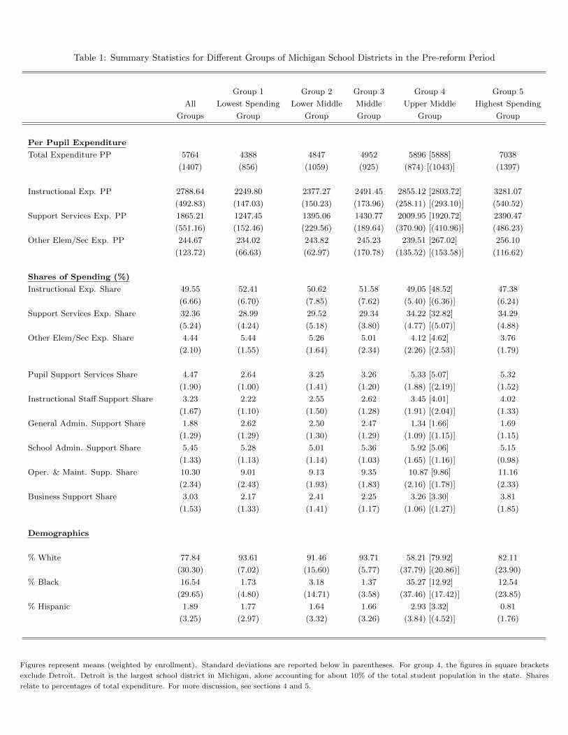
Table 1: Summary Statistics for Different Groups of Michigan School Districts in the Pre-reform Period

Group 1 Group 2 Group 3 Group 4 Group 5

All Lowest Spending Lower Middle Middle Upper Middle Highest Spending

Groups Group Group Group Group Group

Per Pupil Expenditure

Total Expenditure PP 5764 4388 4847 4952 5896 [5888] 7038

(1407) (856) (1059) (925) (874) [(1043)] (1397)

Instructional Exp. PP 2788.64 2249.80 2377.27 2491.45 2855.12 [2803.72] 3281.07

(492.83) (147.03) (150.23) (173.96) (258.11) [(293.10)] (540.52)

Support Services Exp. PP 1865.21 1247.45 1395.06 1430.77 2009.95 [1920.72] 2390.47

(551.16) (152.46) (229.56) (189.64) (370.90) [(410.96)] (486.23)

Other Elem/Sec Exp. PP 244.67 234.02 243.82 245.23 239.51 [267.02] 256.10

(123.72) (66.63) (62.97) (170.78) (135.52) [(153.58)] (116.62)

Shares of Spending (%)

Instructional Exp. Share 49.55 52.41 50.62 51.58 49.05 [48.52] 47.38

(6.66) (6.70) (7.85) (7.62) (5.40) [(6.36)] (6.24)

Support Services Exp. Share 32.36 28.99 29.52 29.34 34.22 [32.82] 34.29

(5.24) (4.24) (5.18) (3.80) (4.77) [(5.07)] (4.88)

Other Elem/Sec Exp. Share 4.44 5.44 5.26 5.01 4.12 [4.62] 3.76

(2.10) (1.55) (1.64) (2.34) (2.26) [(2.53)] (1.79)

Pupil Support Services Share 4.47 2.64 3.25 3.26 5.33 [5.07] 5.32

(1.90) (1.00) (1.41) (1.20) (1.88) [(2.19)] (1.52)

Instructional Staff Support Share 3.23 2.22 2.55 2.62 3.45 [4.01] 4.02

(1.67) (1.10) (1.50) (1.28) (1.91) [(2.04)] (1.33)

General Admin. Support Share 1.88 2.62 2.50 2.47 1.34 [1.66] 1.69

(1.29) (1.29) (1.30) (1.29) (1.09) [(1.15)] (1.15)

School Admin. Support Share 5.45 5.28 5.01 5.36 5.92 [5.06] 5.15

(1.33) (1.13) (1.14) (1.03) (1.65) [(1.16)] (0.98)

Oper. & Maint. Supp. Share 10.30 9.01 9.13 9.35 10.87 [9.86] 11.16

(2.34) (2.43) (1.93) (1.83) (2.16) [(1.78)] (2.33)

Business Support Share 3.03 2.17 2.41 2.25 3.26 [3.30] 3.81

(1.53) (1.33) (1.41) (1.17) (1.06) [(1.27)] (1.85)

Demographics

% White 77.84 93.61 91.46 93.71 58.21 [79.92] 82.11

(30.30) (7.02) (15.60) (5.77) (37.79) [(20.86)] (23.90)

% Black 16.54 1.73 3.18 1.37 35.27 [12.92] 12.54

(29.65) (4.80) (14.71) (3.58) (37.46) [(17.42)] (23.85)

% Hispanic 1.89 1.77 1.64 1.66 2.93 [3.32] 0.81

(3.25) (2.97) (3.32) (3.26) (3.84) [(4.52)] (1.76)

Figures represent means (weighted by enrollment). Standard deviations are reported below in parentheses. For group 4, the figures in square brackets

exclude Detroit. Detroit is the largest school district in Michigan, alone accounting for about 10% of the total student population in the state. Shares

relate to percentages of total expenditure. For more discussion, see sections 4 and 5.

1

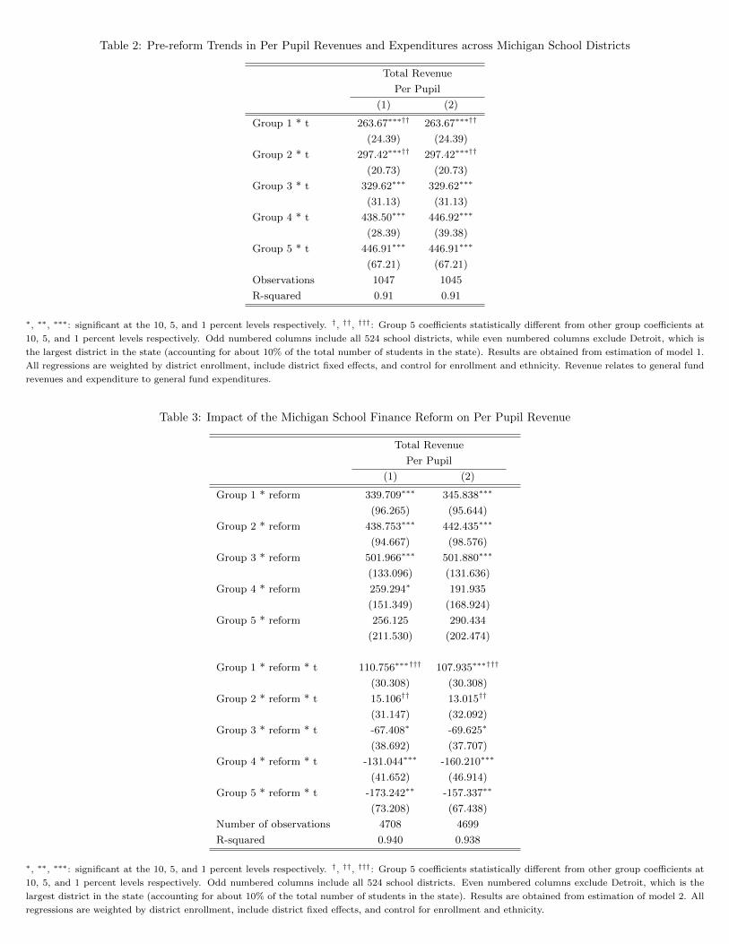
Table 2: Pre-reform Trends in Per Pupil Revenues and Expenditures across Michigan School Districts

Total Revenue

Per Pupil

(1) (2)

Group 1 * t 263.67∗∗∗†† 263.67∗∗∗††

(24.39) (24.39)

Group 2 * t 297.42∗∗∗†† 297.42∗∗∗††

(20.73) (20.73)

Group 3 * t 329.62∗∗∗ 329.62∗∗∗

(31.13) (31.13)

Group 4 * t 438.50∗∗∗ 446.92∗∗∗

(28.39) (39.38)

Group 5 * t 446.91∗∗∗ 446.91∗∗∗

(67.21) (67.21)

Observations 1047 1045

R-squared 0.91 0.91

∗, ∗∗, ∗∗∗: significant at the 10, 5, and 1 percent levels respectively. †, ††, †††: Group 5 coefficients statistically different from other group coefficients at

10, 5, and 1 percent levels respectively. Odd numbered columns include all 524 school districts, while even numbered columns exclude Detroit, which is

the largest district in the state (accounting for about 10% of the total number of students in the state). Results are obtained from estimation of model 1.

All regressions are weighted by district enrollment, include district fixed effects, and control for enrollment and ethnicity. Revenue relates to general fund

revenues and expenditure to general fund expenditures.

Table 3: Impact of the Michigan School Finance Reform on Per Pupil Revenue

Total Revenue

Per Pupil

(1) (2)

Group 1 * reform 339.709∗∗∗ 345.838∗∗∗

(96.265) (95.644)

Group 2 * reform 438.753∗∗∗ 442.435∗∗∗

(94.667) (98.576)

Group 3 * reform 501.966∗∗∗ 501.880∗∗∗

(133.096) (131.636)

Group 4 * reform 259.294∗ 191.935

(151.349) (168.924)

Group 5 * reform 256.125 290.434

(211.530) (202.474)

Group 1 * reform * t 110.756∗∗∗††† 107.935∗∗∗†††

(30.308) (30.308)

Group 2 * reform * t 15.106†† 13.015††

(31.147) (32.092)

Group 3 * reform * t -67.408∗ -69.625∗

(38.692) (37.707)

Group 4 * reform * t -131.044∗∗∗ -160.210∗∗∗

(41.652) (46.914)

Group 5 * reform * t -173.242∗∗ -157.337∗∗

(73.208) (67.438)

Number of observations 4708 4699

R-squared 0.940 0.938

∗, ∗∗, ∗∗∗: significant at the 10, 5, and 1 percent levels respectively. †, ††, †††: Group 5 coefficients statistically different from other group coefficients at

10, 5, and 1 percent levels respectively. Odd numbered columns include all 524 school districts. Even numbered columns exclude Detroit, which is the

largest district in the state (accounting for about 10% of the total number of students in the state). Results are obtained from estimation of model 2. All

regressions are weighted by district enrollment, include district fixed effects, and control for enrollment and ethnicity.

2

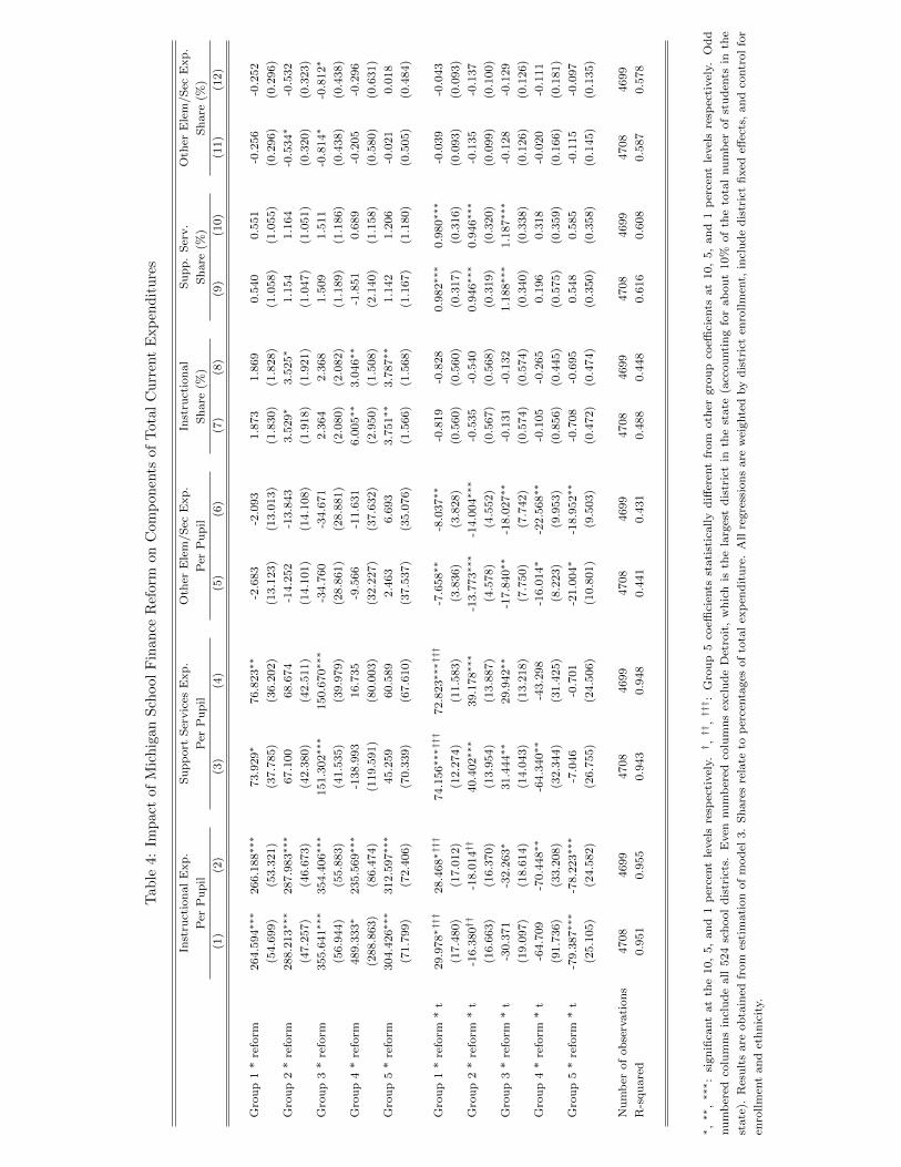
Tab

le4:

Imp

act

ofM

ich

igan

Sch

ool

Fin

an

ceR

eform

on

Com

pon

ents

of

Tota

lC

urr

ent

Exp

end

itu

res

Inst

ruct

ion

al

Exp

.S

up

port

Ser

vic

esE

xp

.O

ther

Ele

m/S

ecE

xp

.In

stru

ctio

nal

Su

pp

.S

erv.

Oth

erE

lem

/S

ecE

xp

.

Per

Pu

pil

Per

Pu

pil

Per

Pu

pil

Share

(%)

Sh

are

(%)

Sh

are

(%)

(1)

(2)

(3)

(4)

(5)

(6)

(7)

(8)

(9)

(10)

(11)

(12)

Gro

up

1*

refo

rm264.5

94∗∗∗

266.1

88∗∗∗

73.9

29∗

76.8

23∗∗

-2.6

83

-2.0

93

1.8

73

1.8

69

0.5

40

0.5

51

-0.2

56

-0.2

52

(54.6

99)

(53.3

21)

(37.7

85)

(36.2

02)

(13.1

23)

(13.0

13)

(1.8

30)

(1.8

28)

(1.0

58)

(1.0

55)

(0.2

96)

(0.2

96)

Gro

up

2*

refo

rm288.2

13∗∗∗

287.9

83∗∗∗

67.1

00

68.6

74

-14.2

52

-13.8

43

3.5

29∗

3.5

25∗

1.1

54

1.1

64

-0.5

34∗

-0.5

32

(47.2

57)

(46.6

73)

(42.3

80)

(42.5

11)

(14.1

01)

(14.1

08)

(1.9

18)

(1.9

21)

(1.0

47)

(1.0

51)

(0.3

20)

(0.3

23)

Gro

up

3*

refo

rm355.6

41∗∗∗

354.4

06∗∗∗

151.3

02∗∗∗

150.6

70∗∗∗

-34.7

60

-34.6

71

2.3

64

2.3

68

1.5

09

1.5

11

-0.8

14∗

-0.8

12∗

(56.9

44)

(55.8

83)

(41.5

35)

(39.9

79)

(28.8

61)

(28.8

81)

(2.0

80)

(2.0

82)

(1.1

89)

(1.1

86)

(0.4

38)

(0.4

38)

Gro

up

4*

refo

rm489.3

33∗

235.5

69∗∗∗

-138.9

93

16.7

35

-9.5

66

-11.6

31

6.0

05∗∗

3.0

46∗∗

-1.8

51

0.6

89

-0.2

05

-0.2

96

(288.8

63)

(86.4

74)

(119.5

91)

(80.0

03)

(32.2

27)

(37.6

32)

(2.9

50)

(1.5

08)

(2.1

40)

(1.1

58)

(0.5

80)

(0.6

31)

Gro

up

5*

refo

rm304.4

26∗∗∗

312.5

97∗∗∗

45.2

59

60.5

89

2.4

63

6.6

93

3.7

51∗∗

3.7

87∗∗

1.1

42

1.2

06

-0.0

21

0.0

18

(71.7

99)

(72.4

06)

(70.3

39)

(67.6

10)

(37.5

37)

(35.0

76)

(1.5

66)

(1.5

68)

(1.1

67)

(1.1

80)

(0.5

05)

(0.4

84)

Gro

up

1*

refo

rm*

t29.9

78∗†††

28.4

68∗†††

74.1

56∗∗∗†††

72.8

23∗∗∗†††

-7.6

58∗∗

-8.0

37∗∗

-0.8

19

-0.8

28

0.9

82∗∗∗

0.9

80∗∗∗

-0.0

39

-0.0

43

(17.4

80)

(17.0

12)

(12.2

74)

(11.5

83)

(3.8

36)

(3.8

28)

(0.5

60)

(0.5

60)

(0.3

17)

(0.3

16)

(0.0

93)

(0.0

93)

Gro

up

2*

refo

rm*

t-1

6.3

80††

-18.0

14††

40.4

02∗∗∗

39.1

78∗∗∗

-13.7

73∗∗∗

-14.0

04∗∗∗

-0.5

35

-0.5

40

0.9

46∗∗∗

0.9

46∗∗∗

-0.1

35

-0.1

37

(16.6

63)

(16.3

70)

(13.9

54)

(13.8

87)

(4.5

78)

(4.5

52)

(0.5

67)

(0.5

68)

(0.3

19)

(0.3

20)

(0.0

99)

(0.1

00)

Gro

up

3*

refo

rm*

t-3

0.3

71

-32.2

63∗

31.4

44∗∗

29.9

42∗∗

-17.8

40∗∗

-18.0

27∗∗

-0.1

31

-0.1

32

1.1

88∗∗∗

1.1

87∗∗∗

-0.1

28

-0.1

29

(19.0

97)

(18.6

14)

(14.0

43)

(13.2

18)

(7.7

50)

(7.7

42)

(0.5

74)

(0.5

74)

(0.3

40)

(0.3

38)

(0.1

26)

(0.1

26)

Gro

up

4*

refo

rm*

t-6

4.7

09

-70.4

48∗∗

-64.3

40∗∗

-43.2

98

-16.0

14∗

-22.5

68∗∗

-0.1

05

-0.2

65

0.1

96

0.3

18

-0.0

20

-0.1

11

(91.7

36)

(33.2

08)

(32.3

44)

(31.4

25)

(8.2

23)

(9.9

53)

(0.8

56)

(0.4

45)

(0.5

75)

(0.3

59)

(0.1

66)

(0.1

81)

Gro

up

5*

refo

rm*

t-7

9.3

87∗∗∗

-78.2

23∗∗∗

-7.0

46

-0.7

01

-21.0

04∗

-18.9

52∗∗

-0.7

08

-0.6

95

0.5

48

0.5

85

-0.1

15

-0.0

97

(25.1

05)

(24.5

82)

(26.7

55)

(24.5

06)

(10.8

01)

(9.5

03)

(0.4

72)

(0.4

74)

(0.3

50)

(0.3

58)

(0.1

45)

(0.1

35)

Nu

mb

erof

ob

serv

ati

on

s4708

4699

4708

4699

4708

4699

4708

4699

4708

4699

4708

4699

R-s

qu

are

d0.9

51

0.9

55

0.9

43

0.9

48

0.4

41

0.4

31

0.4

88

0.4

48

0.6

16

0.6

08

0.5

87

0.5

78

∗,∗∗

,∗∗∗:

sign

ifica

nt

at

the

10,

5,

an

d1

per

cent

level

sre

spec

tivel

y.† ,††

,††† :

Gro

up

5co

effici

ents

stati

stic

ally

diff

eren

tfr

om

oth

ergro

up

coeffi

cien

tsat

10,

5,

an

d1

per

cent

level

sre

spec

tivel

y.O

dd

nu

mb

ered

colu

mn

sin

clu

de

all

524

sch

ool

dis

tric

ts.

Even

nu

mb

ered

colu

mn

sex

clu

de

Det

roit

,w

hic

his

the

larg

est

dis

tric

tin

the

state

(acc

ou

nti

ng

for

ab

ou

t10%

of

the

tota

lnu

mb

erof

stu

den

tsin

the

state

).R

esu

lts

are

ob

tain

edfr

om

esti

mati

on

of

mod

el3.

Sh

are

sre

late

top

erce

nta

ges

of

tota

lex

pen

dit

ure

.A

llre

gre

ssio

ns

are

wei

ghte

dby

dis

tric

ten

rollm

ent,

incl

ud

ed

istr

ict

fixed

effec

ts,

an

dco

ntr

ol

for

enro

llm

ent

an

det

hn

icit

y.

3

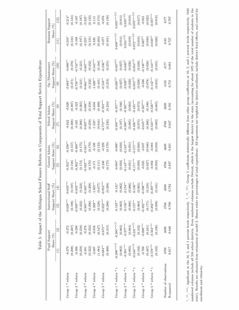
Tab

le5:

Imp

act

ofth

eM

ich

igan

Sch

ool

Fin

an

ceR

eform

on

Com

pon

ents

of

Tota

lS

up

port

Ser

vic

eE

xp

end

itu

re

Pu

pil

Su

pp

ort

Inst

ruct

ion

al

Sta

ffG

ener

al

Ad

min

.S

chool

Ad

min

.O

p./

Main

ten

an

ceB

usi

nes

sS

up

port

Sh

are

(%)

Su

pp

ort

Sh

are

(%)

Su

pp

ort

Sh

are

(%)

Su

pp

ort

Sh

are

(%)

Su

pp

ort

Sh

are

(%)

Sh

are

(%)

(1)

(2)

(3)

(4)

(5)

(6)

(7)

(8)

(9)

(10)

(11)

(12)

Gro

up

1*

refo

rm-0

.279

-0.2

72

-0.6

28∗∗∗

-0.6

33∗∗∗

-0.3

52∗∗

-0.3

50∗∗

-0.6

22

-0.6

20

-0.6

83∗∗

-0.6

86∗∗

-0.2

16∗

-0.2

14∗

(0.2

08)

(0.2

07)

(0.1

98)

(0.1

97)

(0.1

58)

(0.1

57)

(0.3

88)

(0.3

87)

(0.2

71)

(0.2

70)

(0.1

24)

(0.1

24)

Gro

up

2*

refo

rm-0

.306

-0.2

98

-0.9

30∗∗∗

-0.9

33∗∗∗

-0.3

62∗∗

-0.3

60∗∗

-0.3

25

-0.3

22

-0.7

39∗∗∗

-0.7

42∗∗∗

-0.1

69

-0.1

67

(0.2

59)

(0.2

58)

(0.2

22)

(0.2

23)

(0.1

74)

(0.1

75)

(0.2

66)

(0.2

65)

(0.2

21)

(0.2

21)

(0.1

97)

(0.1

97)

Gro

up

3*

refo

rm-0

.281

-0.2

78

-0.5

65∗∗∗

-0.5

65∗∗∗

-0.5

82∗∗∗

-0.5

81∗∗∗

-0.6

07∗∗

-0.6

06∗∗

-0.6

64∗∗∗

-0.6

67∗∗∗

-0.2

25∗

-0.2

25∗

(0.3

22)

(0.3

22)

(0.2

06)

(0.2

09)

(0.1

70)

(0.1

70)

(0.2

59)

(0.2

58)

(0.2

32)

(0.2

32)

(0.1

21)

(0.1

22)

Gro

up

4*

refo

rm-2

.087

-0.8

58

-1.2

08∗∗

-1.6

01∗∗

-0.1

71

-0.1

98

-1.5

35∗

-0.6

58

-1.0

26∗∗

-0.5

43∗∗∗

0.3

49

0.1

13

(1.4

84)

(0.5

47)

(0.5

28)

(0.6

77)

(0.1

11)

(0.1

33)

(0.8

44)

(0.4

09)

(0.4

41)

(0.1

94)

(0.3

93)

(0.1

74)

Gro

up

5*

refo

rm-0

.684∗∗

-0.6

75∗∗

-0.9

22∗∗∗

-0.9

52∗∗∗

-0.2

46

-0.2

29

-0.7

72∗∗∗

-0.7

63∗∗∗

-0.5

34∗∗

-0.5

36∗∗

-0.0

77

-0.0

76

(0.3

09)

(0.3

15)

(0.2

80)

(0.2

89)

(0.1

75)

(0.1

78)

(0.2

32)

(0.2

34)

(0.2

53)

(0.2

55)

(0.1

61)

(0.1

58)

Gro

up

1*

refo

rm*

t-0

.290∗∗∗††

-0.2

85∗∗∗††

-0.1

23∗∗

-0.1

21∗

-0.0

84∗

-0.0

86∗

-0.3

58∗∗∗

-0.3

57∗∗∗

-0.0

26†††

-0.0

27†††

0.0

38∗∗∗†††

0.0

35∗∗∗†††

(0.0

63)

(0.0

62)

(0.0

63)

(0.0

62)

(0.0

50)

(0.0

50)

(0.1

07)

(0.1

06)

(0.0

27)

(0.0

27)

(0.0

14)

(0.0

14)

Gro

up

2*

refo

rm*

t-0

.381∗∗∗

-0.3

77∗∗∗

-0.1

56∗∗

-0.1

54∗∗

-0.1

43∗∗∗

-0.1

43∗∗∗

-0.3

88∗∗∗

-0.3

87∗∗∗

-0.0

39††

-0.0

40††

0.0

34∗†††

0.0

33∗†††

(0.0

85)

(0.0

84)

(0.0

66)

(0.0

66)

(0.0

51)

(0.0

51)

(0.0

85)

(0.0

84)

(0.0

30)

(0.0

30)

(0.0

19)

(0.0

19)

Gro

up

3*

refo

rm*

t-0

.244∗∗††

-0.2

41∗∗††

-0.1

37∗∗

-0.1

36∗∗

-0.1

71∗∗∗

-0.1

71∗∗∗

-0.4

36∗∗∗

-0.4

35∗∗∗

-0.0

53∗††

-0.0

54∗††

0.0

72∗∗∗†††

0.0

70∗∗∗†††

(0.1

02)

(0.1

02)

(0.0

64)

(0.0

65)

(0.0

50)

(0.0

50)

(0.0

74)

(0.0

73)

(0.0

28)

(0.0

28)

(0.0

18)

(0.0

17)

Gro

up

4*

refo

rm*

t-0

.766

-0.6

96∗∗∗

-0.4

82∗∗∗

-0.5

96∗∗∗

-0.0

25

-0.0

47

-0.6

45∗∗

-0.5

67∗∗∗

-0.0

46

-0.1

46∗∗∗

0.0

67††

-0.0

21

(0.4

87)

(0.2

41)

(0.1

71)

(0.2

16)

(0.0

37)

(0.0

46)

(0.2

66)

(0.1

86)

(0.0

78)

(0.0

26)

(0.0

49)

(0.0

22)

Gro

up

5*

refo

rm*

t-0

.578∗∗∗

-0.5

64∗∗∗

-0.2

82∗∗∗

-0.2

97∗∗∗

-0.0

92

-0.0

83

-0.5

34∗∗∗

-0.5

26∗∗∗

-0.1

42∗∗∗

-0.1

43∗∗∗

-0.0

49∗∗

-0.0

57∗∗∗

(0.1

02)

(0.1

06)

(0.0

99)

(0.1

01)

(0.0

59)

(0.0

59)

(0.0

83)

(0.0

85)

(0.0

31)

(0.0

31)

(0.0

20)

(0.0

18)

Nu

mb

erof

ob

serv

ati

on

s4708

4699

4708

4699

4708

4699

4708

4699

4185

4177

4185

4177

R-s

qu

are

d0.8

17

0.8

46

0.7

89

0.7

82

0.8

37

0.8

21

0.6

47

0.5

91

0.7

31

0.6

81

0.7

27

0.7

07

∗,∗∗

,∗∗∗:

sign

ifica

nt

at

the

10,

5,

an

d1

per

cent

level

sre

spec

tivel

y.† ,††

,††† :

Gro

up

5co

effici

ents

stati

stic

ally

diff

eren

tfr

om

oth

ergro

up

coeffi

cien

tsat

10,

5,

an

d1

per

cent

level

sre

spec

tivel

y.O

dd

nu

mb

ered

colu

mn

sin

clu

de

all

524

sch

ool

dis

tric

ts.

Even

nu

mb

ered

colu

mn

sex

clu

de

Det

roit

,w

hic

his

the

larg

est

dis

tric

tin

the

state

(acc

ou

nti

ng

for

ab

ou

t10%

of

the

tota

lnu

mb

erof

stu

den

tsin

the

state

).R

esu

lts

are

ob

tain

edfr

om

esti

mati

on

of

mod

el3.

Sh

are

sre

late

top

erce

nta

ges

of

tota

lex

pen

dit

ure

.A

llre

gre

ssio

ns

are

wei

ghte

dby

dis

tric

ten

rollm

ent,

incl

ud

ed

istr

ict

fixed

effec

ts,

an

dco

ntr

ol

for

enro

llm

ent

an

det

hn

icit

y.

4

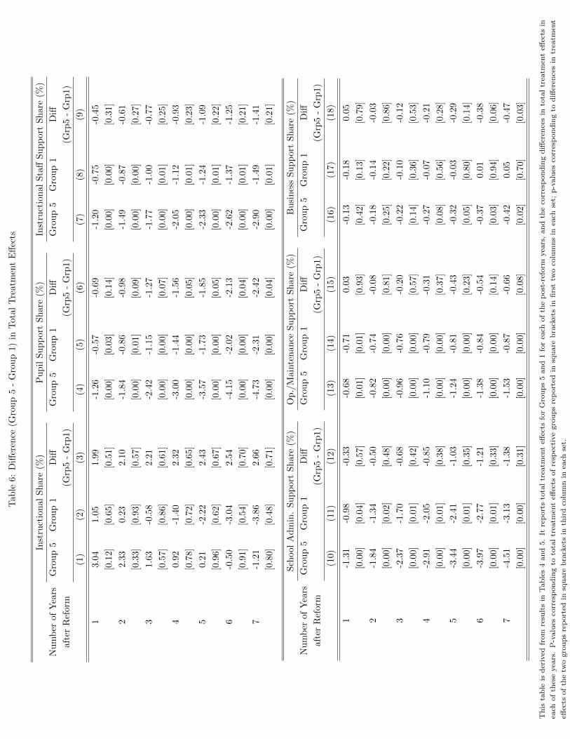
Tab

le6:

Diff

eren

ce(G

rou

p5

-G

rou

p1)

inT

ota

lT

reatm

ent

Eff

ects

Inst

ruct

ion

alS

har

e(%

)P

up

ilS

up

port

Share

(%)

Inst

ruct

ion

al

Sta

ffS

up

port

Sh

are

(%)

Nu

mb

erof

Yea

rsG

rou

p5

Gro

up

1D

iffG

rou

p5

Gro

up

1D

iffG

rou

p5

Gro

up

1D

iff

afte

rR

efor

m(G

rp5

-G

rp1)

(Grp

5-

Grp

1)

(Grp

5-

Grp

1)

(1)

(2)

(3)

(4)

(5)

(6)

(7)

(8)

(9)

13.

041.

051.9

9-1

.26

-0.5

7-0

.69

-1.2

0-0

.75

-0.4

5

[0.1

2][0

.65]

[0.5

1]

[0.0

0]

[0.0

3]

[0.1

4]

[0.0

0]

[0.0

0]

[0.3

1]

22.

330.

232.1

0-1

.84

-0.8

6-0

.98

-1.4

9-0

.87

-0.6

1

[0.3

3][0

.93]

[0.5

7]

[0.0

0]

[0.0

1]

[0.0

9]

[0.0

0]

[0.0

0]

[0.2

7]

31.

63-0

.58

2.2

1-2

.42

-1.1

5-1

.27

-1.7

7-1

.00

-0.7

7

[0.5

7][0

.86]

[0.6

1]

[0.0

0]

[0.0

0]

[0.0

7]

[0.0

0]

[0.0

1]

[0.2

5]

40.

92-1

.40

2.3

2-3

.00

-1.4

4-1

.56

-2.0

5-1

.12

-0.9

3

[0.7

8][0

.72]

[0.6

5]

[0.0

0]

[0.0

0]

[0.0

5]

[0.0

0]

[0.0

1]

[0.2

3]

50.

21-2

.22

2.4

3-3

.57

-1.7

3-1

.85

-2.3

3-1

.24

-1.0

9

[0.9

6][0

.62]

[0.6

7]

[0.0

0]

[0.0

0]

[0.0

5]

[0.0

0]

[0.0

1]

[0.2

2]

6-0

.50

-3.0

42.5

4-4

.15

-2.0

2-2

.13

-2.6

2-1

.37

-1.2

5

[0.9

1][0

.54]

[0.7

0]

[0.0

0]

[0.0

0]

[0.0

4]

[0.0

0]

[0.0

1]

[0.2

1]

7-1

.21

-3.8

62.6

6-4

.73

-2.3

1-2

.42

-2.9

0-1

.49

-1.4

1

[0.8

0][0

.48]

[0.7

1]

[0.0

0]

[0.0

0]

[0.0

4]

[0.0

0]

[0.0

1]

[0.2

1]

Sch

ool

Ad

min

.S

up

por

tS

hare

(%)

Op

./M

ain

ten

an

ceS

up

port

Sh

are

(%)

Bu

sin

ess

Su

pp

ort

Sh

are

(%)

Nu

mb

erof

Yea

rsG

rou

p5

Gro

up

1D

iffG

roup

5G

rou

p1

Diff

Gro

up

5G

rou

p1

Diff

afte

rR

efor

m(G

rp5

-G

rp1)

(Grp

5-

Grp

1)(G

rp5

-G

rp1)

(10)

(11)

(12)

(13)

(14)

(15)

(16)

(17)

(18)

1-1

.31

-0.9

8-0

.33

-0.6

8-0

.71

0.0

3-0

.13

-0.1

80.0

5

[0.0

0][0

.04]

[0.5

7]

[0.0

1]

[0.0

1]

[0.9

3]

[0.4

2]

[0.1

3]

[0.7

9]

2-1

.84

-1.3

4-0

.50

-0.8

2-0

.74

-0.0

8-0

.18

-0.1

4-0

.03

[0.0

0][0

.02]

[0.4

8]

[0.0

0]

[0.0

0]

[0.8

1]

[0.2

5]

[0.2

2]

[0.8

6]

3-2

.37

-1.7

0-0

.68

-0.9

6-0

.76

-0.2

0-0

.22

-0.1

0-0

.12

[0.0

0][0

.01]

[0.4

2]

[0.0

0]

[0.0

0]

[0.5

7]

[0.1

4]

[0.3

6]

[0.5

3]

4-2

.91

-2.0

5-0

.85

-1.1

0-0

.79

-0.3

1-0

.27

-0.0

7-0

.21

[0.0

0][0

.01]

[0.3

8]

[0.0

0]

[0.0

0]

[0.3

7]

[0.0

8]

[0.5

6]

[0.2

8]

5-3

.44

-2.4

1-1

.03

-1.2

4-0

.81

-0.4

3-0

.32

-0.0

3-0

.29

[0.0

0][0

.01]

[0.3

5]

[0.0

0]

[0.0

0]

[0.2

3]

[0.0

5]

[0.8

0]

[0.1

4]

6-3

.97

-2.7

7-1

.21

-1.3

8-0

.84

-0.5

4-0

.37

0.0

1-0

.38

[0.0

0][0

.01]

[0.3

3]

[0.0

0]

[0.0

0]

[0.1

4]

[0.0

3]

[0.9

4]

[0.0

6]

7-4

.51

-3.1

3-1

.38

-1.5

3-0

.87

-0.6

6-0

.42

0.0

5-0

.47

[0.0

0][0

.00]

[0.3

1]

[0.0

0]

[0.0

0]

[0.0

8]

[0.0

2]

[0.7

0]

[0.0

3]

Th

ista

ble

isd

eriv

edfr

om

resu

lts

inT

ab

les

4an

d5.

Itre

port

sto

tal

trea

tmen

teff

ects

for

Gro

up

s5

an

d1

for

each

of

the

post

-ref

orm

yea

rs,

an

dth

eco

rres

pon

din

gd

iffer

ence

sin

tota

ltr

eatm

ent

effec

tsin

each

of

thes

eyea

rs.

P-v

alu

esco

rres

pon

din

gto

tota

ltr

eatm

ent

effec

tsof

resp

ecti

ve

gro

ups

rep

ort

edin

squ

are

bra

cket

sin

firs

ttw

oco

lum

ns

inea

chse

t;p

-valu

esco

rres

pon

din

gto

diff

eren

ces

intr

eatm

ent

effec

tsof

the

two

gro

up

sre

port

edin

squ

are

bra

cket

sin

thir

dco

lum

nin

each

set.

5

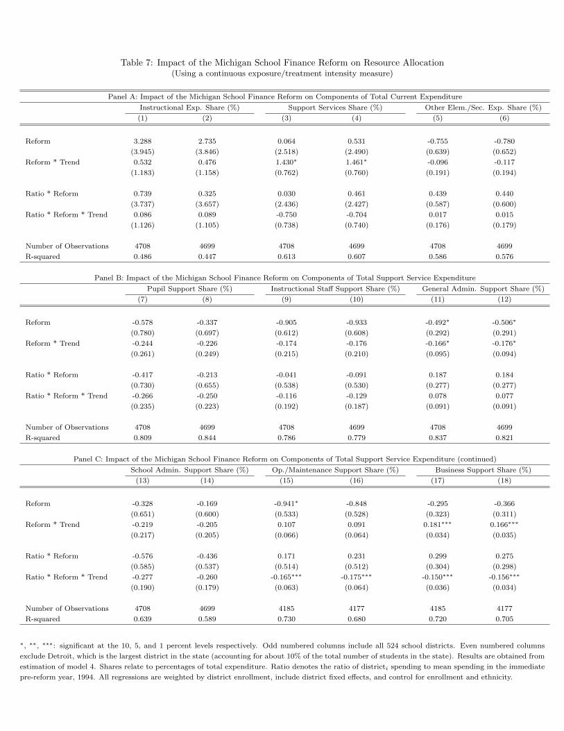
Table 7: Impact of the Michigan School Finance Reform on Resource Allocation(Using a continuous exposure/treatment intensity measure)

Panel A: Impact of the Michigan School Finance Reform on Components of Total Current Expenditure

Instructional Exp. Share (%) Support Services Share (%) Other Elem./Sec. Exp. Share (%)

(1) (2) (3) (4) (5) (6)

Reform 3.288 2.735 0.064 0.531 -0.755 -0.780

(3.945) (3.846) (2.518) (2.490) (0.639) (0.652)

Reform * Trend 0.532 0.476 1.430∗ 1.461∗ -0.096 -0.117

(1.183) (1.158) (0.762) (0.760) (0.191) (0.194)

Ratio * Reform 0.739 0.325 0.030 0.461 0.439 0.440

(3.737) (3.657) (2.436) (2.427) (0.587) (0.600)

Ratio * Reform * Trend 0.086 0.089 -0.750 -0.704 0.017 0.015

(1.126) (1.105) (0.738) (0.740) (0.176) (0.179)

Number of Observations 4708 4699 4708 4699 4708 4699

R-squared 0.486 0.447 0.613 0.607 0.586 0.576

Panel B: Impact of the Michigan School Finance Reform on Components of Total Support Service Expenditure

Pupil Support Share (%) Instructional Staff Support Share (%) General Admin. Support Share (%)

(7) (8) (9) (10) (11) (12)

Reform -0.578 -0.337 -0.905 -0.933 -0.492∗ -0.506∗

(0.780) (0.697) (0.612) (0.608) (0.292) (0.291)

Reform * Trend -0.244 -0.226 -0.174 -0.176 -0.166∗ -0.176∗

(0.261) (0.249) (0.215) (0.210) (0.095) (0.094)

Ratio * Reform -0.417 -0.213 -0.041 -0.091 0.187 0.184

(0.730) (0.655) (0.538) (0.530) (0.277) (0.277)

Ratio * Reform * Trend -0.266 -0.250 -0.116 -0.129 0.078 0.077

(0.235) (0.223) (0.192) (0.187) (0.091) (0.091)

Number of Observations 4708 4699 4708 4699 4708 4699

R-squared 0.809 0.844 0.786 0.779 0.837 0.821

Panel C: Impact of the Michigan School Finance Reform on Components of Total Support Service Expenditure (continued)

School Admin. Support Share (%) Op./Maintenance Support Share (%) Business Support Share (%)

(13) (14) (15) (16) (17) (18)

Reform -0.328 -0.169 -0.941∗ -0.848 -0.295 -0.366

(0.651) (0.600) (0.533) (0.528) (0.323) (0.311)

Reform * Trend -0.219 -0.205 0.107 0.091 0.181∗∗∗ 0.166∗∗∗

(0.217) (0.205) (0.066) (0.064) (0.034) (0.035)

Ratio * Reform -0.576 -0.436 0.171 0.231 0.299 0.275

(0.585) (0.537) (0.514) (0.512) (0.304) (0.298)

Ratio * Reform * Trend -0.277 -0.260 -0.165∗∗∗ -0.175∗∗∗ -0.150∗∗∗ -0.156∗∗∗

(0.190) (0.179) (0.063) (0.064) (0.036) (0.034)

Number of Observations 4708 4699 4185 4177 4185 4177

R-squared 0.639 0.589 0.730 0.680 0.720 0.705

∗, ∗∗, ∗∗∗: significant at the 10, 5, and 1 percent levels respectively. Odd numbered columns include all 524 school districts. Even numbered columns

exclude Detroit, which is the largest district in the state (accounting for about 10% of the total number of students in the state). Results are obtained from

estimation of model 4. Shares relate to percentages of total expenditure. Ratio denotes the ratio of districti spending to mean spending in the immediate

pre-reform year, 1994. All regressions are weighted by district enrollment, include district fixed effects, and control for enrollment and ethnicity.

6

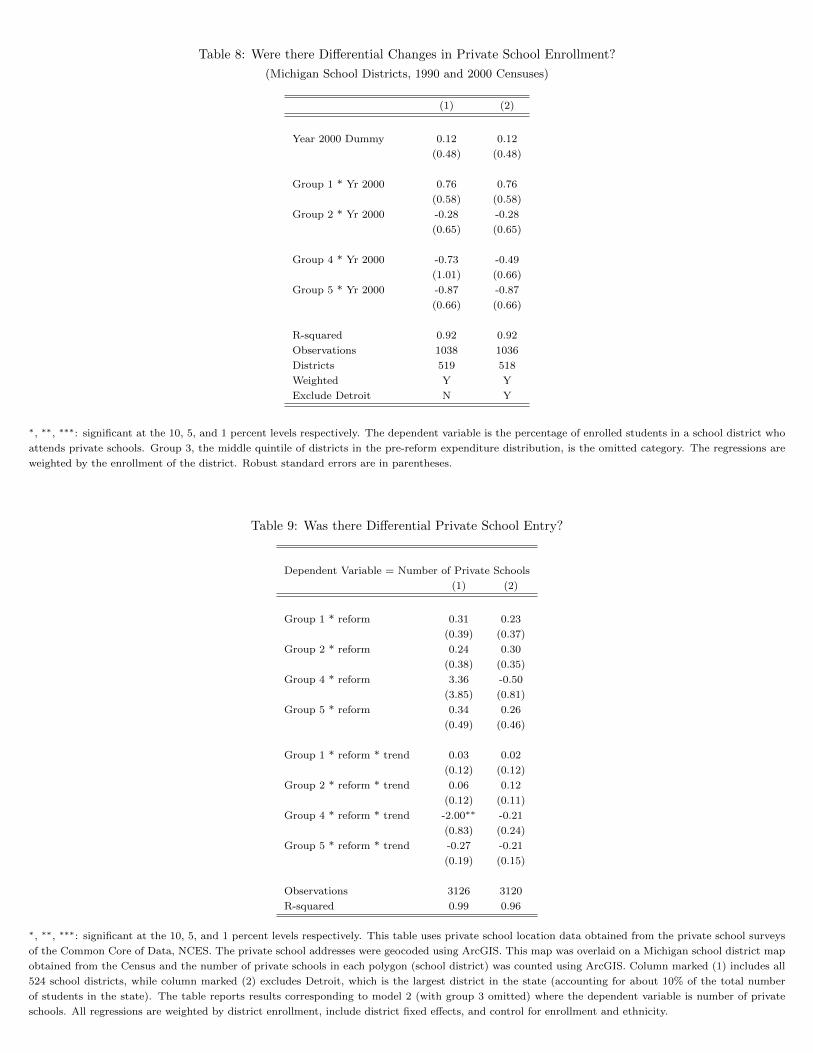
Table 8: Were there Differential Changes in Private School Enrollment?

(Michigan School Districts, 1990 and 2000 Censuses)

(1) (2)

Year 2000 Dummy 0.12 0.12

(0.48) (0.48)

Group 1 * Yr 2000 0.76 0.76

(0.58) (0.58)

Group 2 * Yr 2000 -0.28 -0.28

(0.65) (0.65)

Group 4 * Yr 2000 -0.73 -0.49

(1.01) (0.66)

Group 5 * Yr 2000 -0.87 -0.87

(0.66) (0.66)

R-squared 0.92 0.92

Observations 1038 1036

Districts 519 518

Weighted Y Y

Exclude Detroit N Y

∗, ∗∗, ∗∗∗: significant at the 10, 5, and 1 percent levels respectively. The dependent variable is the percentage of enrolled students in a school district who

attends private schools. Group 3, the middle quintile of districts in the pre-reform expenditure distribution, is the omitted category. The regressions are

weighted by the enrollment of the district. Robust standard errors are in parentheses.

Table 9: Was there Differential Private School Entry?

Dependent Variable = Number of Private Schools

(1) (2)

Group 1 * reform 0.31 0.23

(0.39) (0.37)

Group 2 * reform 0.24 0.30

(0.38) (0.35)

Group 4 * reform 3.36 -0.50

(3.85) (0.81)

Group 5 * reform 0.34 0.26

(0.49) (0.46)

Group 1 * reform * trend 0.03 0.02

(0.12) (0.12)

Group 2 * reform * trend 0.06 0.12

(0.12) (0.11)

Group 4 * reform * trend -2.00∗∗ -0.21

(0.83) (0.24)

Group 5 * reform * trend -0.27 -0.21

(0.19) (0.15)

Observations 3126 3120

R-squared 0.99 0.96

∗, ∗∗, ∗∗∗: significant at the 10, 5, and 1 percent levels respectively. This table uses private school location data obtained from the private school surveys

of the Common Core of Data, NCES. The private school addresses were geocoded using ArcGIS. This map was overlaid on a Michigan school district map

obtained from the Census and the number of private schools in each polygon (school district) was counted using ArcGIS. Column marked (1) includes all

524 school districts, while column marked (2) excludes Detroit, which is the largest district in the state (accounting for about 10% of the total number

of students in the state). The table reports results corresponding to model 2 (with group 3 omitted) where the dependent variable is number of private

schools. All regressions are weighted by district enrollment, include district fixed effects, and control for enrollment and ethnicity.

7

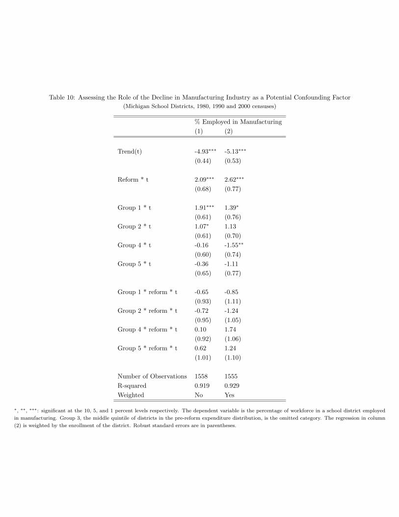
Table 10: Assessing the Role of the Decline in Manufacturing Industry as a Potential Confounding Factor

(Michigan School Districts, 1980, 1990 and 2000 censuses)

% Employed in Manufacturing

(1) (2)

Trend(t) -4.93∗∗∗ -5.13∗∗∗

(0.44) (0.53)

Reform * t 2.09∗∗∗ 2.62∗∗∗

(0.68) (0.77)

Group 1 * t 1.91∗∗∗ 1.39∗

(0.61) (0.76)

Group 2 * t 1.07∗ 1.13

(0.61) (0.70)

Group 4 * t -0.16 -1.55∗∗

(0.60) (0.74)

Group 5 * t -0.36 -1.11

(0.65) (0.77)

Group 1 * reform * t -0.65 -0.85

(0.93) (1.11)

Group 2 * reform * t -0.72 -1.24

(0.95) (1.05)

Group 4 * reform * t 0.10 1.74

(0.92) (1.06)

Group 5 * reform * t 0.62 1.24

(1.01) (1.10)

Number of Observations 1558 1555

R-squared 0.919 0.929

Weighted No Yes

∗, ∗∗, ∗∗∗: significant at the 10, 5, and 1 percent levels respectively. The dependent variable is the percentage of workforce in a school district employed

in manufacturing. Group 3, the middle quintile of districts in the pre-reform expenditure distribution, is the omitted category. The regression in column

(2) is weighted by the enrollment of the district. Robust standard errors are in parentheses.

8

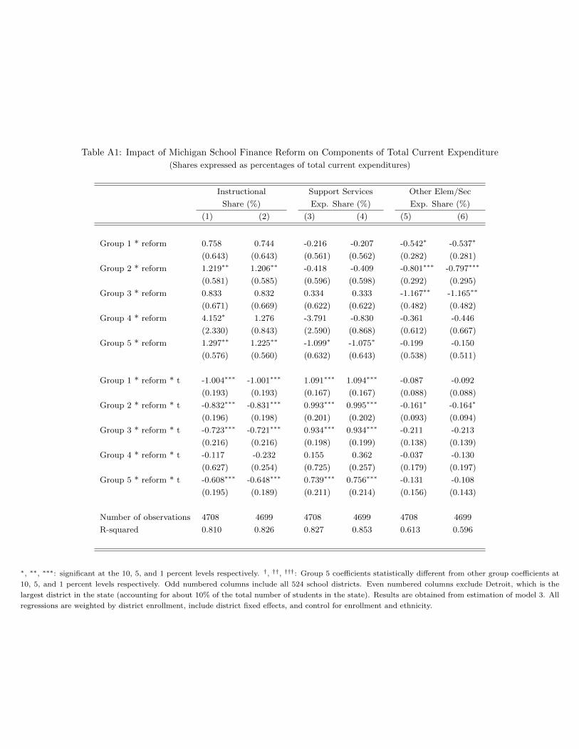
Table A1: Impact of Michigan School Finance Reform on Components of Total Current Expenditure

(Shares expressed as percentages of total current expenditures)

Instructional Support Services Other Elem/Sec

Share (%) Exp. Share (%) Exp. Share (%)

(1) (2) (3) (4) (5) (6)

Group 1 * reform 0.758 0.744 -0.216 -0.207 -0.542∗ -0.537∗

(0.643) (0.643) (0.561) (0.562) (0.282) (0.281)

Group 2 * reform 1.219∗∗ 1.206∗∗ -0.418 -0.409 -0.801∗∗∗ -0.797∗∗∗

(0.581) (0.585) (0.596) (0.598) (0.292) (0.295)

Group 3 * reform 0.833 0.832 0.334 0.333 -1.167∗∗ -1.165∗∗

(0.671) (0.669) (0.622) (0.622) (0.482) (0.482)

Group 4 * reform 4.152∗ 1.276 -3.791 -0.830 -0.361 -0.446

(2.330) (0.843) (2.590) (0.868) (0.612) (0.667)

Group 5 * reform 1.297∗∗ 1.225∗∗ -1.099∗ -1.075∗ -0.199 -0.150

(0.576) (0.560) (0.632) (0.643) (0.538) (0.511)

Group 1 * reform * t -1.004∗∗∗ -1.001∗∗∗ 1.091∗∗∗ 1.094∗∗∗ -0.087 -0.092

(0.193) (0.193) (0.167) (0.167) (0.088) (0.088)

Group 2 * reform * t -0.832∗∗∗ -0.831∗∗∗ 0.993∗∗∗ 0.995∗∗∗ -0.161∗ -0.164∗

(0.196) (0.198) (0.201) (0.202) (0.093) (0.094)

Group 3 * reform * t -0.723∗∗∗ -0.721∗∗∗ 0.934∗∗∗ 0.934∗∗∗ -0.211 -0.213

(0.216) (0.216) (0.198) (0.199) (0.138) (0.139)

Group 4 * reform * t -0.117 -0.232 0.155 0.362 -0.037 -0.130

(0.627) (0.254) (0.725) (0.257) (0.179) (0.197)

Group 5 * reform * t -0.608∗∗∗ -0.648∗∗∗ 0.739∗∗∗ 0.756∗∗∗ -0.131 -0.108

(0.195) (0.189) (0.211) (0.214) (0.156) (0.143)

Number of observations 4708 4699 4708 4699 4708 4699

R-squared 0.810 0.826 0.827 0.853 0.613 0.596

∗, ∗∗, ∗∗∗: significant at the 10, 5, and 1 percent levels respectively. †, ††, †††: Group 5 coefficients statistically different from other group coefficients at

10, 5, and 1 percent levels respectively. Odd numbered columns include all 524 school districts. Even numbered columns exclude Detroit, which is the

largest district in the state (accounting for about 10% of the total number of students in the state). Results are obtained from estimation of model 3. All

regressions are weighted by district enrollment, include district fixed effects, and control for enrollment and ethnicity.

9

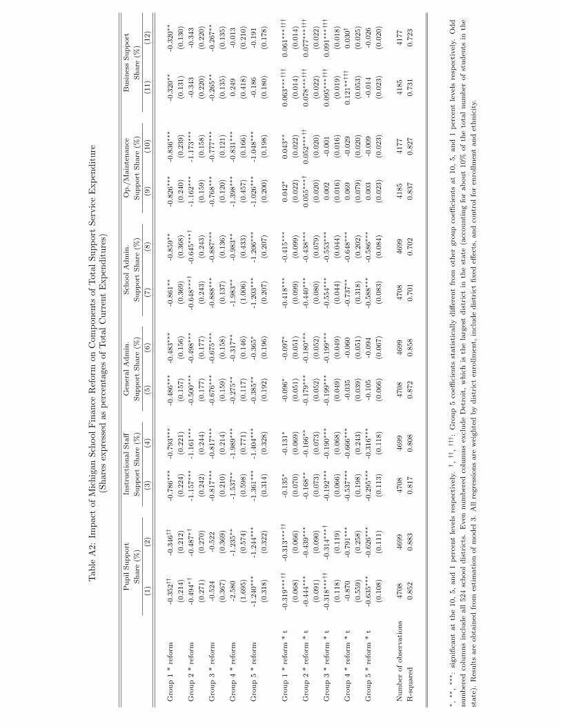
Tab

leA

2:Im

pac

tof

Mic

hig

an

Sch

ool

Fin

an

ceR

eform

on

Com

pon

ents

of

Tota

lS

up

port

Ser

vic

eE

xp

end

itu

re(S

har

esex

pre

ssed

as

per

centa

ges

of

Tota

lC

urr

ent

Exp

end

itu

res)

Pu

pil

Su

pp

ort

Inst

ruct

ion

al

Sta

ffG

ener

al

Ad

min

.S

chool

Ad

min

.O

p./

Main

ten

an

ceB

usi

nes

sS

up

port

Sh

are

(%)

Su

pp

ort

Sh

are

(%)

Su

pp

ort

Sh

are

(%)

Su

pp

ort

Sh

are

(%)

Su

pp

ort

Sh

are

(%)

Sh

are

(%)

(1)

(2)

(3)

(4)

(5)

(6)

(7)

(8)

(9)

(10)

(11)

(12)

Gro

up

1*

refo

rm-0

.352††

-0.3

46††

-0.7

86∗∗∗

-0.7

93∗∗∗

-0.4

86∗∗∗

-0.4

83∗∗∗

-0.8

61∗∗

-0.8

59∗∗

-0.8

26∗∗∗

-0.8

36∗∗∗

-0.3

20∗∗

-0.3

20∗∗

(0.2

14)

(0.2

12)

(0.2

24)

(0.2

21)

(0.1

57)

(0.1

56)

(0.3

69)

(0.3

68)

(0.2

40)

(0.2

39)

(0.1

31)

(0.1

30)

Gro

up

2*

refo

rm-0

.494∗†

-0.4

87∗†

-1.1

57∗∗∗

-1.1

61∗∗∗

-0.5

00∗∗∗

-0.4

98∗∗∗

-0.6

48∗∗∗†

-0.6

45∗∗∗†

-1.1

62∗∗∗

-1.1

73∗∗∗

-0.3

43

-0.3

43

(0.2

71)

(0.2

70)

(0.2

42)

(0.2

44)

(0.1

77)

(0.1

77)

(0.2

43)

(0.2

43)

(0.1

59)

(0.1

58)

(0.2

20)

(0.2

20)

Gro

up

3*

refo

rm-0

.524

-0.5

22

-0.8

17∗∗∗

-0.8

17∗∗∗

-0.6

76∗∗∗

-0.6

75∗∗∗

-0.8

88∗∗∗

-0.8

87∗∗∗

-0.7

68∗∗∗

-0.7

77∗∗∗

-0.2

65∗∗

-0.2

67∗∗

(0.3

67)

(0.3

69)

(0.2

10)

(0.2

14)

(0.1

59)

(0.1

58)

(0.1

37)

(0.1

36)

(0.1

20)

(0.1

21)

(0.1

35)

(0.1

35)

Gro

up

4*

refo

rm-2

.580

-1.2

35∗∗

-1.5

37∗∗

-1.9

89∗∗∗

-0.2

75∗∗

-0.3

17∗∗

-1.9

83∗∗

-0.9

83∗∗

-1.3

98∗∗∗

-0.8

31∗∗∗

0.2

49

-0.0

13

(1.6

95)

(0.5

74)

(0.5

98)

(0.7

71)

(0.1

17)

(0.1

46)

(1.0

06)

(0.4

33)

(0.4

57)

(0.1

66)

(0.4

18)

(0.2

10)

Gro

up

5*

refo

rm-1

.240∗∗∗

-1.2

44∗∗∗

-1.3

61∗∗∗

-1.4

04∗∗∗

-0.3

85∗∗

-0.3

65∗

-1.2

03∗∗∗

-1.2

06∗∗∗

-1.0

26∗∗∗

-1.0

48∗∗∗

-0.1

86

-0.1

91

(0.3

18)

(0.3

22)

(0.3

14)

(0.3

28)

(0.1

92)

(0.1

96)

(0.2

07)

(0.2

07)

(0.2

00)

(0.1

98)

(0.1

80)

(0.1

78)

Gro

up

1*

refo

rm*

t-0

.319∗∗∗††

-0.3

13∗∗∗††

-0.1

35∗

-0.1

31∗

-0.0

96∗

-0.0

97∗

-0.4

18∗∗∗

-0.4

15∗∗∗

0.0

42∗

0.0

43∗∗

0.0

63∗∗∗†††

0.0

61∗∗∗†††

(0.0

68)

(0.0

66)

(0.0

70)

(0.0

69)

(0.0

51)

(0.0

51)

(0.0

99)

(0.0

99)

(0.0

22)

(0.0

22)

(0.0

14)

(0.0

14)

Gro

up

2*

refo

rm*

t-0

.444∗∗∗

-0.4

39∗∗∗

-0.1

68∗∗

-0.1

66∗∗

-0.1

79∗∗∗

-0.1

80∗∗∗

-0.4

40∗∗∗

-0.4

38∗∗∗

0.0

55∗∗∗†

0.0

52∗∗∗††

0.0

78∗∗∗†††

0.0

77∗∗∗†††

(0.0

91)

(0.0

90)

(0.0

73)

(0.0

73)

(0.0

52)

(0.0

52)

(0.0

80)

(0.0

79)

(0.0

20)

(0.0

20)

(0.0

22)

(0.0

22)

Gro

up

3*

refo

rm*

t-0

.318∗∗∗††

-0.3

14∗∗∗†

-0.1

92∗∗∗

-0.1

90∗∗∗

-0.1

99∗∗∗

-0.1

99∗∗∗

-0.5

54∗∗∗

-0.5

53∗∗∗

0.0

02

-0.0

01

0.0

95∗∗∗†††

0.0

91∗∗∗†††

(0.1

18)

(0.1

19)

(0.0

66)

(0.0

68)

(0.0

49)

(0.0

49)

(0.0

44)

(0.0

44)

(0.0

16)

(0.0

16)

(0.0

19)

(0.0

18)

Gro

up

4*

refo

rm*

t-0

.870

-0.7

91∗∗∗

-0.5

37∗∗∗

-0.6

66∗∗∗

-0.0

35

-0.0

60

-0.7

37∗∗

-0.6

48∗∗∗

0.0

69

-0.0

29

0.1

21∗∗†††

0.0

30†

(0.5

59)

(0.2

58)

(0.1

98)

(0.2

43)

(0.0

39)

(0.0

51)

(0.3

18)

(0.2

02)

(0.0

79)

(0.0

20)

(0.0

53)

(0.0

25)

Gro

up

5*

refo

rm*

t-0

.635∗∗∗

-0.6

26∗∗∗

-0.2

95∗∗∗

-0.3

16∗∗∗

-0.1

05

-0.0

94

-0.5

88∗∗∗

-0.5

86∗∗∗

0.0

03

-0.0

09

-0.0

14

-0.0

26

(0.1

08)

(0.1

11)

(0.1

13)

(0.1

18)

(0.0

66)

(0.0

67)

(0.0

83)

(0.0

84)

(0.0

23)

(0.0

23)

(0.0

23)

(0.0

20)

Nu

mb

erof

ob

serv

ati

on

s4708

4699

4708

4699

4708

4699

4708

4699

4185

4177

4185

4177

R-s

qu

are

d0.8

52

0.8

83

0.8

17

0.8

08

0.8

72

0.8

58

0.7

01

0.7

02

0.8

37

0.8

27

0.7

31

0.7

23

∗,∗∗

,∗∗∗:

sign

ifica

nt

at

the

10,

5,

an

d1

per

cent

level

sre

spec

tivel

y.† ,††

,††† :

Gro

up

5co

effici

ents

stati

stic

ally

diff

eren

tfr

om

oth

ergro

up

coeffi

cien

tsat

10,

5,

an

d1

per

cent

level

sre

spec

tivel

y.O

dd

nu

mb

ered

colu

mn

sin

clu

de

all

524

sch

ool

dis

tric

ts.

Even

nu

mb

ered

colu

mn

sex

clu

de

Det

roit

,w

hic

his

the

larg

est

dis

tric

tin

the

state

(acc

ou

nti

ng

for

ab

ou

t10%

of

the

tota

lnu

mb

erof

stu

den

tsin

the

state

).R

esu

lts

are

ob

tain

edfr

om

esti

mati

on

of

mod

el3.

All

regre

ssio

ns

are

wei

ghte

dby

dis

tric

ten

rollm

ent,

incl

ude

dis

tric

tfi

xed

effec

ts,

an

dco

ntr

ol

for

enro

llm

ent

an

det

hn

icit

y.

10

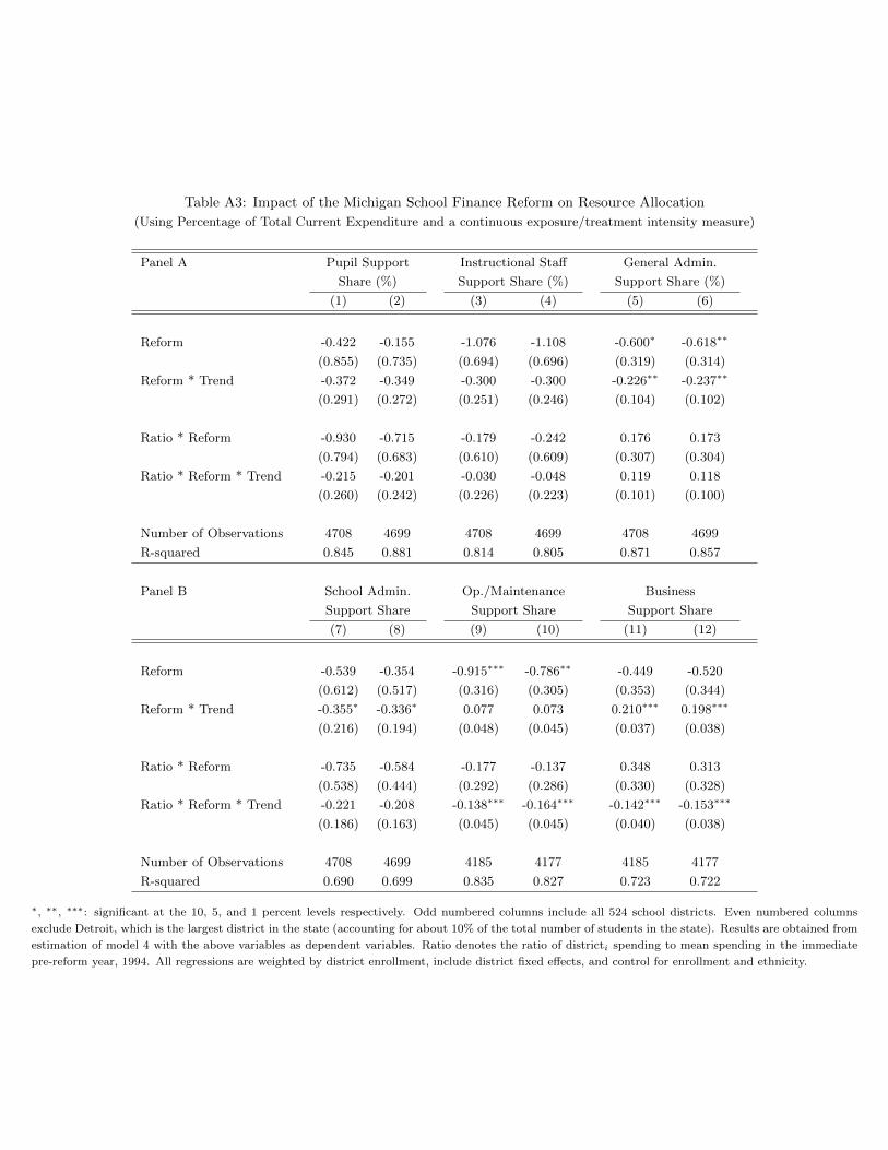
Table A3: Impact of the Michigan School Finance Reform on Resource Allocation

(Using Percentage of Total Current Expenditure and a continuous exposure/treatment intensity measure)

Panel A Pupil Support Instructional Staff General Admin.

Share (%) Support Share (%) Support Share (%)

(1) (2) (3) (4) (5) (6)

Reform -0.422 -0.155 -1.076 -1.108 -0.600∗ -0.618∗∗

(0.855) (0.735) (0.694) (0.696) (0.319) (0.314)

Reform * Trend -0.372 -0.349 -0.300 -0.300 -0.226∗∗ -0.237∗∗

(0.291) (0.272) (0.251) (0.246) (0.104) (0.102)

Ratio * Reform -0.930 -0.715 -0.179 -0.242 0.176 0.173

(0.794) (0.683) (0.610) (0.609) (0.307) (0.304)

Ratio * Reform * Trend -0.215 -0.201 -0.030 -0.048 0.119 0.118

(0.260) (0.242) (0.226) (0.223) (0.101) (0.100)

Number of Observations 4708 4699 4708 4699 4708 4699

R-squared 0.845 0.881 0.814 0.805 0.871 0.857

Panel B School Admin. Op./Maintenance Business

Support Share Support Share Support Share

(7) (8) (9) (10) (11) (12)

Reform -0.539 -0.354 -0.915∗∗∗ -0.786∗∗ -0.449 -0.520

(0.612) (0.517) (0.316) (0.305) (0.353) (0.344)

Reform * Trend -0.355∗ -0.336∗ 0.077 0.073 0.210∗∗∗ 0.198∗∗∗

(0.216) (0.194) (0.048) (0.045) (0.037) (0.038)

Ratio * Reform -0.735 -0.584 -0.177 -0.137 0.348 0.313

(0.538) (0.444) (0.292) (0.286) (0.330) (0.328)

Ratio * Reform * Trend -0.221 -0.208 -0.138∗∗∗ -0.164∗∗∗ -0.142∗∗∗ -0.153∗∗∗

(0.186) (0.163) (0.045) (0.045) (0.040) (0.038)

Number of Observations 4708 4699 4185 4177 4185 4177

R-squared 0.690 0.699 0.835 0.827 0.723 0.722

∗, ∗∗, ∗∗∗: significant at the 10, 5, and 1 percent levels respectively. Odd numbered columns include all 524 school districts. Even numbered columns

exclude Detroit, which is the largest district in the state (accounting for about 10% of the total number of students in the state). Results are obtained from

estimation of model 4 with the above variables as dependent variables. Ratio denotes the ratio of districti spending to mean spending in the immediate

pre-reform year, 1994. All regressions are weighted by district enrollment, include district fixed effects, and control for enrollment and ethnicity.

11

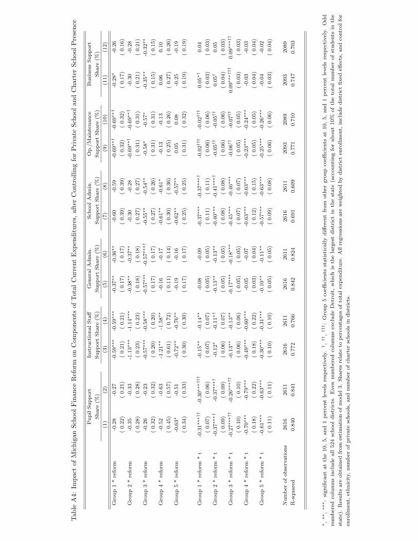
Tab

leA

4:Im

pac

tof

Mic

hig

anSch

ool

Fin

ance

Ref

orm

onC

om

pon

ents

of

Tota

lC

urr

ent

Exp

end

itu

res,

aft

erC

ontr

oll

ing

for

Pri

vate

Sch

ool

an

dC

hart

erS

chool

Pre

sen

ce

Pu

pil

Su

pp

ort

Inst

ruct

ion

al

Sta

ffG

ener

al

Ad

min

.S

chool

Ad

min

.O

p./

Main

ten

an

ceB

usi

nes

sS

up

port

Sh

are

(%)

Su

pp

ort

Sh

are

(%)

Su

pp

ort

Sh

are

(%)

Su

pp

ort

Sh

are

(%)

Su

pp

ort

Sh

are

(%)

Sh

are

(%)

(1)

(2)

(3)

(4)

(5)

(6)

(7)

(8)

(9)

(10)

(11)

(12)

Gro

up

1*

refo

rm-0

.28

-0.2

7-0

.59∗∗∗

-0.5

9∗∗∗

-0.3

7∗∗

-0.3

6∗∗

-0.6

0-0

.59

-0.6

9∗∗†

-0.6

9∗∗†

-0.2

8∗

-0.2

6

(0.2

2)

(0.2

1)

(0.2

1)

(0.2

1)

(0.1

7)

(0.1

7)

(0.3

9)

(0.3

9)

(0.3

2)

(0.3

2)

(0.1

7)

(0.1

6)

Gro

up

2*

refo

rm-0

.35

-0.3

3-1

.13∗∗∗

-1.1

4∗∗∗

-0.3

8∗∗

-0.3

7∗∗

-0.3

0-0

.28

-0.6

9∗∗†

-0.6

9∗∗†

-0.3

0-0

.28

(0.2

8)

(0.2

8)

(0.2

3)

(0.2

3)

(0.1

8)

(0.1

8)

(0.2

7)

(0.2

7)

(0.3

1)

(0.3

1)

(0.2

1)

(0.2

1)

Gro

up

3*

refo

rm-0

.26

-0.2

3-0

.57∗∗∗

-0.5

8∗∗∗

-0.5

7∗∗∗

-0.5

7∗∗∗†

-0.5

5∗∗

-0.5

4∗∗

-0.5

8∗

-0.5

7∗

-0.3

5∗∗

-0.3

2∗∗

(0.3

2)

(0.3

2)

(0.2

0)

(0.2

0)

(0.1

7)

(0.1

7)

(0.2

7)

(0.2

6)

(0.3

1)

(0.3

1)

(0.1

5)

(0.1

5)

Gro

up

4*

refo

rm-0

.52

-0.6

3-1

.21∗∗

-1.5

8∗∗

-0.1

6-0

.17

-0.6

1∗∗

-0.6

1∗

-0.1

3-0

.13

0.0

60.1

0

(0.4

5)

(0.5

7)

(0.6

1)

(0.7

2)

(0.1

1)

(0.1

4)

(0.3

0)

(0.3

6)

(0.2

5)

(0.2

6)

(0.2

7)

(0.2

6)

Gro

up

5*

refo

rm-0

.63∗

-0.5

1-0

.72∗∗

-0.7

6∗∗

-0.1

9-0

.16

-0.6

2∗∗

-0.5

7∗∗

0.0

50.0

8-0

.25

-0.1

9

(0.3

4)

(0.3

3)

(0.3

0)

(0.3

0)

(0.1

7)

(0.1

7)

(0.2

5)

(0.2

5)

(0.3

1)

(0.3

2)

(0.1

9)

(0.1

9)

Gro

up

1*

refo

rm*

t-0

.31∗∗∗††

-0.3

0∗∗∗†††

-0.1

5∗∗

-0.1

4∗∗

-0.0

8-0

.09

-0.3

7∗∗∗

-0.3

7∗∗∗†

-0.0

2†††

-0.0

2†††

0.0

5∗†

0.0

4

(0.0

7)

(0.0

6)

(0.0

7)

(0.0

7)

(0.0

5)

(0.0

5)

(0.1

1)

(0.1

1)

(0.0

6)

(0.0

6)

(0.0

3)

(0.0

3)

Gro

up

2*

refo

rm*

t-0

.37∗∗∗†

-0.3

7∗∗∗†

-0.1

2∗

-0.1

1∗†

-0.1

3∗∗

-0.1

3∗∗

-0.4

0∗∗∗

-0.4

1∗∗∗†

-0.0

5††

-0.0

5††

0.0

5†

0.0

5

(0.0

9)

(0.0

9)

(0.0

6)

(0.0

7)

(0.0

5)

(0.0

5)

(0.0

8)

(0.0

8)

(0.0

6)

(0.0

6)

(0.0

4)

(0.0

3)

Gro

up

3*

refo

rm*

t-0

.27∗∗∗††

-0.2

6∗∗∗††

-0.1

3∗∗

-0.1

3∗∗

-0.1

7∗∗∗

-0.1

8∗∗∗

-0.4

5∗∗∗

-0.4

6∗∗∗

-0.0

6††

-0.0

7††

0.0

9∗∗∗†††

0.0

9∗∗∗††

(0.1

0)

(0.1

0)

(0.0

6)

(0.0

6)

(0.0

5)

(0.0

5)

(0.0

7)

(0.0

7)

(0.0

5)

(0.0

5)

(0.0

3)

(0.0

3)

Gro

up

4*

refo

rm*

t-0

.70∗∗∗

-0.7

9∗∗∗

-0.4

9∗∗∗

-0.6

0∗∗∗

-0.0

5-0

.07

-0.6

3∗∗∗

-0.6

3∗∗∗

-0.2

3∗∗∗

-0.2

4∗∗∗

-0.0

3-0

.03

(0.1

8)

(0.2

2)

(0.1

8)

(0.2

2)

(0.0

3)

(0.0

4)

(0.1

2)

(0.1

5)

(0.0

5)

(0.0

5)

(0.0

4)

(0.0

4)

Gro

up

5*

refo

rm*

t-0

.61∗∗∗

-0.6

3∗∗∗

-0.3

0∗∗∗

-0.3

1∗∗∗

-0.1

0∗∗

-0.1

1∗∗

-0.5

7∗∗∗

-0.6

3∗∗∗

-0.2

5∗∗∗

-0.2

6∗∗∗

-0.0

4-0

.02

(0.1

1)

(0.1

1)

(0.1

0)

(0.1

0)

(0.0

5)

(0.0

5)

(0.0

9)

(0.0

8)

(0.0

6)

(0.0

6)

(0.0

3)

(0.0

4)

Nu

mb

erof

ob

serv

ati

on

s2616

2611

2616

2611

2616

2611

2616

2611

2093

2089

2093

2089

R-s

qu

are

d0.8

40

0.8

41

0.7

72

0.7

66

0.8

42

0.8

24

0.6

91

0.6

09

0.7

71

0.7

10

0.7

47

0.7

03

∗,∗∗

,∗∗∗:

sign

ifica

nt

at

the

10,

5,

an

d1

per

cent

level

sre

spec

tivel

y.† ,††

,††† :

Gro

up

5co

effici

ents

stati

stic

ally

diff

eren

tfr

om

oth

ergro

up

coeffi

cien

tsat

10,

5,

an

d1

per

cent

level

sre

spec

tivel

y.O

dd

nu

mb

ered

colu

mn

sin

clu

de

all

524

sch

ool

dis

tric

ts.

Even

nu

mb

ered

colu

mn

sex

clu

de

Det

roit

,w

hic

his

the

larg

est

dis

tric

tin

the

state

(acc

ou

nti

ng

for

ab

ou

t10%

of

the

tota

lnu

mb

erof

stu

den

tsin

the

state

).R

esu

lts

are

ob

tain

edfr

om

esti

mati

on

of

mod

el3.

Sh

are

sre

late

top

erce

nta

ges

of

tota

lex

pen

dit

ure

.A

llre

gre

ssio

ns

are

wei

ghte

dby

dis

tric

ten

rollm

ent,

incl

ud

ed

istr

ict

fixed

effec

ts,

an

dco

ntr

ol

for

enro

llm

ent,

eth

nic

ity,

nu

mb

erof

pri

vate

sch

ools

,an

dnu

mb

erof

chart

ersc

hools

ind

istr

icts

.

12

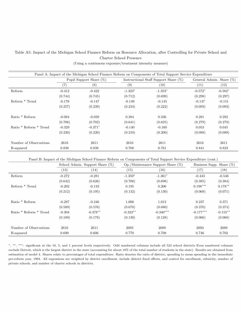
Table A5: Impact of the Michigan School Finance Reform on Resource Allocation, after Controlling for Private School and

Charter School Presence

(Using a continuous exposure/treatment intensity measure)

Panel A: Impact of the Michigan School Finance Reform on Components of Total Support Service Expenditure

Pupil Support Share (%) Instructional Staff Support Share (%) General Admin. Share (%)

(7) (8) (9) (10) (11) (12)

Reform -0.412 -0.422 -1.323∗ -1.353∗ -0.572∗ -0.582∗

(0.744) (0.745) (0.712) (0.699) (0.298) (0.297)

Reform * Trend -0.178 -0.147 -0.149 -0.145 -0.147 -0.151

(0.257) (0.239) (0.234) (0.222) (0.093) (0.093)

Ratio * Reform -0.084 -0.029 0.384 0.336 0.281 0.282

(0.706) (0.702) (0.641) (0.625) (0.279) (0.279)

Ratio * Reform * Trend -0.329 -0.371∗ -0.140 -0.160 0.053 0.045

(0.230) (0.220) (0.210) (0.200) (0.088) (0.089)

Number of Observations 2616 2611 2616 2611 2616 2611

R-squared 0.838 0.838 0.768 0.761 0.841 0.823

Panel B: Impact of the Michigan School Finance Reform on Components of Total Support Service Expenditure (cont.)

School Admin. Support Share (%) Op./Maintenance Support Share (%) Business Supp. Share (%)

(13) (14) (15) (16) (17) (18)

Reform -0.272 -0.281 -1.359∗ -1.361∗ -0.443 -0.546

(0.642) (0.626) (0.700) (0.698) (0.385) (0.384)

Reform * Trend -0.202 -0.133 0.195 0.206 0.198∗∗∗ 0.178∗∗

(0.212) (0.195) (0.132) (0.130) (0.069) (0.071)

Ratio * Reform -0.287 -0.246 1.006 1.012 0.237 0.371

(0.589) (0.576) (0.678) (0.680) (0.370) (0.374)

Ratio * Reform * Trend -0.304 -0.378∗∗ -0.323∗∗ -0.340∗∗∗ -0.177∗∗∗ -0.155∗∗

(0.189) (0.178) (0.130) (0.128) (0.066) (0.068)

Number of Observations 2616 2611 2093 2089 2093 2089

R-squared 0.690 0.606 0.770 0.708 0.746 0.702

∗, ∗∗, ∗∗∗: significant at the 10, 5, and 1 percent levels respectively. Odd numbered columns include all 524 school districts Even numbered columns

exclude Detroit, which is the largest district in the state (accounting for about 10% of the total number of students in the state). Results are obtained from

estimation of model 4. Shares relate to percentages of total expenditure. Ratio denotes the ratio of districti spending to mean spending in the immediate

pre-reform year, 1994. All regressions are weighted by district enrollment, include district fixed effects, and control for enrollment, ethnicity, number of

private schools, and number of charter schools in districts.

13

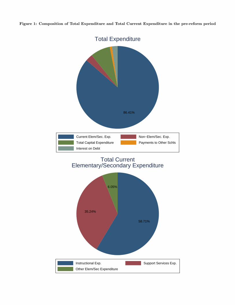
Figure 1: Composition of Total Expenditure and Total Current Expenditure in the pre-reform period

86.41%

Current Elem/Sec. Exp. Non−Elem/Sec. Exp.

Total Capital Expenditure Payments to Other Schls

Interest on Debt

Total Expenditure

58.71%

35.24%

6.05%

Instructional Exp. Support Services Exp.

Other Elem/Sec Expenditure

Total CurrentElementary/Secondary Expenditure

1

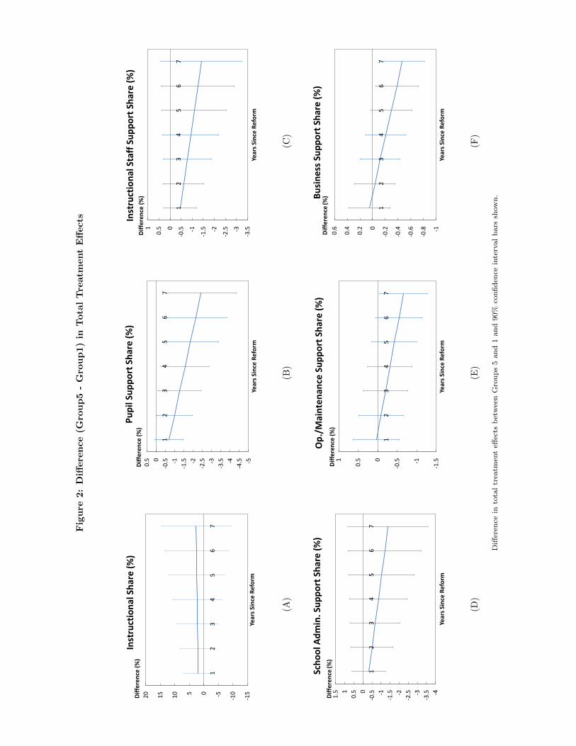
Fig

ure

2:

Diff

ere

nce

(Gro

up

5-

Gro

up

1)

inT

ota

lT

reatm

ent

Eff

ects

-15

-10-505101520

12

34

56

7

Year

s Sin

ce R

efor

m

Inst

ruct

iona

l Sha

re (%

) Di

ffere

nce

(%)

-5-4

.5-4-3

.5-3-2

.5-2-1

.5-1-0

.500.

5

12

34

56

7

Year

s Sin

ce R

efor

m

Pupi

l Sup

port

Sha

re (%

) Di

ffere

nce

(%)

-3.5-3

-2.5-2

-1.5-1

-0.50

0.51

12

34

56

7

Year

s Sin

ce R

efor

m

Diffe

renc

e (%

) In

stru

ctio

nal S

taff

Sup

port

Sha

re (%

)

(A)

(B)

(C)

-4-3

.5-3-2

.5-2-1

.5-1-0

.500.

511.

5

12

34

56

7

Year

s Sin

ce R

efor

m

Scho

ol A

dmin

. Sup

port

Sha

re (%

) Di

ffere

nce

(%)

-1.5-1

-0.50

0.51

12

34

56

7

Year

s Sin

ce R

efor

m

Diffe

renc

e (%

)

Op.

/Mai

nten

ance

Sup

port

Sha

re (%

)

-1

-0.8

-0.6

-0.4

-0.20

0.2

0.4

0.6

12

34

56

7

Year

s Sin

ce R

efor

m

Busi

ness

Sup

port

Sha

re (%

) Di

ffere

nce

(%)

(D)

(E)

(F)

Diff

eren

cein

tota

ltr

eatm

ent

effec

tsb

etw

een

Gro

up

s5

an

d1

an

d90%

con

fid

ence

inte

rval

bars

show

n.

2

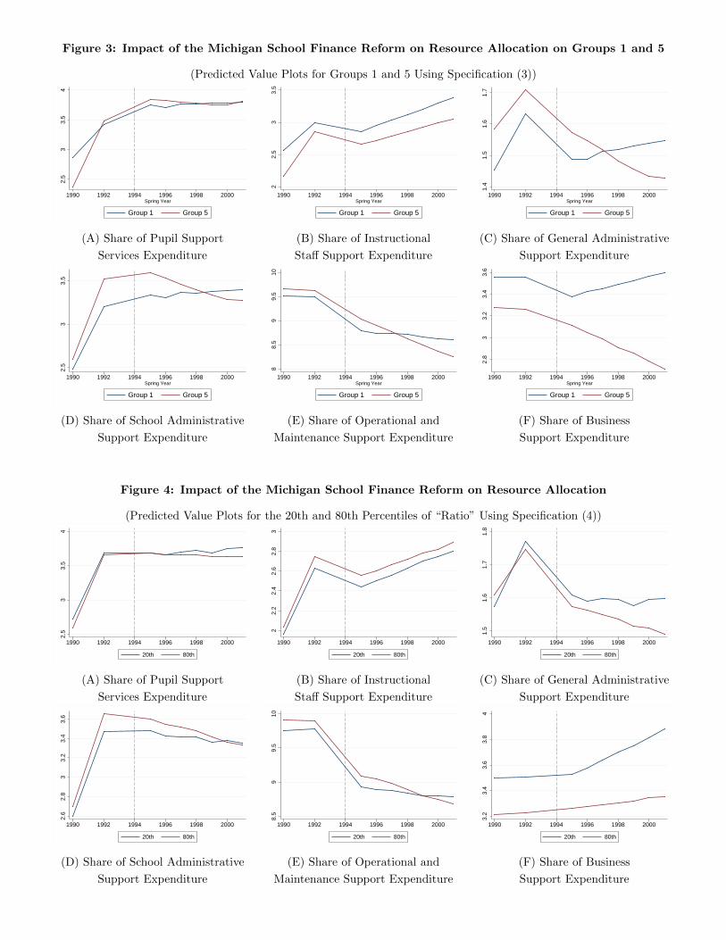
Figure 3: Impact of the Michigan School Finance Reform on Resource Allocation on Groups 1 and 5

(Predicted Value Plots for Groups 1 and 5 Using Specification (3))2.

53

3.5

4

1990 1992 1994 1996 1998 2000Spring Year

Group 1 Group 5

22.

53

3.5

1990 1992 1994 1996 1998 2000Spring Year

Group 1 Group 5

1.4

1.5

1.6

1.7

1990 1992 1994 1996 1998 2000Spring Year

Group 1 Group 5

(A) Share of Pupil Support (B) Share of Instructional (C) Share of General Administrative

Services Expenditure Staff Support Expenditure Support Expenditure

2.5

33.

5

1990 1992 1994 1996 1998 2000Spring Year

Group 1 Group 5

88.

59

9.5

10

1990 1992 1994 1996 1998 2000Spring Year

Group 1 Group 5

2.8

33.

23.

43.

6

1990 1992 1994 1996 1998 2000Spring Year

Group 1 Group 5

(D) Share of School Administrative (E) Share of Operational and (F) Share of Business

Support Expenditure Maintenance Support Expenditure Support Expenditure

Figure 4: Impact of the Michigan School Finance Reform on Resource Allocation

(Predicted Value Plots for the 20th and 80th Percentiles of “Ratio” Using Specification (4))

2.5

33.

54

1990 1992 1994 1996 1998 2000

20th 80th

22.

22.

42.

62.

83

1990 1992 1994 1996 1998 2000

20th 80th

1.5

1.6

1.7

1.8

1990 1992 1994 1996 1998 2000

20th 80th

(A) Share of Pupil Support (B) Share of Instructional (C) Share of General Administrative

Services Expenditure Staff Support Expenditure Support Expenditure

2.6

2.8

33.

23.

43.

6

1990 1992 1994 1996 1998 2000

20th 80th

8.5

99.

510

1990 1992 1994 1996 1998 2000

20th 80th

3.2

3.4

3.6

3.8

4

1990 1992 1994 1996 1998 2000

20th 80th

(D) Share of School Administrative (E) Share of Operational and (F) Share of Business

Support Expenditure Maintenance Support Expenditure Support Expenditure

3