This article was downloaded by: [Korea University]On: 02 February 2014, At: 22:07Publisher: Taylor & FrancisInforma Ltd Registered in England and Wales Registered Number: 1072954 Registered office: Mortimer House,37-41 Mortimer Street, London W1T 3JH, UK

International Journal of Computational Fluid DynamicsPublication details, including instructions for authors and subscription information:http://www.tandfonline.com/loi/gcfd20

Effect of confinement on droplet deformation in shearflowHaobo Huaa, Yibao Lib, Jaemin Shina, Ha-kyu Songa & Junseok Kima

a Department of Mathematics, Korea University, Seoul 136-713, Republic of Koreab Department of Computational Science and Engineering, Yonsei University, Seoul 120-749,Republic of KoreaPublished online: 12 Nov 2013.

To cite this article: Haobo Hua, Yibao Li, Jaemin Shin, Ha-kyu Song & Junseok Kim (2013) Effect of confinement ondroplet deformation in shear flow, International Journal of Computational Fluid Dynamics, 27:8-10, 317-331, DOI:10.1080/10618562.2013.857406

To link to this article: http://dx.doi.org/10.1080/10618562.2013.857406

PLEASE SCROLL DOWN FOR ARTICLE

Taylor & Francis makes every effort to ensure the accuracy of all the information (the “Content”) containedin the publications on our platform. However, Taylor & Francis, our agents, and our licensors make norepresentations or warranties whatsoever as to the accuracy, completeness, or suitability for any purpose of theContent. Any opinions and views expressed in this publication are the opinions and views of the authors, andare not the views of or endorsed by Taylor & Francis. The accuracy of the Content should not be relied upon andshould be independently verified with primary sources of information. Taylor and Francis shall not be liable forany losses, actions, claims, proceedings, demands, costs, expenses, damages, and other liabilities whatsoeveror howsoever caused arising directly or indirectly in connection with, in relation to or arising out of the use ofthe Content.

This article may be used for research, teaching, and private study purposes. Any substantial or systematicreproduction, redistribution, reselling, loan, sub-licensing, systematic supply, or distribution in anyform to anyone is expressly forbidden. Terms & Conditions of access and use can be found at http://www.tandfonline.com/page/terms-and-conditions

International Journal of Computational Fluid Dynamics, 2013Vol. 27, Nos. 8–10, 317–331, http://dx.doi.org/10.1080/10618562.2013.857406

RESEARCH ARTICLE

Effect of confinement on droplet deformation in shear flow

Haobo Huaa, Yibao Lib, Jaemin Shina, Ha-kyu Songa and Junseok Kima,∗

aDepartment of Mathematics, Korea University, Seoul 136-713, Republic of Korea; bDepartment of Computational Science andEngineering, Yonsei University, Seoul 120-749, Republic of Korea

(Received 21 September 2012; accepted 14 October 2013)

The dynamics of a single droplet under shear flow between two parallel plates is investigated by using the immersed boundarymethod. The immersed boundary method is appropriate for simulating the drop-ambient fluid interface. We apply a volume-conserving method using the normal vector of the surface to prevent mass loss of the droplet. In addition, we present asurface remeshing algorithm to cope with the distortion of droplet interface points caused by the shear flow. This meshquality improvement in conjunction with the volume-conserving algorithm is particularly essential and critical for long timeevolutions. We study the effect of wall confinement on the droplet dynamics. Numerical simulations show good agreementwith previous experimental results and theoretical models.

Keywords: wall effect; immersed boundary method; shear flow; volume conserving; remeshing; droplet deformation

1. Introduction

Deformation and breakup of droplets play an important rolein the morphological development of blends (Tucker III andMoldenaers 2002) as can be seen from their applications inindustry and natural processes such as in emulsions, ink-jetprinters, oil recovery and biological cell systems. Let usconsider two immiscible fluids, with a droplet of one fluidsurrounded by another ambient fluid with a Newtonian vis-cosity η and interfacial tension coefficient σ . There aretwo main parameters that determine the deformation andbreakup behaviour of the droplet component: the capillarynumber Ca and the viscosity ratio λ. The capillary numberis defined as Ca = ηmRγ /σ , where ηm, R and γ denote theviscosity of the ambient fluid, the radius of the undeformeddroplet, and the shear rate, respectively. The capillary num-ber expresses the ratio between viscous stresses that distortthe droplet shape and interfacial stresses that restore thedroplet shape. The viscosity ratio is defined as the ratio ofthe droplet viscosity to the ambient fluid viscosity: λ =ηd/ηm, where ηd is the droplet viscosity.

The degree of confinement or confinement ratio is de-fined as the ratio of the droplet diameter to the distance be-tween two parallel plates. After the pioneering research onthe dynamics of small droplets immersed in another fluid byTaylor (1932, 1934), most investigations have concentratedon the unconfined droplet deformation and breakup ex-perimentally and theoretically (Chaffey and Brenner 1967;Rallison 1984). Several reviews are available in the lit-erature (Stone 1994; Tucker III and Moldenaers 2002;Cristini and Renardy 2006). For the numerical simulation

∗Corresponding author. Email: cfdkim@korea.ac.kr

of the droplet dynamics, a number of different methodolo-gies have been developed, including the volume-of-fluid(Gueyffier et al. 1999; Renardy and Cristini 2001; Renardy2007), boundary-integral (Cristini et al. 2003; Janssen andAnderson 2007; Vananroye et al. 2008), phase-field (Yueet al. 2004; Kim 2005; Yue et al. 2006; Ceniceros, Nos,and Roma 2010), level set (Pillapakkam and Singh 2001;Xu et al. 2006; Ardekani, Dabiri, and Rangel 2009), andimmersed boundary methods (IBM; Sheth and Pozrikidis1995).

The desired droplet-size distribution in multiphase sys-tems, which is important in industrial processes, has beenstudied (Thorsen et al. 2001; Tice, Lyon, and Ismagilov2004; Garstecki, Stone, and Whitesides 2005). In thesemultiphase systems, the droplet diameter is typically of theorder of the parallel plate height; therefore, wall effects playan important role on droplet deformation. Many experimen-tal and numerical investigations on the behaviour of a sin-gle droplet especially under confined shear flow have beenperformed (Sibillo et al. 2006; Vananroye, Van Puyvelde,and Moldenaers 2006a, 2006b; Griggs, Zinchenko, andDavis 2007; Janssen and Anderson 2007; Renardy 2007;Vananroye, Van Puyvelde, and Moldenaers 2007;Cardinaels et al. 2011).

Janssen and Anderson (2007) studied the evolution ofthe shape of a single droplet placed between two paral-lel plates using the boundary-integral method. The authorsinvestigated the influence of the capillary number and con-finement ratio on droplet deformation. Vananroye et al.(2008) also used the boundary-integral method to compare

C© 2013 Taylor & Francis

Dow

nloa

ded

by [

Kor

ea U

nive

rsity

] at

22:

07 0

2 Fe

brua

ry 2

014

318 H. Hua et al.

the experimental and numerical results. They predicted anincrease in droplet deformation and greater orientation tothe flow direction with the increase of the degree of confine-ment. Cardinaels et al. (2011) numerically investigated theeffect of confinement on the droplet dynamics after startupof shear flow for systems with one viscoelastic componentusing the volume-of-fluid method. They found that con-finement substantially increases the elongation rate in andaround the droplet. Shapira and Haber (1988) gave a the-oretical prediction of single droplet deformation at steadystate under confined shear flow. Recently, Minale (2008)developed a phenomenological model, which is forced torecover the small deformation limits of Shapira and Haber(1990), successfully matching the experimental data avail-able in the literature. See Minale (2010) for a review onthe theoretical models for the deformation of a single ellip-soidal droplet.

In this paper, we focus on the investigation of the dy-namics of droplet deformation with wall confinement. Weuse the IBM to study droplet dynamics. In general, the IBMdoes not guarantee the conservation of volume. Therefore,we apply the area-preserving method (Li et al. 2012) andvolume-conserving method (Li et al. 2013) to overcome thelack of conservation in the IBM. In previous work (Li et al.2013), however, there has been a limitation for the long-timeevolution and large deformation because of mesh distortion.The goal of this paper is to incorporate a surface remeshingalgorithm into the recently developed volume-conservingIBM (Li et al. 2013) for two-phase fluid flow. In this work,we apply the volume mesh generator DistMesh developedby Persson and Strang (2004) and Persson (2006) to remeshthe distorted surface mesh.

The rest of the paper is organised as follows. In Section2, we state the problem of droplet deformation in shear flowand introduce the mathematical formulations. In Section 3,we describe the numerical implementation of the remeshingalgorithm, construction of the signed distance function andIBM. Sections 4 and 5 present numerical results in twoand three dimensions, respectively. Finally, conclusions aredrawn in Section 6.

2. Problem statement and governing equations

We consider the dynamical motion of a single droplet in anambient fluid between two parallel plates as schematicallydepicted in Figure 1. The velocity vector field is generatedby the boundary condition for u = (±γ H, 0, 0) at z = ±H,where H is the wall height and γ is the shear rate. For thex- and y-directions, we use a periodic boundary conditionfor the velocity u. For the pressure variable, we impose aperiodic boundary condition for the x- and y-directions anda zero-Neumann boundary condition for the z-direction.To measure the magnitude of the deformation, we use theTaylor deformation number defined by D = (L − B)/(L +B), where L and B are, respectively, the major and minor

Figure 1. Schematic illustration for a liquid droplet (Fluid 2) inan ambient fluid (Fluid 1) under shear flow.

drop semiaxes in the x–z plane. W is another semiaxis in thex–y plane. The orientation angle θ is defined as the anglebetween the L-axis and the velocity direction.

The mathematical model is based on the IBM developedby Peskin (1977). Let the fluid velocity u(x, t) = (u(x, t),v(x, t), w(x, t)) be defined on the fixed Cartesian coordinatex = (x, y, z) at time t. We denote X(t) as the Lagrangianvariable for the immersed boundary. The Lagrangian vari-able X(t) separates the domain into two regions occupied bytwo distinct fluids. The fluid flow is computed in the wholedomain and then X(t) is advected by the interpolated fluidvelocity from u(x, t). The fluid interacts with the boundaryvia singular forces exerted by the boundary. This surfacetension force is spread to the surrounding Eulerian variablex using a delta function. We suppose that the density andviscosity are both constant. The dimensionless equations ofmotion for the system are as follows:

∂u(x, t)

∂t+ u(x, t) · ∇u(x, t)

= −∇p(x, t) + 1

Re�u(x, t) + 1

Wef(x, t), (1)

∇ · u(x, t) = 0, (2)

f(x, t) =∫

F(X(t))δ(x − X(t))ds, (3)

U(X(t)) =∫

�

u(x, t)δ(x − X(t))dx, (4)

dX(t)

dt= U(X(t)). (5)

Here, � is the domain and is the interface betweenthe two fluids. The Reynolds number in Equation (1) isdefined as Re = ρmR2γ /ηm, where ρm is the density of theambient fluid. Then, the Weber number can be defined asWe = Re · Ca. The fluid velocity u(x, t), pressure p(x, t), andsingular surface tension force f(x, t) are Eulerian variablesin a Cartesian domain � ∈ R

d (d = 2 or 3). The boundaryforce density F(X(t)) and boundary velocity U(X(t)) are

Dow

nloa

ded

by [

Kor

ea U

nive

rsity

] at

22:

07 0

2 Fe

brua

ry 2

014

International Journal of Computational Fluid Dynamics 319

Figure 2. (a) Velocities defined at cell interfaces and pressure defined at the cell centres in three dimensions. (b) Illustration of Eulerianpoints x and Lagrangian points X(t). (a) MAC mesh. (b) Immersed boundary.

Lagrangian variables. F(X(t)) is defined as

F(X(t)) = κ(X(t))n(X(t)), (6)

where κ is the mean curvature and n is the unit outwardnormal vector. δ(x − X(t)) is the Dirac delta function, whichis defined by the product of one-dimensional Dirac deltafunctions, i.e. δ(x) = δ(x)δ(y) and δ(x) = δ(x)δ(y)δ(z) intwo and three dimensions, respectively.

3. Numerical implementation

In this section, we briefly describe the DistMesh algorithmand IBM in three dimensions. During the simulation ofdroplet deformation in shear flow by the IBM, the distribu-tion of surface mesh could be seriously distorted. In a longtime simulation, this distorted mesh distribution could leadto an inaccurate calculation of surface curvature. Eventu-ally, the droplet shape will not well maintained. The rest ofthis section is devoted to explaining the algorithm for regen-erating the surface mesh in conjunction with the volume-conserving IBM.

3.1. Discretisation

We discretise the domain � = (a, b) × (c, d) × (e, f) inthree-dimensional space. Two-dimensional discretisation isanalogously defined. Let a computational domain be par-titioned into a uniform mesh with a space step size h in aCartesian geometry. The center of each cell is located atxijk = (xi, yj, zk), where xi = a + (i − 0.5)h, yj = c +(j − 0.5)h, and zk = e + (k − 0.5)h, for i = 1, . . . , Nx, j =1, . . . , Ny and k = 1, . . . , Nz. Here, Nx, Ny and Nz are thenumbers of cells in the x-, y-, and z-directions, respectively.

Let unijk be an approximation of u(xi, yj, zk, tn), where tn =

n�t and �t is the time step size.We use a staggered marker-and-cell mesh, in which

pressure is stored at cell centres and velocities are stored atcell interfaces (Harlow and Welch 1965). Velocity compo-nents u, v, and w are defined at the x-, y-, and z-directionalface centres, respectively (see Figure 2(a)). We use a set ofM Lagrangian points Xn

l = (Xnl , Y

nl , Zn

l ) for l = 1, . . . , Mto discretise the immersed boundary. There are MT trian-gles Tris = (Xl, Xm, Xq) for s = 1, . . . , MT with the threevertices Xl, Xm and Xq for each triangle being orderedcounterclockwise (see Figure 2(b)).

3.2. DistMesh algorithm for the surface mesh

To generate the triangular surface mesh using the implicitrepresentation of the surface, we use the DistMesh algo-rithm (Persson and Strang 2004; Persson 2006). Let us takea two-dimensional example to illustrate the basic idea ofthe algorithm. Let the interface of two fluids be implicitlyrepresented as the zero-level set of an implicit function.For example, the function φ(x, y) =

√x2 + y2 − 1 implic-

itly represents the unit circle by the zero level set φ = 0,which is shown by the dashed curve in Figure 3. The mainprocedure for generating the triangular surface mesh is asfollows (where, to simplify the explanation, we denote thenode points at Step 1 by Xn, 1. Xn, 2 and Xn, 3 are defined ina similar manner):

Step 1. Assign the repulsive force depending on the lengthof the edge of each triangle and calculate the net force atnode points Xn, 1 (see Figure 3(a)).

Step 2. According to the net force, move node points Xn, 1

to Xn, 2 (see Figure 3(b)).

Dow

nloa

ded

by [

Kor

ea U

nive

rsity

] at

22:

07 0

2 Fe

brua

ry 2

014

320 H. Hua et al.

Figure 3. Surface mesh generation: (a) net force vectors, (b) triangulation after moving points, (c) projection to the interface, and (d)final triangulation. (a) Xn, 1. (b) Xn, 2. (c) Xn, 3. (d) Final.

Step 3. To get Xn, 3, project node points Xn, 2 to the zero-level contour with respect to the normal direction |∇φ| (seeFigure 3(c)).

We repeat Steps 1–3 until the mesh uniformity is sat-isfactory, i.e. until the movements of node points are lessthan a given tolerance (see Figure 3(d)). The projection stepshould be applied because points slightly deviate from thezero-level set by Step 2. To project the point Xn,2

l to thesurface φ = 0 at the Step 3, we use the first-order approxi-mation

Xn,3l = Xn,2

l − φ(Xn,2

l

) ∇φ(Xn,2

l

)∣∣∇φ

(Xn,2

l

)∣∣2. (7)

In the three-dimensional case, the above algorithm isnot sufficient for the moving points to satisfy the meshuniformity. To obtain a high-quality triangulation, we up-date the connectivity to maintain good triangulation of thenodes during the iterations. We only update the bad tri-angles by changing the local connectivity. In the flipping

algorithm, we sweep all elements and consider flipping theedge between neighbouring triangles. For example, the tri-angles Tris1 = (Xa, Xb, Xd ) and Tris2 = (Xa, Xc, Xb) inFigure 4(a) change to Tris1 = (Xa, Xc, Xd ) and Tris2 =(Xc, Xb, Xd ) in Figure 4(b).

3.3. Signed distance function

We use the surface mesh, which is the immersed bound-ary surface, to construct a signed distance function. Theinterface between two fluids is implicitly defined by usingthe signed distance function. Let us take a two-dimensionalexample to illustrate the basic idea of the method. We take20 uniformly distributed points for a circle of radius 0.25on the computational domain (0, 1) × (0, 1) discretised bya 32 × 32 mesh. Each element distributes the distance andorientation from itself to nearby points (see Figure 5(a)).At the point that receives data, we compare the receivingand existing distances, then choose the smaller one and itsorientation. After all elements distribute data, we have theshortest distance and its orientation to the surface at a set

Figure 4. Schematic illustration of the flipping algorithm.

Dow

nloa

ded

by [

Kor

ea U

nive

rsity

] at

22:

07 0

2 Fe

brua

ry 2

014

International Journal of Computational Fluid Dynamics 321

Figure 5. Schematic illustration for constructing a signed distance function by using the surface elements. (a) Nearby points. (b) Signeddistance function. (c) Contour.

of points within a band around the evaluated surface (seeFigure 5(b)). Figure 5(c) shows the node points and zerocontour. The more surface elements there are, the smootherthe zero contour of a signed distance function is.

We extend the above algorithm to the three-dimensionalcase. Suppose one triangular mesh Tris = (Xl, Xm, Xq) onthe surface distributes the distance and its orientation to thepoint xijk, which is on the Cartesian grid. Now, we describethe formula to find the shortest distance from the point xijk tothe triangle and denote the point on the triangle as E wherethe distance is minimum. To simplify the explanation, wedefine four vectors as follows: p = −−−→

xijkE, q = −−−−→xijkXm, v1 =−−−→XmXl and v2 = −−−→XmXq . Then, we can describe the vector onthe triangular mesh by the parameters α and β as follows:p − q = αv1 + βv2, where 0 ≤ α + β ≤ 1, α ≥ 0, andβ ≥ 0. Finding the minimum distance from the triangularmesh to point E is equivalent to finding a minimum valueof ‖p‖2 (see Figure 6).

We define the distance function between point E andthe triangular mesh by

f (α, β) = ‖p‖2 = ‖v1‖2α2 + ‖v2‖2β2 + ‖q‖2

+ 2vT1 v2αβ + 2vT

1 qα + 2vT2 qβ. (8)

There are seven potential candidates to be minimum: acritical point, three node points and three boundary points.Note that the function f is a convex function for all α andβ since fααfββ − f 2

αβ > 0. Therefore, if there is a criticalpoint in the shaded region, f has a minimum value on it.

3.4. Immersed boundary method

At the nth time step, we have a velocity field un, whichis divergence-free, and a surface tension function fn

ijk

calculated by the boundary configuration Xn. An outline

Figure 6. Schematic illustration of the construction of the signed distance function in three dimensions.

Dow

nloa

ded

by [

Kor

ea U

nive

rsity

] at

22:

07 0

2 Fe

brua

ry 2

014

322 H. Hua et al.

of the main procedure in one time step containing the vol-ume correction and remeshing algorithms is as follows:

Step 1. Surface tension force

Evaluate the boundary force density Fnl from the boundary

configuration Xn,

Fnl = κn

l nnl , (9)

for l = 1, . . . , M, where κnl is the mean curvature and nn

l

is the normal vector. We then calculate the surface tensionforce fn

ijk .

fnijk =

M∑l=1

Fnl δh

(xijk − Xn

l

)�Al , (10)

for i = 1, . . . , Nx, j = 1, . . . , Ny and k = 1, . . . , Nz, where δh

is a smoothed Dirac delta function (Peskin and McQueen1995) and �Al is a surface area element. The reader couldrefer to Li et al. (2013) for details of calculations of curva-ture and normal vector.

Step 2. Calculation of momentum equation

The Navier–Stokes Equations (1) and (2) are solved byusing a projection method. First, we solve an advection–diffusion equation including surface tension fn in the ab-sence of the pressure, resulting an intermediate velocityu,

u − un

�t+ un · ∇dun = 1

Re�un + 1

Wefn (11)

where ∇d and �d denote the centred difference approxima-tions for the gradient and Laplacian operators, respectively.Second, we solve the following equation for the advancedpressure field

un+1 − u

�t= −∇dp

n+1. (12)

The pressure pn + 1 is obtained from the fact that the veloc-ity field is divergence-free at (n + 1)th time step

�dpn+1 = 1

�t∇d · u, (13)

where ∇d· denotes the discrete divergence operator. Theresulting system of Equation (13) is solved using a multigridmethod (Trottenberg, Oosterlee, and Schuller 2001). Thevelocity field un + 1 is then computed by

un+1 = u − �t∇dpn+1. (14)

Step 3. Updating the interface variables

The new immersed boundary velocity Un+1l and

position Xn+1l

Un+1l =

Nx∑i=1

Ny∑j=1

Nz∑k=1

un+1ijk δh

(xijk − Xn

l

)h3, (15)

Xn+1l = Xn

l + �tUn+1l , l = 1, . . . , M. (16)

These Steps 1–3 complete the procedure for calculating thefluid velocity un + 1 and boundary position Xn + 1.

We then apply the volume-conserving algorithm (Liet al. 2013) to Xn + 1 for keeping the initial volume. In ad-dition, after several time steps, we construct the signed dis-tance function using the immersed boundary surface mesh(Section 3.3) and apply the distance function to the remesh-ing algorithm (Section 3.2) to maintain the mesh uniformityand quality.

4. Numerical experiments in two dimensions

In this section, we perform numerical experiments in twodimensions. The convergence tests and the comparison withprevious results are performed to verify our algorithm. Wethen investigate the effects of the domain size and initialshape on the droplet evolution. In addition, the steady-state droplet shapes are investigated in details under variousconditions.

4.1. Convergence test

We calculate the dimensionless axes L/R and B/R to de-scribe the deformation of the drop (Minale 2008). A dropwith radius R = 0.5 is located in the centre of the compu-tational domain � = (−1, 1) × (−1, 1). Other parametersare Re = 10, Ca = 0.2 and γ = 1. Figure 7 shows theevolutions of the dimensionless axes and orientation anglewith increasing mesh size: 32 × 32, 64 × 64, 128 × 128 and256 × 256. Here, we use the time step �t = 0.1h2 depend-ing on the space step size h. With the increase of mesh size,the results become convergent.

We next investigate the effect of the number of markerpoints on the results. The results are calculated on the do-main (−1, 1) × (−1, 1), where the space step size h = 1/32.The initial interface is a circle with radius R = 0.5. Let Mbe the number of marker points, and the marker points areevenly distributed on the interface 2πR at the initial state.Figure 8 shows droplet shapes with different numbers ofmarker points in steady state. The increasing number ofmarker points improves the accuracy of interface presenta-tion, but there is a little difference. Thus, in the followingtwo-dimensional simulations, we will use a moderate valueof M defined as the nearest integer number of 2πRm/h,where m is a integer. A Lagrangian mesh size then approx-imates to h/m. We will use a modest value of m = 4.

Dow

nloa

ded

by [

Kor

ea U

nive

rsity

] at

22:

07 0

2 Fe

brua

ry 2

014

International Journal of Computational Fluid Dynamics 323

Figure 7. Convergence of (a) dimensionless axes and (b) orientation angle with different mesh sizes.

4.2. Comparison with previous result

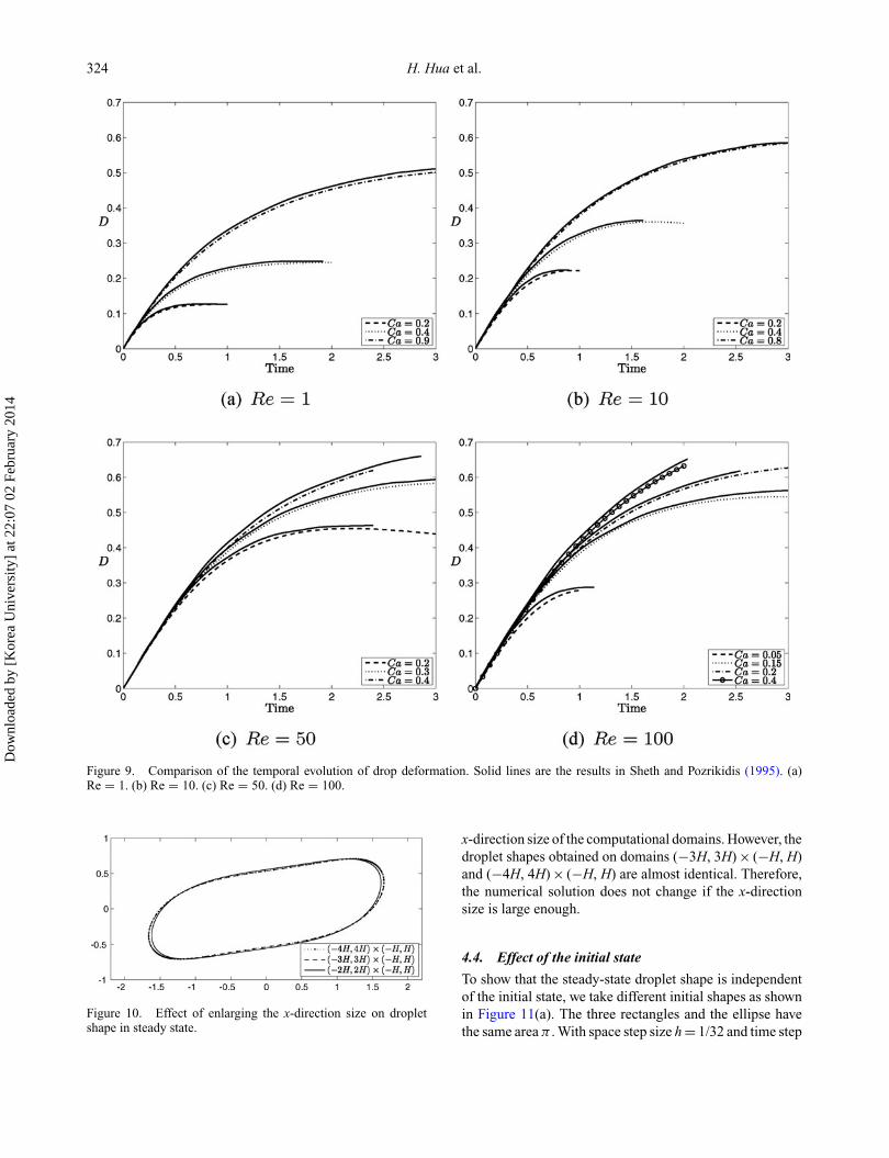
We compare our results with previous results (Sheth andPozrikidis 1995). In Sheth and Pozrikidis (1995), a 24 × 24mesh grid is used on the domain (−1, 1) × (−1, 1). Forcomparison, we choose a 32 × 32 mesh with the same pa-rameters. Figure 9 shows the deformation number D asa function of time with different Reynolds and capillarynumbers. Our results agree well with those of the previousstudies.

4.3. Effect of the domain size

We perform simulations with different domain sizes,(−2H, 2H) × (−H, H), (−3H, 3H) × (−H, H) and (−4H,4H) × (−H, H) where the wall height H = 1.25R and thedroplet radius R = 1. The parameters Ca = 0.25, Re = 1γ = 1, and h = H/128 are used. The initial interface is a cir-cle with radius R = 0.5. Figure 10 shows the drop shapes insteady state with a time step size �t = 0.1h2. Because of theperiodic boundary condition, the solutions depend on the

Figure 8. (a) Droplet shape at steady state with different numbers of marker points. (b) Expanded view for different marker points.

Dow

nloa

ded

by [

Kor

ea U

nive

rsity

] at

22:

07 0

2 Fe

brua

ry 2

014

324 H. Hua et al.

Figure 9. Comparison of the temporal evolution of drop deformation. Solid lines are the results in Sheth and Pozrikidis (1995). (a)Re = 1. (b) Re = 10. (c) Re = 50. (d) Re = 100.

Figure 10. Effect of enlarging the x-direction size on dropletshape in steady state.

x-direction size of the computational domains. However, thedroplet shapes obtained on domains (−3H, 3H) × (−H, H)and (−4H, 4H) × (−H, H) are almost identical. Therefore,the numerical solution does not change if the x-directionsize is large enough.

4.4. Effect of the initial state

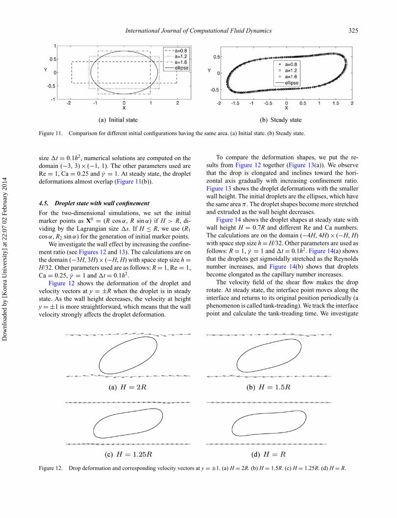
To show that the steady-state droplet shape is independentof the initial state, we take different initial shapes as shownin Figure 11(a). The three rectangles and the ellipse havethe same area π . With space step size h = 1/32 and time step

Dow

nloa

ded

by [

Kor

ea U

nive

rsity

] at

22:

07 0

2 Fe

brua

ry 2

014

International Journal of Computational Fluid Dynamics 325

Figure 11. Comparison for different initial configurations having the same area. (a) Initial state. (b) Steady state.

size �t = 0.1h2, numerical solutions are computed on thedomain (−3, 3) × (−1, 1). The other parameters used areRe = 1, Ca = 0.25 and γ = 1. At steady state, the dropletdeformations almost overlap (Figure 11(b)).

4.5. Droplet state with wall confinement

For the two-dimensional simulations, we set the initialmarker points as X0 = (R cos α, R sin α) if H > R, di-viding by the Lagrangian size �s. If H ≤ R, we use (R1

cos α, R2 sin α) for the generation of initial marker points.We investigate the wall effect by increasing the confine-

ment ratio (see Figures 12 and 13). The calculations are onthe domain (−3H, 3H) × (−H, H) with space step size h =H/32. Other parameters used are as follows: R = 1, Re = 1,Ca = 0.25, γ = 1 and �t = 0.1h2.

Figure 12 shows the deformation of the droplet andvelocity vectors at y = ±R when the droplet is in steadystate. As the wall height decreases, the velocity at heighty = ±1 is more straightforward, which means that the wallvelocity strongly affects the droplet deformation.

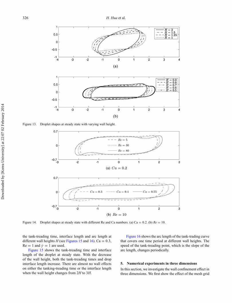
To compare the deformation shapes, we put the re-sults from Figure 12 together (Figure 13(a)). We observethat the drop is elongated and inclines toward the hori-zontal axis gradually with increasing confinement ratio.Figure 13 shows the droplet deformations with the smallerwall height. The initial droplets are the ellipses, which havethe same area π . The droplet shapes become more stretchedand extruded as the wall height decreases.

Figure 14 shows the droplet shapes at steady state withwall height H = 0.7R and different Re and Ca numbers.The calculations are on the domain (−4H, 4H) × (−H, H)with space step size h = H/32. Other parameters are used asfollows: R = 1, γ = 1 and �t = 0.1h2. Figure 14(a) showsthat the droplets get sigmoidally stretched as the Reynoldsnumber increases, and Figure 14(b) shows that dropletsbecome elongated as the capillary number increases.

The velocity field of the shear flow makes the droprotate. At steady state, the interface point moves along theinterface and returns to its original position periodically (aphenomenon is called tank-treading). We track the interfacepoint and calculate the tank-treading time. We investigate

Figure 12. Drop deformation and corresponding velocity vectors at y = ±1. (a) H = 2R. (b) H = 1.5R. (c) H = 1.25R. (d) H = R.

Dow

nloa

ded

by [

Kor

ea U

nive

rsity

] at

22:

07 0

2 Fe

brua

ry 2

014

326 H. Hua et al.

Figure 13. Droplet shapes at steady state with varying wall height.

Figure 14. Droplet shapes at steady state with different Re and Ca numbers. (a) Ca = 0.2. (b) Re = 10.

the tank-treading time, interface length and arc length atdifferent wall heights H (see Figures 15 and 16). Ca = 0.3,Re = 1 and γ = 1 are used.

Figure 15 shows the tank-treading time and interfacelength of the droplet at steady state. With the decreaseof the wall height, both the tank-treading times and dropinterface length increase. There are almost no wall effectson either the tanking-treading time or the interface lengthwhen the wall height changes from 2H to 3H.

Figure 16 shows the arc length of the tank-trading curvethat covers one time period at different wall heights. Thespeed of the tank-treading point, which is the slope of thearc length, changes periodically.

5. Numerical experiments in three dimensions

In this section, we investigate the wall confinement effect inthree dimensions. We first show the effect of the mesh grid

Dow

nloa

ded

by [

Kor

ea U

nive

rsity

] at

22:

07 0

2 Fe

brua

ry 2

014

International Journal of Computational Fluid Dynamics 327

Figure 15. (a) Tank-treading time and (b) interface length of the droplet versus wall height in steady state. (a) Tank-treading time. (b)Interface length.

size and the number of interface points. A comparison ofwith and without remeshing algorithm is performed to il-lustrate the necessity of using the remeshing procedure. Wethen study the droplet state in the confined wall by com-paring with the experimental data and theoretical values.Finally, we show the effect of Re and Ca numbers on thedroplet shape for the more confined wall height.

For the three-dimensional simulations, we generate ini-tial marker points as a sphere using the DistMesh algorithmfor the surface mesh if R < H. If H = R, we use an ellipsoidthat has the same volume as the sphere, 4πR3/3.

5.1. Effect of mesh size and the numberof marker points

We investigate the effect of the mesh grid size and the num-ber of marker points. For the initial condition, the spher-ical droplet with radius R = 0.5H is centred at (0, 0, 0)in the computational domain � = (−2H, 2H) × (−2H,2H) × (−H, H). We use the parameter values as Re = 1,Ca = 0.3 and γ = 1. We calculate to time t = 2 with thetime step �t = 0.1h2. Figure 17 shows the droplet shapeswith different mesh grid size with the fixed number ofmarker points M = 1287. There is no evident differencebetween two droplet shapes. We next fix the mesh grid as64 × 64 × 32 and use the same parameters above mentionedexcept the number of marker points. Figure 18 shows that

Figure 16. Arc length of the tank-treading point with varyingwall height.

there is little difference by increasing the number of markerpoints.

5.2. Necessity of remeshing

The remeshing algorithm plays an important role on thelong time simulation. We compare the droplet evolutionwith and without remeshing algorithm in conjunction withthe volume correction procedure. We calculate to time t =10 with �t = 0.1h2. Other parameters Re = 1, Ca = 0.3and γ = 1.5 are used. Without remeshing procedure, nei-ther with nor without volume correction could maintainmarker points well distributed (Figure 19(a) and (b)). Attime t = 5, the marker points concentrate near to the tipsections, and at a longer time t = 10, the surface points dis-torted in the middle of droplet. However, the droplet shapekeeps well with a remeshing procedure (Figure 19(c)).

5.3. Droplet state with wall confinement

For the following simulations, we use the number of markerpoints M = 1827 for the sphere with radius R and M =1894 for the ellipsoid of which the z-directional semiaxisis 0.8R. We use R = 1, h = H/16, and �t = 0.1h2. Thecomputational domain is (−2H, 2H) × (−2H, 2H) × (−H,H), if not specified.

Figure 17. Droplet shape at time t = 2 with (a) 64 × 64 × 32 and(b) 128 × 128 × 64 mesh grids.

Dow

nloa

ded

by [

Kor

ea U

nive

rsity

] at

22:

07 0

2 Fe

brua

ry 2

014

328 H. Hua et al.

Figure 18. Droplet shape at time t = 2 with the number of interface marker points M being (a) 480, (b) 1827 and (c) 7518.

Figure 19. Droplet deformation with (a) without remeshing and without volume correction procedure, (b) without remeshing and withvolume correction procedure and (c) with remeshing and with volume correction procedure. First and second rows are at time t = 5 and10, respectively.

We compare our results with two theoretical models inShapira and Haber (1990) and Minale (2008) and exper-imental results in Vananroye, Van Puyvelde, and Molde-naers (2007). We use wall height H = 1.2R. For the other

parameters, Re = 1 and γ = 1.2 are used. We measure thedimensionless axes L/R, B/R and W/R with different Canumbers. Figure 20 shows a comparison among the modelpredictions, experimental results, and our simulations. Our

Figure 20. Dimensionless axes of the droplet at steady state versus Ca number. Note that in theoretical and experimental references,λ = 1.07, whereas in our simulation, λ = 1. (a) L/R. (b) B/R. (c) W/R.

Dow

nloa

ded

by [

Kor

ea U

nive

rsity

] at

22:

07 0

2 Fe

brua

ry 2

014

International Journal of Computational Fluid Dynamics 329

Figure 21. Droplet shape at steady state in a side view at different Ca numbers. (a) Ca = 0.1. (b) Ca = 0.2. (c) Ca = 0.25.

Figure 22. Droplet shapes at steady state with different wall heights in three dimensions. (a) H = 2R. (b) H = 1.5R. (c) H = 1.25R. (d)H = R.

simulations show good agreements with the Minale modeland experimental results.

Figure 21 shows the simulations of droplet shape atsteady state in the x-z plane. The reader could refer toVananroye et al. (2008) for a comparison with experimentalresults. The wall height H = 1.2R, Re = 1 and γ = 1.2 are

used. The simulation results agree well with experimentalresults at the three different capillary numbers.

We furthermore perform simulations to investigate theeffect of the wall height as in two-dimensional cases. Fig-ure 22 shows the droplet shapes at steady state with dif-ferent wall heights. The other parameters used are Re = 1,

Figure 23. Droplet shape at steady state with different Re and Ca numbers in three dimensions. (a) Re = 5, Ca = 0.2. (b) Re = 10,Ca = 0.2. (c) Re = 1, Ca = 0.1. (d) Re = 1, Ca = 0.2. (e) Re = 1, Ca = 0.3.

Dow

nloa

ded

by [

Kor

ea U

nive

rsity

] at

22:

07 0

2 Fe

brua

ry 2

014

330 H. Hua et al.

Table 1. Dimensionless axes of the droplet at steady state for thecases shown in Figure 23. The Reynolds number is Re = 1.

Ca 0.1 0.2 0.3

L/Lini 1.145 1.380 1.670B/Bini 1.005 0.882 0.793W/Wini 0.882 0.826 0.736

Ca = 0.25 and γ = 1. With the increase of confinementratio, the droplet become elongated and develops a sig-moidal shape similar to that in the two-dimensional case(see Figure 12). However, the droplet deformations in threedimensions are less elongated than those in two dimensions.

Figure 23 shows the steady state with different Re andCa numbers. The droplet becomes more elongated alongthe fluid flow with increasing Re and Ca. Here, H = Rand γ = 1 are used. We set the domain as � = (−4H,4H) × (−2H, 2H) × (−H, H).

To show the relative change of the steady-state droplet,we define the dimensionless axes in the cases of wall heightH > R, as L/Lini, B/Bini and W/Wini, where Lini, Bini andWini are the semiaxes for the initial ellipsoidal shape. Table 1shows the values of these dimensionless axes at differentCa numbers corresponding to the shapes in Figures 23(c)–23(e). The values of dimensionless axes that are greaterthan 1 tell us that the droplet is inflated in that axis directionwhereas the values that are less than 1 show that the dropletis contracted in that axis direction.

6. Conclusions

We numerically investigated droplet dynamics under shearflow between two parallel plates by the IBM in two andthree dimensions. A surface remeshing algorithm copingwith the distortion of interface points was described. Fur-thermore, it was shown that this remeshing procedure takesan important role in long time simulations for droplet defor-mation. We validated our numerical method by comparingwith experimental results and theoretical models and goodagreements were obtained. Moreover, higher confinementratio cases with elliptically initial shape in two and threedimensions were presented to show the droplet dynamics.Our numerical method confirmed that the droplet confinedby two parallel walls presents different behaviours com-pared with unconfined ones under shear flow and there isan increase of droplet elongation with sigmoidal shape andgreater orientation to the flow direction.

AcknowledgementsThis research was supported by the Basic Science Research Pro-gram through the National Research Foundation of Korea (NRF)funded by the Ministry of Education, Science and Technology(No. 2011-0023794). The authors also wish to thank the review-

ers for their constructive and helpful comments on the revision ofthis article.

ReferencesArdekani, A.M., S. Dabiri, and R.H. Rangel. 2009. “Deformation

of a Droplet in a Particulate Shear Flow.” Physics of Fluids21 (9): 093302-1–093302-8.

Cardinaels, R., S. Afkhami, Y. Renardy, and P. Moldenaers. 2011.“An Experimental and Numerical Investigation of the Dy-namics of Microconfined Droplets in Systems with One Vis-coelastic Phase.” Journal of Non-Newtonian Fluid Mechanics166: 52–62.

Ceniceros, H.D., R.L. Nos, and A.M. Roma. 2010. “Three-Dimensional, Fully Adaptive Simulations of Phase-FieldFluid Models.” Journal of Computational Physics 229 (17):6135–6155.

Chaffey, C.E., and H. Brenner, 1967. “A Second-Order Theoryfor Shear Deformation of Drops.” Journal of Colloid andInterface Science 24 (2): 258–269.

Cristini, V., S. Guido, A. Alfani, J. Blawzdziwicz, and M.Loewenberg. 2003. “Drop Breakup and Fragment Size Dis-tribution in Shear Flow.” Journal of Rheology 47 (5): 1283–1298.

Cristini, V., and Y. Renardy. 2006. “Scalings for Droplet Sizes inShear-Driven Breakup: Non-Microfluidic Ways to Monodis-perse Emulsions.” Fluid Dynamics & Materials Processing2: 77–93.

Garstecki, P., H.A. Stone, and G.M. Whitesides. 2005. Mechanismfor Flow-Rate Controlled Breakup in Confined Geometries: ARoute to Monodisperse Emulsions. Physical Review Letters94 (16): 164501-1–164501-4.

Griggs, A.J., A.Z. Zinchenko, and R.H. Davis. 2007. “Low-Reynolds-Number Motion of a Deformable Drop Be-tween Two Parallel Plane Walls.” International Journal ofMultiphase Flow 33 (2): 182–206.

Gueyffier, D., J. Li, A. Nadim, R. Scardovelli, and S. Zaleski. 1999.“Volume-of-Fluid Interface Tracking With Smoothed SurfaceStress Methods for Three-Dimensional Flows.” Journal ofComputational Physics 152 (2): 423–456.

Harlow, F.H., and J.E. Welch. 1965. “Numerical Calculation ofTime-Dependent Viscous Incompressible Flow With FreeSurface.” Physics of Fluids 8 (12): 2182–2189.

Janssen, P.J.A., and P.D. Anderson. 2007. “Boundary-IntegralMethod for Drop Deformation Between Parallel Plates.”Physics of Fluids 19 (4): 043602-1–043602-11.

Kim, J.S. 2005. “A Continuous Surface Tension Force Formula-tion for Diffuse-Interface Models.” Journal of ComputationalPhysics 204 (2): 784–804.

Li, Y., E. Jung, W. Lee, H.G. Lee, and J. Kim. 2012. “Vol-ume Preserving Immersed Boundary Methods for Two-PhaseFluid Flows.” International Journal for Numerical Methods inFluids 69 (4): 842–858.

Li, Y., A. Yun, D. Lee, J. Shin, D. Jeong, and J. Kim.2013. “Three-Dimensional Volume-Conserving ImmersedBoundary Model for Two-Phase Fluid Flows.” ComputerMethods in Applied Mechanics and Engineering 257: 36–46.

Minale, M. 2008. “A Phenomenologiacal Model for Wall Effectson the Deformation of an Ellipsoidal Drop in Viscous Flow.”Rheologica Acta 47: 667–675.

Minale, M. 2010. “Models for the Deformation of a Single Ellip-soidal Drop: A Review.” Rheologica Acta 49: 789–806.

Persson, P.-O. 2006. “Mesh Size Functions for Implicit Geome-tries and PDE-Based Gradient Limiting.” Engineering withComputers 22: 95–109.

Dow

nloa

ded

by [

Kor

ea U

nive

rsity

] at

22:

07 0

2 Fe

brua

ry 2

014

International Journal of Computational Fluid Dynamics 331

Persson, P.-O., and G. Strang. 2004. “A Simple Mesh Generatorin MATLAB.” SIAM Review 46 (2): 329–345.

Peskin, C.S. 1977. “Numerical Analysis of Blood Flow in theHeart.” Journal of Computational Physics 25 (3): 220–252.

Peskin, C.S., and D.M. McQueen. 1995. “A General Method forthe Computer Simulation of Biological Systems InteractingWith Fluids.” Symposia of the Society for Experimental Biol-ogy 49: 265–276.

Pillapakkam, S.B., and P. Singh. 2001. “A Level-SetMethod for Computing Solutions to Viscoelastic Two-PhaseFlow.” Journal of Computational Physics 174 (2): 552–578.

Rallison, J.M. 1984. “The Deformation of Small Viscous Dropsand Bubbles in Shear Flows.” Annual Review of FluidMechanics 16: 45–66.

Renardy, Y. 2007. The Effects of Confinement and Inertia onthe Production of Droplets. Rheologica Acta 46 (4): 521–529.

Renardy, Y.Y., and V. Cristini. 2001. “Effect of Inertia on DropBreakup Under Shear.” Physics of Fluids 13 (1): 7–13.

Shapira, M. and S. Haber. 1988. “Low Reynolds Number Mo-tion of a Droplet Between Two Parallel Plates.” InternationalJournal of Multiphase Flow 14 (4): 483–506.

Shapira, M., and S. Haber. 1990. “Low Reynolds Number Motionof a Droplet in Shear Flow Including Wall Effects.” Interna-tional Journal of Multiphase Flow 16 (2): 305–321.

Sheth, K.S., and C. Pozrikidis. 1995. “Effects of Inertia on the De-formation of Liquid Drops in Simple Shear Flow.” Computers& Fluids 24 (2): 101–119.

Sibillo, V., G. Pasquariello, M. Simeone, V. Cristini, and S. Guido.2006. “Drop Deformation in Microconfined Shear Flow.”Physical Review Letters 97 (5): 054502-1–054502-4.

Stone, H.A. 1994. “Dynamics of Drop Deformation and Breakupin Viscous Flows.” Annual Review of Fluid Mechanics 26:65–102.

Taylor, G.I. 1932. “The Viscosity of a Fluid Containing SmallDrops of Another Fluid.” Proceedings of the Royal Society A138: 41–48.

Taylor, G.I. 1934. “The Formation of Emulsions in DefinableFields of Flow.” Proceedings of the Royal Society A 146:501–523.

Thorsen, T., R.W. Roberts, F.H. Arnold, and S.R. Quake. 2001.“Dynamic Pattern Formation in a Vesicle-Generating Mi-crofluidic Device.” Physical Review Letters 86 (18): 4163–4166.

Tice, J.D., A.D. Lyon, and R.F. Ismagilov. 2004. “Effects of Viscos-ity on Droplet Formation and Mixing in Microfluidic Chan-nels.” Analytica Chimica Acta 507 (1): 73–77.

Trottenberg, U., C.W. Oosterlee, and A. Schuller. 2001. Multigrid.San Diego: Academic.

Tucker III, C.L., and P. Moldenaers. 2002. “Microstructural Evo-lution in Polymer Blends.” Annual Review of Fluid Mechanics34: 177–210.

Vananroye, A., P.J.A. Janssen, P.D. Anderson, P.V. Puyvelde, andP. Moldenaers. 2008. “Microconfined Equiviscous DropletDeformation: Comparison of Experimental and NumericalResults.” Physics of Fluids 20 (1): 013101-1–013101-10.

Vananroye, A., P. Van Puyvelde, and P. Moldenaers. 2006a. “Effectof Confinement on Droplet Breakup in Sheared Emulsions.”Langmuir 22 (9): 3972–3974.

Vananroye, A., P. Van Puyvelde, and P. Moldenaers. 2006b. “Mor-phology Development During Microconfined Flow of ViscousEmulsions.” Applied Rheology 16 (5): 242–247.

Vananroye, A., P. Van Puyvelde, and P. Moldenaers. 2007. “Ef-fect of Confinement on the Steady-State Behavior of SingleDroplets During Shear Flow.” Journal of Rheology 51 (1):139–153.

Xu, J.J., Z. Li, J. Lowengrub, and H. Zhao. 2006. “A Level-SetMethod for Interfacial Flows With Surfactant.” Journal ofComputational Physics 212 (2): 590–616.

Yue, P., J.J. Feng, C. Liu, and J. Shen. 2004. “A Diffuse-InterfaceMethod for Simulating Two-Phase Flows of Complex Fluids.”Journal of Fluid Mechanics 515: 293–317.

Yue, P., C. Zhou, J.J. Feng, C.F. Ollivier-Gooch, and H.H. Hu.2006. “Phase-Field Simulations of Interfacial Dynamics inViscoelastic Fluids Using Finite Elements With AdaptiveMeshing.” Journal of Computational Physics 219 (1): 47–67.

Dow

nloa

ded

by [

Kor

ea U

nive

rsity

] at

22:

07 0

2 Fe

brua

ry 2

014