1

Efficient Processing of Deep Neural Networks:A Tutorial and Survey

Vivienne Sze, Senior Member, IEEE, Yu-Hsin Chen, Student Member, IEEE, Tien-Ju Yang, StudentMember, IEEE, Joel Emer, Fellow, IEEE

Abstract—Deep neural networks (DNNs) are currently widelyused for many artificial intelligence (AI) applications includingcomputer vision, speech recognition, and robotics. While DNNsdeliver state-of-the-art accuracy on many AI tasks, it comes at thecost of high computational complexity. Accordingly, techniquesthat enable efficient processing of DNNs to improve energyefficiency and throughput without sacrificing application accuracyor increasing hardware cost are critical to the wide deploymentof DNNs in AI systems.

This article aims to provide a comprehensive tutorial andsurvey about the recent advances towards the goal of enablingefficient processing of DNNs. Specifically, it will provide anoverview of DNNs, discuss various hardware platforms andarchitectures that support DNNs, and highlight key trends inreducing the computation cost of DNNs either solely via hardwaredesign changes or via joint hardware design and DNN algorithmchanges. It will also summarize various development resourcesthat enable researchers and practitioners to quickly get startedin this field, and highlight important benchmarking metrics anddesign considerations that should be used for evaluating therapidly growing number of DNN hardware designs, optionallyincluding algorithmic co-designs, being proposed in academiaand industry.

The reader will take away the following concepts from thisarticle: understand the key design considerations for DNNs; beable to evaluate different DNN hardware implementations withbenchmarks and comparison metrics; understand the trade-offsbetween various hardware architectures and platforms; be able toevaluate the utility of various DNN design techniques for efficientprocessing; and understand recent implementation trends andopportunities.

I. INTRODUCTION

Deep neural networks (DNNs) are currently the foundationfor many modern artificial intelligence (AI) applications [1].Since the breakthrough application of DNNs to speech recogni-tion [2] and image recognition [3], the number of applicationsthat use DNNs has exploded. These DNNs are employed in amyriad of applications from self-driving cars [4], to detectingcancer [5] to playing complex games [6]. In many of thesedomains, DNNs are now able to exceed human accuracy. Thesuperior performance of DNNs comes from its ability to extracthigh-level features from raw sensory data after using statisticallearning over a large amount of data to obtain an effective

V. Sze, Y.-H. Chen and T.-J. Yang are with the Department of ElectricalEngineering and Computer Science, Massachusetts Institute of Technol-ogy, Cambridge, MA 02139 USA. (e-mail: sze@mit.edu; yhchen@mit.edu,tjy@mit.edu)

J. S. Emer is with the Department of Electrical Engineering and ComputerScience, Massachusetts Institute of Technology, Cambridge, MA 02139 USA,and also with Nvidia Corporation, Westford, MA 01886 USA. (e-mail:jsemer@mit.edu)

representation of an input space. This is different from earlierapproaches that use hand-crafted features or rules designed byexperts.

The superior accuracy of DNNs, however, comes at thecost of high computational complexity. While general-purposecompute engines, especially graphics processing units (GPUs),have been the mainstay for much DNN processing, increasinglythere is interest in providing more specialized acceleration ofthe DNN computation. This article aims to provide an overviewof DNNs, the various tools for understanding their behavior,and the techniques being explored to efficiently accelerate theircomputation.

This paper is organized as follows:• Section II provides background on the context of why

DNNs are important, their history and applications.• Section III gives an overview of the basic components of

DNNs and popular DNN models currently in use.• Section IV describes the various resources used for DNN

research and development.• Section V describes the various hardware platforms used

to process DNNs and the various optimizations usedto improve throughput and energy efficiency withoutimpacting application accuracy (i.e., produce bit-wiseidentical results).

• Section VI discusses how mixed-signal circuits and newmemory technologies can be used for near-data processingto address the expensive data movement that dominatesthroughput and energy consumption of DNNs.

• Section VII describes various joint algorithm and hardwareoptimizations that can be performed on DNNs to improveboth throughput and energy efficiency while trying tominimize impact on accuracy.

• Section VIII describes the key metrics that should beconsidered when comparing various DNN designs.

II. BACKGROUND ON DEEP NEURAL NETWORKS (DNN)

In this section, we describe the position of DNNs in thecontext of AI in general and some of the concepts that motivatedits development. We will also present a brief chronology ofthe major steps in its history, and some current domains towhich it is being applied.

A. Artificial Intelligence and DNNs

DNNs, also referred to as deep learning, are a part ofthe broad field of AI, which is the science and engineeringof creating intelligent machines that have the ability to

arX

iv:1

703.

0903

9v2

[cs

.CV

] 1

3 A

ug 2

017

2

Artificial Intelligence

Machine Learning

Brain-Inspired

Spiking

Neural Networks

Deep Learning

Fig. 1. Deep Learning in the context of Artificial Intelligence.

achieve goals like humans do, according to John McCarthy,the computer scientist who coined the term in the 1950s.The relationship of deep learning to the whole of artificialintelligence is illustrated in Fig. 1.

Within artificial intelligence is a large sub-field calledmachine learning, which was defined in 1959 by Arthur Samuelas the field of study that gives computers the ability to learnwithout being explicitly programmed. That means a singleprogram, once created, will be able to learn how to do someintelligent activities outside the notion of programming. This isin contrast to purpose-built programs whose behavior is definedby hand-crafted heuristics that explicitly and statically definetheir behavior.

The advantage of an effective machine learning algorithmis clear. Instead of the laborious and hit-or-miss approach ofcreating a distinct, custom program to solve each individualproblem in a domain, the single machine learning algorithmsimply needs to learn, via a processes called training, to handleeach new problem.

Within the machine learning field, there is an area that isoften referred to as brain-inspired computation. Since the brainis currently the best ‘machine’ we know for learning andsolving problems, it is a natural place to look for a machinelearning approach. Therefore, a brain-inspired computation isa program or algorithm that takes some aspects of its basicform or functionality from the way the brain works. This is incontrast to attempts to create a brain, but rather the programaims to emulate some aspects of how we understand the brainto operate.

Although scientists are still exploring the details of how thebrain works, it is generally believed that the main computationalelement of the brain is the neuron. There are approximately86 billion neurons in the average human brain. The neuronsthemselves are connected together with a number of elementsentering them called dendrites and an element leaving themcalled an axon as shown in Fig. 2. The neuron accepts thesignals entering it via the dendrites, performs a computation onthose signals, and generates a signal on the axon. These inputand output signals are referred to as activations. The axon ofone neuron branches out and is connected to the dendrites ofmany other neurons. The connections between a branch of theaxon and a dendrite is called a synapse. There are estimated

yj = f wixii∑ + b⎛

⎝⎜

⎞

⎠⎟

w1x1

w2x2

w0x0

x0 w0synapse

axon dendrite

axon

neuron yj

Fig. 2. Connections to a neuron in the brain. xi, wi, f(·), and b are theactivations, weights, non-linear function and bias, respectively. (Figure adoptedfrom [7].)

to be 1014 to 1015 synapses in the average human brain.A key characteristic of the synapse is that it can scale the

signal (xi) crossing it as shown in Fig. 2. That scaling factorcan be referred to as a weight (wi), and the way the brain isbelieved to learn is through changes to the weights associatedwith the synapses. Thus, different weights result in differentresponses to an input. Note that learning is the adjustmentof the weights in response to a learning stimulus, while theorganization (what might be thought of as the program) of thebrain does not change. This characteristic makes the brain anexcellent inspiration for a machine-learning-style algorithm.

Within the brain-inspired computing paradigm there is asubarea called spiking computing. In this subarea, inspirationis taken from the fact that the communication on the dendritesand axons are spike-like pulses and that the information beingconveyed is not just based on a spike’s amplitude. Instead,it also depends on the time the pulse arrives and that thecomputation that happens in the neuron is a function of not justa single value but the width of pulse and the timing relationshipbetween different pulses. An example of a project that wasinspired by the spiking of the brain is the IBM TrueNorth [8].In contrast to spiking computing, another subarea of brain-inspired computing is called neural networks, which is thefocus of this article.1

B. Neural Networks and Deep Neural Networks (DNNs)

Neural networks take their inspiration from the notion thata neuron’s computation involves a weighted sum of the inputvalues. These weighted sums correspond to the value scalingperformed by the synapses and the combining of those valuesin the neuron. Furthermore, the neuron doesn’t just output thatweighted sum, since the computation associated with a cascadeof neurons would then be a simple linear algebra operation.Instead there is a functional operation within the neuron thatis performed on the combined inputs. This operation appearsto be a non-linear function that causes a neuron to generatean output only if the inputs cross some threshold. Thus byanalogy, neural networks apply a non-linear function to theweighted sum of the input values. We look at what some ofthose non-linear functions are in Section III-A1.

1Note: Recent work using TrueNorth in a stylized fashion allows it to beused to compute reduced precision neural networks [9]. These types of neuralnetworks are discussed in Section VII-A.

3

Neurons (activations)

Synapses (weights)

(a) Neurons and synapses

X1

X2

X3

Y1

Y2

Y3

Y4

W11

W34

L1 Input Neurons (e.g. image pixels)

Layer 1

L1 Output Neurons a.k.a. Activations

Layer 2

L2 Output Neurons

(b) Compute weighted sum for each layer

Fig. 3. Simple neural network example and terminology (Figure adoptedfrom [7]).

Fig. 3(a) shows a diagrammatic picture of a computationalneural network. The neurons in the input layer receive somevalues and propagate them to the neurons in the middle layerof the network, which is also frequently called a ‘hiddenlayer’. The weighted sums from one or more hidden layers areultimately propagated to the output layer, which presents thefinal outputs of the network to the user. To align brain-inspiredterminology with neural networks, the outputs of the neuronsare often referred to as activations, and the synapses are oftenreferred to as weights as shown in Fig. 3(a). We will use theactivation/weight nomenclature in this article.

Fig. 3(b) shows an example of the computation at each

layer: yj = f(3∑

i=1

Wij ×xi+ b), where Wij , xi and yj are the

weights, input activations and output activations, respectively,and f(·) is a non-linear function described in Section III-A1.The bias term b is omitted from Fig. 3(b) for simplicity.

Within the domain of neural networks, there is an area calleddeep learning, in which the neural networks have more thanthree layers, i.e., more than one hidden layer. Today, the typicalnumbers of network layers used in deep learning range fromfive to more than a thousand. In this article, we will generallyuse the terminology deep neural networks (DNNs) to refer tothe neural networks used in deep learning.

DNNs are capable of learning high-level features with morecomplexity and abstraction than shallower neural networks. Anexample that demonstrates this point is using DNNs to processvisual data. In these applications, pixels of an image are fed intothe first layer of a DNN, and the outputs of that layer can beinterpreted as representing the presence of different low-levelfeatures in the image, such as lines and edges. At subsequentlayers, these features are then combined into a measure of thelikely presence of higher level features, e.g., lines are combinedinto shapes, which are further combined into sets of shapes.And finally, given all this information, the network provides aprobability that these high-level features comprise a particularobject or scene. This deep feature hierarchy enables DNNs toachieve superior performance in many tasks.

C. Inference versus Training

Since DNNs are an instance of a machine learning algorithm,the basic program does not change as it learns to perform itsgiven tasks. In the specific case of DNNs, this learning involvesdetermining the value of the weights (and bias) in the network,

backpropagation

∂L∂y4

∂L∂y1

∂L∂y2

∂L∂y3

W11

W34

∂L∂x1

∂L∂x2

∂L∂x3

(a) Compute the gradient of the lossrelative to the filter inputs

backpropagation

∂L∂y4

∂L∂y1

∂L∂y2

∂L∂y3

X1

X3 ∂L∂w34

∂L∂w11

……

..

(b) Compute the gradient of the lossrelative to the weights

Fig. 4. An example of backpropagation through a neural network.

and is referred to as training the network. Once trained, theprogram can perform its task by computing the output ofthe network using the weights determined during the trainingprocess. Running the program with these weights is referredto as inference.

In this section, we will use image classification, as shownin Fig. 6, as a driving example for training and using a DNN.When we perform inference using a DNN, we give an inputimage and the output of the DNN is a vector of scores, one foreach object class; the class with the highest score indicates themost likely class of object in the image. The overarching goalfor training a DNN is to determine the weights that maximizethe score of the correct class and minimize the scores of theincorrect classes. When training the network the correct classis often known because it is given for the images used fortraining (i.e., the training set of the network). The gap betweenthe ideal correct scores and the scores computed by the DNNbased on its current weights is referred to as the loss (L).Thus the goal of training DNNs is to find a set of weights tominimize the average loss over a large training set.

When training a network, the weights (wij) are usuallyupdated using a hill-climbing optimization process calledgradient descent. A multiple of the gradient of the loss relativeto each weight, which is the partial derivative of the loss withrespect to the weight, is used to update the weight (i.e., updatedwt+1

ij = wtij−α ∂L

∂wij, where α is called the learning rate). Note

that this gradient indicates how the weights should change inorder to reduce the loss. The process is repeated iteratively toreduce the overall loss.

An efficient way to compute the partial derivatives ofthe gradient is through a process called backpropagation.Backpropagation, which is a computation derived from thechain rule of calculus, operates by passing values backwardsthrough the network to compute how the loss is affected byeach weight.

This backpropagation computation is, in fact, very similarin form to the computation used for inference as shownin Fig. 4 [10].2 Thus, techniques for efficiently performing

2To backpropagate through each filter: (1) compute the gradient of the lossrelative to the weights from the filter inputs (i.e., the forward activations) andthe gradients of the loss relative to the filter outputs; (2) compute the gradientof the loss relative to the filter inputs from the filter weights and the gradientsof the loss relative to the filter outputs.

4

inference can sometimes be useful for performing training.It is, however, important to note a couple of points. First,backpropagation requires intermediate outputs of the networkto be preserved for the backwards computation, thus traininghas increased storage requirements. Second, due to the gradientsuse for hill-climbing, the precision requirement for trainingis generally higher than inference. Thus many of the reducedprecision techniques discussed in Section VII are limited toinference only.

A variety of techniques are used to improve the efficiencyand robustness of training. For example, often the loss frommultiple sets of input data, i.e., a batch, are collected before asingle pass of weight update is performed; this helps to speedup and stabilize the training process.

There are multiple ways to train the weights. The mostcommon approach, as described above, is called supervisedlearning, where all the training samples are labeled (e.g., withthe correct class). Unsupervised learning is another approachwhere all the training samples are not labeled and essentiallythe goal is to find the structure or clusters in the data. Semi-supervised learning falls in between the two approaches whereonly a small subset of the training data is labeled (e.g., useunlabeled data to define the cluster boundaries, and use thesmall amount of labeled data to label the clusters). Finally,reinforcement learning can be used to the train weights suchthat given the state of the current environment, the DNN canoutput what action the agent should take next to maximizeexpected rewards; however, the rewards might not be availableimmediately after an action, but instead only after a series ofactions.

Another commonly used approach to determine weights isfine-tuning, where previously-trained weights are available andare used as a starting point and then those weights are adjustedfor a new dataset (e.g., transfer learning) or for a new constraint(e.g., reduced precision). This results in faster training thanstarting from a random starting point, and can sometimes resultin better accuracy.

This article will focus on the efficient processing of DNNinference rather than training, since DNN inference is oftenperformed on embedded devices (rather than the cloud) whereresources are limited as discussed in more details later.

D. Development History

Although neural nets were proposed in the 1940s, the firstpractical application employing multiple digital neurons didn’tappear until the late 1980s with the LeNet network for hand-written digit recognition [11]3. Such systems are widely usedby ATMs for digit recognition on checks. However, the early2010s have seen a blossoming of DNN-based applications withhighlights such as Microsoft’s speech recognition system in2011 [2] and the AlexNet system for image recognition in2012 [3]. A brief chronology of deep learning is shown inFig. 5.

The deep learning successes of the early 2010s are believedto be a confluence of three factors. The first factor is the

3In the early 1960s, single analog neuron systems were used for adaptivefiltering [12, 13].

DNN Timeline

• 1940s - Neural networks were proposed• 1960s - Deep neural networks were proposed• 1989 - Neural networks for recognizing digits (LeNet)• 1990s - Hardware for shallow neural nets (Intel ETANN)• 2011 - Breakthrough DNN-based speech recognition

(Microsoft)• 2012 - DNNs for vision start supplanting hand-crafted

approaches (AlexNet)• 2014+ - Rise of DNN accelerator research (Neuflow,

DianNao...)

Fig. 5. A concise history of neural networks. ’Deep’ refers to the number oflayers in the network.

amount of available information to train the networks. To learna powerful representation (rather than using a hand-craftedapproach) requires a large amount of training data. For example,Facebook receives over 350 millions images per day, Walmartcreates 2.5 Petabytes of customer data hourly and YouTubehas 300 hours of video uploaded every minute. As a result,the cloud providers and many businesses have a huge amountof data to train their algorithms.

The second factor is the amount of compute capacityavailable. Semiconductor device and computer architectureadvances have continued to provide increased computingcapability, and we appear to have crossed a threshold where thelarge amount of weighted sum computation in DNNs, whichis required for both inference and training, can be performedin a reasonable amount of time.

The successes of these early DNN applications opened thefloodgates of algorithmic development. It has also inspired thedevelopment of several (largely open source) frameworks thatmake it even easier for researchers and practitioners to exploreand use DNNs. Combining these efforts contributes to the thirdfactor, which is the evolution of the algorithmic techniques thathave improved application accuracy significantly and broadenedthe domains to which DNNs are being applied.

An excellent example of the successes in deep learning canbe illustrated with the ImageNet Challenge [14]. This challengeis a contest involving several different components. One of thecomponents is an image classification task where algorithmsare given an image and they must identify what is in the image,as shown in Fig. 6. The training set consists of 1.2 millionimages, each of which is labeled with one of 1000 objectcategories that the image contains. For the evaluation phase,the algorithm must accurately identify objects in a test set ofimages, which it hasn’t previously seen.

Fig. 7 shows the performance of the best entrants in theImageNet contest over a number of years. One sees thatthe accuracy of the algorithms initially had an error rateof 25% or more. In 2012, a group from the University ofToronto used graphics processing units (GPUs) for their highcompute capability and a deep neural network approach, namedAlexNet, and dropped the error rate by approximately 10% [3].Their accomplishment inspired an outpouring of deep learningstyle algorithms that have resulted in a steady stream of

5

Dog (0.7) Cat (0.1) Bike (0.02) Car (0.02) Plane (0.02) House (0.04)

Machine Learning

(Inference)

Class Probabilities

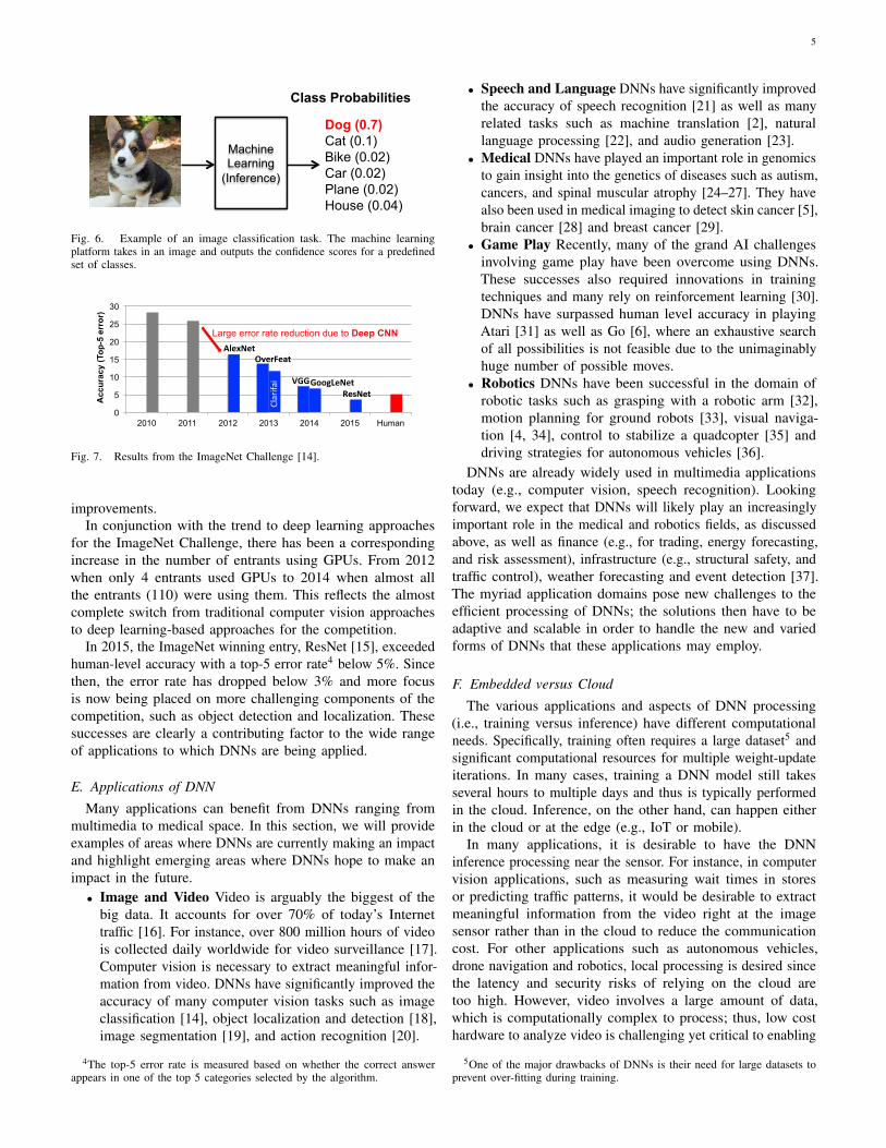
Fig. 6. Example of an image classification task. The machine learningplatform takes in an image and outputs the confidence scores for a predefinedset of classes.

0

5

10

15

20

25

30

2010 2011 2012 2013 2014 2015 Human

Acc

urac

y (T

op-5

err

or)

AlexNetOverFeat

GoogLeNetResNet

Clarifa

i VGG

Large error rate reduction due to Deep CNN

Fig. 7. Results from the ImageNet Challenge [14].

improvements.In conjunction with the trend to deep learning approaches

for the ImageNet Challenge, there has been a correspondingincrease in the number of entrants using GPUs. From 2012when only 4 entrants used GPUs to 2014 when almost allthe entrants (110) were using them. This reflects the almostcomplete switch from traditional computer vision approachesto deep learning-based approaches for the competition.

In 2015, the ImageNet winning entry, ResNet [15], exceededhuman-level accuracy with a top-5 error rate4 below 5%. Sincethen, the error rate has dropped below 3% and more focusis now being placed on more challenging components of thecompetition, such as object detection and localization. Thesesuccesses are clearly a contributing factor to the wide rangeof applications to which DNNs are being applied.

E. Applications of DNN

Many applications can benefit from DNNs ranging frommultimedia to medical space. In this section, we will provideexamples of areas where DNNs are currently making an impactand highlight emerging areas where DNNs hope to make animpact in the future.

• Image and Video Video is arguably the biggest of thebig data. It accounts for over 70% of today’s Internettraffic [16]. For instance, over 800 million hours of videois collected daily worldwide for video surveillance [17].Computer vision is necessary to extract meaningful infor-mation from video. DNNs have significantly improved theaccuracy of many computer vision tasks such as imageclassification [14], object localization and detection [18],image segmentation [19], and action recognition [20].

4The top-5 error rate is measured based on whether the correct answerappears in one of the top 5 categories selected by the algorithm.

• Speech and Language DNNs have significantly improvedthe accuracy of speech recognition [21] as well as manyrelated tasks such as machine translation [2], naturallanguage processing [22], and audio generation [23].

• Medical DNNs have played an important role in genomicsto gain insight into the genetics of diseases such as autism,cancers, and spinal muscular atrophy [24–27]. They havealso been used in medical imaging to detect skin cancer [5],brain cancer [28] and breast cancer [29].

• Game Play Recently, many of the grand AI challengesinvolving game play have been overcome using DNNs.These successes also required innovations in trainingtechniques and many rely on reinforcement learning [30].DNNs have surpassed human level accuracy in playingAtari [31] as well as Go [6], where an exhaustive searchof all possibilities is not feasible due to the unimaginablyhuge number of possible moves.

• Robotics DNNs have been successful in the domain ofrobotic tasks such as grasping with a robotic arm [32],motion planning for ground robots [33], visual naviga-tion [4, 34], control to stabilize a quadcopter [35] anddriving strategies for autonomous vehicles [36].

DNNs are already widely used in multimedia applicationstoday (e.g., computer vision, speech recognition). Lookingforward, we expect that DNNs will likely play an increasinglyimportant role in the medical and robotics fields, as discussedabove, as well as finance (e.g., for trading, energy forecasting,and risk assessment), infrastructure (e.g., structural safety, andtraffic control), weather forecasting and event detection [37].The myriad application domains pose new challenges to theefficient processing of DNNs; the solutions then have to beadaptive and scalable in order to handle the new and variedforms of DNNs that these applications may employ.

F. Embedded versus Cloud

The various applications and aspects of DNN processing(i.e., training versus inference) have different computationalneeds. Specifically, training often requires a large dataset5 andsignificant computational resources for multiple weight-updateiterations. In many cases, training a DNN model still takesseveral hours to multiple days and thus is typically performedin the cloud. Inference, on the other hand, can happen eitherin the cloud or at the edge (e.g., IoT or mobile).

In many applications, it is desirable to have the DNNinference processing near the sensor. For instance, in computervision applications, such as measuring wait times in storesor predicting traffic patterns, it would be desirable to extractmeaningful information from the video right at the imagesensor rather than in the cloud to reduce the communicationcost. For other applications such as autonomous vehicles,drone navigation and robotics, local processing is desired sincethe latency and security risks of relying on the cloud aretoo high. However, video involves a large amount of data,which is computationally complex to process; thus, low costhardware to analyze video is challenging yet critical to enabling

5One of the major drawbacks of DNNs is their need for large datasets toprevent over-fitting during training.

6

Feed Forward Recurrent

(a) Feedforward versus feedback (re-current) networks

Fully-Connected Sparsely-Connected

(b) Fully connected versus sparse

Fig. 8. Different types of neural networks (Figure adopted from [7]).

these applications. Speech recognition enables us to seamlesslyinteract with electronic devices, such as smartphones. Whilecurrently most of the processing for applications such as AppleSiri and Amazon Alexa voice services is in the cloud, it isstill desirable to perform the recognition on the device itself toreduce latency and dependency on connectivity, and to improveprivacy and security.

Many of the embedded platforms that perform DNN infer-ence have stringent energy consumption, compute and memorycost limitations; efficient processing of DNNs have thus becomeof prime importance under these constraints. Therefore, in thisarticle, we will focus on the compute requirements for inferencerather than training.

III. OVERVIEW OF DNNS

DNNs come in a wide variety of shapes and sizes dependingon the application. The popular shapes and sizes are alsoevolving rapidly to improve accuracy and efficiency. In allcases, the input to a DNN is a set of values representing theinformation to be analyzed by the network. For instance, thesevalues can be pixels of an image, sampled amplitudes of anaudio wave or the numerical representation of the state of somesystem or game.

The networks that process the input come in two majorforms: feed forward and recurrent as shown in Fig. 8(a). Infeed-forward networks all of the computation is performed as asequence of operations on the outputs of a previous layer. Thefinal set of operations generates the output of the network, forexample a probability that an image contains a particular object,the probability that an audio sequence contains a particularword, a bounding box in an image around an object or theproposed action that should be taken. In such DNNs, thenetwork has no memory and the output for an input is alwaysthe same irrespective of the sequence of inputs previously givento the network.

In contrast, recurrent neural networks (RNNs), of whichLong Short-Term Memory networks (LSTMs) [38] are apopular variant, have internal memory to allow long-termdependencies to affect the output. In these networks, someintermediate operations generate values that are stored internallyin the network and used as inputs to other operations inconjunction with the processing of a later input. In this article,we will focus on feed-forward networks since (1) the majorcomputation in RNNs is still the weighted sum, which iscovered by the feed-forward networks, and (2) to-date little

attention has been given to hardware acceleration specificallyfor RNNs.

DNNs can be composed solely of fully-connected (FC)layers (also referred to as multi-layer perceptrons, or MLP)as shown in the leftmost layer of Fig. 8(b). In a FC layer,all output activations are composed of a weighted sum ofall input activations (i.e., all outputs are connected to allinputs). This requires a significant amount of storage andcomputation. Thankfully, in many applications, we can removesome connections between the activations by setting the weightsto zero without affecting accuracy. This results in a sparsely-connected layer. A sparsely connected layer is illustrated inthe rightmost layer of Fig. 8(b).

We can also make the computation more efficient by limitingthe number of weights that contribute to an output. This sort ofstructured sparsity can arise if each output is only a functionof a fixed-size window of inputs. Even further efficiency canbe gained if the same set of weights are used in the calculationof every output. This repeated use of the same weight values iscalled weight sharing and can significantly reduce the storagerequirements for weights.

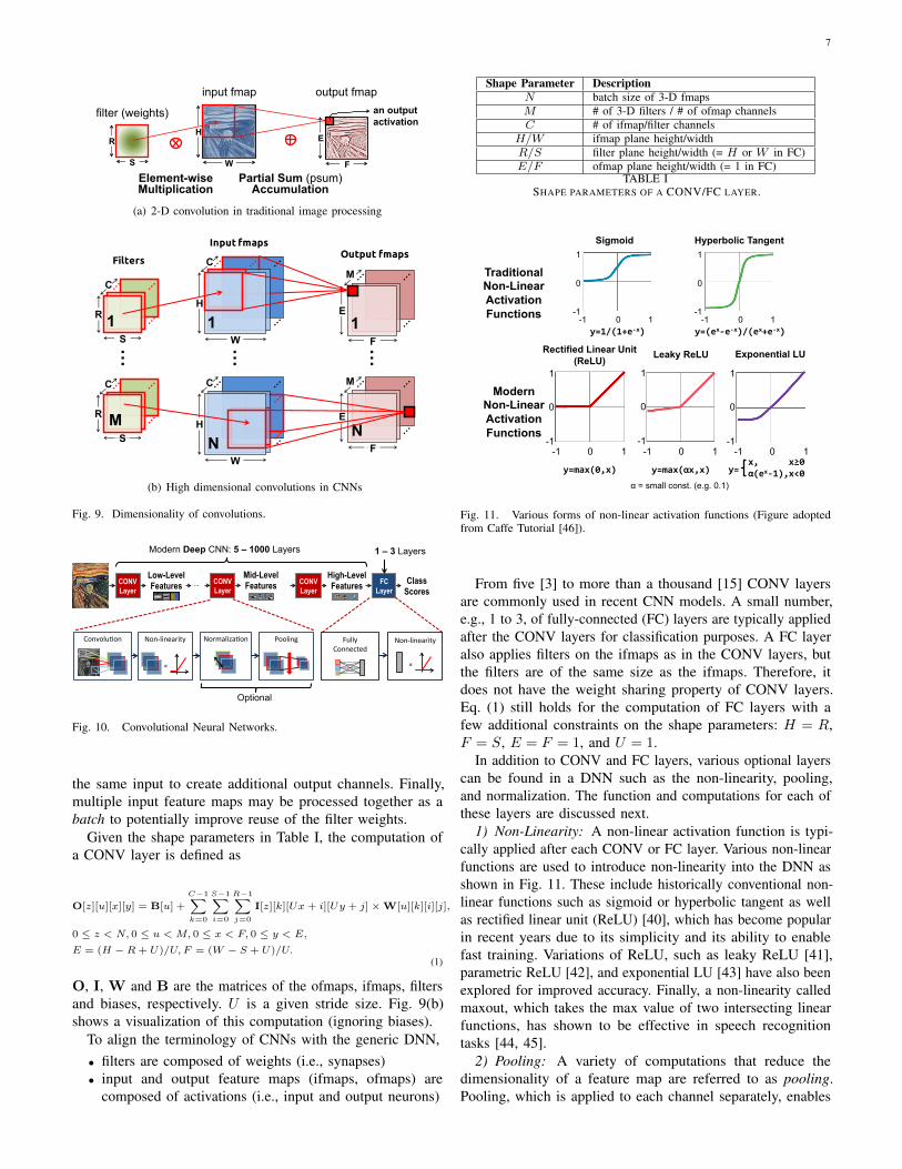
An extremely popular windowed and weight-shared DNNlayer arises by structuring the computation as a convolution,as shown in Fig. 9(a), where the weighted sum for each outputactivation is computed using only a small neighborhood of inputactivations (i.e., all weights beyond beyond the neighborhoodare set to zero), and where the same set of weights are shared forevery output (i.e., the filter is space invariant). Such convolution-based layers are referred to as convolutional (CONV) layers. 6

A. Convolutional Neural Networks (CNNs)

A common form of DNNs is Convolutional Neural Nets(CNNs), which are composed of multiple CONV layers asshown in Fig. 10. In such networks, each layer generates asuccessively higher-level abstraction of the input data, calleda feature map (fmap), which preserves essential yet uniqueinformation. Modern CNNs are able to achieve superior per-formance by employing a very deep hierarchy of layers. CNNare widely used in a variety of applications including imageunderstanding [3], speech recognition [39], game play [6],robotics [32], etc. This paper will focus on its use in imageprocessing, specifically for the task of image classification [3].

Each of the CONV layers in CNN is primarily composed ofhigh-dimensional convolutions as shown in Fig. 9(b). In thiscomputation, the input activations of a layer are structured asa set of 2-D input feature maps (ifmaps), each of which iscalled a channel. Each channel is convolved with a distinct2-D filter from the stack of filters, one for each channel; thisstack of 2-D filters is often referred to as a single 3-D filter.The results of the convolution at each point are summed acrossall the channels. In addition, a 1-D bias can be added to thefiltering results, but some recent networks [15] remove itsusage from parts of the layers. The result of this computationis the output activations that comprise one channel of outputfeature map (ofmap). Additional 3-D filters can be used on

6Note: the structured sparsity in CONV layers is orthogonal to the sparsitythat occurs from network pruning as described in Section VII-B2.

7

R

filter (weights)

S

E

F Partial Sum (psum)

Accumulation

input fmap output fmap

Element-wise Multiplication

H

W

an output activation

(a) 2-D convolution in traditional image processing

Input fmaps

FiltersOutput fmaps

R

S

C

…

H

W

C

…

E

F

M

E

F

M…

R

S

C

H

W

C

1

N

1

M

1

N

(b) High dimensional convolutions in CNNs

Fig. 9. Dimensionality of convolutions.

Modern Deep CNN: 5 – 1000 Layers

Class Scores

FC Layer

CONV Layer

Low-Level Features CONV

Layer

High-Level Features …

1 – 3 Layers

Convolu'on Non-linearity

×

Normaliza'on Pooling

Optional

FullyConnected

×

Non-linearity

CONV Layer

Mid-Level Features

Fig. 10. Convolutional Neural Networks.

the same input to create additional output channels. Finally,multiple input feature maps may be processed together as abatch to potentially improve reuse of the filter weights.

Given the shape parameters in Table I, the computation ofa CONV layer is defined as

O[z][u][x][y] = B[u] +

C−1∑k=0

S−1∑i=0

R−1∑j=0

I[z][k][Ux + i][Uy + j] × W[u][k][i][j],

0 ≤ z < N, 0 ≤ u < M, 0 ≤ x < F, 0 ≤ y < E,

E = (H − R + U)/U, F = (W − S + U)/U.(1)

O, I, W and B are the matrices of the ofmaps, ifmaps, filtersand biases, respectively. U is a given stride size. Fig. 9(b)shows a visualization of this computation (ignoring biases).

To align the terminology of CNNs with the generic DNN,• filters are composed of weights (i.e., synapses)• input and output feature maps (ifmaps, ofmaps) are

composed of activations (i.e., input and output neurons)

Shape Parameter DescriptionN batch size of 3-D fmapsM # of 3-D filters / # of ofmap channelsC # of ifmap/filter channels

H/W ifmap plane height/widthR/S filter plane height/width (= H or W in FC)E/F ofmap plane height/width (= 1 in FC)

TABLE ISHAPE PARAMETERS OF A CONV/FC LAYER.

Sigmoid 1

-1

0

0 1 -1 y=1/(1+e-x)

Hyperbolic Tangent 1

-1

0

0 1 -1 y=(ex-e-x)/(ex+e-x)

Rectified Linear Unit (ReLU)

1

-1

0

0 1 -1

y=max(0,x)

Leaky ReLU

1

-1

0

0 1 -1

y=max(αx,x)

Exponential LU

1

-1

0

0 1 -1 x,α(ex-1),

x≥0x<0y=

α = small const. (e.g. 0.1)

Traditional Non-Linear Activation Functions

Modern Non-Linear Activation Functions

Fig. 11. Various forms of non-linear activation functions (Figure adoptedfrom Caffe Tutorial [46]).

From five [3] to more than a thousand [15] CONV layersare commonly used in recent CNN models. A small number,e.g., 1 to 3, of fully-connected (FC) layers are typically appliedafter the CONV layers for classification purposes. A FC layeralso applies filters on the ifmaps as in the CONV layers, butthe filters are of the same size as the ifmaps. Therefore, itdoes not have the weight sharing property of CONV layers.Eq. (1) still holds for the computation of FC layers with afew additional constraints on the shape parameters: H = R,F = S, E = F = 1, and U = 1.

In addition to CONV and FC layers, various optional layerscan be found in a DNN such as the non-linearity, pooling,and normalization. The function and computations for each ofthese layers are discussed next.

1) Non-Linearity: A non-linear activation function is typi-cally applied after each CONV or FC layer. Various non-linearfunctions are used to introduce non-linearity into the DNN asshown in Fig. 11. These include historically conventional non-linear functions such as sigmoid or hyperbolic tangent as wellas rectified linear unit (ReLU) [40], which has become popularin recent years due to its simplicity and its ability to enablefast training. Variations of ReLU, such as leaky ReLU [41],parametric ReLU [42], and exponential LU [43] have also beenexplored for improved accuracy. Finally, a non-linearity calledmaxout, which takes the max value of two intersecting linearfunctions, has shown to be effective in speech recognitiontasks [44, 45].

2) Pooling: A variety of computations that reduce thedimensionality of a feature map are referred to as pooling.Pooling, which is applied to each channel separately, enables

8

9 3 5 3

10 32 2 2

1 3 21 9

2 6 11 7

2x2 pooling, stride 2

32 5

6 21

Max pooling Average pooling

18 3

3 12

Fig. 12. Various forms of pooling (Figure adopted from Caffe Tutorial [46]).

the network to be robust and invariant to small shifts anddistortions. Pooling combines, or pools, a set of values inits receptive field into a smaller number of values. It can beconfigured based on the size of its receptive field (e.g., 2×2)and pooling operation (e.g., max or average), as shown inFig. 12. Typically pooling occurs on non-overlapping blocks(i.e., the stride is equal to the size of the pooling). Usually astride of greater than one is used such that there is a reductionin the dimension of the representation (i.e., feature map).

3) Normalization: Controlling the input distribution acrosslayers can help to significantly speed up training and improveaccuracy. Accordingly, the distribution of the layer inputactivations (σ, µ) are normalized such that it has a zero meanand a unit standard deviation. In batch normalization (BN),the normalized value is further scaled and shifted, as shownin Eq. (2), where the parameters (γ, β) are learned fromtraining [47]. ε is a small constant to avoid numerical problems.Prior to this, local response normalization (LRN) [3] wasused, which was inspired by lateral inhibition in neurobiologywhere excited neurons (i.e., high value activations) shouldsubdue its neighbors (i.e., cause low value activations); however,BN is now considered standard practice in the design ofCNNs while LRN is mostly deprecated. Note that while LRNusually is performed after the non-linear function, BN is mostlyperformed between the CONV or FC layer and the non-linearfunction.

y =x− µ√σ2 + ε

γ + β (2)

B. Popular DNN Models

Many DNN models have been developed over the pasttwo decades. Each of these models has a different ‘networkarchitecture’ in terms of number of layers, layer types, layershapes (i.e., filter size, number of channels and filters), andconnections between layers. Understanding these variationsand trends is important for incorporating the right flexibilityin any efficient DNN engine.

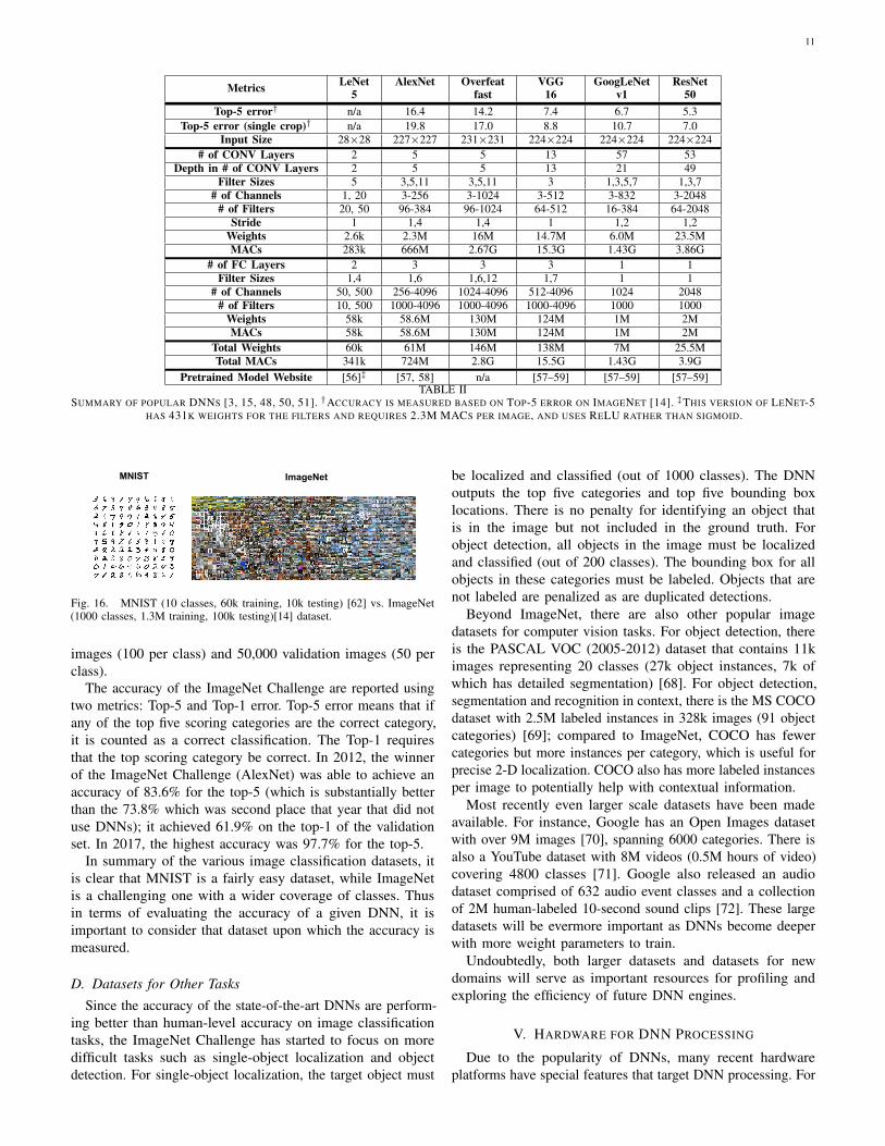
In this section, we will give an overview of various popularDNNs such as LeNet [48] as well as those that competed inand/or won the ImageNet Challenge [14] as shown in Fig. 7,most of whose models with pre-trained weights are publiclyavailable for download; the DNN models are summarized inTable II. Two results for top-5 error results are reported. In thefirst row, the accuracy is boosted by using multiple crops fromthe image and an ensemble of multiple trained models (i.e.,the DNN needs to be run several times); these results wereused to compete in the ImageNet Challenge. The second rowreports the accuracy if only a single crop was used (i.e., the

DNN is run only once), which is more consistent with whatwould likely be deployed in real-time and/or energy-constrainedapplications.

LeNet [11] was one of the first CNN approaches introducedin 1989. It was designed for the task of digit classification ingrayscale images of size 28×28. The most well known version,LeNet-5, contains two CONV layers and two FC layers [48].Each CONV layer uses filters of size 5×5 (1 channel per filter)with 6 filters in the first layer and 16 filters in the second layer.Average pooling of 2×2 is used after each convolution and asigmoid is used for the non-linearity. In total, LeNet requires60k weights and 341k multiply-and-accumulates (MACs) perimage. LeNet led to CNNs’ first commercial success, as it wasdeployed in ATMs to recognize digits for check deposits.

AlexNet [3] was the first CNN to win the ImageNet Challengein 2012. It consists of five CONV layers and three FC layers.Within each CONV layer, there are 96 to 384 filters and thefilter size ranges from 3×3 to 11×11, with 3 to 256 channelseach. In the first layer, the 3 channels of the filter correspondto the red, green and blue components of the input image.A ReLU non-linearity is used in each layer. Max pooling of3×3 is applied to the outputs of layers 1, 2 and 5. To reducecomputation, a stride of 4 is used at the first layer of thenetwork. AlexNet introduced the use of LRN in layers 1 and2 before the max pooling, though LRN is no longer popularin later CNN models. One important factor that differentiatesAlexNet from LeNet is that the number of weights is muchlarger and the shapes vary from layer to layer. To reduce theamount of weights and computation in the second CONV layer,the 96 output channels of the first layer are split into two groupsof 48 input channels for the second layer, such that the filters inthe second layer only have 48 channels. Similarly, the weightsin fourth and fifth layer are also split into two groups. In total,AlexNet requires 61M weights and 724M MACs to processone 227×227 input image.

Overfeat [49] has a very similar architecture to AlexNet withfive CONV layers and three FC layers. The main differencesare that the number of filters is increased for layers 3 (384to 512), 4 (384 to 1024), and 5 (256 to 1024), layer 2 is notsplit into two groups, the first fully connected layer only has3072 channels rather than 4096, and the input size is 231×231rather than 227×227. As a result, the number of weights growsto 146M and the number of MACs grows to 2.8G per image.Overfeat has two different models: fast (described here) andaccurate. The accurate model used in the ImageNet Challengegives a 0.65% lower top-5 error rate than the fast model at thecost of 1.9× more MACs

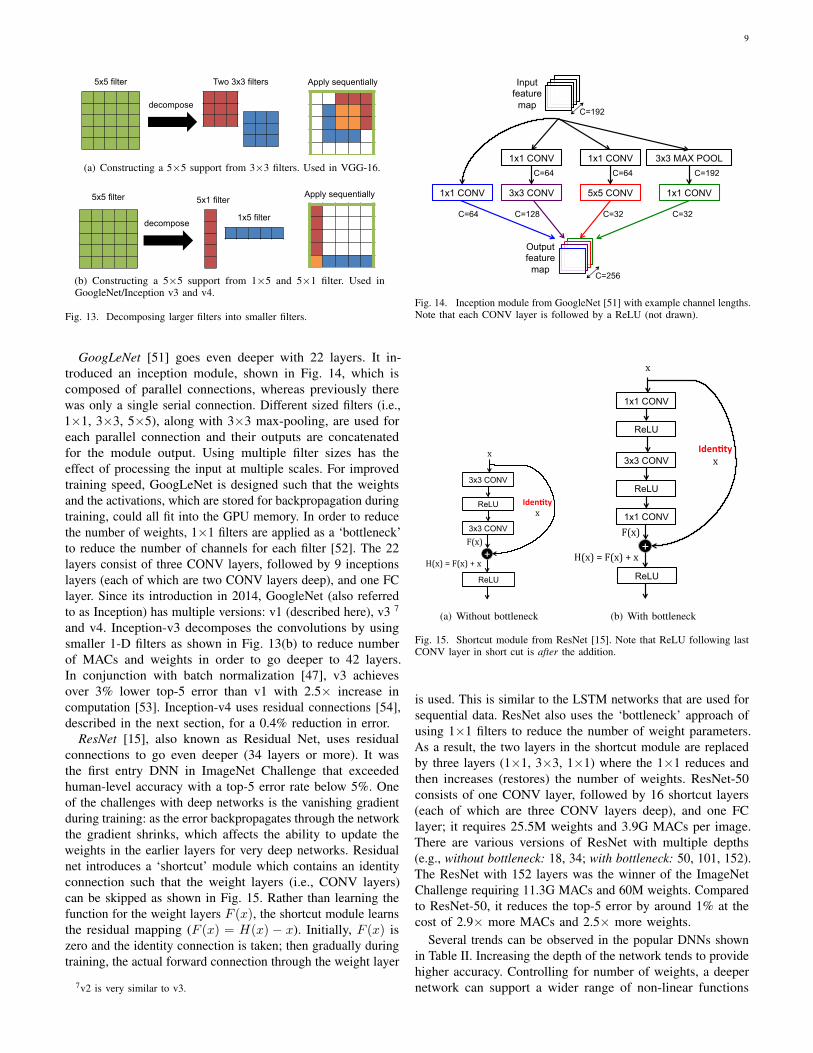
VGG-16 [50] goes deeper to 16 layers consisting of 13CONV layers and 3 FC layers. In order to balance out thecost of going deeper, larger filters (e.g., 5×5) are built frommultiple smaller filters (e.g., 3×3), which have fewer weights,to achieve the same receptive fields as shown in Fig. 13(a).As a result, all CONV layers have the same filter size of 3×3.In total, VGG-16 requires 138M weights and 15.5G MACsto process one 224×224 input image. VGG has two differentmodels: VGG-16 (described here) and VGG-19. VGG-19 givesa 0.1% lower top-5 error rate than VGG-16 at the cost of1.27× more MACs.

9

5x5 filter Two 3x3 filters

decompose

Apply sequentially

(a) Constructing a 5×5 support from 3×3 filters. Used in VGG-16.

decompose

5x5 filter 5x1 filter

1x5 filter

Apply sequentially

(b) Constructing a 5×5 support from 1×5 and 5×1 filter. Used inGoogleNet/Inception v3 and v4.

Fig. 13. Decomposing larger filters into smaller filters.

GoogLeNet [51] goes even deeper with 22 layers. It in-troduced an inception module, shown in Fig. 14, which iscomposed of parallel connections, whereas previously therewas only a single serial connection. Different sized filters (i.e.,1×1, 3×3, 5×5), along with 3×3 max-pooling, are used foreach parallel connection and their outputs are concatenatedfor the module output. Using multiple filter sizes has theeffect of processing the input at multiple scales. For improvedtraining speed, GoogLeNet is designed such that the weightsand the activations, which are stored for backpropagation duringtraining, could all fit into the GPU memory. In order to reducethe number of weights, 1×1 filters are applied as a ‘bottleneck’to reduce the number of channels for each filter [52]. The 22layers consist of three CONV layers, followed by 9 inceptionslayers (each of which are two CONV layers deep), and one FClayer. Since its introduction in 2014, GoogleNet (also referredto as Inception) has multiple versions: v1 (described here), v3 7

and v4. Inception-v3 decomposes the convolutions by usingsmaller 1-D filters as shown in Fig. 13(b) to reduce numberof MACs and weights in order to go deeper to 42 layers.In conjunction with batch normalization [47], v3 achievesover 3% lower top-5 error than v1 with 2.5× increase incomputation [53]. Inception-v4 uses residual connections [54],described in the next section, for a 0.4% reduction in error.

ResNet [15], also known as Residual Net, uses residualconnections to go even deeper (34 layers or more). It wasthe first entry DNN in ImageNet Challenge that exceededhuman-level accuracy with a top-5 error rate below 5%. Oneof the challenges with deep networks is the vanishing gradientduring training: as the error backpropagates through the networkthe gradient shrinks, which affects the ability to update theweights in the earlier layers for very deep networks. Residualnet introduces a ‘shortcut’ module which contains an identityconnection such that the weight layers (i.e., CONV layers)can be skipped as shown in Fig. 15. Rather than learning thefunction for the weight layers F (x), the shortcut module learnsthe residual mapping (F (x) = H(x) − x). Initially, F (x) iszero and the identity connection is taken; then gradually duringtraining, the actual forward connection through the weight layer

7v2 is very similar to v3.

1x1 CONV 3x3 CONV 5x5 CONV 1x1 CONV

1x1 CONV 1x1 CONV 3x3 MAX POOL

Input feature

map

Output feature

map

C=64 C=192

C=32 C=32 C=128 C=64

C=192

C=64

C=256

Fig. 14. Inception module from GoogleNet [51] with example channel lengths.Note that each CONV layer is followed by a ReLU (not drawn).

3x3 CONV

ReLU

ReLU

3x3 CONV

+

x

F(x)

H(x)=F(x)+x

Iden%tyx

(a) Without bottleneck

3x3 CONV

ReLU

ReLU

1x1 CONV

+

x

F(x)

H(x)=F(x)+x

1x1 CONV

ReLU

Iden%tyx

(b) With bottleneck

Fig. 15. Shortcut module from ResNet [15]. Note that ReLU following lastCONV layer in short cut is after the addition.

is used. This is similar to the LSTM networks that are used forsequential data. ResNet also uses the ‘bottleneck’ approach ofusing 1×1 filters to reduce the number of weight parameters.As a result, the two layers in the shortcut module are replacedby three layers (1×1, 3×3, 1×1) where the 1×1 reduces andthen increases (restores) the number of weights. ResNet-50consists of one CONV layer, followed by 16 shortcut layers(each of which are three CONV layers deep), and one FClayer; it requires 25.5M weights and 3.9G MACs per image.There are various versions of ResNet with multiple depths(e.g., without bottleneck: 18, 34; with bottleneck: 50, 101, 152).The ResNet with 152 layers was the winner of the ImageNetChallenge requiring 11.3G MACs and 60M weights. Comparedto ResNet-50, it reduces the top-5 error by around 1% at thecost of 2.9× more MACs and 2.5× more weights.

Several trends can be observed in the popular DNNs shownin Table II. Increasing the depth of the network tends to providehigher accuracy. Controlling for number of weights, a deepernetwork can support a wider range of non-linear functions

10

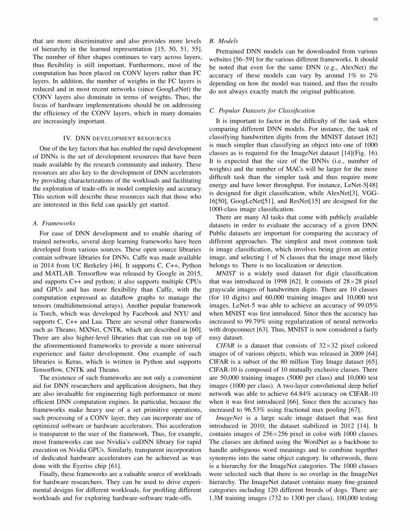
that are more discriminative and also provides more levelsof hierarchy in the learned representation [15, 50, 51, 55].The number of filter shapes continues to vary across layers,thus flexibility is still important. Furthermore, most of thecomputation has been placed on CONV layers rather than FClayers. In addition, the number of weights in the FC layers isreduced and in most recent networks (since GoogLeNet) theCONV layers also dominate in terms of weights. Thus, thefocus of hardware implementations should be on addressingthe efficiency of the CONV layers, which in many domainsare increasingly important.

IV. DNN DEVELOPMENT RESOURCES

One of the key factors that has enabled the rapid developmentof DNNs is the set of development resources that have beenmade available by the research community and industry. Theseresources are also key to the development of DNN acceleratorsby providing characterizations of the workloads and facilitatingthe exploration of trade-offs in model complexity and accuracy.This section will describe these resources such that those whoare interested in this field can quickly get started.

A. Frameworks

For ease of DNN development and to enable sharing oftrained networks, several deep learning frameworks have beendeveloped from various sources. These open source librariescontain software libraries for DNNs. Caffe was made availablein 2014 from UC Berkeley [46]. It supports C, C++, Pythonand MATLAB. Tensorflow was released by Google in 2015,and supports C++ and python; it also supports multiple CPUsand GPUs and has more flexibility than Caffe, with thecomputation expressed as dataflow graphs to manage thetensors (multidimensional arrays). Another popular frameworkis Torch, which was developed by Facebook and NYU andsupports C, C++ and Lua. There are several other frameworkssuch as Theano, MXNet, CNTK, which are described in [60].There are also higher-level libraries that can run on top ofthe aforementioned frameworks to provide a more universalexperience and faster development. One example of suchlibraries is Keras, which is written in Python and supportsTensorflow, CNTK and Theano.

The existence of such frameworks are not only a convenientaid for DNN researchers and application designers, but theyare also invaluable for engineering high performance or moreefficient DNN computation engines. In particular, because theframeworks make heavy use of a set primitive operations,such processing of a CONV layer, they can incorporate use ofoptimized software or hardware accelerators. This accelerationis transparent to the user of the framework. Thus, for example,most frameworks can use Nvidia’s cuDNN library for rapidexecution on Nvidia GPUs. Similarly, transparent incorporationof dedicated hardware accelerators can be achieved as wasdone with the Eyeriss chip [61].

Finally, these frameworks are a valuable source of workloadsfor hardware researchers. They can be used to drive experi-mental designs for different workloads, for profiling differentworkloads and for exploring hardware-software trade-offs.

B. Models

Pretrained DNN models can be downloaded from variouswebsites [56–59] for the various different frameworks. It shouldbe noted that even for the same DNN (e.g., AlexNet) theaccuracy of these models can vary by around 1% to 2%depending on how the model was trained, and thus the resultsdo not always exactly match the original publication.

C. Popular Datasets for Classification

It is important to factor in the difficulty of the task whencomparing different DNN models. For instance, the task ofclassifying handwritten digits from the MNIST dataset [62]is much simpler than classifying an object into one of 1000classes as is required for the ImageNet dataset [14](Fig. 16).It is expected that the size of the DNNs (i.e., number ofweights) and the number of MACs will be larger for the moredifficult task than the simpler task and thus require moreenergy and have lower throughput. For instance, LeNet-5[48]is designed for digit classification, while AlexNet[3], VGG-16[50], GoogLeNet[51], and ResNet[15] are designed for the1000-class image classification.

There are many AI tasks that come with publicly availabledatasets in order to evaluate the accuracy of a given DNN.Public datasets are important for comparing the accuracy ofdifferent approaches. The simplest and most common taskis image classification, which involves being given an entireimage, and selecting 1 of N classes that the image most likelybelongs to. There is no localization or detection.

MNIST is a widely used dataset for digit classificationthat was introduced in 1998 [62]. It consists of 28×28 pixelgrayscale images of handwritten digits. There are 10 classes(for 10 digits) and 60,000 training images and 10,000 testimages. LeNet-5 was able to achieve an accuracy of 99.05%when MNIST was first introduced. Since then the accuracy hasincreased to 99.79% using regularization of neural networkswith dropconnect [63]. Thus, MNIST is now considered a fairlyeasy dataset.

CIFAR is a dataset that consists of 32×32 pixel coloredimages of of various objects, which was released in 2009 [64].CIFAR is a subset of the 80 million Tiny Image dataset [65].CIFAR-10 is composed of 10 mutually exclusive classes. Thereare 50,000 training images (5000 per class) and 10,000 testimages (1000 per class). A two-layer convolutional deep beliefnetwork was able to achieve 64.84% accuracy on CIFAR-10when it was first introduced [66]. Since then the accuracy hasincreased to 96.53% using fractional max pooling [67].

ImageNet is a large scale image dataset that was firstintroduced in 2010; the dataset stabilized in 2012 [14]. Itcontains images of 256×256 pixel in color with 1000 classes.The classes are defined using the WordNet as a backbone tohandle ambiguous word meanings and to combine togethersynonyms into the same object category. In otherwords, thereis a hierarchy for the ImageNet categories. The 1000 classeswere selected such that there is no overlap in the ImageNethierarchy. The ImageNet dataset contains many fine-grainedcategories including 120 different breeds of dogs. There are1.3M training images (732 to 1300 per class), 100,000 testing

11

Metrics LeNet AlexNet Overfeat VGG GoogLeNet ResNet5 fast 16 v1 50

Top-5 error† n/a 16.4 14.2 7.4 6.7 5.3Top-5 error (single crop)† n/a 19.8 17.0 8.8 10.7 7.0

Input Size 28×28 227×227 231×231 224×224 224×224 224×224# of CONV Layers 2 5 5 13 57 53

Depth in # of CONV Layers 2 5 5 13 21 49Filter Sizes 5 3,5,11 3,5,11 3 1,3,5,7 1,3,7

# of Channels 1, 20 3-256 3-1024 3-512 3-832 3-2048# of Filters 20, 50 96-384 96-1024 64-512 16-384 64-2048

Stride 1 1,4 1,4 1 1,2 1,2Weights 2.6k 2.3M 16M 14.7M 6.0M 23.5MMACs 283k 666M 2.67G 15.3G 1.43G 3.86G

# of FC Layers 2 3 3 3 1 1Filter Sizes 1,4 1,6 1,6,12 1,7 1 1

# of Channels 50, 500 256-4096 1024-4096 512-4096 1024 2048# of Filters 10, 500 1000-4096 1000-4096 1000-4096 1000 1000

Weights 58k 58.6M 130M 124M 1M 2MMACs 58k 58.6M 130M 124M 1M 2M

Total Weights 60k 61M 146M 138M 7M 25.5MTotal MACs 341k 724M 2.8G 15.5G 1.43G 3.9G

Pretrained Model Website [56]‡ [57, 58] n/a [57–59] [57–59] [57–59]TABLE II

SUMMARY OF POPULAR DNNS [3, 15, 48, 50, 51]. †ACCURACY IS MEASURED BASED ON TOP-5 ERROR ON IMAGENET [14]. ‡THIS VERSION OF LENET-5HAS 431K WEIGHTS FOR THE FILTERS AND REQUIRES 2.3M MACS PER IMAGE, AND USES RELU RATHER THAN SIGMOID.

MNIST ImageNet

Fig. 16. MNIST (10 classes, 60k training, 10k testing) [62] vs. ImageNet(1000 classes, 1.3M training, 100k testing)[14] dataset.

images (100 per class) and 50,000 validation images (50 perclass).

The accuracy of the ImageNet Challenge are reported usingtwo metrics: Top-5 and Top-1 error. Top-5 error means that ifany of the top five scoring categories are the correct category,it is counted as a correct classification. The Top-1 requiresthat the top scoring category be correct. In 2012, the winnerof the ImageNet Challenge (AlexNet) was able to achieve anaccuracy of 83.6% for the top-5 (which is substantially betterthan the 73.8% which was second place that year that did notuse DNNs); it achieved 61.9% on the top-1 of the validationset. In 2017, the highest accuracy was 97.7% for the top-5.

In summary of the various image classification datasets, itis clear that MNIST is a fairly easy dataset, while ImageNetis a challenging one with a wider coverage of classes. Thusin terms of evaluating the accuracy of a given DNN, it isimportant to consider that dataset upon which the accuracy ismeasured.

D. Datasets for Other Tasks

Since the accuracy of the state-of-the-art DNNs are perform-ing better than human-level accuracy on image classificationtasks, the ImageNet Challenge has started to focus on moredifficult tasks such as single-object localization and objectdetection. For single-object localization, the target object must

be localized and classified (out of 1000 classes). The DNNoutputs the top five categories and top five bounding boxlocations. There is no penalty for identifying an object thatis in the image but not included in the ground truth. Forobject detection, all objects in the image must be localizedand classified (out of 200 classes). The bounding box for allobjects in these categories must be labeled. Objects that arenot labeled are penalized as are duplicated detections.

Beyond ImageNet, there are also other popular imagedatasets for computer vision tasks. For object detection, thereis the PASCAL VOC (2005-2012) dataset that contains 11kimages representing 20 classes (27k object instances, 7k ofwhich has detailed segmentation) [68]. For object detection,segmentation and recognition in context, there is the MS COCOdataset with 2.5M labeled instances in 328k images (91 objectcategories) [69]; compared to ImageNet, COCO has fewercategories but more instances per category, which is useful forprecise 2-D localization. COCO also has more labeled instancesper image to potentially help with contextual information.

Most recently even larger scale datasets have been madeavailable. For instance, Google has an Open Images datasetwith over 9M images [70], spanning 6000 categories. There isalso a YouTube dataset with 8M videos (0.5M hours of video)covering 4800 classes [71]. Google also released an audiodataset comprised of 632 audio event classes and a collectionof 2M human-labeled 10-second sound clips [72]. These largedatasets will be evermore important as DNNs become deeperwith more weight parameters to train.

Undoubtedly, both larger datasets and datasets for newdomains will serve as important resources for profiling andexploring the efficiency of future DNN engines.

V. HARDWARE FOR DNN PROCESSING

Due to the popularity of DNNs, many recent hardwareplatforms have special features that target DNN processing. For

12

instance, the Intel Knights Landing CPU features special vectorinstructions for deep learning; the Nvidia PASCAL GP100GPU features 16-bit floating point (FP16) arithmetic supportto perform two FP16 operations on a single precision core forfaster deep learning computation. Systems have also been builtspecifically for DNN processing such as Nvidia DGX-1 andFacebook’s Big Basin custom DNN server [73]. DNN inferencehas also been demonstrated on various embedded System-on-Chips (SoC) such as Nvidia Tegra and Samsung Exynos aswell as FPGAs. Accordingly, it’s important to have a goodunderstanding of how the processing is being performed onthese platforms, and how application-specific accelerators canbe designed for DNNs for further improvement in throughputand energy efficiency.

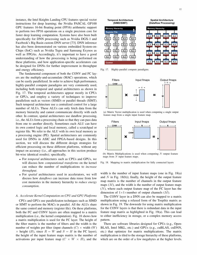
The fundamental component of both the CONV and FC lay-ers are the multiply-and-accumulate (MAC) operations, whichcan be easily parallelized. In order to achieve high performance,highly-parallel compute paradigms are very commonly used,including both temporal and spatial architectures as shown inFig. 17. The temporal architectures appear mostly in CPUsor GPUs, and employ a variety of techniques to improveparallelism such as vectors (SIMD) or parallel threads (SIMT).Such temporal architecture use a centralized control for a largenumber of ALUs. These ALUs can only fetch data from thememory hierarchy and cannot communicate directly with eachother. In contrast, spatial architectures use dataflow processing,i.e., the ALUs form a processing chain so that they can pass datafrom one to another directly. Sometimes each ALU can haveits own control logic and local memory, called a scratchpad orregister file. We refer to the ALU with its own local memory asa processing engine (PE). Spatial architectures are commonlyused for DNNs in ASIC and FPGA-based designs. In thissection, we will discuss the different design strategies forefficient processing on these different platforms, without anyimpact on accuracy (i.e., all approaches in this section producebit-wise identical results); specifically,

• For temporal architectures such as CPUs and GPUs, wewill discuss how computational transforms on the kernelcan reduce the number of multiplications to increasethroughput.

• For spatial architectures used in accelerators, we willdiscuss how dataflows can increase data reuse from lowcost memories in the memory hierarchy to reduce energyconsumption.

A. Accelerate Kernel Computation on CPU and GPU Platforms

CPUs and GPUs use parallelizaton techniques such as SIMDor SIMT to perform the MACs in parallel. All the ALUs sharethe same control and memory (register file). On these platforms,both the FC and CONV layers are often mapped to a matrixmultiplication (i.e., the kernel computation). Fig. 18 shows howa matrix multiplication is used for the FC layer. The height ofthe filter matrix is the number of filters and the width is thenumber of weights per filter (input channels (C) × width (W )× height (H), since R = W and S = H in the FC layer);the height of the input feature maps matrix is the number ofactivations per input feature map (C × W × H), and the

Temporal Architecture (SIMD/SIMT)

Spatial Architecture (Dataflow Processing)

Register File

Memory Hierarchy

ALU

ALU

ALU

ALU

ALU

ALU

ALU

ALU

ALU

ALU

ALU

ALU

ALU

ALU

ALU

ALU

Control

Memory Hierarchy

ALU ALU ALU ALU

ALU ALU ALU ALU

ALU ALU ALU ALU

ALU ALU ALU ALU

Fig. 17. Highly-parallel compute paradigms.

M

CHW

CHW

1

Filters Input fmaps

×

1 Output fmaps

M =

(a) Matrix Vector multiplication is used when computing a single outputfeature map from a single input feature map.

M

CHW

CHW

N

Filters Input fmaps

×

N

Output fmaps

M =

(b) Matrix Multiplications is used when computing N output featuremaps from N input feature maps.

Fig. 18. Mapping to matrix multiplication for fully connected layers

width is the number of input feature maps (one in Fig. 18(a)and N in Fig. 18(b)); finally, the height of the output featuremap matrix is the number of channels in the output featuremaps (M ), and the width is the number of output feature maps(N ), where each output feature map of the FC layer has thedimension of 1×1×number of output channels (M ).

The CONV layer in a DNN can also be mapped to a matrixmultiplication using a relaxed form of the Toeplitz matrix asshown in Fig. 19. The downside for using matrix multiplicationfor the CONV layers is that there is redundant data in the inputfeature map matrix as highlighted in Fig. 19(a). This can leadto either inefficiency in storage, or a complex memory accesspattern.

There are software libraries designed for CPUs (e.g., Open-BLAS, Intel MKL, etc.) and GPUs (e.g., cuBLAS, cuDNN,etc.) that optimize for matrix multiplications. The matrixmultiplication is tiled to the storage hierarchy of these platforms,which are on the order of a few megabytes at the higher levels.

13

1 2 34 5 67 8 9

1 23 4

Filter Input Fmap Output Fmap

* = 1 23 4

1 2 3 41 2 4 52 3 5 64 5 7 85 6 8 9

1 2 3 4 × =

Toeplitz Matrix (w/ redundant data)

Convolution:

Matrix Mult:

(a) Mapping convolution to Toeplitz matrix

= 1 2 3 41 2 3 4

1 2 3 41 2 3 4

1245

2356

4578

5689

1245

2356

4578

5689

1 21 2 3 4

3 4×

Toeplitz Matrix (w/ redundant data) Chnl 1 Chnl 2

Filter 1 Filter 2

Chnl 1

Chnl 2

Chnl 1 Chnl 2

(b) Extend Toeplitz matrix to multiple channels and filters

Fig. 19. Mapping to matrix multiplication for convolutional layers.

The matrix multiplications on these platforms can be furthersped up by applying computational transforms to the data toreduce the number of multiplications, while still giving thesame bit-wise result. Often this can come at a cost of increasednumber of additions and a more irregular data access pattern.

Fast Fourier Transform (FFT) [10, 74] is a well knownapproach, shown in Fig. 20 that reduces the number ofmultiplications from O(N2

oN2f ) to O(N2

o log2No), where theoutput size is No × No and the filter size is Nf × Nf . Toperform the convolution, we take the FFT of the filter andinput feature map, and then perform the multiplication inthe frequency domain; we then apply an inverse FFT to theresulting product to recover the output feature map in thespatial domain. However, there are several drawbacks to usingFFT: (1) the benefits of FFTs decrease with filter size; (2) thesize of the FFT is dictated by the output feature map size whichis often much larger than the filter; (3) the coefficients in thefrequency domain are complex. As a result, while FFT reducescomputation, it requires larger storage capacity and bandwidth.Finally, a popular approach for reducing complexity is to makethe weights sparse, which will be discussed in Section VII-B2;using FFTs makes it difficult for this sparsity to be exploited.

Several optimizations can be performed on FFT to make itmore effective for DNNs. To reduce the number of operations,the FFT of the filter can be precomputed and stored. In addition,the FFT of the input feature map can be computed once andused to generate multiple channels in the output feature map.Finally, since an image contains only real values, its FourierTransform is symmetric and this can be exploited to reducestorage and computation cost.

Other approaches include Strassen [75] and Winograd [76],which rearrange the computation such that the number ofmultiplications reduce from O(N3) to O(N2.807) and by 2.25×

R

filter (weights)

S

E

F

input fmap output fmap

H

W

an output activation

* =

FFT(W)

FFT

FFT(I) X = FFT(0)

FFT

IFFT

Fig. 20. FFT to accelerate DNN.

ALU filter weight fmap activation

partial sum updated partial sum

Memory Read Memory Write MAC*

* multiply-and-accumulate

Fig. 21. Read and write access per MAC.

for a 3×3 filter, respectively, at the cost of reduced numeri-cal stability, increased storage requirements, and specializedprocessing depending on the size of the filter.

In practice, different algorithms might be used for differentlayer shapes and sizes (e.g., FFT for filters greater than 5×5,and Winograd for filters 3×3 and below). Existing platformlibraries, such as MKL and cuDNN, dynamically chose theappropriate algorithm for a given shape and size [77, 78].

B. Energy-Efficient Dataflow for Accelerators

For DNNs, the bottleneck for processing is in the memoryaccess. Each MAC requires three memory reads (for filterweight, fmap activation, and partial sum) and one memorywrite (for the updated partial sum) as shown in Fig. 21. In theworst case, all of the memory accesses have to go through theoff-chip DRAM, which will severely impact both throughputand energy efficiency. For example, in AlexNet, to support its724M MACs, nearly 3000M DRAM accesses will be required.Furthermore, DRAM accesses require up to several orders ofmagnitude higher energy than computation [79].

Accelerators, such as spatial architectures as shown inFig. 17, provide an opportunity to reduce the energy cost ofdata movement by introducing several levels of local memoryhierarchy with different energy cost as shown in Fig. 22. Thisincludes a large global buffer with a size of several hundredkilobytes that connects to DRAM, an inter-PE network thatcan pass data directly between the ALUs, and a register file(RF) within each processing element (PE) with a size of afew kilobytes or less. The multiple levels of memory hierarchyhelp to improve energy efficiency by providing low-cost dataaccesses. For example, fetching the data from the RF orneighbor PEs is going to cost 1 or 2 orders of magnitudelower energy than from DRAM.

Accelerators can be designed to support specialized process-ing dataflows that leverage this memory hierarchy. The dataflow

14

DRAM Global Buffer PE

PE PE

ALU fetch data to run a MAC here

ALU

Buffer ALU

RF ALU

Normalized Energy Cost

200× 6×

PE ALU 2× 1× 1× (Reference)

DRAM ALU

0.5 – 1.0 kB

100 – 500 kB

NoC: 200 – 1000 PEs

Fig. 22. Memory hierarchy and data movement energy [80].

decides what data gets read into which level of the memoryhierarchy and when are they getting processed. Since there isno randomness in the processing of DNNs, it is possible todesign a fixed dataflow that can adapt to the DNN shapes andsizes and optimize for the best energy efficiency. The optimizeddataflow minimizes access from the more energy consuminglevels of the memory hierarchy. Large memories that can storea significant amount of data consume more energy than smallermemories. For instance, DRAM can store gigabytes of data, butconsumes two orders of magnitude higher energy per accessthan a small on-chip memory of a few kilobytes. Thus, everytime a piece of data is moved from an expensive level to alower cost level in terms of energy, we want to reuse that pieceof data as much as possible to minimize subsequent accessesto the expensive levels. The challenge, however, is that thestorage capacity of these low cost memories are limited. Thuswe need to explore different dataflows that maximize reuseunder these constraints.

For DNNs, we investigate dataflows that exploit three formsof input data reuse (convolutional, feature map and filter) asshown in Fig. 23. For convolutional reuse, the same inputfeature map activations and filter weights are used withina given channel, just in different combinations for differentweighted sums. For feature map reuse, multiple filters areapplied to the same feature map, so the input feature mapactivations are used multiple times across filters. Finally, forfilter reuse, when multiple input feature maps are processed atonce (referred to as a batch), the same filter weights are usedmultiple times across input features maps.

If we can harness the three types of data reuse by storingthe data in the local memory hierarchy and accessing themmultiple times without going back to the DRAM, it can savea significant amount of DRAM accesses. For example, inAlexNet, the number of DRAM reads can be reduced by up to500× in the CONV layers. The local memory can also be usedfor partial sum accumulation, so they do not have to reachDRAM. In the best case, if all data reuse and accumulationcan be achieved by the local memory hierarchy, the 3000MDRAM accesses in AlexNet can be reduced to only 61M.

The operation of DNN accelerators is analogous to that ofgeneral-purpose processors as illustrated in Fig. 24 [81]. Inconventional computer systems, the compiler translates the

Filter Reuse Convolutional Reuse Fmap Reuse CONV layers only (sliding window)

CONV and FC layers CONV and FC layers (batch size > 1)

Filter Input Fmap

Filters

2

1

Input Fmap

Filter

2

1

Input Fmaps

Activations Filter weights

Reuse: Activations Reuse: Filter weights Reuse:

Fig. 23. Data reuse opportunities in DNNs [80].

Compilation ExecutionDNN Shape and Size

(Program)

Mapping InputData

ProcessedData

Mapper(Compiler)

DNN Accelerator(Processor)

Dataflow, …(Architecture)

(Binary)

Implementation Details(µArch)

Fig. 24. An analogy between the operation of DNN accelerators (texts inblack) and that of general-purpose processors (texts in red). Figure adoptedfrom [81].

program into machine-readable binary codes for executiongiven the hardware architecture (e.g., x86 or ARM); in theprocessing of DNNs, the mapper translates the DNN shapeand size into a hardware-compatible computation mappingfor execution given the dataflow. While the compiler usuallyoptimizes for performance, the mapper optimizes for energyefficiency.

The following taxonomy (Fig. 25) can be used to classifythe DNN dataflows in recent works [82–93] based on theirdata handling characteristics [80]:

1) Weight stationary (WS): The weight stationary dataflowis designed to minimize the energy consumption of readingweights by maximizing the accesses of weights from the registerfile (RF) at the PE (Fig. 25(a)). Each weight is read fromDRAM into the RF of each PE and stays stationary for furtheraccesses. The processing runs as many MACs that use thesame weight as possible while the weight is present in the RF;it maximizes convolutional and filter reuse of weights. Theinputs and partial sums must move through the spatial arrayand global buffer. The input fmap activations are broadcast toall PEs and then the partial sums are spatially accumulatedacross the PE array.

One example of previous work that implement weightstationary dataflow is nn-X, or neuFlow [85], which useseight 2-D convolution engines for processing a 10×10 filter.There are total 100 MAC units, i.e. PEs, per engine with eachPE having a weight that stays stationary for processing. The

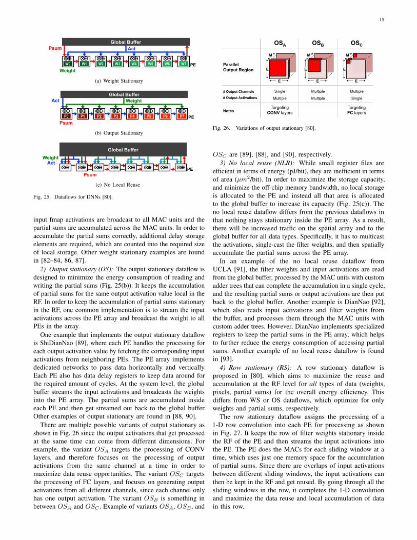
15

Global Buffer

W0 W1 W2 W3 W4 W5 W6 W7

Psum Act

PE Weight

(a) Weight Stationary

Global Buffer

P0 P1 P2 P3 P4 P5 P6 P7

Act Weight

PE Psum

(b) Output Stationary

PE Act

Psum

Global Buffer Weight

(c) No Local Reuse

Fig. 25. Dataflows for DNNs [80].

input fmap activations are broadcast to all MAC units and thepartial sums are accumulated across the MAC units. In order toaccumulate the partial sums correctly, additional delay storageelements are required, which are counted into the required sizeof local storage. Other weight stationary examples are foundin [82–84, 86, 87].

2) Output stationary (OS): The output stationary dataflow isdesigned to minimize the energy consumption of reading andwriting the partial sums (Fig. 25(b)). It keeps the accumulationof partial sums for the same output activation value local in theRF. In order to keep the accumulation of partial sums stationaryin the RF, one common implementation is to stream the inputactivations across the PE array and broadcast the weight to allPEs in the array.

One example that implements the output stationary dataflowis ShiDianNao [89], where each PE handles the processing foreach output activation value by fetching the corresponding inputactivations from neighboring PEs. The PE array implementsdedicated networks to pass data horizontally and vertically.Each PE also has data delay registers to keep data around forthe required amount of cycles. At the system level, the globalbuffer streams the input activations and broadcasts the weightsinto the PE array. The partial sums are accumulated insideeach PE and then get streamed out back to the global buffer.Other examples of output stationary are found in [88, 90].

There are multiple possible variants of output stationary asshown in Fig. 26 since the output activations that get processedat the same time can come from different dimensions. Forexample, the variant OSA targets the processing of CONVlayers, and therefore focuses on the processing of outputactivations from the same channel at a time in order tomaximize data reuse opportunities. The variant OSC targetsthe processing of FC layers, and focuses on generating outputactivations from all different channels, since each channel onlyhas one output activation. The variant OSB is something inbetween OSA and OSC . Example of variants OSA, OSB , and

# Output Channels

# Output Activations

E

E

…

…

… M

OSB

Multiple

Multiple

Notes

E

E

…

…

… M

OSA

Single

Multiple

Targeting CONV layers

E

E

…

…

… M

OSC

Multiple

Single

Targeting FC layers

Parallel Output Region

Fig. 26. Variations of output stationary [80].

OSC are [89], [88], and [90], respectively.3) No local reuse (NLR): While small register files are

efficient in terms of energy (pJ/bit), they are inefficient in termsof area (µm2/bit). In order to maximize the storage capacity,and minimize the off-chip memory bandwidth, no local storageis allocated to the PE and instead all that area is allocatedto the global buffer to increase its capacity (Fig. 25(c)). Theno local reuse dataflow differs from the previous dataflows inthat nothing stays stationary inside the PE array. As a result,there will be increased traffic on the spatial array and to theglobal buffer for all data types. Specifically, it has to multicastthe activations, single-cast the filter weights, and then spatiallyaccumulate the partial sums across the PE array.

In an example of the no local reuse dataflow fromUCLA [91], the filter weights and input activations are readfrom the global buffer, processed by the MAC units with customadder trees that can complete the accumulation in a single cycle,and the resulting partial sums or output activations are then putback to the global buffer. Another example is DianNao [92],which also reads input activations and filter weights fromthe buffer, and processes them through the MAC units withcustom adder trees. However, DianNao implements specializedregisters to keep the partial sums in the PE array, which helpsto further reduce the energy consumption of accessing partialsums. Another example of no local reuse dataflow is foundin [93].

4) Row stationary (RS): A row stationary dataflow isproposed in [80], which aims to maximize the reuse andaccumulation at the RF level for all types of data (weights,pixels, partial sums) for the overall energy efficiency. Thisdiffers from WS or OS dataflows, which optimize for onlyweights and partial sums, respectively.

The row stationary dataflow assigns the processing of a1-D row convolution into each PE for processing as shownin Fig. 27. It keeps the row of filter weights stationary insidethe RF of the PE and then streams the input activations intothe PE. The PE does the MACs for each sliding window at atime, which uses just one memory space for the accumulationof partial sums. Since there are overlaps of input activationsbetween different sliding windows, the input activations canthen be kept in the RF and get reused. By going through all thesliding windows in the row, it completes the 1-D convolutionand maximize the data reuse and local accumulation of datain this row.

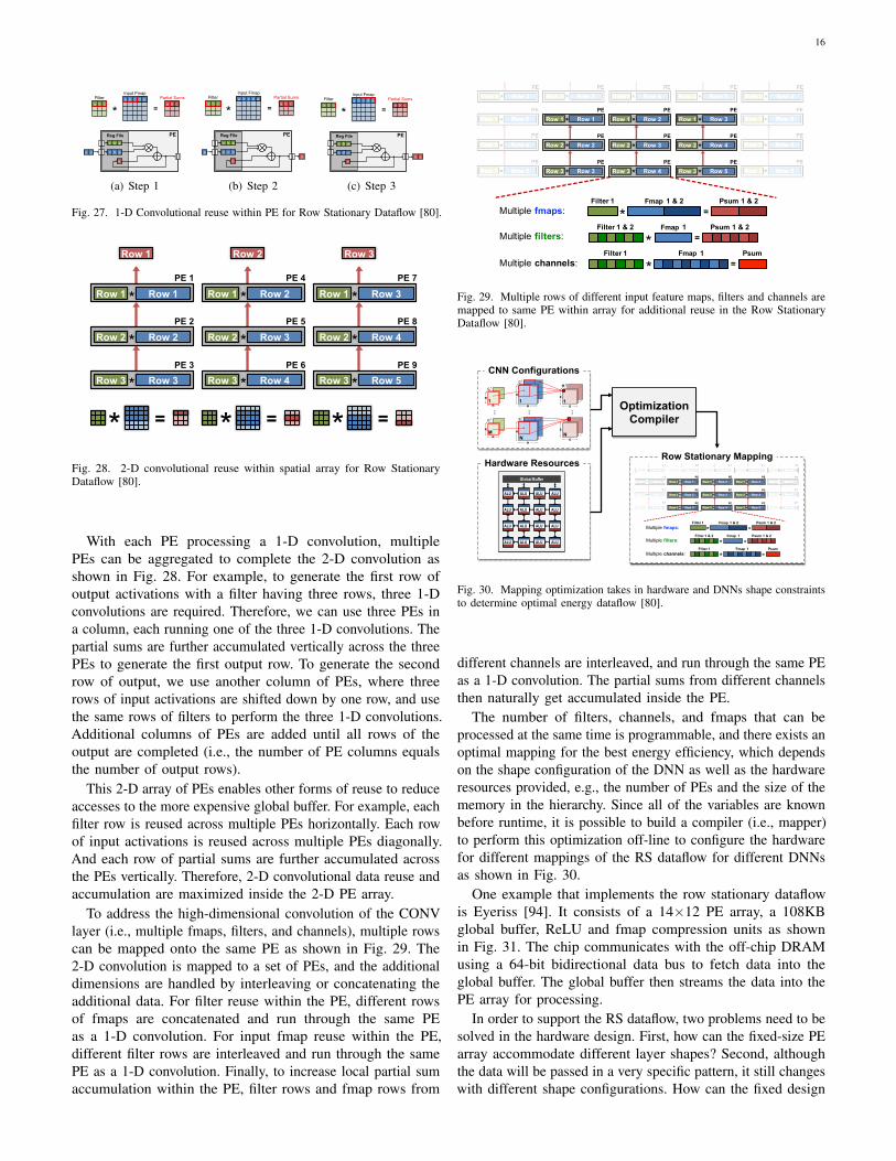
16

* = Filter a b c a b c

a b c d e

e d

PE b a c

Reg File

b a c

a

Partial Sums Input Fmap

(a) Step 1

* = a b c

a b c d e Partial Sums Input Fmap

PE b a c

Reg File

c b d

b

e a

Filter a b c

(b) Step 2

* = a b c

a b c d e Partial Sums Input Fmap

PE b a c

Reg File

d c e

c

b a

Filter a b c

(c) Step 3

Fig. 27. 1-D Convolutional reuse within PE for Row Stationary Dataflow [80].

PE 1

Row 1 Row 1

PE 2

Row 2 Row 2

PE 3

Row 3 Row 3

Row 1

= *

PE 4

Row 1 Row 2

PE 5

Row 2 Row 3

PE 6

Row 3 Row 4

Row 2

= *

PE 7

Row 1 Row 3

PE 8

Row 2 Row 4

PE 9

Row 3 Row 5

Row 3

= *

* * *

* * *

* * *

Fig. 28. 2-D convolutional reuse within spatial array for Row StationaryDataflow [80].

With each PE processing a 1-D convolution, multiplePEs can be aggregated to complete the 2-D convolution asshown in Fig. 28. For example, to generate the first row ofoutput activations with a filter having three rows, three 1-Dconvolutions are required. Therefore, we can use three PEs ina column, each running one of the three 1-D convolutions. Thepartial sums are further accumulated vertically across the threePEs to generate the first output row. To generate the secondrow of output, we use another column of PEs, where threerows of input activations are shifted down by one row, and usethe same rows of filters to perform the three 1-D convolutions.Additional columns of PEs are added until all rows of theoutput are completed (i.e., the number of PE columns equalsthe number of output rows).

This 2-D array of PEs enables other forms of reuse to reduceaccesses to the more expensive global buffer. For example, eachfilter row is reused across multiple PEs horizontally. Each rowof input activations is reused across multiple PEs diagonally.And each row of partial sums are further accumulated acrossthe PEs vertically. Therefore, 2-D convolutional data reuse andaccumulation are maximized inside the 2-D PE array.

To address the high-dimensional convolution of the CONVlayer (i.e., multiple fmaps, filters, and channels), multiple rowscan be mapped onto the same PE as shown in Fig. 29. The2-D convolution is mapped to a set of PEs, and the additionaldimensions are handled by interleaving or concatenating theadditional data. For filter reuse within the PE, different rowsof fmaps are concatenated and run through the same PEas a 1-D convolution. For input fmap reuse within the PE,different filter rows are interleaved and run through the samePE as a 1-D convolution. Finally, to increase local partial sumaccumulation within the PE, filter rows and fmap rows from

Multiple fmaps:

Multiple filters:

Multiple channels:

PERow 1 Row 1

PERow 2 Row 2

PERow 3 Row 3

PERow 1 Row 2

PERow 2 Row 3

PERow 3 Row 4

PERow 1 Row 3

PERow 2 Row 4

PERow 3 Row 5

* * *

* * *

* * *

Image 1=

PsumFilter 1

**

Image 1=

Psum 1 & 2Filter 1 & 2*

Image 1 & 2=

Psum 1 & 2Filter 1

Fmap

Fmap

Fmap

Fig. 29. Multiple rows of different input feature maps, filters and channels aremapped to same PE within array for additional reuse in the Row StationaryDataflow [80].

…

M

……

R

R

R

R

C

C

E

E

H

H

C

E

E1

N N

1

M

H

H

C

1

CNN Configurations

Global Buffer

ALU

ALU

ALU

ALU

ALU

ALU

ALU

ALU

ALU

ALU

ALU

ALU

ALU

ALU

ALU

ALU

Hardware Resources

Optimization Compiler

Row Stationary Mapping

Multiple fmaps:

Multiple filters:

Multiple channels:

PERow 1 Row 1

PERow 2 Row 2

PERow 3 Row 3

PERow 1 Row 2

PERow 2 Row 3

PERow 3 Row 4

PERow 1 Row 3

PERow 2 Row 4

PERow 3 Row 5

* * *

* * *

* * *

Image 1=

PsumFilter 1

**

Image 1=

Psum 1 & 2Filter 1 & 2*

Image 1 & 2=

Psum 1 & 2Filter 1

Fmap

Fmap

Fmap

Fig. 30. Mapping optimization takes in hardware and DNNs shape constraintsto determine optimal energy dataflow [80].

different channels are interleaved, and run through the same PEas a 1-D convolution. The partial sums from different channelsthen naturally get accumulated inside the PE.

The number of filters, channels, and fmaps that can beprocessed at the same time is programmable, and there exists anoptimal mapping for the best energy efficiency, which dependson the shape configuration of the DNN as well as the hardwareresources provided, e.g., the number of PEs and the size of thememory in the hierarchy. Since all of the variables are knownbefore runtime, it is possible to build a compiler (i.e., mapper)to perform this optimization off-line to configure the hardwarefor different mappings of the RS dataflow for different DNNsas shown in Fig. 30.

One example that implements the row stationary dataflowis Eyeriss [94]. It consists of a 14×12 PE array, a 108KBglobal buffer, ReLU and fmap compression units as shownin Fig. 31. The chip communicates with the off-chip DRAMusing a 64-bit bidirectional data bus to fetch data into theglobal buffer. The global buffer then streams the data into thePE array for processing.

In order to support the RS dataflow, two problems need to besolved in the hardware design. First, how can the fixed-size PEarray accommodate different layer shapes? Second, althoughthe data will be passed in a very specific pattern, it still changeswith different shape configurations. How can the fixed design

17

…

…

…

…

… …

RLCDecoder

Ifmap

Ofmap

Filter Filter

Ifmap

Psum

Psum

GlobalBuffer

108KB64 bits

Link Clock Core Clock Accelerator

RLCEnc.

Top-Level Control Config Scan ChainConfiguration Bits

MACSpad

Control

12✕14PE Array Processing

Element

Off-Chip DRAM

ReLU

Fig. 31. Eyeriss DNN accelerator [94].

Replication Folding

..

.. .. ..

..

.. 3

13 AlexNet Layer 3-5

12

14

Physical PE Array

3

3

3

3

13

13

13

13

..

.. .. ..

..

.. 5

27 AlexNet Layer 2

Physical PE Array

12

14

5 14

13 5

Unused PEs are

Clock Gated

Fig. 32. Mapping uses replication and folding to maximized utilization ofPE array [94].

pass data in different patterns?Two mapping strategies can be used to solve the first problem

as shown in Fig. 32. First, replication can be used to map shapesthat do not use up the entire PE array. For example, in thethird to fifth layers of AlexNet, each 2-D convolution only usesa 13×3 PE array. This structure is then replicated four times,and runs different channels and filters in each replication. Thesecond strategy is called folding. For example, in the secondlayer of AlexNet, it requires a 27×5 PE array to complete the2-D convolution. In order to fit it into the 14×12 physical PEarray, it is folded into two parts, 14×5 and 13×5, and eachare vertically mapped into the physical PE array. Since not allPEs are used by the mapping, the unused PEs can be clockgated to save energy consumption.

A custom multicast network is used to solve the secondproblem about flexible data delivery. The simplest way to passdata to multiple destinations is to broadcast the data to all PEsand let each PE decide if it has to process the data or not.However, it is not very energy efficient especially when thesize of PE array is large. Instead, a multicast network is usedto send data to only the places where it is needed.

5) Energy comparison of different dataflows: To evaluateand compare different dataflows, the same total hardware areaand number of PEs (256) are used in the simulation of a spatialarchitecture for all dataflows. The local memory (register file) ateach processing element (PE) is on the order of 0.5 – 1.0kB anda shared memory (global buffer) is on the order of 100 – 500kB.The sizes of these memories are selected to be comparable toa typical accelerator for multimedia processing, such as videocoding [95]. The memory sizes are further adjusted for the

needs of each dataflow under the same area constraint. Forexample, since the no local reuse dataflow does not require anyRF in PE, it is allocated with a much larger global buffer. Thesimulation uses the layer configurations from AlexNet with abatch size of 16. The simulation also takes into account thefact that accessing different levels of the memory hierarchyrequires different energy cost.

Fig. 33 compares the chip and DRAM energy consumptionof each dataflow for the CONV layers of AlexNet with abatch size of 16. The WS and OS dataflows have the lowestenergy consumption for accessing weights and partial sums,respectively. However, the RS dataflow has the lowest totalenergy consumption since it optimizes for the overall energyefficiency instead of only for a certain data type.

Fig. 33(a) shows the same results with breakdown in terms ofmemory hierarchy. The RS dataflow consumes the most energyin the RF, since by design most of the accesses have beenmoved to the lowest level of the memory hierarchy. This helpsto achieve the lowest total energy consumption since RF hasthe lowest energy per access. The NLR dataflow has the lowestenergy consumption at the DRAM level, since it has a muchlarger global buffer and thus higher on-chip storage capacitycompared to others. However, most of the data accesses inthe NLR dataflow is from the global buffer, which still has arelatively large energy consumption per access compared toaccessing data from RF or inside the PE array. As a result, theoverall energy consumption of the NLR dataflow is still fairlyhigh. Overall, RS dataflow uses 1.4× to 2.5× lower energythan other dataflows.

Fig. 34 shows the energy efficiency between differentdataflows in the FC layers of AlexNet with a batch size of 16.Since there is not as much data reuse in the FC layers as inthe CONV layers, all dataflows spend a significant amount ofenergy on reading weights. However, RS dataflow still has thelowest energy consumption because it optimizes for the energyof accessing input activations and partial sums. For the OSdataflows, OSC now consumes lower energy than OSA sinceit is designed for the FC layers. Overall, RS still consumes1.3× lower energy compared to other dataflows at the batchsize of 16.

Fig. 35 shows the RS dataflow design with energy breakdownin terms of different layers of AlexNet. In the CONV layers, theenergy is mostly consumed by the RF, while in the FC layers,the energy is mostly consumed by DRAM. However, mostof the energy is consumed by the CONV layers, which takesaround 80% of the energy. As recent DNN models go deeperwith more CONV layers, the ratio between number of CONVand FC layers only gets larger. Therefore, moving forward,significant effort should be placed on energy optimizations forCONV layers.

Finally, up until now, we have been looking at architec-tures with relatively limited storage on the order of a fewhundred kilobytes. With much larger storage on the order ofa few megabytes, additional dataflows can be considered. Forexample, Fused-Layer looks at dataflow optimizations acrosslayers [96].

18

NormalizedEnergy/MAC

RFNoC

bufferDRAMALU

WS OSA OSB OSC NLR RSDNN Dataflows

0

0.5

1

1.5

2

(a) Energy breakdown across memory hierarchy

0

0.5

1

1.5

2

NormalizedEnergy/MAC

WS OSA OSB OSC NLR RS

psums

weightspixels

DNN Dataflows

(b) Energy breakdown across data type

Fig. 33. Comparison of energy efficiency between different dataflows in theCONV layers of AlexNet with a batch size of 16 [3]: (a) breakdown in termsof storage levels and ALU, (b) breakdown in terms of data types. OSA, OSB

and OSC are three variants of the OS dataflow that are commonly seen indifferent implementations [80].

0

0.5

1

1.5

2

psums

weightspixels

NormalizedEnergy/MAC

WS OSA OSB OSC NLR RSDNN Dataflows

Fig. 34. Comparison of energy efficiency between different dataflows in theFC layers of AlexNet with a batch size of 16 [80].

VI. NEAR-DATA PROCESSING

The previous section highlighted that data movement domi-nates energy consumption. While spatial architectures distributethe on-chip memory such that it is closer to the computation(e.g., into the PE), there have also been efforts to bring theoff-chip high density memory closer to the computation or tointegrate the computation into the memory itself; the latter isoften referred to as processing-in-memory or logic-in-memory.In embedded systems, there have also been efforts to bring thecomputation into the sensor where the data is first collected.

ALU

RF

NoC

buffer

DRAM

2.0e10

1.5e10

1.0e10

0.5e10

0L1 L8 L2 L3 L4 L5 L6 L7

Normalized Energy

(1 MAC = 1)

CONV Layers FC Layers

RF dominates DRAM dominates

Total Energy 80% 20%

Fig. 35. Energy breakdown across layers of the AlexNet [80]. RF energydominates in convolutional layers. DRAM energy dominates in the fullyconnected layer. Convolutional layer dominate energy consumption.

In this section, we will discuss how moving compute and datacloser to reduce data movement (i.e., near-data processing) canbe achieved using mixed-signal circuit design and advancedmemory technologies.

Many of these works use analog processing which has thedrawback of increased sensitivity to circuit and device non-idealities. Consequentially, the computation is often performedat reduced precision, which can be accounted for duringthe training of the DNNs using the techniques discussed inSection VII. Another factor to take into consideration is thatDNNs are often trained in the digital domain; thus for analogprocessing, there is an additional overhead cost for analog-to-digital conversion (ADC) and digital-to-analog conversion(DAC).

A. DRAM

Advanced memory technology can reduce the access energyfor high density memories such as DRAMs. For instance,embedded DRAM (eDRAM) brings high density memory on-chip to avoid the high energy cost of switching off-chipcapacitance [97]; eDRAM is 2.85× higher density than SRAMand 321× more energy efficient than DRAM (DDR3) [93].eDRAM also offers higher bandwidth and lower latencycompared to DRAM. In DNN processing, eDRAM can be usedto store tens of megabytes of weights and activations on-chipto avoid off-chip access, as demonstrated in DaDianNao [93].The downside of eDRAM is that it has lower density thanoff-chip DRAM and can increase the cost of the chip.

Rather than integrating DRAM into the chip itself, theDRAM can also be stacked on top of the chip using throughsilicon vias (TSV). This technology is often referred to as 3-Dmemory, and has been commercialized in the form of HybridMemory Cube (HMC) [98] and High Bandwidth Memory(HBM) [99]. 3-D memory delivers an order of magnitude higherbandwidth and reduces access energy by up to 5× relative toexisting 2-D DRAMs, as TSV have lower capacitance thantypical off-chip interconnects. Recent works have explored theuse of HMC for efficient DNN processing in a variety of ways.For instance, Neurocube [100] integrates SIMD processors intothe logic die of the HMC to bring the memory and computation

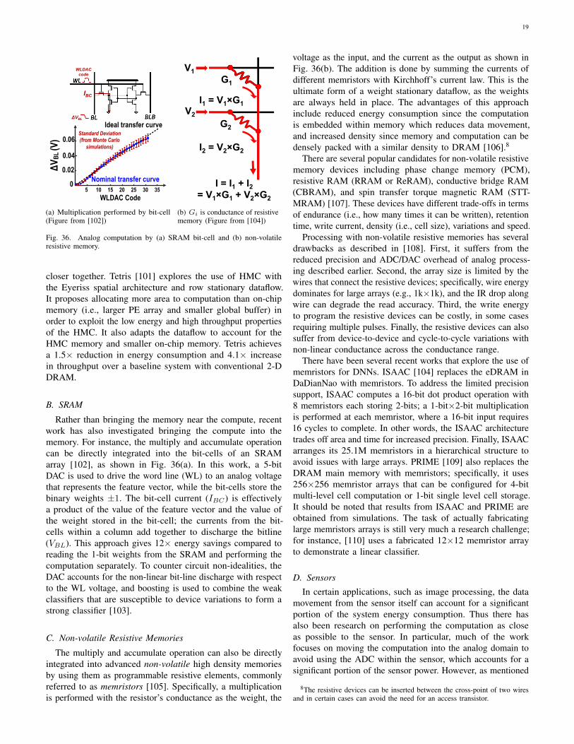
19

0.02

0.04

0.06

WLDAC Code

ΔVBL

(V)

05 10 15 20 25 30 35

Ideal transfer curve

Nominal transfer curve

Standard Deviation (from Monte Carlo

simulations)

IBC

WLDAC code

ΔVBL

(a) Multiplication performed by bit-cell(Figure from [102])

V1 G1

I1 = V1×G1 V2

G2

I2 = V2×G2

I = I1 + I2 = V1×G1 + V2×G2

(b) Gi is conductance of resistivememory (Figure from [104])

Fig. 36. Analog computation by (a) SRAM bit-cell and (b) non-volatileresistive memory.

closer together. Tetris [101] explores the use of HMC withthe Eyeriss spatial architecture and row stationary dataflow.It proposes allocating more area to computation than on-chipmemory (i.e., larger PE array and smaller global buffer) inorder to exploit the low energy and high throughput propertiesof the HMC. It also adapts the dataflow to account for theHMC memory and smaller on-chip memory. Tetris achievesa 1.5× reduction in energy consumption and 4.1× increasein throughput over a baseline system with conventional 2-DDRAM.

B. SRAM

Rather than bringing the memory near the compute, recentwork has also investigated bringing the compute into thememory. For instance, the multiply and accumulate operationcan be directly integrated into the bit-cells of an SRAMarray [102], as shown in Fig. 36(a). In this work, a 5-bitDAC is used to drive the word line (WL) to an analog voltagethat represents the feature vector, while the bit-cells store thebinary weights ±1. The bit-cell current (IBC) is effectivelya product of the value of the feature vector and the value ofthe weight stored in the bit-cell; the currents from the bit-cells within a column add together to discharge the bitline(VBL). This approach gives 12× energy savings compared toreading the 1-bit weights from the SRAM and performing thecomputation separately. To counter circuit non-idealities, theDAC accounts for the non-linear bit-line discharge with respectto the WL voltage, and boosting is used to combine the weakclassifiers that are susceptible to device variations to form astrong classifier [103].

C. Non-volatile Resistive Memories

The multiply and accumulate operation can also be directlyintegrated into advanced non-volatile high density memoriesby using them as programmable resistive elements, commonlyreferred to as memristors [105]. Specifically, a multiplicationis performed with the resistor’s conductance as the weight, the

voltage as the input, and the current as the output as shown inFig. 36(b). The addition is done by summing the currents ofdifferent memristors with Kirchhoff’s current law. This is theultimate form of a weight stationary dataflow, as the weightsare always held in place. The advantages of this approachinclude reduced energy consumption since the computationis embedded within memory which reduces data movement,and increased density since memory and computation can bedensely packed with a similar density to DRAM [106].8

There are several popular candidates for non-volatile resistivememory devices including phase change memory (PCM),resistive RAM (RRAM or ReRAM), conductive bridge RAM(CBRAM), and spin transfer torque magnetic RAM (STT-MRAM) [107]. These devices have different trade-offs in termsof endurance (i.e., how many times it can be written), retentiontime, write current, density (i.e., cell size), variations and speed.

Processing with non-volatile resistive memories has severaldrawbacks as described in [108]. First, it suffers from thereduced precision and ADC/DAC overhead of analog process-ing described earlier. Second, the array size is limited by thewires that connect the resistive devices; specifically, wire energydominates for large arrays (e.g., 1k×1k), and the IR drop alongwire can degrade the read accuracy. Third, the write energyto program the resistive devices can be costly, in some casesrequiring multiple pulses. Finally, the resistive devices can alsosuffer from device-to-device and cycle-to-cycle variations withnon-linear conductance across the conductance range.

There have been several recent works that explore the use ofmemristors for DNNs. ISAAC [104] replaces the eDRAM inDaDianNao with memristors. To address the limited precisionsupport, ISAAC computes a 16-bit dot product operation with8 memristors each storing 2-bits; a 1-bit×2-bit multiplicationis performed at each memristor, where a 16-bit input requires16 cycles to complete. In other words, the ISAAC architecturetrades off area and time for increased precision. Finally, ISAACarranges its 25.1M memristors in a hierarchical structure toavoid issues with large arrays. PRIME [109] also replaces theDRAM main memory with memristors; specifically, it uses256×256 memristor arrays that can be configured for 4-bitmulti-level cell computation or 1-bit single level cell storage.It should be noted that results from ISAAC and PRIME areobtained from simulations. The task of actually fabricatinglarge memristors arrays is still very much a research challenge;for instance, [110] uses a fabricated 12×12 memristor arrayto demonstrate a linear classifier.

D. Sensors

In certain applications, such as image processing, the datamovement from the sensor itself can account for a significantportion of the system energy consumption. Thus there hasalso been research on performing the computation as closeas possible to the sensor. In particular, much of the workfocuses on moving the computation into the analog domain toavoid using the ADC within the sensor, which accounts for asignificant portion of the sensor power. However, as mentioned

8The resistive devices can be inserted between the cross-point of two wiresand in certain cases can avoid the need for an access transistor.

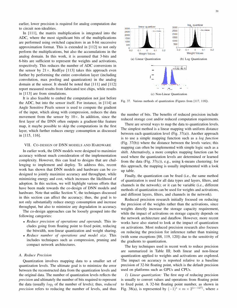
20

earlier, lower precision is required for analog computation dueto circuit non-idealities.

In [111], the matrix multiplication is integrated into theADC, where the most significant bits of the multiplicationsare performed using switched capacitors in an 8-bit successiveapproximation format. This is extended in [112] to not onlyperform the multiplications, but also the accumulations in theanalog domain. In this work, it is assumed that 3-bits and6-bits are sufficient to represent the weights and activations,respectively. This reduces the number of ADC conversions inthe sensor by 21×. RedEye [113] takes this approach evenfurther by performing the entire convolution layer (includingconvolution, max pooling and quantization) in the analogdomain at the sensor. It should be noted that [111] and [112]report measured results from fabricated test chips, while resultsin [113] are from simulations.

It is also feasible to embed the computation not just beforethe ADC, but into the sensor itself. For instance, in [114] anAngle Sensitive Pixels sensor is used to compute the gradientof the input, which along with compression, reduces the datamovement from the sensor by 10×. In addition, since thefirst layer of the DNN often outputs a gradient-like featuremap, it maybe possible to skip the computations in the firstlayer, which further reduces energy consumption as discussedin [115, 116].

VII. CO-DESIGN OF DNN MODELS AND HARDWARE

In earlier work, the DNN models were designed to maximizeaccuracy without much consideration of the implementationcomplexity. However, this can lead to designs that are chal-lenging to implement and deploy. To address this, recentwork has shown that DNN models and hardware can be co-designed to jointly maximize accuracy and throughput, whileminimizing energy and cost, which increases the likelihood ofadoption. In this section, we will highlight various efforts thathave been made towards the co-design of DNN models andhardware. Note that unlike Section V, the techniques discussedin this section can affect the accuracy; thus, the goal is tonot only substantially reduce energy consumption and increasethroughput, but also to minimize any degradation in accuracy.

The co-design approaches can be loosely grouped into thefollowing categories:

• Reduce precision of operations and operands. This in-cludes going from floating point to fixed point, reducingthe bitwidth, non-linear quantization and weight sharing.

• Reduce number of operations and model size. Thisincludes techniques such as compression, pruning andcompact network architectures.

A. Reduce Precision

Quantization involves mapping data to a smaller set ofquantization levels. The ultimate goal is to minimize the errorbetween the reconstructed data from the quantization levels andthe original data. The number of quantization levels reflects theprecision and ultimately the number of bits required to representthe data (usually log2 of the number of levels); thus, reducedprecision refers to reducing the number of levels, and thus

(a) Linear Quantization (b) Log Quantization

(c) Non-Linear Quantization

Fig. 37. Various methods of quantization (Figures from [117, 118]).

the number of bits. The benefits of reduced precision includereduced storage cost and/or reduced computation requirements.

There are several ways to map the data to quantization levels.The simplest method is a linear mapping with uniform distancebetween each quantization level (Fig. 37(a)). Another approachis to use a simple mapping function such as a log function(Fig. 37(b)) where the distance between the levels varies; thismapping can often be implemented with simple logic such as ashift. Alternatively, a more complex mapping function can beused where the quantization levels are determined or learnedfrom the data (Fig. 37(c)), e.g., using k-means clustering; forthis approach, the mapping is usually implemented with a lookup table.

Finally, the quantization can be fixed (i.e., the same methodof quantization is used for all data types and layers, filters, andchannels in the network); or it can be variable (i.e., differentmethods of quantization can be used for weights and activations,and different layers, filters, and channels in the network).

Reduced precision research initially focused on reducingthe precision of the weights rather than the activations, sinceweights directly increase the storage capacity requirement,while the impact of activations on storage capacity depends onthe network architecture and dataflow. However, more recentworks have also started to look at the impact of quantizationon activations. Most reduced precision research also focuseson reducing the precision for inference rather than training(with some exceptions [88, 119, 120]) due to the sensitivity ofthe gradients to quantization.

The key techniques used in recent work to reduce precisionare summarized in Table III; both linear and non-linearquantization applied to weights and activations are explored.The impact on accuracy is reported relative to a baselineprecision of 32-bit floating point, which is the default precisionused on platforms such as GPUs and CPUs.

1) Linear quantization: The first step of reducing precisionis usually to convert values and operations from floating pointto fixed point. A 32-bit floating point number, as shown inFig. 38(a), is represented by (−1)s ×m× 2(e−127), where s

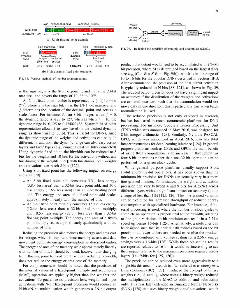
21

1 0 1 0 0 1 0 1 0 0 0 0 0 0 0 0 0 1 0 1 0 0 0 0 0 0 0 0 0 1 0 0 32-bit float

exponent (8-bits) mantissa (23-bits) sign

e = 70 s = 1 m = 20482 -1.42122425 x 10-13

(a) 32-bit floating point example

1 0 1 0 0 1 0 1 0 0 0 0 0 0 0 0 0 1 0 1 0 0 0 0 0 0 0 0 0 1 0 032-bit float

exponent (8-bits) mantissa (23-bits)sign

8-bit

dynamic

fixed

0 1 1 0 0 1 1 0

sign

integer

([7-f ]-bits)

mantissa (7-bits)

fractional

(f-bits)

e = 70s = 1 m = 20482-1.42122425 x 10-13

f = 3s = 012.75 m=102

8-bit

dynamic

fixed

0 1 1 0 0 1 1 0

sign mantissa (7-bits)

fractional

(f-bits)

f = 9s = 00.19921875 m=102

(b) 8-bit dynamic fixed point examples

Fig. 38. Various methods of number representations.

is the sign bit, e is the 8-bit exponent, and m is the 23-bitmantissa, and covers the range of 10−38 to 1038.

An N-bit fixed point number is represented by (−1)s×m×2−f , where s is the sign bit, m is the (N-1)-bit mantissa, andf determines the location of the decimal point and acts as ascale factor. For instance, for an 8-bit integer, when f = 0,the dynamic range is -128 to 127, whereas when f = 10, thedynamic range is -0.125 to 0.124023438. Dynamic fixed pointrepresentation allows f to vary based on the desired dynamicrange as shown in Fig. 38(b). This is useful for DNNs, sincethe dynamic range of the weights and activations can be quitedifferent. In addition, the dynamic range can also vary acrosslayers and layer types (e.g., convolutional vs. fully connected).Using dynamic fixed point, the bitwidth can be reduced to 8bits for the weights and 10 bits for the activations without anyfine-tuning of the weights [121]; with fine-tuning, both weightsand activations can reach 8-bits [122].

Using 8-bit fixed point has the following impact on energyand area [79]:

• An 8-bit fixed point add consumes 3.3× less energy(3.8× less area) than a 32-bit fixed point add, and 30×less energy (116× less area) than a 32-bit floating pointadd. The energy and area of a fixed-point add scalesapproximately linearly with the number of bits.

• An 8-bit fixed point multiply consumes 15.5× less energy(12.4× less area) than a 32-bit fixed point multiply,and 18.5× less energy (27.5× less area) than a 32-bitfloating point multiply. The energy and area of a fixed-point multiply scales approximately quadratically with thenumber of bits.

Reducing the precision also reduces the energy and area costfor storage, which is important since memory access and datamovement dominate energy consumption as described earlier.The energy and area of the memory scale approximately linearlywith number of bits. It should be noted, however, that changingfrom floating point to fixed point, without reducing bit-width,does not reduce the energy or area cost of the memory.

For completeness, it should be noted that the precision ofthe internal values of a fixed-point multiply and accumulate(MAC) operation are typically higher than the weights andactivations. To guarantee no precision loss, weights and inputactivations with N-bit fixed-point precision would require anN-bit×N-bit multiplication which generates a 2N-bit output

Accumulate +

Weight (N-bits)

Activation (N-bits)

N x N multiply

2N-bits

2N+M-bits

Output (N-bits)

Quantize to N-bits

Fig. 39. Reducing the precision of multiply and accumulate (MAC).

product; that output would need to be accumulated with 2N+M-bit precision, where M is determined based on the largest filtersize log2(C ×R× S from Fig. 9(b)), which is in the range of10 to 16 bits for the popular DNNs described in Section III-B.After accumulation, the precision of the final output activationis typically reduced to N-bits [88, 121], as shown in Fig. 39.The reduced output precision does not have a significant impacton accuracy if the distribution of the weights and activationsare centered near zero such that the accumulation would notmove only in one direction; this is particularly true when batchnormalization is used.

The reduced precision is not only explored in research,but has been used in recent commercial platforms for DNNprocessing. For instance, Google’s Tensor Processing Unit(TPU) which was announced in May 2016, was designed for8-bit integer arithmetic [123]. Similarly, Nvidia’s PASCALGPU, which was announced in April 2016, also has 8-bitinteger instructions for deep learning inference [124]. In generalpurpose platforms such as CPUs and GPUs, the main benefitof using 8-bit computation is an increase in throughput, asfour 8-bit operations rather than one 32-bit operation can beperformed for a given clock cycle.

While general purpose platforms usually support 8-bit,16-bit and/or 32-bit operations, it has been shown that theminimum bit precision for DNNs can actually vary in a morefine grained manner. For instance, the weight and activationprecision can vary between 4 and 9 bits for AlexNet acrossdifferent layers without significant impact on accuracy (i.e., achange of less than 1%) [125, 126]. This fine-grained variationcan be exploited for increased throughput or reduced energyconsumption with specialized hardware. For instance, if bit-serial processing is used, where the number of clock cycles tocomplete an operation is proportional to the bitwidth, adaptingto fine-grain variations in bit precision can result in a 2.24×speed up versus 16-bits [125]. Alternatively, a multiplier canbe designed such that its critical path reduces based on the bitprecision as fewer adders are needed to resolve the product;this can be combined with voltage scaling for a 2.56× energysavings versus 16-bits [126]. While these bit scaling resultsare reported relative to 16-bit, it would be interesting to seetheir impact relative to the maximum precision required acrosslayers (i.e., 9-bits for [125, 126]).

The precision can be reduced even more aggressively to asingle bit; this area of research is often referred to as binary nets.BinaryConnect (BC) [127] introduced the concept of binaryweights (i.e., -1 and 1), where using a binary weight reducedthe multiplication in the MAC to addition and subtractiononly. This was later extended in Binarized Neural Networks(BNN) [128] that uses binary weights and activations, which

22

reduces the MAC to an XNOR. However, BC and BNN havean accuracy loss of 19% and 29.8%, respectively [129].

In order to reduce this accuracy loss, Binary WeightNets (BWN) and XNOR-Nets introduced several significantmodifications to the DNN processing [129]. This includesmultiplying the outputs with a scale factor to recover thedynamic range (i.e., the weights effectively become -w andw, where w is the average of the absolute values of theweights in the filter)9, keeping the first and last layers at 32-bitfloating point precision, and performing normalization beforeconvolution to reduce the dynamic range of the activations.With these changes, BWN reduced the accuracy loss to 0.8%,while XNOR-Nets reduced the loss to 11%. The loss of XNOR-Net can be further reduced by increasing the precision of theactivations to be slightly larger than one bit. For instance,Quantized Neural Networks (QNN) [119], DoReFa-Net [120],and HWGQ-Net [130] allow the activations to have 2-bits,while the weights remain at 1-bit; in HWGQ-Net, this reducesthe accuracy loss to 5.2%.

All the previously described binary nets limit the weightsto two values (-w and w); however, there may be benefitsfor allowing weights to be zero (i.e., -w, 0, w). Althoughthis requires an additional bit per weight compared to binaryweights, the sparsity of the weights can be exploited to reducecomputation and storage cost, which can potentially cancelout the cost of the additional bit. This is explored in TernaryWeight Nets (TWN) [131] and then extended in Trained TernaryQuantization (TTQ) where a different scale is trained for eachweight (i.e., -w1, 0, w2) for an accuracy loss of 0.6% [132],assuming 32-bit floating point for the activations.

Hardware implementations for binary/ternary nets havebeen explored in recent publications. YodaNN [133] usesbinary weights, while BRein [134] uses binary weights andactivations. Binary weights are also used in the computein SRAM work [102] described in Section VI. Finally, thenominally spike-inspired TrueNorth chip can implement areduced precision neural network with binary activations andternary weights using TrueNorth’s quantized weight table [9].These works tend not to support state-of-the-art DNN models(with the exception of YodaNN).

2) Non-linear quantization: The previous works describedinvolve linear quantization where the levels are uniformlyspaced out. It has been shown that the distributions of theweights and activations are not uniform [118, 135], and thusa non-linear quantization can potentially improve accuracy.Specifically, there have been two popular approaches takenin recent works: (1) log domain quantization; (2) learnedquantization or weight sharing.

Log domain quantization If the quantization levels areassigned based on a logarithmic distribution as shown inFig 37(b), the weights and activations are more equallydistributed across the different levels and each level is usedmore efficiently resulting in less quantization error. For instance,using 4 bits in linear quantization results in a 27.8% loss inaccuracy versus a 5% loss for log base-2 quantization for

9This can also be thought of as a form of weights sharing, where only twoweights are used per filter.

Weight Decoder/Dequant U x 16b

Weight index

(log2U-bits) Weight

(16-bits) Weight Memory CRSM x

log2U-bits Output

Activation (16-bits)

MAC

Input Activation (16-bits)

Fig. 40. Weight sharing hardware.

VGG-16 [117]. Furthermore, when weights are quantized topowers of two, the multiplication can be replaced with a bit-shift [122, 135].10 Incremental Network Quantization (INQ)can be used to further reduce the loss in accuracy by dividingthe large and small weights into different groups, and theniteratively quantizing and re-training the weights [136].

Weight Sharing forces several weights to share a single value.This reduces the number of unique weights in a filter or alayer. One example is to group the weights by using a hashingfunction and use one value for each group [137]. Alternatively,the weights can be grouped by the k-means algorithm [118].Both the shared weights and the indexes indicating whichweight to use at each position of the filter are stored. Thisleads to a two step process to fetch the weight: (1) read theweight index; (2) using the weight index, read the sharedweights. This approach can reduce the cost of reading andstoring the weights if the weight index (log2 of the number ofunique weights) is less than the bitwidth of the weight itself.

For instance, in Deep Compression [118], the number ofunique weights per layer is reduced to 256 for convolutionallayers and 16 for fully-connected layers in AlexNet, requiring8-bit and 4-bit weight indexes, respectively. Assuming thereare U unique weights and the size of the filters in the layeris C×R×S×M from Fig. 9(b), there will be energy savingsif reading from a CRSM × log2U -bit memory plus a U×16-bit memory (as shown in Fig. 40) cost less than readingfrom a CRSM×16-bit memory. Note that unlike the previousquantization methods, the weight sharing approach does notreduce the precision of the MAC computation itself and onlyreduces the weight storage requirement.

B. Reduce Number of Operations and Model Size

In addition to reducing the size of each operation or operand(weight/activation), there is also a significant amount of researchon methods to reduce the number of operations and modelsize. These techniques can be loosely classified as exploitingactivation statistics, network pruning, network architecturedesign and knowledge distillation.

1) Exploiting Activation Statistics: As discussed in Sec-tion III-A1, ReLU is a popular form of non-linearity used inDNNs that sets all negative values to zero as shown in Fig. 41(a).As a result, the output activations of the feature maps after theReLU are sparse; for instance, the feature maps in AlexNethave sparsity between 19% to 63% as shown in Fig. 41(b).This sparsity gives ReLU an implementation advantage overother non-linearities such as sigmoid, etc.

10Note however that multiplications do not account for a significant portionof the total energy.

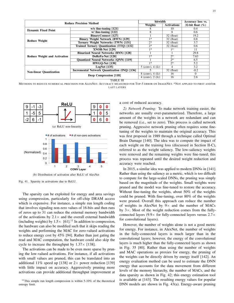
23

Reduce Precision Method bitwidth Accuracy loss vs.Weights Activations 32-bit float (%)

Dynamic Fixed Point w/o fine-tuning [121] 8 10 0.4w/ fine-tuning [122] 8 8 0.6

Reduce Weight

BinaryConnect [127] 1 32 (float) 19.2Binary Weight Network (BWN) [129] 1* 32 (float) 0.8

Ternary Weight Networks (TWN) [131] 2* 32 (float) 3.7Trained Ternary Quantization (TTQ) [132] 2* 32 (float) 0.6

Reduce Weight and Activation

XNOR-Net [129] 1* 1* 11Binarized Neural Networks (BNN) [128] 1 1 29.8

DoReFa-Net [120] 1* 2* 7.63Quantized Neural Networks (QNN) [119] 1 2* 6.5

HWGQ-Net [130] 1* 2* 5.2

Non-linear Quantization

LogNet [135] 5 (conv), 4 (fc) 4 3.2Incremental Network Quantization (INQ) [136] 5 32 (float) -0.2

Deep Compression [118] 8 (conv), 4 (fc) 16 04 (conv), 2 (fc) 16 2.6

TABLE IIIMETHODS TO REDUCE NUMERICAL PRECISION FOR ALEXNET. ACCURACY MEASURED FOR TOP-5 ERROR ON IMAGENET. *NOT APPLIED TO FIRST AND/OR

LAST LAYERS

9 -1 -3 1 -5 5 -2 6 -1

ReLU 9 0 0 1 0 5 0 6 0

(a) ReLU non-linearity

0

0.2

0.4

0.6

0.8

1

1 2 3 4 5 CONV Layer

# of activations # of non-zero activations

(Normalized)

(b) Distribution of activation after ReLU of AlexNet

Fig. 41. Sparsity in activations due to ReLU.

The sparsity can be exploited for energy and area savingsusing compression, particularly for off-chip DRAM accesswhich is expensive. For instance, a simple run length codingthat involves signaling non-zero values of 16-bits and then runsof zeros up to 31 can reduce the external memory bandwidthof the activations by 2.1× and the overall external bandwidth(including weights) by 1.5× [61].11 In addition to compression,the hardware can also be modified such that it skips reading theweights and performing the MAC for zero-valued activationsto reduce energy cost by 45% [94]. Rather than just gating theread and MAC computation, the hardware could also skip thecycle to increase the throughput by 1.37× [138].

The activations can be made to be even more sparse by prun-ing the low-valued activations. For instance, if all activationswith small values are pruned, this can be translated into anadditional 11% speed up [138] or 2× power reduction [139]with little impact on accuracy. Aggressively pruning moreactivations can provide additional throughput improvement at

11This simple run length compression is within 5-10% of the theoreticalentropy limit.

a cost of reduced accuracy.

2) Network Pruning: To make network training easier, thenetworks are usually over-parameterized. Therefore, a largeamount of the weights in a network are redundant and canbe removed (i.e., set to zero). This process is called networkpruning. Aggressive network pruning often requires some fine-tuning of the weights to maintain the original accuracy. Thiswas first proposed in 1989 through a technique called OptimalBrain Damage [140]. The idea was to compute the impact ofeach weight on the training loss (discussed in Section II-C),referred to as the weight saliency. The low-saliency weightswere removed and the remaining weights were fine-tuned; thisprocess was repeated until the desired weight reduction andaccuracy were reached.

In 2015, a similar idea was applied to modern DNNs in [141].Rather than using the saliency as a metric, which is too difficultto compute for the large-scaled DNNs, the pruning was simplybased on the magnitude of the weights. Small weights werepruned and the model was fine-tuned to restore the accuracy.Without fine-tuning the weights, about 50% of the weightscould be pruned. With fine-tuning, over 80% of the weightswere pruned. Overall this approach can reduce the numberof weights in AlexNet by 9× and the number of MACsby 3×. Most of the weight reduction comes from the fully-connected layers (9.9× for fully-connected layers versus 2.7×for convolutional layers).

However, the number of weights alone is not a good metricfor energy. For instance, in AlexNet, the number of weightsin the fully-connected layers is much larger than in theconvolutional layers; however, the energy of the convolutionallayers is much higher than the fully-connected layers as shownin Fig. 35 [80]. Rather than using the number of weightsand MAC operations as proxies for energy, the pruning ofthe weights can be directly driven by energy itself [142]. Anenergy evaluation method can be used to estimate the DNNenergy that accounts for the data movement from differentlevels of the memory hierarchy, the number of MACs, and thedata sparsity as shown in Fig. 42; this energy estimation toolis available at [143]. The resulting energy values for popularDNN models are shown in Fig. 43(a). Energy-aware pruning

24

CNN Shape Configuration (# of channels, # of filters, etc.)

CNN Weights and Input Data

[0.3, 0, -0.4, 0.7, 0, 0, 0.1, …]

CNN Energy Consumption L1 L2 L3

Energy

…

Memory Accesses

Optimization

# of MACs Calculation

…

# acc. at mem. level 1 # acc. at mem. level 2

# acc. at mem. level n

# of MACs

Hardware Energy Costs of each MAC and Memory Access

Ecomp

Edata

Fig. 42. Energy estimation methodology from [142], which estimates theenergy based on data movement from different levels of the memory hierarchy,number of MACs, and data sparsity.

AlexNet SqueezeNet

GoogLeNet

ResNet-50VGG-16

77%

79%

81%

83%

85%

87%

89%

91%

93%

5E+08 5E+09 5E+10

Top-5Ac

curacy

NormalizedEnergyConsump9on

OriginalDNN

(a) Energy versus accuracy trade-off of popular DNN models.

AlexNet SqueezeNet

GoogLeNet

ResNet-50VGG-16

AlexNet

SqueezeNet

AlexNet SqueezeNet

GoogLeNet

77%

79%

81%

83%

85%

87%

89%

91%

93%

5E+08 5E+09 5E+10

Top-5Ac

curacy

NormalizedEnergyConsump9on

OriginalDNN Magnitude-basedPruning Energy-awarePruning

1.74x

(b) Impact of energy-aware pruning.

Fig. 43. Energy values estimated with methodology in [142].

can then be used to prune weights based on energy to reducethe overall energy across all layers by 3.7× for AlexNet, whichis 1.74× more efficient than magnitude-based approaches [141]as shown in Fig. 43(b). As mentioned previously, it is wellknown that AlexNet is over-parameterized. The energy-awarepruning can also be applied to GoogleNet, which is already asmall DNN model, for a 1.6× energy reduction.

Recent works have examine how to efficiently supportprocessing of sparse weights in hardware. One area of interestis how to best store the sparse weights after pruning. Similar tocompressing the sparse activations discussed in Section VII-B1,the sparse weights can be compressed to reduce memory accessbandwidth by 20 to 30% [118].

When DNN processing is performed as a matrix-vector

# of filters

# of weights

(a) Compressed sparse row (CSR)

(b) Compressed sparse column (CSC)

Fig. 44. Sparse matrix-vector multiplications using different storage formats(Figure from [144]).

multiplication, as shown in Fig. 18(a), one challenge isto determine how to store the sparse weight matrix in acompressed format. The compression can be applied eitherin row or column order. A compressed sparse row (CSR)format, as shown in Fig. 44(a), is often used to perform SparseMatrix-Vector multiplication. However, the input vector needsto be read in multiple times even though only a subset of it isused since each row of the matrix is sparse. Alternatively,a compressed sparse column (CSC) format, as shown inFig. 44(b), can be used, where the output is updated severaltimes, and only one element of the input vector is read ata time [144]. The CSC format will provide an overall lowermemory bandwidth than CSR if the output is smaller than theinput, or in the case of DNN, if the number of filters is notsignificantly larger than the number of weights in the filter(C ×R× S from Fig. 9(b)). Since this is often true, CSC canbe an effective format for sparse DNN processing.

Custom hardware has been explored to efficiently supportpruned DNN models. Many works aim to perform the process-ing without decompressing the weights or activations. EIE [145]performs the sparse matrix-vector multiplication specifically forthe fully connected layers. It stores the weights in a CSC formatalong with the start location of each column, which needs to bestored since the compressed weights have variable length. Whenthe input is not zero, the compressed weight column is read andthe output is updated. To handle the sparsity, additional logicis used to keep track of the location of the output that shouldbe updated. SCNN [146] supports processing of convolutional

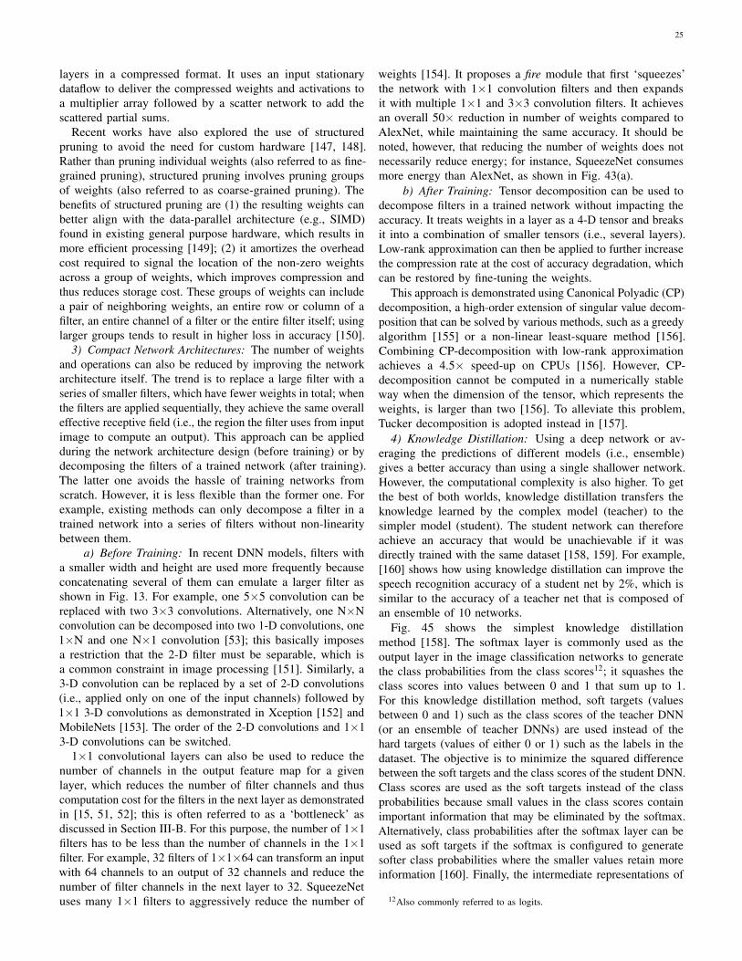
25

layers in a compressed format. It uses an input stationarydataflow to deliver the compressed weights and activations toa multiplier array followed by a scatter network to add thescattered partial sums.

Recent works have also explored the use of structuredpruning to avoid the need for custom hardware [147, 148].Rather than pruning individual weights (also referred to as fine-grained pruning), structured pruning involves pruning groupsof weights (also referred to as coarse-grained pruning). Thebenefits of structured pruning are (1) the resulting weights canbetter align with the data-parallel architecture (e.g., SIMD)found in existing general purpose hardware, which results inmore efficient processing [149]; (2) it amortizes the overheadcost required to signal the location of the non-zero weightsacross a group of weights, which improves compression andthus reduces storage cost. These groups of weights can includea pair of neighboring weights, an entire row or column of afilter, an entire channel of a filter or the entire filter itself; usinglarger groups tends to result in higher loss in accuracy [150].

3) Compact Network Architectures: The number of weightsand operations can also be reduced by improving the networkarchitecture itself. The trend is to replace a large filter with aseries of smaller filters, which have fewer weights in total; whenthe filters are applied sequentially, they achieve the same overalleffective receptive field (i.e., the region the filter uses from inputimage to compute an output). This approach can be appliedduring the network architecture design (before training) or bydecomposing the filters of a trained network (after training).The latter one avoids the hassle of training networks fromscratch. However, it is less flexible than the former one. Forexample, existing methods can only decompose a filter in atrained network into a series of filters without non-linearitybetween them.

a) Before Training: In recent DNN models, filters witha smaller width and height are used more frequently becauseconcatenating several of them can emulate a larger filter asshown in Fig. 13. For example, one 5×5 convolution can bereplaced with two 3×3 convolutions. Alternatively, one N×Nconvolution can be decomposed into two 1-D convolutions, one1×N and one N×1 convolution [53]; this basically imposesa restriction that the 2-D filter must be separable, which isa common constraint in image processing [151]. Similarly, a3-D convolution can be replaced by a set of 2-D convolutions(i.e., applied only on one of the input channels) followed by1×1 3-D convolutions as demonstrated in Xception [152] andMobileNets [153]. The order of the 2-D convolutions and 1×13-D convolutions can be switched.

1×1 convolutional layers can also be used to reduce thenumber of channels in the output feature map for a givenlayer, which reduces the number of filter channels and thuscomputation cost for the filters in the next layer as demonstratedin [15, 51, 52]; this is often referred to as a ‘bottleneck’ asdiscussed in Section III-B. For this purpose, the number of 1×1filters has to be less than the number of channels in the 1×1filter. For example, 32 filters of 1×1×64 can transform an inputwith 64 channels to an output of 32 channels and reduce thenumber of filter channels in the next layer to 32. SqueezeNetuses many 1×1 filters to aggressively reduce the number of

weights [154]. It proposes a fire module that first ‘squeezes’the network with 1×1 convolution filters and then expandsit with multiple 1×1 and 3×3 convolution filters. It achievesan overall 50× reduction in number of weights compared toAlexNet, while maintaining the same accuracy. It should benoted, however, that reducing the number of weights does notnecessarily reduce energy; for instance, SqueezeNet consumesmore energy than AlexNet, as shown in Fig. 43(a).

b) After Training: Tensor decomposition can be used todecompose filters in a trained network without impacting theaccuracy. It treats weights in a layer as a 4-D tensor and breaksit into a combination of smaller tensors (i.e., several layers).Low-rank approximation can then be applied to further increasethe compression rate at the cost of accuracy degradation, whichcan be restored by fine-tuning the weights.

This approach is demonstrated using Canonical Polyadic (CP)decomposition, a high-order extension of singular value decom-position that can be solved by various methods, such as a greedyalgorithm [155] or a non-linear least-square method [156].Combining CP-decomposition with low-rank approximationachieves a 4.5× speed-up on CPUs [156]. However, CP-decomposition cannot be computed in a numerically stableway when the dimension of the tensor, which represents theweights, is larger than two [156]. To alleviate this problem,Tucker decomposition is adopted instead in [157].

4) Knowledge Distillation: Using a deep network or av-eraging the predictions of different models (i.e., ensemble)gives a better accuracy than using a single shallower network.However, the computational complexity is also higher. To getthe best of both worlds, knowledge distillation transfers theknowledge learned by the complex model (teacher) to thesimpler model (student). The student network can thereforeachieve an accuracy that would be unachievable if it wasdirectly trained with the same dataset [158, 159]. For example,[160] shows how using knowledge distillation can improve thespeech recognition accuracy of a student net by 2%, which issimilar to the accuracy of a teacher net that is composed ofan ensemble of 10 networks.

Fig. 45 shows the simplest knowledge distillationmethod [158]. The softmax layer is commonly used as theoutput layer in the image classification networks to generatethe class probabilities from the class scores12; it squashes theclass scores into values between 0 and 1 that sum up to 1.For this knowledge distillation method, soft targets (valuesbetween 0 and 1) such as the class scores of the teacher DNN(or an ensemble of teacher DNNs) are used instead of thehard targets (values of either 0 or 1) such as the labels in thedataset. The objective is to minimize the squared differencebetween the soft targets and the class scores of the student DNN.Class scores are used as the soft targets instead of the classprobabilities because small values in the class scores containimportant information that may be eliminated by the softmax.Alternatively, class probabilities after the softmax layer can beused as soft targets if the softmax is configured to generatesofter class probabilities where the smaller values retain moreinformation [160]. Finally, the intermediate representations of

12Also commonly referred to as logits.

26

Complex DNN B

(teacher)

Simple DNN (student)

softm

ax

softm

ax

Complex DNN A

(teacher) softm

ax

scores class probabilities

Try to match

Fig. 45. Knowledge distillation matches the class scores of a small DNN toan ensemble of large DNNs.

the teacher DNN can also be incorporated as the extra hintsto train the student DNN [161].

VIII. BENCHMARKING METRICS FOR DNN EVALUATIONAND COMPARISON

As we have seen in this article, there has been a significantamount of research on efficient processing of DNNs. We shouldconsider several key metrics to compare the various strengthsand weaknesses of different designs and proposed techniques.These metrics should cover important attributes such as accu-racy/robustness, power/energy consumption, throughput/latencyand cost. Reporting all these metrics is important in orderto provide a complete picture of the trade-offs made by aproposed design or technique. We have prepared a website tocollect these metrics from various publications [162].

In terms of accuracy and robustness, it is important that theaccuracy be reported on widely-accepted datasets as discussedin Section IV. The difficulty of the dataset and/or task shouldbe considered when measuring the accuracy. For instance, theMNIST dataset for digit recognition is significantly easier thanthe ImageNet dataset. As a result, a DNN that performs wellon MNIST may not necessarily perform well on ImageNet.Thus it is important that the same dataset and task is used whencomparing the accuracy of different DNN models; currentlyImageNet is preferred since it presents a challenge for DNNs,as opposed to MNIST, which can also be addressed with simplenon-DNN techniques. To demonstrate primarily hardwareinnovations, it would be desirable to report results for widely-used DNN models (e.g., AlexNet, GoogLeNet) whose accuracyand robustness have been well studied and tested.

Energy and power are important when processing DNNs atthe edge in embedded devices with limited battery capacity(e.g., smart phones, smart sensors, UAVs, and wearables), or inthe cloud in data centers with stringent power ceilings due tocooling costs, respectively. Edge processing is preferred overthe cloud for certain applications due to latency, privacy orcommunication bandwidth limitations. When evaluating thepower and energy consumption, it is important to accountfor all aspects of the system including the chip and externalmemory accesses.

High throughput is necessary to deliver real-time perfor-mance for interactive applications such as navigation and

robotics. For data analytics, high throughput means that moredata can be analyzed in a given amount of time. As the amountof visual data is growing exponentially, high-throughput bigdata analytics becomes important, particularly if an action needsto be taken based on the analysis (e.g., security or terroristprevention; medical diagnosis).

Low latency is necessary for real-time interactive applications.Latency measures the time between when the pixel arrivesto a system and when the result is generated. Latency ismeasured in terms of seconds, while throughput is measuredin operations/second. Often high throughput is obtained bybatching multiple images/frames together for processing; thisresults in multiple frame latency (e.g., at 30 frames per second,a batch of 100 frames results in a 3 second delay). This delayis not acceptable for real-time applications, such as high-speednavigation where it would reduce the time available for coursecorrection. Thus achieving low latency and high throughputsimultaneously can be a challenge.

Hardware cost is in large part dictated by the amount ofon-chip storage and the number of cores. Typical embeddedprocessors have limited on-chip storage on the order of a fewhundred kilobytes. Since there is a trade-off between the amountof on-chip memory and the external memory bandwidth, bothmetrics should be reported. Similarly, there is a correlationbetween the number of cores and the throughput. In addition,while many cores can be built on a chip, the number of coresthat can actually be used at a given time should be reported. It isoften unrealistic to assume peak utilization and performance dueto limitations of mapping and memory bandwidth. Accordingly,the power and throughput should be reported for running actualDNNs as opposed to only reporting theoretical limits.

A. Metrics for DNN Models

To evaluate the properties of a given DNN model, we shouldconsider the following metrics:

• The accuracy of the model in terms of the top-5 erroron datasets such as ImageNet. Also, the type of dataaugmentation used (e.g., multiple crops, ensemble models)should be reported.

• The network architecture of the model should be reported,including number of layers, filter sizes, number of filtersand number of channels.

• The number of weights impact the storage requirement ofthe model and should be reported. If possible, the numberof non-zero weights should be reported since this reflectsthe theoretical minimum storage requirements.

• The number of MACs that needs to be performed shouldbe reported as it is somewhat indicative of the numberof operations and potential throughput of the given DNN.If possible, the number of non-zero MACs should alsobe reported since this reflects the theoretical minimumcompute requirements.

Table IV shows how these metrics are reported for variouswell known DNNs. The accuracy is reported for the case whereonly a single crop for a single model is used for classification,such that the number of weights and MACs in the table are

27

Metrics AlexNet GoogLeNet v1dense sparse dense sparse

Top-5 error 19.6 20.4 11.7 12.7Number of CONV Layers 5 5 57 57

Depth in(Number of CONV Layers) 5 5 21 21

Filter Sizes 3,5,11 1,3,5,7Number of Channels 3-256 3-832

Number of Filters 96-384 16-384Stride 1,4 1,2

NZ Weights 2.3M 351k 6.0M 1.5MNZ MACs 395M 56.4M 806M 220MFC Layers 3 3 1 1Filter Sizes 1,6 1

Number of Channels 256-4096 1024Number of Filters 1000-4096 1000

NZ Weights 58.6M 5.4M 1M 870kNZ MACs 14.5M 1.9M 635k 663k

Total NZ Weights 61M 5.7M 7M 2.4MTotal NZ MACs 410M 58.3M 806M 221M

TABLE IVMETRICS FOR POPULAR DNN MODELS. SPARSITY IS ACCOUNT FOR BY

REPORTING NON-ZERO (NZ) WEIGHTS AND MACS.

consistent.13 Note that accounting for the number of non-zero(NZ) operations significantly reduces the number of MACsand weights. Since the number of NZ MACs depends on theinput data, we propose using the publicly available 50,000validation images from ImageNet for the computation. Finally,there are various methods to reduce the weights in a DNN(e.g., network pruning in Section VII-B2). Table IV showsanother example of these DNN model metrics, by comparingsparse DNNs pruned using [142] to dense DNNs.

B. Metrics for DNN Hardware

To measure the efficiency of the DNN hardware, we shouldconsider the following additional metrics:

• The power and energy consumption of the design shouldbe reported for various DNN models; the DNN modelspecifications should be provided including which layersand bit precision are supported by the hardware duringmeasurement. In addition, the amount of off-chip accesses(e.g., DRAM accesses) should be included since itaccounts for a significant portion of the system power; itcan be reported in terms of the total amount of data thatis read and written off-chip per inference.

• The latency and throughput should be reported in termsof the batch size and the actual run time for variousDNN models, which accounts for mapping and memorybandwidth effects. This provides a more useful andinformative metric than peak throughput.

• The cost of the chip depends on the area efficiency, whichaccounts for the size and type of memory (e.g., registersor SRAM) and the amount of control logic. It should be

13Data augmentation is often used to increase accuracy. This includes usingmultiple crops of an image to account for misalignment; in addition, anensemble of multiple models can be used where each model has differentweights due to different training settings, such as using different initializationsor datasets, or even different network architectures. If multiple crops andmodels are used, then the number of MACs and weights required wouldincrease.

reported in terms of the core area in squared millimetersper multiplier along with process technology.

In terms of cost, different platforms will have differentimplementation-specific metrics. For instance, for an FPGA,the specific device should be reported, along with the utilizationof resources such as DSP, BRAM, LUT and FF; performancedensity such as GOPs/slice can also be reported.

Each processor should report various specifications for eachmetric as shown in Table V, using the Eyeriss chip as anexample. It is important that all metrics and specifications areaccounted for in order fairly evaluate all the design trade-offs.For instance, without the accuracy given for a specific datasetand task, one could run a simple DNN and easily claim lowpower, high throughput, and low cost – however, the processormight not be usable for a meaningful task; alternatively, withoutreporting the off-chip bandwidth, one could build a processorwith only multipliers and easily claim low cost, high throughput,high accuracy, and low chip power – however, when evaluatingsystem power, the off-chip memory access would be substantial.Finally, the test setup should also be reported, including whetherthe results are measured or obtained from simulation14 andhow many images were tested.

In summary, the evaluation process for whether a DNNsystem is a viable solution for a given application might go asfollows: (1) the accuracy determines if it can perform the giventask; (2) the latency and throughput determine if it can run fastenough and in real-time; (3) the energy and power consumptionwill primarily dictate the form factor of the device where theprocessing can operate; (4) the cost, which is primarily dictatedby the chip area, determines how much one would pay for thissolution.

IX. SUMMARY

The use of deep neural networks (DNNs) has seen explosivegrowth in the past few years. They are currently widely usedfor many artificial intelligence (AI) applications includingcomputer vision, speech recognition and robotics and are oftendelivering better than human accuracy. However, while DNNscan deliver this outstanding accuracy, it comes at the costof high computational complexity. Consequently, techniquesthat enable efficient processing of deep neural network toimprove energy-efficiency and throughput without sacrificingaccuracy with cost-effective hardware are critical to expandingthe deployment of DNNs in both existing and new domains.

Creating a system for efficient DNN processing shouldbegin with understanding the current and future applicationsand the specific computations required both now and thepotential evolution of those computations. This article surveys anumber of the current applications, focusing on computer visionapplications, the associated algorithms, and the data being usedto drive the algorithms. These applications, algorithms andinput data are experiencing rapid change. So extrapolatingthese trends to determine the degree of flexibility desired tohandle next generation computations, becomes an importantingredient of any design project.

14If obtained from simulation, it should be clarified whether it is fromsynthesis or post place-and-route and what library corner was used.

28

Metrics Specifications Eyeriss

Cost

Process Technology 65nm LP TSMC (1.0V)Total Core Area (mm2) 12.25Total On-chip Memory (kB) 192Number of Multipliers 168Core area 0.073per Multiplier (mm2)On-chip Memory 1.14per Multiplier (kB)

Test Setup Measured or Simulated MeasuredIf Simulated, Syn or PnR n/a

Accuracy

DNN Model AlexNet VGG-16Top-5 error on ImageNet 19.8 8.8Dense/Sparse Dense DenseSupported Layers All CONV layers All CONV layersBits per Weight 16 16Bits per Input Activation 16 16

Latency and Throughput Batch Size 4 3Run Time (msec) 115.3 4309.4

Power and EnergyPower (mW) 278 236Off-chip Accesses 3.85 107.03per Image Inference (MBytes)

Test Setup Number of Images Tested 100 100TABLE V

EXAMPLE BENCHMARK METRICS FOR EYERISS [94].

During the design-space exploration process, it is critical tounderstand and balance the important system metrics. For DNNcomputation these include the accuracy, energy, throughputand hardware cost. Evaluating these metrics is, of course,key, so this article surveys the important components ofa DNN workload. In specific, a DNN workload has twomajor components. First, the workload is the form of eachDNN network including the ‘shape’ of each layer and theinterconnections between layers. These can vary both withinand between applications. Second, the workload consists ofthe specific the data input to the DNN. This data will varywith the input set used for training or the data input duringoperation for inference.

This article also surveys a number of avenues that priorwork have taken to optimize DNN processing. Since datamovement dominates energy consumption, a primary focusof some recent research has been to reduce data movementwhile maintaining accuracy, throughput and cost. This meansselecting architectures with favorable memory hierarchies likea spatial array, and developing dataflows that increase datareuse at the low-cost levels of the memory hierarchy. Wehave included a taxonomy of dataflows and an analysis oftheir characteristics. Other work is presented that aims to savespace and energy by changing the representation of data valuesin the DNN. Still other work saves energy and sometimesincreases throughput by exploiting the sparsity of weightsand/or activations.

The DNN domain also affords an excellent opportunityfor joint hardware/software co-design. For example, variousefforts have noted that efficiency can be improved by increasingsparsity (increasing the number of zero values) or optimizingthe representation of data by reducing the precision of valuesor using more complex mappings of the stored value to theactual value used for computation. However, to avoid losingaccuracy it is often useful to modify the network or fine-tune thenetwork’s weights to accommodate these changes. Thus, this

article both reviews a variety of these techniques and discussesthe frameworks that are available for describing, running andtraining networks.

Finally, DNNs afford the opportunity to use mixed-signalcircuit design and advanced technologies to improve efficiency.These include using memristors for analog computation and 3-Dstacked memory. Advanced technologies can also can facilitatemoving computation closer to the source by embedding compu-tation near or within the sensor and the memories. Of course, allof these techniques should also be considered in combination,while being careful to understand their interactions and lookingfor opportunities for joint hardware/algorithm co-optimization.

In conclusion, although much work has been done, deepneural networks remain an important area of research withmany promising applications and opportunities for innovationat various levels of hardware design.

ACKNOWLEDGMENTS

Funding provided by DARPA YFA, MIT CICS, and giftsfrom Nvidia and Intel. The authors thank the anonymousreviewers as well as James Noraky, Mehul Tikekar andZhengdong Zhang for providing valuable feedback on thispaper.

REFERENCES

[1] Y. LeCun, Y. Bengio, and G. Hinton, “Deep learning,” Nature,vol. 521, no. 7553, pp. 436–444, May 2015.

[2] L. Deng, J. Li, J.-T. Huang, K. Yao, D. Yu, F. Seide, M. Seltzer,G. Zweig, X. He, J. Williams et al., “Recent advances in deeplearning for speech research at Microsoft,” in ICASSP, 2013.

[3] A. Krizhevsky, I. Sutskever, and G. E. Hinton, “ImageNetClassification with Deep Convolutional Neural Networks,” inNIPS, 2012.

[4] C. Chen, A. Seff, A. Kornhauser, and J. Xiao, “Deepdriving:Learning affordance for direct perception in autonomousdriving,” in ICCV, 2015.

[5] A. Esteva, B. Kuprel, R. A. Novoa, J. Ko, S. M. Swetter, H. M.Blau, and S. Thrun, “Dermatologist-level classification of skin

29

cancer with deep neural networks,” Nature, vol. 542, no. 7639,pp. 115–118, 2017.

[6] D. Silver, A. Huang, C. J. Maddison, A. Guez, L. Sifre,G. van den Driessche, J. Schrittwieser, I. Antonoglou,V. Panneershelvam, M. Lanctot, S. Dieleman, D. Grewe,J. Nham, N. Kalchbrenner, I. Sutskever, T. Lillicrap, M. Leach,K. Kavukcuoglu, T. Graepel, and D. Hassabis, “Mastering thegame of Go with deep neural networks and tree search,” Nature,vol. 529, no. 7587, pp. 484–489, Jan. 2016.

[7] F.-F. Li, A. Karpathy, and J. Johnson, “Stanford CS classCS231n: Convolutional Neural Networks for Visual Recogni-tion,” http://cs231n.stanford.edu/.

[8] P. A. Merolla, J. V. Arthur, R. Alvarez-Icaza, A. S. Cassidy,J. Sawada, F. Akopyan, B. L. Jackson, N. Imam, C. Guo,Y. Nakamura et al., “A million spiking-neuron integrated circuitwith a scalable communication network and interface,” Science,vol. 345, no. 6197, pp. 668–673, 2014.

[9] S. K. Esser, P. A. Merolla, J. V. Arthur, A. S. Cassidy,R. Appuswamy, A. Andreopoulos, D. J. Berg, J. L. McKinstry,T. Melano, D. R. Barch et al., “Convolutional networks forfast, energy-efficient neuromorphic computing,” Proceedingsof the National Academy of Sciences, 2016.

[10] M. Mathieu, M. Henaff, and Y. LeCun, “Fast training ofconvolutional networks through FFTs,” in ICLR, 2014.

[11] Y. LeCun, L. D. Jackel, B. Boser, J. S. Denker, H. P. Graf,I. Guyon, D. Henderson, R. E. Howard, and W. Hubbard,“Handwritten digit recognition: applications of neural networkchips and automatic learning,” IEEE Commun. Mag., vol. 27,no. 11, pp. 41–46, Nov 1989.

[12] B. Widrow and M. E. Hoff, “Adaptive switching circuits,” in1960 IRE WESCON Convention Record, 1960.

[13] B. Widrow, “Thinking about thinking: the discovery of theLMS algorithm,” IEEE Signal Process. Mag., 2005.

[14] O. Russakovsky, J. Deng, H. Su, J. Krause, S. Satheesh, S. Ma,Z. Huang, A. Karpathy, A. Khosla, M. Bernstein, A. C. Berg,and L. Fei-Fei, “ImageNet Large Scale Visual RecognitionChallenge,” International Journal of Computer Vision (IJCV),vol. 115, no. 3, pp. 211–252, 2015.

[15] K. He, X. Zhang, S. Ren, and J. Sun, “Deep Residual Learningfor Image Recognition,” in CVPR, 2016.

[16] “Complete Visual Networking Index (VNI) Forecast,” Cisco,June 2016.

[17] J. Woodhouse, “Big, big, big data: higher and higher resolutionvideo surveillance,” technology.ihs.com, January 2016.

[18] R. Girshick, J. Donahue, T. Darrell, and J. Malik, “RichFeature Hierarchies for Accurate Object Detection and SemanticSegmentation,” in CVPR, 2014.

[19] J. Long, E. Shelhamer, and T. Darrell, “Fully ConvolutionalNetworks for Semantic Segmentation,” in CVPR, 2015.

[20] K. Simonyan and A. Zisserman, “Two-stream convolutionalnetworks for action recognition in videos,” in NIPS, 2014.

[21] G. Hinton, L. Deng, D. Yu, G. E. Dahl, A.-r. Mohamed, N. Jaitly,A. Senior, V. Vanhoucke, P. Nguyen, T. N. Sainath et al., “Deepneural networks for acoustic modeling in speech recognition:The shared views of four research groups,” IEEE Signal Process.Mag., vol. 29, no. 6, pp. 82–97, 2012.

[22] R. Collobert, J. Weston, L. Bottou, M. Karlen, K. Kavukcuoglu,and P. Kuksa, “Natural language processing (almost) fromscratch,” Journal of Machine Learning Research, vol. 12, no.Aug, pp. 2493–2537, 2011.

[23] A. van den Oord, S. Dieleman, H. Zen, K. Simonyan,O. Vinyals, A. Graves, N. Kalchbrenner, A. Senior, andK. Kavukcuoglu, “Wavenet: A generative model for raw audio,”CoRR abs/1609.03499, 2016.

[24] H. Y. Xiong, B. Alipanahi, L. J. Lee, H. Bretschneider,D. Merico, R. K. Yuen, Y. Hua, S. Gueroussov, H. S. Najafabadi,T. R. Hughes et al., “The human splicing code reveals newinsights into the genetic determinants of disease,” Science, vol.347, no. 6218, p. 1254806, 2015.

[25] J. Zhou and O. G. Troyanskaya, “Predicting effects of noncod-ing variants with deep learning-based sequence model,” Naturemethods, vol. 12, no. 10, pp. 931–934, 2015.

[26] B. Alipanahi, A. Delong, M. T. Weirauch, and B. J. Frey,“Predicting the sequence specificities of dna-and rna-bindingproteins by deep learning,” Nature biotechnology, vol. 33, no. 8,pp. 831–838, 2015.

[27] H. Zeng, M. D. Edwards, G. Liu, and D. K. Gifford, “Convolu-tional neural network architectures for predicting dna–proteinbinding,” Bioinformatics, vol. 32, no. 12, pp. i121–i127, 2016.

[28] M. Jermyn, J. Desroches, J. Mercier, M.-A. Tremblay, K. St-Arnaud, M.-C. Guiot, K. Petrecca, and F. Leblond, “Neural net-works improve brain cancer detection with raman spectroscopyin the presence of operating room light artifacts,” Journal ofBiomedical Optics, vol. 21, no. 9, pp. 094 002–094 002, 2016.

[29] D. Wang, A. Khosla, R. Gargeya, H. Irshad, and A. H. Beck,“Deep learning for identifying metastatic breast cancer,” arXivpreprint arXiv:1606.05718, 2016.

[30] L. P. Kaelbling, M. L. Littman, and A. W. Moore, “Rein-forcement learning: A survey,” Journal of artificial intelligenceresearch, vol. 4, pp. 237–285, 1996.

[31] V. Mnih, K. Kavukcuoglu, D. Silver, A. Graves, I. Antonoglou,D. Wierstra, and M. Riedmiller, “Playing Atari with DeepReinforcement Learning,” in NIPS Deep Learning Workshop,2013.

[32] S. Levine, C. Finn, T. Darrell, and P. Abbeel, “End-to-endtraining of deep visuomotor policies,” Journal of MachineLearning Research, vol. 17, no. 39, pp. 1–40, 2016.

[33] M. Pfeiffer, M. Schaeuble, J. Nieto, R. Siegwart, and C. Cadena,“From Perception to Decision: A Data-driven Approach to End-to-end Motion Planning for Autonomous Ground Robots,” inICRA, 2017.

[34] S. Gupta, J. Davidson, S. Levine, R. Sukthankar, and J. Malik,“Cognitive mapping and planning for visual navigation,” inCVPR, 2017.

[35] T. Zhang, G. Kahn, S. Levine, and P. Abbeel, “Learning deepcontrol policies for autonomous aerial vehicles with mpc-guidedpolicy search,” in ICRA, 2016.

[36] S. Shalev-Shwartz, S. Shammah, and A. Shashua, “Safe, multi-agent, reinforcement learning for autonomous driving,” in NIPSWorkshop on Learning, Inference and Control of Multi-AgentSystems, 2016.

[37] N. Hemsoth, “The Next Wave of Deep Learning Applications,”Next Platform, September 2016.

[38] S. Hochreiter and J. Schmidhuber, “Long short-term memory,”Neural computation, vol. 9, no. 8, pp. 1735–1780, 1997.

[39] T. N. Sainath, A.-r. Mohamed, B. Kingsbury, and B. Ramab-hadran, “Deep convolutional neural networks for LVCSR,” inICASSP, 2013.

[40] V. Nair and G. E. Hinton, “Rectified Linear Units ImproveRestricted Boltzmann Machines,” in ICML, 2010.

[41] A. L. Maas, A. Y. Hannun, and A. Y. Ng, “Rectifier nonlin-earities improve neural network acoustic models,” in ICML,2013.

[42] K. He, X. Zhang, S. Ren, and J. Sun, “Delving deep intorectifiers: Surpassing human-level performance on imagenetclassification,” in ICCV, 2015.

[43] D.-A. Clevert, T. Unterthiner, and S. Hochreiter, “Fast andAccurate Deep Network Learning by Exponential Linear Units(ELUs),” ICLR, 2016.

[44] X. Zhang, J. Trmal, D. Povey, and S. Khudanpur, “Improvingdeep neural network acoustic models using generalized maxoutnetworks,” in ICASSP, 2014.

[45] Y. Zhang, M. Pezeshki, P. Brakel, S. Zhang, , C. Laurent,Y. Bengio, and A. Courville, “Towards End-to-End SpeechRecognition with Deep Convolutional Neural Networks,” inInterspeech, 2016.

[46] Y. Jia, E. Shelhamer, J. Donahue, S. Karayev, J. Long, R. Gir-shick, S. Guadarrama, and T. Darrell, “Caffe: Convolutional

30

architecture for fast feature embedding,” in ACM InternationalConference on Multimedia, 2014.

[47] S. Ioffe and C. Szegedy, “Batch normalization: Acceleratingdeep network training by reducing internal covariate shift,” inICML, 2015.

[48] Y. LeCun, L. Bottou, Y. Bengio, and P. Haffner, “Gradient-based learning applied to document recognition,” Proc. IEEE,vol. 86, no. 11, pp. 2278–2324, Nov 1998.

[49] P. Sermanet, D. Eigen, X. Zhang, M. Mathieu, R. Fergus, andY. LeCun, “OverFeat: Integrated Recognition, Localization andDetection using Convolutional Networks,” in ICLR, 2014.

[50] K. Simonyan and A. Zisserman, “Very Deep ConvolutionalNetworks for Large-Scale Image Recognition,” in ICLR, 2015.

[51] C. Szegedy, W. Liu, Y. Jia, P. Sermanet, S. Reed, D. Anguelov,D. Erhan, V. Vanhoucke, and A. Rabinovich, “Going DeeperWith Convolutions,” in CVPR, 2015.

[52] M. Lin, Q. Chen, and S. Yan, “Network in Network,” in ICLR,2014.

[53] C. Szegedy, V. Vanhoucke, S. Ioffe, J. Shlens, and Z. Wojna,“Rethinking the inception architecture for computer vision,” inCVPR, 2016.

[54] C. Szegedy, S. Ioffe, V. Vanhoucke, and A. Alemi, “Inception-v4, Inception-ResNet and the Impact of Residual Connectionson Learning,” in AAAI, 2017.

[55] G. Urban, K. J. Geras, S. E. Kahou, O. Aslan, S. Wang,R. Caruana, A. Mohamed, M. Philipose, and M. Richardson,“Do Deep Convolutional Nets Really Need to be Deep andConvolutional?” ICLR, 2017.

[56] “Caffe LeNet MNIST,” http://caffe.berkeleyvision.org/gathered/examples/mnist.html.

[57] “Caffe Model Zoo,” http://caffe.berkeleyvision.org/model zoo.html.

[58] “Matconvnet Pretrained Models,” http://www.vlfeat.org/matconvnet/pretrained/.

[59] “TensorFlow-Slim image classification library,” https://github.com/tensorflow/models/tree/master/slim.

[60] “Deep Learning Frameworks,” https://developer.nvidia.com/deep-learning-frameworks.

[61] Y.-H. Chen, T. Krishna, J. Emer, and V. Sze, “Eyeriss: AnEnergy-Efficient Reconfigurable Accelerator for Deep Convolu-tional Neural Networks,” IEEE J. Solid-State Circuits, vol. 51,no. 1, 2017.

[62] C. J. B. Yann LeCun, Corinna Cortes, “THE MNISTDATABASE of handwritten digits,” http://yann.lecun.com/exdb/mnist/.

[63] L. Wan, M. Zeiler, S. Zhang, Y. L. Cun, and R. Fergus,“Regularization of neural networks using dropconnect,” in ICML,2013.

[64] A. Krizhevsky, V. Nair, and G. Hinton, “The CIFAR-10 dataset,”https://www.cs.toronto.edu/∼kriz/cifar.html.

[65] A. Torralba, R. Fergus, and W. T. Freeman, “80 million tinyimages: A large data set for nonparametric object and scenerecognition,” IEEE Trans. Pattern Anal. Mach. Intell., vol. 30,no. 11, pp. 1958–1970, 2008.

[66] A. Krizhevsky and G. Hinton, “Convolutional deep beliefnetworks on cifar-10,” Unpublished manuscript, vol. 40, 2010.

[67] B. Graham, “Fractional max-pooling,” arXiv preprintarXiv:1412.6071, 2014.

[68] “Pascal VOC data sets,” http://host.robots.ox.ac.uk/pascal/VOC/.

[69] “Microsoft Common Objects in Context (COCO) dataset,” http://mscoco.org/.

[70] “Google Open Images,” https://github.com/openimages/dataset.[71] “YouTube-8M,” https://research.google.com/youtube8m/.[72] “AudioSet,” https://research.google.com/audioset/index.html.[73] S. Condon, “Facebook unveils Big Basin, new server geared

for deep learning,” ZDNet, March 2017.[74] C. Dubout and F. Fleuret, “Exact acceleration of linear object

detectors,” in ECCV, 2012.

[75] J. Cong and B. Xiao, “Minimizing computation in convolutionalneural networks,” in ICANN, 2014.

[76] A. Lavin and S. Gray, “Fast algorithms for convolutional neuralnetworks,” in CVPR, 2016.

[77] “Intel Math Kernel Library,” https://software.intel.com/en-us/mkl.

[78] S. Chetlur, C. Woolley, P. Vandermersch, J. Cohen, J. Tran,B. Catanzaro, and E. Shelhamer, “cuDNN: Efficient Primitivesfor Deep Learning,” arXiv preprint arXiv:1410.0759, 2014.

[79] M. Horowitz, “Computing’s energy problem (and what we cando about it),” in ISSCC, 2014.

[80] Y.-H. Chen, J. Emer, and V. Sze, “Eyeriss: A Spatial Archi-tecture for Energy-Efficient Dataflow for Convolutional NeuralNetworks,” in ISCA, 2016.

[81] ——, “Using Dataflow to Optimize Energy Efficiency of DeepNeural Network Accelerators,” IEEE Micro’s Top Picks from theComputer Architecture Conferences, vol. 37, no. 3, May-June2017.

[82] M. Sankaradas, V. Jakkula, S. Cadambi, S. Chakradhar, I. Dur-danovic, E. Cosatto, and H. P. Graf, “A Massively ParallelCoprocessor for Convolutional Neural Networks,” in ASAP,2009.

[83] V. Sriram, D. Cox, K. H. Tsoi, and W. Luk, “Towards anembedded biologically-inspired machine vision processor,” inFPT, 2010.

[84] S. Chakradhar, M. Sankaradas, V. Jakkula, and S. Cadambi,“A Dynamically Configurable Coprocessor for ConvolutionalNeural Networks,” in ISCA, 2010.

[85] V. Gokhale, J. Jin, A. Dundar, B. Martini, and E. Culurciello,“A 240 G-ops/s Mobile Coprocessor for Deep Neural Networks,”in CVPR Workshop, 2014.

[86] S. Park, K. Bong, D. Shin, J. Lee, S. Choi, and H.-J. Yoo, “A1.93TOPS/W scalable deep learning/inference processor withtetra-parallel MIMD architecture for big-data applications,” inISSCC, 2015.

[87] L. Cavigelli, D. Gschwend, C. Mayer, S. Willi, B. Muheim, andL. Benini, “Origami: A Convolutional Network Accelerator,”in GLVLSI, 2015.

[88] S. Gupta, A. Agrawal, K. Gopalakrishnan, and P. Narayanan,“Deep Learning with Limited Numerical Precision,” in ICML,2015.

[89] Z. Du, R. Fasthuber, T. Chen, P. Ienne, L. Li, T. Luo,X. Feng, Y. Chen, and O. Temam, “ShiDianNao: ShiftingVision Processing Closer to the Sensor,” in ISCA, 2015.

[90] M. Peemen, A. A. A. Setio, B. Mesman, and H. Corporaal,“Memory-centric accelerator design for Convolutional NeuralNetworks,” in ICCD, 2013.

[91] C. Zhang, P. Li, G. Sun, Y. Guan, B. Xiao, and J. Cong, “Opti-mizing FPGA-based Accelerator Design for Deep ConvolutionalNeural Networks,” in FPGA, 2015.

[92] T. Chen, Z. Du, N. Sun, J. Wang, C. Wu, Y. Chen, andO. Temam, “DianNao: A Small-footprint High-throughputAccelerator for Ubiquitous Machine-learning,” in ASPLOS,2014.

[93] Y. Chen, T. Luo, S. Liu, S. Zhang, L. He, J. Wang, L. Li,T. Chen, Z. Xu, N. Sun, and O. Temam, “DaDianNao: AMachine-Learning Supercomputer,” in MICRO, 2014.

[94] Y.-H. Chen, T. Krishna, J. Emer, and V. Sze, “Eyeriss: AnEnergy-Efficient Reconfigurable Accelerator for Deep Convo-lutional Neural Networks,” in ISSCC, 2016.

[95] V. Sze, M. Budagavi, and G. J. Sullivan, “High Efficiency VideoCoding (HEVC): Algorithms and Architectures,” in IntegratedCircuit and Systems. Springer, 2014, pp. 1–375.

[96] M. Alwani, H. Chen, M. Ferdman, and P. Milder, “Fused-layerCNN accelerators,” in MICRO, 2016.

[97] D. Keitel-Schulz and N. Wehn, “Embedded DRAM develop-ment: Technology, physical design, and application issues,”IEEE Des. Test. Comput., vol. 18, no. 3, pp. 7–15, 2001.

[98] J. Jeddeloh and B. Keeth, “Hybrid memory cube new DRAM

31

architecture increases density and performance,” in Symp. onVLSI, 2012.

[99] J. Standard, “High bandwidth memory (HBM) DRAM,”JESD235, 2013.

[100] D. Kim, J. Kung, S. Chai, S. Yalamanchili, and S. Mukhopad-hyay, “Neurocube: A programmable digital neuromorphicarchitecture with high-density 3D memory,” in ISCA, 2016.

[101] M. Gao, J. Pu, X. Yang, M. Horowitz, and C. Kozyrakis,“TETRIS: Scalable and Efficient Neural Network Accelerationwith 3D Memory,” in ASPLOS, 2017.

[102] J. Zhang, Z. Wang, and N. Verma, “A machine-learningclassifier implemented in a standard 6T SRAM array,” in Symp.on VLSI, 2016.

[103] Z. Wang, R. Schapire, and N. Verma, “Error-adaptive classifierboosting (EACB): Exploiting data-driven training for highlyfault-tolerant hardware,” in ICASSP, 2014.

[104] A. Shafiee, A. Nag, N. Muralimanohar, R. Balasubramonian,J. P. Strachan, M. Hu, R. S. Williams, and V. Srikumar, “ISAAC:A Convolutional Neural Network Accelerator with In-SituAnalog Arithmetic in Crossbars,” in ISCA, 2016.

[105] L. Chua, “Memristor-the missing circuit element,” IEEE Trans.Circuit Theory, vol. 18, no. 5, pp. 507–519, 1971.

[106] L. Wilson, “International technology roadmap for semiconduc-tors (ITRS),” Semiconductor Industry Association, 2013.

[107] Lu, Darsen, “Tutorial on Emerging Memory Devices,” 2016.[108] S. B. Eryilmaz, S. Joshi, E. Neftci, W. Wan, G. Cauwenberghs,

and H.-S. P. Wong, “Neuromorphic architectures with electronicsynapses,” in ISQED, 2016.

[109] P. Chi, S. Li, Z. Qi, P. Gu, C. Xu, T. Zhang, J. Zhao, Y. Liu,Y. Wang, and Y. Xie, “PRIME: A Novel Processing-In-MemoryArchitecture for Neural Network Computation in ReRAM-basedMain Memory,” in ISCA, 2016.

[110] M. Prezioso, F. Merrikh-Bayat, B. Hoskins, G. Adam, K. K.Likharev, and D. B. Strukov, “Training and operation ofan integrated neuromorphic network based on metal-oxidememristors,” Nature, vol. 521, no. 7550, pp. 61–64, 2015.

[111] J. Zhang, Z. Wang, and N. Verma, “A matrix-multiplying ADCimplementing a machine-learning classifier directly with dataconversion,” in ISSCC, 2015.

[112] E. H. Lee and S. S. Wong, “A 2.5 GHz 7.7 TOPS/W switched-capacitor matrix multiplier with co-designed local memory in40nm,” in ISSCC, 2016.

[113] R. LiKamWa, Y. Hou, J. Gao, M. Polansky, and L. Zhong,“RedEye: analog ConvNet image sensor architecture for contin-uous mobile vision,” in ISCA, 2016.

[114] A. Wang, S. Sivaramakrishnan, and A. Molnar, “A 180nmCMOS image sensor with on-chip optoelectronic image com-pression,” in CICC, 2012.

[115] H. Chen, S. Jayasuriya, J. Yang, J. Stephen, S. Sivaramakrish-nan, A. Veeraraghavan, and A. Molnar, “ASP Vision: OpticallyComputing the First Layer of Convolutional Neural Networksusing Angle Sensitive Pixels,” in CVPR, 2016.

[116] A. Suleiman and V. Sze, “Energy-efficient HOG-based objectdetection at 1080HD 60 fps with multi-scale support,” in SiPS,2014.

[117] E. H. Lee, D. Miyashita, E. Chai, B. Murmann, and S. S. Wong,“Lognet: Energy-Efficient Neural Networks Using LogrithmicComputations,” in ICASSP, 2017.

[118] S. Han, H. Mao, and W. J. Dally, “Deep Compression:Compressing Deep Neural Networks with Pruning, TrainedQuantization and Huffman Coding,” in ICLR, 2016.

[119] I. Hubara, M. Courbariaux, D. Soudry, R. El-Yaniv, and Y. Ben-gio, “Quantized neural networks: Training neural networkswith low precision weights and activations,” arXiv preprintarXiv:1609.07061, 2016.

[120] S. Zhou, Y. Wu, Z. Ni, X. Zhou, H. Wen, and Y. Zou, “DoReFa-Net: Training low bitwidth convolutional neural networks withlow bitwidth gradients,” arXiv preprint arXiv:1606.06160, 2016.

[121] Y. Ma, N. Suda, Y. Cao, J.-S. Seo, and S. Vrudhula, “Scalable

and modularized RTL compilation of Convolutional NeuralNetworks onto FPGA,” in FPL, 2016.

[122] P. Gysel, M. Motamedi, and S. Ghiasi, “Hardware-orientedApproximation of Convolutional Neural Networks,” in ICLR,2016.

[123] S. Higginbotham, “Google Takes Unconventional Route withHomegrown Machine Learning Chips,” Next Platform, May2016.

[124] T. P. Morgan, “Nvidia Pushes Deep Learning Inference WithNew Pascal GPUs,” Next Platform, September 2016.

[125] P. Judd, J. Albericio, T. Hetherington, T. M. Aamodt, andA. Moshovos, “Stripes: Bit-serial deep neural network comput-ing,” in MICRO, 2016.

[126] B. Moons and M. Verhelst, “A 0.3–2.6 TOPS/W precision-scalable processor for real-time large-scale ConvNets,” in Symp.on VLSI, 2016.

[127] M. Courbariaux, Y. Bengio, and J.-P. David, “Binaryconnect:Training deep neural networks with binary weights duringpropagations,” in NIPS, 2015.

[128] M. Courbariaux and Y. Bengio, “Binarynet: Training deepneural networks with weights and activations constrained to+1 or-1,” arXiv preprint arXiv:1602.02830, 2016.

[129] M. Rastegari, V. Ordonez, J. Redmon, and A. Farhadi, “XNOR-Net: ImageNet Classification Using Binary ConvolutionalNeural Networks,” in ECCV, 2016.

[130] Z. Cai, X. He, J. Sun, and N. Vasconcelos, “Deep learning withlow precision by half-wave gaussian quantization,” in CVPR,2017.

[131] F. Li and B. Liu, “Ternary weight networks,” in NIPS Workshopon Efficient Methods for Deep Neural Networks, 2016.

[132] C. Zhu, S. Han, H. Mao, and W. J. Dally, “Trained TernaryQuantization,” ICLR, 2017.

[133] R. Andri, L. Cavigelli, D. Rossi, and L. Benini, “YodaNN: AnUltra-Low Power Convolutional Neural Network AcceleratorBased on Binary Weights,” in ISVLSI, 2016.

[134] K. Ando, K. Ueyoshi, K. Orimo, H. Yonekawa, S. Sato,H. Nakahara, M. Ikebe, T. Asai, S. Takamaeda-Yamazaki, andM. Kuroda, T.and Motomura, “BRein Memory: A 13-Layer4.2 K Neuron/0.8 M Synapse Binary/Ternary ReconfigurableIn-Memory Deep Neural Network Accelerator in 65nm CMOS,”in Symp. on VLSI, 2017.

[135] D. Miyashita, E. H. Lee, and B. Murmann, “ConvolutionalNeural Networks using Logarithmic Data Representation,”arXiv preprint arXiv:1603.01025, 2016.

[136] A. Zhou, A. Yao, Y. Guo, L. Xu, and Y. Chen, “IncrementalNetwork Quantization: Towards Lossless CNNs with Low-precision Weights,” in ICLR, 2017.

[137] W. Chen, J. T. Wilson, S. Tyree, K. Q. Weinberger, and Y. Chen,“Compressing Neural Networks with the Hashing Trick,” inICML, 2015.

[138] J. Albericio, P. Judd, T. Hetherington, T. Aamodt, N. E. Jerger,and A. Moshovos, “Cnvlutin: ineffectual-neuron-free deepneural network computing,” in ISCA, 2016.

[139] B. Reagen, P. Whatmough, R. Adolf, S. Rama, H. Lee, S. K.Lee, J. M. Hernandez-Lobato, G.-Y. Wei, and D. Brooks,“Minerva: Enabling low-power, highly-accurate deep neuralnetwork accelerators,” in ISCA, 2016.

[140] Y. LeCun, J. S. Denker, and S. A. Solla, “Optimal BrainDamage,” in NIPS, 1990.

[141] S. Han, J. Pool, J. Tran, and W. J. Dally, “Learning both weightsand connections for efficient neural networks,” in NIPS, 2015.

[142] T.-J. Yang, Y.-H. Chen, and V. Sze, “Designing Energy-EfficientConvolutional Neural Networks using Energy-Aware Pruning,”in CVPR, 2017.

[143] “DNN Energy Estimation,” http://eyeriss.mit.edu/energy.html.[144] R. Dorrance, F. Ren, and D. Markovic, “A scalable sparse

matrix-vector multiplication kernel for energy-efficient sparse-blas on FPGAs,” in ISFPGA, 2014.

[145] S. Han, X. Liu, H. Mao, J. Pu, A. Pedram, M. A. Horowitz,

32

and W. J. Dally, “EIE: efficient inference engine on compresseddeep neural network,” in ISCA, 2016.

[146] A. Parashar, M. Rhu, A. Mukkara, A. Puglielli, R. Venkatesan,B. Khailany, J. Emer, S. W. Keckler, and W. J. Dally, “Scnn:An accelerator for compressed-sparse convolutional neuralnetworks,” in ISCA, 2017.

[147] W. Wen, C. Wu, Y. Wang, Y. Chen, and H. Li, “Learningstructured sparsity in deep neural networks,” in NIPS, 2016.

[148] S. Anwar, K. Hwang, and W. Sung, “Structured pruning ofdeep convolutional neural networks,” ACM Journal of EmergingTechnologies in Computing Systems, vol. 13, no. 3, p. 32, 2017.

[149] J. Yu, A. Lukefahr, D. Palframan, G. Dasika, R. Das, andS. Mahlke, “Scalpel: Customizing dnn pruning to the underlyinghardware parallelism,” in ISCA, 2017.

[150] H. Mao, S. Han, J. Pool, W. Li, X. Liu, Y. Wang, and W. J. Dally,“Exploring the regularity of sparse structure in convolutionalneural networks,” in CVPR Workshop on Tensor Methods InComputer Vision, 2017.

[151] J. S. Lim, “Two-dimensional signal and image processing,”Englewood Cliffs, NJ, Prentice Hall, 1990, 710 p., 1990.

[152] F. Chollet, “Xception: Deep Learning With Depthwise Separa-ble Convolutions,” CVPR, 2017.

[153] A. G. Howard, M. Zhu, B. Chen, D. Kalenichenko, W. Wang,T. Weyand, M. Andreetto, and H. Adam, “Mobilenets: Efficientconvolutional neural networks for mobile vision applications,”arXiv preprint arXiv:1704.04861, 2017.

[154] F. N. Iandola, M. W. Moskewicz, K. Ashraf, S. Han, W. J.Dally, and K. Keutzer, “SqueezeNet: AlexNet-level accuracywith 50x fewer parameters and <1MB model size,” ICLR,2017.

[155] E. Denton, W. Zaremba, J. Bruna, Y. LeCun, and R. Fergus,“Exploiting Linear Structure Within Convolutional Networksfor Efficient Evaluation,” in NIPS, 2014.

[156] V. Lebedev, Y. Ganin, M. Rakhuba1, I. Oseledets, and V. Lem-pitsky, “Speeding-Up Convolutional Neural Networks UsingFine-tuned CP-Decomposition,” ICLR, 2015.

[157] Y.-D. Kim, E. Park, S. Yoo, T. Choi, L. Yang, and D. Shin,“Compression of Deep Convolutional Neural Networks for Fastand Low Power Mobile Applications,” in ICLR, 2016.

[158] C. Bucilu, R. Caruana, and A. Niculescu-Mizil, “ModelCompression,” in SIGKDD, 2006.

[159] L. Ba and R. Caurana, “Do Deep Nets Really Need to beDeep?” NIPS, 2014.

[160] G. Hinton, O. Vinyals, and J. Dean, “Distilling the Knowledgein a Neural Network,” in NIPS Deep Learning Workshop, 2014.

[161] A. Romero, N. Ballas, S. E. Kahou, A. Chassang, C. Gatta, andY. Bengio, “Fitnets: Hints for Thin Deep Nets,” ICLR, 2015.

[162] “Benchmarking DNN Processors,” http://eyeriss.mit.edu/benchmarking.html.