PHYSICAL REVIEW SPECIAL TOPICS - ACCELERATORS AND BEAMS 9, 064201 (2006)

Efficient computation of matched solutions of the Kapchinskij-Vladimirskij envelope equationsfor periodic focusing lattices

Steven M. Lund*Lawrence Livermore National Laboratory, Livermore, California 94550, USA

Sven H. Chilton and Edward P. LeeLawrence Berkeley National Laboratory, Berkeley, California 94720, USA

(Received 13 January 2006; published 20 June 2006)

*Electronic

1098-4402=

A new iterative method is developed to numerically calculate the periodic, matched beam envelopesolution of the coupled Kapchinskij-Vladimirskij equations describing the transverse edge trajectory of abeam in a periodic, linear focusing lattice of arbitrary complexity. Implementation of the method isstraightforward. It is highly convergent and can be applied to all usual parametrizations of the matchedenvelope solutions. The method is applicable to all classes of linear focusing lattices without skewcouplings, and also applies to all physically achievable system parameters—including cases where thematched beam envelope is strongly unstable. Example applications are presented for periodic solenoidaland quadrupole focusing lattices. Convergence properties are summarized over a wide range of systemparameters.

DOI: 10.1103/PhysRevSTAB.9.064201 PACS numbers: 29.27.Bd, 41.75.�i, 52.59.Sa, 52.27.Jt

I. INTRODUCTION

The Kapchinskij-Vladimirskij (KV) envelope equations[1–3] are often employed as a simple model of the trans-verse evolution of intense ion beams. The equations arecoupled ordinary differential equations that describe theevolution of the beam edge (or rms radii) in response toapplied linear focusing forces of the lattice and defocusingforces resulting from beam space-charge and transversephase-space area (emittances). Although the KV envelopeequations are only fully Vlasov consistent with the singularKV distribution, the equations can be applied to describethe low-order evolution of a real distribution of beamparticles when the variation of the statistical beam emit-tances is negligible or sufficiently slow [2]. Nonlinearfields that can be produced by nonideal applied focusingelements, nonuniform beam space-charge, and speciescontamination (electron cloud effects, etc.) drive devia-tions from the KV model. Such effects are suppressed tothe extent possible in most practical designs, rendering theKV model widely applicable.

The matched solution of the KV envelope equations isthe solution with the same periodicity as the focusinglattice [1–3]. The matched beam envelope is importantbecause it is believed to be the most radially compactsolution supported by a periodic linear focusing channel[3]. Matched envelopes are typically calculated as a firststep in the design of practical transport lattices and for usein initializing more detailed beam simulations to evaluatemachine performance [2]. The matched envelope solutionis typically calculated by numerically integrating trial so-lutions of the KV equations from assumed initial condi-

address: smlund@llnl.gov

06=9(6)=064201(15) 06420

tions over one lattice period and searching for the fourinitial envelope coordinates and angles that generate thesolution with the periodicity of the lattice [2–4]. An ele-gant formulation of the conventional root finding proce-dure for envelope matching has been presented by Ryne[4]. Conventional root finding procedures for matching canbe surprisingly problematic even for relatively simple fo-cusing lattices. Variations in initial conditions can lead tomany inflection points in the envelope functions at the endof the lattice period. Thus initial guesses close to the actualvalues corresponding to the periodic solution are oftennecessary to employ standard root finding techniques.This is especially true for complicated focusing latticeswith low degrees of symmetry and where the focusingstrength (or equivalently, the undepressed single particlephase advance) is large. For large focusing strength andstrong space-charge intensity, the matched envelope solu-tion can be unstable over a wide range of system parame-ters [2,3]. Such instabilities can restrict the basin ofattraction when standard numerical root finding methodsare used to calculate the needed matching conditions.

In this article we present a new iterative procedure tonumerically calculate matched envelope solutions of theKV equations. The basis of this procedure is the observa-tion that the particle orbits interior to the KV beam must beconsistent with the trajectory of the periodic matched beamedge (envelope solution). In the absence of beam spacecharge, betatron amplitudes calculated from the sinelikeand cosinelike principal orbits describing particles movingin the applied focusing fields of the lattice directly specifythe matched beam envelope [5]. For finite beam spacecharge, the principal orbits describing the betatron ampli-tudes and matched beam envelope cannot be calculated apriori because the defocusing forces from beam space

1-1 © 2006 The American Physical Society

STEVEN M. LUND, SVEN H. CHILTON, AND EDWARD P. LEE Phys. Rev. ST Accel. Beams 9, 064201 (2006)

charge uniformly distributed within the (undetermined)beam envelope are unknown. In the iterative matching(IM) method, the relations between the betatron ampli-tudes and the particle orbits are viewed as consistencyequations. Starting from a simple trial envelope solutionthat accounts for both space charge and applied focusingforces in a general manner, the consistency conditions areused to iteratively correct the envelope functions untilconverged matched envelope solutions are obtained thatare consistent with particle orbits internal to the beam.

The IM method offers superior performance and relia-bility in constructing matched envelopes over conventionalroot finding because the IM iterations are structured toreflect the periodicity of the actual matched solution ratherthan searching for parameters that lead to periodicity. TheIM method works for all physically achievable systemparameters (even in cases of envelope instability) and ismost naturally expressed and rapidly convergent whenrelative beam space-charge strength is expressed in termsof the depressed particle phase advance. All other parame-trizations of solutions (specified perveances and emittan-ces, etc.) can also be carried out by simple extensions of theIM method rendering the approach completely general.The natural depressed phase advance parametrization isalso useful when carrying out parametric studies becausephase advances are the most relevant parameters for analy-sis of resonancelike effects central to charged particledynamics in accelerators. The IM method provides a com-plement to recent analytical perturbation theories devel-oped to construct matched beam envelopes in lattices withcertain classes of symmetries [6–9]. In contrast to theseanalytical theories, the IM method can be applied to arbi-trary linear focusing lattices without skew couplings. Thehighly convergent iterative corrections of the IM methodhave the same form for all order iterations after seeding,rendering the method straightforward to code and apply tonumerically generate accurate matched envelope solutions.

The organization of this paper is the following. After areview of the KV envelope equations in Sec. II, variousproperties of matched envelope solutions and the continu-ous focusing limit are analyzed in Sec. III. These resultsare used in Sec. IV to formulate the IM method for calcu-lation of matched solutions to the KV envelope equations.Example applications of the IM method are presented inSec. V to illustrate application and convergence propertiesof the method over a wide range of system parameters for avariety of systems. Concluding comments in Sec. VI sum-marize the advantages of the IM method over conventionaltechniques.

II. THEORETICAL MODEL

We consider an unbunched beam of particles of charge qand mass m coasting with axial relativistic factors �b �

const and �b � 1=���������������1� �2

b

q. In the KV model, the beam is

06420

propagating in a linear focusing lattice without skew cou-plings and has uniform charge density within an ellipticalcross section with principal radii rx and ry along thetransverse x- and y-coordinate axes. When self-fields areincluded and image effects are neglected, the enveloperadii consistent with the KV distribution evolve accordingto the so-called KV envelope equations [1–3]

r00j �s� � �j�s�rj�s� �2Q

rx�s� � ry�s��

"2j

r3j �s�� 0: (1)

Here, primes denote derivatives with respect to the axialmachine coordinate s, the subscript j ranges over bothtransverse coordinates x and y, the functions �j�s� repre-sent linear applied focusing forces of the transport lattice,Q � const is the dimensionless perveance, and "j � constare the rms edge emittances. Equations relating the func-tions �j to magnetic and/or electric fields of practicalfocusing elements are presented in Ref. [3]. The perveanceprovides a dimensionless measure of self-field defocusingforces internal to the beam [2] and is defined as

Q �qI

2��0mc3�3

b�3b

: (2)

Here, I is the constant beam current, c is the speed of lightin vacuo, and �0 is the permittivity of free space. Theperveance Q can be thought of as a scaled measure ofspace-charge strength [2]. The rms edge emittances "jprovide a statistical measure of beam phase-space areaprojections in x-x0 and y-y0 phase-space [2].

When the emittances are constant ("j � const), the KVenvelope equations (1) are consistent with the Vlasovequation only for the KV distribution [1,10], which is asingular function of Courant-Snyder invariants. This sin-gular structure can lead to unphysical instabilities withinthe Vlasov model [11]. However, the KV envelope equa-tions can be applied to physical (smooth) distributions inan rms equivalent beam sense [2], with the envelope radiiand the emittances defined by statistical averages of thephysical distribution as

rx � 2��������hx2i

q; ry � 2

��������hy2i

q; (3)

and

"x � 4�hx2ihx02i � hxx0i2�1=2;

"j � 4�hy2ihy02i � hyy0i2�1=2:(4)

Here, h� � �i denotes a transverse statistical average over thebeam distribution function. For notational simplicity, wehave assumed zero centroid offset (e.g., hxi � 0). In thisrms equivalent sense, the emittances "j will generallyevolve in s. If this variation has negligible effect on therj, then the KV envelope equations can be applied with"j � const to reliably model practical machines. This must

1-2

EFFICIENT COMPUTATION OF MATCHED SOLUTIONS . . . Phys. Rev. ST Accel. Beams 9, 064201 (2006)

generally be verified a posteriori with simulations of thefull distribution.

For appropriate choices of the lattice focusing functions�j�s�, Eq. (1) can be employed to model a wide range oftransport channels, including solenoidal and quadrupoletransport. For solenoidal transport, the equations must beinterpreted in a rotating Larmor frame (see Appendix A ofRef. [3]). In a periodic transport lattice, the �j are periodicwith lattice period Lp, i.e.,

�j�s� Lp� � �j�s�: (5)

The beam envelope is said to be matched to the transportlattice when the envelope functions have the same period-icity as the lattice:

rj�s� Lp� � rj�s�: (6)

For specified focusing functions �j�s�, beam perveance Q,and emittances "j, the matching condition is equivalent torequiring that rj and r0j satisfy specific initial conditions ats � si when the envelope equations (1) are integrated as aninitial value problem. The required initial conditions gen-erally vary with the phase of si in the lattice period (be-cause the conditions vary with the local matched solution).In conventional procedures for envelope matching, neededinitial conditions are typically found by numerical rootfinding starting from guessed seed values [3]. This numeri-cal matching can be especially problematic when: appliedfocusing strengths are large, the focusing lattice is compli-cated and devoid of symmetries that can reduce the dimen-sionality of the root finding, choices of solution parametersrequire extra constraints to effect, and where the matchedbeam envelope is unstable.

The undepressed particle phase advance per lattice pe-riod �0j provides a dimensionless measure of the strengthof the applied focusing functions �j describing the periodiclattice [3,5]. The �0j can be calculated from [5]

cos�0j �12 Tr M0j�si � Lpjsi�; (7)

where M0j�sjsi� denotes the 2 2 single particle transfermatrix in the j-plane from axial coordinate si to s.Explicitly, we have

M 0j�sjsi� �C0j�sjsi� S0j�sjsi�C00j�sjsi� S00j�sjsi�

!; (8)

where the C0j�sjsi� and S0j�sjsi� denote cosinelike andsinelike principal orbit functions satisfying

F000j�sjsi� � �j�s�F0j�sjsi� � 0; (9)

with F representing C or S with C0j subject to cosinelikeinitial (s � si) conditions C0j�sijsi� � 1 and C00j�sijsi� �0, and with S0j subject to sinelike initial conditionsS0j�sijsi� � 0 and S00j�sijsi� � 1. Equation (7) can be ex-pressed in terms of C0j and S00j as

06420

cos�0j �12�C0j�si � Lpjsi� � S

00j�si � Lpjsi��: (10)

The �0j are independent of the particular value of si usedin the calculation of the principal functions. For someparticular cases such as piecewise constant �j, the princi-pal functions F0j can be calculated analytically. But, ingeneral, the F0j must be calculated numerically. In theabsence of space charge, the particle orbit is stable when-ever �0j < 180 and parametric bands of stability can alsousually be found for �0j > 180 [2,3,12]. For a stableorbit, the scale of the �j (i.e., �j ! ��j with � � constsetting the scale of the specified �j) can always be regardedas being set by the �0j. In this context, Eq. (10) is em-ployed to fix the scale of the �j in terms of �0j and otherparameters defining the �j. Because there appears to be noadvantage in using stronger focusing with �0j > 180 interms of producing more radially compact matched enve-lopes [3,13], we will assume in all analysis that follows thatthe �j are sufficiently weak to satisfy �0 < 180.

The formulation given above for calculation of the unde-pressed principal orbits C0j and S0j and the undepressedparticle phase advances�0j can also be applied to calculatethe depressed principal orbits Cj and Sj and the depressedphase advances �j in the presence of uniform beam space-charge density for a particle moving within the matchedKV beam envelopes. This is done by replacing

�j ! �j �2Q

�rx � ry�rj(11)

in Eq. (9) and dropping the subscript 0s in Eqs. (7)–(10) fornotational clarity (i.e., C0j ! Cj and S0j ! Sj). Explicitly,the depressed principal functions satisfy

F00j �sjsi� � �j�s�Fj�sjsi� �2QFj�sjsi�

�rx�s� � ry�s��rj�s�� 0;

(12)

with F representing C or S with Cj subject to Cj�sijsi� � 1and C0j�sijsi� � 0, and Sj subject to Sj�sijsi� � 0 andS0j�sijsi� � 1, and the depressed phase advances satisfy

cos�j �12�Cj�si � Lpjsi� � S

0j�si � Lpjsi��: (13)

For a stable orbit, it can be shown that the �j can also becalculated from the matched envelope as [3,5]

�j � "jZ si�Lp

si

ds

r2j �s�

: (14)

This formula can also be applied to calculate �0j by usingthe matched envelope functions rj calculated with Q � 0.

Matched envelope solutions of Eq. (1) can be regardedas being determined by the focusing functions �j, theperveance Q, and the emittances "j. The lattice periodLp is implicitly specified through the �j. We will always

1-3

TABLE I. Possible parametrizations of matched envelope so-lutions.

Case Parameters

0 �j (�0j), Q, "j1 �j (�0j), Q, �j2 �j (�0j), "j, and one of �j3 �j (�0j), �j, and one of "j

STEVEN M. LUND, SVEN H. CHILTON, AND EDWARD P. LEE Phys. Rev. ST Accel. Beams 9, 064201 (2006)

regard the scale of the �j as being set by the undepressedphase advances �0j through Eq. (10). For�0j < 180 thereis no ambiguity in scale choice and the use of the �0j asparameters enables disparate classes of lattices to be com-pared in a common framework [3]. The depressed phaseadvances �x and �y can be employed to replace up to twoof the three parameters Q, "x, and "y. Such replacementscan be convenient, particularly when carrying out para-metric surveys (for example, see Ref. [3]) because �j=�0j

is a dimensionless measure of space-charge strength sat-isfying 0 � �j=�0j � 1 with �j=�0j ! 1 representing awarm beam with negligible space charge (i.e., Q! 0, or"j ! 1 for finite Q), and �j=�0j ! 0 representing a coldbeam with maximum space-charge intensity (i.e., "j !1). We will discuss calculation of matched beam enve-lopes for the useful parametrization cases listed in Table I.In cases typical of linear accelerators the focusing func-tions have equal strength in the x- and y-planes giving�0x � �0y. In such plane-symmetric cases we denote�0j � �0. In practical situations where the focusing latticeand emittances are both plane symmetric with �0j � �0

and "j � ", then the depressed phase advance is also planesymmetric with �j � � and parametrization cases 2 and 3are identical. It is assumed that a unique matched envelopesolution exists independent of the parametrization whenthe �j are fully specified. There is no known proof of thisconjecture, but numerical evidence suggests that it is cor-rect for simple focusing lattices (i.e., simple �j) when�0j < 180. In typical experimental situations, note thattransport lattices are fixed in geometry and excitations offocusing elements in the lattices can be individually ad-justed. In the language adopted here, such lattices withdifferent excitations in focusing elements (both overallscale and otherwise) correspond to different lattices de-scribed by different �j with different matched envelopes.

III. MATCHED ENVELOPE PROPERTIES

In development of the IM method in Sec. IV, we employa consistency equation between depressed particle orbitswithin the beam and the matched envelope functions(III A) and use a continuous focusing description of thematched beam (III B) to model space-charge forces inconstruction of a seed iteration. Henceforth, we denote

06420

lattice period averages with overbars, i.e., for some quan-tity ��s�,

� �Z si�Lp

si

dsLp��s�: (15)

A. Consistency condition between particle orbitsand the matched envelope

We calculate nonlinear consistency conditions for thematched envelope functions rj and the depressed principalorbit functions Cj and Sj as follows. First, the transfermatrix Mj of the depressed particle orbit in the j-plane isexpressed in terms of betatron function like formulation as[5]

M j�sjsi� �Cj�sjsi� Sj�sjsi�C0j�sjsi� S0j�sjsi�

!(16)

with

Cj�sjsi� �rj�s�

rj�si�cos� j�s� �

r0j�si�rj�s�

"jsin� j�s�;

Sj�sjsi� �rj�si�rj�s�

"jsin� j�s�;

C0j�sjsi� �� r0j�s�rj�si�

�r0j�si�

rj�s�

�cos� j�s�

�

� "jrj�si�rj�s�

�r0j�si�r

0j�s�

"j

�sin� j�s�;

S0j�sjsi� �rj�si�

rj�s�cos� j�s� �

rj�si�r0j�s�

"jsin� j�s�: (17)

Here,

� j�s� � "jZ s

si

d~s

r2j �~s�

(18)

is the change in betatron phase of the particle orbit froms � si to s and the principal functions Cj and Sj arecalculated including the linear space-charge term of theuniform density elliptical beam from Eq. (12) . Note thatrj �

����������"j�j

pcan be used in Eqs. (17) and (18) to express the

results more conventionally in terms of the betatron am-plitude functions �j describing linear orbits internal to thebeam in the j-plane [5]. These generalized betatron func-tions are periodic [i.e., �j�s� Lp� � �j�s�] and includethe transverse defocusing effects of uniformly distributedspace charge within the KV equilibrium envelope.Recognizing that � j�si � Lp� � �j [see Eq. (14)] andthat the matched envelope functions rj have period Lpgives

1-4

EFFICIENT COMPUTATION OF MATCHED SOLUTIONS . . . Phys. Rev. ST Accel. Beams 9, 064201 (2006)

�j�s� �r2j �s�

"j��Mj�12�s� Lpjs�

sin�j�Sj�s� Lpjs�

sin�j:

(19)

Here, �Mj�12 denotes the 1; 2 component of the 2 2matrix Mj and �j can be equivalently calculated fromeither Eq. (13) or Eq. (14).

Equation (19) can be applied to numerically calculatethe consistency conditions for the matched envelope func-tions rj on a discretized axial grid of s locations. Aswritten, the principal orbit functions employed (i.e., theCj and Sj) need to be independently calculated ateach s-location on the grid through one lattice period.The fact that every period is the same can be appliedto simplify the calculation. For any initial axial coordinatesi we have Mj�s� Lpjs� �Mj�s� Lpjsi � Lp� �Mj�si � Lpjs�. Multiplying this equation from the rightside by the identity matrix I �Mj�sjsi� �M�1

j �sjsi�whereM�1

j is the inverse matrix and using Mj�si � Lpjs� �Mj�sjsi� �Mj�si � Lpjsi� gives

M j�s� Lpjs� �Mj�sjsi� �Mj�si � Lpjsi� �M�1j �sjsi�:

(20)

Some straightforward algebra employing Eqs. (16), (19),and (20), and the Wronskian (or symplectic) condition onMj [5]

Cj�sjsi�S0j�sjsi� � Sj�sjsi�C

0j�sjsi� � 1 (21)

yields

�j�s� �r2j �s�

"j

�S2j �sjsi�

Sj�si � Lpjsi�= sin�j�Sj�si � Lpjsi�

sin�j

�Cj�sjsi� �

cos�j � Cj�si � Lpjsi�

Sj�si � Lpjsi�Sj�sjsi�

�2:

(22)

Equation (22) explicitly shows that the linear principalfunctions Cj and Sj need only be calculated in s fromsome arbitrary initial point (si) over one lattice period(to si � Lp) to calculate the consistency condition forthe matched envelope functions rj�s�, or equivalently, thebetatron amplitude functions �j�s� � r2

j �s�="j. Equa-tion (22) can also be derived using Courant-Snyder invar-iants of particle orbits within the beam.

Equations (13) and (22) form the foundation of aniterative numerical method developed in Sec. IV to calcu-late the matched beam envelope for any lattice. Theseequations express the intricate connection between thebundle of depressed particle orbits within the uniformdensity KV beam and the locus of maximum particleexcursions defining the envelope functions rj. The method

06420

will be iterative because the consistent matched envelopefunctions rj are necessary to integrate the linear differen-tial equations for the depressed orbit principal functions Cjand Sj. However, in the limit Q! 0, the principal func-tions do not depend on the rj and the matched envelope canbe immediately calculated from the equations. Thus, theperiodic zero-current matched beam envelope can be di-rectly calculated using Eq. (22) in terms of the two inde-pendent, aperiodic linear orbits (i.e., C0j and S0j)integrated over one lattice period.

Additional constraints on the matched envelope func-tions rj and/or betatron functions �j are necessary toformulate the IM method for parametrizations where oneor more of the parameters Q and "j need to be eliminated(see Table I). Appropriate constraints can be derived bytaking the period average of Eq. (1) for a matched enve-lope, giving

�jrj � 2Q1

rx � ry� "2

j1

r3j

� 0: (23)

B. Continuous limit

In the continuous focusing approximation, we take thelattice focusing functions �j as constants set according to

�j !��0j

Lp

�2

(24)

with the �0j calculated from Eq. (10) consistent with theactual s-varying periodic focusing functions �j. Then wereplace rj ! rj in the KV envelope equations (1) and takerj � const to obtain the continuous limit envelope equa-tion

��0j

Lp

�2rj �

2Qrx � ry

�"2j

rj3 � 0: (25)

Equation (25) provides an estimate of the lattice periodaverage envelope radii rj in response to the applied focus-ing and defocusing forces from beam space-charge andthermal (emittance) effects. Solutions for rj will be em-ployed to seed the IM method of constructing matchedenvelope solutions. In general, the continuous limit ap-proximations tend to be more accurate for weaker appliedfocusing strengths with �0j & 80. However, even forhigher values of �0j < 180, the formulas can still beapplied to seed iterative numerical matching methods ifthe methods have a sufficiently large ‘‘basin of attraction’’to the desired solution.

For case 0 parametrizations (specified �0j, Q, and "j),the solutions of Eq. (25) will, in general, need to becalculated numerically from a trial guess. Certain limitsare analytically accessible and often relevant. If the beamperveance Q is zero, or equivalently if �j � �0j, then thesolutions of Eq. (25) are decoupled and are trivially ex-

1-5

STEVEN M. LUND, SVEN H. CHILTON, AND EDWARD P. LEE Phys. Rev. ST Accel. Beams 9, 064201 (2006)

pressed as

rj �

�������������������"j

��0j=Lp�

s: (26)

Alternatively, this result can be obtained using rj � rj inEq. (14) with �j ! �0j. In the case of a symmetric systemwith �0x � �0y � �0 and "x � "y � ", then rx � ry �rb and the solutions of Eq. (25) decouple and the resultingquadratic equation in rb2 is solved as

rb �1

��0=Lp�

�Q2�

1

2

���������������������������������Q2 � 4

��0

Lp

�2"2

s �1=2: (27)

In parametrization cases 1–3, the continuous limit so-lutions rj must be expressed using the depressed phaseadvances �j to eliminate one or more of the parameters Qand "j. In these cases, if the emittances "j are known, thenEq. (14) can be employed to estimate

rj �

�����������������"j

��j=Lp�

s: (28)

Alternatively, if the perveance Q is known but one or moreof the emittances "j is unknown, we can use Eq. (28) toeliminate the emittance term(s) in Eq. (25) obtaining��2

0j � �2j �rj � 2QL2

p=�rx � ry�. Taking the ratio of thex- and y-equations yields

ryrx��2

0x � �2x

�20y � �

2y: (29)

Back-substitution of this result in ��20j � �

2j �rj �

2QL2p=�rx � ry� then gives

rx �

�������2Qp

Lp������������������������������������������������2

0x � �2x� �

��20x��

2x�

2

��20y��

2y�

r ;

ry �

�������2Qp

Lp������������������������������������������������2

0y � �2y� �

��20y��

2y�

2

��20x��

2x�

r :

(30)

Smooth-limit formulations in Refs. [14,15] can also beemployed to estimate the rj for systems with high degreesof symmetry.

IV. NUMERICAL ITERATIVE METHOD FORMATCHED ENVELOPE CALCULATION

We formulate a numerical iterative matching (IM)method to construct the matched beam envelope functionsrj�s� over one lattice period Lp using the developments inSec. III. The IM method is formulated for arbitrary peri-odic focusing functions �j. Constraints necessary to applythe IM formalism to all cases of envelope parametrizationslisted in Table I are derived.

06420

Label all quantities varying with the iteration numberwith a superscript i (i � 0, 1, 2, . . . ) denoting the iterationorder. For example, the ith order envelope functions arelabeled rij. The iteration label should not be confused withthe initial coordinate si and the initial ‘‘seed’’ iterationcorresponds to i � 0. Parameters such as the perveanceQ or emittances "j will also be superscripted to coverparametrization cases where the quantities are unspecifiedand are calculated from the envelope functions and otherparameters (see Table I). For example, "ij denotes thej-plane emittance at the ith iteration. For parametrizationcases where the value of "j is specified, then "ij � "j �const.

For iterations i 1, we calculate refinements of theprincipal orbit functions [see Eq. (12)] in terms of theenvelope calculated at the previous, i� 1 iteration from

Fi00j � �jFij �

2Qi�1Fij�ri�1x � ri�1

y �ri�1j

� 0: (31)

Here, Fij denotes Cij�sjsi� or Sij�sjsi� which are subject tothe initial (s � si) conditions Cij�sijsi� � 1, Ci0j �sijsi� � 0

and Sij�sijsi� � 0, Si0j �sijsi� � 1. Note that the Fij dependon the envelope functions ri�1

j and perveance Qi�1 of theprior, i� 1, iteration. Updated envelope functions rij and/or betatron functions �ij are calculated [see Eq. (22)] fromthe Fij for all i from

�ij�s� ��rij�s��

2

"ij

��Sij�sjsi��

2

Sij�si � Lpjsi�= sin�ij�Sij�si � Lpjsi�

sin�ij

�Cij�sjsi� �

cos�ij � Cij�si � Lpjsi�

Sij�si � Lpjsi�Sij�sjsi�

�2:

(32)

Here, if the parametrization does not specify the depressedphase advances as �ij � �j, then they are calculated [seeEq. (13)] for all i from

cos�ij �12�C

ij�si � Lpjsi� � S

i0j �si � Lpjsi��: (33)

In parametrization cases 0 to 3 (see Table I), one or moreof the needed quantities among Qi, "ij, and �ij are notspecified (e.g., for case 1 "ij is undetermined: "ij � "j)and must be calculated to apply Eq. (32) and/or to calculatethe next (i� 1) iteration principal functions from Eq. (31).Equations (33) and/or the constraint equations (23) with

Q! Qi, "j ! "ij, and rj ! rij (or in some cases rj !����������"ij�

ij

q) can be employed to calculate parameter elimina-

tions necessary to fully realize each iteration for each caseas follows:

Case 0 (�j, Q, "j specified). The �ij can be calculatedfrom Eq. (33).

1-6

EFFICIENT COMPUTATION OF MATCHED SOLUTIONS . . . Phys. Rev. ST Accel. Beams 9, 064201 (2006)

Case 1 (�j, Q, and �j specified). The "ij can be calcu-lated using Eq. (23) expressed in betatron form to obtain

"ix2Qi

�

1�����ixp

����������"iy="

ix

p �����iyp

�x�������ix

p� 1=��ix�3=2

;

"iy2Qi �

1���������"ix="iyp ����

�ixp

������iyp

�y�������iy

q� 1=��iy�3=2

;

(34)

with the ratio "iy="ix on the right-hand side of the equationsdetermined by

�����"iy"ix

s��x

�������ix

p� 1=��ix�3=2

�y�������iy

q� 1=��iy�3=2

: (35)

Note that expressing the constraints in terms of betatronfunctions �ij is necessary in this case because the envelopefunctions rij cannot be calculated from Eq. (32) until the "ijare known, whereas, because of the structure of the enve-lope equations, the �ij � �r

ij�

2="ij can be calculated fromEq. (32) without a priori knowledge of the values of "ij.

Case 2 (�j, "j, and �x specified; or �j, "j, and �yspecified). If necessary, either �ix or �iy can be calculatedfrom Eq. (33) to enable full specification of the functions�ij or rij. Then, Qi can be calculated using Eq. (34) and the�ij, or alternatively, using

2Qi ��jrij � �"

ij�

2=�rij�3

1=�rix � riy�(36)

with "ij � "j.Case 3 (�j, �j, and "x specified; or �j, �j, and "y

specified). First, Eq. (35) and the �ij functions can beapplied to calculate "iy from specified "x, or "ix fromspecified "y. Then, Qi can be calculated from the "ij (ifspecified, "ij � "j) using Eq. (34) and the �ij, or alterna-tively, with Eq. (36) and the rij. �

The seed i � 0 iteration is treated as a special casewhere the continuous limit formulas derived in Sec. III Bare applied to estimate the leading-order defocusing effectof space charge on the beam. In this case the principalfunctions are calculated from

F000j � �jF

0j �

2QF0j

�rx � ry�rj� 0: (37)

Here, F0j denotes C0

j �sjsi� or S0j �sjsi� subject to the initial

(s � si) conditions C0j �sijsi� � 1, C00

j �sijsi� � 0 andS0j �sijsi� � 0, S00

j �sijsi� � 1, and Q and rj denote the con-tinuous focusing approximation perveance and envelopescalculated from the formulation in Sec. III B with Q! Qand "j ! "j. The continuous focusing values of Q and "j

06420

used in calculating the rj are set by the parametrizationvalues in cases where they are specified (e.g.,Q � Q forQspecified). Otherwise, Q and/or the "j are calculated interms of other parameters using the appropriate constraintequations from Eqs. (26)–(30) applied with Q! Q and"j ! "j.

Note that the seed envelope functions r0j calculated

under this procedure are not the continuous limit functions(i.e., r0

j � rj). Likewise, in parametrizations where theyare not held fixed, the seed perveance and emittances willnot equal the continuous focusing values (i.e., Q0 � Qand/or "0

j � "j). Because of Eq. (32), the seed envelopefunctions r0

j will have a (dominant) contribution to theenvelope flutter from the applied focusing fields of thelattice with a correction due to space-charge defocusingforces derived from the continuous limit formulas. Thisapproximation should produce seed envelope functions r0

j

that are significantly closer to the actual periodic envelopefunctions rj than would be obtained by simply applyingcontinuous limit formulas (i.e., taking r0

j � rj) or by ne-glecting the effects of space charge altogether [i.e., bycalculating r0

j using Eq. (22) with Q � 0]. Generallyspeaking, a seed iteration closer to the desired solutioncan reduce the number of iterations required to achievetolerance, and more importantly, can help ensure a startingpoint within the basin of attraction of the method, therebyreducing the likelihood of algorithm failure. At the expenseof greater complexity and less lattice generality, alternativeseed iterations can be generated using low-order termsfrom analytical perturbation theories for matched envelopesolutions [6–9]. In certain cases, these formulations maygenerate seed iterations closer to the matched solution.

Iterations can be terminated at some value of iwhere themaximum fractional change between the i and �i� 1�iterations is less than a specified tolerance tol, i.e.,

Max

��������rij � r

i�1j

rij

��������� tol; (38)

where Max denotes the maximum taken over the latticeperiod Lp and the component index j � x, y. Many nu-merical methods will be adequate for solving the linearordinary differential equations for the principal functionsCij and Sij of the iteration because they are only requiredover one lattice period. Generally, the principal functionswill be solved at (uniformly spaced) discrete points in sover the lattice period. These discretized solutions can thenbe employed with quadrature formulas to calculate anyneeded integral constraints to affect the envelope parame-trizations given in Table I. Finally, the convergence crite-rion (38) can be evaluated at the discrete s-values of thenumerical solution for rij at the ith iteration using savedprevious iteration values for ri�1

j that are needed for cal-culation of the ith iteration. It is usually sufficient to

1-7

s

sD Quad

F Quad

LpLattice Period

d1 d2ηLp/2

ηLp/2

ηLpd/2

a) Periodic Solenoid

b) Periodic Quadrupole Doublet

κx(s)

κx(s)

( κx = κy )

( κx = −κy )

κ

κ

−κd1 = α(1−η)Lpd2 = (1−α)(1−η)Lp

d = (1−η)Lpd/2

^

^

^

d/2

FIG. 1. Periodic (a) solenoid and (b) quadrupole focusinglattices with piecewise constant �j.

STEVEN M. LUND, SVEN H. CHILTON, AND EDWARD P. LEE Phys. Rev. ST Accel. Beams 9, 064201 (2006)

evaluate the convergence criterion at some limited, ran-domly distributed sample of s-values within the latticeperiod. Issues of convergence rate and the basin of attrac-tion of the method are parametrically analyzed for ex-amples corresponding to typical classes of transportlattices in Sec. V.

V. EXAMPLE APPLICATIONS

In this section we present examples of the IM methoddeveloped in Sec. IV to construct matched envelope solu-tions and explore parametric convergence properties forexample solenoidal and quadrupole periodic focusing lat-tices. For simplicity, examples are restricted to plane-symmetric focusing lattices with equal undepressed parti-cle phase advances in the x- and y-planes (i.e., �0j � �0)and a symmetric beam with equal emittances in bothplanes ("j � "). Under these assumptions, the depressedphase advances �j are also equal in both planes (�j � �)and parametrization cases 2 and 3 of Table I are identical.First, parametrization cases 1 (specified �j,Q and �) and 2(specified �j, ", and �) are examined in Sec. VA. Both ofthese cases have specified depressed phase advance � andrepresent the most ‘‘natural’’ parametrization of the IMmethod. Then results in Sec. VA are extended in Sec. V Bto illustrate how the IM method can be applied to parame-trization case 0 (specified �j, Q, and ") with unspecified �while circumventing practical implementation difficulties.

For simplicity, we further restrict our examples to peri-odic solenoidal and quadrupole doublet focusing latticeswith piecewise constant focusing functions �j�s� as illus-trated in Fig. 1. Solenoidal focusing has �x�s� � �y�s�, andalternating gradient quadrupole focusing has �x�s� ���y�s�. For both the solenoid and quadrupole latticesillustrated, 2 �0; 1� is the fractional occupancy of thefocusing elements in the lattice period Lp. The focusingstrength of the elements is taken to be j�jj � �̂ � constwithin the axial extent of the optics and zero outside. Forsolenoids, �j � �̂ > 0 in the focusing element; and forquadrupoles, �x � ��y � �̂ > 0 in the focusing-in-x ele-ment of the doublet, and �x � ��y � ��̂ < 0 in thedefocusing-in-x element. The free drift between solenoidshas axial length d � �1� �Lp. For quadrupole doublet

06420

focusing, the two drift distances d1 � ��1� �Lp andd2 � �1� ���1� �Lp separating focusing and defocus-ing quadrupoles can be unequal (i.e., d1 � d2). A synco-pation parameter � 2 �0; 1� provides a measure of thisasymmetry. Without loss of generality, the lattice can al-ways be relabeled to take � 2 �0; 1=2�, with � � 0 corre-sponding to the focusing and defocusing lenses touchingeach other [d1 � 0 and d2 � �1� �Lp]. The special caseof � � 1=2 corresponding to equally spaced drifts [d1 �

d2 � �1� �Lp=2] is defined as a ‘‘FODO’’ lattice. Thesefocusing lattices are discussed in more detail in Ref. [3],including a description of how the focusing strength pa-rameter �̂ is related to magnetic and/or electric fields ofphysical realizations of the focusing elements.

As discussed in Sec. II, for general lattices the scale ofthe focusing functions �j can be set by the undepressedphase advances �0j using Eq. (10). For the piecewiseconstant �j defined in Fig. 1, explicit calculations [3]show that the focusing strength j�̂j is related to �0 by theconstraint equations:

cos�0 �

8>>>><>>>>:cos�2�� � 1�

� sin�2��; solenoidal focusing;cos� cosh� quadrupole focusing:� 1�

��cos� sinh�� sin� cosh��

� 2��1� �� �1��2

2 �2 sin� sinh�;

(39)

Here, for both solenoidal and quadrupole focusing lattices,� �

������j�̂j

pLp=2. In the analysis that follows, Eq. (39) is

employed to numerically calculate � for a specified valueof �0, and then �̂ is calculated in terms of other specifiedlattice parameters as j�̂j � 4�2=�Lp�2. The undepressed

phase advance �0 is measured in degrees per lattice period.Integrations of needed principal orbits to implement the IMmethod are carried out with the initial conditions (s � si)corresponding to the axial midpoint of drifts separatingfocusing elements.

1-8

0.0

0.0

0.0

0.2

0.2

0.2

0.4

0.4

0.4

0.6

0.6

0.6

0.8

0.8

0.8

1.0

1.0

1.0

6.0

4

4

6.5

6

6

7.0

8

8

7.5

10

10

8.0 a)

c)

b)

r x,r

y(m

m)

rx = ry

κx

κx

κx

rx

rx

s/L p

ry

ry

r x,r

y(m

m)

r x,r

y(m

m)

FIG. 2. (Color) Example matched envelope solutions for (a)solenoidal, (b) FODO (� � 1=2) quadrupole, and (c) syncopated(� � 0:1) quadrupole focusing lattice. Parameters for all casesare: Lp � 0:5 m, � 0:5, �0 � 80, Q � 4 10�4, and " �50 mm mrad. These parameters yield �=�0 � 0:3144, 0:3093,and 0:3099 for (a), (b), and (c).

EFFICIENT COMPUTATION OF MATCHED SOLUTIONS . . . Phys. Rev. ST Accel. Beams 9, 064201 (2006)

Typical matched envelope solutions rj are shown for onelattice period in Fig. 2 for solenoid, FODO (� � 1=2)quadrupole, and syncopated (� � 1=2) quadrupole focus-ing lattices. Scaled x-plane lattice focusing functions �xare shown superimposed. Excursions of the matched enve-lope functions are in-phase for solenoidal focusing (rx �ry) because the applied focusing is plane symmetric (�x ��y). In contrast, for quadrupole focusing, the antisymmet-ric plane focusing (�x � ��y) results in out of phaseenvelope flutter in each plane (focus-defocus) leading tonet focusing over the full lattice period in both planes.

06420

Expected symmetries of the matched solutions are presentfor both the solenoidal and quadrupole focusing lattices(see Appendix A). For the quadrupole solutions, note thatthe FODO case exhibits a higher degree of subperiodsymmetry than the syncopated case. Leading-order termsof an analytical perturbation theory for the matched beamenvelope solution [7] can be applied in the limit �! 0 toshow that the envelope excursions (flutter) scale as

Max�rx�rx

� 1

’

8><>:�1�cos�0��1���1�=2�

6 ; solenoidal focusing;

�1�cos�0�1=2�1�=2�

23=2�1�2=3�1=2 ; FODO quadrupole focusing:

(40)

Equation (40) shows that for solenoidal focusing thematched envelope flutter increases with decreasing latticeoccupancy and increasing focusing strength �0. In con-trast, for FODO quadrupole focusing the flutter dependsweakly on (the variation of Max�rx�=rx � 1 in has amaximum range of 0:07) and more strongly on �0 (varia-tion of 0:5). Envelope flutter changes only weakly whenspace-charge strength is reduced (i.e., �=�0 increased).

Although the system symmetries assumed simplify in-terpretation of the matched envelope solutions obtained inthe examples, we note that the numerical methods em-ployed in calculation of the principal orbits functions andany necessary constraint equations are not structured totake advantage of the symmetries of the matched solutions.Because of this, the examples provide a better guide on theperformance of the IM method in situations where there arelesser degrees of system symmetry. MATHEMATICA [16]based programs used in the examples have been archived[17,18]. These programs can be easily adapted to morecomplicated lattices.

A. Case 1 and 2 parametrizations

The IM method described in Sec. IV is applied with�i � � specified and the unknown parameters of the ithiteration "i (case 1:Q and � specified) orQi (case 2: " and� specified) calculated from the constraint equations (34)and (35). The continuous focusing approximation enveloperadii rj used in the seed (i � 0) iterations are calculatedfrom Eq. (30) (case 1) and Eq. (28) (case 2). The number ofiterations needed to achieve a 10�6 fractional envelopetolerance [see Eq. (38)] are presented in Fig. 3 as a functionof �0 and �=�0 for solenoidal, FODO quadrupole, andsyncopated quadrupole focusing lattices employing bothcase 1 and case 2 parametrization methods. In Fig. 4,iterations corresponding to one data point in Fig. 3 (case2 solenoidal focusing) are shown. This example shows aresult typical for lower to intermediate values of �0, wherethe seed iteration r0

j is fairly close to the matched solutionand the first iteration correction r1

j closely tracks the

1-9

4040

40

4040

40

6060

60

6060

60

8080

80

8080

80

100100

100

100100

100

120120

120

120120

120

140140

140

140140

140

160160

160

160160

160

0.0 0.0

a) a)

0.0

b)

0.0

c)

0.0

c)

0.0

b)

0.2 0.2

0.2

0.20.2

0.2

0.4 0.4

0.4

0.40.4

0.4

0.6 0.6

0.6

0.60.6

0.6

0.8 0.8

0.8

0.80.8

0.8

1.0 1.0

1.0

1.01.0

1.0

13x

1

14x

3x

33

3

33

4

33

4

34

4

33

4

34

4

33

4

44

4

33

4

44

4

33

4

44

4

33

4

44

4

33

4

44

4

4x

4x

4x

3

4

4

1

3

1

1

4

4

3

3

4

4

4

4

3

3

4

4

4

5

3

3

4

4

4

5

3

3

5

4

5

5

3

3

5

4

5

5

3

4

5

5

5

5

3

4

5

5

5

5

4x

5x

4x

4

5

5

4

4

5

4

5

5

1

3

1

1

5

5

4

4

4

5

5

5

4

4

5

4

5

6

3

4

5

5

5

6

4

4

5

5

5

6

4

4

6

5

6

6

4

4

6

5

6

6

6x

5x

5x

4

6

5

5

5

5

4

6

5

4

5

6

4

6

5

1

4

1

1

6

6

5

5

5

5

6

6

5

5

5

5

6

7

4

5

6

5

6

7

4

5

6

5

6

7

5

5

6

6

6

7

7x

6x

5x

5

7

6

6

6

6

5

7

6

5

6

6

5

7

6

5

6

7

5

7

6

1

5

1

1

6

7

7

6

5

6

7

7

6

6

6

6

7

7

5

6

7

6

7

7

5

6

7

6

7

8

10x

7x

6x

5

7

6

7

6

7

6

7

6

6

6

7

6

7

7

6

7

7

6

7

7

6

7

8

6

8

7

1

7

1

1

7

8

9

7

6

7

7

8

6

7

7

6

7

8

6

7

7

6

7

8

17x

8x

6x

6

7

7

7

7

7

6

8

7

7

7

7

6

8

7

7

7

8

7

8

7

7

7

8

7

8

7

7

7

8

7

8

7

1

8

1

1

8

8

16

8

6

7

8

8

7

8

7

7

8

8

7

7

7

7

8

7

7

8

7

7

8

8

8

8

8

8

8

8

8

8

8

σ0 (degrees) σ0 (degrees)

Case 1, Q = 10−4

σ0 (degrees)

σ0 (degrees)σ0 (degrees)

Case 1, Q = 10−4

σ0 (degrees)

Case 1, Q = 10−4

Case 2, ε = 50 mm mrad

Case 2, ε = 50 mm mrad

Case 2, ε = 50 mm mrad

σ/σ

0

σ/σ

0σ

/σ0

σ/σ

0

σ/σ

0σ

/σ0

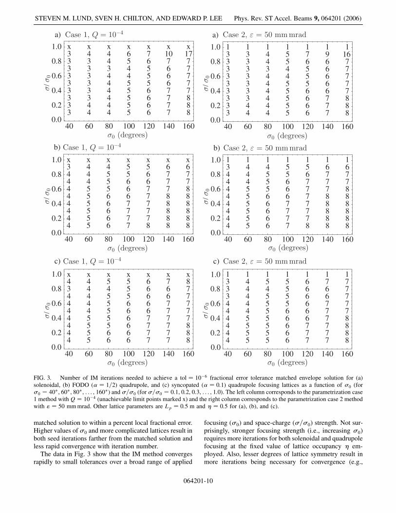
FIG. 3. Number of IM iterations needed to achieve a tol � 10�6 fractional error tolerance matched envelope solution for (a)solenoidal, (b) FODO (� � 1=2) quadrupole, and (c) syncopated (� � 0:1) quadrupole focusing lattices as a function of �0 (for�0 � 40, 60, 80, . . . , 160) and �=�0 (for �=�0 � 0:1, 0:2, 0:3, . . . , 1:0). The left column corresponds to the parametrization case1 method with Q � 10�4 (unachievable limit points marked x) and the right column corresponds to the parametrization case 2 methodwith " � 50 mm mrad. Other lattice parameters are Lp � 0:5 m and � 0:5 for (a), (b), and (c).

STEVEN M. LUND, SVEN H. CHILTON, AND EDWARD P. LEE Phys. Rev. ST Accel. Beams 9, 064201 (2006)

matched solution to within a percent local fractional error.Higher values of�0 and more complicated lattices result inboth seed iterations farther from the matched solution andless rapid convergence with iteration number.

The data in Fig. 3 show that the IM method convergesrapidly to small tolerances over a broad range of applied

064201

focusing (�0) and space-charge (�=�0) strength. Not sur-prisingly, stronger focusing strength (i.e., increasing �0)requires more iterations for both solenoidal and quadrupolefocusing at the fixed value of lattice occupancy em-ployed. Also, lesser degrees of lattice symmetry result inmore iterations being necessary for convergence (e.g.,

-10

0.0 0.2 0.4 0.6 0.8 1.0

7.2

7.4

7.6

7.8

8.0

8.2

s/L p

r0x

r1x

rx

κxr x(m

m)

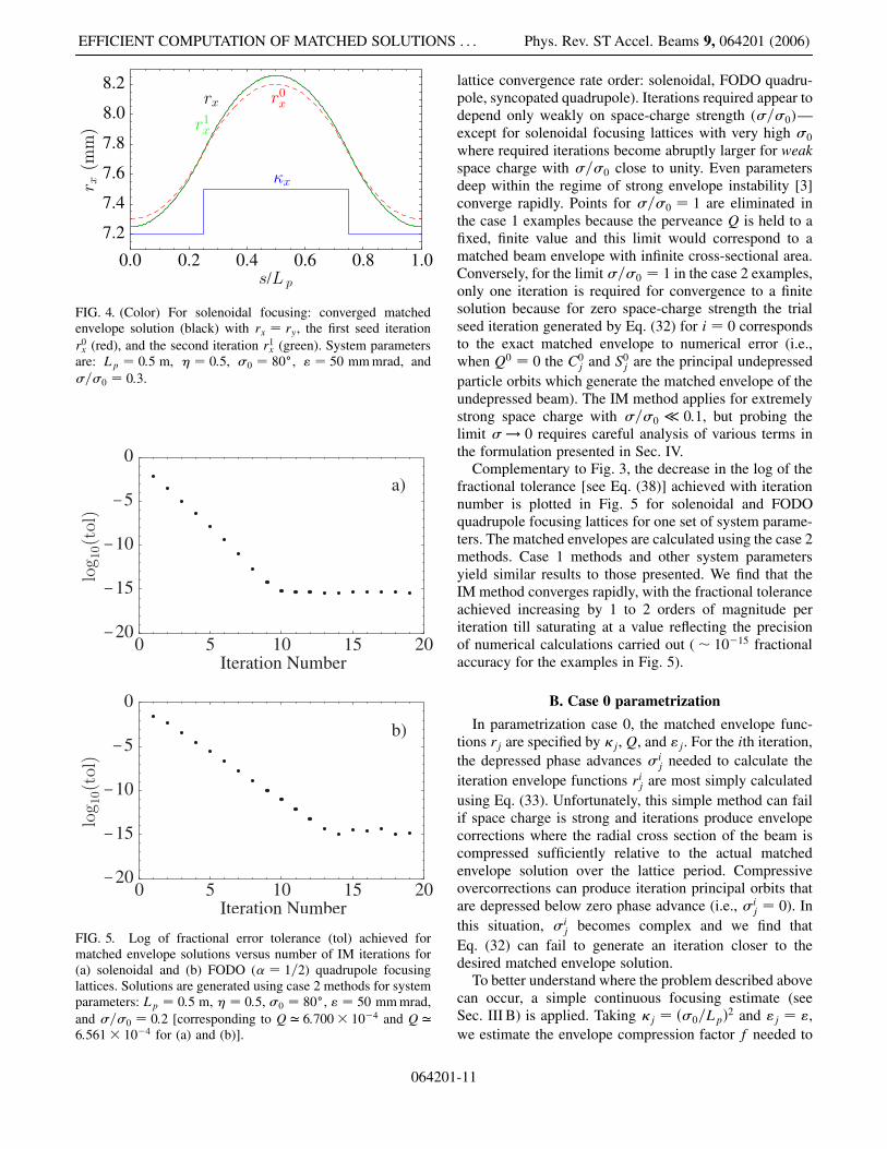
FIG. 4. (Color) For solenoidal focusing: converged matchedenvelope solution (black) with rx � ry, the first seed iterationr0x (red), and the second iteration r1

x (green). System parametersare: Lp � 0:5 m, � 0:5, �0 � 80, " � 50 mm mrad, and�=�0 � 0:3.

0

0

5

5

10

10

15

15

20

20

Iteration Number

Iteration Number

b)

a)

−

−

20

20

−

−

15

15

−

−

10

10

−

−

5

5

0

0

log

10(t

ol)

log

10(t

ol)

FIG. 5. Log of fractional error tolerance (tol) achieved formatched envelope solutions versus number of IM iterations for(a) solenoidal and (b) FODO (� � 1=2) quadrupole focusinglattices. Solutions are generated using case 2 methods for systemparameters: Lp � 0:5 m, � 0:5, �0 � 80, " � 50 mm mrad,and �=�0 � 0:2 [corresponding to Q ’ 6:700 10�4 and Q ’6:561 10�4 for (a) and (b)].

EFFICIENT COMPUTATION OF MATCHED SOLUTIONS . . . Phys. Rev. ST Accel. Beams 9, 064201 (2006)

064201

lattice convergence rate order: solenoidal, FODO quadru-pole, syncopated quadrupole). Iterations required appear todepend only weakly on space-charge strength (�=�0)—except for solenoidal focusing lattices with very high �0

where required iterations become abruptly larger for weakspace charge with �=�0 close to unity. Even parametersdeep within the regime of strong envelope instability [3]converge rapidly. Points for �=�0 � 1 are eliminated inthe case 1 examples because the perveance Q is held to afixed, finite value and this limit would correspond to amatched beam envelope with infinite cross-sectional area.Conversely, for the limit �=�0 � 1 in the case 2 examples,only one iteration is required for convergence to a finitesolution because for zero space-charge strength the trialseed iteration generated by Eq. (32) for i � 0 correspondsto the exact matched envelope to numerical error (i.e.,when Q0 � 0 the C0

j and S0j are the principal undepressed

particle orbits which generate the matched envelope of theundepressed beam). The IM method applies for extremelystrong space charge with �=�0 � 0:1, but probing thelimit �! 0 requires careful analysis of various terms inthe formulation presented in Sec. IV.

Complementary to Fig. 3, the decrease in the log of thefractional tolerance [see Eq. (38)] achieved with iterationnumber is plotted in Fig. 5 for solenoidal and FODOquadrupole focusing lattices for one set of system parame-ters. The matched envelopes are calculated using the case 2methods. Case 1 methods and other system parametersyield similar results to those presented. We find that theIM method converges rapidly, with the fractional toleranceachieved increasing by 1 to 2 orders of magnitude periteration till saturating at a value reflecting the precisionof numerical calculations carried out (� 10�15 fractionalaccuracy for the examples in Fig. 5).

B. Case 0 parametrization

In parametrization case 0, the matched envelope func-tions rj are specified by �j, Q, and "j. For the ith iteration,the depressed phase advances �ij needed to calculate theiteration envelope functions rij are most simply calculatedusing Eq. (33). Unfortunately, this simple method can failif space charge is strong and iterations produce envelopecorrections where the radial cross section of the beam iscompressed sufficiently relative to the actual matchedenvelope solution over the lattice period. Compressiveovercorrections can produce iteration principal orbits thatare depressed below zero phase advance (i.e., �ij � 0). Inthis situation, �ij becomes complex and we find thatEq. (32) can fail to generate an iteration closer to thedesired matched envelope solution.

To better understand where the problem described abovecan occur, a simple continuous focusing estimate (seeSec. III B) is applied. Taking �j � ��0=Lp�2 and "j � ",we estimate the envelope compression factor f needed to

-11

40

40

60

60

80

80

100

100

120

120

140

140

160

160

0.0

0.0

b)

a)

0.2

0.2

0.4

0.4

0.6

0.6

0.8

0.8

1.0

1.0

1

1

3

5

5

9

10

17

53

90

x

x

x

x

x

x

x

x

x

x

1

1

4

6

6

9

12

18

67

89

x

x

x

x

x

x

x

x

x

x

1

1

4

6

7

9

14

18

77

76

x

x

x

x

x

x

x

x

x

x

1

1

5

6

8

9

15

17

82

57

x

x

x

x

x

x

x

x

x

x

1

1

5

5

9

8

16

14

81

38

x

x x

x

x

x

x

x

x

x

x

1

1

6

6

9

7

16

11

68

22

x

x

x

x

x

x

x

x

1

x

10

1

8

9

9

10

15

15

63

44

x

x

x

x

x

x

x

xx

σ0 (degrees)

σ0 (degrees)

σ/σ

0σ

/σ0

FIG. 6. Number of conventional IM iterations needed in case 0to achieve a tol � 10�6 fractional error tolerance matchedenvelope solution for (a) solenoidal and (b) FODO (� � 1=2)quadrupole lattices as a function of �0 (for �0 � 40, 60, 80,. . . , 160) and �=�0 (for �=�0 � 0:1, 0:2, 0:3, . . . , 1:0). Systemparameters are: Lp � 0:5 m, � 0:5, and " � 50 mm mrad.Parameters where the method fails are marked x.

STEVEN M. LUND, SVEN H. CHILTON, AND EDWARD P. LEE Phys. Rev. ST Accel. Beams 9, 064201 (2006)

fully depress particle orbits within the matched envelope.A particle moving within the continuous matched enveloperj � rb has depressed phase advance ��=Lp�2 ���0=Lp�

2 �Q=rb2. Replacing rb ! frb and �! 0 in

this phase advance formula gives

f �

���2p

������������������������������������������������������1�

�����������������������������������������1� 4��0"=�QLp��

2qr : (41)

But for continuous focusing, we have [3]

�0"QLp

���=�0�

1� ��=�0�2 : (42)

Together, Eqs. (41) and (42) show that f � 0:99, 0:95, and0:90 (corresponding to �1%, 5%, and 10% compressiveovercorrections) will produce fully depressed particle or-bits for �=�0 < 0:14, 0:31, and 0:44. Numerically ana-lyzed examples below indicate that this problem can occurin periodic focusing lattices for more moderate spacecharge and compression factors than these continuousfocusing estimates suggest.

The parameter region where the IM method can beapplied using the ‘‘conventional’’ case 0 procedure forexample periodic solenoid and FODO quadrupole latticesis illustrated in Fig. 6. The region of applicability corre-sponds to parameters where Eq. (33) can be employed tocalculate the iteration depressed phases advances �ij with-out obtaining complex values. Iterations necessary toachieve tolerance are plotted as a function of �0 and�=�0. Rather than plotting results in terms of the per-veance Q, Eq. (14) was used to calculate �=�0 from thematched envelope functions and system parameters tobetter quantify the relative space-charge strength wherethe method fails. Values of Q were chosen to uniformlydistribute points in �=�0. Note that the IM method workswith the simple initial seed iteration when space charge ismoderate to weak (0:6<�=�0 � 1) but abruptly failswith increasing space charge (�=�0 < 0:6). Near the pointof failure, convergence becomes slow (iteration counts forthe examples in Fig. 6 can become thousands if points arechosen sufficiently close to the failure region).

Several alternative methods were attempted to render theIM method applicable to all case 0 parameters with arbi-trary space-charge strength. We formulate these methodswithout reference to a specific lattice or taking �0x � �0y

and "x � "y to better reflect general case 0 applications.First, rather than employing Eq. (33) to calculate the de-pressed phase advance �ij of the iteration, the integralformula (14) is applied with the envelope functions ofthe previous i� 1 iteration with

�ij � "jZ si�Lp

si

ds

�ri�1j �s��

2 : (43)

The anticipation is that �ij calculated from Eq. (43) should

064201

be sufficiently close to the actual depressed phase advance�j of the converged solution to correct the problem.Unfortunately, this method, when applied to the examplesolenoid and quadrupole lattices, results in systematicconvergence to unphysical solutions. Replacing Eq. (43)with an ‘‘under-relaxed’’ average over previous iterationsmight address this problem. In cases where complex phaseadvances resulted, various other simple replacements ofEq. (33) have been attempted without obtaining satisfac-tory results.

Several alternative procedures extend applicability togeneral case 0 parameters. First, slowly increasing theperveance Q from some sufficiently small (or zero) valuewhile implementing the conventional case 0 iterationmethod using Eq. (33) proves workable in our tests. Inthis scheme, if Eq. (33) fails (i.e., produces unphysicalcomplex values for �ij), then Q is adaptively decreasedwhile iterating until the formula becomes valid before

-12

40

40

60

60

80

80

100

100

120

120

140

140

160

160

0.0

0.0

0.2

0.2

0.4

0.4

0.6

0.6

0.8

0.8

1.0b)

1.0a)

1

1

9

9

10

9

10

9

10

9

10

9

10

9

10

9

10

7

10

7

1

1

16

21

23

9

15

9

15

9

17

9

15

9

13

9

11

10

11

10

1

1

16

14

17

10

15

9

15

10

16

10

16

10

14

10

16

10

12

10

1

1

19

14

18

15

18

12

18

14

16

15

16

11

17

11

17

11

17

11

1

1

18

24

19

16

20

32

21

15

19

15

19

16

19

16

17

16

16

12

1

1

22

30

20

37

21

18

23

16

38

16

22

20

20

19

20

17

18

13

1

1

22

56

23

23

23

21

23

19

24

21

22

19

22

32

22

20

18

18

σ0 (degrees)

σ0 (degrees)

σ/σ

0σ

/σ0

FIG. 7. Number of total hybrid IM iterations needed for case 0using tol � 10�6 fractional error tolerance case 1 matchedenvelope solutions and root found "j with 10�4 fractionalaccuracy from specified values for (a) solenoidal and (b)FODO (� � 1=2) quadrupole lattices. The same system parame-ters and presentation format are employed as in Fig. 6.

EFFICIENT COMPUTATION OF MATCHED SOLUTIONS . . . Phys. Rev. ST Accel. Beams 9, 064201 (2006)

increasing Q again toward the target value. For strongspace charge this procedure can result in many iterationsbeing necessary for convergence because small increasesinQwere required in various test cases examined. It is alsodifficult to determine optimal increments to increase theperveance—which complicates practical code develop-ment and can limit the range of method applicability.

Another, simpler to implement, alternative procedure isformulated by combining the Sec. VA method for solvingcase 1 parametrizations with numerical root finding. In this‘‘hybrid’’ procedure, the emittances "j calculated from thex- and y-plane constraint equations (23) are regarded as anundetermined function of the �j [i.e., "jjspecified �

"j��x; �y�] and trial matched envelope solutions rj arerapidly calculated to tolerance using matched envelopesobtained with case 1 methods for specified (guessed) val-ues of the �j. Numerical root finding can be employed torefine the guessed values for the �j to obtain the values of�j consistent with the target values of "j. Because the"j��x; �y� are smooth, monotonic functions of the �j for0<�j < �0j, the consistent values of the �j can be foundwith relatively small numbers of root finding iterations.This is particularly true for plane-symmetric systems(�0j � �0 and "j � ") because one-dimensional root find-ing can be employed.

The total number of two-dimensional (i.e., the calcula-tions do not assume plane symmetry) iterations needed toimplement this hybrid method for case 0 is shown in Fig. 7for example periodic solenoid and FODO quadrupole lat-tices. Here, the total iteration number represents the sum ofall iterations needed to calculate the emittances to a speci-fied fractional tolerance while calculating all trial matchedenvelope solutions to a separate specified tolerance over alltwo-dimensional root finding steps. The same lattices andpresentation methods used in Fig. 6 are employed to aidcomparisons. Note that the full case 0 parameter space isaccessible in this procedure with only relatively modesttotal iteration counts in spite of the additional numericalwork resulting from the root finding. A secantlike multi-dimensional root finding method is employed [16]. Notethat only two-dimensional root finding is necessary incontrast to four-dimensional root finding associated withconventional procedures for constructing matched enve-lope solutions by finding appropriate initial envelope co-ordinates and angles. Initial root finding iterations areseeded using continuous focusing model estimates for �jcalculated from Eq. (28) using the seed values of rj.Subsequent root finding steps in �j employ the previousstep matched envelopes as a seed envelope in the case 1iterations. For small root finding steps in �j this previousstep seeding saves considerable numerical work. Only oneiteration is necessary for the limit points with �=�0 � 1because for zero space-charge strength the trial seed itera-tion is exact to numerical error. Iteration counts at fixed �0

064201

likely increase and decrease in �=�0 due to approximateiteration seed guesses being (accidentally) farther andnearer to the actual root than in other cases. If the planesymmetries are employed (i.e., using "x � "y and �x ��y), then total iterations required can be further reduced.Matched envelopes for general case 0 parameters can alsobe calculated in similar values of total iterations by anal-ogously combining case 2 methods with numerical rootfinding. In this case 2 hybrid method, values of �j con-sistent with specified values of Q are calculated using thetwo components of Eq. (23) [i.e., set Q! Qj in the j � xand y components of Eq. (23) and then root solve for �jconsistent with Q � Qj��x; �y�].

VI. CONCLUSIONS

An iterative matching (IM) method for numerical cal-culation of the matched beam envelope solutions to the KV

-13

STEVEN M. LUND, SVEN H. CHILTON, AND EDWARD P. LEE Phys. Rev. ST Accel. Beams 9, 064201 (2006)

equations has been developed. The method is based onorbit consistency conditions between depressed particleorbits within a KV beam distribution and the envelope oforbits making up the distribution. Application of the IMmethod in simplest form requires numerical solution oflinear ordinary differential equations describing principalparticle orbits over one lattice period and the calculation ofa few axillary integrals over the lattice period. A largebasin of convergence enables seeding of the iterationswith a simple trial solution that takes into account boththe envelope flutter driven by the applied focusing latticeand leading-order space-charge defocusing forces. Allcases of envelope parametrizations can be employed, butthe method is most naturally expressed, and highly con-vergent, when employing the depressed particle phaseadvances �j as parameters—which also corresponds to anatural choice of parameters to employ for enhanced phys-ics understanding. Virtues of the IM method are: it isstraightforward to code and applicable to periodic focusinglattices of arbitrary complexity; it is efficient for arbitraryspace-charge intensity; and it works for all physicallyachievable system parameters—even in bands of paramet-ric envelope instability where conventional matching pro-cedures can fail.

ACKNOWLEDGMENTS

The authors wish to thank J. J. Barnard and A. Friedmanfor useful discussions. This research was performed underthe auspices of the U.S. Department of Energy at theLawrence Livermore and Lawrence Berkeley NationalLaboratories under Contracts No. W-7405-Eng-48 andNo. DE-AC03-76SF0098.

APPENDIX: MATCHED ENVELOPESYMMETRIES FOR QUADRUPOLE DOUBLET

AND SOLENOIDAL FOCUSING

Consider a periodic quadrupole doublet lattice [3] focus-ing a beam with equal x- and y-plane emittances (i.e., "x �"y). To concretely define doublet focusing, we assume thatan s-coordinate origin can be chosen such that the latticefocusing functions �j�s� satisfy

�j�s� � ��j��s�; (A1)

in addition to the general quadrupole lattice symmetry�x � ��y. This doublet focusing symmetry is consistentwith focusing/defocusing elements with axial structure(i.e., including fringe fields) if both the focusing anddefocusing elements are realized by identical hardwareassemblies with equal field excitations appropriately ar-ranged in a regular lattice via symmetry operations (i.e.,translations and rotations). Note that s � 0 corresponds tothe axial location of the drift between two successivequadrupoles in the periodic lattice (for cases where a finitefringe field extends into the drifts, this location will be

064201

where �j � 0). Assume that the matched envelope func-tions satisfying the KV equation (1) are symmetric aboutthe mid-drift with

rj�s� � r~j��s�: (A2)

Here, if j � x; y, then ~j � y; x. Take the j � x KV equa-tion [see Eq. (1)], substitute s! �s. Then employing thefocusing and envelope symmetries in Eqs. (A1) and (A2)together with �y � ��x obtains the complementary j � yKV equation, thereby showing that the assumed symmetryin Eq. (A2) is consistent. An immediate corollary ofEq. (A2) is that at any mid-drift between quadrupoles,the envelope is round (i.e., rx � ry) with opposite conver-gence angles (i.e., r0x � �r0y).

Restrict the situation described above to a symmetricFODO system where the focusing and defocusing quadru-poles of the doublet are separated by equal length axialdrifts [3] and the focusing and defocusing elements areeach reflection symmetric about their axial midpoint [i.e.,within one element, �x�s� ~s� � �x��s� ~s� where s � ~sis the geometric field center of the element]. These furtherassumptions lead to the additional FODO focusing sym-metry

�j�s� � �~j�Lp=2� s�: (A3)

With the choice of s � 0 made as above, the focusing anddefocusing optical elements are centered at s � Lp=4 ands � 3Lp=4 within the period s 2 �0; Lp�. Using stepsanalogous to those outlined above, it can be shown thatthe matched envelope functions also have the FODO sym-metry:

rj�s� � r~j�Lp=2� s�: (A4)

Another FODO symmetry can be obtained by replacings! �s in Eq. (A4), applying Eq. (A2), and differentiatingto yield

r0j�s� � �r0j�Lp=2� s�: (A5)

Evaluating this expression at the focusing element centersat s � Lp=4 and s � 3Lp=4 and invoking periodicity ofthe rj with r0j�s� Lp� � r0j�s� shows that the matchedenvelope functions are extremized (i.e., r0j � 0) at thefocusing element centers in a symmetric FODO lattice.The envelope equation (1) then shows that the j-planeextrema of rj with �j < 0 (defocusing plane) satisfies r00j >0 and therefore must be a minimum value. Period symme-tries then require that the other focusing plane extrema(~j-plane with �~j > 0) corresponds to a maximum value.

Analogous steps to those employed in the analysis ofquadrupole doublet focusing can be applied to solenoidalfocusing (�x � �y) systems with "x � "y to show that

-14

EFFICIENT COMPUTATION OF MATCHED SOLUTIONS . . . Phys. Rev. ST Accel. Beams 9, 064201 (2006)

rx � ry. Consider a periodic solenoidal focusing functionwith only a single element in the period that is also reflec-tion symmetric about the axial midplane (with reflectionsymmetry defined as for the FODO quadrupole caseabove). Then procedures used above are readily employedto show that the matched envelope function rj is maximumat the axial center of the focusing element and is minimumat the axial center of the drift.

[1] I. Kapchinskij and V. Vladimirskij, in Proceedings of theInternational Conference on High Energy Acceleratorsand Instrumentation (CERN Scientific InformationService, Geneva, 1959), p. 274.

[2] M. Reiser, Theory and Design of Charged Particle Beams(John Wiley & Sons, Inc., New York, 1994).

[3] S. M. Lund and B. Bukh, Phys. Rev. ST Accel. Beams 7,024801 (2004).

[4] R. Ryne, Technical Report acc-phys/9502001, http://arxiv.org, Accelerator Physics (1995).

[5] H. Wiedemann, Particle Accelerator Physics: BasicPrinciples and Linear Beam Dynamics (Springer-Verlag,New York, 1993).

[6] E. P. Lee, Part. Accel. 52, 115 (1996).[7] E. P. Lee, Phys. Plasmas 9, 4301 (2002).

064201

[8] O. Anderson, in Proceedings of the 2005 ParticleAccelerator Conference, Knoxville, TN (IEEE,Piscataway, NJ, 2005), p. TPAT061.

[9] O. A. Anderson (to be published).[10] R. C. Davidson, Physics of Nonneutral Plasmas (Addison-

Wesley, Reading, MA, 1990), rereleased, World Scientific,2001.

[11] I. Hofmann, L. J. Laslett, L. Smith, and I. Haber, Part.Accel. 13, 145 (1983).

[12] E. D. Courant and H. S. Snyder, Ann. Phys. (Leipzig) 3, 1(1958).

[13] E. Lee and R. J. Briggs, Technical Report LBNL-40774,UC-419, Lawrence Berkeley National Laboratory,1997.

[14] R. C. Davidson and Q. Qian, Phys. Plasmas 1, 3104(1994).

[15] R. C. Davidson and H. Qin, Physics of Intense ChargedParticle Beams in High Energy Accelerators (WorldScientific, New York, 2001).

[16] S. Wolfram, The Mathematica Book (Wolfram Media,Champaign, IL, 2003), 5th ed.

[17] S. M. Lund, S. H. Chilton, and E. P. Lee, http://arxiv.org/abs/physics/0602150.

[18] See EPAPS Document No. E-PRABFM-9-005606 forprograms and supplementary material. For more informa-tion on EPAPS, see http://www.aip.org/pubservs/epaps.html.

-15