Efﬁcient Algorithms for Maximum Regression … Comput Geom ... Efﬁcient Algorithms for Maximum...

Discrete Comput Geom (2008) 39: 656–677DOI 10.1007/s00454-007-9046-6

Efficient Algorithms for Maximum Regression Depth

Marc van Kreveld · Joseph S.B. Mitchell ·Peter Rousseeuw · Micha Sharir · Jack Snoeyink ·Bettina Speckmann

Received: 5 September 2005 / Revised: 3 December 2007 /Accepted: 3 December 2007 / Published online: 21 December 2007© The Author(s) 2007

A preliminary version of this paper appeared in the proceedings of the 15th Annual ACMSymposium on Computational Geometry (1999)

M. van Kreveld partially funded by the Netherlands Organization for Scientific Research (NWO)under FOCUS/BRICKS grant number 642.065.503.J.S.B. Mitchell’s research largely conducted while the author was a Fulbright Research Scholarat Tel Aviv University. The author is partially supported by NSF (CCR-9504192,CCR-9732220), Boeing, Bridgeport Machines, Sandia, Seagull Technology, and SunMicrosystems.M. Sharir supported by NSF Grants CCR-97-32101 and CCR-94-24398, by grants from theU.S.–Israeli Binational Science Foundation, the G.I.F., the German–Israeli Foundation forScientific Research and Development, and the ESPRIT IV LTR project No. 21957 (CGAL), andby the Hermann Minkowski—MINERVA Center for Geometry at Tel Aviv University.J. Snoeyink supported in part by grants from NSERC, the Killam Foundation, and CIES while atthe University of British Columbia.

M. van Kreveld (�)Department of Information and Computing Sciences, Utrecht University, Utrecht, TheNetherlandse-mail: [email protected]

J.S.B. MitchellDepartment of Applied Mathematics and Statistics, SUNY Stony Brook, Stony Brook, USAe-mail: [email protected]

P. RousseeuwDepartment of Mathematics and Computer Science, Universitaire Instelling Antwerpen,Antwerpen, Belgiume-mail: [email protected]

M. SharirSchool of Computer Science, Tel Aviv University, Tel Aviv, Israele-mail: [email protected]

J. SnoeyinkDepartment of Computer Science, UNC Chapel Hill, Chapel Hill, USAe-mail: [email protected]

B. SpeckmannDepartment of Mathematics and Computer Science, TU Eindhoven, Eindhoven, The Netherlandse-mail: [email protected]

mailto:[email protected]






Discrete Comput Geom (2008) 39: 656–677 657

Abstract We investigate algorithmic questions that arise in the statistical problemof computing lines or hyperplanes of maximum regression depth among a set of n

points. We work primarily with a dual representation and find points of maximumundirected depth in an arrangement of lines or hyperplanes. An O(nd) time andO(nd−1) space algorithm computes undirected depth of all points in d dimensions.Properties of undirected depth lead to an O(n log2 n) time and O(n) space algorithmfor computing a point of maximum depth in two dimensions, which has been im-proved to an O(n logn) time algorithm by Langerman and Steiger (Discrete Comput.Geom. 30(2):299–309, 2003). Furthermore, we describe the structure of depth in theplane and higher dimensions, leading to various other geometric and algorithmic re-sults.

1 Introduction

The notion of the depth of a point with respect to a set of point data is importantin statistical analysis. Several proposals for depth have been made which include,for example, Tukey depth, Oja depth, simplicial and convex-layers depth, as wellas regression depth. Because of its application to statistics the design of algorithmsfor the computation of points of maximal or minimal depths (depending on the pre-cise definition) has attracted a great deal of attention in the Computational Geometrycommunity in recent years. See [7, 29] and the references therein for the precise def-initions of these depth measures and an overview of the contribution of ComputationGeometry to the computation of robust statistics.

Motivated by the study of robust regression in statistics [18, 24–28, 30, 32, 33],Peter Rousseeuw posed the question of computing maximum regression depth in hisinvited talk at the 14th ACM Symposium on Computational Geometry: Given a set P

of n points in the plane, the regression depth of a line is the minimum number ofpoints that must be removed from P to allow the line to rotate about a pivot point onthe line to a vertical position without ever containing a remaining point of P .7 Thisdefinition is given more generally in the next section.

A line (or hyperplane) of maximum depth has statistical properties that are desir-able as a robust regression estimator [1, 2]. The experimental investigation of theseproperties has been hampered by the inefficiency of the straightforward algorithmsfor computing maximum depth. These required Θ(n3) time in the plane [26] andΘ(n2d−1 logn) time in dimensions d ≥ 3 [25, 28].

In the next section, we define an equivalent dual problem, computing undirecteddepth in an arrangement of lines or hyperplanes. The properties of undirected depthwill lead to an O(nd) algorithm for computing regression depth for all dimensions.In Sect. 3, we focus on arrangements in the plane and we present an algorithm tocompute a cell of maximum depth in O(n log2 n) time. Langerman and Steiger sub-sequently improved this to O(n logn) time, but as their algorithm is based on ourapproach and lemmas, we think it is important to present our algorithm neverthe-less. In Sect. 4, we continue the analysis of depth with algorithms to determine the

7Rousseeuw also posed a combinatorial question, resolved by Amenta et al. [3], who show that for any set

of n points in Rd , there exists a hyperplane with regression depth at least �n/(d + 1)�.

658 Discrete Comput Geom (2008) 39: 656–677

deepest vertex in an arrangement, show a connection with k-sets, and deal with depthin degenerate arrangements. In Sect. 5, we comment on computing depth in higherdimensions, and show how to reduce space requirements from O(nd) to O(nd−1).

2 Duality and Undirected Depth in Arrangements

Although regression depth is defined for a line or hyperplane among n points, itis easier to work with a duality transformation that maps points to hyperplanesand vice versa. We use the duality from Edelsbrunner’s book [13]: an inversionabout the unit paraboloid xd = x2

1 + x22 + · · · + x2

d−1 that maps a point p =(p1,p2, . . . , pd) to the hyperplane pD : xd = 2p1x1 +2p2x2 +· · ·+2pd−1xd−1 −pd

and maps a hyperplane h : xd = a1x1 + a2x2 + · · · + ad−1xd−1 + b to the pointhD = (a1/2, a2/2, . . . , ad−1/2,−b). This duality preserves point/line incidence andabove/below relationships. Note that the duality mapping will neither accept nor pro-duce vertical hyperplanes, which have equations that do not involve the variable xd .

All rotations of a hyperplane h can be generated as follows. Choose a set Q of d

affinely independent points whose affine hull is h. Move one of the points q0 ∈ Q byincreasing (or decreasing) its last coordinate toward infinity. If the points Q are stilltaken to span h, then h rotates toward the vertical about the (d − 1)-flat spanned bypoints of Q \ {q0}.

The dual of a rotation is easy to interpret. The points of Q map to hyperplanesthrough a common point hD . Hyperplane q0

D moves parallel to itself up (or down)the xd axis, so the point common to all hyperplanes moves from hD toward infinityalong a ray that is contained in the duals of the stationary points.

Given n primal points P , the number that must be removed to allow a particularrotation are the number that are passed over by the rotation, plus the number that areon the final vertical plane (which our rotation never reaches). This number can becounted in the dual as the number of hyperplanes dual to points in P that are crossedby the ray corresponding to the rotation, plus the number of hyperplanes parallel tothe ray. Therefore, for an arrangement of n hyperplanes A, we define the undirecteddepth, or just depth, of a point p to be the minimum number of hyperplanes inter-sected by some ray from p, counting parallel hyperplanes as intersecting at infinity.Hyperplanes containing p are counted for all rays. For the rest of this paper we focuson computing depth of a point in an arrangement of n lines or hyperplanes.

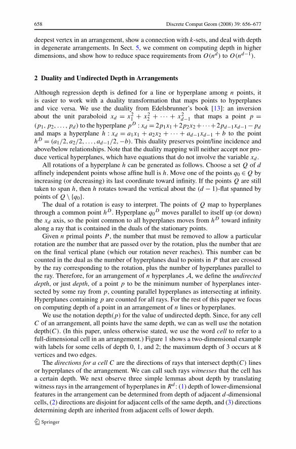
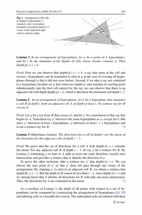
We use the notation depth(p) for the value of undirected depth. Since, for any cellC of an arrangement, all points have the same depth, we can as well use the notationdepth(C). (In this paper, unless otherwise stated, we use the word cell to refer to afull-dimensional cell in an arrangement.) Figure 1 shows a two-dimensional examplewith labels for some cells of depth 0, 1, and 2; the maximum depth of 3 occurs at 8vertices and two edges.

The directions for a cell C are the directions of rays that intersect depth(C) linesor hyperplanes of the arrangement. We can call such rays witnesses that the cell hasa certain depth. We next observe three simple lemmas about depth by translatingwitness rays in the arrangement of hyperplanes in Rd : (1) depth of lower-dimensionalfeatures in the arrangement can be determined from depth of adjacent d-dimensionalcells, (2) directions are disjoint for adjacent cells of the same depth, and (3) directionsdetermining depth are inherited from adjacent cells of lower depth.


Fig. 1 Arrangement with cellsof depth 0 (unbounded), 1(shaded), and 2 (unshaded,bounded); maximum depth of 3occurs at the indicated eightvertices and two edges

Lemma 1 In an arrangement of hyperplanes, let p be a point on k hyperplanes,and let i be the minimum of the depths of cells whose closure contains p. Thendepth(p) = i + k.

Proof First we can observe that depth(p) ≤ i + k: a ray that starts in the cell andcrosses i hyperplanes can be translated to start at p at the cost of crossing all hyper-planes through p that it did not cross before. Second, if we take a ray not containedin a hyperplane incident on p that witnesses depth(p) and translate its starting pointinfinitesimally into the first cell entered by the ray, we can observe that there is anadjacent cell with depth depth(p)−k, which is therefore the minimum cell depth i. �

Lemma 2 In an arrangement of hyperplanes, let h be a hyperplane that separatesa cell B of depth i from an adjacent cell A of depth at least i. No witness ray for B

crosses h.

Proof Let ρ be a ray from B that crosses h, and let ρ′ be a translation of this ray thatbegins in A. Translated ray ρ′ intersects the same hyperplanes as ρ, except for h. Butsince ρ′ intersects at least i hyperplanes, ρ intersects at least i + 1 hyperplanes andis not a witness ray for B . �

Lemma 3 (Inheritance lemma) The directions for a cell of depth i are the union ofthe directions for the adjacent cells of depth i − 1.

Proof We prove that the set of directions for a cell A with depth(A) = i containsthe union. For any adjacent cell B of depth i − 1, let ray ρ be a witness for B . ByLemma 2, translating ρ to start in A adds at most one (and, therefore, exactly one)intersection, and provides a witness that A inherits the direction of ρ.

To prove the other inclusion, take a witness ray ρ′ that depth(A) = i. We canchoose the start point of ρ′ so that ρ′ does not pass through any vertex of thearrangement. By clipping ρ′ to start in an adjacent cell B , we obtain a witness thatdepth(B) ≤ i−1. But the depth of B cannot be less than i−1, since depth(A) = i andwe already know that A inherits all directions for B with only one more intersection.Thus, the directions for A are contained in the union. �

As a corollary of Lemma 3, the depth of all points with respect to a set of hy-perplanes can be computed by constructing the arrangement of hyperplanes [14, 15]and labeling cells in a breadth-first search. The unbounded cells are labeled with their


depth zero. Then, for i = 1, 2, . . . , all cells with label i − 1 cause their adjacent, unla-beled cells to be labeled i. Finally, lower-dimensional cells can be labeled accordingto Lemma 1.

Corollary 4 For n hyperplanes in Rd , the depths of all cells, and thus the maxi-mum depth too, can be computed in O(nd) time by building the arrangement andtraversing the graph of adjacent cells.

3 An Algorithm for Maximum Depth Cells in the Plane

Undirected depth in two dimensions satisfies some additional properties that allow anefficient algorithm to compute a two-dimensional cell of maximum depth. Langermanand Steiger [21] built upon the results presented in this section to give an optimalalgorithm that finds a maximum depth cell in O(n logn) time and linear space.

Suppose that we are given a set L of n lines in the plane. We first consider nonde-generate sets of lines (arrangements of lines) only, that is, no line is vertical, no twolines are parallel, and no three lines pass through a single point. We will relax thisassumption in Sect. 4.5. Our goal is to find, among all the points of the plane thatdo not lie on lines of L, a point p whose depth is maximum. Note that vertices andedges of the arrangement A(L) may attain greater depth than p—we return to thesein Sect. 4.1.

We will use a binary search on x-coordinates of vertices of the arrangement A(L),with a test for which side of a vertical line contains a maximum depth cell. Section 3.1establishes properties that allow a sidedness test; Sect. 3.2 describes a tournamentdata structure needed to implement the sidedness test.

3.1 A Sidedness Test

In the plane, we use two concepts to determine which side of a vertical test line canhave cells of maximum depth: a wedge lemma and the notion of top directions.

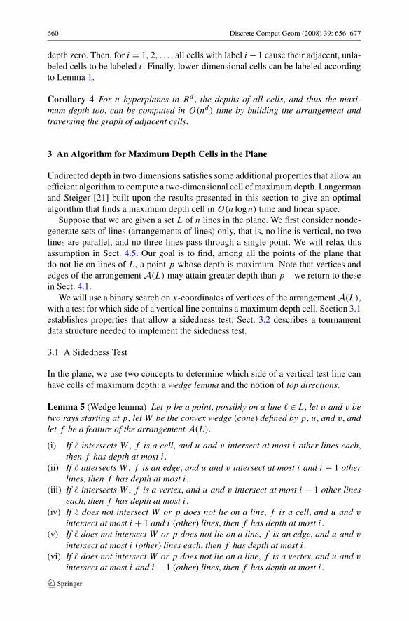
Lemma 5 (Wedge lemma) Let p be a point, possibly on a line � ∈ L, let u and v betwo rays starting at p, let W be the convex wedge (cone) defined by p, u, and v, andlet f be a feature of the arrangement A(L).

(i) If � intersects W , f is a cell, and u and v intersect at most i other lines each,then f has depth at most i.

(ii) If � intersects W , f is an edge, and u and v intersect at most i and i − 1 otherlines, then f has depth at most i.

(iii) If � intersects W , f is a vertex, and u and v intersect at most i − 1 other lineseach, then f has depth at most i.

(iv) If � does not intersect W or p does not lie on a line, f is a cell, and u and v

intersect at most i + 1 and i (other) lines, then f has depth at most i.(v) If � does not intersect W or p does not lie on a line, f is an edge, and u and v

intersect at most i (other) lines each, then f has depth at most i.(vi) If � does not intersect W or p does not lie on a line, f is a vertex, and u and v

intersect at most i and i − 1 (other) lines, then f has depth at most i.


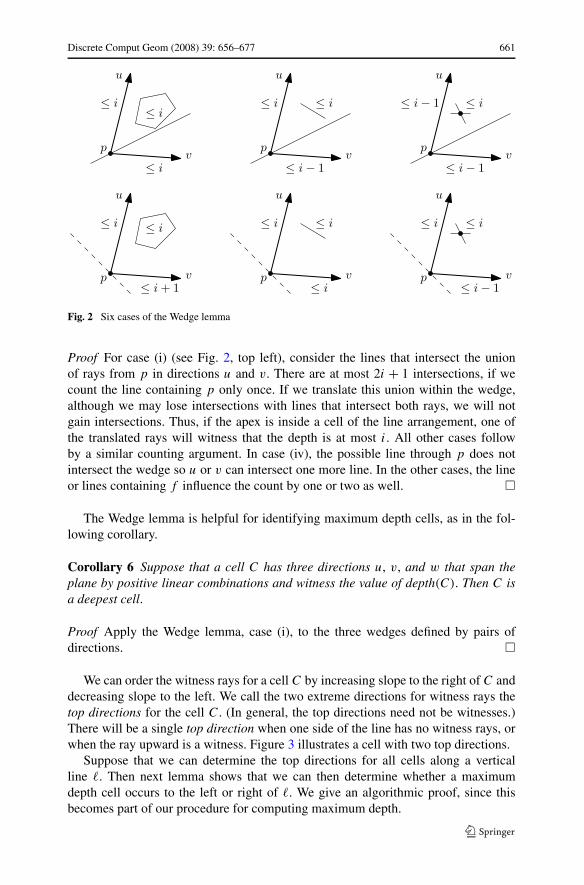
Fig. 2 Six cases of the Wedge lemma

Proof For case (i) (see Fig. 2, top left), consider the lines that intersect the unionof rays from p in directions u and v. There are at most 2i + 1 intersections, if wecount the line containing p only once. If we translate this union within the wedge,although we may lose intersections with lines that intersect both rays, we will notgain intersections. Thus, if the apex is inside a cell of the line arrangement, one ofthe translated rays will witness that the depth is at most i. All other cases followby a similar counting argument. In case (iv), the possible line through p does notintersect the wedge so u or v can intersect one more line. In the other cases, the lineor lines containing f influence the count by one or two as well. �

The Wedge lemma is helpful for identifying maximum depth cells, as in the fol-lowing corollary.

Corollary 6 Suppose that a cell C has three directions u, v, and w that span theplane by positive linear combinations and witness the value of depth(C). Then C isa deepest cell.

Proof Apply the Wedge lemma, case (i), to the three wedges defined by pairs ofdirections. �

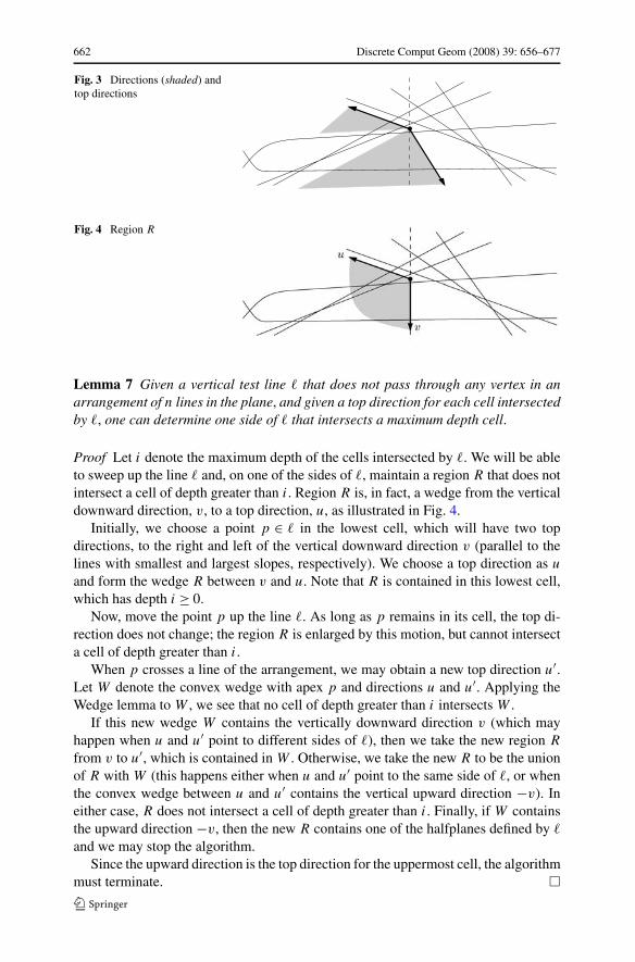
We can order the witness rays for a cell C by increasing slope to the right of C anddecreasing slope to the left. We call the two extreme directions for witness rays thetop directions for the cell C. (In general, the top directions need not be witnesses.)There will be a single top direction when one side of the line has no witness rays, orwhen the ray upward is a witness. Figure 3 illustrates a cell with two top directions.

Suppose that we can determine the top directions for all cells along a verticalline �. Then next lemma shows that we can then determine whether a maximumdepth cell occurs to the left or right of �. We give an algorithmic proof, since thisbecomes part of our procedure for computing maximum depth.


Fig. 3 Directions (shaded) andtop directions

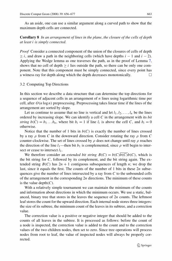
Fig. 4 Region R

Lemma 7 Given a vertical test line � that does not pass through any vertex in anarrangement of n lines in the plane, and given a top direction for each cell intersectedby �, one can determine one side of � that intersects a maximum depth cell.

Proof Let i denote the maximum depth of the cells intersected by �. We will be ableto sweep up the line � and, on one of the sides of �, maintain a region R that does notintersect a cell of depth greater than i. Region R is, in fact, a wedge from the verticaldownward direction, v, to a top direction, u, as illustrated in Fig. 4.

Initially, we choose a point p ∈ � in the lowest cell, which will have two topdirections, to the right and left of the vertical downward direction v (parallel to thelines with smallest and largest slopes, respectively). We choose a top direction as u

and form the wedge R between v and u. Note that R is contained in this lowest cell,which has depth i ≥ 0.

Now, move the point p up the line �. As long as p remains in its cell, the top di-rection does not change; the region R is enlarged by this motion, but cannot intersecta cell of depth greater than i.

When p crosses a line of the arrangement, we may obtain a new top direction u′.Let W denote the convex wedge with apex p and directions u and u′. Applying theWedge lemma to W , we see that no cell of depth greater than i intersects W .

If this new wedge W contains the vertically downward direction v (which mayhappen when u and u′ point to different sides of �), then we take the new region R

from v to u′, which is contained in W . Otherwise, we take the new R to be the unionof R with W (this happens either when u and u′ point to the same side of �, or whenthe convex wedge between u and u′ contains the vertical upward direction −v). Ineither case, R does not intersect a cell of depth greater than i. Finally, if W containsthe upward direction −v, then the new R contains one of the halfplanes defined by �

and we may stop the algorithm.Since the upward direction is the top direction for the uppermost cell, the algorithm

must terminate. �


As an aside, one can use a similar argument along a curved path to show that themaximum depth cells are connected.

Corollary 8 In an arrangement of lines in the plane, the closure of the cells of depthat least i is simply connected.

Proof Consider a connected component of the union of the closures of cells of depth≥ i, and draw a path in the neighboring cells (which have depths i − 1 and i − 2).Applying the Wedge lemma as one traverses the path, as in the proof of Lemma 7,shows that no cell of depth ≥ i lies outside the path, so there can be only one com-ponent. Note that this component must be simply connected, since every point hasa witness ray for depth along which the depth decreases monotonically. �

3.2 Computing Top Directions

In this section we describe a data structure that can determine the top directions fora sequence of adjacent cells in an arrangement of n lines using logarithmic time percell, after O(n logn) preprocessing. Preprocessing takes linear time if the lines of thearrangement are sorted by slope.

Let us continue to assume that no line is vertical and let l1, l2, . . . , ln be the linesordered by increasing slope. We can identify a cell C in the arrangement with its bitstring b(C) = b1 . . . bn, where bit bi = 1 if line li is above the cell C, and bi = 0otherwise.

Notice that the number of 1 bits in b(C) is exactly the number of lines crossedby a ray ρ from C in the downward direction. Consider rotating the ray ρ from C

counter-clockwise. The set of lines crossed by ρ does not change until ray ρ reachesthe direction of the line l1—then bit b1 is complemented, since ρ will begin to inter-sect or cease to intersect l1.

We therefore consider an extended bit string B(C) = b(C)b(C)b(C), which isthe bit string for C, followed by its complement, and the bit string again. The ex-tended string B(C) has 2n + 1 contiguous subsequences of length n; we drop thelast, since it equals the first. The counts of the number of 1 bits in these 2n subse-quences give the number of lines intersected by a ray from C to the unbounded cellsof the arrangement in the corresponding 2n directions. The minimum of these countsis the value depth(C).

With a relatively simple tournament we can maintain the minimum of the countsand information about directions in which the minimum occurs. We use a static, bal-anced, binary tree that stores in the leaves the sequence of 2n counts. The leftmostleaf stores the count for the upward direction. Each internal node stores three integers:the size of its subtree, the minimum count of the leaves in its subtree, and a correctionvalue.

The correction value is a positive or negative integer that should be added to thecounts of all leaves in the subtree. It is processed as follows: before the count ofa node is inspected, the correction value is added to the count and to the correctionvalues of the two children nodes, then set to zero. Since tree operations will processnodes from root to leaf, the value of inspected nodes will always be properly cor-rected.


The tree supports two operations: a query and an update. The query asks for theleaf with minimum count; in case of equal counts we want both the leftmost leafand the rightmost leaf with these counts—these give the top directions for the cell C.Since each internal node stores the minimum count in its subtree, such a query is easyto perform in O(logn) time by following two paths in the tree.

The update operation corresponds to moving from a cell C to a cell C′ by crossingsome line li . This means that the bit string of b(C′) differs from b(C) in the ith bit.In the extended string B(C′), three bits change to their complements. Since the 2n

counts for a cell are obtained by adding n consecutive bits, every count changes—ifbi changes from 0 to 1, then the first i counts increase by one, the next n countsdecrease by one, and the final n − i counts increase by one. Thus, we should notupdate the counts in the leaves explicitly, since this would take linear time; insteadwe update correction values.

We follow the two paths in the tree to the ith leaf and the (i + n)th leaf using thesize-of-subtree integers stored at the internal nodes. The paths partition the tree intothree parts. For all highest nodes left of the search path to the ith leaf we incrementthe correction value (or decrement, if bi changes from 1 to 0). This is done also forthe highest nodes right of the search path to the (i + n)th leaf. For the highest nodesbetween the search paths we decrement (or increment) the correction value. Sincethere can be at most O(logn) highest nodes left (or right) of any path in the tree, onlyO(logn) correction values are updated.

Because the structure of the tree is static, we implement it by indexing into a fixedarray, and subtree sizes are calculated rather than stored.

Lemma 9 Using the data structure described above, one can determine the top direc-tions for a sequence of adjacent cells in an arrangement of n lines using logarithmictime per cell, after O(n logn) preprocessing.

3.3 Binary Search for a Maximum Depth Cell

It is probably no surprise that we use the sidedness test in a binary search on x-coordinates of vertices of the arrangement A(L). A Java prototype can be seen atwww.win.tue.nl/~speckman/demos/maxdepth.

Standard results on slope selection [5, 10, 19, 22] allow us to consider the portionof the arrangement A(L) that lies between two vertical lines, and to generate thevertex of median x coordinate in O(n logn) time. We base our implementation ona randomized algorithm of Dillencourt, Mount, and Netanyahu [12].

At a vertical test line � through (or, rather, slightly near) this median vertex, we sortthe intersections with the lines of L and use the tournament described in Sect. 3.2 tocompute the depth of each point on the test line � and the top directions in O(n logn)

time. Lemma 7 then allows us to discard one side of the line �, and to continue thesearch on the other side. The search terminates when there are no intersection pointsremaining, which occurs after at most log(n2) = 2 logn steps. Thus, we claim thefollowing result.

Theorem 10 A cell of maximum undirected depth in an arrangement of n lines canbe computed in O(n log2 n) time and O(n) space.

http://www.win.tue.nl/~speckman/demos/maxdepth


As remarked before, Langerman and Steiger improved this result to O(n logn)

time [21]. They make use of the Wedge lemma presented here, but replace our sided-ness test by a version that is more efficient: in recursive steps, a constant fraction ofthe lines can be pruned out.

4 The Structure of Depth

Although our binary search identifies a deepest cell, we know from Lemma 1 thatthe maximum depth in an arrangement will always occur at a vertex. In statisticalanalysis, we may also wish to know the set of all lines with maximum regressiondepth, which corresponds to the set of all points at maximum depth. In this section,we characterize the set of points at maximum depth in nondegenerate arrangementsin the plane. We also establish relationships with k-sets in all dimensions and showhow to efficiently approximate a maximum depth point in degenerate arrangements.

4.1 Finding a Deepest Vertex in a Nondegenerate Arrangement

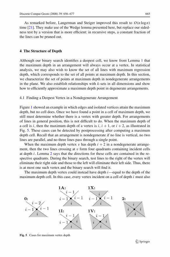
Figure 1 showed an example in which edges and isolated vertices attain the maximumdepth, but no cell does. Once we have found a point in a cell of maximum depth, westill must determine whether there is a vertex with greater depth. For arrangementsof lines in general position, this is not difficult to do. When the maximum depth ofa cell is i, then the maximum depth of a vertex is i, i + 1, or i + 2, as illustrated inFig. 5. These cases can be detected by postprocessing after computing a maximumdepth cell. Recall that an arrangement is nondegenerate if no line is vertical, no twolines are parallel, and no three lines pass through a single point.

When the maximum depth vertex v has depth i + 2 in a nondegenerate arrange-ment, then the two lines crossing at v form four quadrants containing incident cellsat depth i. Lemma 2 says that the directions for these cells are contained in the re-spective quadrants. During the binary search, test lines to the right of the vertex willeliminate their right side and those to the left will eliminate their left side. Thus, thereis at most one such vertex and the binary search will find it.

The maximum depth vertex could instead have depth i—equal to the depth of themaximum depth cell. In this case, every vertex incident on a cell of depth i must also

Fig. 5 Cases for maximum vertex depth


be incident on two cells of depth i − 1 and one of depth i − 2, otherwise the vertexdepth would be greater than i, as illustrated in Fig. 5. This, together with the fact thatcells are convex and the maximum depth is connected, implies that there can be onlyone cell that attains the maximum, which will be found by our binary search.

Finally if the maximum depth vertex has depth i + 1, then every cell of depth i

has to have at least one incident vertex of depth i + 1. This follows, e.g., from thecase analysis shown in Fig. 5, and from the fact that the set of points at depth ≥ i isconnected. Since our binary search finds a cell of depth i a traversal of its boundarywill yield a vertex of depth i + 1.

Theorem 11 After computing a deepest cell, one can compute a deepest vertex inO(n logn) additional time.

Proof Once we have computed some cell of maximum depth i, we must determinewhether a maximum depth vertex has depth i, i +1, or i +2. This is most easily doneby constructing the cell as the intersection of the n halfplanes that are defined by linesof the arrangement and that contain the cell. Intersection is equivalent to convex hullcomputation, and takes O(n logn) time. Then we can use the tournament to checkthe depth of all vertices, also in O(n logn) time. By the above discussion, we eitherfind that all vertices are of depth i, or there is a unique vertex of depth i + 2, or somevertex is of depth i + 1. �

4.2 Connections with k-Sets

It is natural to ask for the set of all points with maximum undirected depth, whichcorresponds to the set of all lines that have maximum regression depth. This appearsto be more difficult; in this section we observe the connections between the complex-ity of points with given undirected depth and the concept of k-sets in a configurationof points. There has been considerable attention in computational geometry devotedto k-sets, and the dual concept of k-levels in an arrangement of lines or hyperplanes;see, e.g., [9, 11, 13, 23, 31].

The k-level of an arrangement A for a particular direction θ consists of all pointsp such that a ray from p in direction θ intersects exactly k hyperplanes. (Usually,hyperplanes containing p are not counted.) In the dual, the k intersected hyperplanesbecome a k-set: k points that can be separated from the configuration by an open half-space bounded by a hyperplane, namely pD . Note that point p has undirected depthat most k (assuming that p does not lie on any hyperplane) and that the hyperplanepD has regression depth at most k as shown by rotation about any line outside theconvex hull of the dual points. The combinatorial complexity of k-levels and algo-rithms to compute them have been intensively studied, although many open problemsremain.

In a similar manner, we define the k-envelope in an arrangement A to be the unionof all points with undirected depth k. An example can be seen in Fig. 1. There havebeen some results on 1-envelopes of lines [16, 20], but we know of no deeper results.

We show that the worst-case combinatorial complexity of k-envelopes is asymp-totically the same as the worst-case complexity of a k-level in any fixed dimension.


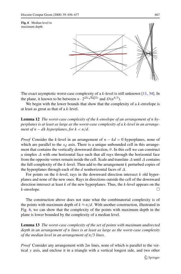
Fig. 6 Median level tomaximum depth

The exact asymptotic worst-case complexity of a k-level is still unknown [11, 34]. Inthe plane, it known to be between n · 2Ω(

√logn) and O(n4/3).

We begin with the lower bounds that show that the complexity of a k-envelope isat least as great as that of a k-level.

Lemma 12 The worst-case complexity of the k-envelope of an arrangement of n hy-perplanes is at least as large as the worst-case complexity of a k-level in an arrange-ment of n − dk hyperplanes, for k < n/d .

Proof Consider the k-level in an arrangement of n − kd > 0 hyperplanes, none ofwhich are parallel to the xd axis. There is a unique unbounded cell in this arrange-ment that contains the vertically downward direction, θ . In this cell we can constructa simplex Δ with one horizontal face such that all rays through the horizontal facefrom the opposite vertex remain inside the cell. Scale and translate Δ until Δ containsthe full complexity of the k-level. Then add to the arrangement k perturbed copies ofthe hyperplanes through each of the d nonhorizontal faces of Δ.

For points on the k-level, rays in the downward direction intersect k old hyper-planes and none of the new ones. Rays in directions outside the cell of the downwarddirection intersect at least k of the new hyperplanes. Thus, the k-level appears on thek-envelope. �

The construction above does not state what the combinatorial complexity is ofthe points with maximum depth of k ≈ n/d . With another construction, illustrated inFig. 6, we can show that the complexity of the points with maximum depth in theplane is lower bounded by the complexity of a median level.

Lemma 13 The worst-case complexity of the set of points with maximum undirecteddepth in an arrangement of n lines is at least as large as the worst-case complexityof the median level in an arrangement of n/3 lines.

Proof Consider any arrangement with 2m lines, none of which is parallel to the ver-tical y axis, and enclose it in a triangle with a vertical longest side, and two other


nearly vertical sides. Add 2m lines through the longest side and m through each ofthe others, then perturb the new lines to be in general position.

Unbounded cells in the original arrangement now have undirected depth at most2m by crossing only new lines. Bounded cells in the original arrangement also haveundirected depth at most 2m by crossing m old lines and m new with a near-verticalray. The former median level has undirected depth of exactly 2m, and thus contributespoints of maximum depth. �

4.3 Deepest Points in Nondegenerate Arrangements

We expand on the discussion given earlier in this section to characterize the whole setof maximum depth points in nondegenerate arrangements. As we just showed, thisset can have superlinear complexity.

Lemma 14 If the maximum cell depth is i, then the maximum depth points formeither

1. a single point of depth i + 2;2. a convex polygon whose vertices, edges, and interior all have depth i; or3. a single chain of segments and some isolated points of depth i + 1, where either

the single chain or the isolated points need not be present.1

Proof The first and second cases are discussed in Sect. 4.1; we establish the structureof the third by considering the configurations of Fig. 5 that give vertices and edgesof depth i + 1. If we consider the witness directions for cells of depth i − 1 adjacentto cells of depth i in these cases, and apply the Wedge lemma, we can make thefollowing observations.

In configuration 1I, there is a wedge defined by directions for the two cells ofdepth i − 1 that includes a ray on the line separating these two cells. In configuration1A, there are two such wedges. The Wedge lemma implies that cells in these wedgesare of depth at most i − 1. This immediately implies that all edges in the wedge havedepth at most i. In fact, vertices in the wedge also have depth at most i, since theonly way for a vertex to have depth i + 1 would be to have four incident cells ofdepth i − 1, but then i − 1 would be the maximum depth of a cell in the arrangement.

In configuration 1X, we consider two witness directions for the cells of depthi − 1, and let them define rays that originate at the intersection point of configuration1X. The rays define a wedge that contains one of the two incident cells of depth i.Translate the wedge slightly so that its apex is in the other cell of depth i. Cases (iv)and (v) of the Wedge lemma show that all cells and edges in the wedge have depth atmost i. There may be isolated vertices of depth i + 1 in the wedge.

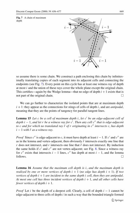
It is clear that configurations 1A and 1X give isolated vertices of depth i + 1, that1I gives the end of a chain of vertices and edges of depth i + 1, and that 1V gives themiddle of such a chain (see Fig. 7). We need to show that there is at most one chain,

1The conference version claimed that the chain has O(n) segments, but our proof of that claim turned outto be incorrect.


Fig. 7 A chain of maximumdepth

so assume there is some chain. We construct a path enclosing this chain by infinites-imally translating copies of each segment into its adjacent cells and connecting theendpoints (see Fig. 7). Every point on this cycle has at least one witness ray of depthat most i and the union of these rays cover the whole plane except the original chain.This certifies—again by the Wedge lemma—that no edge of depth i + 1 exists that isnot part of the original chain. �

We can go further to characterize the isolated points that are at maximum depthi + 1: they appear as the connections for stings of cells of depth i, and are antipodal,meaning that they are the points of tangency for parallel tangent lines.

Lemma 15 Let c be a cell of maximum depth i, let c′ be an edge-adjacent cell ofdepth i − 1, and let r be a witness ray for c′. Then any cell c′′ that is edge-adjacentto c and for which no translated ray r̄ of r originating in c′′ intersects c, has depthi − 1 with r̄ as a witness ray.

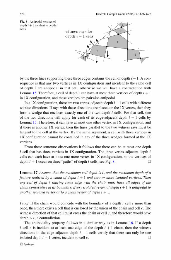
Proof Since c′′ is edge-adjacent to c, it must have depth at least i − 1. If c′ and c′′ areas in the lemma and vertex-adjacent, then obviously r̄ intersects exactly one line thatr does not intersect, and r intersects one line that r̄ does not intersect. By inductionthe same holds if c′ and c′′ are not vertex-adjacent; see Fig. 8. Since a witness rayfor c′′ exists that intersects i − 1 lines, c′′ has depth at most i − 1, and the lemmafollows. �

Lemma 16 Assume that the maximum cell depth is i, and the maximum depth isrealized by one or more vertices of depth i + 1 (no edge has depth i + 1). If twovertices of depth i + 1 are incident to the same depth i cell, then they are antipodal.At most one cell has three incident vertices of depth i + 1, and all other cells havefewer vertices of depth i + 1.

Proof Let i be the depth of a deepest cell. Clearly, a cell of depth i − 1 cannot beedge-adjacent to three cells of depth i in such a way that the bounded triangle formed


Fig. 8 Antipodal vertices ofdepth i + 1 incident to depth i

cells

by the three lines supporting these three edges contains the cell of depth i −1. A con-sequence is that any two vertices in 1X configuration and incident to the same cellof depth i are antipodal in that cell, otherwise we will have a contradiction withLemma 15. Therefore, a cell of depth i can have at most three vertices of depth i + 1in 1X configuration, and these vertices are pairwise antipodal.

In a 1X configuration, there are two vertex-adjacent depth i −1 cells with differentwitness directions. If rays with these directions are placed on the 1X vertex, then theyform a wedge that encloses exactly one of the two depth i cells. For that cell, oneof the two directions will apply for each of its edge-adjacent depth i − 1 cells byLemma 15. Therefore, it can have at most one other vertex in 1X configuration, andif there is another 1X vertex, then the lines parallel to the two witness rays must betangent to the cell at the vertex. By the same argument, a cell with three vertices in1X configuration cannot be contained in any of the three wedges formed at the 1Xvertices.

From these structure observations it follows that there can be at most one depthi cell that has three vertices in 1X configuration. The three vertex-adjacent depth i

cells can each have at most one more vertex in 1X configuration, so the vertices ofdepth i + 1 occur on three “paths” of depth i cells; see Fig. 8. �

Lemma 17 Assume that the maximum cell depth is i, and the maximum depth of afeature realized by a chain of depth i + 1 and zero or more isolated vertices. Thenany cell of depth i sharing some edge with the chain must have all edges of thechain consecutive in its boundary. Every isolated vertex of depth i + 1 is antipodal toanother isolated vertex or to a chain vertex of depth i + 1.

Proof If the chain would coincide with the boundary of a depth i cell c more thanonce, then there exists a cell that is enclosed by the union of the chain and cell c. Thewitness direction of that cell must cross the chain or cell c, and therefore would havedepth > i, a contradiction.

The antipodality property follows in a similar way as in Lemma 16. If a depthi cell c is incident to at least one edge of the depth i + 1 chain, then the witnessdirections in the edge-adjacent depth i − 1 cells certify that there can only be oneisolated depth i + 1 vertex incident to cell c. �


4.4 Output-Sensitive Construction for Maximum Depth in Nondegenerate PlanarArrangements

A dynamic convex hull maintenance algorithm, when applied to the duals of the lines,allows us to maintain a description of the current cell as we walk from cell to cell inthe arrangement. With the characterization of the points of maximum depth fromSect. 4.3, this allows us to compute a description of the maximum depth points in anoutput-sensitive manner.

Theorem 18 After O(n log2 n) preprocessing, the set of all edges and vertices atmaximum depth in an arrangement of lines in general position can be computed atthe cost of O(log3/2 n) time per feature.

Proof For the preprocessing, use the result of Theorem 10 to find a deepest cell. Buildthe tournament structure for this cell (Lemma 9). Let H be the set of half-planes withthe lines as bounding lines, such that the deepest cell that was found is

⋂h∈H h.

Dualize the lines bounding positive half-planes to points and build a lower convexhull maintenance structure for them. We choose the one of Chan [6], which allowsall necessary operations in O(log3/2 n) time. Similarly, build an upper convex hullmaintenance structure for the points dual to lines that bound negative half-planes.The convex hull maintenance structures allow us to do a search on the boundaryof a deepest cell. We can switch to an adjacent cell in O(log3/2 n) time by updat-ing all three data structures. Therefore, we can decide in O(log3/2 n) time what thedepth of an incident edge or vertex is, and also what the type of a vertex is. We canalso do linear programming queries (find extreme vertices for a direction) in cells ofthe arrangement in O(log3/2 n) time, which are the dual of vertical line intersectionqueries with the convex hull.

We note that our algorithm to find a deepest cell will find a cell of depth i thatis adjacent to the depth i + 1 chain, if it exists. Also, it will find the cell with threeincident antipodal vertices of depth i + 1, if such a cell exists. So we can determinein O(n log3/2 n) additional time whether case 3 of Lemma 14 applies, by inspectingthe whole boundary of the cell, or get the three depth i + 1 vertices. Furthermore,using the data structures, we can easily obtain the whole depth i + 1 chain in timeO(k log3/2 n) if it has k edges.

When we check any other depth i cell by continuing over a depth i+1 edge or overthe lines intersecting in a vertex in 1X configuration, we cannot examine the wholeboundary and achieve the claimed time bound. Instead we will perform a search inthe cell to find any other features of depth i + 1. This will be done using the witnessdirections of adjacent depth i − 1 cells (which was already suggested by the proof ofLemma 16).

Let v be a known depth i + 1 vertex of a cell c of depth i, and assume that itis isolated. Then v is incident to two depth i − 1 cells, and the rays with their wit-ness directions, when originating in v, form a wedge that contains c. If v is part ofthe depth i + 1 chain, then we get the witness directions at the most clockwise andcounterclockwise depth i + 1 vertices of the chain. When placed at these vertices, therays with the witness directions and the subchain together form an unbounded convex


Fig. 9 A depth i + 1 chain(fat), two depth i + 1 isolatedvertices, a cell c of depth i, andthe two witness directions (fatarrows) for the search illustrated

polygon that contains c. Figure 9 shows an example with two (dashed) rays and oneedge (fat) of the chain.

To find the at most one other vertex of depth i + 1—in 1X configuration—weperform a linear programming query with each of the two witness rays. If they findthe same vertex in c, then this vertex may be in 1X configuration, and the vertex-adjacent cell would then have depth i. We can test this using our data structures inO(log3/2 n) time. If they find different vertices, then the cell has no other depth i + 1vertices due to Lemma 15 and the fact that the initial witness rays form a wedge thatcontains the cell (when the rays are placed at the known depth i + 1 vertex). In casewe find another depth i + 1 vertex, the search proceeds in the vertex-adjacent depth i

cell with the same two witness rays.After processing all depth i cells we have found all depth i + 1 features in at most

O(log3/2 n) time per feature. �

It may be possible to use a more efficient dynamic convex hull maintenance struc-ture like the one of Brodal and Jacob [4], but it is unclear if all necessary operationsthat we need can be performed more efficiently using their data structure.

4.5 Depth of Vertices in Degenerate Arrangements

Efficiently finding a deepest vertex in a degenerate arrangement of lines appears tobe difficult. However, we can efficiently find a vertex whose depth is within a factorof (1 − o(1)) from the maximum depth.

Lemma 19 A point whose depth is at least (1 − log(logn)logn

) times the maximum can befound in O(n logn) time.

Proof First, compute the cell of maximum depth in the arrangement. Then, usingan algorithm of Guibas et al. [17], find all vertices V that are contained in at leastn

3 log(logn)logn

lines in O(n logn) time. There are at most O(logn

log(logn)) of these vertices,

and their depth can be tested in O(n) time each once the lines are sorted by slope.


Either a vertex of V has maximum depth, or, by Lemma 1, a point in the cell ofmaximum depth is less than n

3 log(logn)logn

from the true maximum value. Since Amentaet al. proved in [3] that the maximum value is at least �n/3� we therefore have anapproximation factor of at least (1 − log(logn)

logn). �

One heuristic that involves less programming is to symbolically perturb the linesof the arrangement to simulate general position and compute the cell of maximumdepth. In the original arrangement this cell may correspond to a vertex, in which casewe evaluate the depth of this vertex, or to a cell, in which case we construct the celland evaluate the depth of all of its vertices. From the Wedge lemma it can be seenthat the actual maximum depth will be at most double the computed depth.

5 Computing Depth in Higher Dimensions

For three and higher dimensions, Corollary 4 states that we can compute the maxi-mum depth in O(nd) time and space by evaluating depth at all cells and vertices ofan arrangement. It is challenging to develop more efficient algorithms.

5.1 The Wedge Lemma Cannot Extend to 3

The solution for the planar case was based on the Wedge lemma, which allowedus to argue that certain regions of the plane could not contain a cell of maximumdepth. When thinking about the extension to three dimensions, one would first try togeneralize the Wedge lemma: that for a point p whose depth i is witnessed by threevectors �u, �v, and �w, the cone defined by �u, �v, and �w does not contain a cell of depthgreater than i. The following construction shows that this is not true.

Let point p be the origin of the coordinate system. We construct an arrangementof 15 planes such that the positive x-axis, the positive y-axis, and the positive z-axiseach witness that depth(p) = 2, the point q = (2,2,2) will have depth(q) = 3.

There are six planes that intersect the positive octant: Planes x = 4, y = 4, andz = 4 are parallel to the coordinate planes. Planes 5 = −x −y +5z, 5 = −x +5y − z,and 5 = 5x − y − z pass through a common point (5/3,5/3,5/3), and each intersectone of the positive coordinate axes. Note that the first intersects the z axis at (0,0,1)

and the x and y axes at (−5,0,0) and (0,−5,0). Note that if the coordinate frameis translated from the origin to q = (2,2,2), then each positive axis intersects threeof these six planes, which already shows that the argument used to prove the two-dimensional Wedge lemma does not hold in the three-dimensional case.

The remaining nine planes are chosen to make sure that only directions in ornear the positive octant can give depth counts below three for all cells in the posi-tive octant. They are perturbed versions of x = −1, x = −2, x = −3 and similarly,y, z = −1,−2,−3. The perturbations are such that none of the planes intersect thepositive octant. The common intersection of the half-spaces bounded by these planesand containing the origin can be seen as the perturbed positive octant. These makesure that for any point in the positive octant, and any direction outside the positiveoctant by a small angle, the depth count in that direction will be at least three.


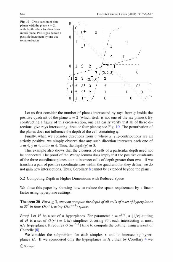
Fig. 10 Cross-section of nineplanes with the plane x = 2,with depth values for directionsin this plane. Plus signs denote apossible increment by one dueto perturbation

Let us first consider the number of planes intersected by rays from q inside thepositive quadrant of the plane x = 2 (which itself is not one of the six planes). Byconstructing a figure of this cross-section, one can easily verify that all of these di-rections give rays intersecting three or four planes; see Fig. 10. The perturbation ofthe planes does not influence the depth of the cell containing q .

Finally, when we consider directions from q where x, y, z-contributions are allstrictly positive, we simply observe that any such direction intersects each one ofx = 4, y = 4, and z = 4. Thus, the depth(q) = 3.

This example also shows that the closures of cells of a particular depth need notbe connected. The proof of the Wedge lemma does imply that the positive quadrantsof the three coordinate planes do not intersect cells of depth greater than two—if wetranslate a pair of positive coordinate axes within the quadrant that they define, we donot gain new intersections. Thus, Corollary 8 cannot be extended beyond the plane.

5.2 Computing Depth in Higher Dimensions with Reduced Space

We close this paper by showing how to reduce the space requirement by a linearfactor using hyperplane cuttings.

Theorem 20 For d ≥ 3, one can compute the depth of all cells of a set of hyperplanesin d in time O(nd), using O(nd−1) space.

Proof Let H be a set of n hyperplanes. For parameter r = n1/d , a (1/r)-cuttingof H is a set of O(rd) = O(n) simplices covering d , each intersecting at mostn/r hyperplanes. It requires O(nrd−1) time to compute the cutting, using a result ofChazelle [8].

We consider the subproblem for each simplex τ and its intersecting hyper-planes Hτ . If we considered only the hyperplanes in Hτ , then by Corollary 4 we


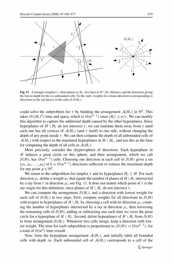
Fig. 11 A triangle (simplex) τ , three planes in Hτ , five lines in H \Hτ (thicker), and the directions givingthe lowest depth for the six unbounded cells. To the right, weights for certain directions (corresponding todirections in the left figure) in the cells of S(Hτ )

could solve the subproblem for τ by building the arrangement A(Hτ ) in d . Thistakes O(|Hτ |d) time and space, which is O(nd−1) since |Hτ | ≤ n/r . We can modifythis algorithm to capture the additional depth caused by the other hyperplanes. Sincehyperplanes of H \ Hτ do not intersect τ , we can translate them away from τ untileach one has all vertices of A(Hτ ) (and τ itself) to one side, without changing thedepth of any point inside τ . We can then compute the depth of all unbounded cells ofA(Hτ ) with respect to the translated hyperplanes in H \ Hτ , and use this as the basefor computing the depth of all cells in A(Hτ ).

More precisely, consider the (hyper)sphere of directions. Each hyperplane inH induces a great circle on this sphere, and their arrangement, which we callS(H), has O(nd−1) cells. Choosing one direction in each cell of S(H) gives a set{ρ1, ρ2, . . . , ρk} of k = O(nd−1) directions sufficient to witness the maximum depthfor any point p ∈ d .

We return to the subproblem for simplex τ and its hyperplanes Hτ ⊂ H . For eachdirection ρi , define a weight wi that equals the number of planes of H \Hτ intersectedby a ray from τ in direction ρi ; see Fig. 11. It does not matter which point of τ is theray origin for this definition, since planes of H \ Hτ do not intersect τ .

We can compute the arrangement S(Hτ ), and a direction with lowest weight foreach cell of S(Hτ ) in two steps. First, compute weights for all directions in S(H)

with respect to hyperplanes of H \Hτ by choosing a cell with its direction ρi , count-ing the number of hyperplanes intersected by a ray in direction ρi , then traversingthe remaining cells of S(H), adding or subtracting one each time we cross the greatcircle for a hyperplane of H \ Hτ . Second, delete hyperplanes of H \ Hτ from S(H)

to form arrangement S(Hτ ). Whenever two cells merge, keep a direction with low-est weight. The time for each subproblem is proportional to |S(H)| = O(nd−1), fora total of O(nd) time overall.

Now, form the hyperplane arrangement A(Hτ ), and initially label all boundedcells with depth ∞. Each unbounded cell of A(Hτ ) corresponds to a cell of the


spherical arrangement S(Hτ ); label it with the corresponding weight and direction.The minimum assigned depth is correct, so we can perform the loop as before: fori = 1, 2, . . . , n, all cells with label i − 1 cause their adjacent, higher-labeled cellsto be relabeled i. This takes O(nd−1) time and space for each simplex τ , leading toa total time of O(nd). �

6 Conclusions and Open Problems

This paper presented an O(n log2 n) time algorithm for computing a point with max-imum regression depth in the plane. Langerman and Steiger used our algorithm asa basis for their improved O(n logn) time algorithm [21]. We also gave an O(nd)

time, O(nd−1) space algorithm for maximum regression depth in higher dimensionsand various other results.

The most interesting open problems that remain are a more efficient algorithmfor computing regression depth in higher dimensions, and good approximation algo-rithms in the plane and higher dimensions.

Acknowledgements J. Mitchell and M. Sharir thank E. Arkin and S. Har-Peled for several helpfuldiscussions and suggestions. We also thank an anonymous referee for useful comments.

Open Access This article is distributed under the terms of the Creative Commons Attribution Noncom-mercial License which permits any noncommercial use, distribution, and reproduction in any medium,provided the original author(s) and source are credited.

References

1. Aelst, S.V., Rousseeuw, P.J.: Robustness of deepest regression. J. Multivar. Anal. 73, 82–106 (2000)2. Aelst, S.V., Rousseeuw, P.J., Hubert, M., Struyf, A.: The deepest regression method. J. Multivar. Anal.

81(1), 138–166 (2002)3. Amenta, N., Bern, M., Eppstein, D., Teng, S.-H.: Regression depth and center points. Discrete Com-

put. Geom. 23, 305–323 (2000)4. Brodal, G.S., Jacob, R.: Dynamic planar convex hull. In: Proc. 43rd Symposium on Foundations of

Computer Science (FOCS), pp. 617–626 (2002)5. Brönnimann, H., Chazelle, B.: Optimal slope selection via cuttings. Comput. Geom. Theory Appl.

10(1), 23–29 (1998)6. Chan, T.M.: Dynamic planar convex hull operations in near-logarithmic amortized time. J. ACM

48(1), 1–12 (2001)7. Chan, T.M.: An optimal randomized algorithm for maximum turkey depth. In: Proc. 15th ACM-SIAM

Symposium on Discrete Algorithms (SODA), pp. 430–436 (2004)8. Chazelle, B.: Cutting hyperplanes for divide-and-conquer. Discrete Comput. Geom. 9(2), 145–158

(1993)9. Chazelle, B., Preparata, F.P.: Halfspace range search: An algorithmic application of k-sets. Discrete

Comput. Geom. 1, 83–93 (1986)10. Cole, R., Salowe, J., Steiger, W., Szemerédi, E.: An optimal-time algorithm for slope selection. SIAM

J. Comput. 18(4), 792–810 (1989)11. Dey, T.K.: Improved bounds on planar k-sets and related problems. Discrete Comput. Geom. 19,

373–382 (1998)12. Dillencourt, M.B., Mount, D.M., Netanyahu, N.S.: A randomized algorithm for slope selection. Int.

J. Comput. Geom. Appl. 2, 1–27 (1992)13. Edelsbrunner, H.: Algorithms in Combinatorial Geometry. Springer, New York (1987)14. Edelsbrunner, H., O’Rourke, J., Seidel, R.: Constructing arrangements of lines and hyperplanes with

applications. SIAM J. Comput 15, 341–363 (1986)


15. Edelsbrunner, H., Seidel, R., Sharir, M.: On the zone theorem for hyperplane arrangements. SIAM J.Comput. 22(2), 418–429 (1993)

16. Eu, D., Guévremont, E., Toussaint, G.T.: On envelopes of arrangements of lines. J. Algorithms 21,111–148 (1996)

17. Guibas, L.J., Overmars, M.H., Robert, J.-M.: The exact fitting problem for points. Comput. Geom.Theory Appl. 6, 215–230 (1996)

18. Hubert, M., Rousseeuw, P.J.: The catline for deep regression. J. Multivar. Anal. 66, 270–296 (1998)19. Katz, M.J., Sharir, M.: Optimal slope selection via expanders. Inf. Process. Lett. 47, 115–122 (1993)20. Keil, M.: A simple algorithm for determining the envelope of a set of lines. Inf. Process. Lett. 39,

121–124 (1991)21. Langerman, S., Steiger, W.: The complexity of hyperplane depth in the plane. Discrete Comput.

Geom. 30(2), 299–309 (2003)22. Matoušek, J.: Randomized optimal algorithm for slope selection. Inf. Process. Lett. 39, 183–187

(1991)23. Peck, G.W.: On k-sets in the plane. Discrete Math. 56, 73–74 (1985)24. Rousseeuw, P.J., Aelst, S.V., Hubert, M.: Regression depth: Rejoinder. J. Am. Stat. Assoc. 94, 419–

433 (1999)25. Rousseeuw, P.J., Hubert, M.: Depth in an arrangement of hyperplanes. Discrete Comput. Geom. 22,

167–176 (1999)26. Rousseeuw, P.J., Hubert, M.: Regression depth. J. Am. Stat. Assoc. 94, 388–402 (1999)27. Rousseeuw, P.J., Ruts, I.: Constructing the bivariate Tukey median. Stat. Sin. 8, 827–839 (1998)28. Rousseeuw, P.J., Struyf, A.: Computing location depth and regression depth in higher dimensions.

Stat. Comput. 8, 193–203 (1998)29. Rousseeuw, P.J., Struyf, A.: Computation of robust statistics: depth, median, and related measures.

In: Goodman, J.E., O’Rourke, J. (eds.) The Handbook of Discrete and Computational Geometry, 2ndedn., pp. 1279–1292. Chapman & Hall/CRC, Boca Raton (2004)

30. Ruts, I., Rousseeuw, P.J.: Computing depth contours of bivariate point clouds. Comput. Stat. DataAnal. 23, 153–168 (1996)

31. Sharir, M.: k-sets and random hulls. Combinatorica 13, 483–495 (1993)32. Struyf, A., Rousseeuw, P.J.: Halfspace depth and regression depth characterize the empirical distribu-

tion. J. Multivar. Anal. 69, 135–153 (1999)33. Struyf, A., Rousseeuw, P.J.: High-dimensional computation of the deepest location. Comput. Stat.

Data Anal. 34, 415–426 (2000)34. Tóth, G.: Point sets with many k-sets. Discrete Comput. Geom. 26, 187–194 (2001)

Efﬁcient Algorithms for Maximum Regression … Comput Geom ... Efﬁcient Algorithms for Maximum...

Documents

Transcript of Efﬁcient Algorithms for Maximum Regression … Comput Geom ... Efﬁcient Algorithms for Maximum...