EEM561MachineVision Week6: … 561/icerik/EEM561_7.… · Spring2015 ’ ’ Instructor ......

EEM 561 Machine Vision

Week 6 : Scale Invariant Detec:on and Robust Fi@ng

Spring 2015

Instructor: Ha5ce Çınar Akakın, Ph.D. [email protected]

Anadolu University

2

Harris corner detector algorithm • Compute image gradients Ix Iy for all pixels •  For each pixel

•  Compute by looping over neighbors x,y

•  compute

•  Find points with large corner response func5on R (R > threshold)

•  Take the points of locally maximum R as the detected feature points (ie, pixels where R is bigger than for all the 4 or 8 neighbors).

hTp://www.wisdom.weizmann.ac.il/~deniss/vision_spring04/files/InvariantFeatures.ppt Darya Frolova, Denis Simakov The Weizmann Ins5tute of Science

Harris Detector: Invariance Proper:es • Rota5on

Ellipse rotates but its shape (i.e. eigenvalues) remains the same

Corner response is invariant to image rota5on

Harris Detector: Invariance Proper:es • Affine intensity change: I → aI + b

ü  Only deriva5ves are used => invariance to intensity shi_ I → I + b

ü  Intensity scale: I → a I

R

x (image coordinate)

threshold

R

x (image coordinate)

Par$ally invariant to affine intensity change

Harris Detector: Some Proper:es • Not invariant to image scale!

All points will be classified as edges

Corner !


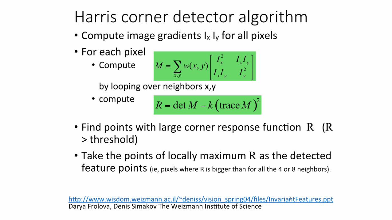
Harris Detector: Some Proper:es • Quality of Harris detector for different scale changes Repeatability rate:

# correspondences # possible correspondences

C.Schmid et.al. “Evalua5on of Interest Point Detectors”. IJCV 2000


Source: A. Torralbo

Scale Invariant Detec:on • Consider regions (e.g. circles) of different sizes around a point

• Regions of corresponding sizes will look the same in both images

The features look the same to these two operators.

hTp://www.wisdom.weizmann.ac.il/~deniss/vision_spring04/files/InvariantFeatures.ppt Darya Frolova, Denis Simakov The Weizmann Ins5tute of Science Source: A. Torralbo

Scale Invariant Detec:on •  The problem: how do we choose corresponding circles independently in each image?

• Do objects in the image have a characteris5c scale that we can iden5fy?


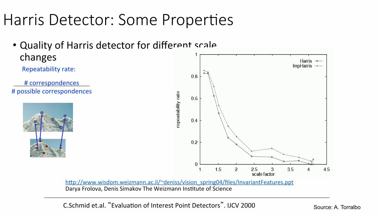
Scale Invariant Detec:on •  Solu5on:

•  Design a func5on on the region (circle), which is “scale invariant” (the same for corresponding regions, even if they are at different scales) Example: average intensity. For corresponding regions (even of

different sizes) it will be the same.

scale = 1/2

–  For a point in one image, we can consider it as a function of region size (circle radius)

f

region size

Image 1 f

region size

Image 2

Source: A. Torralbo

Scale Invariant Detec:on • Common approach:

Take a local maximum of this function

Observation: region size, for which the maximum is achieved, should be invariant to image scale.

scale = 1/2

f

region size

Image 1 f

region size

Image 2

s1 s2

Important: this scale invariant region size is found in each image independently!

Source: A. Torralbo

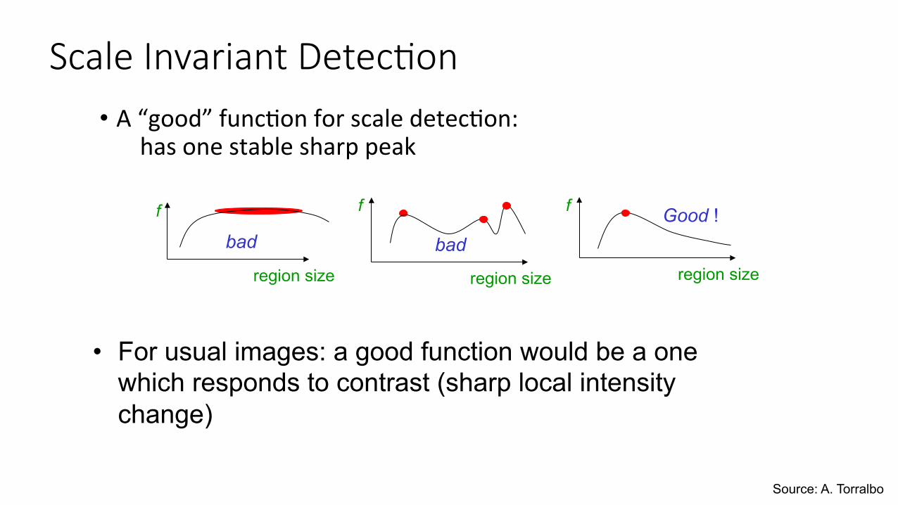
Scale Invariant Detec:on • A “good” func5on for scale detec5on: has one stable sharp peak

f

region size

bad

f

region size

bad

f

region size

Good !

•  For usual images: a good function would be a one which responds to contrast (sharp local intensity change)

Source: A. Torralbo

Detection over scale Requires a method to repeatably select points in location and scale: •  The only reasonable scale-‐space kernel is a Gaussian (Koenderink, 1984; Lindeberg, 1994)

•  An efficient choice is to detect peaks in the difference of Gaussian pyramid (Burt & Adelson, 1983; Crowley & Parker, 1984 – but examining more scales)

•  Difference-‐of-‐Gaussian with constant ra5o of scales is a close approxima5on to Lindeberg’s scale-‐normalized Laplacian (can be shown from the heat diffusion equa5on)

Source: A. Torralbo

Scale Invariant Detec:on •  Func5ons for determining scale

Kernels:

where Gaussian

Note: both kernels are invariant to scale and rotation

(Laplacian: 2nd deriva5ve of Gaussian)

(Difference of Gaussians)


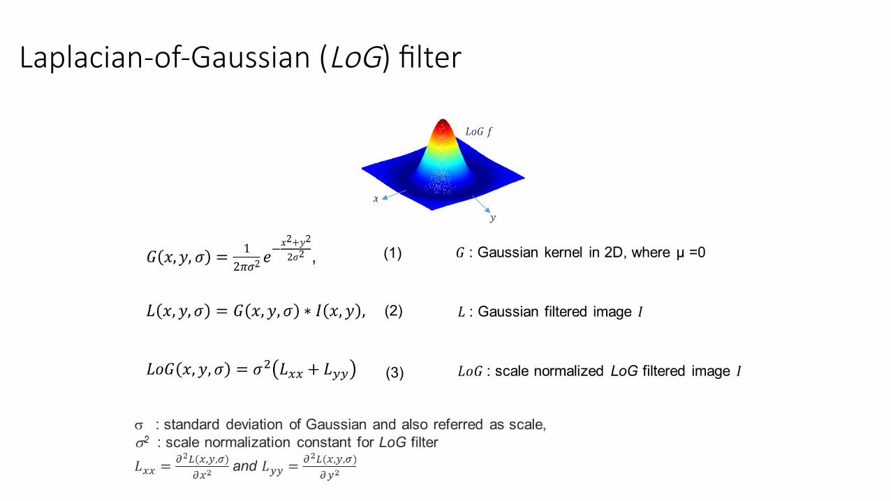
(1)

(2)

(3)

Laplacian-‐of-‐Gaussian (LoG) filter

r=40

Scale selec:on

d

d = 80 r = 40

{ 92.9 109.1 149.8 178.2 186.2 181.9 171.4 158.5 }

r

Characteris:c scale

• We define the characteris5c scale as the scale that produces peak of Laplacian response

characteris5c scale

T. Lindeberg (1998). "Feature detec5on with automa5c scale selec5on." Interna$onal Journal of Computer Vision 30 (2): pp 77-‐-‐116.

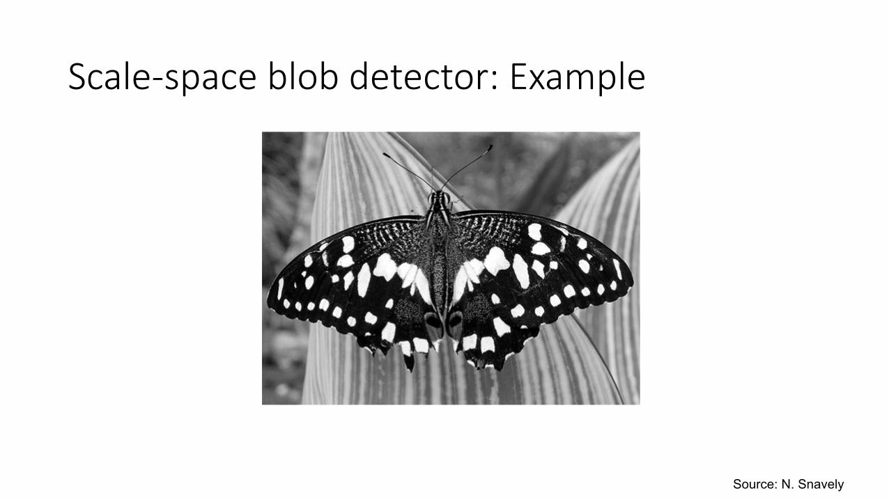
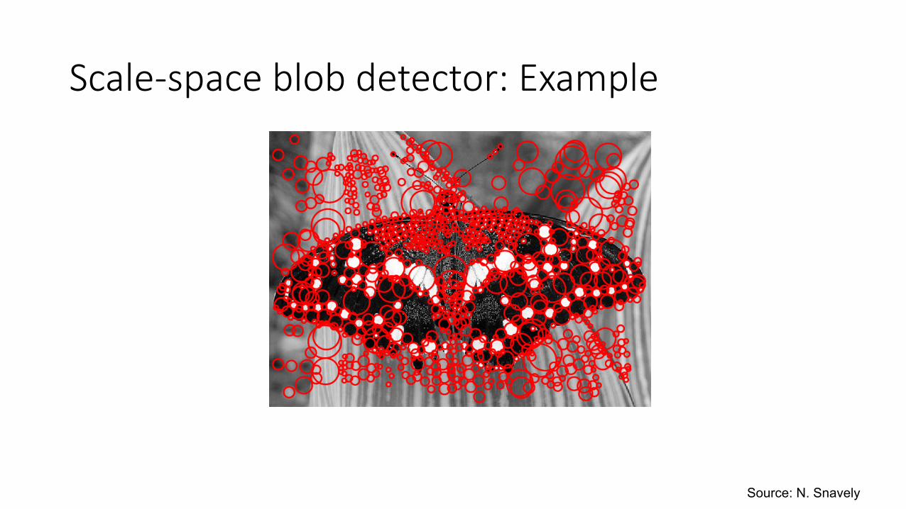
Scale-‐space blob detector: Example

Source: N. Snavely

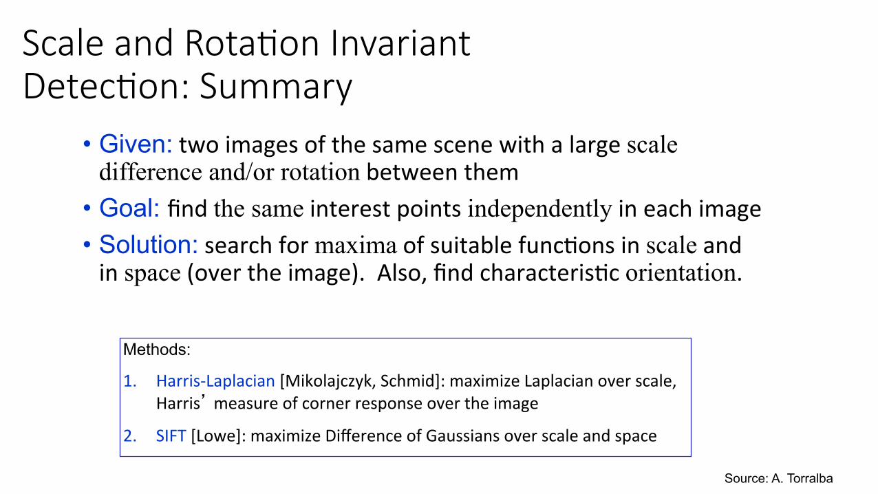
Scale and Rota:on Invariant Detec:on: Summary

• Given: two images of the same scene with a large scale difference and/or rotation between them

• Goal: find the same interest points independently in each image • Solution: search for maxima of suitable func5ons in scale and in space (over the image). Also, find characteris5c orientation.

Methods:

1.  Harris-‐Laplacian [Mikolajczyk, Schmid]: maximize Laplacian over scale, Harris’ measure of corner response over the image

2.  SIFT [Lowe]: maximize Difference of Gaussians over scale and space

Source: A. Torralba

Difference-‐of-‐Gaussian (DoG)

K. Grauman, B. Leibe

-‐ =

DoG – Efficient Computa:on • Computa5on in Gaussian scale pyramid


σ

Original image 41

2=σ

Sampling with step σ4 =2

σ

σ

σ

Find local maxima in posi:on-‐scale space of Difference-‐of-‐Gaussian


)()( σσ yyxx LL +

σ

σ2

σ3

σ4

σ5

⇒ List of (x, y, s)

Results: Difference-‐of-‐Gaussian


Harris-‐Laplace [Mikolajczyk ‘01] 1.  Ini5aliza5on: Mul5scale Harris corner detec5on

σ

σ2

σ3

σ4

Compu+ng Harris func+on Detec+ng local maxima

Harris-‐Laplace [Mikolajczyk ‘01]

1.  Ini5aliza5on: Mul5scale Harris corner detec5on 2.  Scale selec5on based on Laplacian


Harris points

Harris-‐Laplace points

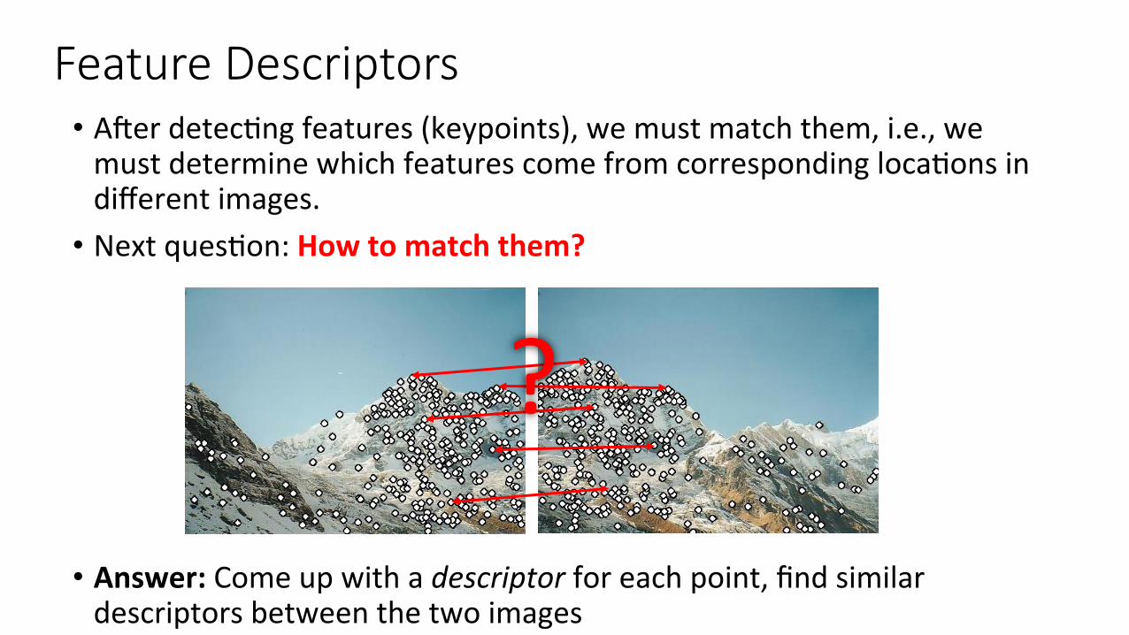
Feature Descriptors • A_er detec5ng features (keypoints), we must match them, i.e., we must determine which features come from corresponding loca5ons in different images.

• Next ques5on: How to match them?

• Answer: Come up with a descriptor for each point, find similar descriptors between the two images

?

Feature descriptors We know how to detect good points Next ques5on: How to match them? Lots of possibili5es (this is a popular research area)

•  Simple op5on: match square windows around the point •  State of the art approach: SIFT

•  David Lowe, UBC hTp://www.cs.ubc.ca/~lowe/keypoints/

?

T. Tuytelaars, B. Leibe

Orienta:on Normaliza:on

• Compute orienta5on histogram •  Select dominant orienta5on • Normalize: rotate to fixed orienta5on

0 2 π

[Lowe, SIFT, 1999]

CVPR 2003 Tutorial Recognition and Matching Based on Local Invariant Features

David Lowe Computer Science Department University of Bri5sh Columbia

hTp://www.cs.ubc.ca/~lowe/papers/ijcv04.pdf

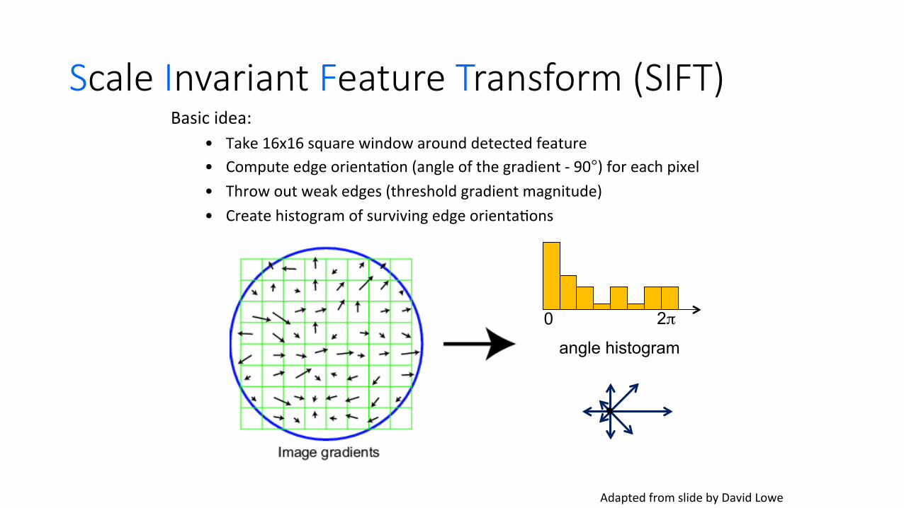
Basic idea: •  Take 16x16 square window around detected feature •  Compute edge orienta5on (angle of the gradient -‐ 90°) for each pixel •  Throw out weak edges (threshold gradient magnitude) •  Create histogram of surviving edge orienta5ons

Scale Invariant Feature Transform (SIFT)

Adapted from slide by David Lowe

0 2π

angle histogram

SIFT descriptor Full version

•  Divide the 16x16 window into a 4x4 grid of cells (2x2 case shown below) •  Compute an orienta5on histogram for each cell •  16 cells * 8 orienta5ons = 128 dimensional descriptor

Adapted from slide by David Lowe

SIFT vector forma5on

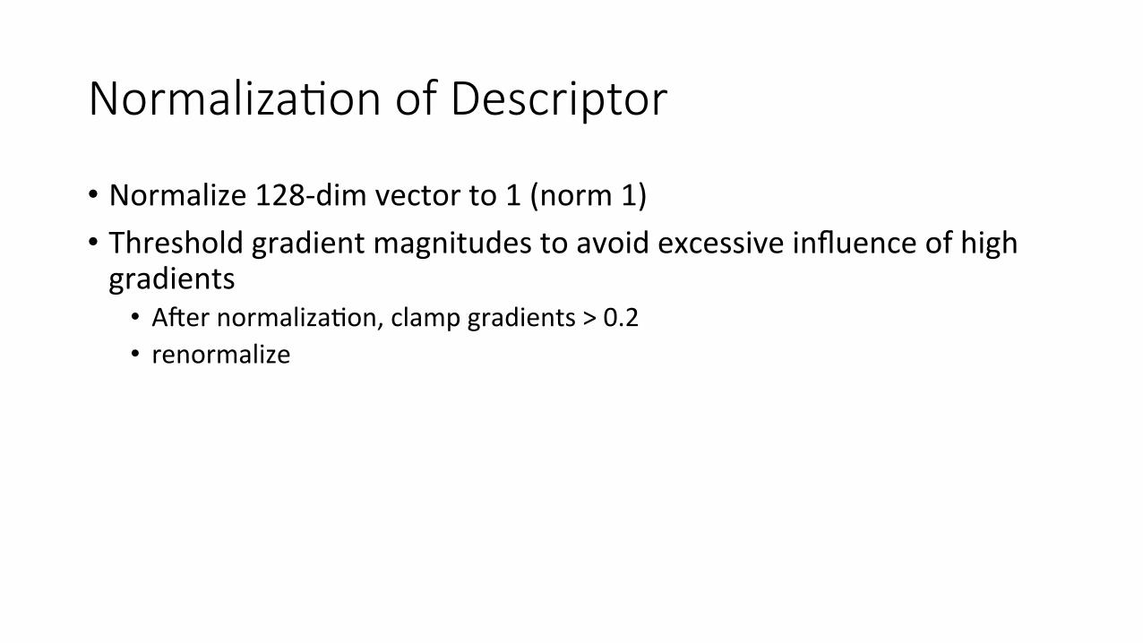
Normaliza:on of Descriptor

• Normalize 128-‐dim vector to 1 (norm 1) •  Threshold gradient magnitudes to avoid excessive influence of high gradients

•  A_er normaliza5on, clamp gradients > 0.2 •  renormalize

35

Tuning and evaluating the SIFT descriptors

Database images were subjected to rota5on, scaling, affine stretch, brightness and contrast changes, and added noise. Feature point detectors and descriptors were compared before and a_er the distor5ons, and evaluated for:

•  Sensi5vity to number of histogram orienta5ons and subregions. •  Stability to noise. •  Stability to affine change. •  Feature dis5nc5veness

35 Source: A. Torralba

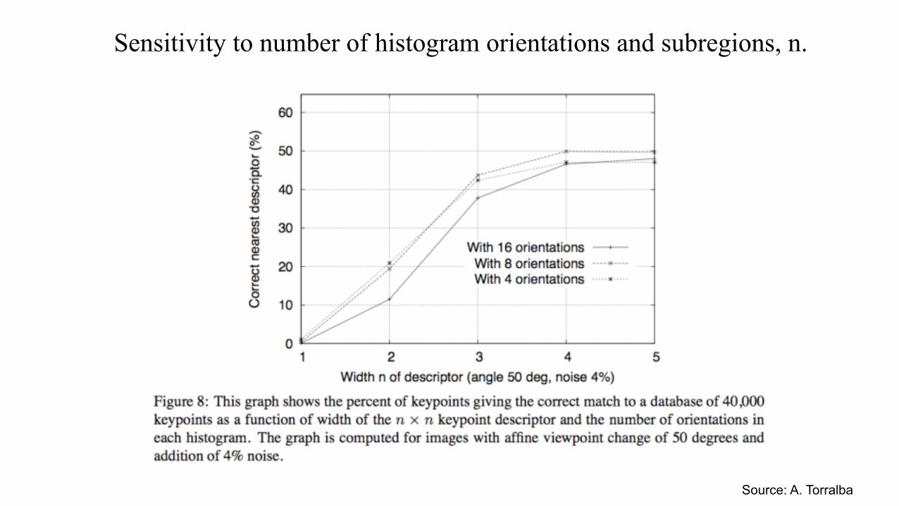
Sensitivity to number of histogram orientations and subregions, n.

Source: A. Torralba

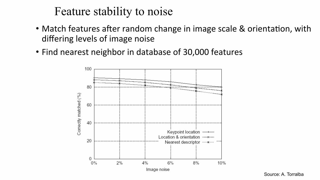
Feature stability to noise • Match features a_er random change in image scale & orienta5on, with differing levels of image noise

•  Find nearest neighbor in database of 30,000 features

Source: A. Torralba

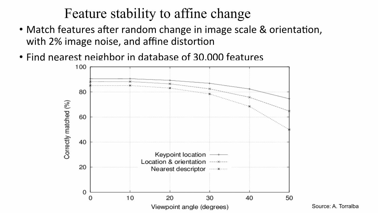
Feature stability to affine change • Match features a_er random change in image scale & orienta5on, with 2% image noise, and affine distor5on

•  Find nearest neighbor in database of 30,000 features

Source: A. Torralba

Invariance vs. discriminability

•  Invariance: •  Descriptor shouldn’t change even if image is transformed

• Discriminability: •  Descriptor should be highly unique for each point

Image transforma:ons • Geometric

Rota+on

Scale

• Photometric Intensity change

Source: N. Snavely

Invariance

Suppose we are comparing two images I1 and I2 •  I2 may be a transformed version of I1 • What kinds of transforma5ons are we likely to encounter in prac5ce?

Source: N. Snavely

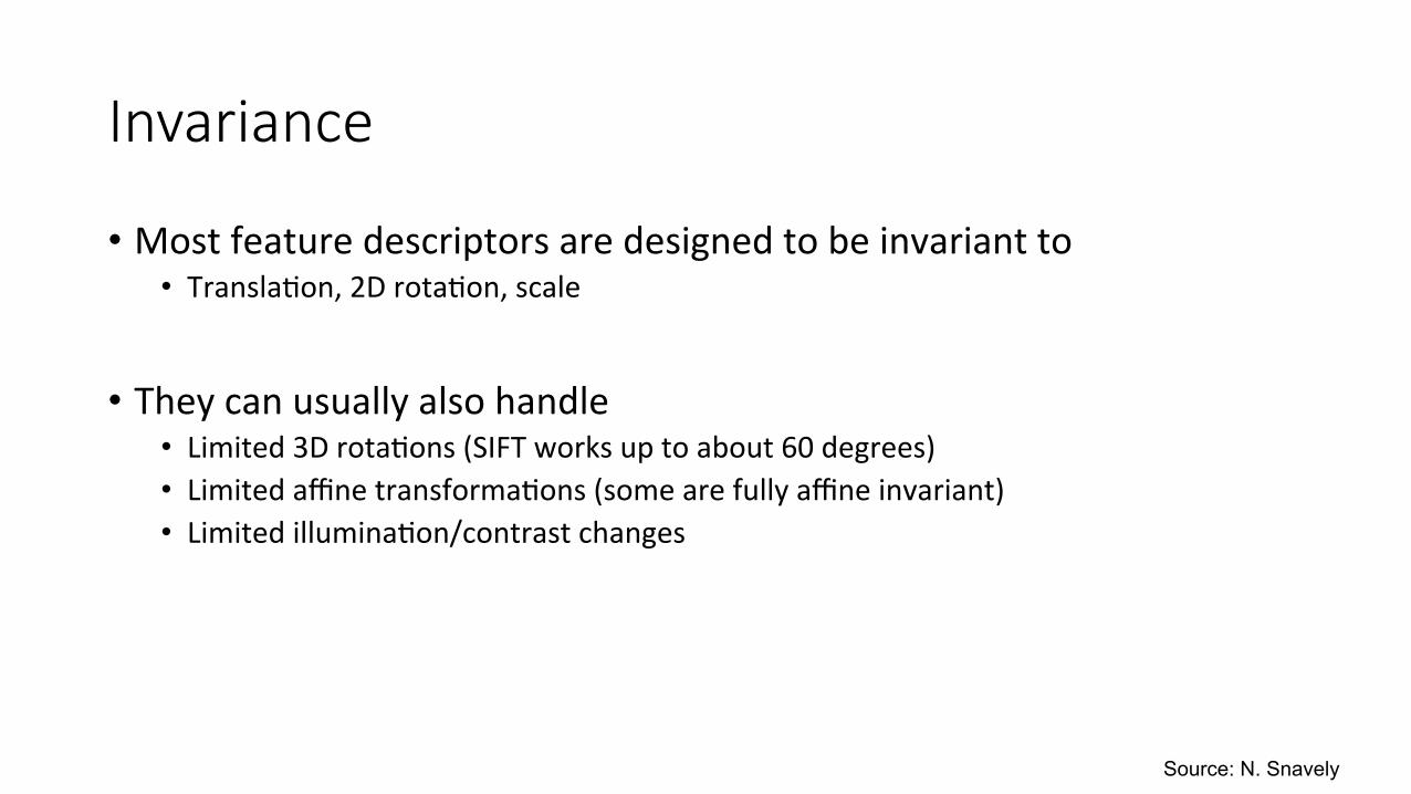
Invariance

• Most feature descriptors are designed to be invariant to •  Transla5on, 2D rota5on, scale

•  They can usually also handle •  Limited 3D rota5ons (SIFT works up to about 60 degrees) •  Limited affine transforma5ons (some are fully affine invariant) •  Limited illumina5on/contrast changes

Source: N. Snavely

Application of invariant local features to object (instance) recognition.

Image content is transformed into local feature coordinates that are invariant to transla5on, rota5on, scale, and other imaging parameters

SIFT Features Source: A. Torralba

•  Find dominant orienta5on of the image patch •  This is given by xmax, the eigenvector of H corresponding to λmax (the larger eigenvalue) •  Rotate the patch according to this angle

Rota:on invariance for feature descriptors

Figure by MaThew Brown Source: N. Snavely

Take 40x40 square window around detected feature

•  Scale to 1/5 size (using prefiltering)

•  Rotate to horizontal •  Sample 8x8 square window centered at feature

•  Intensity normalize the window by subtrac5ng the mean, dividing by the standard devia5on in the window

CSE 576: Computer Vision

Mul:scale Oriented PatcheS descriptor

8 pixels 40 pixels

Adapted from slide by MaThew Brown

Local Descriptors: SURF


•  Fast approxima+on of SIFT idea Ø  Efficient computa+on by 2D box filters &

integral images ⇒ 6 +mes faster than SIFT

Ø  Equivalent quality for object iden+fica+on

[Bay, ECCV’06], [Cornelis, CVGPU’08]

•  GPU implementa+on available Ø  Feature extrac+on @ 200Hz

(detector + descriptor, 640×480 img) Ø  http://www.vision.ee.ethz.ch/~surf

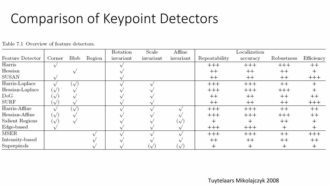
Comparison of Keypoint Detectors

Tuytelaars Mikolajczyk 2008

Things to remember

• Keypoint detec5on: repeatable and dis5nc5ve

•  Corners, blobs, stable regions •  Harris, DoG

• Descriptors: robust and selec5ve •  spa5al histograms of orienta5on •  SIFT

Source: J. Hays

SIFT features impact

A good SIFT features tutorial:

hTp://www.cs.toronto.edu/~jepson/csc2503/tutSIFT04.pdf

By Estrada, Jepson, and Fleet.

The original SIFT paper: hTp://www.cs.ubc.ca/~lowe/papers/ijcv04.pdf

SIFT feature paper citations: Dis5nc5ve image features from scale-‐invariant keypoints, DG Lowe -‐ Interna5onal journal of

computer vision, 2004 -‐ Springer Interna5onal Journal of Computer Vision 60(2), 91–110, 2004 cс 2004 Kluwer Academic Publishers. Computer Science Department, University of Bri5sh Columbia ...Cited by 16232 (google)

Source: A. Torralba

Now we have

• Well-‐localized feature points • Dis5nc5ve descriptor

• Now we need to •  match pairs of feature points in different images •  Robustly compute homographies (in the presence of errors/outliers)

EEM561MachineVision Week6: … 561/icerik/EEM561_7.… · Spring2015 ’ ’ Instructor ......

Documents

Transcript of EEM561MachineVision Week6: … 561/icerik/EEM561_7.… · Spring2015 ’ ’ Instructor ......