CPU Caches and Why You Care - Scott Meyers Caches and Why You Care CPU Caches Three common types:
date post
20-Dec-2015Category
view
220download
1
EECS 252 Graduate Computer Architecture
Lecture 2
0 Review of Instruction Sets, Pipelines,
and Caches January 26th, 2009
John KubiatowiczElectrical Engineering and Computer Sciences
University of California, Berkeley
http://www.eecs.berkeley.edu/~kubitron/cs252

1/26/2009 CS252-S09, Lecture 02 2
Review: Moore’s Law
• “Cramming More Components onto Integrated Circuits”– Gordon Moore, Electronics, 1965
• # on transistors on cost-effective integrated circuit double every 18 months
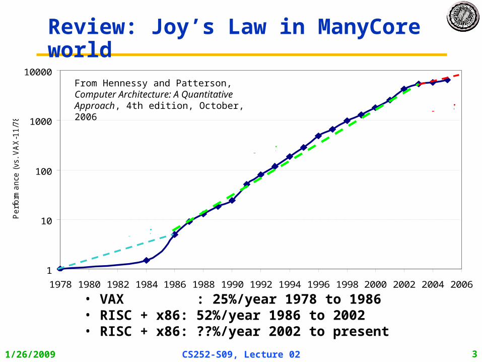
1/26/2009 CS252-S09, Lecture 02 3
1
10
100
1000
10000
1978 1980 1982 1984 1986 1988 1990 1992 1994 1996 1998 2000 2002 2004 2006
Pe
rfo
rma
nce
(vs
. V
AX
-11
/78
0)
25%/year
52%/year
??%/year
Review: Joy’s Law in ManyCore world
• VAX : 25%/year 1978 to 1986• RISC + x86: 52%/year 1986 to 2002• RISC + x86: ??%/year 2002 to present
From Hennessy and Patterson, Computer Architecture: A Quantitative Approach, 4th edition, October, 2006

1/26/2009 CS252-S09, Lecture 02 4
“Bell’s Law” – new class per decade
year
log
(p
eo
ple
pe
r c
om
pu
ter)
streaming informationto/from physical world
Number CrunchingData Storage
productivityinteractive
• Enabled by technological opportunities
• Smaller, more numerous and more intimately connected
• Brings in a new kind of application
• Used in many ways not previously imagined

1/26/2009 CS252-S09, Lecture 02 5
Today: Quick review of everything you should
have learned
0
( A countably-infinite set of computer architecture concepts )

1/26/2009 CS252-S09, Lecture 02 6
Metrics used to Compare Designs
• Cost– Die cost and system cost
• Execution Time– average and worst-case– Latency vs. Throughput
• Energy and Power– Also peak power and peak switching current
• Reliability– Resiliency to electrical noise, part failure– Robustness to bad software, operator error
• Maintainability– System administration costs
• Compatibility– Software costs dominate
1/26/2009 CS252-S09, Lecture 02 7
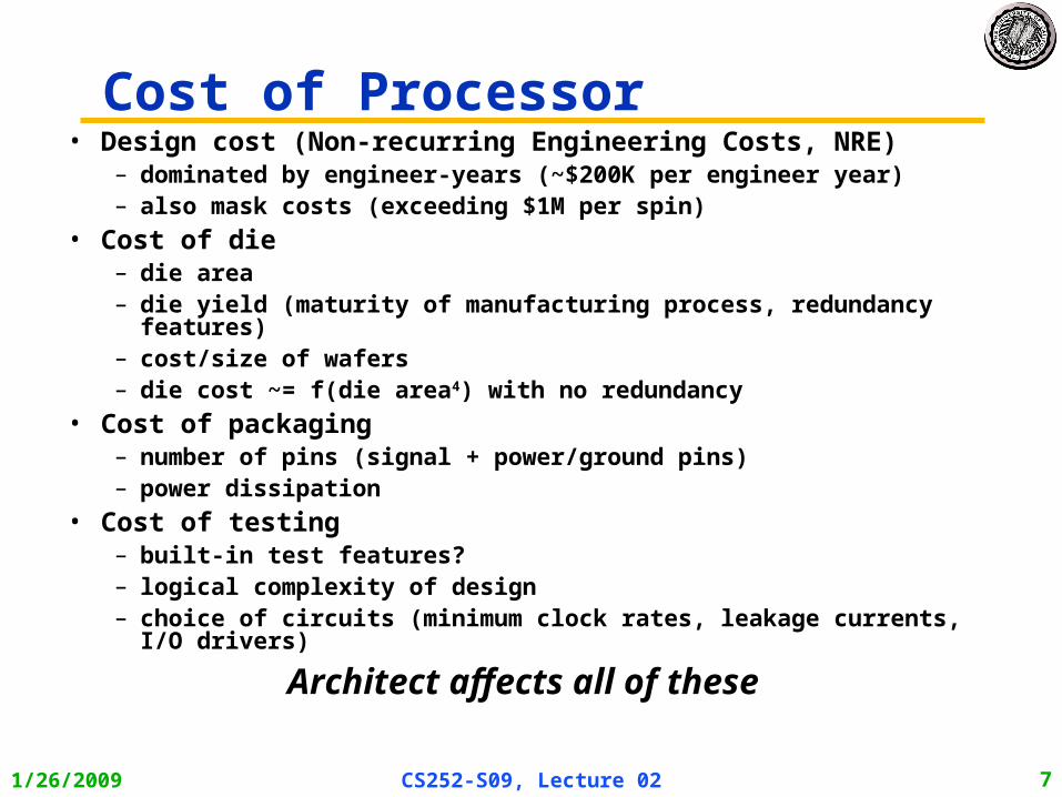
Cost of Processor• Design cost (Non-recurring Engineering Costs, NRE)
– dominated by engineer-years (~$200K per engineer year)– also mask costs (exceeding $1M per spin)
• Cost of die– die area– die yield (maturity of manufacturing process, redundancy features)– cost/size of wafers– die cost ~= f(die area4) with no redundancy
• Cost of packaging– number of pins (signal + power/ground pins)– power dissipation
• Cost of testing– built-in test features?– logical complexity of design– choice of circuits (minimum clock rates, leakage currents, I/O drivers)
Architect affects all of these

1/26/2009 CS252-S09, Lecture 02 8
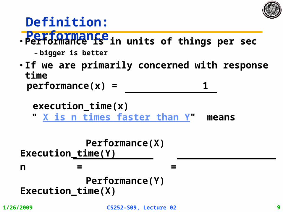
What is Performance?
• Latency (or response time or execution time)– time to complete one task
• Bandwidth (or throughput)– tasks completed per unit time
1/26/2009 CS252-S09, Lecture 02 9
Performance(X) Execution_time(Y)
n = =
Performance(Y) Execution_time(X)
Definition: Performance• Performance is in units of things per sec
– bigger is better
• If we are primarily concerned with response time
performance(x) = 1 execution_time(x)
" X is n times faster than Y" means

1/26/2009 CS252-S09, Lecture 02 10
Performance: What to measure
• Usually rely on benchmarks vs. real workloads
• To increase predictability, collections of benchmark applications-- benchmark suites -- are popular
• SPECCPU: popular desktop benchmark suite– CPU only, split between integer and floating point programs
– SPECint2000 has 12 integer, SPECfp2000 has 14 integer pgms
– SPECCPU2006 to be announced Spring 2006
– SPECSFS (NFS file server) and SPECWeb (WebServer) added as server benchmarks
• Transaction Processing Council measures server performance and cost-performance for databases
– TPC-C Complex query for Online Transaction Processing
– TPC-H models ad hoc decision support
– TPC-W a transactional web benchmark
– TPC-App application server and web services benchmark
1/26/2009 CS252-S09, Lecture 02 11
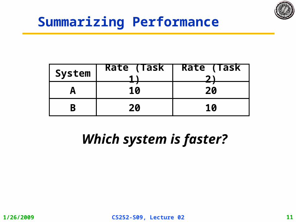
Summarizing Performance
Which system is faster?
System Rate (Task 1) Rate (Task 2)
A 10 20
B 20 10
1/26/2009 CS252-S09, Lecture 02 12
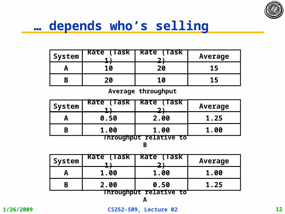
… depends who’s selling
System Rate (Task 1) Rate (Task 2)
A 10 20
B 20 10
Average
15
15
Average throughput
System Rate (Task 1) Rate (Task 2)
A 0.50 2.00
B 1.00 1.00
Average
1.25
1.00
Throughput relative to B
System Rate (Task 1) Rate (Task 2)
A 1.00 1.00
B 2.00 0.50
Average
1.00
1.25
Throughput relative to A
1/26/2009 CS252-S09, Lecture 02 13
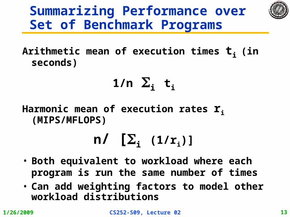
Summarizing Performance over Set of Benchmark Programs
Arithmetic mean of execution times ti (in seconds)
1/n i ti
Harmonic mean of execution rates ri (MIPS/MFLOPS)
n/ [i (1/ri)]
• Both equivalent to workload where each program is run the same number of times
• Can add weighting factors to model other workload distributions
1/26/2009 CS252-S09, Lecture 02 14
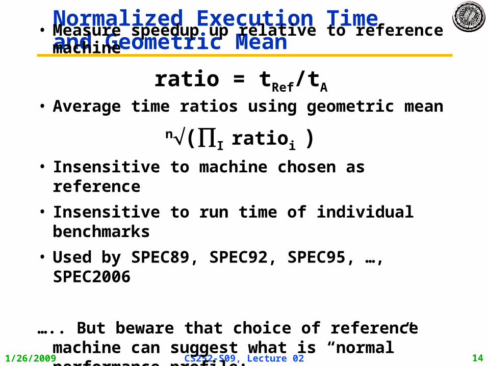
Normalized Execution Timeand Geometric Mean
• Measure speedup up relative to reference machine
ratio = tRef/tA
• Average time ratios using geometric mean
n(I ratioi )• Insensitive to machine chosen as reference
• Insensitive to run time of individual benchmarks
• Used by SPEC89, SPEC92, SPEC95, …, SPEC2006
….. But beware that choice of reference machine can suggest what is “normal” performance profile:
1/26/2009 CS252-S09, Lecture 02 15
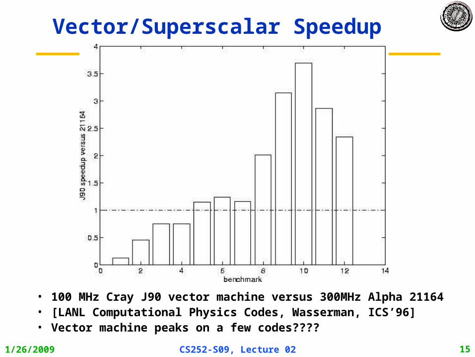
Vector/Superscalar Speedup
• 100 MHz Cray J90 vector machine versus 300MHz Alpha 21164• [LANL Computational Physics Codes, Wasserman, ICS’96]• Vector machine peaks on a few codes????
1/26/2009 CS252-S09, Lecture 02 16
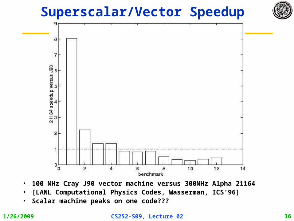
Superscalar/Vector Speedup
• 100 MHz Cray J90 vector machine versus 300MHz Alpha 21164• [LANL Computational Physics Codes, Wasserman, ICS’96]• Scalar machine peaks on one code???
1/26/2009 CS252-S09, Lecture 02 17
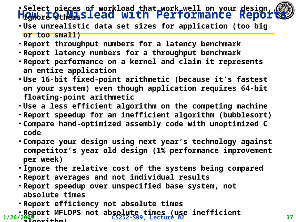
How to Mislead with Performance Reports
• Select pieces of workload that work well on your design, ignore others• Use unrealistic data set sizes for application (too big or too small)• Report throughput numbers for a latency benchmark• Report latency numbers for a throughput benchmark• Report performance on a kernel and claim it represents an entire
application• Use 16-bit fixed-point arithmetic (because it’s fastest on your system)
even though application requires 64-bit floating-point arithmetic• Use a less efficient algorithm on the competing machine• Report speedup for an inefficient algorithm (bubblesort)• Compare hand-optimized assembly code with unoptimized C code• Compare your design using next year’s technology against
competitor’s year old design (1% performance improvement per week)• Ignore the relative cost of the systems being compared• Report averages and not individual results• Report speedup over unspecified base system, not absolute times• Report efficiency not absolute times• Report MFLOPS not absolute times (use inefficient algorithm)[ David Bailey “Twelve ways to fool the masses when giving performance
results for parallel supercomputers” ]
1/26/2009 CS252-S09, Lecture 02 18
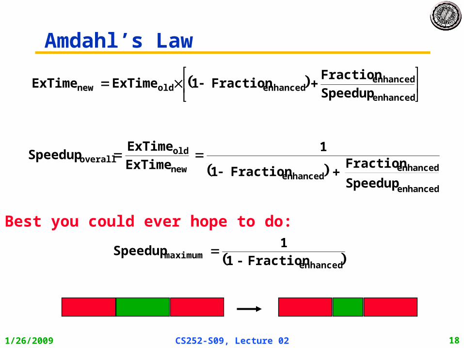
Amdahl’s Law
enhanced
enhancedenhanced
new
oldoverall
Speedup
Fraction Fraction
1
ExTimeExTime
Speedup
1
Best you could ever hope to do:
enhancedmaximum Fraction - 1
1 Speedup
enhanced
enhancedenhancedoldnew Speedup
FractionFraction ExTime ExTime 1

1/26/2009 CS252-S09, Lecture 02 19
Amdahl’s Law example
• New CPU 10X faster
• I/O bound server, so 60% time waiting for I/O
• Apparently, its human nature to be attracted by 10X faster, vs. keeping in perspective its just 1.6X faster
56.1
64.0
1
100.4
0.4 1
1
SpeedupFraction
Fraction 1
1 Speedup
enhanced
enhancedenhanced
overall
1/26/2009 CS252-S09, Lecture 02 20
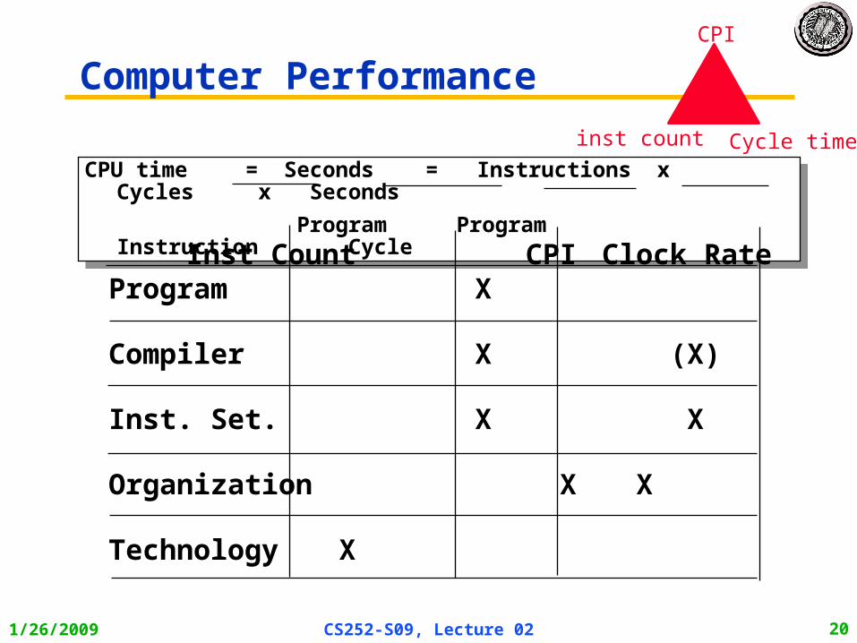
Computer Performance
CPU time = Seconds = Instructions x Cycles x Seconds
Program Program Instruction Cycle
CPU time = Seconds = Instructions x Cycles x Seconds
Program Program Instruction Cycle
Inst Count CPI Clock RateProgram X
Compiler X (X)
Inst. Set. X X
Organization X X
Technology X
inst count
CPI
Cycle time
1/26/2009 CS252-S09, Lecture 02 21
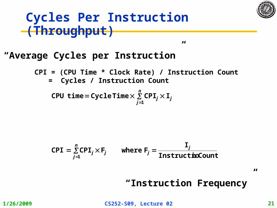
Cycles Per Instruction (Throughput)
“Instruction Frequency”
CPI = (CPU Time * Clock Rate) / Instruction Count = Cycles / Instruction Count
“Average Cycles per Instruction”
j
n
jj I CPI TimeCycle time CPU
1
Count nInstructio
I F where F CPI CPI j
j
n
jjj
1
1/26/2009 CS252-S09, Lecture 02 22
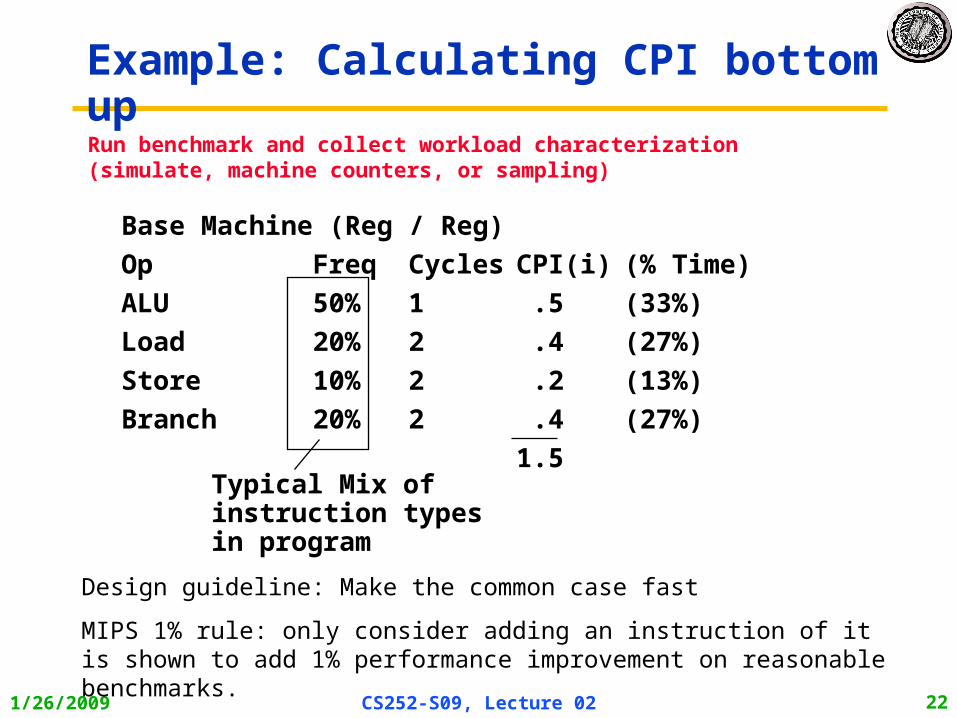
Example: Calculating CPI bottom up
Typical Mix of instruction typesin program
Base Machine (Reg / Reg)
Op Freq Cycles CPI(i) (% Time)
ALU 50% 1 .5 (33%)
Load 20% 2 .4 (27%)
Store 10% 2 .2 (13%)
Branch 20% 2 .4 (27%)
1.5
Design guideline: Make the common case fast
MIPS 1% rule: only consider adding an instruction of it is shown to add 1% performance improvement on reasonable benchmarks.
Run benchmark and collect workload characterization (simulate, machine counters, or sampling)
1/26/2009 CS252-S09, Lecture 02 23
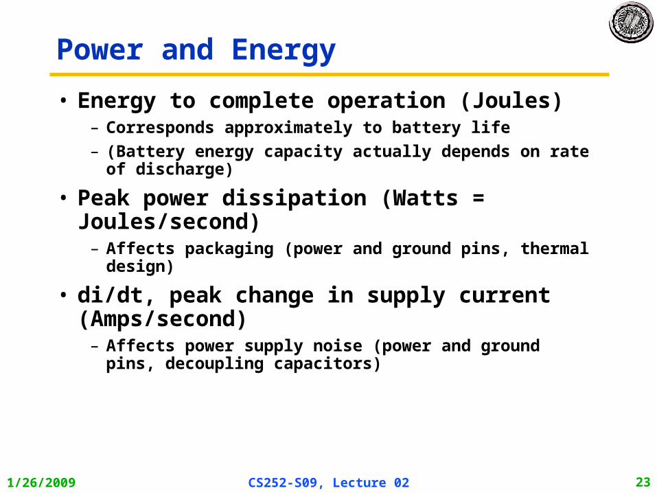
Power and Energy
• Energy to complete operation (Joules)– Corresponds approximately to battery life
– (Battery energy capacity actually depends on rate of discharge)
• Peak power dissipation (Watts = Joules/second)– Affects packaging (power and ground pins, thermal design)
• di/dt, peak change in supply current (Amps/second)
– Affects power supply noise (power and ground pins, decoupling capacitors)
1/26/2009 CS252-S09, Lecture 02 24
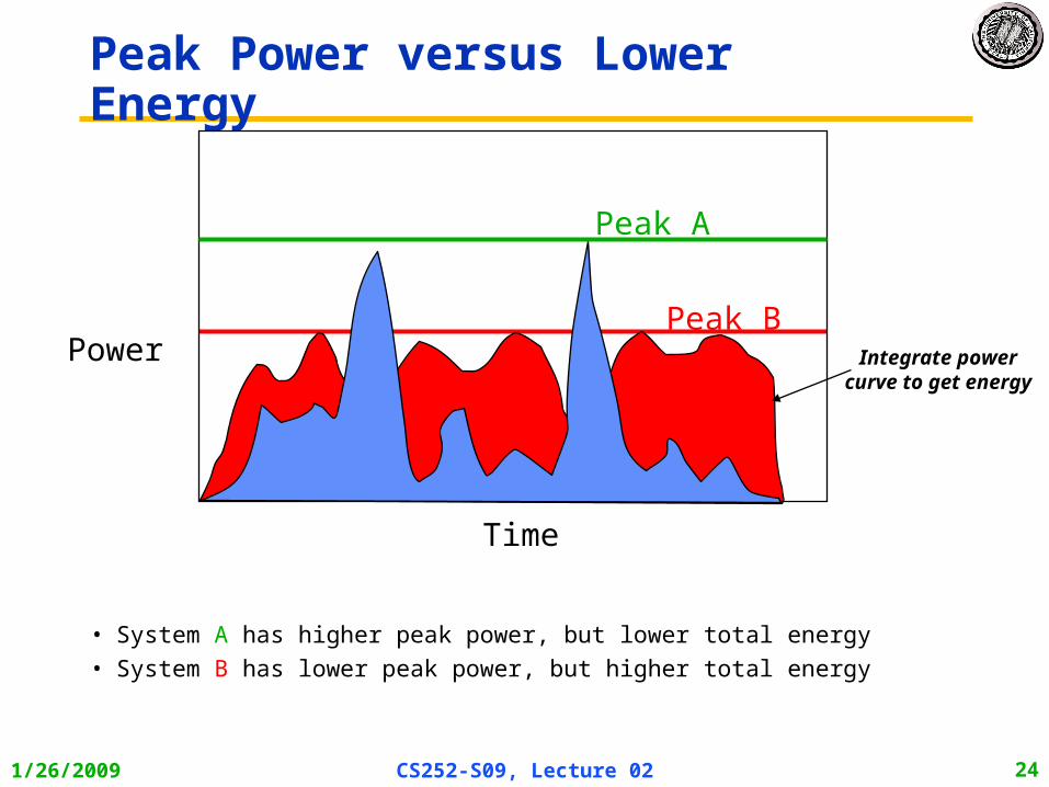
Peak Power versus Lower Energy
• System A has higher peak power, but lower total energy
• System B has lower peak power, but higher total energy
Power
Time
Peak A
Peak BIntegrate power
curve to get energy

1/26/2009 CS252-S09, Lecture 02 25
CS 252 Administrivia
• Sign up! Web site is (doesn’t quite work!): http://www.cs.berkeley.edu/~kubitron/cs252
• Review: Chapter 1, Appendix A, B, C• CS 152 home page, maybe “Computer Organization
and Design (COD)2/e” – If did take a class, be sure COD Chapters 2, 5, 6, 7 are familiar– Copies in Bechtel Library on 2-hour reserve
• First two readings are up (look on Lecture page)– Read the assignment carefully, since the requirements vary about
what you need to turn in– Submit results to website before class
» (will be a link up on handouts page)– You can have 5 total late days on assignments
» 10% per day afterwards» Save late days!
1/26/2009 CS252-S09, Lecture 02 26
CS 252 Administrivia
• Resources for course on web site:– Check out the ISCA (International Symposium on Computer
Architecture) 25th year retrospective on web site.Look for “Additional reading” below text-book description
– Pointers to previous CS152 exams and resources
– Lots of old CS252 material
– Interesting links. Check out the:WWW Computer Architecture Home Page
• Size of class seems ok:– I asked Michael David to put everyone on waitlist into class
– Check to make sure
1/26/2009 CS252-S09, Lecture 02 27
ISA Implementation Review
1/26/2009 CS252-S09, Lecture 02 28
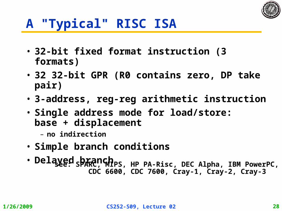
A "Typical" RISC ISA
• 32-bit fixed format instruction (3 formats)
• 32 32-bit GPR (R0 contains zero, DP take pair)
• 3-address, reg-reg arithmetic instruction
• Single address mode for load/store: base + displacement
– no indirection
• Simple branch conditions
• Delayed branch
see: SPARC, MIPS, HP PA-Risc, DEC Alpha, IBM PowerPC, CDC 6600, CDC 7600, Cray-1, Cray-2, Cray-3
1/26/2009 CS252-S09, Lecture 02 29
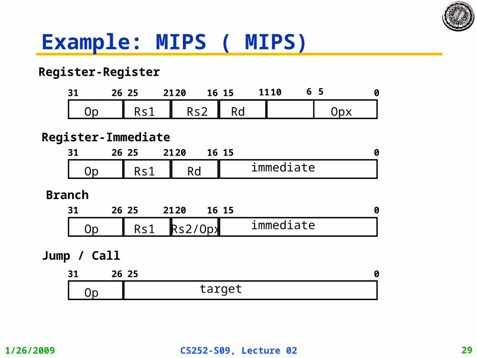
Example: MIPS ( MIPS)
Op
31 26 01516202125
Rs1 Rd immediate
Op
31 26 025
Op
31 26 01516202125
Rs1 Rs2
target
Rd Opx
Register-Register
561011
Register-Immediate
Op
31 26 01516202125
Rs1 Rs2/Opx immediate
Branch
Jump / Call
1/26/2009 CS252-S09, Lecture 02 30
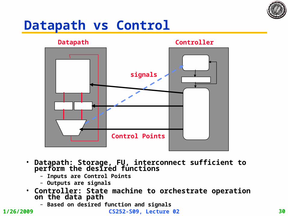
Datapath vs Control
• Datapath: Storage, FU, interconnect sufficient to perform the desired functions
– Inputs are Control Points– Outputs are signals
• Controller: State machine to orchestrate operation on the data path
– Based on desired function and signals
Datapath Controller
Control Points
signals

1/26/2009 CS252-S09, Lecture 02 31
Simple Pipelining Review

1/26/2009 CS252-S09, Lecture 02 32
5 Steps of MIPS DatapathMemoryAccess
Write
Back
InstructionFetch
Instr. DecodeReg. Fetch
ExecuteAddr. Calc
ALU
Mem
ory
Reg File
MU
XM
UX
Data
Mem
ory
MU
X
SignExtend
Zero?
IF/ID
ID/E
X
MEM
/WB
EX
/MEM
4
Ad
der
Next SEQ PC Next SEQ PC
RD RD RD WB
Data
• Data stationary control– local decode for each instruction phase / pipeline stage
Next PC
Addre
ss
RS1
RS2
Imm
MU
X
IR <= mem[PC]; PC <= PC + 4
A <= Reg[IRrs];
B <= Reg[IRrt]
rslt <= A opIRop B
Reg[IRrd] <= WB
WB <= rslt
1/26/2009 CS252-S09, Lecture 02 33
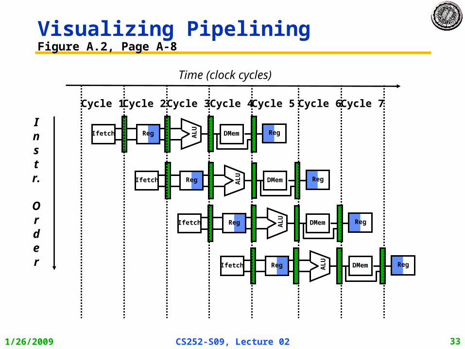
Visualizing PipeliningFigure A.2, Page A-8
Instr.
Order
Time (clock cycles)
Reg
ALU
DMemIfetch Reg
Reg
ALU
DMemIfetch Reg
Reg
ALU
DMemIfetch Reg
Reg
ALU
DMemIfetch Reg
Cycle 1Cycle 2 Cycle 3Cycle 4 Cycle 6Cycle 7Cycle 5
1/26/2009 CS252-S09, Lecture 02 34
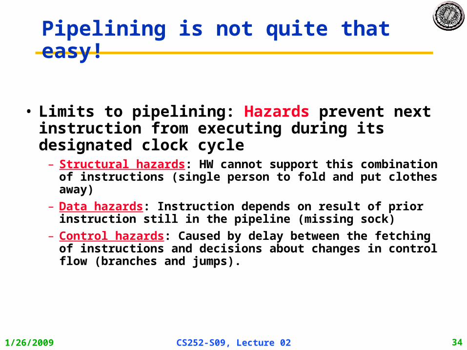
Pipelining is not quite that easy!
• Limits to pipelining: Hazards prevent next instruction from executing during its designated clock cycle
– Structural hazards: HW cannot support this combination of instructions (single person to fold and put clothes away)
– Data hazards: Instruction depends on result of prior instruction still in the pipeline (missing sock)
– Control hazards: Caused by delay between the fetching of instructions and decisions about changes in control flow (branches and jumps).
1/26/2009 CS252-S09, Lecture 02 35
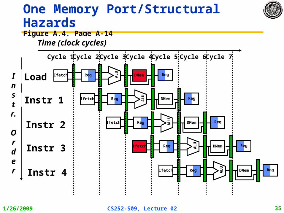
One Memory Port/Structural HazardsFigure A.4, Page A-14
Instr.
Order
Time (clock cycles)
Load
Instr 1
Instr 2
Instr 3
Instr 4
Reg
ALU
DMemIfetch Reg
Reg
ALU
DMemIfetch Reg
Reg
ALU
DMemIfetch Reg
Reg
ALU
DMemIfetch Reg
Cycle 1Cycle 2 Cycle 3Cycle 4 Cycle 6Cycle 7Cycle 5
Reg
ALU
DMemIfetch Reg
1/26/2009 CS252-S09, Lecture 02 36
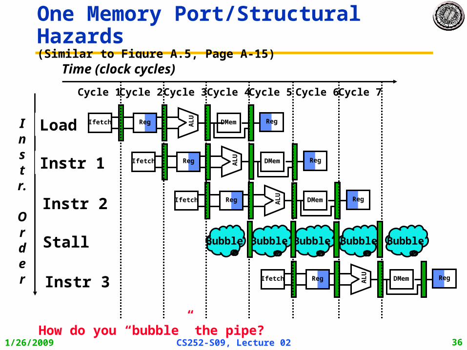
One Memory Port/Structural Hazards(Similar to Figure A.5, Page A-15)
Instr.
Order
Time (clock cycles)
Load
Instr 1
Instr 2
Stall
Instr 3
Reg
ALU
DMemIfetch Reg
Reg
ALU
DMemIfetch Reg
Reg
ALU
DMemIfetch Reg
Cycle 1Cycle 2 Cycle 3Cycle 4 Cycle 6Cycle 7Cycle 5
Reg
ALU
DMemIfetch Reg
Bubble Bubble Bubble BubbleBubble
How do you “bubble” the pipe?
1/26/2009 CS252-S09, Lecture 02 37
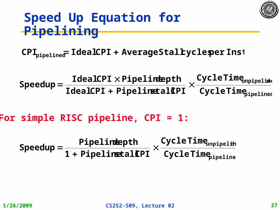
Speed Up Equation for Pipelining
pipelined
dunpipeline
TimeCycle
TimeCycle
CPI stall Pipeline CPI Idealdepth Pipeline CPI Ideal
Speedup
pipelined
dunpipeline
TimeCycle
TimeCycle
CPI stall Pipeline 1depth Pipeline
Speedup
Instper cycles Stall Average CPI Ideal CPIpipelined
For simple RISC pipeline, CPI = 1:
1/26/2009 CS252-S09, Lecture 02 38
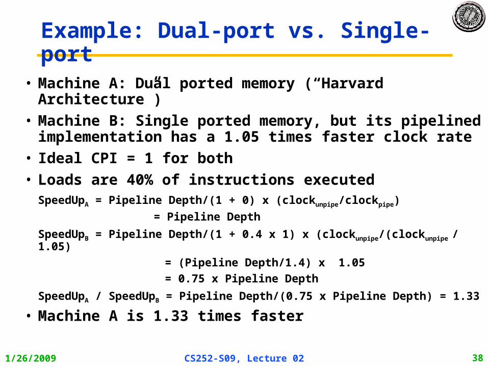
Example: Dual-port vs. Single-port
• Machine A: Dual ported memory (“Harvard Architecture”)
• Machine B: Single ported memory, but its pipelined implementation has a 1.05 times faster clock rate
• Ideal CPI = 1 for both
• Loads are 40% of instructions executedSpeedUpA = Pipeline Depth/(1 + 0) x (clockunpipe/clockpipe)
= Pipeline Depth
SpeedUpB = Pipeline Depth/(1 + 0.4 x 1) x (clockunpipe/(clockunpipe / 1.05)
= (Pipeline Depth/1.4) x 1.05
= 0.75 x Pipeline Depth
SpeedUpA / SpeedUpB = Pipeline Depth/(0.75 x Pipeline Depth) = 1.33
• Machine A is 1.33 times faster

1/26/2009 CS252-S09, Lecture 02 39
Instr.
Order
add r1,r2,r3
sub r4,r1,r3
and r6,r1,r7
or r8,r1,r9
xor r10,r1,r11
Reg
ALU
DMemIfetch Reg
Reg
ALU
DMemIfetch Reg
Reg
ALU
DMemIfetch Reg
Reg
ALU
DMemIfetch Reg
Reg
ALU
DMemIfetch Reg
Data Hazard on R1
Time (clock cycles)
IF ID/RF EX MEM WB
1/26/2009 CS252-S09, Lecture 02 40
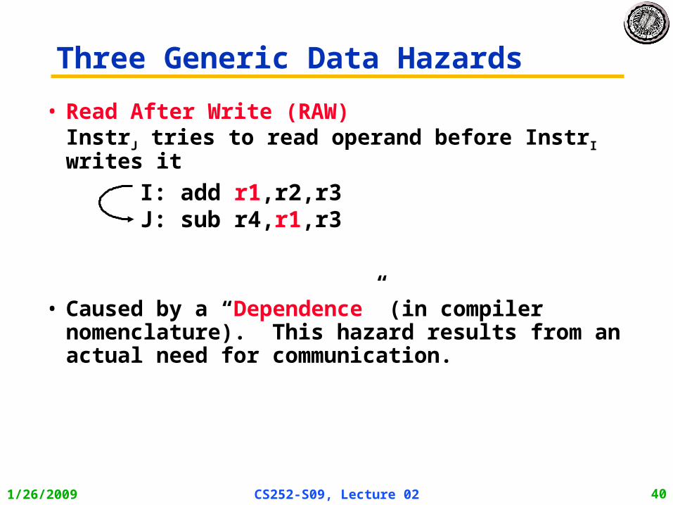
• Read After Write (RAW) InstrJ tries to read operand before InstrI writes it
• Caused by a “Dependence” (in compiler nomenclature). This hazard results from an actual need for communication.
Three Generic Data Hazards
I: add r1,r2,r3J: sub r4,r1,r3

1/26/2009 CS252-S09, Lecture 02 41
• Write After Read (WAR) InstrJ writes operand before InstrI reads it
• Called an “anti-dependence” by compiler writers.This results from reuse of the name “r1”.
• Can’t happen in MIPS 5 stage pipeline because:
– All instructions take 5 stages, and
– Reads are always in stage 2, and
– Writes are always in stage 5
I: sub r4,r1,r3 J: add r1,r2,r3K: mul r6,r1,r7
Three Generic Data Hazards

1/26/2009 CS252-S09, Lecture 02 42
Three Generic Data Hazards
• Write After Write (WAW) InstrJ writes operand before InstrI writes it.
• Called an “output dependence” by compiler writersThis also results from the reuse of name “r1”.
• Can’t happen in MIPS 5 stage pipeline because:
– All instructions take 5 stages, and
– Writes are always in stage 5
• Will see WAR and WAW in more complicated pipes
I: sub r1,r4,r3 J: add r1,r2,r3K: mul r6,r1,r7

1/26/2009 CS252-S09, Lecture 02 43
Time (clock cycles)
Forwarding to Avoid Data Hazard
Inst
r.
Order
add r1,r2,r3
sub r4,r1,r3
and r6,r1,r7
or r8,r1,r9
xor r10,r1,r11
Reg
ALU
DMemIfetch Reg
Reg
ALU
DMemIfetch Reg
Reg
ALU
DMemIfetch Reg
Reg
ALU
DMemIfetch Reg
Reg
ALU
DMemIfetch Reg
1/26/2009 CS252-S09, Lecture 02 44
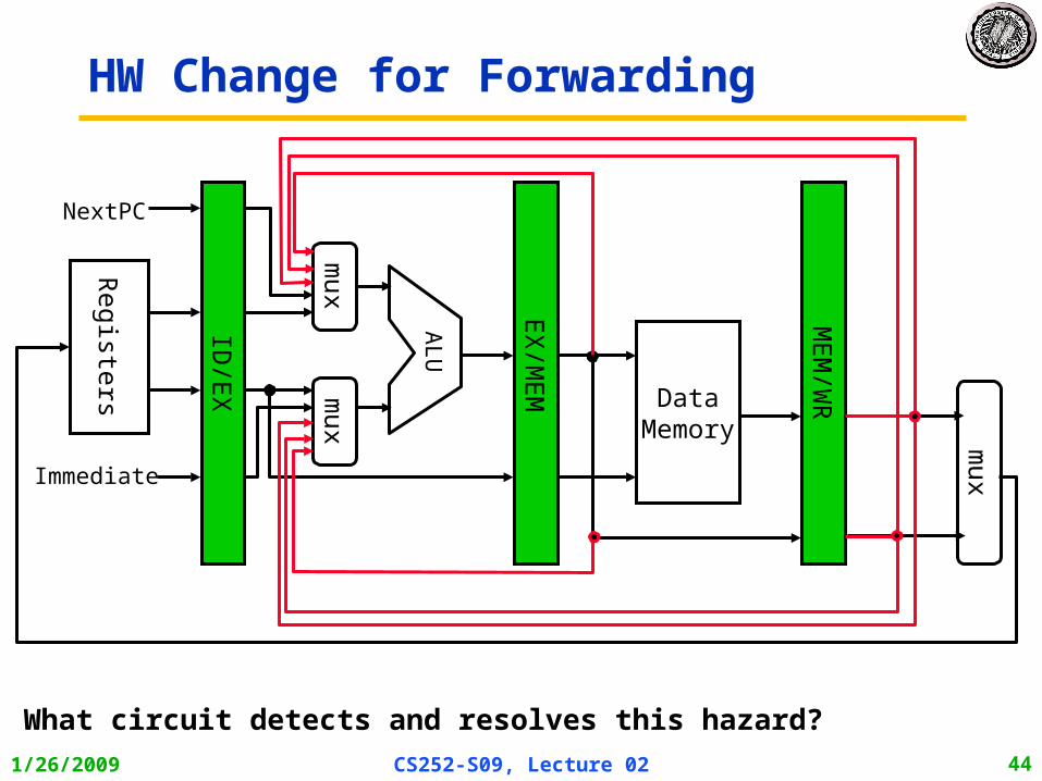
HW Change for Forwarding
MEM
/WR
ID/E
X
EX
/MEM
DataMemory
ALU
mux
mux
Registe
rs
NextPC
Immediate
mux
What circuit detects and resolves this hazard?
1/26/2009 CS252-S09, Lecture 02 45
Time (clock cycles)
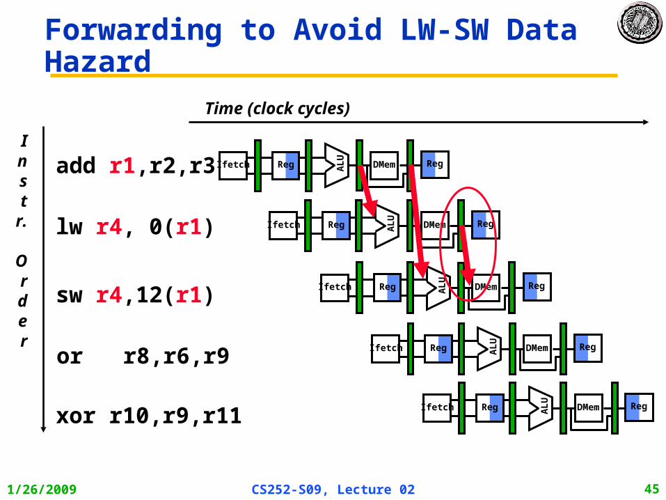
Forwarding to Avoid LW-SW Data Hazard
Inst
r.
Order
add r1,r2,r3
lw r4, 0(r1)
sw r4,12(r1)
or r8,r6,r9
xor r10,r9,r11
Reg
ALU
DMemIfetch Reg
Reg
ALU
DMemIfetch Reg
Reg
ALU
DMemIfetch Reg
Reg
ALU
DMemIfetch Reg
Reg
ALU
DMemIfetch Reg

1/26/2009 CS252-S09, Lecture 02 46
Time (clock cycles)
Instr.
Order
lw r1, 0(r2)
sub r4,r1,r6
and r6,r1,r7
or r8,r1,r9
Data Hazard Even with Forwarding
Reg
ALU
DMemIfetch Reg
Reg
ALU
DMemIfetch Reg
Reg ALU
DMemIfetch Reg
Reg
ALU
DMemIfetch Reg
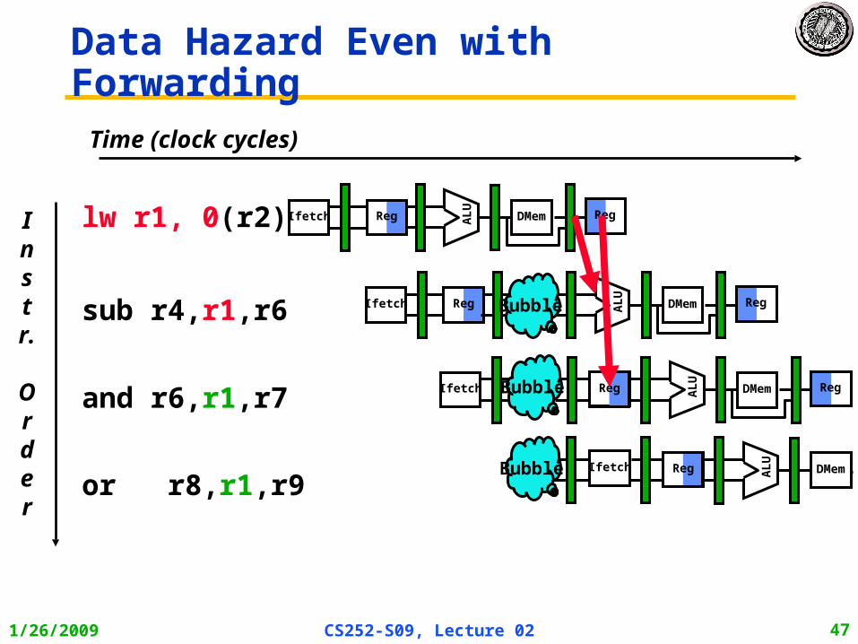
1/26/2009 CS252-S09, Lecture 02 47
Data Hazard Even with Forwarding
or r8,r1,r9
lw r1, 0(r2)
sub r4,r1,r6
and r6,r1,r7
Reg
ALU
DMemIfetch Reg
RegIfetch
ALU
DMem RegBubble
Ifetch
ALU
DMem RegBubble Reg
Ifetch
ALU
DMemBubble Reg
Time (clock cycles)
Instr.
Order
1/26/2009 CS252-S09, Lecture 02 48
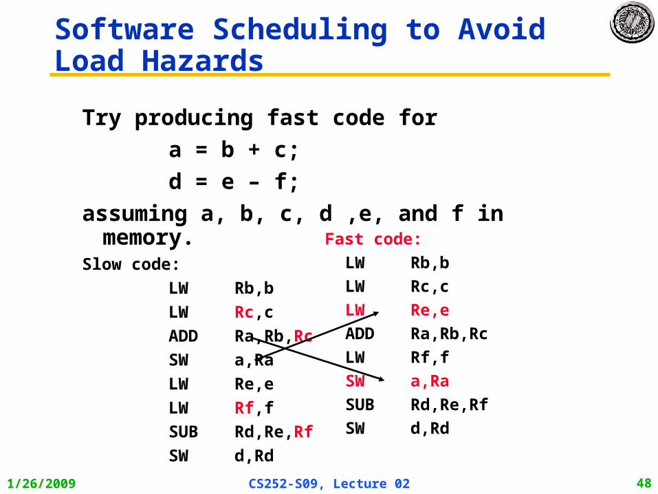
Try producing fast code for
a = b + c;
d = e – f;
assuming a, b, c, d ,e, and f in memory. Slow code:
LW Rb,b
LW Rc,c
ADD Ra,Rb,Rc
SW a,Ra
LW Re,e
LW Rf,f
SUB Rd,Re,Rf
SW d,Rd
Software Scheduling to Avoid Load Hazards
Fast code:
LW Rb,b
LW Rc,c
LW Re,e
ADD Ra,Rb,Rc
LW Rf,f
SW a,Ra
SUB Rd,Re,Rf
SW d,Rd

1/26/2009 CS252-S09, Lecture 02 49
Control Hazard on BranchesThree Stage Stall
10: beq r1,r3,36
14: and r2,r3,r5
18: or r6,r1,r7
22: add r8,r1,r9
36: xor r10,r1,r11
Reg ALU
DMemIfetch Reg
Reg
ALU
DMemIfetch Reg
Reg
ALU
DMemIfetch Reg
Reg
ALU
DMemIfetch Reg
Reg
ALU
DMemIfetch Reg
What do you do with the 3 instructions in between?
How do you do it?
Where is the “commit”?

1/26/2009 CS252-S09, Lecture 02 50
Branch Stall Impact
• If CPI = 1, 30% branch, Stall 3 cycles => new CPI = 1.9!
• Two part solution:– Determine branch taken or not sooner, AND
– Compute taken branch address earlier
• MIPS branch tests if register = 0 or 0
• MIPS Solution:– Move Zero test to ID/RF stage
– Adder to calculate new PC in ID/RF stage
– 1 clock cycle penalty for branch versus 3
1/26/2009 CS252-S09, Lecture 02 51
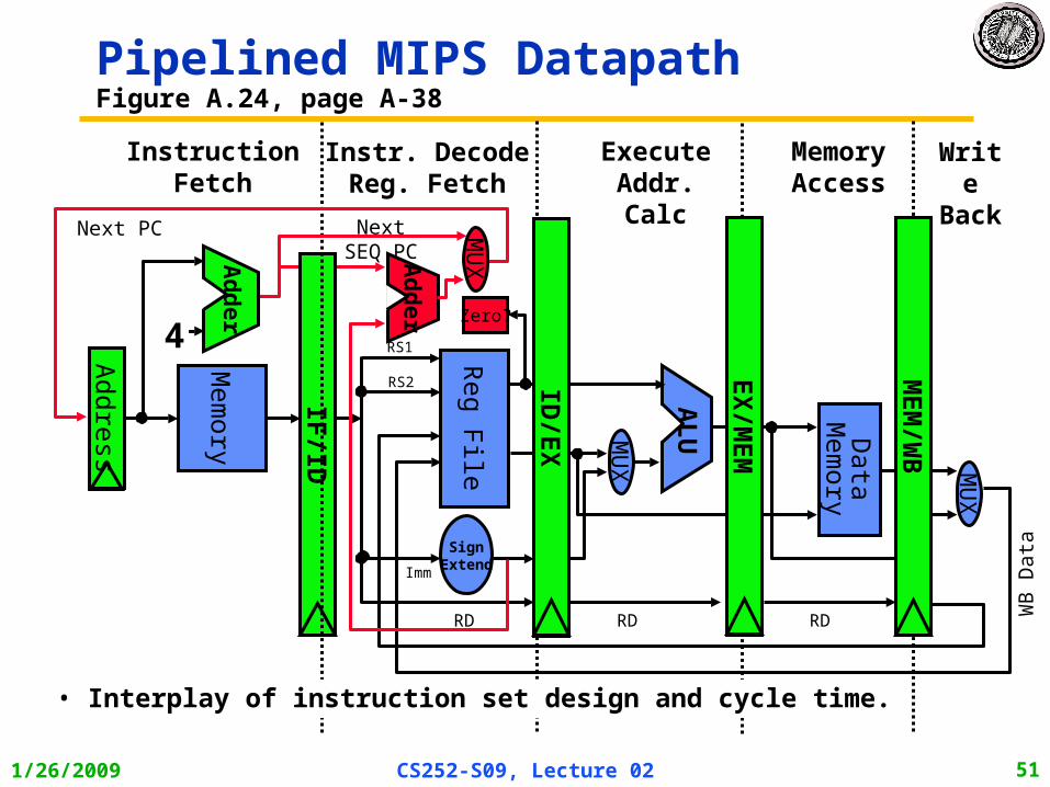
Ad
der
IF/ID
Pipelined MIPS DatapathFigure A.24, page A-38
MemoryAccess
Write
Back
InstructionFetch
Instr. DecodeReg. Fetch
ExecuteAddr. Calc
ALU
Mem
ory
Reg File
MU
X
Data
Mem
ory
MU
X
SignExtend
Zero?
MEM
/WB
EX
/MEM
4
Ad
der
Next SEQ PC
RD RD RD WB
Data
• Interplay of instruction set design and cycle time.
Next PC
Addre
ss
RS1
RS2
ImmM
UX
ID/E
X
1/26/2009 CS252-S09, Lecture 02 52
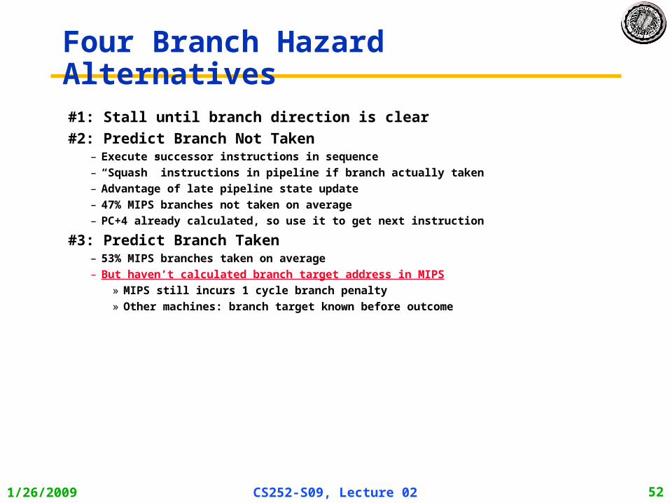
Four Branch Hazard Alternatives
#1: Stall until branch direction is clear
#2: Predict Branch Not Taken– Execute successor instructions in sequence
– “Squash” instructions in pipeline if branch actually taken
– Advantage of late pipeline state update
– 47% MIPS branches not taken on average
– PC+4 already calculated, so use it to get next instruction
#3: Predict Branch Taken– 53% MIPS branches taken on average
– But haven’t calculated branch target address in MIPS
» MIPS still incurs 1 cycle branch penalty
» Other machines: branch target known before outcome

1/26/2009 CS252-S09, Lecture 02 53
Four Branch Hazard Alternatives
#4: Delayed Branch– Define branch to take place AFTER a following instruction
branch instructionsequential successor1
sequential successor2
........sequential successorn
branch target if taken
– 1 slot delay allows proper decision and branch target address in 5 stage pipeline
– MIPS uses this
Branch delay of length n

1/26/2009 CS252-S09, Lecture 02 54
Scheduling Branch Delay Slots
• A is the best choice, fills delay slot & reduces instruction count (IC)
• In B, the sub instruction may need to be copied, increasing IC
• In B and C, must be okay to execute sub when branch fails
add $1,$2,$3if $2=0 then
delay slot
A. From before branch B. From branch target C. From fall through
add $1,$2,$3if $1=0 thendelay slot
add $1,$2,$3if $1=0 then
delay slot
sub $4,$5,$6
sub $4,$5,$6
becomes becomes becomes if $2=0 then
add $1,$2,$3add $1,$2,$3if $1=0 thensub $4,$5,$6
add $1,$2,$3if $1=0 then
sub $4,$5,$6

1/26/2009 CS252-S09, Lecture 02 55
Delayed Branch
• Compiler effectiveness for single branch delay slot:– Fills about 60% of branch delay slots
– About 80% of instructions executed in branch delay slots useful in computation
– About 50% (60% x 80%) of slots usefully filled
• Delayed Branch downside: As processor go to deeper pipelines and multiple issue, the branch delay grows and need more than one delay slot
– Delayed branching has lost popularity compared to more expensive but more flexible dynamic approaches
– Growth in available transistors has made dynamic approaches relatively cheaper
1/26/2009 CS252-S09, Lecture 02 56
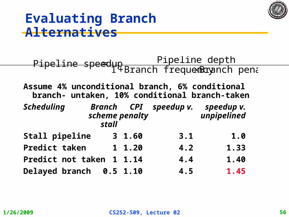
Evaluating Branch Alternatives
Assume 4% unconditional branch, 6% conditional branch- untaken, 10% conditional branch-taken
Scheduling Branch CPI speedup v. speedup v. scheme penalty unpipelined
stall
Stall pipeline 3 1.60 3.1 1.0
Predict taken 1 1.20 4.2 1.33
Predict not taken 1 1.14 4.4 1.40
Delayed branch 0.5 1.10 4.5 1.45
Pipeline speedup = Pipeline depth1 +Branch frequencyBranch penalty
1/26/2009 CS252-S09, Lecture 02 57
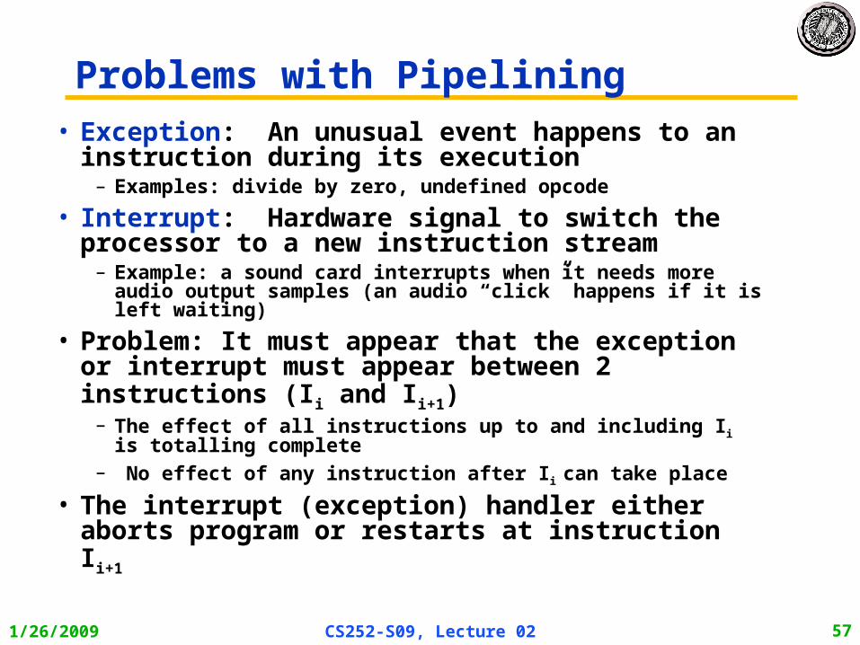
Problems with Pipelining• Exception: An unusual event happens to an
instruction during its execution – Examples: divide by zero, undefined opcode
• Interrupt: Hardware signal to switch the processor to a new instruction stream
– Example: a sound card interrupts when it needs more audio output samples (an audio “click” happens if it is left waiting)
• Problem: It must appear that the exception or interrupt must appear between 2 instructions (Ii and Ii+1)
– The effect of all instructions up to and including Ii is totalling complete
– No effect of any instruction after Ii can take place
• The interrupt (exception) handler either aborts program or restarts at instruction Ii+1

1/26/2009 CS252-S09, Lecture 02 58
Precise Exceptions in Static Pipelines
Key observation: architected state only change in memory and register write stages.

1/26/2009 CS252-S09, Lecture 02 59
Memory Hierarchy Review
1/26/2009 CS252-S09, Lecture 02 60
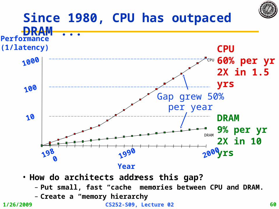
Since 1980, CPU has outpaced DRAM ...
CPU60% per yr2X in 1.5 yrs
DRAM9% per yr2X in 10 yrs
10
DRAM
CPU
Performance(1/latency)
100
1000
1980 20001990
Year
Gap grew 50% per year
• How do architects address this gap?– Put small, fast “cache” memories between CPU and DRAM.– Create a “memory hierarchy”

1/26/2009 CS252-S09, Lecture 02 61
1977: DRAM faster than microprocessors Apple ][ (1977)
Steve WozniakSteve
Jobs
CPU: 1000 ns DRAM: 400 ns
1/26/2009 CS252-S09, Lecture 02 62
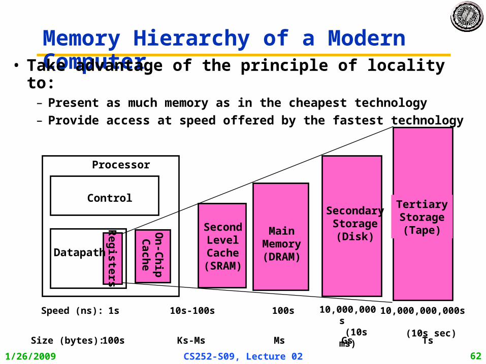
Memory Hierarchy of a Modern Computer• Take advantage of the principle of locality to:
– Present as much memory as in the cheapest technology
– Provide access at speed offered by the fastest technology
On
-Ch
ipC
ache
Registers
Control
Datapath
SecondaryStorage(Disk)
Processor
MainMemory(DRAM)
SecondLevelCache
(SRAM)
1s 10,000,000s
(10s ms)
Speed (ns): 10s-100s 100s
100s GsSize (bytes): Ks-Ms Ms
TertiaryStorage(Tape)
10,000,000,000s
(10s sec)Ts
1/26/2009 CS252-S09, Lecture 02 63
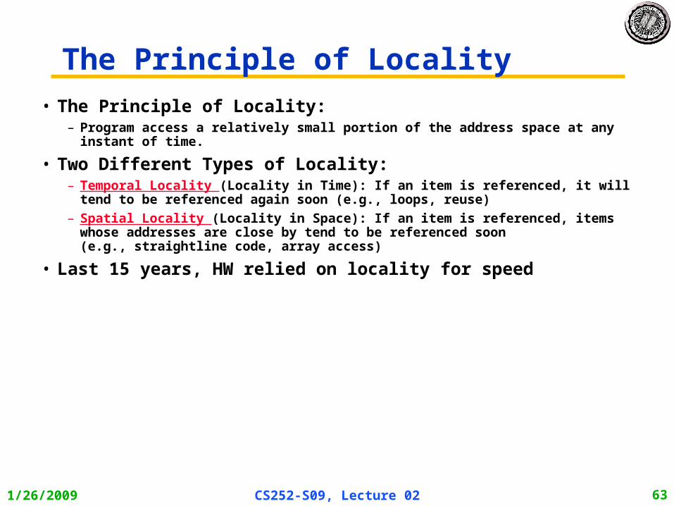
The Principle of Locality
• The Principle of Locality:– Program access a relatively small portion of the address space at any instant of time.
• Two Different Types of Locality:– Temporal Locality (Locality in Time): If an item is referenced, it will tend to be
referenced again soon (e.g., loops, reuse)
– Spatial Locality (Locality in Space): If an item is referenced, items whose addresses are close by tend to be referenced soon (e.g., straightline code, array access)
• Last 15 years, HW relied on locality for speed

1/26/2009 CS252-S09, Lecture 02 64
Programs with locality cache well ...
Donald J. Hatfield, Jeanette Gerald: Program Restructuring for Virtual Memory. IBM Systems Journal 10(3): 168-192 (1971)
Time
Mem
ory
Ad
dre
ss (
on
e d
ot
per
acc
ess)
SpatialLocality
Temporal Locality
Bad locality behavior

1/26/2009 CS252-S09, Lecture 02 65
Memory Hierarchy: Apple iMac G5
iMac G51.6 GHz
07 Reg L1 Inst L1 Data L2 DRAM Disk
Size 1K 64K 32K 512K 256M 80G
Latency
Cycles, Time
1,
0.6 ns
3,
1.9 ns
3,
1.9 ns
11,
6.9 ns
88,
55 ns
107,
12 ms
Let programs address a memory space that scales to the disk size, at
a speed that is usually as fast as register access
Managed by compiler
Managed by hardware
Managed by OS,hardware,
application
Goal: Illusion of large, fast, cheap memory
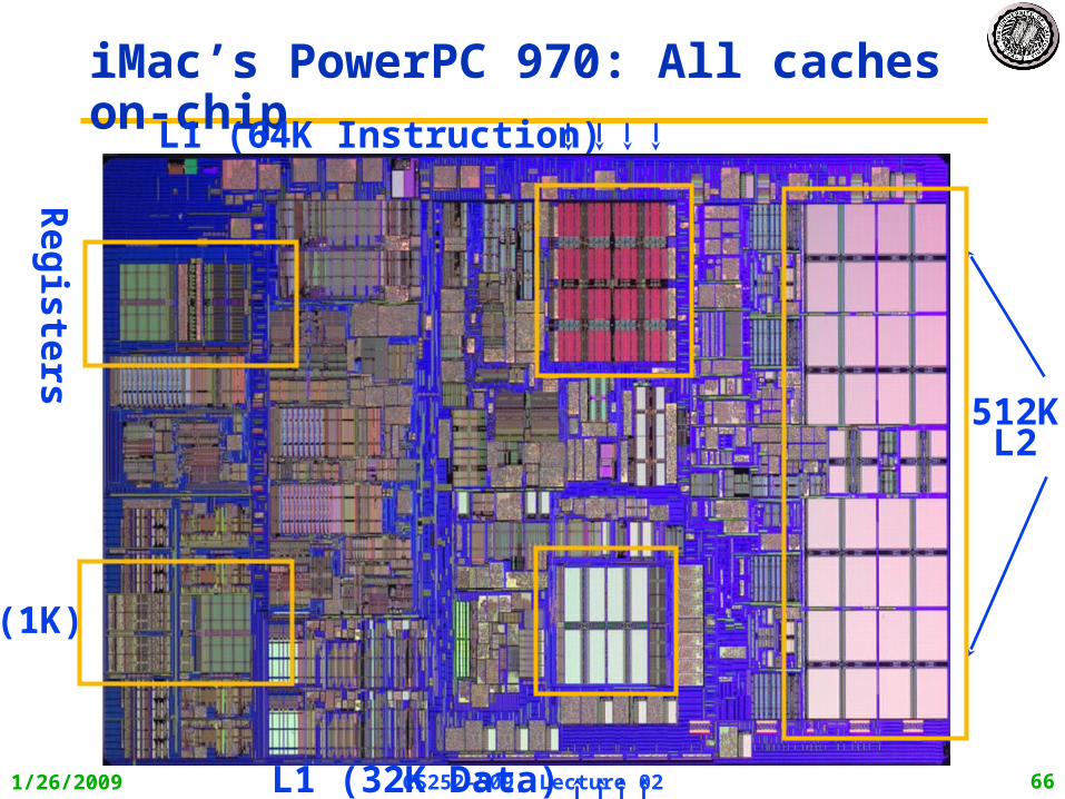
1/26/2009 CS252-S09, Lecture 02 66
iMac’s PowerPC 970: All caches on-chip
(1K)
Reg
isters
512KL2
L1 (64K Instruction)
L1 (32K Data)

1/26/2009 CS252-S09, Lecture 02 67
Memory Hierarchy: Terminology• Hit: data appears in some block in the upper level (example:
Block X) – Hit Rate: the fraction of memory access found in the upper level
– Hit Time: Time to access the upper level which consists of
RAM access time + Time to determine hit/miss
• Miss: data needs to be retrieve from a block in the lower level (Block Y)
– Miss Rate = 1 - (Hit Rate)
– Miss Penalty: Time to replace a block in the upper level +
Time to deliver the block the processor
• Hit Time << Miss Penalty (500 instructions on 21264!)
Lower LevelMemoryUpper Level
MemoryTo Processor
From ProcessorBlk X
Blk Y
1/26/2009 CS252-S09, Lecture 02 68
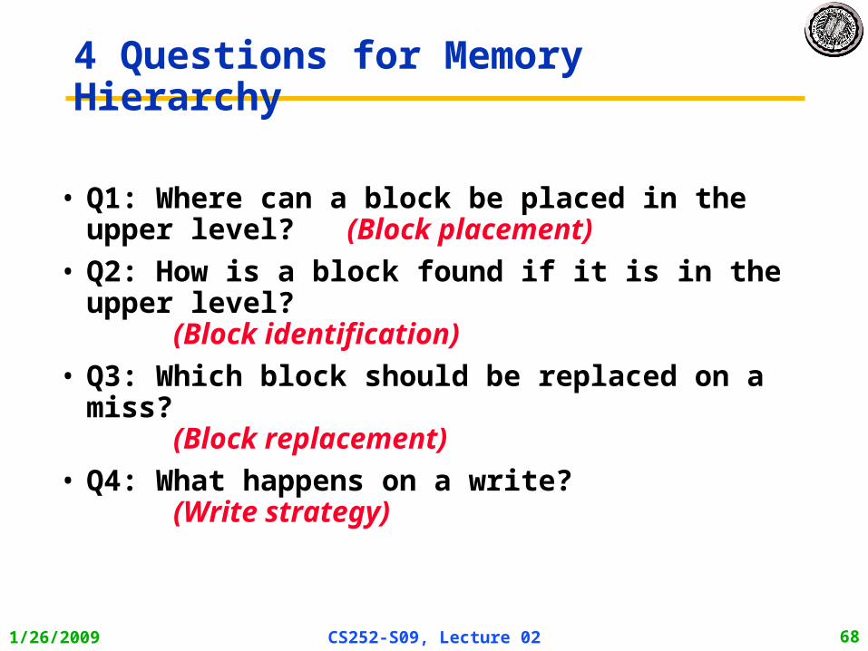
4 Questions for Memory Hierarchy
• Q1: Where can a block be placed in the upper level? (Block placement)
• Q2: How is a block found if it is in the upper level? (Block identification)
• Q3: Which block should be replaced on a miss? (Block replacement)
• Q4: What happens on a write? (Write strategy)
1/26/2009 CS252-S09, Lecture 02 69
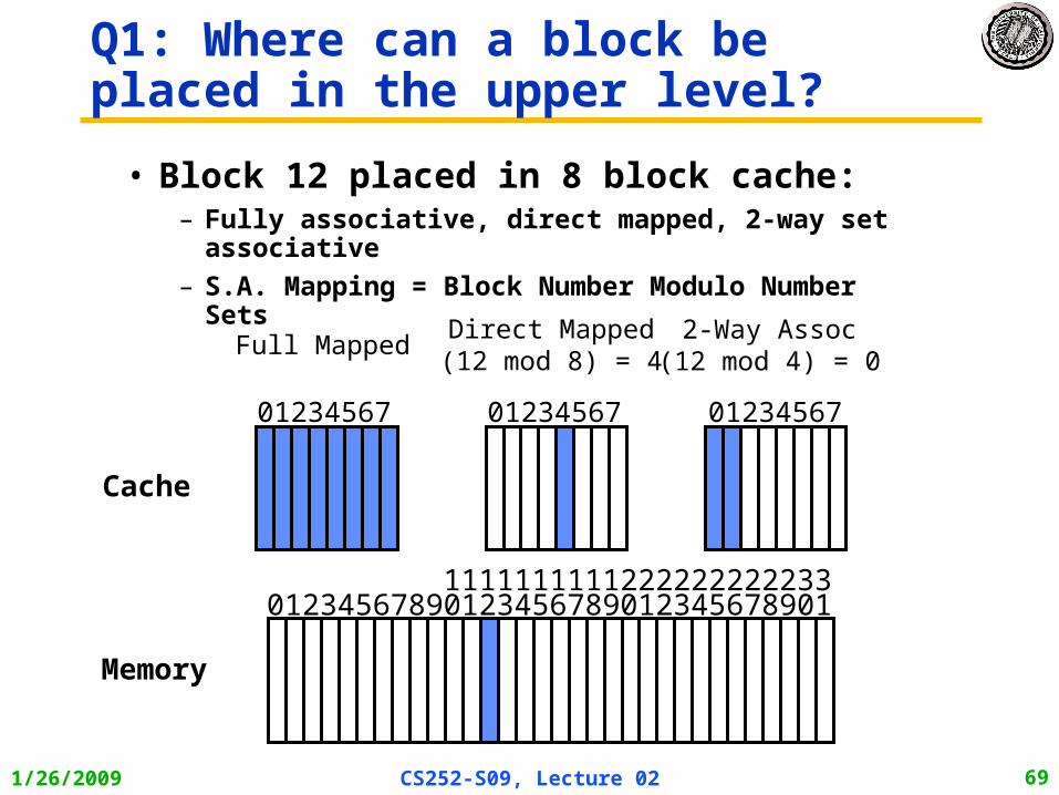
Q1: Where can a block be placed in the upper level?
• Block 12 placed in 8 block cache:– Fully associative, direct mapped, 2-way set associative
– S.A. Mapping = Block Number Modulo Number Sets
Cache
01234567 0123456701234567
Memory
111111111122222222223301234567890123456789012345678901
Full MappedDirect Mapped(12 mod 8) = 4
2-Way Assoc(12 mod 4) = 0
1/26/2009 CS252-S09, Lecture 02 70
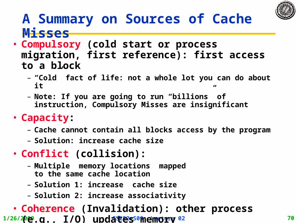
• Compulsory (cold start or process migration, first reference): first access to a block
– “Cold” fact of life: not a whole lot you can do about it
– Note: If you are going to run “billions” of instruction, Compulsory Misses are insignificant
• Capacity:– Cache cannot contain all blocks access by the program
– Solution: increase cache size
• Conflict (collision):– Multiple memory locations mapped
to the same cache location
– Solution 1: increase cache size
– Solution 2: increase associativity
• Coherence (Invalidation): other process (e.g., I/O) updates memory
A Summary on Sources of Cache Misses

1/26/2009 CS252-S09, Lecture 02 71
• Index Used to Lookup Candidates in Cache– Index identifies the set
• Tag used to identify actual copy– If no candidates match, then declare cache miss
• Block is minimum quantum of caching– Data select field used to select data within block
– Many caching applications don’t have data select field
Q2: How is a block found if it is in the upper level?
Blockoffset
Block AddressTag Index
Set Select
Data Select
1/26/2009 CS252-S09, Lecture 02 72
:
0x50
Valid Bit
:
Cache Tag
Byte 32
0
1
2
3
:
Cache Data
Byte 0Byte 1Byte 31 :
Byte 33Byte 63 :Byte 992Byte 1023 : 31
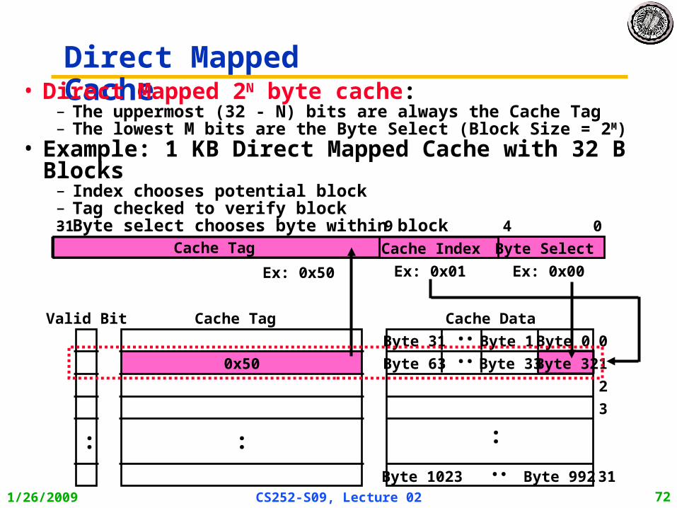
Direct Mapped Cache• Direct Mapped 2N byte cache:
– The uppermost (32 - N) bits are always the Cache Tag– The lowest M bits are the Byte Select (Block Size = 2M)
• Example: 1 KB Direct Mapped Cache with 32 B Blocks– Index chooses potential block– Tag checked to verify block– Byte select chooses byte within block
Ex: 0x50 Ex: 0x00
Cache Index
0431
Cache Tag Byte Select
9
Ex: 0x01

1/26/2009 CS252-S09, Lecture 02 73
Cache Index
0431
Cache Tag Byte Select
8
Cache Data
Cache Block 0
Cache TagValid
:: :
Cache Data
Cache Block 0
Cache Tag Valid
: ::
Mux 01Sel1 Sel0
OR
Hit
Set Associative Cache• N-way set associative: N entries per Cache Index
– N direct mapped caches operates in parallel• Example: Two-way set associative cache
– Cache Index selects a “set” from the cache– Two tags in the set are compared to input in parallel– Data is selected based on the tag result
Compare Compare
Cache Block
1/26/2009 CS252-S09, Lecture 02 74
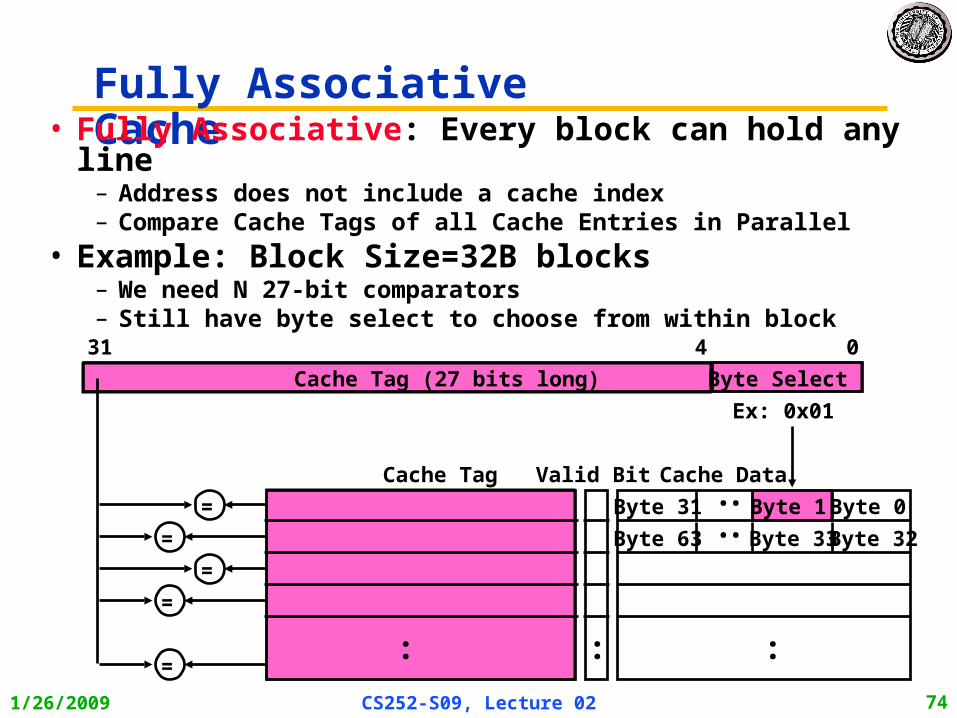
Fully Associative Cache• Fully Associative: Every block can hold any line– Address does not include a cache index– Compare Cache Tags of all Cache Entries in Parallel
• Example: Block Size=32B blocks– We need N 27-bit comparators– Still have byte select to choose from within block
:
Cache Data
Byte 0Byte 1Byte 31 :
Byte 32Byte 33Byte 63 :
Valid Bit
::
Cache Tag
04
Cache Tag (27 bits long) Byte Select
31
=
=
=
=
=
Ex: 0x01

1/26/2009 CS252-S09, Lecture 02 75
Q3: Which block should be replaced on a miss?
• Easy for Direct Mapped
• Set Associative or Fully Associative:– LRU (Least Recently Used): Appealing, but hard to
implement for high associativity
– Random: Easy, but – how well does it work?
Assoc: 2-way 4-way 8-way
Size LRU Ran LRU Ran LRU Ran
16K 5.2% 5.7% 4.7% 5.3% 4.4% 5.0%
64K 1.9% 2.0% 1.5% 1.7% 1.4% 1.5%
256K 1.15% 1.17% 1.13% 1.13% 1.12% 1.12%
1/26/2009 CS252-S09, Lecture 02 76
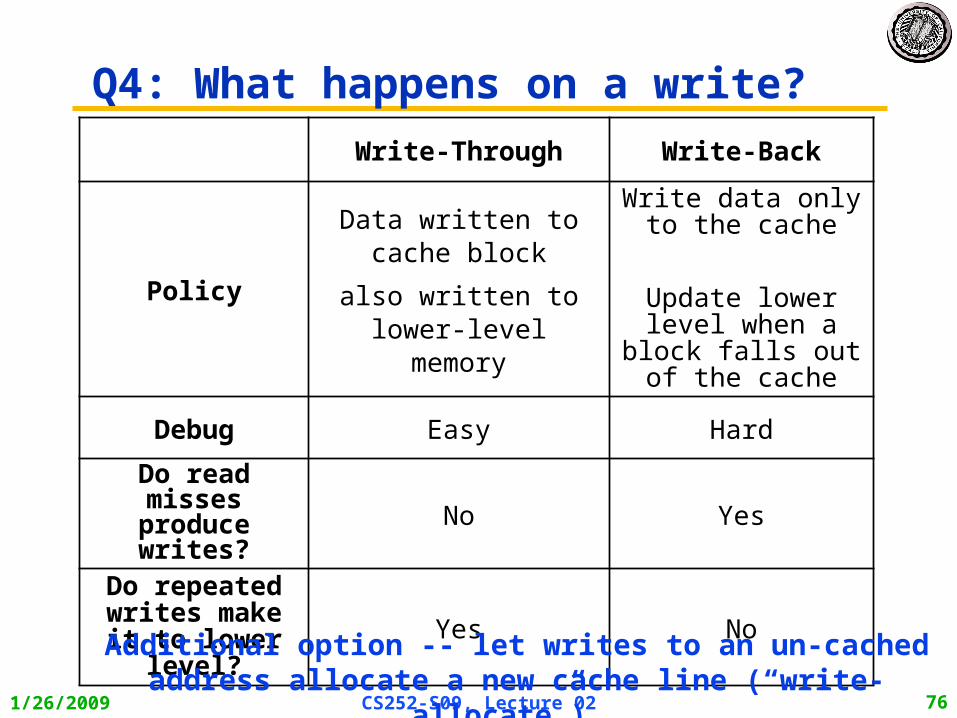
Q4: What happens on a write?
Write-Through Write-Back
Policy
Data written to cache block
also written to lower-level memory
Write data only to the cache
Update lower level when a block falls out of the cache
Debug Easy Hard
Do read misses produce writes? No Yes
Do repeated writes make it to
lower level?Yes No
Additional option -- let writes to an un-cached address allocate a new cache line (“write-
allocate”).

1/26/2009 CS252-S09, Lecture 02 77
Write Buffers for Write-Through Caches
Q. Why a write buffer ?
ProcessorCache
Write Buffer
Lower Level
Memory
Holds data awaiting write-through to lower level memory
A. So CPU doesn’t stall
Q. Why a buffer, why not just one register ?
A. Bursts of writes arecommon.Q. Are Read After
Write (RAW) hazards an issue for write buffer?
A. Yes! Drain buffer before next read, or check write buffers for match on reads
1/26/2009 CS252-S09, Lecture 02 78
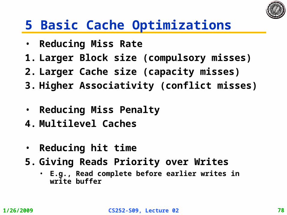
5 Basic Cache Optimizations• Reducing Miss Rate
1. Larger Block size (compulsory misses)
2. Larger Cache size (capacity misses)
3. Higher Associativity (conflict misses)
• Reducing Miss Penalty
4. Multilevel Caches
• Reducing hit time
5. Giving Reads Priority over Writes • E.g., Read complete before earlier writes in write buffer

1/26/2009 CS252-S09, Lecture 02 79
Virtual Memory
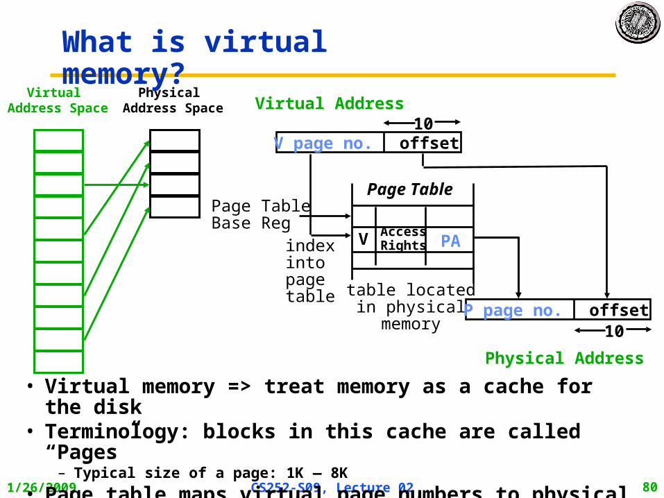
1/26/2009 CS252-S09, Lecture 02 80
• Virtual memory => treat memory as a cache for the disk• Terminology: blocks in this cache are called “Pages”
– Typical size of a page: 1K — 8K
• Page table maps virtual page numbers to physical frames– “PTE” = Page Table Entry
Physical Address Space
Virtual Address Space
What is virtual memory?
Virtual Address
Page Table
indexintopagetable
Page TableBase Reg
V AccessRights PA
V page no. offset10
table locatedin physicalmemory
P page no. offset10
Physical Address

1/26/2009 CS252-S09, Lecture 02 81
Three Advantages of Virtual Memory• Translation:
– Program can be given consistent view of memory, even though physical memory is scrambled
– Makes multithreading reasonable (now used a lot!)– Only the most important part of program (“Working Set”) must be in
physical memory.– Contiguous structures (like stacks) use only as much physical memory
as necessary yet still grow later.
• Protection:– Different threads (or processes) protected from each other.– Different pages can be given special behavior
» (Read Only, Invisible to user programs, etc).– Kernel data protected from User programs– Very important for protection from malicious programs
• Sharing:– Can map same physical page to multiple users
(“Shared memory”)

1/26/2009 CS252-S09, Lecture 02 82
PhysicalAddress: OffsetPhysical
Page #
4KB
Large Address Space Support10 bits 10 bits 12 bits
Virtual Address:
OffsetVirtualP2 index
VirtualP1 index
4 bytes
PageTablePtr
• Single-Level Page Table Large– 4KB pages for a 32-bit address 1M entries– Each process needs own page table!
• Multi-Level Page Table– Can allow sparseness of page table– Portions of table can be swapped to disk
4 bytes
1/26/2009 CS252-S09, Lecture 02 83
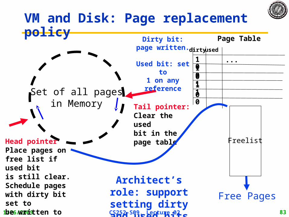
VM and Disk: Page replacement policy
...
Page Table
1 0
useddirty
1 00 11 10 0Set of all pages
in Memory Tail pointer:Clear the usedbit in thepage table
Head pointerPlace pages on free list if used bitis still clear.Schedule pages with dirty bit set tobe written to disk.
Freelist
Free Pages
Dirty bit: page written.
Used bit: set to
1 on any reference
Architect’s role: support setting dirty and used
bits
1/26/2009 CS252-S09, Lecture 02 84
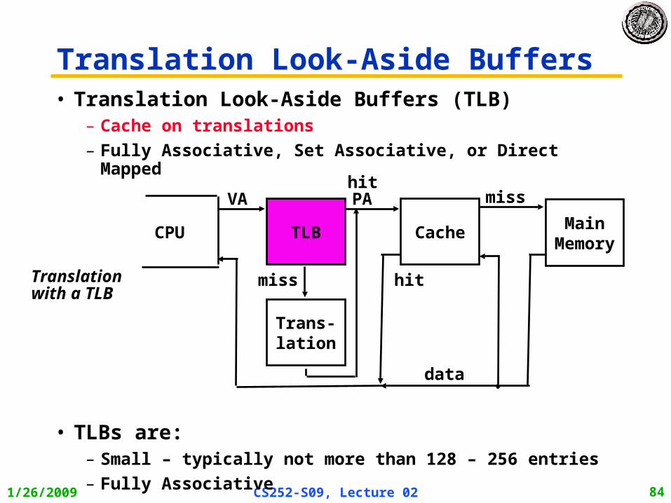
• Translation Look-Aside Buffers (TLB)– Cache on translations
– Fully Associative, Set Associative, or Direct Mapped
• TLBs are:– Small – typically not more than 128 – 256 entries
– Fully Associative
Translation Look-Aside Buffers
CPU TLB Cache MainMemory
VA PA miss
hit
data
Trans-lation
hit
missTranslationwith a TLB

1/26/2009 CS252-S09, Lecture 02 85
What Actually Happens on a TLB Miss?• Hardware traversed page tables:
– On TLB miss, hardware in MMU looks at current page table to fill TLB (may walk multiple levels)
» If PTE valid, hardware fills TLB and processor never knows» If PTE marked as invalid, causes Page Fault, after which kernel
decides what to do afterwards
• Software traversed Page tables (like MIPS)– On TLB miss, processor receives TLB fault– Kernel traverses page table to find PTE
» If PTE valid, fills TLB and returns from fault» If PTE marked as invalid, internally calls Page Fault handler
• Most chip sets provide hardware traversal– Modern operating systems tend to have more TLB faults since they use
translation for many things– Examples:
» shared segments» user-level portions of an operating system

1/26/2009 CS252-S09, Lecture 02 86
Example: R3000 pipeline
Inst Fetch Dcd/ Reg ALU / E.A Memory Write Reg
TLB I-Cache RF Operation WB
E.A. TLB D-Cache
MIPS R3000 Pipeline
ASID V. Page Number Offset12206
0xx User segment (caching based on PT/TLB entry)100 Kernel physical space, cached101 Kernel physical space, uncached11x Kernel virtual space
Allows context switching among64 user processes without TLB flush
Virtual Address Space
TLB64 entry, on-chip, fully associative, software TLB fault handler

1/26/2009 CS252-S09, Lecture 02 87
• As described, TLB lookup is in serial with cache lookup:
• Machines with TLBs go one step further: they overlap TLB lookup with cache access.
– Works because offset available early
Reducing translation time further
Virtual Address
TLB Lookup
V AccessRights PA
V page no. offset10
P page no. offset10
Physical Address
1/26/2009 CS252-S09, Lecture 02 88
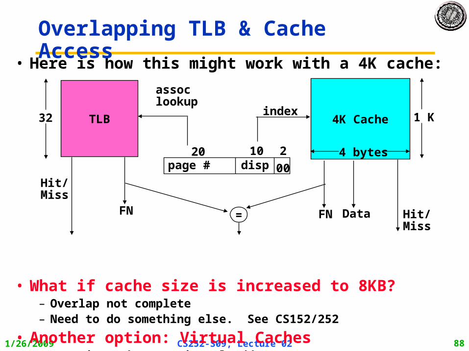
• Here is how this might work with a 4K cache:
• What if cache size is increased to 8KB?– Overlap not complete– Need to do something else. See CS152/252
• Another option: Virtual Caches– Tags in cache are virtual addresses– Translation only happens on cache misses
TLB 4K Cache
10 2
004 bytes
index 1 K
page # disp20
assoclookup
32
Hit/Miss
FN Data Hit/Miss
=FN
Overlapping TLB & Cache Access
1/26/2009 CS252-S09, Lecture 02 89
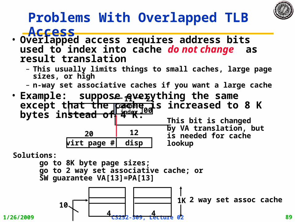
Problems With Overlapped TLB Access
11 2
00
virt page # disp20 12
cache index
This bit is changedby VA translation, butis needed for cachelookup
Solutions: go to 8K byte page sizes; go to 2 way set associative cache; or SW guarantee VA[13]=PA[13]
1K
4 410
2 way set assoc cache
• Overlapped access requires address bits used to index into cache do not change as result translation
– This usually limits things to small caches, large page sizes, or high– n-way set associative caches if you want a large cache
• Example: suppose everything the same except that the cache is increased to 8 K bytes instead of 4 K:

1/26/2009 CS252-S09, Lecture 02 90
Summary: Control and Pipelining• Next time: Read Appendix A
• Control VIA State Machines and Microprogramming
• Just overlap tasks; easy if tasks are independent
• Speed Up Pipeline Depth; if ideal CPI is 1, then:
• Hazards limit performance on computers:– Structural: need more HW resources
– Data (RAW,WAR,WAW): need forwarding, compiler scheduling
– Control: delayed branch, prediction
• Exceptions, Interrupts add complexity
• Next time: Read Appendix C, record bugs online!
pipelined
dunpipeline
TimeCycle
TimeCycle
CPI stall Pipeline 1depth Pipeline
Speedup
1/26/2009 CS252-S09, Lecture 02 91
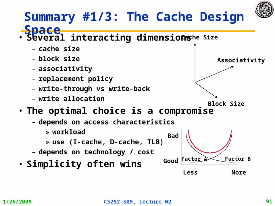
Summary #1/3: The Cache Design Space• Several interacting dimensions
– cache size
– block size
– associativity
– replacement policy
– write-through vs write-back
– write allocation
• The optimal choice is a compromise– depends on access characteristics
» workload
» use (I-cache, D-cache, TLB)
– depends on technology / cost
• Simplicity often wins
Associativity
Cache Size
Block Size
Bad
Good
Less More
Factor A Factor B

1/26/2009 CS252-S09, Lecture 02 92
Summary #2/3: Caches• The Principle of Locality:
– Program access a relatively small portion of the address space at any instant of time.
» Temporal Locality: Locality in Time» Spatial Locality: Locality in Space
• Three Major Categories of Cache Misses:– Compulsory Misses: sad facts of life. Example: cold start misses.– Capacity Misses: increase cache size– Conflict Misses: increase cache size and/or associativity.
Nightmare Scenario: ping pong effect!
• Write Policy: Write Through vs. Write Back• Today CPU time is a function of (ops, cache misses)
vs. just f(ops): affects Compilers, Data structures, and Algorithms
1/26/2009 CS252-S09, Lecture 02 93
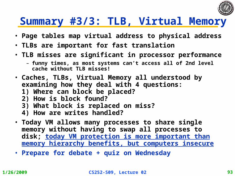
Summary #3/3: TLB, Virtual Memory• Page tables map virtual address to physical address
• TLBs are important for fast translation
• TLB misses are significant in processor performance– funny times, as most systems can’t access all of 2nd level cache without
TLB misses!
• Caches, TLBs, Virtual Memory all understood by examining how they deal with 4 questions: 1) Where can block be placed?2) How is block found? 3) What block is replaced on miss? 4) How are writes handled?
• Today VM allows many processes to share single memory without having to swap all processes to disk; today VM protection is more important than memory hierarchy benefits, but computers insecure
• Prepare for debate + quiz on Wednesday