EE516 { Speech Processing and...
53
EE516 – Speech Processing and Recognition — Spring Quarter, Lecture 9 — http://j.ee.washington.edu/ ~ bilmes/classes/ee516_spring_2015/ Prof. Jeff Bilmes University of Washington, Seattle Department of Electrical Engineering http://melodi.ee.washington.edu/ ~ bilmes May 25th, 2015 Prof. Jeff Bilmes EE516/Spring 2015/Speech Proc - Lecture 9 - May 25th, 2015 F1/102 (pg.1/105) Logistics Review Announcements, Assignments, and Reminders Office hours google hangouts (watch email for links, success!!). Prof: Office hours now Wednesdays 8-9pm via google hangout link above. TA: Yuzong Liu [email protected]. TA: office hours, Thursdays 7pm via google hangouts link above. Discussion on google hangouts vs. skype. Prof. Jeff Bilmes EE516/Spring 2015/Speech Proc - Lecture 9 - May 25th, 2015 F2/102 (pg.2/105)
Transcript of EE516 { Speech Processing and...

EE516 – Speech Processing and Recognition— Spring Quarter, Lecture 9 —
http://j.ee.washington.edu/~bilmes/classes/ee516_spring_2015/
Prof. Jeff Bilmes
University of Washington, SeattleDepartment of Electrical Engineering
http://melodi.ee.washington.edu/~bilmes
May 25th, 2015
Prof. Jeff Bilmes EE516/Spring 2015/Speech Proc - Lecture 9 - May 25th, 2015 F1/102 (pg.1/105)
Logistics Review
Announcements, Assignments, and Reminders
Office hours google hangouts (watch email for links, success!!).
Prof: Office hours now Wednesdays 8-9pm via google hangout linkabove.
TA: Yuzong Liu [email protected].
TA: office hours, Thursdays 7pm via google hangouts link above.
Discussion on google hangouts vs. skype.
Prof. Jeff Bilmes EE516/Spring 2015/Speech Proc - Lecture 9 - May 25th, 2015 F2/102 (pg.2/105)

Logistics Review
Homework/Final Project
The final project will consist of writing in Matlab from scratch asimple speaker dependent, isolated-word, whole-word model (i.e., oneHMM/word), single Gaussian per state, diagonal covariance Gaussian,speech recognition system, using the five-word vocabulary “zero”,“one”, “two”, “three”, and “four”
By Monday, May 25nd, you need to write code to produce MFCCs(homework 4).
By Next Monday, June 1st, you need to write code to train GaussianHMMs on your MFCCs (you dont’ need to do mixtures). (homework5).
By Monday, June 8th, your code should be fully working anddebugged also, you’ll be demoing your system in class on a laptop(final project) both with your own speech and one other person. Alsowhen you need to turn in a 1-2 page writeup on your project.
Prof. Jeff Bilmes EE516/Spring 2015/Speech Proc - Lecture 9 - May 25th, 2015 F3/102 (pg.3/105)
Logistics Review
Review
Delta Speech Features, and double deltas
The Trellis, and trellis structures vs. transition matrices
HMM α,β recursions, and the γ and ξ quantities, efficientcomputation.
Prof. Jeff Bilmes EE516/Spring 2015/Speech Proc - Lecture 9 - May 25th, 2015 F4/102 (pg.4/105)

Logistics Review
Good books (for today)
our book (Huang, Acero, Hon, “Spoken Language Processing”)Rabiner&Juang: Fundamentals of speech recognition.Deller et. al. “Discrete-time Processing of speech signals”O’Shaughnessy, “Speech Communications”J. Bilmes, “What HMMs can do”, 2010
Prof. Jeff Bilmes EE516/Spring 2015/Speech Proc - Lecture 9 - May 25th, 2015 F5/102 (pg.5/105)
HMM ASR structure, and training data Learning HMMs
Transition matrix structure
A matrix Markov chain topology (where zeros are) is crucial for goodperformance.
Most common: strictly left-to-right (used for sub-word sequences):
/c/ /a/ /a/ /t/
Generally: upper triangular:
aij = 0 for j < i (9.1)
aNN = 1, aNi = 0 (9.2)
a11 = 0, a12 = 1, a1j = 0, j > 2 (9.3)
L2R property of matrix also helps discriminability === ability todistinguish one sound from another. More on this when we coverdiscriminative training.
Prof. Jeff Bilmes EE516/Spring 2015/Speech Proc - Lecture 9 - May 25th, 2015 F6/102 (pg.6/105)

HMM ASR structure, and training data Learning HMMs
HMM Training: Collecting Data
One of the benefits of HMMs is that there are formal procedures fortraining them.
We will very soon discuss two general approaches, the EM algorithm(generative training under the maximum likelihood criterion), anddiscriminative training approaches.
In either case, it is necessary to have training data.
Prof. Jeff Bilmes EE516/Spring 2015/Speech Proc - Lecture 9 - May 25th, 2015 F7/102 (pg.7/105)
HMM ASR structure, and training data Learning HMMs
HMM Training: Forms of Data
Training data D ={
(x(i)1:Ti
, w(i))}i, where x
(i)1:Ti
is a matrix of speech
features and w(i) is the set of labels (word transcription) of speech.
Unsupervised training data: when one has only Du ={x
(i)1:Ti
}i
Semi-supervised training data: when one has only Du ={x
(i)1:Ti
}i
and
Ds ={
(x(i)1:Ti
, w(i))}j.
Extra language data D` ={w(i)
}j
useful since HMMs are generativemodels. Acoustic and language data can have little overlap.
Language data can be either: 1) sequence of words, 2) sequence ofwords where center time-mark is known, and 3) sequence of wordswhere word boundaries are known.
Prof. Jeff Bilmes EE516/Spring 2015/Speech Proc - Lecture 9 - May 25th, 2015 F8/102 (pg.8/105)

HMM ASR structure, and training data Learning HMMs
HMM Training: Forms of Data
Training data D ={
(x(i)1:Ti
, w(i))}i, where x
(i)1:Ti
is a matrix of speech
features and w(i) is the set of labels (word transcription) of speech.
Unsupervised training data: when one has only Du ={x
(i)1:Ti
}i
Semi-supervised training data: when one has only Du ={x
(i)1:Ti
}i
and
Ds ={
(x(i)1:Ti
, w(i))}j.
Extra language data D` ={w(i)
}j
useful since HMMs are generativemodels. Acoustic and language data can have little overlap.
Language data can be either: 1) sequence of words, 2) sequence ofwords where center time-mark is known, and 3) sequence of wordswhere word boundaries are known.
Prof. Jeff Bilmes EE516/Spring 2015/Speech Proc - Lecture 9 - May 25th, 2015 F9/102 (pg.9/105)
HMM ASR structure, and training data Learning HMMs
Supervised Speech Data
Collecting quality training data is time consuming, error prone,difficult, and expensive.
Big clean data has been critical to the recent successes ofbig-company ASR systems.
Lets assume supervised case: D ={
(x(i)1:Ti
, w(i))}i, where x
(i)1:Ti
is a
matrix of speech features and w(i) is the set of labels (wordtranscription) of speech.
Prof. Jeff Bilmes EE516/Spring 2015/Speech Proc - Lecture 9 - May 25th, 2015 F10/102 (pg.10/105)

HMM ASR structure, and training data Learning HMMs
Speech data - vocabulary size
In (x(i)1:Ti
, w(i)), x1:Ti is a sequence of length Ti and w(i) is a sequencealso of variable length (length Ni).
Vocabulary size (also called lexicon size, or number of types) is key —the bigger the vocabulary, the harder the problem becomes
This is an issue of confusability.
10 word vocabulary is much less confusable than 250,000 wordvocabulary, much more likely that two words are almost the same asvocabulary increases.
Prof. Jeff Bilmes EE516/Spring 2015/Speech Proc - Lecture 9 - May 25th, 2015 F11/102 (pg.11/105)
HMM ASR structure, and training data Learning HMMs
Speech data - types of speech systems and supporting data
Carefully read speech vs. continuous speech (with disfluencies).
Noise condition (how noisy is the speech) - high SNR is much easierthan low SNR.
Accent, dialect, code switching (mixed languages), idiolect, childspeech, age-specific characteristics,
Isolated word ASR (silence between each speech unit, or between eachword) vs. “continuous” speech (no clear boundary between words).
Key words of wisdom: to develop a system of a particular type, oneneeds lots of supporting training data (many examples of every kind ofidiosyncratic speech characteristic).
Prof. Jeff Bilmes EE516/Spring 2015/Speech Proc - Lecture 9 - May 25th, 2015 F12/102 (pg.12/105)

HMM ASR structure, and training data Learning HMMs
Speech data - what is in the lexicon
w(i) = (w(i)1 , w
(i)2 , . . . , w
(i)Ni
) is a ordered list of lexical items, but whatare they?
Conversational speech: filled with disfluencies!
From Wikipedia:
A speech disfluency . . . is any of various breaks, irregularities,or non-lexical vocables that occurs within the flow ofotherwise fluent speech. These include false starts, i.e.words and sentences that are cut off mid-utterance, phrasesthat are restarted or repeated and repeated syllables, fillersi.e. grunts or non-lexical utterances such as “uh”, “erm”and “well”, and repaired utterances, i.e. instances ofspeakers correcting their own slips of the tongue ormispronunciations (before anyone else gets a chance to).
Prof. Jeff Bilmes EE516/Spring 2015/Speech Proc - Lecture 9 - May 25th, 2015 F13/102 (pg.13/105)
HMM ASR structure, and training data Learning HMMs
Speech Disfluency Typeshttp://www.is.cs.cmu.edu/11-733/2003/Slides/FeiHuang.pdf
Name Abbrev. Description Example
Repetition orcorrection
REP
Exact repetition or correctionof words previously uttered.A correction may involve sub-stitutions, deletions, or in-sertions of words. Correc-tion continues with the sameidea/train of thought startedpreviously.
If I can’t find don’t knowthe answer myself, I willfind it. If if nobodywants to influence Presi-dent Clinton
False Start FSAn utterance is aborted andrestarted with a new idea ortrain of thought
We’ll never find whatabout next month?
Filled Pause UHAll other filler words perhapswith little (or non-obvious)semantic content
yeah, oh, okay etc.
Interjection IN
Restricted group of non-lexicalized sounds indicatingaffirmation or negation. E.g.,back-channeling, sometimeswith no obvious semanticcontent.
uh-huh, mmm, umm, uh-uh
Prof. Jeff Bilmes EE516/Spring 2015/Speech Proc - Lecture 9 - May 25th, 2015 F14/102 (pg.14/105)

HMM ASR structure, and training data Learning HMMs
Speech Disfluency Typeshttp://www.is.cs.cmu.edu/11-733/2003/Slides/FeiHuang.pdf
Name Abbrev. Description Example
Editing Term ET
Phrases that occur be-tween that part of a dis-fluency which will be cor-rected and the actual re-pair. They refer explicitlyto the words that just pre-viously have been said in-dicating that they will beedited.
We need two tickets, I’msorry three tickets for theflight to Boston.
DiscourseMarker
DM
Words that are related tothe structure of the dis-course in so far that theyhelp beginning or keepinga turn or serve no acknowl-edgment. They do notcontribute to the semanticcontent of the dialogue.
Well this is a good idea.This is, you know, a prettygood solution to our prob-lem.
Prof. Jeff Bilmes EE516/Spring 2015/Speech Proc - Lecture 9 - May 25th, 2015 F15/102 (pg.15/105)
HMM ASR structure, and training data Learning HMMs
Statistics about Disfluencies
Estimations exist of the following (see the work of Liz Schriberg for moredetails).
The number of disfluency per sentence grow linearly with sentencelength.
The number of fluent sentences decrease exponentially over thesentence length.
Disfluencies are not distributed uniformly over positions.
The frequency of disfluency decreases exponentially w.r.t. its length(number of words).
Prof. Jeff Bilmes EE516/Spring 2015/Speech Proc - Lecture 9 - May 25th, 2015 F16/102 (pg.16/105)

HMM ASR structure, and training data Learning HMMs
Speech data — speech annotation
Repetition/correction/restart/filler: What do these sound like?
How are they annotated in trained data?
Annotating speech data (taking x and producing labels w) is difficult.
Time it takes to do this is many times real time.
There is no universal agreement —- word boundaries are ambiguous.
Prof. Jeff Bilmes EE516/Spring 2015/Speech Proc - Lecture 9 - May 25th, 2015 F17/102 (pg.17/105)
HMM ASR structure, and training data Learning HMMs
Word boundaries are ambiguous
Spectra of cuttings obtained from Switchboard conversation sw02423.cutting the B-channel from 1:44:741s to 1:45:704s . The arrows showword boundaries hypothesized by trained speech researchers asked toannotate these cuttings.
Prof. Jeff Bilmes EE516/Spring 2015/Speech Proc - Lecture 9 - May 25th, 2015 F18/102 (pg.18/105)

HMM ASR structure, and training data Learning HMMs
Word boundaries are ambiguous
Spectra of cuttings obtained from Switchboard conversation sw02423.cutting the A-channel from 8:05:530s to 8:06:622s. The arrows showword boundaries hypothesized by trained speech researchers asked toannotate these cuttings.
Prof. Jeff Bilmes EE516/Spring 2015/Speech Proc - Lecture 9 - May 25th, 2015 F18/102 (pg.19/105)
HMM ASR structure, and training data Learning HMMs
Speech data — prosody
What to do about prosody?
Suprasegmental: effects extend beyond the phoneme into units ofsyllables, words, phrases, and sometimes even sentence.
Prosody: perception of rhythm, intonation, and stress patterns —helps the listener understand the speech message by pointing outimportant words and by cueing logical breaks in the flow of anutterance.
Helps mentally process speech,
Determines message: “Joe has studied”, is it a question or astatement, depends on prosody.
Dialog acts, reflect the functions that an utterance serves in adiscourse (questions, statements, back-channels, )
Prof. Jeff Bilmes EE516/Spring 2015/Speech Proc - Lecture 9 - May 25th, 2015 F19/102 (pg.20/105)

HMM ASR structure, and training data Learning HMMs
Dialog acts
Dialog acts (speech acts) group families of surface utterances intofunctional classes.
Directive: The speaker wants the listener to do something.
Commissive: The speaker indicates that s/he herself will do somethingin future.
Expressive: The speaker expresses his or her feelings or emotionalresponse.
Representative: The speaker expresses his or her belief about the truthof a proposition.
Declarative: Speaker’s utterance causes a change in external,nonlinguistic situation.
Should these be annotated as well?
Prof. Jeff Bilmes EE516/Spring 2015/Speech Proc - Lecture 9 - May 25th, 2015 F20/102 (pg.21/105)
HMM ASR structure, and training data Learning HMMs
Rich annotation/Rich Transcription
Rather than just the words, we might augment lexicon with a widevariety of other aspects of the speech signal.
Some might occur concurrently with the words, so really w(i) might bea list of discrete vectors (i.e., at any time, we have a word, a certaintyabout a word boundary, a dialog act, a prosodic category, etc.)
Above is a “shallow parse” of the speech signal, but highergrammatical structure we might also wish to infer.
This makes both the human transcriber’s job and the speechrecognizers job much harder.
Prof. Jeff Bilmes EE516/Spring 2015/Speech Proc - Lecture 9 - May 25th, 2015 F21/102 (pg.22/105)

HMM ASR structure, and training data Learning HMMs
Speech data — text normalization
One last item is that the same utterances need to be annotated thesame way.
We need to normalize the text so that punctuation, stress marks,indications of disfluency are the same.
Text normalization: conversion from the variety symbols, numbers,and other nonorthographic entities of text into a commonorthographic transcription suitable for subsequent phonetic conversion.
Normally done on text corpora where end-of-sentence detection, theexpansion of abbreviations, and the treatment of acronyms andnumbers, is necessary to make the text processable in a unified way.
Annotator differences, different annotators should ideally do the samething, need to normalize in the same way.
Prof. Jeff Bilmes EE516/Spring 2015/Speech Proc - Lecture 9 - May 25th, 2015 F22/102 (pg.23/105)
HMM ASR structure, and training data Learning HMMs
Supervised Speech Data
Collecting quality training data is time consuming, error prone,difficult, and expensive.
Big clean data has been critical to the recent successes ofbig-company ASR systems.
Lets assume supervised case: D ={
(x(i)1:Ti
, w(i))}i, where x
(i)1:Ti
is a
matrix of speech features and w(i) is the set of labels (wordtranscription) of speech.
Prof. Jeff Bilmes EE516/Spring 2015/Speech Proc - Lecture 9 - May 25th, 2015 F23/102 (pg.24/105)

HMM ASR structure, and training data Learning HMMs
HMM: As factorization
Using the conditional independence statements mentioned above, we canderive the following factorization:
p(x1:T , q1:T ) = p(xT , qT |x1:T−1, q1:T−1)p(x1:T−1, q1:T−1) (9.21)
= p(xT |qT , x1:T−1, q1:T−1)p(qT |x1:T−1, q1:T−1) (9.22)
p(x1:T−1, q1:T−1) (9.23)
= p(xT |qT )p(qT |qT−1)p(x1:T−1, q1:T−1) (9.24)
= . . . (9.25)
= p(q1)
T∏t=2
p(qt|qt−1)
T∏t=1
p(xt|qt) (9.26)
This last equation is the classical factorization expression for an HMMjoint distribution over x1:T , q1:T .
Prof. Jeff Bilmes EE516/Spring 2015/Speech Proc - Lecture 9 - May 25th, 2015 F24/102 (pg.25/105)
HMM ASR structure, and training data Learning HMMs
HMM parameters
Parameters of HMM, depend on nature of underlying Markov chain.
If time-homogeneous, we have an initial state distribution (typically π)with p(Q1 = i) = πi, and a state transition matrix A.
We also have the set of observation distributionsbj(x) = p(Xt = x|Qt = j) in the time-homogeneous case. In timehomogeneous case, we might have bt,j(x). Also, B = {bi(·)}i.HMM, conditional on parameters λ, is given as p(x1:T |λ).
All three parameters (initial distribution, transition matrix, andobservation distribution) together refer to using λ = (π,A,B).
Sampling from an HMM means: 1) first randomly choose anassignment to Q1:T and then 2) randomly choose an assignment toX1:T given Q1:T .
Each new X sample requires a new Q sample.
Prof. Jeff Bilmes EE516/Spring 2015/Speech Proc - Lecture 9 - May 25th, 2015 F25/102 (pg.26/105)

HMM ASR structure, and training data Learning HMMs
Speech Data
We train on all of the data D ={
(x(i)1:Ti
, w(i))}i, but notationally it is
sometimes easy to assume we have only one utterance sample that isvery long.
Prof. Jeff Bilmes EE516/Spring 2015/Speech Proc - Lecture 9 - May 25th, 2015 F26/102 (pg.27/105)
HMM ASR structure, and training data Learning HMMs
Parameter Training
Still two problems to solve.
Problem 3: Maximum Likelihood Training
Problem 4: Discriminative Training (next week)
Why not just do:
∂
∂λpλ(x1:T |M) = 0 (9.4)
and then solve for λ?
Recall in an HMM:
p(x1:T ) =∑q1:T
∏t
p(xt|qt)p(qt|qt−1) (9.5)
Parameters are “coupled”, no closed form solution since sums do notdistribute into products with separate parameters (parameters for eachfactor are “dependent” on each other).
Prof. Jeff Bilmes EE516/Spring 2015/Speech Proc - Lecture 9 - May 25th, 2015 F27/102 (pg.28/105)

HMM ASR structure, and training data Learning HMMs
Parameter Training
Could continue with derivatives, and iterate with old to produce new,but does this converge?
EM algorithm helps with this. Missing data consists of hidden variableassignments, take expected full log likelihood conditioned on data anda “previous” guess of the parameters, and then iterate.
Prof. Jeff Bilmes EE516/Spring 2015/Speech Proc - Lecture 9 - May 25th, 2015 F28/102 (pg.29/105)
HMM ASR structure, and training data Learning HMMs
HMM - learning with EM
To decide which queries to compute, should know which ones we want.If learning HMM parameters with EM, what queries do we need?
X1:T = x1:T observed, Q1:T hidden variables, λ are parameters tolearn, and λg are the previous iteration parameters. EM thenrepeatedly optimizes the following objective:
Prof. Jeff Bilmes EE516/Spring 2015/Speech Proc - Lecture 9 - May 25th, 2015 F29/102 (pg.30/105)

HMM ASR structure, and training data Learning HMMs
HMM - learning with EM
We use an auxiliary function Q(λ, λg) which is a function only of λ:
f(λ) = Q(λ, λg) (9.6)
= Ep(x1:T ,q1:T |λg)[log p(x1:T , q1:T |λ)] (9.7)
=∑q1:T
p(x1:T , q1:T |λg)[log p(x1:T , q1:T |λ)] (9.8)
= Ep[log∏t
p(qt|qt−1, λ)p(xt|qt, λ)] (9.9)
= Ep[∑t
log p(qt|qt−1, λ) +∑t
log p(xt|qt, λ)] (9.10)
=(∑
t
∑ij
p(Qt = j,Qt−1 = i|x1:T , λg) log p(Qt = j|Qt−1 = i, λ)
+∑t
∑i
p(Qt = i|x1:T , λg) log p(xt|Qt = i, λ)
)(9.11)
p(x1:T |λg) (9.12)
Prof. Jeff Bilmes EE516/Spring 2015/Speech Proc - Lecture 9 - May 25th, 2015 F30/102 (pg.31/105)
HMM ASR structure, and training data Learning HMMs
Distributive law and marginal probabilities
The above follows for the same reasons as the below follows:∑q1:T
p(q1:T )[f1(q1, q2) + f2(q2, q3)] (9.13)
=∑q1:T
p(q1:T )f1(q1, q2) +∑q1:T
p(q1:T )f2(q2, q3) (9.14)
=∑q1,q2
f1(q1, q2)∑q3:T
p(q1:T ) +∑q2,q3
f2(q2, q3)∑q1,4:T
p(q1:T ) (9.15)
=∑q1,q2
f1(q1, q2)p(q1, q2) +∑q2,q3
f2(q2, q3)p(q2, q3) (9.16)
Prof. Jeff Bilmes EE516/Spring 2015/Speech Proc - Lecture 9 - May 25th, 2015 F31/102 (pg.32/105)
HMM ASR structure, and training data Learning HMMs
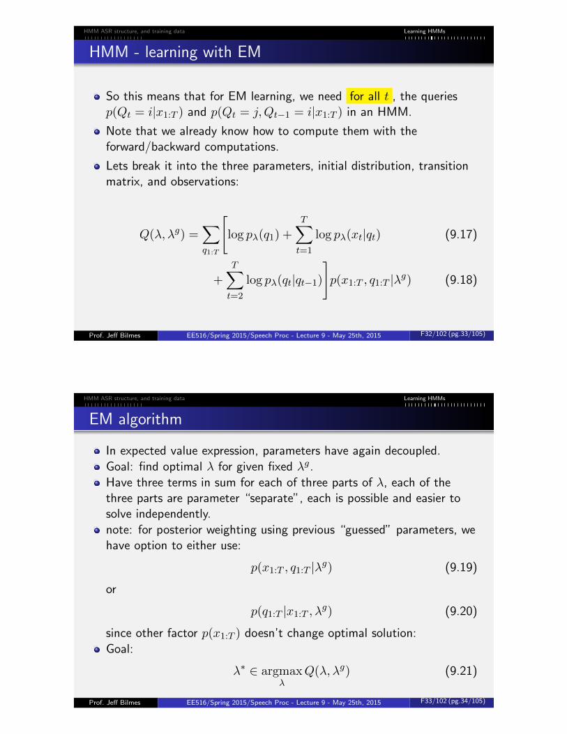
HMM - learning with EM
So this means that for EM learning, we need for all t , the queriesp(Qt = i|x1:T ) and p(Qt = j,Qt−1 = i|x1:T ) in an HMM.
Note that we already know how to compute them with theforward/backward computations.
Lets break it into the three parameters, initial distribution, transitionmatrix, and observations:
Q(λ, λg) =∑q1:T
[log pλ(q1) +
T∑t=1
log pλ(xt|qt) (9.17)
+
T∑t=2
log pλ(qt|qt−1)
]p(x1:T , q1:T |λg) (9.18)
Prof. Jeff Bilmes EE516/Spring 2015/Speech Proc - Lecture 9 - May 25th, 2015 F32/102 (pg.33/105)
HMM ASR structure, and training data Learning HMMs
EM algorithm
In expected value expression, parameters have again decoupled.Goal: find optimal λ for given fixed λg.Have three terms in sum for each of three parts of λ, each of thethree parts are parameter “separate”, each is possible and easier tosolve independently.note: for posterior weighting using previous “guessed” parameters, wehave option to either use:
p(x1:T , q1:T |λg) (9.19)
or
p(q1:T |x1:T , λg) (9.20)
since other factor p(x1:T ) doesn’t change optimal solution:Goal:
λ∗ ∈ argmaxλ
Q(λ, λg) (9.21)
Prof. Jeff Bilmes EE516/Spring 2015/Speech Proc - Lecture 9 - May 25th, 2015 F33/102 (pg.34/105)

HMM ASR structure, and training data Learning HMMs
EM - initial state, p(q1), π
We optimize first term:∑q1:T
log pλ(q1)p(x1:T , q1:T |λg) =∑q1
log pλ(q1)p(x1:T , q1|λg) (9.22)
Need to stay within probability simplex, so use Lagrange multiplier α
α(∑q1
pλ(q1)− 1) (9.23)
get:
∂
∂πj
(∑i
log πip(x1:T , Q1 = i|λg) + α(∑i
πi − 1))
= 0 (9.24)
or
1
πjp(x1:T , Q1 = j|λg) + α = 0 (9.25)
Prof. Jeff Bilmes EE516/Spring 2015/Speech Proc - Lecture 9 - May 25th, 2015 F34/102 (pg.35/105)
HMM ASR structure, and training data Learning HMMs
EM - initial state, p(q1), π
This gives
απj = −p(x1:T , Q1 = j|λg) (9.26)
Then using:
∂
∂α
(∑i
log πip(x1:T , Q1 = i|λg) + α(∑i
πi − 1))
= 0 (9.27)
Gives
α∑j
πj = −∑j
p(x1:T , Q1 = j|λg) (9.28)
Or
α = −p(x1:T |λg) (9.29)
Prof. Jeff Bilmes EE516/Spring 2015/Speech Proc - Lecture 9 - May 25th, 2015 F35/102 (pg.36/105)

HMM ASR structure, and training data Learning HMMs
EM - initial state, p(q1), π
This gives the solution for the first term:
πj =p(x1:T , Q1 = j|λg)
p(x1:T |λg)= p(Q1 = j|λg, x1:T ) (9.30)
Again, we may easily compute this using α, β as follows:
p(Q1 = j|λg, x1:T ) =αj(1)βj(1)∑q αq(1)βq(1)
(9.31)
Multiple utterances: When there are L utterances, x`1:T`is the `th
utterance, x`t is tth frame of the `th utterance, T` is the number offrames of the `th utterance, we have:
πj =
∑L`=1 p(Q1 = j|λg, x`1:T`
)
L=
1
L
L∑`=1
α`j(1)β`j(1)∑q α
`q(1)β`q(1)
(9.32)
where α`j(1) and β`j(1) are the corresponding α and β quantity from
the `th utterance.Prof. Jeff Bilmes EE516/Spring 2015/Speech Proc - Lecture 9 - May 25th, 2015 F36/102 (pg.37/105)
HMM ASR structure, and training data Learning HMMs
EM - state-transition matrix aij
To optimize the state transition matrix [A]ij = aij
∑q1:T
[ T∑t=2
log pλ(qt|qt−1)]p(x1:T , q1:T |λg) (9.33)
=
N∑i=1
n∑j=1
T∑t=2
log pλ(j|i)p(x1:T , Qt−1 = i, Qt = j|λg) (9.34)
Using Lagrange multipliers again (for the transition probabilities, onefor each row), we get the solution:
aij =
∑Tt=2 p(x1:T , Qt−1 = i, Qt = j|λg)∑T
t=2 p(x1:T , Qt−1 = i|λg)(9.35)
Prof. Jeff Bilmes EE516/Spring 2015/Speech Proc - Lecture 9 - May 25th, 2015 F37/102 (pg.38/105)

HMM ASR structure, and training data Learning HMMs
EM - state-transition matrix aij
We saw last time that this was easily computable, again from the αand β quantities, namely
ξi,j(t− 1) =βt(j)a
gi,jp(xt|Qt = j)αt−1(i)
p(x1:T |λg)(9.36)
Thus, we get:
aij =
∑Tt=2 ξij(t)∑Tt=2 γi(t)
=expected number transitions from i to j
expected number of times in state i
(9.37)
Prof. Jeff Bilmes EE516/Spring 2015/Speech Proc - Lecture 9 - May 25th, 2015 F38/102 (pg.39/105)
HMM ASR structure, and training data Learning HMMs
EM - state-transition matrix aij, multiple utterances
When there are L utterances, x`1:T`is the `th utterance, x`t is tth frame
of the `th utterance, T` is the number of frames of the `th utterance,we have:
aij =
∑L`=1
∑T`t=2 p(Qt−1 = i, Qt = j|x`1:T`
, λg)∑L`=1
∑T`t=2 p(Qt−1 = i|x`1:T`
, λg)(9.38)
=
∑L`=1
∑T`t=2 ξ
`ij(t)∑L
`=1
∑T`t=2 γ
`i (t)
(9.39)
where ξ`ij(t) and γ`i (t) are the corresponding quantities computing
from the `th utterance, implying that each utterance must have itsown separate α` and β` quantities.
Prof. Jeff Bilmes EE516/Spring 2015/Speech Proc - Lecture 9 - May 25th, 2015 F39/102 (pg.40/105)
HMM ASR structure, and training data Learning HMMs
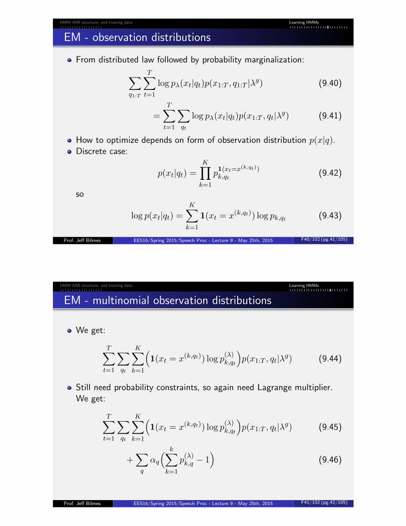
EM - observation distributions
From distributed law followed by probability marginalization:∑q1:T
T∑t=1
log pλ(xt|qt)p(x1:T , q1:T |λg) (9.40)
=
T∑t=1
∑qt
log pλ(xt|qt)p(x1:T , qt|λg) (9.41)
How to optimize depends on form of observation distribution p(x|q).Discrete case:
p(xt|qt) =
K∏k=1
p1(xt=x(k,qt))k,qt
(9.42)
so
log p(xt|qt) =
K∑k=1
1(xt = x(k,qt)) log pk,qt (9.43)
Prof. Jeff Bilmes EE516/Spring 2015/Speech Proc - Lecture 9 - May 25th, 2015 F40/102 (pg.41/105)
HMM ASR structure, and training data Learning HMMs
EM - multinomial observation distributions
We get:
T∑t=1
∑qt
K∑k=1
(1(xt = x(k,qt)) log p
(λ)k,qt
)p(x1:T , qt|λg) (9.44)
Still need probability constraints, so again need Lagrange multiplier.We get:
T∑t=1
∑qt
K∑k=1
(1(xt = x(k,qt)) log p
(λ)k,qt
)p(x1:T , qt|λg) (9.45)
+∑q
αq
( k∑k=1
p(λ)k,q − 1
)(9.46)
Prof. Jeff Bilmes EE516/Spring 2015/Speech Proc - Lecture 9 - May 25th, 2015 F41/102 (pg.42/105)
HMM ASR structure, and training data Learning HMMs
EM - multinomial observation distributions
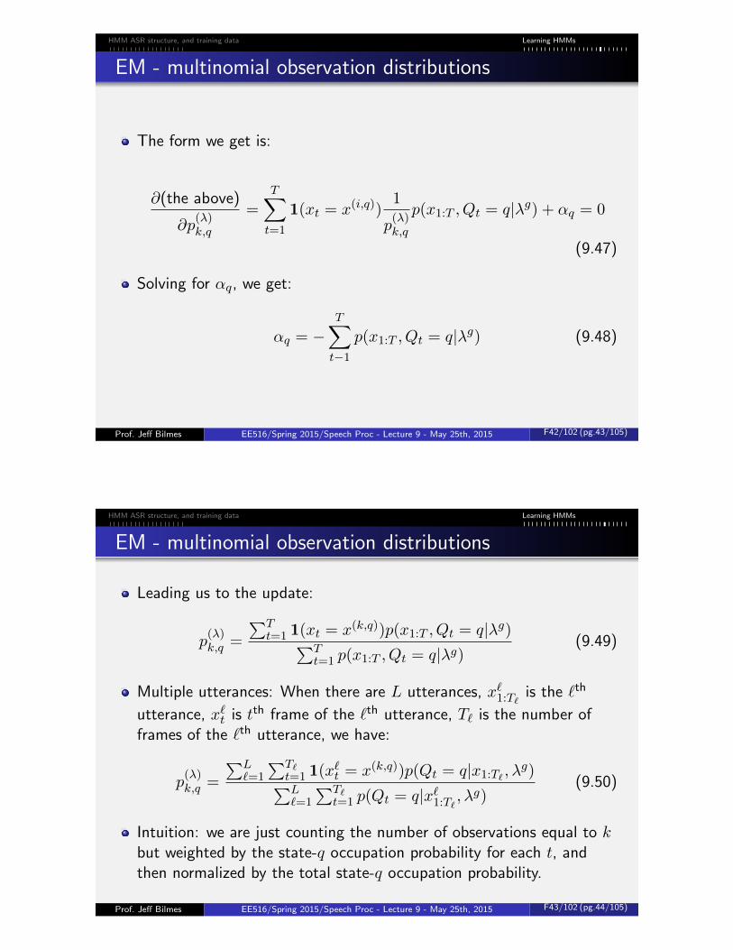
The form we get is:
∂(the above)
∂p(λ)k,q
=T∑t=1
1(xt = x(i,q))1
p(λ)k,q
p(x1:T , Qt = q|λg) + αq = 0
(9.47)
Solving for αq, we get:
αq = −T∑t−1
p(x1:T , Qt = q|λg) (9.48)
Prof. Jeff Bilmes EE516/Spring 2015/Speech Proc - Lecture 9 - May 25th, 2015 F42/102 (pg.43/105)
HMM ASR structure, and training data Learning HMMs
EM - multinomial observation distributions
Leading us to the update:
p(λ)k,q =
∑Tt=1 1(xt = x(k,q))p(x1:T , Qt = q|λg)∑T
t=1 p(x1:T , Qt = q|λg)(9.49)
Multiple utterances: When there are L utterances, x`1:T`is the `th
utterance, x`t is tth frame of the `th utterance, T` is the number offrames of the `th utterance, we have:
p(λ)k,q =
∑L`=1
∑T`t=1 1(x`t = x(k,q))p(Qt = q|x1:T` , λ
g)∑L`=1
∑T`t=1 p(Qt = q|x`1:T`
, λg)(9.50)
Intuition: we are just counting the number of observations equal to kbut weighted by the state-q occupation probability for each t, andthen normalized by the total state-q occupation probability.
Prof. Jeff Bilmes EE516/Spring 2015/Speech Proc - Lecture 9 - May 25th, 2015 F43/102 (pg.44/105)

HMM ASR structure, and training data Learning HMMs
EM - multivariate Gaussian distributions
In a multivariate Gaussian HMM, each state is associated with amultivariate Gaussian density. Let qt be a state variable at time t.Then p(xt|qt) is a multivariate Gaussian, where the Gaussian isindexed by the identify of the state qt ∈ {1, 2, . . . ,M}, where M isthe number of states in the HMM.A multivariate Gaussian takes the following mathematical form:
p(xt|qt) =1√|2πCqt |
exp
(−1
2(xt − µqt)ᵀC−1
qt (xt − µqt))
(9.51)
where µqt ∈ RN is an N -dimensional real vector, and Cqt ∈ RN×N isa positive definite matrix.We often just use a diagonal covariance matrix, so thatCqt = diag(Cqt).Hence, the set of Gaussians is characterized by a set of N meanvectors and N covariance matrices.Typically, in real systems Gaussian mixtures (or deep neural networks)are used for each HMM state.
Prof. Jeff Bilmes EE516/Spring 2015/Speech Proc - Lecture 9 - May 25th, 2015 F44/102 (pg.45/105)
HMM ASR structure, and training data Learning HMMs
EM - multivariate Gaussian distributions
For continuous densities (e.g., Gaussians) derivation is similar.
For a multivariate Gaussian for each state, we have a mean vector µqand covariance matrix Cq for each state.
Updates take the form:
µq =
∑Tt=1 xtp(x1:T , Qt = q|λg)∑Tt=1 p(x1:T , Qt = q|λg)
=
∑Tt=1 xtp(Qt = q|x1:T , λ
g)∑Tt=1 p(Qt = q|x1:T , λg)
(9.52)
and
Cq =
∑Tt=1(xt − µq)(xt − µq)ᵀp(x1:T , Qt = q|λg)∑T
t=1 p(x1:T , Qt = q|λg)(9.53)
So just weighted mean of vectors, or weighted mean of outer-products.
Q: how to do this in one pass through the data per epoch?
Prof. Jeff Bilmes EE516/Spring 2015/Speech Proc - Lecture 9 - May 25th, 2015 F45/102 (pg.46/105)

HMM ASR structure, and training data Learning HMMs
EM - multivariate Gaussians, multiple utterances
When there are L utterances, x`1:T`is the `th utterance, x`t is tth frame
of the `th utterance, T` is the number of frames of the `th utterance,we have the following update:
µq =
∑L`=1
∑T`t=1 x
`tp(Qt = q|x`1:T`
, λg)∑L`=1
∑T`t=1 p(Qt = q|x`1:T`
, λg)(9.54)
for the means, and
Cq =
∑L`=1
∑T`t=1(x`t − µq)(x`t − µq)
ᵀp(Qt = q|x`1:T`
, λg)∑L`=1
∑T`t=1 p(Qt = q|x`1:T`
, λg)(9.55)
for the covariance matrices.
Prof. Jeff Bilmes EE516/Spring 2015/Speech Proc - Lecture 9 - May 25th, 2015 F46/102 (pg.47/105)
HMM ASR structure, and training data Learning HMMs
EM iterations
Algorithm 1: EM algorithm, top-level iteration
input : Training data, auxiliary function Q(·, ·)input : Initial guess at the parameters λ0
1 i← 0 ;2 repeat3 i← i+ 1 ;4 λi ∈ argmaxλQ(λ, λi−1) ;
5 until log[p(x1:T |λi)/p(x1:T |λi−1)
]≤ τ (data log likelihood difference
falls below threshold);
Each iteration is often called an epoch
Goal is to maximize likelihood, i.e.:
λ∗ ∈ argmaxλ
log p(x1:T |λ) = argmaxλ
L(λ) (9.56)
Why does above iterative approach work?
Prof. Jeff Bilmes EE516/Spring 2015/Speech Proc - Lecture 9 - May 25th, 2015 F47/102 (pg.48/105)

HMM ASR structure, and training data Learning HMMs
EM - Why does it work?
Theorem 9.4.1
If Q(λ, λg) ≥ Q(λg, λg) then L(λ) ≥ L(λg) whereL(λ) = p(x1:T |λ) =
∑q1:T
p(x1:T , q1:T |λ) andQ(λ, λg) =
∑q1:T
p(q1:T |λg) log p(x1:T , q1:T |λ)
Proof.
log[L(λ)/L(λg)
]= log
[∑q1:T
p(x1:T , q1:T |λ)
L(λg)
](9.57)
= log
[∑q1:T
p(q1:T |λg, x1:T )
p(q1:T |λg, x1:T )
p(x1:T , q1:T |λ)
L(λg)
](9.58)
≥∑q1:T
p(q1:T |λg, x1:T ) logp(x1:T , q1:T |λ)
p(x1:T , q1:T |λg)(9.59)
= Q(λ, λg)−Q(λg, λg) ≥ 0 (9.60)
Prof. Jeff Bilmes EE516/Spring 2015/Speech Proc - Lecture 9 - May 25th, 2015 F48/102 (pg.49/105)
Words HMM Viterbi HMM Gradients Discriminative Training
HMMs and word sequences
HMM distribution p(x1:T , q1:T ) but what do states mean?
In speech, we have a hierarchy:
1 Sentences are composed of words.2 Words are composed of pronunciations, and can have multiple
pronunciations per word3 Word pronunciations are composed of phones.4 Phones are composed of subphones (e.g., triphones)5 Triphones are composed of low-level HMM states (triphone states).
We could treat this as a graphical model, where we have distinctrandom variables for each of the above levels.
In many HMM systems, however, the above hierarchy is “flattened”down into a single state variable and state sequence q1:T .
Hence, all of this needs somehow to be encoded in q1:T .
Prof. Jeff Bilmes EE516/Spring 2015/Speech Proc - Lecture 9 - May 25th, 2015 F49/102 (pg.50/105)

Words HMM Viterbi HMM Gradients Discriminative Training
HMMs and word sequences
In reality, a given state q ∈ DQ encodes all levels of the hierarchysimultaneously — ∃ a one-to-one mapping that (perhaps implicitly)performs the following relation:
q1:T ↔[(w1, . . . , wN ), (r1, . . . , rN ),((h1,1, . . . , h1,`1), (h2,1, . . . , h2,`2), . . . , (hN,1, . . . , hN,`N )
),(
(h′1,1, . . . , h′1,`1), (h′2,1, . . . , h
′2,`2), . . . , (h′N,1, . . . , h
′N,`N
)),(
(~y1,1, . . . , ~y1,`1), (~y2,1, . . . , ~y2,`2), . . . , (~yN,1, . . . , ~yN,`N ))]
where w1, . . . , wN is a sequence of words, r1, . . . , rN is a sequence ofword pronunciation ids, hi,1, . . . , hi,`i is a sequence of phones for wordpronunciation i, h′i,1, . . . , h
′i,`i
is a sequence of subphones for wordpronunciation i, and ~yi,j is a ordered vector of states (e.g., for atri-phone, three states, beginning/middle/end of the tri-phone).
Prof. Jeff Bilmes EE516/Spring 2015/Speech Proc - Lecture 9 - May 25th, 2015 F50/102 (pg.51/105)
Words HMM Viterbi HMM Gradients Discriminative Training
HMMs and word sequences
Hence, for a given word sequence w1, . . . , wN there can be manypossible states compatible with that word sequence.
Let the states compatible with word sequence w1, . . . , wN berepresented as: Q1:T (w1:N ). Then we might wish to form:
p(x1:T , w1:N ) =∑
q1:T∈Q1:T (w1:N )
p(x1:T , q1:T |λ) (9.61)
and this corresponds to the joint probability of the observations x1:T
and the word sequence.
Prof. Jeff Bilmes EE516/Spring 2015/Speech Proc - Lecture 9 - May 25th, 2015 F51/102 (pg.52/105)

Words HMM Viterbi HMM Gradients Discriminative Training
HMMs, word sequences, and ML training
Given training data of D utterances, D ={
(x(i)1:Ti
, w(i))}Di=1
, where
x(i)1:Ti
is a matrix of speech features and
w(i) = (w(i)1 , w
(i)2 , . . . , w
(i)Ni
) = w(i)1:Ni
is a length Ni sequence of wordlabels (transcription) of the speech.Maximum likelihood training, then becomes:
λ∗ ∈ argmaxλ
log
D∏i=1
∑q1:T∈Q1:T (w
(i)1:Ni
)
p(x(i)1:Ti
, q1:T |λ) (9.62)
EM training, and the auxiliary function Q(λ, λg) then needs to do thisrestricted summation
∑q1:T∈Q1:T (w
(i)1:Ni
)for each utterance. I.e.,
Q(λ, λg) =∑i
∑q1:T∈Q1:T (w
(i)1:Ni
)
pλg(q1:T |x(i)1:T ) log pλ(x
(i)1:T , q1:T )
(9.63)Prof. Jeff Bilmes EE516/Spring 2015/Speech Proc - Lecture 9 - May 25th, 2015 F52/102 (pg.53/105)
Words HMM Viterbi HMM Gradients Discriminative Training
Most Probable Explanation (Viterbi Decoding)
Crucial problem in HMMs is to solve Viterbi decoding (also calledMPE):
q∗1:T ∈ argmaxq1:T∈DQ1:T
p(x1:T , q1:T ) (9.64)
Note that computing the value of the max can be done just with analternate to the α-recursion. Since
maxq1:T∈DQ1:T
p(x1:T , q1:T ) = maxq1:T∈DQ1:T
∏t
p(xt|qt)p(qt|qt−1) (9.65)
= maxqT
p(xT |qT ) . . .
(maxq2
p(x2|q2)p(q3|q2)
(maxq1
p(x1|q1)p(q2|q1)
))(9.66)
= maxqT
p(xT |qT ) . . .
(p(x3|q3) max
q2p(q3|q2)
(p(x2|q2) max
q1p(q2|q1) (p(x1|q1))
))(9.67)
Prof. Jeff Bilmes EE516/Spring 2015/Speech Proc - Lecture 9 - May 25th, 2015 F53/102 (pg.54/105)

Words HMM Viterbi HMM Gradients Discriminative Training
HMM (Viterbi) DecodingWhy is it called (Viterbi) decoding?Source-channel model of communications (from Information Theory)
encoder decoder
noise
source channelencoder
channel sourcedecoder
receiversourcecoder
channeldecoder
W Y n XnW
p(x|y)
p(y)
Consider the source beinggenerated by Markovchain, and the “channel”being each symbolcorrupted by somechannel noise(observation distribution).
x1
x2
x3
x4
x5
y1
y2
y3
y4
y5
noiseychannelp(x|y)source receiver
Prof. Jeff Bilmes EE516/Spring 2015/Speech Proc - Lecture 9 - May 25th, 2015 F54/102 (pg.55/105)
Words HMM Viterbi HMM Gradients Discriminative Training
Most Probable Explanation
We can thus define a modified form of the α-recursion that, ratherthan uses summation, uses a max operator.
αmq (1) = p(xt|Qt = q) (9.68)
αmq (t) = p(xt|Qt = q) maxrp(Qt = q|Qt−1 = r)αmr (t− 1) (9.69)
We get the final max can be computed from the final max marginal:
maxq1:T∈DQ1:T
p(x1:T , q1:T ) = maxqαmq (T ) (9.70)
Prof. Jeff Bilmes EE516/Spring 2015/Speech Proc - Lecture 9 - May 25th, 2015 F55/102 (pg.56/105)

Words HMM Viterbi HMM Gradients Discriminative Training
Most Probable Explanation
Max operator is similar to sum, in that it marginalizes out hiddenvariables.
Given p(x, q) when we form maxq p(x, q) we can think of this as amarginal, the “max marginal” of the form
pm(x) = maxqp(x, q) (9.71)
Given this, we can view the αmq (t) as the max marginals up to time t
αmq (t) = pm(x1:t, Qt = q) (9.72)
so that the above final maximization makes sense. We’ve defined arecursive way to compute the max marginal.
FYI: From EE512, dynamic programming works on any commutativesemi-ring, we’re just defining the α recursion using the max-productsemi-ring rather than the previous sum-product semi-ring.
Prof. Jeff Bilmes EE516/Spring 2015/Speech Proc - Lecture 9 - May 25th, 2015 F56/102 (pg.57/105)
Words HMM Viterbi HMM Gradients Discriminative Training
Viterbi Path
But this computes only the value, how to get the actual states?
Will need to do a forward-backward pass, like α, β.
argmax also distributes in a fashion. The true max at time t willdepend on what the true max at time t+ 1 is.
We can pre-compute the max for all q at time t when going forward,and then when going backwards, once we know the true max at timet+ 1, we backtrack and then used the previously computed max attime t.
Repeating this from T back to 1 we’ve got the Viterbi path.
Prof. Jeff Bilmes EE516/Spring 2015/Speech Proc - Lecture 9 - May 25th, 2015 F57/102 (pg.58/105)

Words HMM Viterbi HMM Gradients Discriminative Training
Viterbi Path Computation
argmaxq1:T∈DQ1:T
p(x1:T , q1:T ) = argmaxq1:T∈DQ1:T
∏t
p(xt|qt)p(qt|qt−1)
= argmaxqT
p(xT |qT ) . . .
(argmax
q2p(x2|q2)p(q3|q2)
(argmax
q1p(x1|q1)p(q2|q1)
))= argmax
qT
p(xT |qT ) . . .
(p(x3|q3) argmax
q2p(q3|q2)
(p(x2|q2) argmax
q1p(q2|q1) (p(x1|q1))
))So inner most argmax depends on true max for q2. Next inner-most argmaxdepends on q3, and so on.We define a recursion that stores these integer state indices based on maxmarginal.
αmq (t) ∈ argmaxr
p(Qt = q|Qt−1 = r)αmr (t− 1) (9.73)
Note that this is integer index, not a score.Note also, observation at time t− 1 is used for recursion at time t.
Prof. Jeff Bilmes EE516/Spring 2015/Speech Proc - Lecture 9 - May 25th, 2015 F58/102 (pg.59/105)
Words HMM Viterbi HMM Gradients Discriminative Training
Viterbi
αmqt = p(xt|qt)(
maxqt−1
αmqt−1(t− 1)p(qt|qt−1)
)(9.74)
αmqt (t) ∈ argmaxqt−1
p(qt|qt−1)αmqt−1(t− 1) (9.75)
Finding Viterbi (most likely) path Just like α recursion..
αm is max, and αm is integer backpointer.
Final αm is called the “Viterbi score”, and backwards iteration throughthe trellis can be used recover the “Viterbi path” (just like DTW).
Prof. Jeff Bilmes EE516/Spring 2015/Speech Proc - Lecture 9 - May 25th, 2015 F59/102 (pg.60/105)

Words HMM Viterbi HMM Gradients Discriminative Training
HMM Viterbi Recursion In the Trellis
q1
q2
q3
q4
q|Q|
1 2 3
...
... T
αmq3(1) αm
q3(2)
αmq4(2)
αmq2(2) αm
q2(3)
at each point, keep maximum so far, and keep pointer to previous
point that lead to maximum.
Prof. Jeff Bilmes EE516/Spring 2015/Speech Proc - Lecture 9 - May 25th, 2015 F60/102 (pg.61/105)
Words HMM Viterbi HMM Gradients Discriminative Training
Viterbi Path
We can then compute Viterbi path by backtracking, which is entirelya deterministic process using index lookup (except for the initial casewhere we find the maximum state).
1 Compute q∗T ∈ argmaxq αmq (T )
2 for t = T . . . 2 do3 Set q∗t−1 ← αmq∗t
(t)
Prof. Jeff Bilmes EE516/Spring 2015/Speech Proc - Lecture 9 - May 25th, 2015 F61/102 (pg.62/105)

Words HMM Viterbi HMM Gradients Discriminative Training
MPE/Viterbi path - summary
Forward Equations
αmq (1) = p(x1|Q1 = q) (9.76)
αmq (t) = p(xt|Qt = q) maxrp(Qt = q|Qt−1 = r)αmr (t− 1) (9.77)
And the forward equation for storing the back indices:
αmq (t) ∈ argmaxr
p(Qt = q|Qt−1 = r)αmr (t− 1) (9.78)
Backward algorithm, to compute the Viterbi path
1 Compute q∗T ∈ argmaxq αmq (T )
2 for t = T . . . 2 do3 Set q∗t−1 ← αmq∗t
(t)
Prof. Jeff Bilmes EE516/Spring 2015/Speech Proc - Lecture 9 - May 25th, 2015 F62/102 (pg.63/105)
Words HMM Viterbi HMM Gradients Discriminative Training
MPE on the HMM Trellis
The trellis is also useful to view MPE/Viterbi, and is the reason it issometimes called “Viterbi path.”
bq4(x3)
bq3(x3)
bq2(x3)
bq1(x3)
bq4(x4)
bq3(x4)
bq2(x4)
bq1(x4)
bq4(x1)
bq3(x1)
bq2(x1)
bq1(x1)
41 2 3
q1
q2
q3
q4
bq4(x2)
bq3(x2)
bq2(x2)
p(q1|q1)
p(q3|q3)
p(q4|q4)
p(q2|q2)
p(q2|q1
)
p(q4|q3
)
p(q3|q2
)
bq1(x2)
p(q 3|q 1)
p(q 4|q 2)
p(q 4|q 1)
p(q1|q1)
p(q3|q3)
p(q4|q4)
p(q2|q2)
p(q2|q1
)
p(q4|q3
)
p(q3|q2
)
p(q 3|q 1)
p(q 4|q 2)
p(q 4|q 1)
p(q1|q1)
p(q3|q3)
p(q4|q4)
p(q2|q2)
p(q2|q1
)
p(q4|q3
)
p(q3|q2
)
p(q 3|q 1)
p(q 4|q 2)
p(q 4|q 1)
Prof. Jeff Bilmes EE516/Spring 2015/Speech Proc - Lecture 9 - May 25th, 2015 F63/102 (pg.64/105)

Words HMM Viterbi HMM Gradients Discriminative Training
HMM - learning with gradient descent
EM isn’t the only way to learn parameters. We can instead, forexample, use stochastic gradient descent methods:
Suppose we wanted to use a gradient descent like algorithm onf(λ) = log p(x1:T |λ), as in
∂
∂λf(λ) =
∂
∂λlog p(x1:T |λ) =
∂
∂λlog∑q1:T
p(x1:T , q1:T |λ) (9.79)
=∂∂λ
∑q1:T
p(x1:T , q1:T |λ)∑q1:T
p(x1:T , q1:T |λ)=
∂∂λ
∑q1:T
p(x1:T , q1:T |λ)
p(x1:T |λ)
(9.80)
Prof. Jeff Bilmes EE516/Spring 2015/Speech Proc - Lecture 9 - May 25th, 2015 F64/102 (pg.65/105)
Words HMM Viterbi HMM Gradients Discriminative Training
HMM - learning with gradient descent (cont. II)
Say we’re interested in ∂/∂aij . Lets expand the numerator above:
numerator =∂
∂aij
∑q1:T
p(x1:T , q1:T |λ) =∂
∂aij
∑q1:T
∏t
p(xt|qt)p(qt|qt−1)
(9.81)
Define Tij(q1:T )∆= {t : qt−1 = i, qt = j}, the set of time points where
the state sequence ends at j after being in i, in the following:
numerator =∂
∂aij
∑q1:T
∏t
p(xt|qt)∏
t∈Tij(q1:T )
aij∏
t 6∈Tij(q1:T )
p(qt|qt−1)
(9.82)
Prof. Jeff Bilmes EE516/Spring 2015/Speech Proc - Lecture 9 - May 25th, 2015 F65/102 (pg.66/105)

Words HMM Viterbi HMM Gradients Discriminative Training
HMM - learning with gradient descent
We can derive a relatively simple expression for the gradient:
num =∑q1:T
∏t
p(xt|qt)∂
∂aija|Tij(q1:T )|ij
∏t6∈Tij(q1:T )
p(qt|qt−1)
=∑q1:T
∏t
p(xt|qt)|Tij(q1:T )|a|Tij(q1:T )|−1ij
∏t6∈Tij(q1:T )
p(qt|qt−1)
=∑q1:T
∏t
p(xt|qt)p(qt|qt−1)|Tij(q1:T )|
aij=∑q1:T
p(x1:T , q1:T )|Tij(q1:T )|
aij
=1
aij
∑q1:T
p(x1:T , q1:T )∑t
1{qt−1 = i, qt = j}
=1
aij
∑t
∑q1:T
p(x1:T , q1:T )1{qt−1 = i, qt = j}
=1
aij
∑t
p(x1:T , qt−1 = i, qt = j)
Prof. Jeff Bilmes EE516/Spring 2015/Speech Proc - Lecture 9 - May 25th, 2015 F66/102 (pg.67/105)
Words HMM Viterbi HMM Gradients Discriminative Training
HMM - learning with gradient descent
∂
∂λf(λ) =
∂∂λ
∑q1:T
p(x1:T , q1:T |λ)
p(x1:T |λ)=
1
aij
∑t p(x1:T , qt−1 = i, qt = j)
p(x1:T |λ)
(9.83)
=1
aij
∑t
p(qt−1 = i, qt = j|x1:T ) (9.84)
And a gradient step update, with learning rate α, of the form:
aij ← aij + α1
aij
∑t
p(qt−1 = i, qt = j|x1:T ) (9.85)
Also need a projection/re-normalization step, to ensure∑
j aij = 1.
For gradient descent learning (like EM) we need for all t the queriesp(Qt = j,Qt−1 = i|x1:T ) from the HMM. A similar analysis showsthat we also need ∀t p(Qt = i|x1:T ). These are also needed whenperforming discriminative training.
Prof. Jeff Bilmes EE516/Spring 2015/Speech Proc - Lecture 9 - May 25th, 2015 F67/102 (pg.68/105)

Words HMM Viterbi HMM Gradients Discriminative Training
On ML training and generative models
Given training set D ={
(x(i)1:Ti
, w(i))}Di=1
, maximum likelihood
training adjusts the HMM parameters so that the data is probable(make the data look good).
maxλ
p(x1:T |λ) = maxλ
∑q1:T
p(x1:T , q1:T |λ) (9.86)
Maximum likelihood training: make the parameters such that if wewere to sample from an HMM, then any data instance that was partof training data would be a “likely” as possible sample, to the extentpossible in an HMM.An HMM is known as a generative model. It is a model of p(x|q)p(q),in that we can sample a q, and then sample an x given q, to generatea sample.Maximum likelihood training is form of generative training —objective is optimized when the model generates well, given theconstraints of the model (i.e., the HMM’s factorization constraints).
Prof. Jeff Bilmes EE516/Spring 2015/Speech Proc - Lecture 9 - May 25th, 2015 F68/102 (pg.69/105)
Words HMM Viterbi HMM Gradients Discriminative Training
Generative vs. Discriminative Modeling of Data
z
Big 2D Gaussian mixturep(x) =
∑i p(x|i)p(i) where
p(x|i) = N (µi,Σi)
Prof. Jeff Bilmes EE516/Spring 2015/Speech Proc - Lecture 9 - May 25th, 2015 F69/102 (pg.70/105)

Words HMM Viterbi HMM Gradients Discriminative Training
Generative vs. Discriminative Modeling of Data
z
Five classes, with decisionboundaries shown.
Can model a set of 5classes with a mixture ofmixtures. That is p(x) =∑5
q=1
∑iqp(x|iq, c)p(iq, q)
class-specific richgenerative distributionp(x|q)=∑iq
p(x|iq, q)p(iq|q)Complexity exists bothwithin & between classes
When goal is classification,why model within-classcomplexity?
Prof. Jeff Bilmes EE516/Spring 2015/Speech Proc - Lecture 9 - May 25th, 2015 F69/102 (pg.71/105)
Words HMM Viterbi HMM Gradients Discriminative Training
Generative vs. Discriminative Modeling of Data
z
When goal is only todistinguish betweenclasses, need not modelwithin class complexity.
Discriminative training’sgoal: produce model thatrepresents only betweenclass boundaries precisely,within class complexity isunnecessary to represent.
Within-class complexitycan even be mostlyuniform!
Prof. Jeff Bilmes EE516/Spring 2015/Speech Proc - Lecture 9 - May 25th, 2015 F69/102 (pg.72/105)

Words HMM Viterbi HMM Gradients Discriminative Training
Discriminative training of generative models
Ideal “true” distribution is p(x, q) and ideal (Bayes) decision, givenunknown x, is given by:
q∗ ∈ argmaxq
p(x, q) = argmaxq
p(x|q)p(q) = argmaxq
p(q|x) (9.87)
discriminative training of generative models: given generative modelpλ(x|q) and pλ(q), adjust parameters so that the decision process:
q∗ ∈ argmaxq
pλ(x|q)pλ(q) (9.88)
makes same decisions as Equation 9.87
While still generative model, no reason to model within-classcomplexity.
Prof. Jeff Bilmes EE516/Spring 2015/Speech Proc - Lecture 9 - May 25th, 2015 F70/102 (pg.73/105)
Words HMM Viterbi HMM Gradients Discriminative Training
Discriminant functions
Accurate decision is made based only on p(q|x).
But really, for making correct decision, this is more than necessary.
We don’t need the probability p(q|x) and probability p(q′|x) for allq′ 6= q. Rather, need only accurate discriminant function g(q;x) in thesense:
argmaxq
p(q|x) = argmaxq
g(q;x) (9.89)
Prof. Jeff Bilmes EE516/Spring 2015/Speech Proc - Lecture 9 - May 25th, 2015 F71/102 (pg.74/105)

Words HMM Viterbi HMM Gradients Discriminative Training
Accuracy Objectives
In decreasing order of complexity, “accuracy” might ask for
generative
posterior
rank
max
Prof. Jeff Bilmes EE516/Spring 2015/Speech Proc - Lecture 9 - May 25th, 2015 F72/102 (pg.75/105)
Words HMM Viterbi HMM Gradients Discriminative Training
Discriminative accuracy of a generative model
How to measure quality of generative model {pλ(x|q), pλ(q)}?Accurate in joint distribution: I.e., small KL divergence
KL(p(x, q)‖pλ(x|q)pλ(q)) (9.90)
Accurate in conditional distribution: I.e., small KL divergence
KL(p(q|x)‖ pλ(x|q)pλ(q)∑q pλ(x|q)pλ(q)
) (9.91)
Rank accurate (we don’t cover this case further here).
Accurate in decisions: I.e.,
argmaxq
pλ(x|q)pλ(q) = argmaxq
p(q|x) (9.92)
In each case, we still can ask for a generative distribution (like anHMM) but the objective for optimization might be different.
Prof. Jeff Bilmes EE516/Spring 2015/Speech Proc - Lecture 9 - May 25th, 2015 F73/102 (pg.76/105)

Words HMM Viterbi HMM Gradients Discriminative Training
Discriminative accuracy of a generative model
Speech recognition research has been at the forefront of discriminativeaccuracy for generative models (HMMs in particular) for many years(since the late 1980s, e.g., early work, see Peter Brown’s “TheAcoustic-Modeling Problem in Automatic Speech Recognition”, 1987).
Prof. Jeff Bilmes EE516/Spring 2015/Speech Proc - Lecture 9 - May 25th, 2015 F74/102 (pg.77/105)
Words HMM Viterbi HMM Gradients Discriminative Training
Objectives for discriminative accuracy of generative model
Given training data D ={
(x(i), q(i))}i, optimization objective could have
many forms, a few of them include;
Posterior accuracy: If pλ(q|x) = pλ(x|q)pλ(q)/pλ(x), then
f1(λ) = KL(p(q|x)‖pλ(q|x)) (9.93)
requires knowing true p(q|x). Then we find minλ f1(λ).
Empirical approximation of the above based on training data:maximum conditional likelihood:
femp(λ) =1
N
N∑i=1
log pλ(q(i)|x(i)) (9.94)
Then we find maxλ f2(λ).
Prof. Jeff Bilmes EE516/Spring 2015/Speech Proc - Lecture 9 - May 25th, 2015 F75/102 (pg.78/105)

Words HMM Viterbi HMM Gradients Discriminative Training
Objectives for discriminative accuracy of generative model
Classification error (risk): If pλ(q|x) = pλ(x|q)pλ(q)/pλ(x), then
f3(λ) =
∫xp(x)1
(argmax
qp(q|x) 6= argmax
qpλ(q|x)
)(9.95)
requires knowing true p(q|x). Then we find minλ f3(λ).
Empirical risk minimization:
f4(λ) =∑i
1(q(i) 6= argmax
qpλ(q|x(i))
)(9.96)
Then we find minλ f4(λ).
Prof. Jeff Bilmes EE516/Spring 2015/Speech Proc - Lecture 9 - May 25th, 2015 F76/102 (pg.79/105)
Words HMM Viterbi HMM Gradients Discriminative Training
Posterior Accuracy → MMIE
Consider the posterior accuracy case above:
minλ
KL(p(q|x)‖pλ(q|x)) (9.97)
We have that:
KL(p(q|x)‖pλ(q|x)) =∑q,x
p(q, x) logp(q|x)
pλ(q|x)(9.98)
=∑q,x
p(q, x) log p(q|x)−∑q,x
p(q, x) log pλ(q|x)
= −H(Q|X)−∑q,x
p(q, x) log pλ(q|x)
This is thus the same as (assuming we optimize λ unrelated to q):
argmaxλ
∑q,x
p(q, x) log pλ(q|x) = argmaxλ
(∑q,x
p(q, x) log pλ(q|x) +H(Q))
Prof. Jeff Bilmes EE516/Spring 2015/Speech Proc - Lecture 9 - May 25th, 2015 F77/102 (pg.80/105)

Words HMM Viterbi HMM Gradients Discriminative Training
Posterior Accuracy → MMIE
Continuing:∑q,x
p(q, x) log pλ(q|x) +H(q) =∑q,x
p(q, x) logpλ(q|x)
p(q)
=∑q,x
p(q, x) logpλ(q|x)p(x)
p(q)p(x)
=∑q,x
p(q, x) logpλ(x|q)∑
q pλ(x|q)p(q)
= Iλ(Q;X)
where Iλ(Q;X) is the mutual information between X and Q under jointmodel pλ(q|x)p(x), where p(x) =
∑q pλ(x|q)p(q).
Prof. Jeff Bilmes EE516/Spring 2015/Speech Proc - Lecture 9 - May 25th, 2015 F78/102 (pg.81/105)
Words HMM Viterbi HMM Gradients Discriminative Training
Posterior Accuracy → MMIE
We relate this back to the training data using the weak law of largenumbers, which says that if we have enough training data, the abovewill be approximated.We get:
Iλ(M ;X) =∑q,x
p(q, x) logpλ(x|q)∑
q pλ(x|q)p(q) (9.99)
= limN→∞
1
N
N∑i=1
logpλ(x(i)|q(i))∑q pλ(x(i)|q)p(q) (9.100)
where (x(i), q(i)) ∼ p(x, q).If N is finite but large, then this is a close approximation, and we getan empirical training function:
Iλ(Q;X) =1
N
N∑i=1
logpλ(x(i)|q(i))∑q pλ(x(i)|q)p(q) (9.101)
Prof. Jeff Bilmes EE516/Spring 2015/Speech Proc - Lecture 9 - May 25th, 2015 F79/102 (pg.82/105)

Words HMM Viterbi HMM Gradients Discriminative Training
MMIE: Maximum Mutual Information Estimation
As in MLE, MMIE is a method to train a model based on data.
So parameters are based on large mutual information, but how do wetrain using Iλ(Q;X)?
Easy method: gradient descent. Compare MLE gradient with MMIEgradient.
fMLE(x|q) = log pλ(x|q) (9.102)
and
f ′MLE(x|q) =∂
∂λilog pλ(x|q) =
1
pλ(x|q)∂
∂λipλ(x|q) (9.103)
We know how to compute this as seen earlier today.
Prof. Jeff Bilmes EE516/Spring 2015/Speech Proc - Lecture 9 - May 25th, 2015 F80/102 (pg.83/105)
Words HMM Viterbi HMM Gradients Discriminative Training
MMIE: Maximum Mutual Information Estimation
For MMIE,
fMMIE(q|x) = log pλ(x|q)− log pλ(x) (9.104)
so
∂
∂λifMMIE(q|x) = f ′MLE(x|q)
[1− pλ(x|q) pλ(q)
pλ(x)
]−∑q′ 6=q
f ′MLE(x|q′)pλ(x|q′)pλ(q′)
pλ(x)(9.105)
= f ′MLE(x|q)−∑q′
f ′MLE(x|q′)pλ(x|q′)pλ(q′)
pλ(x)(9.106)
= f ′MLE(x|q)−∑q′
f ′MLE(x|q′)pλ(q′|x) (9.107)
Prof. Jeff Bilmes EE516/Spring 2015/Speech Proc - Lecture 9 - May 25th, 2015 F81/102 (pg.84/105)

Words HMM Viterbi HMM Gradients Discriminative Training
MMIE: Maximum Mutual Information Estimation
MMIE gradient has terms that want to go in direction of MLEgradient (based on true word), but also a term that wants to godifferent direction based on each incorrect word sequence.
We don’t want the model to highly score incorrect word sequence, sowe move model away from doing so.
We decrease score p(x|q) provided to words that are not q.
Gradient descent is a reasonable way to optimize parameters. But: 1)no convergence guarantees (not convex); 2) no convergence rateguarantees; 3) very expensive; 4) only first order (higher order,Newton might be better).
Very expensive since we need to sum over all q (including all possibleword sequences!!).
Prof. Jeff Bilmes EE516/Spring 2015/Speech Proc - Lecture 9 - May 25th, 2015 F82/102 (pg.85/105)
Words HMM Viterbi HMM Gradients Discriminative Training
Extended Baum-Welch
Alternative strategy: “Extend” the Baum-Welch update equations(using Gopalakrishnan’s method, 1991).
Extended Baum Welch: maximizes rational functions of polynomials ofprobabilities with non-negative coefficients (like an MMIE criterion).
rational functions of of polynomials of probabilities with non-negativecoefficients, examples:
R(p1, p2, p3) =3p1p2
p21 + p2
2 + 2p23
(9.108)
where 0 ≤ pi ≤ 1 for all i and∑
i pi = 1.
Prof. Jeff Bilmes EE516/Spring 2015/Speech Proc - Lecture 9 - May 25th, 2015 F83/102 (pg.86/105)

Words HMM Viterbi HMM Gradients Discriminative Training
Extended Baum-Welch
General rational functions of polynomials of probabilities with non-negcoefficients, examples:
P (Λ) = P ({Λij}), i = 1 . . . p; j = 1 . . . qi (9.109)
Polynomials defined over multiple simplicies, 4:
Λ ∈ 4 =
λij : λij ≥ 0,
qi∑j=1
λij = 1
(9.110)
We have ratios of such polynomials S1 and S2:
R(Λ) = S1(Λ)/S2(Λ) (9.111)
Prof. Jeff Bilmes EE516/Spring 2015/Speech Proc - Lecture 9 - May 25th, 2015 F84/102 (pg.87/105)
Words HMM Viterbi HMM Gradients Discriminative Training
Extended Baum-Welch
How is it that our problem is in this form?
2Iλ(q;x) =pλ(x|q)pλ(x)
=pλ(x|q)∑
q′ p(q′)pλ(x|q′) (9.112)
and for an HMM
pλ(x1:T |q) =∑q1:T
∏t
pλ(xt|qt)pλ(qt|qt−1) (9.113)
Therefore, for discrete observation parameters, both numerator anddenominator are of the right form (polynomials with non-negativecoefficients with positive coefficients)
For Gaussian densities, this has been extended (see Normandin’91),we don’t cover this today.
Prof. Jeff Bilmes EE516/Spring 2015/Speech Proc - Lecture 9 - May 25th, 2015 F85/102 (pg.88/105)

Words HMM Viterbi HMM Gradients Discriminative Training
Growth transformation
Definition: Growth transformations T of 4 for R(Λ): ∀λ ∈ 4, letξ ← T (λ). Then we’ll have R(ξ) > R(λ) whenever λ 6= ξ.
T (·) will either increase R() or leave it alone.
Our goal:
find a growth transformation for R()show that for a particular polynomial, P , a growth transformation for Pis also a growth transformation for Rtransform the polynomial so that it is applicable to a theorem that givesus a growth transformation for a suitable polynomialapply it to MMIE estimation with discrete parameters
Prof. Jeff Bilmes EE516/Spring 2015/Speech Proc - Lecture 9 - May 25th, 2015 F86/102 (pg.89/105)
Words HMM Viterbi HMM Gradients Discriminative Training
Extended Baum-Welch
A homogeneous polynomial means that degree of each monomial is thesame in the sum. Ex: x3 + x2y + xy2 + y3 but not x3 + x2y + xy2 + y2
Theorem 9.8.1 (Baum67)
Let P (Λ) be a homogeneous polynomial with non-negative coefficients,degree d, defined on 4 such that
qi∑j=1
λij∂P
∂Λij(λij) 6= 0, ∀i (9.114)
Define transformation ξ = T (λ) where ij mapping is defined as:
ξij =λij
∂P∂Λij
(λij)∑qij=1 λij
∂P∂Λij
(λij)(9.115)
Then P (T (λ)) > P (λ) unless T (λ) = λ.
fooProf. Jeff Bilmes EE516/Spring 2015/Speech Proc - Lecture 9 - May 25th, 2015 F87/102 (pg.90/105)

Words HMM Viterbi HMM Gradients Discriminative Training
Extended Baum-Welch
This gives us a growth transformation, but for the wrong type ofobject.
Theorem applies to homogeneous polys of degree d with non-negativecoefficients.
We’ve got: 1) R(), a ratio of polynomials; 2) We might have negativecoefficients (as we will see); 3) The polynomials might benon-homogeneous
We define a 3-step procedure to go from R() to a P () that satisfiesthe theorem, but also that if T () is a growth transformation for P (),it is also one for R()
Prof. Jeff Bilmes EE516/Spring 2015/Speech Proc - Lecture 9 - May 25th, 2015 F88/102 (pg.91/105)
Words HMM Viterbi HMM Gradients Discriminative Training
Extended Baum-Welch
Step 1: dealing with ratios.
Move away from ratio of polynomials to just polynomials, whereR(λ) = S1(λ)/S2(λ), using the following:
Pλ(Λ) , S1(Λ)−R(λ)S2(Λ) (9.116)
Therefore, if Pλ(ξ) > Pλ(λ) = 0, then R(ξ) > R(λ), seen by solvingfor R(ξ) = S1(ξ)/S2(ξ) in:
Pλ(ξ) = S1(ξ)−R(λ)S2(ξ) > 0 (9.117)
Given growth transform Tλ(·) for polynomial Pλ(ξ), so thatPλ(Tλ(ξ)) > Pλ(ξ) (unless Tλ(ξ) = ξ). Then define T (λ) = Tλ(λ).
Then, we have that if Pλ(Tλ(λ)) > Pλ(λ), then R(T (λ)) > R(λ).
So if we’ve got a growth transform for P (λ) , Pλ(λ), then we’ve gotone for R(λ).
We still need to deal with non-negative coefficients and homogeneity(negativity can arise due to “-”)
Prof. Jeff Bilmes EE516/Spring 2015/Speech Proc - Lecture 9 - May 25th, 2015 F89/102 (pg.92/105)
Words HMM Viterbi HMM Gradients Discriminative Training
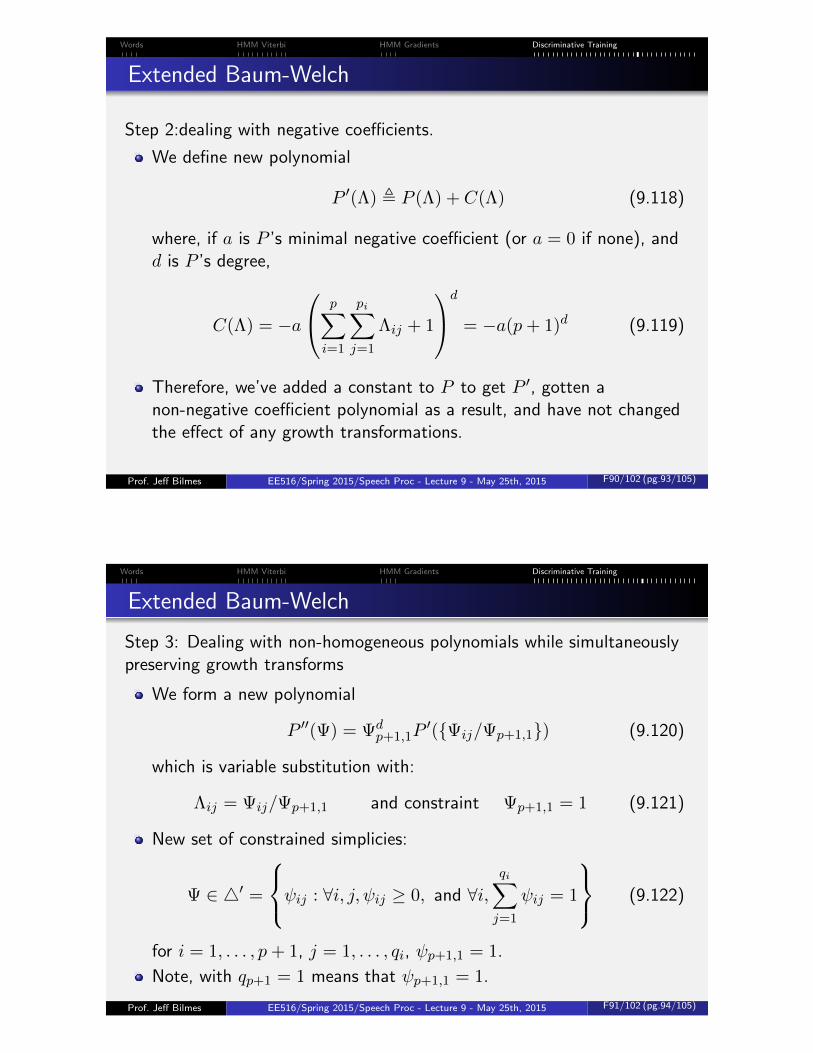
Extended Baum-Welch
Step 2:dealing with negative coefficients.
We define new polynomial
P ′(Λ) , P (Λ) + C(Λ) (9.118)
where, if a is P ’s minimal negative coefficient (or a = 0 if none), andd is P ’s degree,
C(Λ) = −a
p∑i=1
pi∑j=1
Λij + 1
d
= −a(p+ 1)d (9.119)
Therefore, we’ve added a constant to P to get P ′, gotten anon-negative coefficient polynomial as a result, and have not changedthe effect of any growth transformations.
Prof. Jeff Bilmes EE516/Spring 2015/Speech Proc - Lecture 9 - May 25th, 2015 F90/102 (pg.93/105)
Words HMM Viterbi HMM Gradients Discriminative Training
Extended Baum-Welch
Step 3: Dealing with non-homogeneous polynomials while simultaneouslypreserving growth transforms
We form a new polynomial
P ′′(Ψ) = Ψdp+1,1P
′({Ψij/Ψp+1,1}) (9.120)
which is variable substitution with:
Λij = Ψij/Ψp+1,1 and constraint Ψp+1,1 = 1 (9.121)
New set of constrained simplicies:
Ψ ∈ 4′ =
ψij : ∀i, j, ψij ≥ 0, and ∀i,qi∑j=1
ψij = 1
(9.122)
for i = 1, . . . , p+ 1, j = 1, . . . , qi, ψp+1,1 = 1.
Note, with qp+1 = 1 means that ψp+1,1 = 1.
Prof. Jeff Bilmes EE516/Spring 2015/Speech Proc - Lecture 9 - May 25th, 2015 F91/102 (pg.94/105)
Words HMM Viterbi HMM Gradients Discriminative Training
Extended Baum-Welch
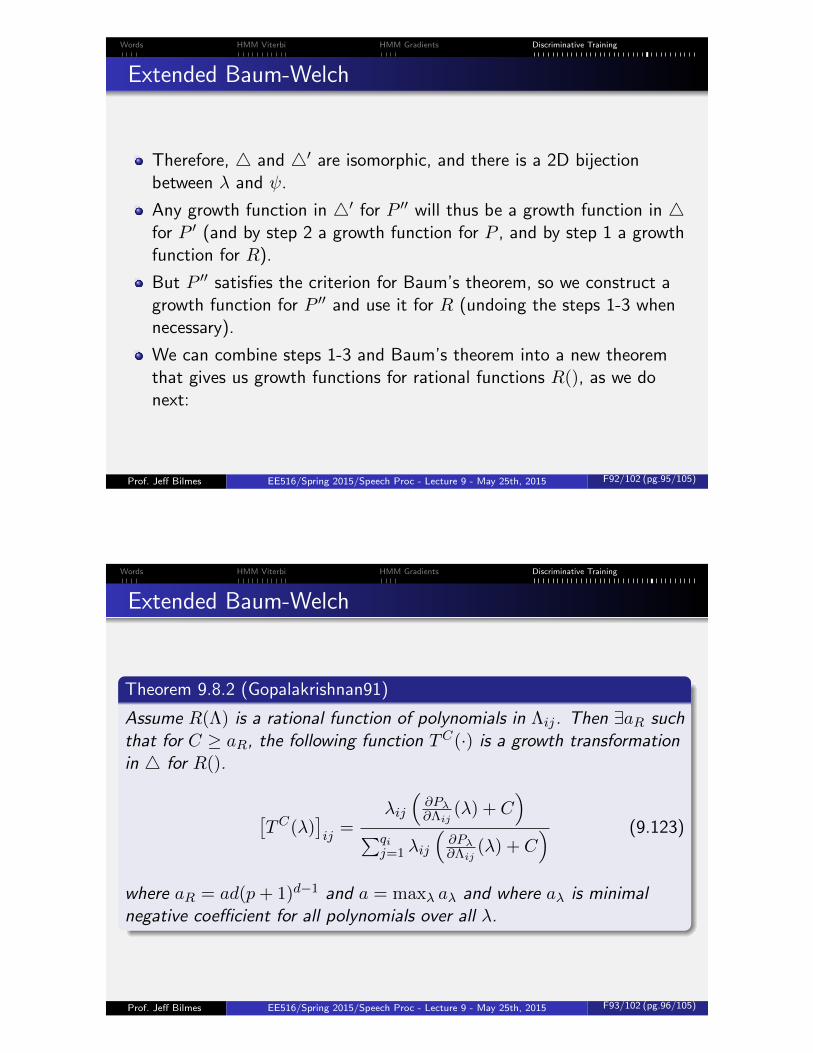
Therefore, 4 and 4′ are isomorphic, and there is a 2D bijectionbetween λ and ψ.
Any growth function in 4′ for P ′′ will thus be a growth function in 4for P ′ (and by step 2 a growth function for P , and by step 1 a growthfunction for R).
But P ′′ satisfies the criterion for Baum’s theorem, so we construct agrowth function for P ′′ and use it for R (undoing the steps 1-3 whennecessary).
We can combine steps 1-3 and Baum’s theorem into a new theoremthat gives us growth functions for rational functions R(), as we donext:
Prof. Jeff Bilmes EE516/Spring 2015/Speech Proc - Lecture 9 - May 25th, 2015 F92/102 (pg.95/105)
Words HMM Viterbi HMM Gradients Discriminative Training
Extended Baum-Welch
Theorem 9.8.2 (Gopalakrishnan91)
Assume R(Λ) is a rational function of polynomials in Λij . Then ∃aR suchthat for C ≥ aR, the following function TC(·) is a growth transformationin 4 for R().
[TC(λ)
]ij
=λij
(∂Pλ∂Λij
(λ) + C)
∑qij=1 λij
(∂Pλ∂Λij
(λ) + C) (9.123)
where aR = ad(p+ 1)d−1 and a = maxλ aλ and where aλ is minimalnegative coefficient for all polynomials over all λ.
Prof. Jeff Bilmes EE516/Spring 2015/Speech Proc - Lecture 9 - May 25th, 2015 F93/102 (pg.96/105)

Words HMM Viterbi HMM Gradients Discriminative Training
MMIE training and growth transformations
We can apply this to MMIE training, where in this case we get (foruniform word priors)
Zλ = 2Iλ(q;x) =pλ(x|q)pλ(x)
=pλ(x|q)∑q′ pλ(x|q′) (9.124)
In discrete case we get update equations:
at+1ij =
atij
(∂logZλ∂aij
(λ) + C(λ))
∑qij=1 a
tij
(∂logZλ∂aij
(λ) + C(λ)) (9.125)
and similar for the other HMM parameters.
Prof. Jeff Bilmes EE516/Spring 2015/Speech Proc - Lecture 9 - May 25th, 2015 F94/102 (pg.97/105)
Words HMM Viterbi HMM Gradients Discriminative Training
Extended Baum-Welch
Note, that we have lower bound on C.
We can prove convergence if C is large enough, but as C gets larger,convergence takes a long time - tradeoff
Heuristic: choose least possible value and double it.
Prof. Jeff Bilmes EE516/Spring 2015/Speech Proc - Lecture 9 - May 25th, 2015 F95/102 (pg.98/105)

Words HMM Viterbi HMM Gradients Discriminative Training
Generative vs. Discriminative Modeling of Data
z
Prof. Jeff Bilmes EE516/Spring 2015/Speech Proc - Lecture 9 - May 25th, 2015 F96/102 (pg.99/105)
Words HMM Viterbi HMM Gradients Discriminative Training
Other forms of discriminative training
Is posterior probability p(q|x) most important thing to optimize?
Bayes Decision Theory says minimum error from:
q∗(x) ∈ argmaxq
p(q|x) (9.126)
But to get q∗(x), we don’t need all the information that exists in theposterior distribution p(q|x), rather we need only the maximum value.Hence, we can approximate the posterior (ask for less information)without error.
Ex. approximations to the posterior (for small random ε):
q∗(x) ∈ argmaxq
(p(q|x) + ε) (9.127)
Since goal is only q∗(x), why not train a model using objective thatmeasures performance based only on q∗(x), and on full posterior?
Rather than ask for something that is more than what we need (theposterior). Need only find discriminant function that gets low error.
Prof. Jeff Bilmes EE516/Spring 2015/Speech Proc - Lecture 9 - May 25th, 2015 F97/102 (pg.100/105)

Words HMM Viterbi HMM Gradients Discriminative Training
Error training
This is related to risk minimization with an error-based loss function,but here done for speech.
With discriminant function gq, we could produce decision rule:
q∗(x) = argmaxq
gq(x|λ) (9.128)
Prof. Jeff Bilmes EE516/Spring 2015/Speech Proc - Lecture 9 - May 25th, 2015 F98/102 (pg.101/105)
Words HMM Viterbi HMM Gradients Discriminative Training
MCE training
Minimum classification error (MCE) training, in speech recognition,has the goal to minimize classification error function directly.
Approach: Error function is a discrete “counting” function,non-differential, hard to optimize continuous parameter space usingthis objective.
Instead, use “smooth” continuous differentiable approximations tofunctions like “max”, and “sign” with smoothness parameters that inthe limit approach the hard versions.
Example:
maxigi = lim
η→∞log
1
N
∑j
exp(gjη)
1/η
(9.129)
For reasonable sized η, this is a “nice” function.
Prof. Jeff Bilmes EE516/Spring 2015/Speech Proc - Lecture 9 - May 25th, 2015 F99/102 (pg.102/105)

Words HMM Viterbi HMM Gradients Discriminative Training
MCE training
Uses these smoothing functions to approximate classification error,and then use gradient descent to train.
Misclassification measure:
di(X) = −gi(X|Λ) + log
1
N − 1
∑j 6=i
exp(gi(X|Λ)η)
1/η
(9.130)
For large enough η, if this is di(X) > 0, then misclassification occurswhen we decide class i.
Loss function (measures amount of misclassification):
`(d) =1
1 + exp(−γd+ θ), γ ≥ 1 (9.131)
If d is smaller than zero, no loss occurs, but positive d incurs a loss.
Prof. Jeff Bilmes EE516/Spring 2015/Speech Proc - Lecture 9 - May 25th, 2015 F100/102 (pg.103/105)
Words HMM Viterbi HMM Gradients Discriminative Training
MCE TrainingFinal classification performance criterion (for a X of class i):
`(X|Λ) =M∑i=1
`i(X|Λ)1(X ∈ Ci) (9.132)
over training set:
L(Λ) = Ex{`(X|Λ)} (9.133)
This can be trained using gradient descent.Smoothness parameters are η and λ but tradeoff exists:
high-values means good approximation to true discrete error measure,but higher order Taylor terms are significant which means training willnot be as good.Low-values means smooth functions without significant higher-orderterms, but poor approximation to true discrete error function.
Generalized probabilistic descent (GPD): given smoothness guarantees(bounded functions of Hessian), we have convergence guarantees ofthis algorithm.
Prof. Jeff Bilmes EE516/Spring 2015/Speech Proc - Lecture 9 - May 25th, 2015 F101/102 (pg.104/105)

Words HMM Viterbi HMM Gradients Discriminative Training
Discriminative training and computation
Given training data of D utterances, D ={
(x(i)1:Ti
, w(i))}Di=1
.
ML training requires computing things like:
log∑
q1:T∈Q1:T (w(i)1:Ni
)
p(x(i)1:Ti
, q1:T |λ) (9.134)
for the numerator (i.e., sum over all paths corresponding to worsesequence). This is hard but doable.
Discriminative training requires computing a denominator, which issomething of the form:
log∑w1:N
∑q1:T∈Q1:T (w1:N )
p(x(i)1:Ti
, q1:T |λ) = log p(x(i)1:Ti|λ) (9.135)
This is computationally intractable, and hence we need a way ofapproximating the denominator.
Prof. Jeff Bilmes EE516/Spring 2015/Speech Proc - Lecture 9 - May 25th, 2015 F102/102 (pg.105/105)


![Chapter 14 Text and Phonetic Analysis Young-ah Do [ Spoken Language Processing ] Xuedong Huang, Alex Acero, Hsiao-Wuen Hon.](https://static.fdocuments.us/doc/165x107/5697bf8f1a28abf838c8d297/chapter-14-text-and-phonetic-analysis-young-ah-do-spoken-language-processing.jpg)