EE382C Lecture 5 - Stanford University
31
EE 382C - S11 - Lecture 5 1 EE382C Lecture 5 Introduction to Routing 4/12/11
Transcript of EE382C Lecture 5 - Stanford University
EE 382C - S11 - Lecture 5
1
EE382C
Lecture 5
Introduction to Routing
4/12/11
EE 382C - S11 - Lecture 5
2
Logistics
• Homework 1 due NOW
• Homework 2: 8.1, 8.9, 9.5, 10.4
EE 382C - S11 - Lecture 5
3
Question of the day
What oblivious routing algorithm should you use on a 8-ary 2-
cube to maximize worst-case throughput?
What does this algorithm do to the latency of nearest-neighbor
traffic?
Can you optimize both at the same time?
EE 382C - S11 - Lecture 5
4
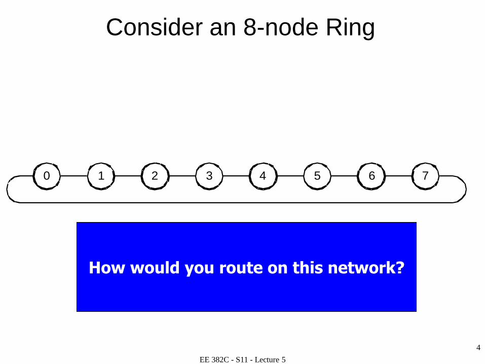
Consider an 8-node Ring
1 2 3 4 5 6 70
How would you route on this network?
EE 382C - S11 - Lecture 5
5
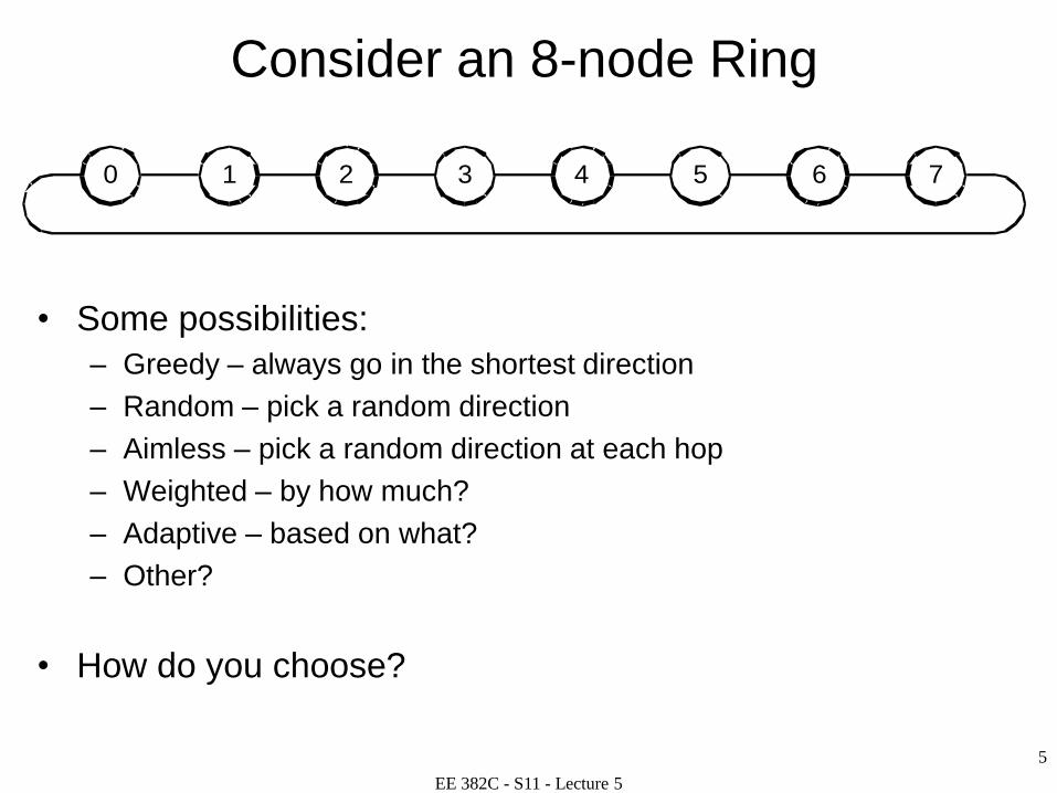
Consider an 8-node Ring
• Some possibilities:
– Greedy – always go in the shortest direction
– Random – pick a random direction
– Aimless – pick a random direction at each hop
– Weighted – by how much?
– Adaptive – based on what?
– Other?
• How do you choose?
1 2 3 4 5 6 70
EE 382C - S11 - Lecture 5
6
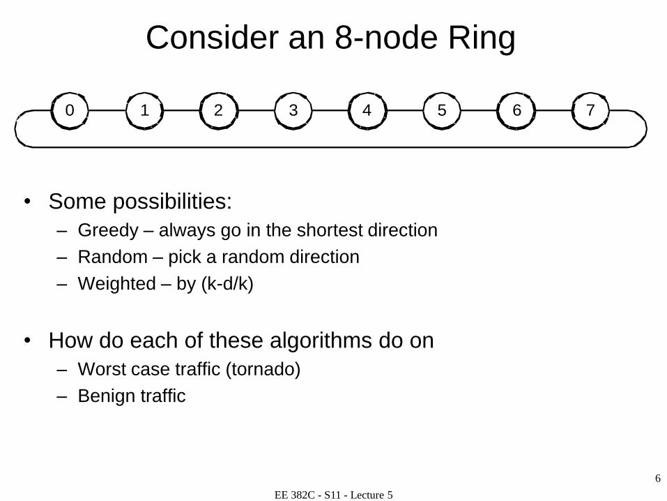
Consider an 8-node Ring
• Some possibilities:
– Greedy – always go in the shortest direction
– Random – pick a random direction
– Weighted – by (k-d/k)
• How do each of these algorithms do on
– Worst case traffic (tornado)
– Benign traffic
1 2 3 4 5 6 70
EE 382C - S11 - Lecture 5
7
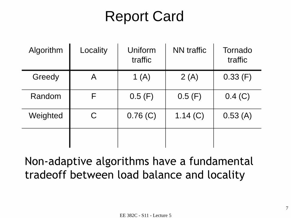
Report Card
Algorithm Locality Uniform
traffic
NN traffic Tornado
traffic
Greedy A 1 (A) 2 (A) 0.33 (F)
Random F 0.5 (F) 0.5 (F) 0.4 (C)
Weighted C 0.76 (C) 1.14 (C) 0.53 (A)
Non-adaptive algorithms have a fundamental
tradeoff between load balance and locality
EE 382C - S11 - Lecture 5
8
Routing basics (1)
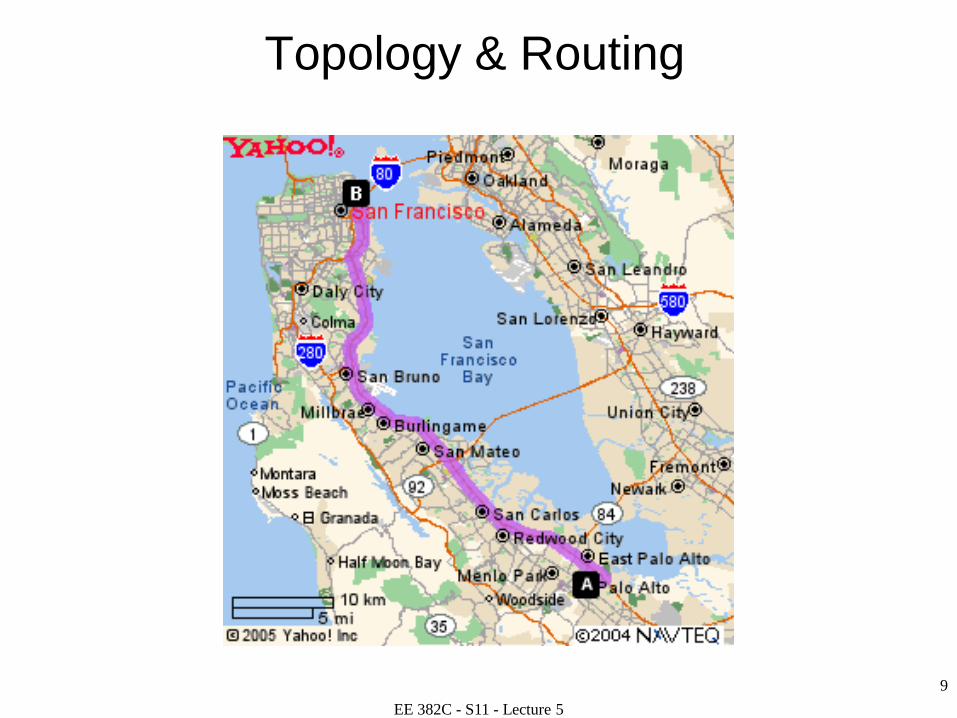
• Topology sets a “roadmap” between nodes
– Specific topology chosen to exploit packaging technology, meet
application requirements (bandwidth, latency, scalability, etc.) at the
minimum cost
• Topology fixes performance bounds
– Efficient routing (& flow control) strives to achieve these bounds
• Routing determines how data navigates through this
roadmap
– Determines a path (ordered set of channels) from source to
destination
EE 382C - S11 - Lecture 5
9
Topology & Routing
EE 382C - S11 - Lecture 5
10
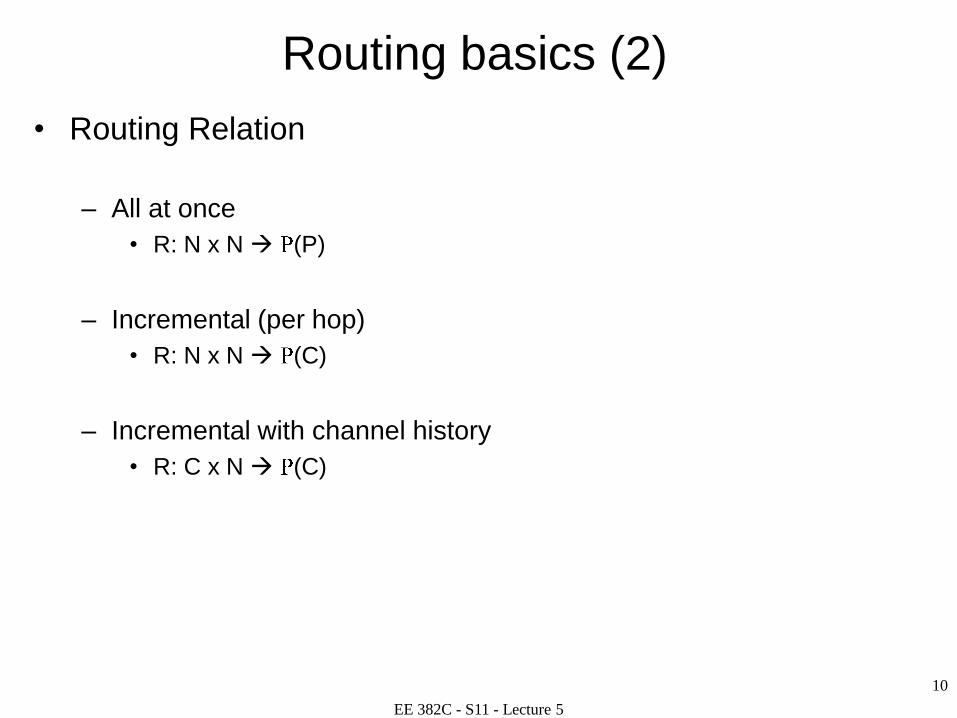
Routing basics (2)
• Routing Relation
– All at once
• R: N x N (P)
– Incremental (per hop)
• R: N x N (C)
– Incremental with channel history
• R: C x N (C)
EE 382C - S11 - Lecture 5
11
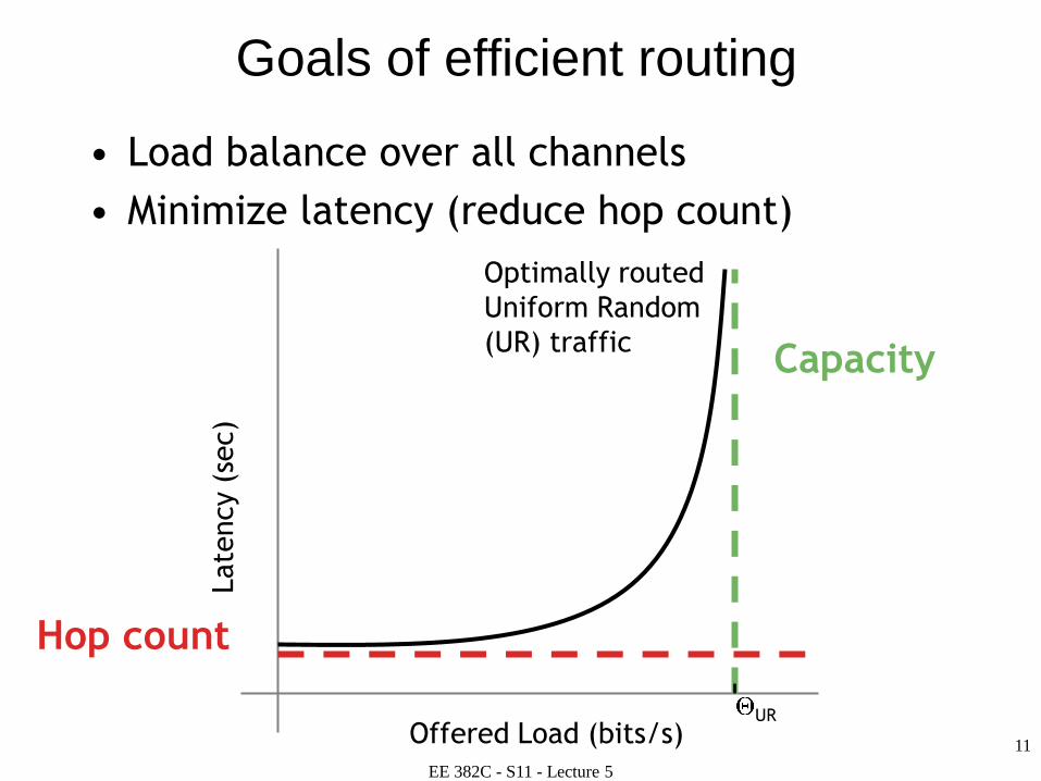
Goals of efficient routing
Capacity
Late
ncy (
sec)
Offered Load (bits/s)
Hop count
UR
Optimally routed
Uniform Random
(UR) traffic
• Load balance over all channels
• Minimize latency (reduce hop count)
EE 382C - S11 - Lecture 5
12
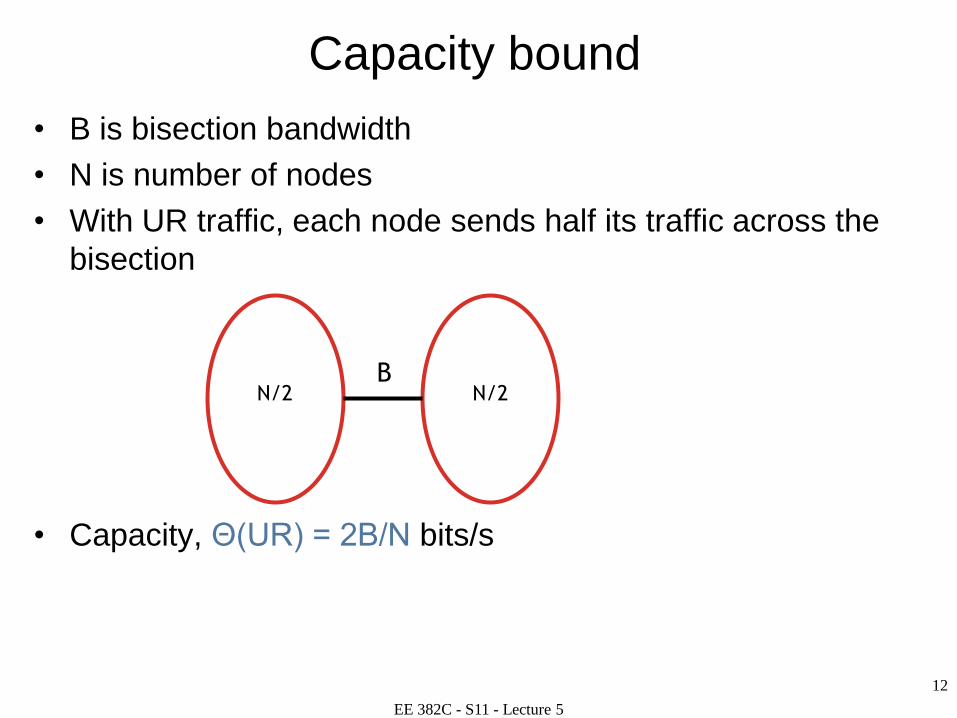
Capacity bound
• B is bisection bandwidth
• N is number of nodes
• With UR traffic, each node sends half its traffic across the
bisection
• Capacity, Θ(UR) = 2B/N bits/s
N/2 N/2B
EE 382C - S11 - Lecture 5
13
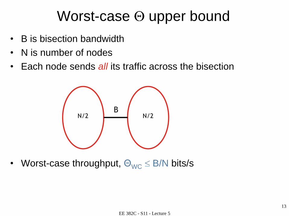
Worst-case upper bound
• B is bisection bandwidth
• N is number of nodes
• Each node sends all its traffic across the bisection
• Worst-case throughput, ΘWC B/N bits/s
N/2 N/2B
EE 382C - S11 - Lecture 5
14
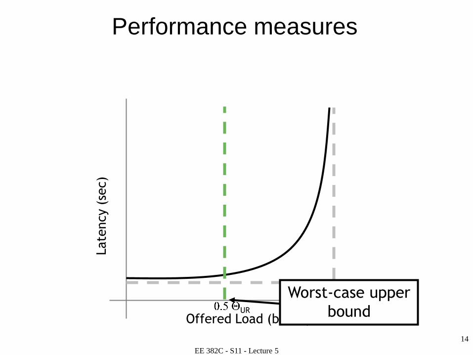
Performance measures
Late
ncy (
sec)
Offered Load (bits/s)URUR
Worst-case upper
bound
EE 382C - S11 - Lecture 5
15
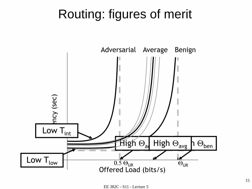
Routing: figures of merit
Late
ncy (
sec)
Offered Load (bits/s)URUR
Benign
High ben
Adversarial
High adv
Average
High avg
Low Tlow
Low Tint
EE 382C - S11 - Lecture 5
16
Taxonomy of routing algos
• Deterministic
– Fixed path from source to destination
• Oblivious
– Can use randomization to select between different paths
• Adaptive
– Can use network state to make routing decisions
EE 382C - S11 - Lecture 5
17
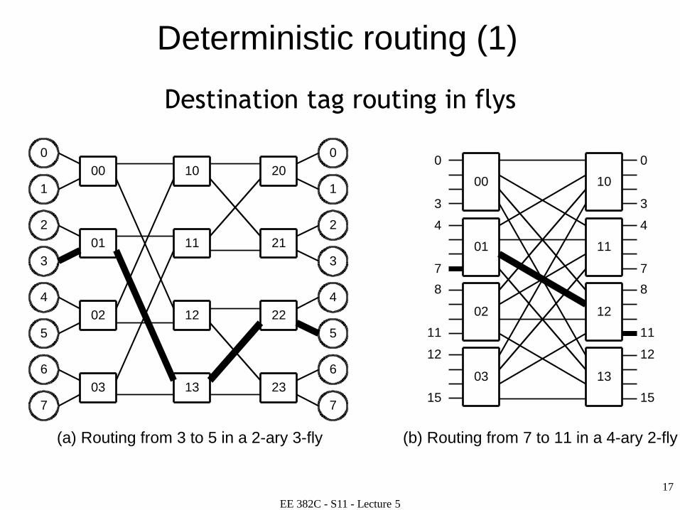
Deterministic routing (1)
0
1
2
3
4
5
6
7
00
01
02
03
10
11
12
13
20
21
22
23
0
1
2
3
4
5
6
7
(a) Routing from 3 to 5 in a 2-ary 3-fly
00
01
02
03
10
11
12
13
0
3
4
7
8
11
12
15
0
3
4
7
8
11
12
15
(b) Routing from 7 to 11 in a 4-ary 2-fly
Destination tag routing in flys
EE 382C - S11 - Lecture 5
18
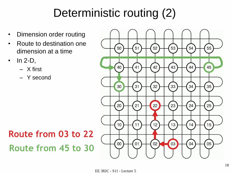
Deterministic routing (2)
• Dimension order routing
• Route to destination one
dimension at a time
• In 2-D,
– X first
– Y second
Route from 03 to 22
Route from 45 to 30
EE 382C - S11 - Lecture 5
19
Oblivious routing
• Path from source A to destination B chosen using
randomization
• Advantages
– Simple analysis and implementation
– Can provide good load balancing
• Disadvantages
– Cannot have both low latency and good load balancing
– Packet reordering
EE 382C - S11 - Lecture 5
20
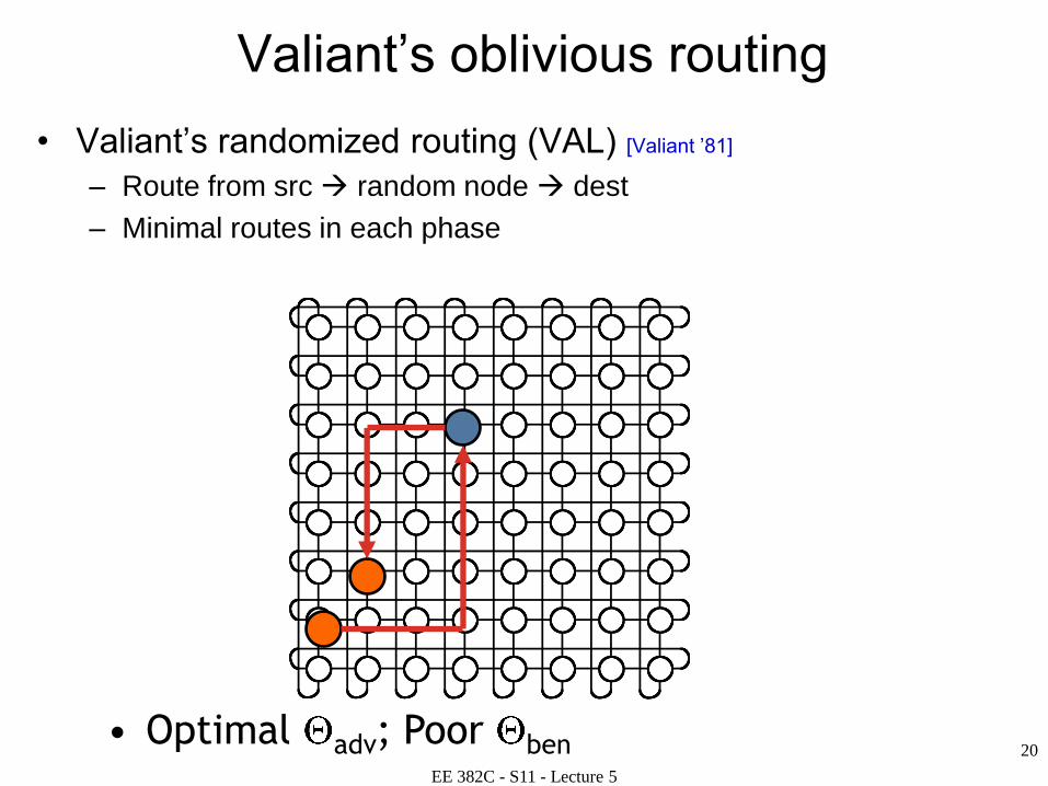
Valiant’s oblivious routing
• Valiant’s randomized routing (VAL) [Valiant ’81]
– Route from src random node dest
– Minimal routes in each phase
• Optimal adv; Poor ben
EE 382C - S11 - Lecture 5
21
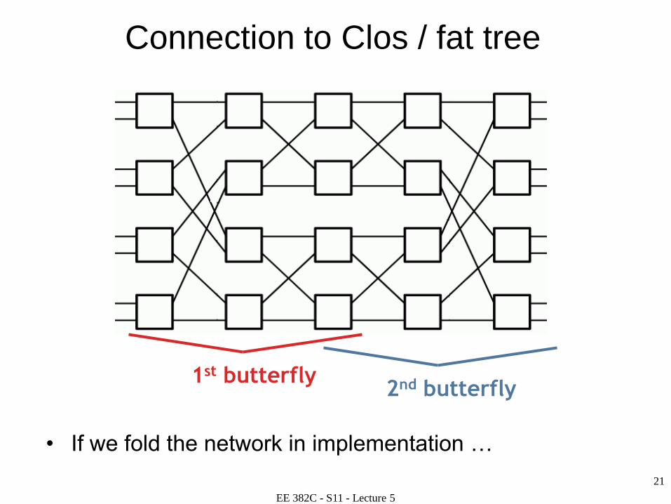
Connection to Clos / fat tree
1st butterfly2nd butterfly
• If we fold the network in implementation …
EE 382C - S11 - Lecture 5
22
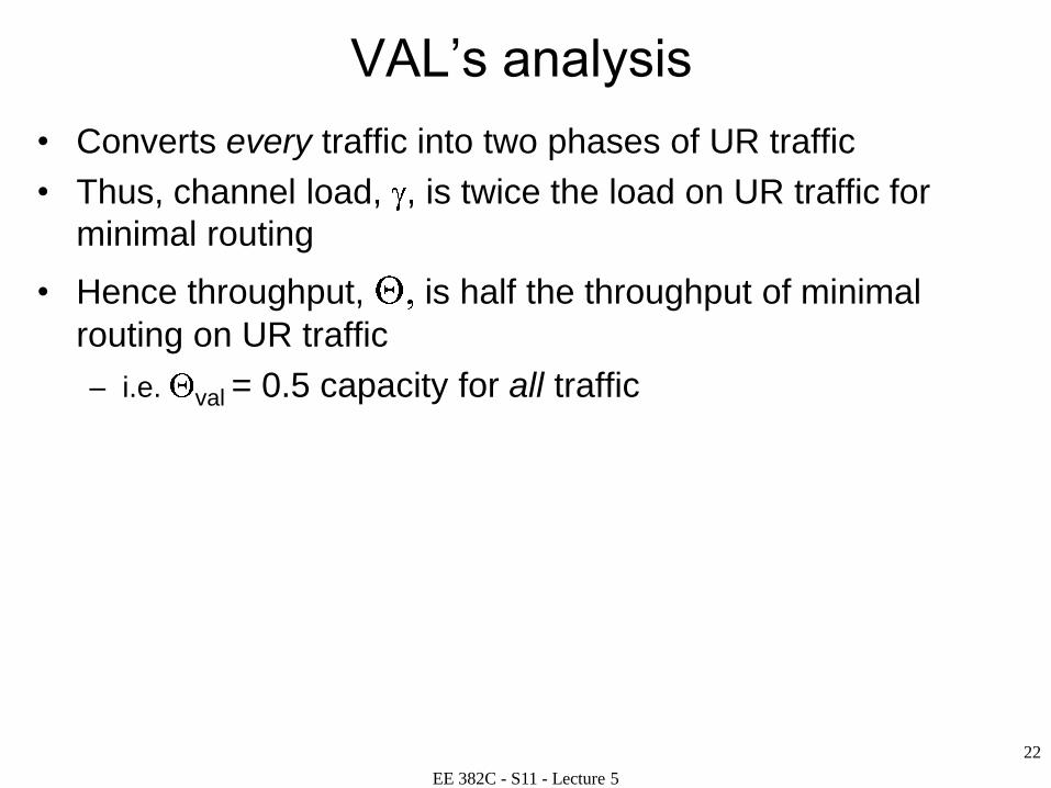
VAL’s analysis
• Converts every traffic into two phases of UR traffic
• Thus, channel load, , is twice the load on UR traffic for
minimal routing
• Hence throughput, is half the throughput of minimal
routing on UR traffic
– i.e. val = 0.5 capacity for all traffic
EE 382C - S11 - Lecture 5
23
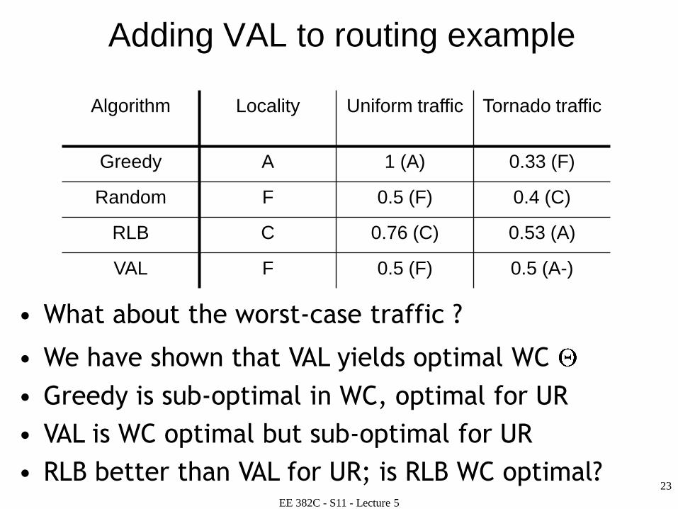
Adding VAL to routing example
Algorithm Locality Uniform traffic Tornado traffic
Greedy A 1 (A) 0.33 (F)
Random F 0.5 (F) 0.4 (C)
RLB C 0.76 (C) 0.53 (A)
VAL F 0.5 (F) 0.5 (A-)
• What about the worst-case traffic ?
• We have shown that VAL yields optimal WC
• Greedy is sub-optimal in WC, optimal for UR
• VAL is WC optimal but sub-optimal for UR
• RLB better than VAL for UR; is RLB WC optimal?
EE 382C - S11 - Lecture 5
24
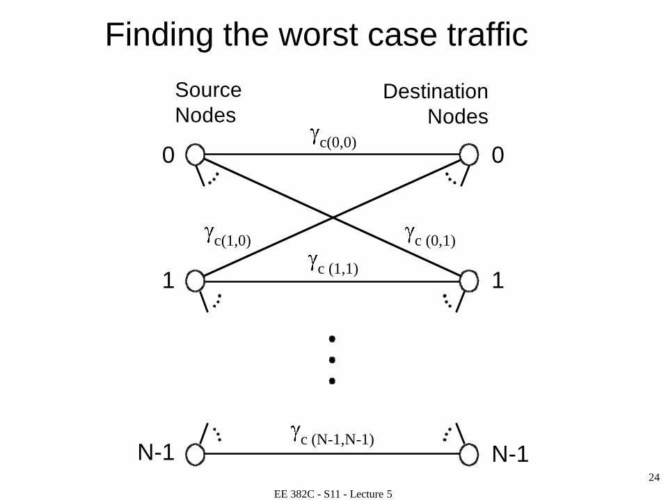
c(0,0)
c (1,1)
c (N-1,N-1)
c (0,1)c(1,0)
0
1
N-1
0
1
N-1
Source
NodesDestination
Nodes
Finding the worst case traffic
EE 382C - S11 - Lecture 5
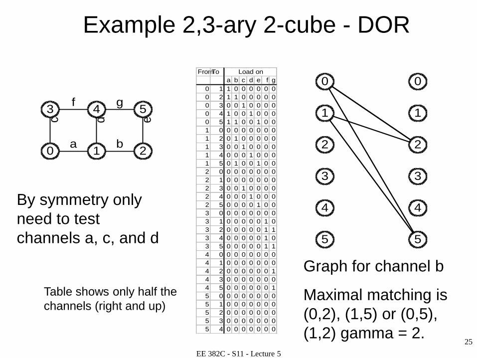
25
Example 2,3-ary 2-cube - DORc d e
gf
ba
3
0
4
1
5
2
By symmetry only
need to test
channels a, c, and d
FromTo
a b c d e f g
0 1 1 0 0 0 0 0 0
0 2 1 1 0 0 0 0 0
0 3 0 0 1 0 0 0 0
0 4 1 0 0 1 0 0 0
0 5 1 1 0 0 1 0 0
1 0 0 0 0 0 0 0 0
1 2 0 1 0 0 0 0 0
1 3 0 0 1 0 0 0 0
1 4 0 0 0 1 0 0 0
1 5 0 1 0 0 1 0 0
2 0 0 0 0 0 0 0 0
2 1 0 0 0 0 0 0 0
2 3 0 0 1 0 0 0 0
2 4 0 0 0 1 0 0 0
2 5 0 0 0 0 1 0 0
3 0 0 0 0 0 0 0 0
3 1 0 0 0 0 0 1 0
3 2 0 0 0 0 0 1 1
3 4 0 0 0 0 0 1 0
3 5 0 0 0 0 0 1 1
4 0 0 0 0 0 0 0 0
4 1 0 0 0 0 0 0 0
4 2 0 0 0 0 0 0 1
4 3 0 0 0 0 0 0 0
4 5 0 0 0 0 0 0 1
5 0 0 0 0 0 0 0 0
5 1 0 0 0 0 0 0 0
5 2 0 0 0 0 0 0 0
5 3 0 0 0 0 0 0 0
5 4 0 0 0 0 0 0 0
Load on
0
1
2
3
4
5
0
1
2
3
4
5
Table shows only half the
channels (right and up)
Graph for channel b
Maximal matching is
(0,2), (1,5) or (0,5),
(1,2) gamma = 2.
EE 382C - S11 - Lecture 5
26
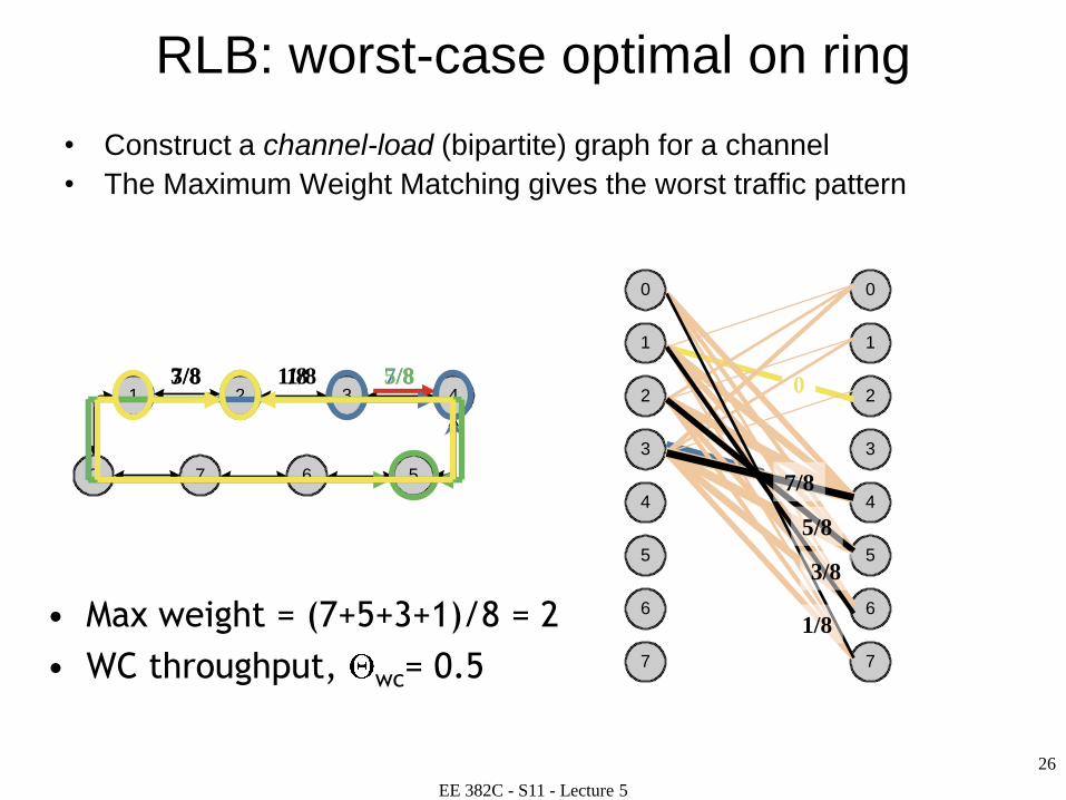
RLB: worst-case optimal on ring
• Construct a channel-load (bipartite) graph for a channel
• The Maximum Weight Matching gives the worst traffic pattern
1 2 3 4
5670
0 0
2 2
3 3
5 5
6 6
1 1
4 4
7 7
7/81/8
7/8
5/83/8
5/8
7/8 1/8 0
• Max weight = (7+5+3+1)/8 = 2
• WC throughput, wc= 0.5
1/8
3/8
5/8
7/8
EE 382C - S11 - Lecture 5
27
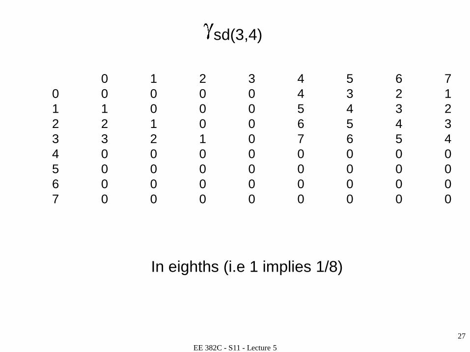
sd(3,4)
0 1 2 3 4 5 6 7
0 0 0 0 0 4 3 2 1
1 1 0 0 0 5 4 3 2
2 2 1 0 0 6 5 4 3
3 3 2 1 0 7 6 5 4
4 0 0 0 0 0 0 0 0
5 0 0 0 0 0 0 0 0
6 0 0 0 0 0 0 0 0
7 0 0 0 0 0 0 0 0
In eighths (i.e 1 implies 1/8)
EE 382C - S11 - Lecture 5
28
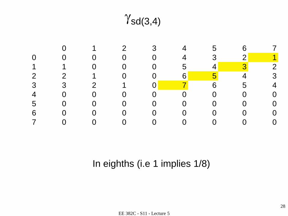
sd(3,4)
0 1 2 3 4 5 6 7
0 0 0 0 0 4 3 2 1
1 1 0 0 0 5 4 3 2
2 2 1 0 0 6 5 4 3
3 3 2 1 0 7 6 5 4
4 0 0 0 0 0 0 0 0
5 0 0 0 0 0 0 0 0
6 0 0 0 0 0 0 0 0
7 0 0 0 0 0 0 0 0
In eighths (i.e 1 implies 1/8)
EE 382C - S11 - Lecture 5
29
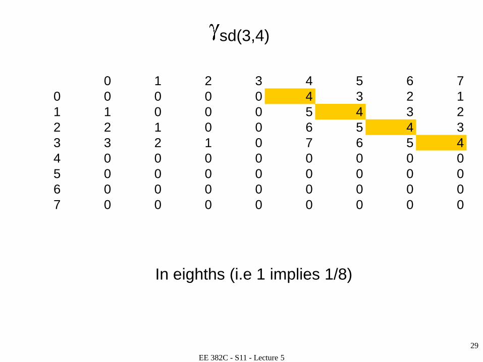
sd(3,4)
0 1 2 3 4 5 6 7
0 0 0 0 0 4 3 2 1
1 1 0 0 0 5 4 3 2
2 2 1 0 0 6 5 4 3
3 3 2 1 0 7 6 5 4
4 0 0 0 0 0 0 0 0
5 0 0 0 0 0 0 0 0
6 0 0 0 0 0 0 0 0
7 0 0 0 0 0 0 0 0
In eighths (i.e 1 implies 1/8)
EE 382C - S11 - Lecture 5
30
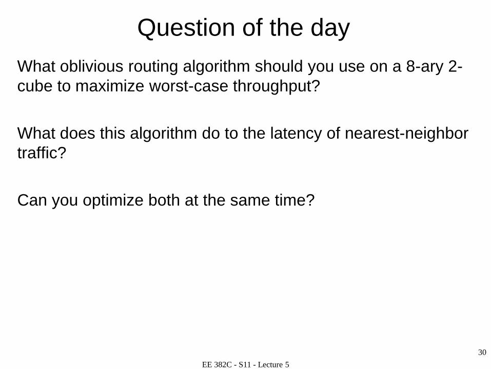
Question of the day
What oblivious routing algorithm should you use on a 8-ary 2-
cube to maximize worst-case throughput?
What does this algorithm do to the latency of nearest-neighbor
traffic?
Can you optimize both at the same time?
EE 382C - S11 - Lecture 5
31
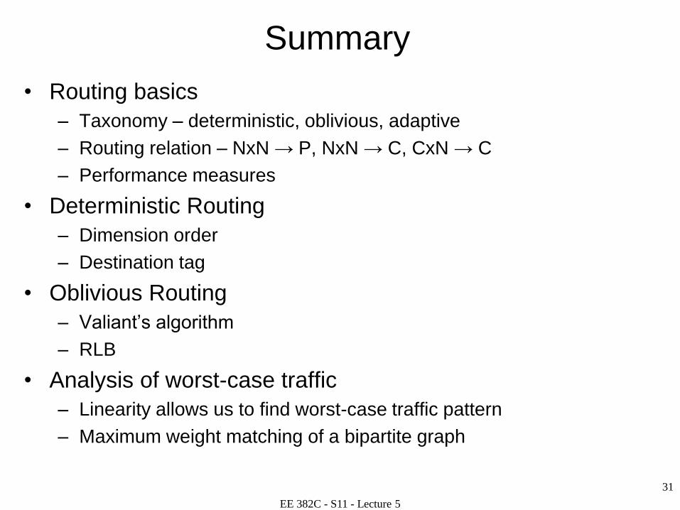
Summary
• Routing basics
– Taxonomy – deterministic, oblivious, adaptive
– Routing relation – NxN → P, NxN → C, CxN → C
– Performance measures
• Deterministic Routing
– Dimension order
– Destination tag
• Oblivious Routing
– Valiant’s algorithm
– RLB
• Analysis of worst-case traffic
– Linearity allows us to find worst-case traffic pattern
– Maximum weight matching of a bipartite graph