EE123 Digital Signal Processing - EECS Instructional ...ee123/sp15/Notes/Lecture06_DFT... · Linear...
30
M. Lustig, EECS UC Berkeley EE123 Digital Signal Processing Lecture 6 Properties of DFT based on slides by J.M. Kahn
-
Upload
phungthuan -
Category
Documents
-
view
221 -
download
0
Transcript of EE123 Digital Signal Processing - EECS Instructional ...ee123/sp15/Notes/Lecture06_DFT... · Linear...

M. Lustig, EECS UC Berkeley
EE123Digital Signal Processing
Lecture 6Properties of DFT
based on slides by J.M. Kahn
M. Lustig, EECS UC Berkeley
Announcements
• HW1 solutions posted -- self grading due• HW2 due Friday
• SDR give after GSI Wednesday• Finish reading Ch. 8, start Ch. 9
• ham radio licensing lectures Tue 6:30-8pm Cory 521

M. Lustig, EECS UC Berkeley
Cool things DSP
• Cosmic MicrowaveBackground radiation

M. Lustig, EECS UC Berkeley
Last Time
• Discrete Fourier Transform– Similar to DFS– Sampling of the DTFT (subtitles....more later)– Properties of the DFT
• Today– Linear convolution with DFT– Fast Fourier Transform

x[((n�m))N ] $ X[k]e�j(2⇡/N)km = X[k]W kmN
M. Lustig, EECS UC Berkeley
Properties of DFT
• Inherited from DFS (EE120/20) so no need to be proved
• Linearity
• Circular Time Shift
↵1x1[n] + ↵2x2[n] $ ↵1X1[k] + ↵2X2[k]
M. Lustig, EECS UC Berkeley
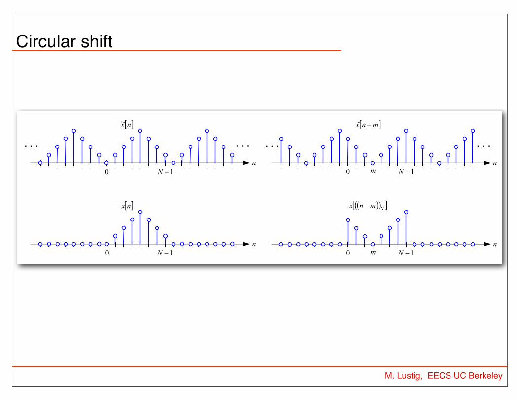
Circular shift
! "mnx #~
n
0 1#N
. . . . . .
m
$ %$ %! "N
mnx #
n
0 1#Nm
! "nx~
n
0 1#N
. . . . . .
! "nx
n
0 1#N

M. Lustig, EECS UC Berkeley
Properties of DFT
• Circular frequency shift
• Complex Conjugation
• Conjugate Symmetry for Real Signals
x[n]ej(2⇡/N)nl = x[n]W�nlN $ X[((k � l))N ]
x
⇤[n] $ X
⇤[((�k))N ]
x[n] = x
⇤[n] $ X[k] = X
⇤[((�k))N ]
Show....

M. Lustig, EECS UC Berkeley
Properties of DFT
• Parseval’s Identity
• Proof (in matrix notation)
N�1X
n=0
|x[n]|2 =1
N
N�1X
k=0
|X[k]|2
x
⇤x =
✓1
NW
⇤NX
◆⇤ ✓ 1
NW
⇤NX
◆=
1
N2X
⇤WNW
⇤N| {z }
N ·I
X =1
NX
⇤X

M. Lustig, EECS UC Berkeley
Circular Convolution Sum
• Circular Convolution:
for two signals of length N
x1[n]�N x2[n]�=
N�1X
m=0
x1[m]x2[((n�m))N ]
x2[n]�N x1[n] = x1[n]�N x2[n]
• Note: Circular convolution is commutative
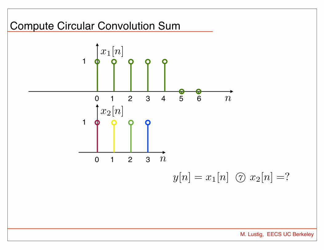
x1[n]
x2[n]
y[n] = x1[n] �7 x2[n] =?
M. Lustig, EECS UC Berkeley
Compute Circular Convolution Sum
n0 1 2 3 4
1
n0 1 2
1
5 6
3

x1[n]
x2[n]
M. Lustig, EECS UC Berkeley
Compute Circular Convolution Sum
n0 1 2 3 4
1
n0 1 2
1
5 6
3 4 5 6
Circular ‘flip’multiply and addHere: y[0]
y[n] = x1[n] �7 x2[n] =?
x1[n]
x2[n]
M. Lustig, EECS UC Berkeley
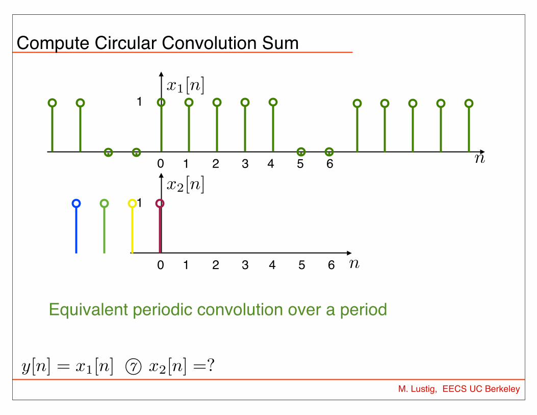
Compute Circular Convolution Sum
n0 1 2 3 4
1
n0 1 2
1
5 6
3 4 5 6
Equivalent periodic convolution over a period
y[n] = x1[n] �7 x2[n] =?

M. Lustig, EECS UC Berkeley
Result
n0 1 2 3 4
2
5 6
y[n] = x1[n] �7 x2[n] =?4

M. Lustig, EECS UC Berkeley
Properties of DFT
• Circular Convolution: Let x1[n], x2[n] be length N
• Multiplication: Let x1[n], x2[n] be length N
x1[n]�N x2[n] $ X1[k] ·X2[k]
x1[n] · x2[n] $1
N
X1[k]�N X2[k]
Very useful!!! ( for linear convolutions with DFT)

M. Lustig, EECS UC Berkeley
Linear Convolution
• Next....– Using DFT, circular convolution is easy – But, linear convolution is useful, not circular– So, show how to perform linear convolution
with circular convolution – Used DFT to do linear convolution

M. Lustig, EECS UC Berkeley
Linear Convolution
• We start with two non-periodic sequences:
• We want to compute the linear convolution:
• Requires L·P multiplications
for example x[n] is a signal and h[n] an impulse response of a filter
x[n] 0 n L� 1
h[n] 0 n P � 1
y[n] = x[n] ⇤ h[n] =L�1X
m=0
x[m]h[n�m]
y[n] is nonzero for 0 ≤ n ≤ L+P-2 with length M=L+P-1

M. Lustig, EECS UC Berkeley
Linear Convolution via Circular Convolution
• Zero-pad x[n] by P-1 zeros
• Zero-pad h[n] by L-1 zeros
• Now, both sequences are of length M=L+P-1
xzp[n] =
⇢x[n] 0 n L� 10 L n L+ P � 2
hzp[n] =
⇢h[n] 0 n P � 10 P n L+ P � 2

M. Lustig, EECS UC Berkeley
Linear Convolution via Circular Convolution
• Now, both sequences are of length M=L+P-1
• We can now compute the linear convolution using a circular one with length M = L+P-1
Linear Convolution using the DFT
Both zero-padded sequences xzp
[n] and hzp
[n] are of lengthM = L+ P � 1
We can compute the linear convolution x [n] ⇤ h[n] = y [n] bycomputing circular convolution x
zp
[n]�M hzp
[n]:
Linear convolution via circular
y [n] = x [n] ⇤ y [n] =(xzp
[n]�M hzp
[n] 0 n M � 1
0 otherwise
Miki Lustig UCB. Based on Course Notes by J.M Kahn Fall 2012, EE123 Digital Signal Processing

x1[n]
x2[n]
M. Lustig, EECS UC Berkeley
Example
n0 1 2 3 4
1
n0 1 2
1
3
L=5
P=4
M = L + P - 1 = 8

x1[n]
x2[n]
M. Lustig, EECS UC Berkeley
Example
n0 1 2 3 4
1
n0 1 2
1
3
M = L + P - 1 = 8
6 75
4 6 75

x1[n]
x2[n]
y[n] = x1[n] �8 x2[n] = x1[n] ⇤ x2[n]
M. Lustig, EECS UC Berkeley
Example
n0 1 2 3 4
1
n0 1 2
1
3
M = L + P - 1 = 8
6 75
4 6 75
Circular ‘flip’

M. Lustig, EECS UC Berkeley
Linear Convolution using DFT
• In practice we can implement a circulant convolution using the DFT property:
• Advantage: DFT can be computed with Nlog2N complexity (FFT algorithm later!)
• Drawback: Must wait for all the samples -- huge delay -- incompatible with real-time
x[n] ⇤ h[n] = xzp[n]�M hzp[n]
= DFT �1 {DFT {xzp[n]} · DFT {hzp[n]}}for 0 ≤ n ≤ M-1, M=L+P-1

M. Lustig, EECS UC Berkeley
Block Convolution
• Problem: – An input signal x[n], has very long length
(could be considered infinite)– An impulse response h[n] has length P– We want to take advantage of DFT/FFT and
compute convolutions in blocks that are shorter than the signal
• Approach:– Break the signal into small blocks– Compute convolutions– Combine the results

M. Lustig, EECS UC Berkeley
Block Convolution
Example:
0 10 20 30
-0.5
0
0.5
n
x[n]
Input Signal, Length 33
0 10 20 30
-0.5
0
0.5
n
h[n]
Impulse Response, Length P = 6
0 10 20 30
-0.5
0
0.5
n
y[n]
Linear Convolution, Length 38
Miki Lustig UCB. Based on Course Notes by J.M Kahn Fall 2012, EE123 Digital Signal Processing
Block Convolution
Example:
0 10 20 30
-0.5
0
0.5
n
x[n]
Input Signal, Length 33
0 10 20 30
-0.5
0
0.5
n
h[n]
Impulse Response, Length P = 6
0 10 20 30
-0.5
0
0.5
n
y[n]
Linear Convolution, Length 38
Miki Lustig UCB. Based on Course Notes by J.M Kahn Fall 2012, EE123 Digital Signal Processing
Block Convolution
Example:
0 10 20 30
-0.5
0
0.5
n
x[n]
Input Signal, Length 33
0 10 20 30
-0.5
0
0.5
n
h[n]
Impulse Response, Length P = 6
0 10 20 30
-0.5
0
0.5
n
y[n]
Linear Convolution, Length 38
Miki Lustig UCB. Based on Course Notes by J.M Kahn Fall 2012, EE123 Digital Signal Processing
h[n] Impulse response, Length P=6
x[n] Input Signal, Length P=33 y[n] Output Signal, Length P=38
Block Convolution
Example:

Overlap-Add Method
We decompose the input signal x [n] into non-overlapping segmentsxr
[n] of length L:
xr
[n] =
(x [n] rL n (r + 1)L� 1
0 otherwise
The input signal is the sum of these input segments:
x [n] =1X
r=0
xr
[n]
The output signal is the sum of the output segments xr
[n] ⇤ h[n]:
y [n] = x [n] ⇤ h[n] =1X
r=0
xr
[n] ⇤ h[n] (1)
Each of the output segments xr
[n] ⇤ h[n] is of lengthN = L+ P � 1.Miki Lustig UCB. Based on Course Notes by J.M Kahn Fall 2012, EE123 Digital Signal ProcessingSP 2015

Overlap-Add Method
We can compute each output segment xr
[n] ⇤ h[n] with linearconvolution.DFT-based circular convolution is usually more e�cient:
Zero-pad input segment xr
[n] to obtain xr ,zp[n], of length N.
Zero-pad the impulse response h[n] to obtain hzp
[n], of lengthN (this needs to be done only once).Compute each output segment using:
xr
[n] ⇤ h[n] = DFT �1 {DFT {xr ,zp[n]} · DFT {h
zp
[n]}}
Since output segment xr
[n] ⇤ h[n] starts o↵set from its neighborxr�1
[n] ⇤ h[n] by L, neighboring output segments overlap at P � 1points.Finally, we just add up the output segments using (1) to obtain theoutput.
Miki Lustig UCB. Based on Course Notes by J.M Kahn Fall 2012, EE123 Digital Signal ProcessingSP 2015

Overlap-Add Method
0 10 20 30
-0.5
0
0.5
n
x 0[n]
Overlap-Add, Input Segments, Length L = 11
0 10 20 30
-0.5
0
0.5
n
y 0[n]
Overlap-Add, Output Segments, Length L+P-1 = 16
0 10 20 30
-0.5
0
0.5
n
x 1[n]
0 10 20 30
-0.5
0
0.5
n
y 1[n]
0 10 20 30
-0.5
0
0.5
n
x 2[n]
0 10 20 30
-0.5
0
0.5
n
y 2[n]
0 10 20 30
-0.5
0
0.5
n
x[n]
Overlap-Add, Sum of Input Segments
0 10 20 30
-0.5
0
0.5
n
y[n]
Overlap-Add, Sum of Output Segments
Miki Lustig UCB. Based on Course Notes by J.M Kahn Fall 2012, EE123 Digital Signal Processing
Block Convolution
Example:
0 10 20 30
-0.5
0
0.5
n
x[n]
Input Signal, Length 33
0 10 20 30
-0.5
0
0.5
n
h[n]
Impulse Response, Length P = 6
0 10 20 30
-0.5
0
0.5
n
y[n]
Linear Convolution, Length 38
Miki Lustig UCB. Based on Course Notes by J.M Kahn Fall 2012, EE123 Digital Signal Processing
Block Convolution
Example:
0 10 20 30
-0.5
0
0.5
n
x[n]
Input Signal, Length 33
0 10 20 30
-0.5
0
0.5
n
h[n]
Impulse Response, Length P = 6
0 10 20 30
-0.5
0
0.5
n
y[n]
Linear Convolution, Length 38
Miki Lustig UCB. Based on Course Notes by J.M Kahn Fall 2012, EE123 Digital Signal Processing
x0[n]
x1[n]
x2[n]
x[n] = x0[n]+x1[n]+x2[n] y[n] = y0[n]+y1[n]+y2[n]
x0[n]
x1[n]
x2[n]
Example of overlap and add:

Overlap-Save Method
Basic IdeaWe split the input signal x [n] into overlapping segments x
r
[n] oflength L+ P � 1.Perform a circular convolution of each input segment x
r
[n] withthe impulse response h[n], which is of length P using the DFT.Identify the L-sample portion of each circular convolution thatcorresponds to a linear convolution, and save it.This is illustrated below where we have a block of L samplescircularly convolved with a P sample filter.
Miki Lustig UCB. Based on Course Notes by J.M Kahn Fall 2012, EE123 Digital Signal ProcessingSP 2015

M. Lustig, EECS UC Berkeley
Recall:x1[n]
x2[n]
n0 1 2 3 4
1
n0 1 2
1
5 6
3 4 5 6
n0 1 2 3 4
2
5 6
4Valid linear convolution!

Overlap-Save Method
0 10 20 30
-0.5
0
0.5
n
y[n]
Overlap-Save, Concatenation of Usable Output Segments
0 10 20 30
-0.5
0
0.5
n
x 0[n]
Overlap-Save, Input Segments, Length L = 16
0 10 20 30
-0.5
0
0.5
n
y 0p[n
]
Overlap-Save, Output Segments, Usable Length L - P + 1
Usable (y0[n])
Unusable
0 10 20 30
-0.5
0
0.5
n
x 1[n]
0 10 20 30
-0.5
0
0.5
n
y 1p[n
]
Usable (y1[n])
Unusable
0 10 20 30
-0.5
0
0.5
n
x 2[n)
0 10 20 30
-0.5
0
0.5
n
y 2p[n
]
Usable (y2[n])
Unusable
Miki Lustig UCB. Based on Course Notes by J.M Kahn Fall 2012, EE123 Digital Signal ProcessingSP 2015
Example of overlap and save:


![EE123 Digital Signal Processing - University of …ee123/sp16/Notes/Lecture05_DFT... · EE123 Digital Signal Processing ... (DFT {X ⇤ [k]})⇤ •Implement IDFT by: ... Linear Convolution](https://static.fdocuments.us/doc/165x107/5b7e37597f8b9a03248b9e7c/ee123-digital-signal-processing-university-of-ee123sp16noteslecture05dft.jpg)