EDUSAT LEARNING RESOURCE MATERIAL ON › wp-content › plugins › LectureNote › uploa… ·...
54
Copy Right DTE&T, Odisha Page 1 EDUSAT LEARNING RESOURCE MATERIAL ON (FOR 5 TH SEMESTER CSE/IT) PREPARED BY:- 1. Er. Ramesh Chandra Sahoo, Sr. Lect CSE (UCP Engineering School, Berhampur) 2. Mrs. Mousumi Subudhi, Lect CA (Govt. Polytechnic, Berhampur) 3. Miss Baninivedita Swain, Lect CA (UCP Engineering School, Berhampur)
Transcript of EDUSAT LEARNING RESOURCE MATERIAL ON › wp-content › plugins › LectureNote › uploa… ·...
Copy Right DTE&T, Odisha Page 1
EDUSAT LEARNING RESOURCE MATERIAL
ON
(FOR 5TH SEMESTER CSE/IT)
PREPARED BY:-
1. Er. Ramesh Chandra Sahoo, Sr. Lect CSE (UCP Engineering School, Berhampur)
2. Mrs. Mousumi Subudhi, Lect CA (Govt. Polytechnic, Berhampur)
3. Miss Baninivedita Swain, Lect CA (UCP Engineering School, Berhampur)

Copy Right DTE&T, Odisha Page 2
Database Management System
RATIONALE Database is the prime area of Application Development. This paper teaches the methodology of storing & processing data for commercial application. It also deals in the security & other aspects of DBMS. 1.0 BASIC CONCPETS OF DBMS PAGE NO. 04 - 09 1.1 Purpose of database Systems 1.2 Explain Data abstraction 1.3 Database users 1.4 Data definition language 1.5 Data Dictionary 2.0 DATA MODELS PAGE NO. 10 - 15 2.1 Data independence 2.2 Entity relationship models 2.3 Entity sets and Relationship sets 2.4 Explain Attributes 2.5 Mapping constraints 2.6 E-R Diagram 2.7 Relational model 2.8 Hierarchical model 2.9 Network model 3.0 RELATIONAL DATABASE PAGE NO. 16 - 18 3.1 Relational algebra 3.2 Different operators select, project, and join, simple Examples 4.0 NORMALIZATION IN RELATIONAL SYSTEM PAGE NO. 19 - 24 4.1 Functional Dependencies 4.2 Lossless join 4.3 Importance of normalization 4.4 Compare First second and third normal forms 4.5 Explain BCNF 5.0 STRUCTURED QUERY LANGUAGE PAGE NO. 25 - 30 5.1 Elementary idea of Query language 5.2 Queries in SQL 5.3 Simple queries to create, update, insert in SQL

Copy Right DTE&T, Odisha Page 3
6.0 TRANSACTION PROCESSING CONCEPTS PAGE NO. 31 - 37 6.1 Idea about transaction processing 6.2 Transaction & system concept 6.3 Desirable properties of transaction 6.4 Schedules and recoverability 7.0 CONCURRENCY CONTROL CONCEPTS PAGE NO. 38 - 46 7.1 Basic concepts, 7.2 Locks, Live Lock, Dead Lock, 7.3 Serializability(only fundamentals) 8.0 SECURITY AND INTEGRITY PAGE NO. 47 - 51 8.1 Authorization and views 8.2 Security constraints 8.3 Integrity Constraints 8.4 Discuss Encryption 9.0 MODEL QUESTIONS PAGE NO. 53 – 54

Copy Right DTE&T, Odisha Page 4
CHAPTER-1
BASIC CONCEPTS OF DBMS
DATABASE:- A database is an integrated collection of related files along with details of the interpretation of
the data contained in it. The collection of data usually referred to as the database which contains information related to
an enterprise.
DBMS:- A database system is nothing more than a computer based record keeping system i.e. whose
purpose is to record and maintain the data or information. A DBMS is a software system that allows to access data contained in a database. The objective of DBMS is to provide a convenient and effective method of defining, storing and
retrieving information contained in the database. The DBMS interfaces with application programs so that the data contained in the database can
be used by multiple applications and users. A database system involves four major components namely data, hardware, software and user. Data: - The fundamental unit of database is data. A database is therefore nothing but a
repository for stored data. Every data must have two properties namely integrated and shared. Integrated means that the data can be uniquely identified in the database and shared means the data can be shared among several different users.
Hardware: - The hardware consists of secondary storage volumes on which the database resides.
Software: - Between the physical database and the users of the system there is a layer of software usually called as database management system (DBMS). All requests from users for access to the database are handled by DBMS.
Users: - The users are the application programmers responsible for writing application programs that use the database. The application programmers operate on the data in all the usual ways, i.e. retrieving information, creating new information, deleting or changing existing information. The second classes of users are the end users whose task is to access the data of a database from a terminal. The end users use a query language to invoke user written application programs as per the commands from the terminal. The third classes of users are the database administrators or DBA who has control over the whole system.
APPLICATION PROGRAMS END USERS
DBMS
DATABASE
Copy Right DTE&T, Odisha Page 5
1.1 PURPOSE OF DATABASE SYSTEMS:- Reduction of redundancies:-
Centralized control of data by the Database administrator avoids unnecessary duplication of data and effectively reduces the total amount of data storage required. It also eliminates inconsistency and extra processing necessary to trace the data in large mass of data.
Shared data:- A database allows the sharing of data under its control by any number of application programs or users.
Integrity:- Centralized control can also ensure that adequate checks are incorporated in the DBMS to provide data integrity. Data integrity means that the data contained in the database is both accurate and consistent.
Security:- Data is of vital importance. These should not be accessed by unauthorized persons. DBMS can ensure that proper access procedures are followed including proper authentication schemes for access to DBMS and additional checks before permitting access to sensitive data. Different levels of security could be implemented for various types of data and operations.
Conflict resolution:- The conflicting requirements of various users and applications are solved by DBMS and best file structure and access methods are choosen to get optimal performance.
Data independence:- DBMS supports both physical and logical data independence. Data independence is advantageous in the database environment since it allows for changes at one level of the database without affection other levels.
APPLICATIONS OF DATABASE SYSTEMS:- Databases are widely used. Some of them are as follows.
Banking-> For customer information, accounts, loans and banking transactions.
Airlines-> For reservation and scheduled information.
Universities-> For student, course and grade information.
Credit card transactions-> For purposes on credit cards and generation of monthly statements.
Telecommunications-> For keeping records of calls made, generating monthly bills, maintaining balances on prepaid calling cards and storing information about the communication network.
Finance-> For storing information about holdings, sales and purchases of financial instruments such as stocks and bonds.
Manufacturing-> For management of supply chain and for tracking production of items in factories, inventory of items in warehouses and orders for items.
Copy Right DTE&T, Odisha Page 6
Human resources-> For information about employees, salaries, payroll taxes& benefits and for generation of payments.
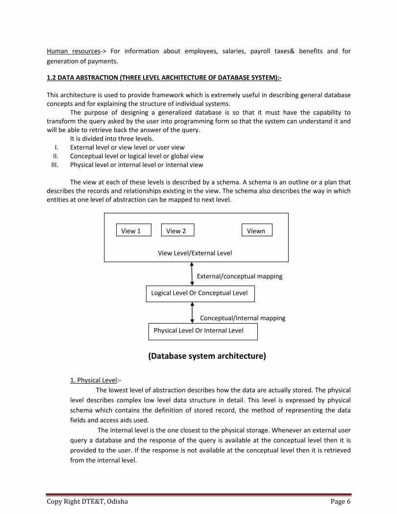
1.2 DATA ABSTRACTION (THREE LEVEL ARCHITECTURE OF DATABASE SYSTEM):- This architecture is used to provide framework which is extremely useful in describing general database concepts and for explaining the structure of individual systems. The purpose of designing a generalized database is so that it must have the capability to transform the query asked by the user into programming form so that the system can understand it and will be able to retrieve back the answer of the query. It is divided into three levels.
I. External level or view level or user view II. Conceptual level or logical level or global view
III. Physical level or internal level or internal view
The view at each of these levels is described by a schema. A schema is an outline or a plan that describes the records and relationships existing in the view. The schema also describes the way in which entities at one level of abstraction can be mapped to next level.
External/conceptual mapping
Conceptual/Internal mapping
(Database system architecture) 1. Physical Level:- The lowest level of abstraction describes how the data are actually stored. The physical level describes complex low level data structure in detail. This level is expressed by physical schema which contains the definition of stored record, the method of representing the data fields and access aids used. The internal level is the one closest to the physical storage. Whenever an external user query a database and the response of the query is available at the conceptual level then it is provided to the user. If the response is not available at the conceptual level then it is retrieved from the internal level.
View Level/External Level
View 1 View 2 Viewn
Logical Level Or Conceptual Level
Physical Level Or Internal Level

Copy Right DTE&T, Odisha Page 7
2. Logical Level:- i) The next higher level of abstraction describes what data are stored in the database and what relationship exists among those data. The logical level thus describes the entire database in terms of a small number of relatively simple structures. ii) It is defined by the logical schema. It describes all the records and relationships. There is one logical schema per database. iii) It also includes features that specify the checks to retain data consistency and integrity. iv) The conceptual schema is basically derived from the internal schema and it can be updated as per the demand of the users. 3. View Level:- i) The highest level of data abstraction describes only part of the entire database. The system may provide many views for the same database. ii) Each view is described by a schema called external schema. The external schema consists of the definition of logical records and relationships in the view level. iii) The external schema also contains the method of deriving the objects in the external view from the objects in the conceptual view. iv) It is the level closest to the users i.e. it deals with the way in which data is viewed by the users. v) All the types of database users use a particular language to query the database. The three level architecture is designed in such a way that each and every level maintains their abstraction by their own. The DBMS controls all the levels and the DBMS is basically controlled by the DBA.
1.3 DATABASE USERS:- There are five different types of database system users differentiated by the way they expect to interact with the system. Naive Users:-
They are unsophisticated users who interact with the system by invoking one of the application programs that have been written previously. Example:- ATM user
The typical user interface for a naive user is a forms interface where the user can fill in appropriate fields of the form. Naive users may also simply read reports generated from the database.
Application Programmers:- Application programmers are computer professionals who write application programs. Application programmers can choose from many tools like RAD tools, programming
languages, fourth generation languages etc. to develop user interfaces. Sophisticated Users:-
Sophisticated users interact with the system without writing programs. Instead they form their requests in database query language. They submit each such query to query processor whose function is to break down DML statements into instructions that the storage manager understands.
Analysts who submit queries to explore data in the database fall in this category.

Copy Right DTE&T, Odisha Page 8
Specialized Users:- Specialized users are sophisticated users who write specialized database applications
that do not fit into the traditional data processing framework. Among these applications are computer aided design systems, knowledge base& expert
systems that store data with complex structure(Example:- Graphics and audio data) and environment modeling systems
Database Administrators(DBA):- A person who has central control over the entire database system is called database administrator (DBA). The functions of DBA include
i. Schema definition ii. Storage structure and access method definition
iii. Schema and physical organization modification iv. Granting of authorization for data access v. Routine maintenance
1.4 DATA DEFINITION LANGUAGE (DDL):-
A database system provides a data definition language to specify the database schemas. For example the following SQL statement defines the account table.
Sql> create table account (accountno varchar2 (10), balance number); Execution of the above DDL statement creates the account table. In addition it updates a special set of tables called data dictionary.
DDL is used to define the database. This definition includes all the entity sets and their associated attributes as well as the relationship among the entity sets. It also includes any constraints that have to be maintained.
The DDL used at the external schema is called the view definition language (VDL) from where the defining process starts.
A data dictionary contains metadata. A database system consults data dictionary before reading or modifying actual data. The schema of a table is an example of a metadata i.e. data about data.
We specify the storage structure and access methods used by the database system by a set of statements in a special type of DDL called data storage and definition language (DSDL). These statements define the implementation details of the database schemas which are usually hidden from the users.
The DDL provides facilities to specify such consistency constraints. The database system checks these constraints every time the database is updated.

Copy Right DTE&T, Odisha Page 9
1.5 DATA DICTIONARY:- Information regarding the structure and usage of data contained in the database, the metadata
maintained in a data dictionary. The term system catalog also describes this metadata. The data dictionary which is a database itself documents the data.
Each database users can consult the data dictionary to learn what each piece of data and various synonyms of data fields mean.
In an integrated system (i.e. in system where the data dictionary is a part of the DBMS) the data dictionary stores information concerning the external, conceptual and internal levels of the database. It contains the source of each data field value, the frequency of its use and an audit trail concerning updates, including the who and when of each update.

Copy Right DTE&T, Odisha Page 10
CHAPTER-2
DATA MODELS 2.1 Data Independence:- Three levels of abstraction along with the mappings from internal to conceptual and from
conceptual to external level provide two distinct levels of data independence: logical data independence and physical data independence.
Logical data independence indicates that the conceptual schema can be changed without affecting the existing external schemas. The change would be absorbed by the mapping between the external and conceptual level.
Logical data independence also insulates application programs from operations such as combining two records into one or splitting an existing record into two or more records.
Logical data independence is achieved by providing the external level or user view of the database. The application programs or users see the database as described by their respective external views.
Physical data independence is achieved by the presence of the internal level of the database and the mapping or transformation from conceptual level of database to internal level.
The physical data independence criterion requires that the conceptual level does not specify storage structures or the access methods (indexing, hashing etc) used to retrieve the data from the physical storage medium.
Another aspect of data independence allows different interpretation of the same data. The storage of data is in bits and may change from EBCDIC to ASCII coding.
2.2 E-R DATA MODEL:- The E-R data model is based on a perception of a real world that consists of a collection of basic
objects called entities and of relationships among these objects. An entity is a ‘thing’ or ‘object’ in the real world that is distinguishable from other objects.
Example: - person, bank account etc. Entities are described in a database by a set of attributes. For example attributes like account
number and balance describe the entity bank account. In some cases an extra attribute is used to define uniquely an entity set.
A relationship is an association among several entities. For example a depositor relationship associates a customer with each account he has.
The set of all entities of same type and the set of all relationships of the same type are termed as entity set and relationship set respectively.
The overall logical structure (schema) of a database can be expressed graphically by an E-R diagram which is built up from the following components. Rectangles Entity Sets Ellipses Attributes Diamonds Relationships among entity sets

Copy Right DTE&T, Odisha Page 11
Lines Link attributes to entity sets and entity sets to relationships. Each component is labeled with the entity or relationship that it represents.
(E-R Diagram) In addition to entities and relationships, the E-R model represents certain constraints to which
the contents of a database must conform. One important constraint is mapping cardinalities, which express the number of entities to which another entity can be associated via a relationship set. For example, if each account must belong to only one customer the E-R model can express that constraint.
The E-R model is widely used in database design. 2.3 ENTITY SETS:- An entity is a thing or object in the real world that is distinguishable from all other objects.
Example:- Each person of an enterprise. An entity has a set of properties and values. For some set of properties may uniquely identify an
entity. Example:- Aadhar number An entity may be concrete such as a person or book or it may be abstract like a holiday or a
concept. An entity set is a set of entities of same type that share the same properties or attributes. For
example the set of all persons who are customers at a given bank can be defined as an entity set customer. The individual entities that constitute a set are said to be the extension of the entity set. For example the individual customers that constitute a set are the extension of the entity set customer.
Entity sets do not need to be disjoint. For example it is possible to define the entity set of all employees of a bank (employees) and the entity set of all customers of the bank.
2.4 ATTRIBUTES:- An entity is represented by a set of attributes. Attributes are descriptive properties possessed by
each member of an entity set. Each entity has a value for each of its attributes. For example a particular customer entity may
have the value 321-12 for customer id, value Anil for customer name etc. For each attribute there is a set of permitted values called domain or value set for that attribute.
Customer_id
Customer_name
Customer_street
Customer_city
Customer
Depositor
Accountno Balance
Account

Copy Right DTE&T, Odisha Page 12
Formally an attribute of an entity set is a function that maps from entity set into a domain. Since an entity set may have several attributes each entity can be described by a set of (attribute, data value) pairs, one pair for each attribute of the entity set.
An attribute is as used in the E-R model can be characterized by the following attribute types. Simple and Composite Attributes:- Attributes are said to be simple if they are not divided into subparts. For example customer id.
On the other hand composite attributes are divided into subparts. For example customer name, address.
Composite attributes help us to group together related attributes making the modeling cleaner. A composite attribute may appear as a hierarchy. For example address.
Single valued and multi valued attributes:- The attributes which have a single value for a particular entity is called a single valued attribute.
There may be instances where an attribute has a set of values for a specific entity. These are called multi valued entities. For example phone number.
Appropriate upper and lower bounds may be placed on the number of values in a multi valued attribute. For example a bank may limit the number of phone numbers recorded for a single customer to two.
Derived attribute:- The value for this type of attribute can be derived from the values of other related attributes or
entities. For example loan held. An attribute takes a null value when an entity does not have a value for it. The null value may
indicate not applicable i.e. the value does not exist for that entity. For example one may have no middle name.
2.3 RELATIONSHIP SETS:- A relationship is an association among several entities. A relationship set is a set of relationships of the same type. The association between entity sets is referred to as participation that is the entity sets E1, E2,
…………., En participate in a relationship set R. A relationship instance in an E-R schema represents an association between the named entities
of the real world enterprise that is being modeled. A relationship may also have attributes called descriptive attributes. Consider a relationship set
depositor with entity sets customer and account. We could associate the attribute access date to that relationship to specify the most recent date on which the customer accessed an account.
A relationship instance in a given relationship set must be uniquely identifiable from its participating entities, without using descriptive attributes. For example instead of using a single access date we use access dates.
However there can be more than one relationship set involving the same entity set. For example guarantor in customer –loan relationship.
One that involves two entity sets is called binary relationship. Most of the relationship sets in a database system are binary.
The relationship set works on among employees, branch and job is an example of ternary relationship.
The number of entity sets that participate in a relationship set is also called the degree of relationship set. A binary relationship set is of degree two and a ternary relationship set is of degree three.
Copy Right DTE&T, Odisha Page 13
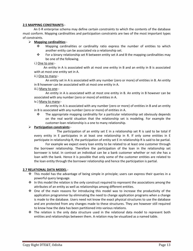
2.5 MAPPING CONSTRAINTS:- An E-R enterprise schema may define certain constraints to which the contents of the database must conform. Mapping cardinalities and participation constraints are two of the most important types of constraints. Mapping cardinalities:-
Mapping cardinalities or cardinality ratio express the number of entities to which another entity can be associated via a relationship set.
For a binary relationship set R between entity set A and B the mapping cardinalities may be one of the following.
i.) One to one:- An entity in A is associated with at most one entity in B and an entity in B is associated with at most one entity set in A. ii.) One to many:- An entity set in A is associated with any number (zero or more) of entities in B. An entity in B however can be associated with at most one entity in A. iii.) Many to one:- An entity in A is associated with at most one entity in B. An entity in B however can be associated with any number (zero or more) of entities in A. iv.) Many to many:- An entity in A is associated with any number (zero or more) of entities in B and an entity in B is associated with any number (zero or more) of entities in A. The appropriate mapping cardinality for a particular relationship set obviously depends
on the real world situation that the relationship set is modeling. For example the customer-loan relationship is a one to many relationship.
Participation constraints:- The participation of an entity set E in a relationship set R is said to be total if every entity in E participates in at least one relationship in R. If only some entities in E participate in relationship R, the participation of entity set E in relationship R is said to be partial. For example we expect every loan entity to be related to at least one customer through the borrower relationship. Therefore the participation of the loan in the relationship set borrower is total. In contrast an individual can be a bank customer whether or not she has a loan with the bank. Hence it is possible that only some of the customer entities are related to the loan entity through the borrower relationship and hence the participation is partial. 2.7 RELATIONAL DATA MODEL:- This model has the advantage of being simple in principle; users can express their queries in a
powerful query language. In this model the relation is the only construct required to represent the associations among the
attributes of an entity as well as relationships among different entities. One of the main reasons for introducing this model was to increase the productivity of the
application programmer by eliminating the need to change application programs when a change is made to the database. Users need not know the exact physical structures to use the database and are protected from any changes made to these structures. They are however still required to know how the data has been partitioned into various relations.
The relation is the only data structure used in the relational data model to represent both entities and relationships between them. A relation may be visualized as a named table.
Copy Right DTE&T, Odisha Page 14
Rows of the relation are referred to as tuples of the relation and the columns are its attributes. Each attribute of a relation has a distinct name. The values for an attribute or a column are drawn from a set of values known as domain.
2.8 NETWORK DATA MODEL:- The network data model was formalized in the late 1960’s by the Database Task Group of
Conference on data system languages (DBTG/CODASYL). Hence it is also known as DBTG model. The network model uses two different data structures to represent the database entities and
relationship between the entities named record type and set type. A record type is used to represent an entity type. It is made up of a number of data items that represents the attributes of an entity.
A set type is used to represent a directed relationship between two record types, the so called owner record type and the member record type. The set type like the record type is named and specifies that there is a one to many relationship
(1:M) between the owner and member record types. The set type can have more than one record type as its member, but only one record type is allowed to be the owner in a given set type.
A database could have one or more occurrences of each of its record types and set types. An occurrence of a set type consists of an occurrence of the owner record type and any number of occurrences of each of its member record type. A record type can’t be a member of two distinct occurrences of the same type.
To avoid the confusion inherent in the use of the word ‘set’ to describe the mechanism for showing relationship in the network model, the other terms suggested are co set, fan set, owner coupled set, CODASYL set, DBTG set etc.
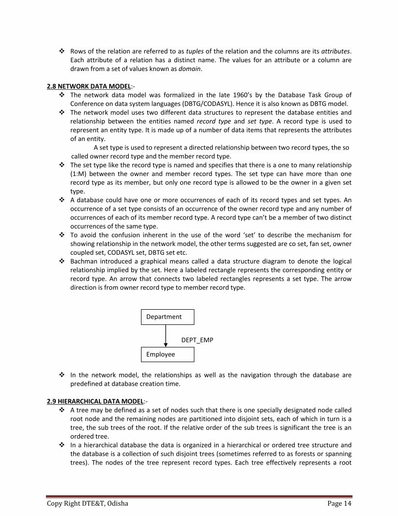
Bachman introduced a graphical means called a data structure diagram to denote the logical relationship implied by the set. Here a labeled rectangle represents the corresponding entity or record type. An arrow that connects two labeled rectangles represents a set type. The arrow direction is from owner record type to member record type.
DEPT_EMP In the network model, the relationships as well as the navigation through the database are
predefined at database creation time. 2.9 HIERARCHICAL DATA MODEL:- A tree may be defined as a set of nodes such that there is one specially designated node called
root node and the remaining nodes are partitioned into disjoint sets, each of which in turn is a tree, the sub trees of the root. If the relative order of the sub trees is significant the tree is an ordered tree.
In a hierarchical database the data is organized in a hierarchical or ordered tree structure and the database is a collection of such disjoint trees (sometimes referred to as forests or spanning trees). The nodes of the tree represent record types. Each tree effectively represents a root
Department
Employee

Copy Right DTE&T, Odisha Page 15
record type and all its dependent record types. If we define the root record type at level 0, then the level of its dependent record types can be defined at level 1. The dependents of the record types at level 1 are said to be at level 2 and so on.
An occurrence of a hierarchical tree type consists of one occurrence of the root record type along with zero or more occurrences of its dependent sub tree types. Each dependent sub tree is in turn, hierarchical and consists of a record type as its root node.
In a hierarchical model no dependent record can occur without its parent record occurrence. Furthermore no dependent record occurrence may be connected to more than one parent record occurrence.
A hierarchical model can represent a one to many relationships between two entities where the two are respectively parent and child. However to represent many to many relationship requires duplication of one of the record types corresponding to one of the entities involved in this relationship. Note that such duplications lead to inconsistencies when only one copy of a duplicate record is updated.
Copy Right DTE&T, Odisha Page 16
CHAPTER-3
RELATIONAL DATABASE
QUERY LANGUAGE:- A query language is a language in which a user requests information from the database. These
languages are usually on a level higher than that of a standard programming language. Query languages can be categorized as either procedural or non-procedural. In a procedural
language the user instructs the system to perform a sequence of operations on the database to compute the desired result. In a non-procedural language the user describes the desired information without giving a specific procedure for obtaining that information.
3.1 RELATIONAL ALGEBRA:- The relational algebra is a procedural query language. It consists of a set of operations that take
one or two relations as its operands and produces a new relation as its result. The fundamental operations in the relational algebra are select, project, union, set difference,
rename and Cartesian product. In addition to the fundamental operations there are several other operations namely set
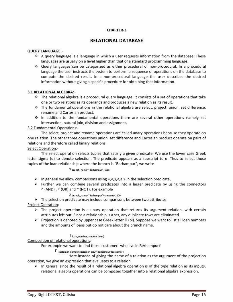
intersection, natural join, division and assignment. 3.2 Fundamental Operations:- The select, project and rename operations are called unary operations because they operate on one relation. The other three operations union, set difference and Cartesian product operate on pairs of relations and therefore called binary relations. Select Operation:- The select operation selects tuples that satisfy a given predicate. We use the lower case Greek letter sigma (σ) to denote selection. The predicate appears as a subscript to σ. Thus to select those tuples of the loan relationship where the branch is “Berhampur”, we write σ branch_name=”Berhampur” (loan)
In general we allow comparisons using =,≠,≤,<,≥,> in the selection predicate, Further we can combine several predicates into a larger predicate by using the connectors
˄ (AND) , ˅ (OR) and ~ (NOT). For example σ branch_name=”Berhampur”^ amount>1200
The selection predicate may include comparisons between two attributes. Project Operation:- The project operation is a unary operation that returns its argument relation, with certain
attributes left out. Since a relationship is a set, any duplicate rows are eliminated. Projection is denoted by upper case Greek letter Π (pi). Suppose we want to list all loan numbers
and the amounts of loans but do not care about the branch name. Π loan_number, amount (loan)
Composition of relational operations:- For example we want to find those customers who live in Berhampur? Π customer_name(σ customer_city=”Berhampur”(customer))
Here instead of giving the name of a relation as the argument of the projection operation, we give an expression that evaluates to a relation. In general since the result of a relational algebra operation is of the type relation as its inputs,
relational algebra operations can be composed together into a relational algebra expression.

Copy Right DTE&T, Odisha Page 17
Composing relational algebra operations into relational algebra expressions is just like composing arithmetic operations i.e. Inner parentheses will be evaluated first and then the outer parentheses and so on.
Union operation:- Consider a query to find the names of all bank customers who have either an account or a loan
account or both. The customer relation does not contain information about loan and the loan relation does not contain information about customer. So to find all the customer of a particular bank we have to join both relations by the following projection operation. Π customer_name(depositor) U Π borrower_name(loan)
To have union operation we require two conditions. 1. The relations R and S must be of same arity i.e. they must have same number of
attributes. 2. The domains of the ith attribute of R and the ith attribute of S must be same for all i.
Set Difference operation:- The set difference operation is denoted by “–“allows us to find tuples that are in one relation
but not are in the other one. The expression R-S produces a relation containing those tuples that are in R but not in S
We can find all customers of the bank who have an account but not a loan. Π customer_name(deositor)-Π customer_name(borrower)
We must ensure that set difference are taken between compatible relations. Therefore a set difference operation R-S to be valid we require that the relations R and S be of same arity and the domains of ith attribute of R and the ith attribute of S be same for all i.
Cartesian product operation:- The Cartesian product operation denoted by “X” allows us to combine information from any two
relations. We write the Cartesian product of relations R1 and R2 as R1 X R2 A relation is by definition a subset of a Cartesian product of a set of domains. However since the same attribute name may appear in both R1 and R2 we need to devise a
naming schema to distinguish between these attributes. We do it by attaching to an attribute the name of the relation from which the attribute originally
came. For example the relational schema R= borrower X depositor is (depositor.name, depositor.accno, borrower.name, borrower.loan no, borrower.accno)
Set intersection operation:- We want to find out the customers who have both a loan and an account. Using set intersection
operation we write Π depositor_name(depositor)∩ Π borrower_name(borrower)
We can rewrite any relational algebra expression that uses set intersection operation with a pair of set difference operation. R∩S=R-(R-S)
Natural Join operation:- The natural join is a simple operation that allows us to combine certain selections and a
Cartesian product into one operation. It is denoted by the join symbol .The natural join operation forms a Cartesian product of its two arguments, performs a selection forcing equality on those attributes that appear in both relation schemas and finally removes duplicate attributes.

Copy Right DTE&T, Odisha Page 18
Although the definition of natural join is complicated the operation is easy to apply. For example find the names of all customers who have a loan in the bank and find the amount of loan. Π customer_name, amount (depositor borrower) Definition of natural join:- Consider two relations r(R) and s(S). The natural join of r and s, denoted by r s formally defined as follows. r s= Π RUS(σ r.A1=s.A1˄r.A2=S.A2˄…………………˄r.An=s.An)
Where R∩S= {A1, A2, A3,…………………., An} The natural join is associative i.e. if there are three relations P, Q and R, then associativity shows
that ( P Q) R = P (Q R)

Copy Right DTE&T, Odisha Page 19
CHAPTER-4
NORMALIZATION IN RELATIONAL SYSTEM
Keys:- A key allows us to identify a set of attributes that suffice to distinguish entities from each other.
Keys also help to uniquely identify relationships and thus to distinguish relationships from each other.
A super key is a set of one or more attributes that taken collectively allow us to identify uniquely an entity in the entity set. For example the customer _id attribute of the entity set customer and customer_ name & customer_ id attributes of the entity set customer.
The concept of a super key is not sufficient for our purpose, since we can see that a super key may contain extra attributes. So we are interested in super keys for which no proper subset is a super key. Such minimal super keys are called candidate keys. It is possible that several distinct sets of attributes could serve as a candidate key. For example customer_ name, customer_ street
We use the term primary key to denote a candidate key that is choosen by the database engineer as the principal means of identifying entities within an entity set.
4.1 FUNCTIONAL DEPENDENCIES:- Functional dependencies play a key role in differentiating good database design from bad
database design. Functional dependencies are constraints on the set of legal relations. They allow us to express
facts about the enterprise that we are modeling with our database. The notion of functional dependency generalizes the notion of super key. Consider a relation
schema R and let αϹ R and βϹ R. The functional dependency α β holds on schema R, if any legal relation r(R), for all pairs of tuples t1 and t2 in r such that t1 [α] = t2 [α], it is also the case that t1 [β] = t2 [β]
Using functional dependency notation, we say that k is a super key of R if k → R that is k is a super key if whenever t1 [k] = t2 [k], it is also the case that t1 [R] = t2 [R] (that is t1 = t2)
Functional dependencies allow us to express constraints that we cannot express through super keys. Consider the schema Loan_ info_ schema = (loan_ number, branch_ name, customer_ name, amount) The set of functional dependency loan_ number → amount loan_ number → branch_ name However we could not expect the functional dependency loan_ number → customer_ name to hold, since in general a given loan can be made to more than one customer.
We shall use functional dependencies in two ways. 1. To test relations to see whether they are legal under a given set of functional
dependencies. If a relation R is legal under a set F of functional dependencies we say that R satisfies F.
2. To specify constraints on the set of legal relations. We shall thus concern ourselves with only those relations that satisfy a given set of functional dependencies. If we wish to constraint ourselves to relations on schema R that satisfy a set F of functional dependencies, we say that F holds on R.

Copy Right DTE&T, Odisha Page 20
4.2 LOSS LESS DECOMPOSITION:- When we decompose a relation into a number of smaller relations, it is crucial that the
decomposition be lossless. We must first present criteria for determining whether a composition is lossy.
Let R be relation schema and F be a set of functional dependencies on R. Let R1 and R2 form a decomposition of R. This composition is a loss less join decomposition of R if at least one of the following functional dependencies is in F+ :
(i) R1 ∩R2 → R1 (ii) R1 ∩R2 → R2
In other words if R1 ∩ R2 forms a super key of either R1 or R2 the decomposition of R is a loss less decomposition.
For the general case of decomposition of a relation into multiple parts at once the test for lossless join decomposition is more complicated.
While the test for binary decomposition is clearly a sufficient condition for loss less join, it is a necessary condition only if all constraints are functional dependencies.
NORMALIZATION
If a database design is not perfect it may contain anomalies, which are like a bad dream for database itself. Managing a database with anomalies is next to impossible.
Update anomalies: if data items are scattered and are not linked to each other properly, then there may be instances when we try to update one data item that has copies of it scattered at several places, few instances of it get updated properly while few are left with there old values. This leaves database in an inconsistent state.
Deletion anomalies: we tried to delete a record, but parts of it left undeleted because of unawareness, the data is also saved somewhere else.
Insert anomalies: we tried to insert data in a record that does not exist at all. Normalization is a method to remove all these anomalies and bring database to consistent state and free from any kinds of anomalies.
4.3 IMPORTANCE OF NORMALIZATION:- Searching, sorting, and creating indexes is faster, since tables are narrower, and more rows fit
on a data page. You usually have more tables. You can have more clustered indexes (one per table), so you get more flexibility in tuning
queries. Index searching is often faster, since indexes tend to be narrower and shorter. More tables allow better use of segments to control physical placement of data. You usually have fewer indexes per table, so data modification commands are faster. Fewer null values and less redundant data, making your database more compact. Triggers execute more quickly if you are not maintaining redundant data. Data modification anomalies are reduced. Normalization is conceptually cleaner and easier to maintain and change as your needs change. The cost of finding rows already in the data cache is extremely low. Avoids data modification (INSERT/DELETE/UPDATE) anomalies as each data item lives in one
place. Fewer null values and less opportunity for inconsistency.
Copy Right DTE&T, Odisha Page 21
A better handle on database security. Increased storage efficiency. The normalization process helps maximize the use of clustered indexes, which is the most
powerful and useful type of index available. As more data is separated into multiple tables because of normalization, the more clustered indexes become available to help speed up data access.
Disadvantages of normalization:- Requires much more CPU, memory, and I/O to process thus normalized data gives reduced
database performance. Requires more joins to get the desired result. A poorly-written query can bring the database
down. Maintenance overhead i.e. the higher the level of normalization, the greater the number of
tables in the database.
4.4 FIRST NORMAL FORM(1NF):- The first of the normal forms that we study, first normal form imposes a very basic requirement
on relations; unlike the other normal forms, it does not require additional information such as functional dependency.
A domain is atomic if elements of the domain are considered to be individual units. We say that a relation schema R is in first normal form (1NF) if the domains of all the attributes of R are atomic.
In other words only one value is associated with each attribute and the value is not set of values or list of values.
A database schema is in first normal form if every relation schema included in the database schema is in 1NF.
The first normal form pertains to the tabular format of the relation. Sometimes non atomic values can be useful. For example composite valued attributes and set
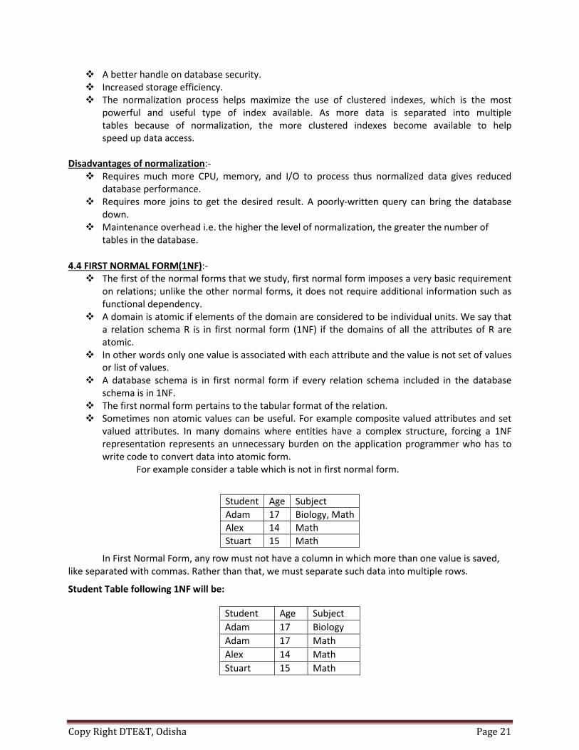
valued attributes. In many domains where entities have a complex structure, forcing a 1NF representation represents an unnecessary burden on the application programmer who has to write code to convert data into atomic form. For example consider a table which is not in first normal form.
In First Normal Form, any row must not have a column in which more than one value is saved, like separated with commas. Rather than that, we must separate such data into multiple rows.
Student Table following 1NF will be:
Student Age Subject Adam 17 Biology, Math Alex 14 Math Stuart 15 Math
Student Age Subject Adam 17 Biology Adam 17 Math Alex 14 Math Stuart 15 Math

Copy Right DTE&T, Odisha Page 22
Using the First Normal Form, data redundancy increases, as there will be many columns with same data in multiple rows but each row as a whole will be unique.
SECOND NORMAL FORM (2NF):- A relation scheme R<S, F> is in 2NF if it is in 1NF and if all non prime attributes are fully
functional dependent on the relation keys. A database schema is in 2NF if every relation schema included in the database schema is in 2NF A 2NF does not permit partial dependency between a non prime attribute and the relation keys. Even though 2NF does not permit partial dependency between a non prime attribute and the
relation keys it does not rule out the possibility that a non prime attribute may also be functionally dependent on another non prime attribute. This type of dependency between non prime attributes also causes anomalies.
In example of First Normal Form there are two rows for Adam, to include multiple subjects that he has opted for. While this is searchable, and follows First normal form, it is an inefficient use of space. Also in the above Table in First Normal Form, while the candidate key is {Student, Subject}, Age of Student only depends on Student column, which is incorrect as per Second Normal Form. To achieve second normal form, it would be helpful to split out the subjects into an independent table, and match them up using the student names as foreign keys. New Student Table following 2NF will be :
In Student Table the candidate key will be Student column, because all other column i.e Age is dependent on it.
New Subject Table introduced for 2NF will be:
In Subject Table the candidate key will be {Student, Subject} column. Now, both the above tables qualify for Second Normal Form and will never suffer from Update Anomalies. Although there are a few complex cases in which table in Second Normal Form suffers Update Anomalies, and to handle those scenarios Third Normal Form is there THIRD NORMAL FORM (3NF):- BCNF requires that all non trivial dependencies of the form α → β, where α is a super key. Third
normal form (3NF) relaxes this constraint slightly by allowing certain non trivial functional dependencies whose left side is not a super key.
Student Age Adam 17 Alex 14 Stuart 15
Student Subject Adam Biology Adam Math Alex Math Stuart Math

Copy Right DTE&T, Odisha Page 23
A relation schema R is in third normal form with respect to a set F of functional dependencies if, for all functional dependencies in F+ of the form α → β, where α Ϲ R and β Ϲ R, at least one of the following holds:
1. α →β is a trivial functional dependency 2. α is a super key for R 3. Each attribute A in β – α is contained in a candidate key for R
Note that the third condition above does not say that a single candidate key must contain all the attributes in β – α; each attribute A in β – α may be contained in a different candidate key.
Third Normal form applies that every non-prime attribute of table must be dependent on primary key. The transitive functional dependency should be removed from the table. The table must be in Second Normal form. For example, consider a table with following fields.
Student_Detail Table :
Student_id Student_name DOB Street City State PIN
In this table Student_id is Primary key, but street, city and state depends upon PIN. The dependency between PIN and other fields is called transitive dependency. Hence to apply 3NF, we need to move the street, city and state to new table, with PIN as primary key.
New Student_Detail Table :
Student_id Student_name DOB PIN
Address Table:
PIN Street City State
The advantage of removing transitive dependency is:-
Amount of data duplication is reduced. Data integrity achieved.
BOYCE- CODD NORMAL FORM (BCNF):- Boyce- Codd normal form eliminates all redundancy that can be discovered based on functional
dependencies. A relational schema R is in BCNF with respect to a set F of functional dependencies in F+ of the
form α → β, where αϹ R and β Ϲ R, at least one of the following holds: 1. α →β is a trivial functional dependency (that is β Ϲ α) 2. α is a super key for schema R
A database design is in BCNF if each member of the set of relation schemas that constitute the design is in BCNF.
When we decompose a schema that is not in BCNF, it may be that one or more of the resulting schemas are not in BCNF. In such cases further decomposition is required, the eventful result of which is a set of BCNF schemas.

Copy Right DTE&T, Odisha Page 24
The BCNF imposes a stronger constraint on the types of functional dependencies allowed in a relation. The only non trivial functional dependencies allowed in a relation. The only non trivial functional dependencies allowed in the BCNF are those functional dependencies whose determinants are candidate super keys of the relation.
Any schema that satisfies BCNF also satisfies 3NF, since each of its functional dependencies would satisfy one of the first two alternatives. BCNF is therefore a more restrictive normal form than is 3NF.
A 3NF table which does not have multiple overlapping candidate keys is said to be in BCNF.
In the above normalized tables in 3NF, Student_id is super-key in Student_Detail relation and PIN is super-key in Address relation. So,
Student_id → Student_name, DOB, PIN And PIN → Street, City, State
confirms, that both relations are in BCNF.
Copy Right DTE&T, Odisha Page 25
CHAPTER-5
STRUCTURED QUERY LANGUAGE
5.1 QUERY LANGUAGE:- A query language is a language in which a user requests information from the database. These
languages are usually on a level higher than that of a standard programming language. Query languages can be categorized as either procedural or non-procedural. In a procedural
language the user instructs the system to perform a sequence of operations on the database to compute the desired result. In a non-procedural language the user describes the desired information without giving a specific procedure for obtaining that information.
5.2 QUERIES IN SQL:- Table:- A table is a database object that holds user data. The simplest analogy is to think of a table as a
spread sheet The columns of a table are associated with a specific data type. Oracle ensures that only data which is identical to the data type of the column will be stored
within the column. Data type:-
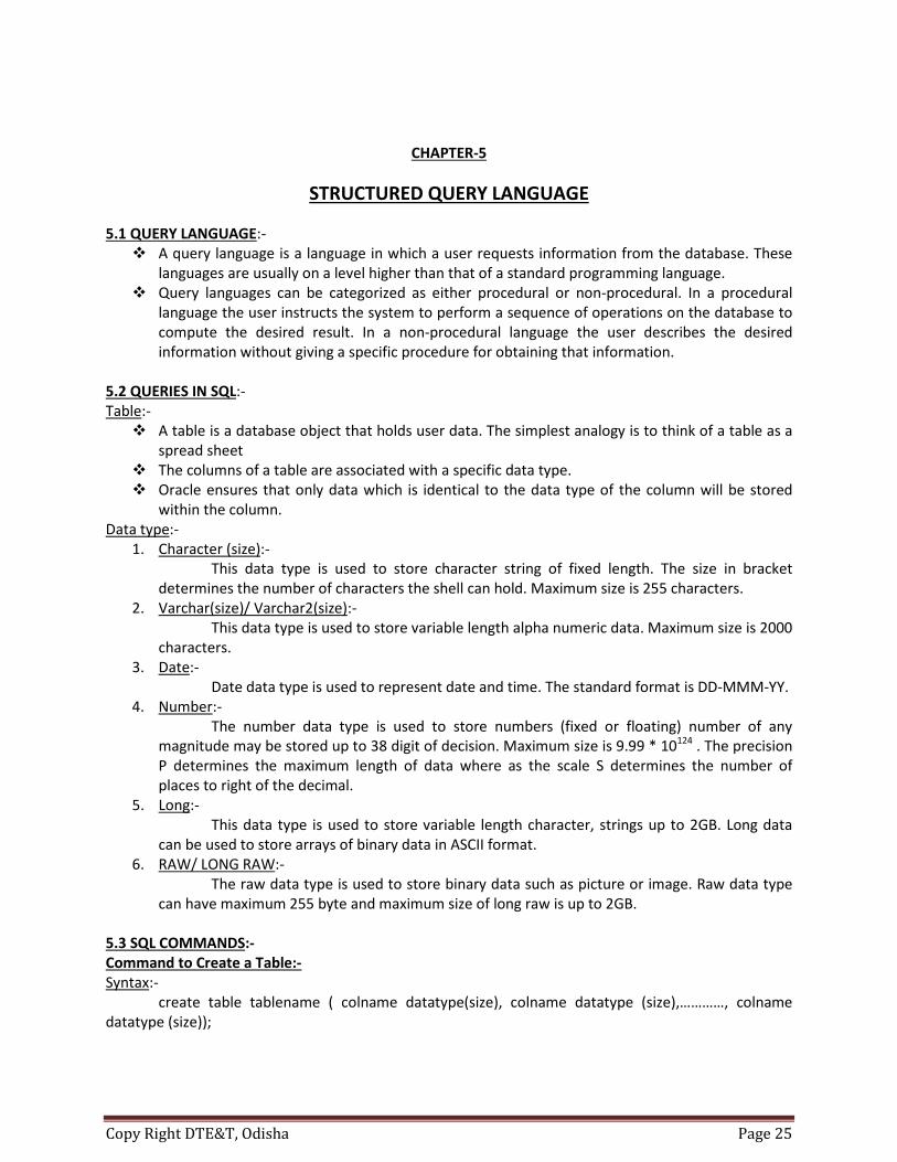
1. Character (size):- This data type is used to store character string of fixed length. The size in bracket determines the number of characters the shell can hold. Maximum size is 255 characters.
2. Varchar(size)/ Varchar2(size):- This data type is used to store variable length alpha numeric data. Maximum size is 2000 characters.
3. Date:- Date data type is used to represent date and time. The standard format is DD-MMM-YY.
4. Number:- The number data type is used to store numbers (fixed or floating) number of any magnitude may be stored up to 38 digit of decision. Maximum size is 9.99 * 10124 . The precision P determines the maximum length of data where as the scale S determines the number of places to right of the decimal.
5. Long:- This data type is used to store variable length character, strings up to 2GB. Long data can be used to store arrays of binary data in ASCII format.
6. RAW/ LONG RAW:- The raw data type is used to store binary data such as picture or image. Raw data type can have maximum 255 byte and maximum size of long raw is up to 2GB.
5.3 SQL COMMANDS:- Command to Create a Table:- Syntax:- create table tablename ( colname datatype(size), colname datatype (size),…………, colname datatype (size));

Copy Right DTE&T, Odisha Page 26
Example:- Create table student(rollno varchar2(20), name varchar2(30), address varchar2(50),semester varchar2(10)); To view the structure of a table:- Syntax:- Sql> desc table name; Example:- Desc student;
Column name Data type size Rollno varchar2 20 Name varchar2 30 Address varchar2 50 Semester varchar2 10
Command to insert data into a table:- While inserting a single row of data into a table, the insert operation first creates a new row (empty in the database table) and then loads the value passed into the column specified. Syntax:- Insert into table name (col1, col2, col3,………., coln) values (expr1, expr2, expr3,…….., exprn); Example: Insert into student (‘f1201207005’,’radhika’,’bbsr’,’3rd cse’); Insert into student (‘f1201207002’,’rupak’,’ctc’,’5th cse’); Insert into student (‘f1201207003’,’jyoti’,’rkl’,’5th it’); Insert into student (‘f1201207008’,’ajay’,’bam’,’3rd it’); Insert into student (‘f1201207001’,’manoj’,’khd’,’5th cse’); Viewing data of a table:- In order to view the total data of the table the syntax is as follows. Syntax:- Sql> Select * from table name; Example:- Select * from student;
rollno name address semester f1201207005 radhika bbsr 3rd cse f1201207002 rupak ctc 5th cse f1201207003 Jyoti rkl 5th it f1201207008 Ajay bam 3rd it f1201207001 manoj khd 5th cse
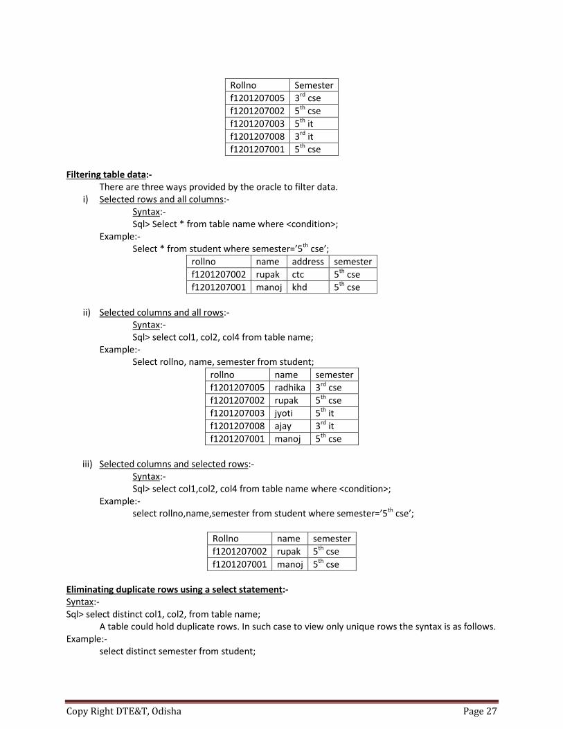
In order to view the partial column data we have the following syntax. Syntax:- Sql> Select col1, col2, col5 from table name; Example:- Select rollno, semester from student;
Copy Right DTE&T, Odisha Page 27
Rollno Semester f1201207005 3rd cse f1201207002 5th cse f1201207003 5th it f1201207008 3rd it f1201207001 5th cse
Filtering table data:- There are three ways provided by the oracle to filter data.
i) Selected rows and all columns:- Syntax:- Sql> Select * from table name where <condition>; Example:- Select * from student where semester=’5th cse’;
rollno name address semester f1201207002 rupak ctc 5th cse f1201207001 manoj khd 5th cse
ii) Selected columns and all rows:-
Syntax:- Sql> select col1, col2, col4 from table name;
Example:- Select rollno, name, semester from student;
rollno name semester f1201207005 radhika 3rd cse f1201207002 rupak 5th cse f1201207003 jyoti 5th it f1201207008 ajay 3rd it f1201207001 manoj 5th cse
iii) Selected columns and selected rows:- Syntax:- Sql> select col1,col2, col4 from table name where <condition>; Example:- select rollno,name,semester from student where semester=’5th cse’;
Rollno name semester f1201207002 rupak 5th cse f1201207001 manoj 5th cse
Eliminating duplicate rows using a select statement:- Syntax:- Sql> select distinct col1, col2, from table name; A table could hold duplicate rows. In such case to view only unique rows the syntax is as follows. Example:- select distinct semester from student;

Copy Right DTE&T, Odisha Page 28
semester 3rd cse 5th cse 5th it 3rd it
Syntax:- Sql> select distinct * from table name; Example:- select distinct * from student; rollno name address semester f1201207005 radhika bbsr 3rd cse f1201207002 rupak ctc 5th cse f1201207003 jyoti rkl 5th it f1201207008 ajay bam 3rd it f1201207001 manoj khd 5th cse f1201207003 jyoti rkl 5th it (Base Table) (Resulting Table) Sorting data in a table:- Oracle allows data from a table to the view in a sorted order. The rows retrieved from the table will be sorted in either ascending or descending order. In case
if there is no mention of the sorting order, the oracle engine sorts the data in ascending order by default.
Syntax:- Sql> select * from table name order by col1, col2 desc; Example:- Select * from student order by rollno desc;
rollno name address semester f1201207008 Ajay bam 3rd it f1201207005 radhika bbsr 3rd cse f1201207003 Jyoti rkl 5th it f1201207002 rupak ctc 5th cse f1201207001 manoj khd 5th cse
Creating a table from another table:- Syntax:- Sql> create table new table name (col1,col2,col3,col4) as select col1,col2, col3, col4 from old table name; Example:- Create table course (regdno, sname, address, sem) as select rollno, name, address, semester from student;
rollno name address semester f1201207005 radhika bbsr 3rd cse f1201207002 rupak ctc 5th cse f1201207003 jyoti rkl 5th it f1201207008 ajay bam 3rd it f1201207001 manoj khd 5th cse

Copy Right DTE&T, Odisha Page 29
regdno sname address sem f1201207008 ajay bam 3rd it f1201207005 radhika bbsr 3rd cse f1201207003 jyoti rkl 5th it f1201207002 rupak ctc 5th cse f1201207001 manoj khd 5th cse
Inserting data into a table created from another table:- Syntax:- Sql> insert into new table name select col1, col2, col3, col4 from old table name where<condition>; Example:- Insert into course select rollno, name, address, semester from student where name=’ajay’;
regdno sname address sem f1201207008 ajay bam 3rd it
Deleting data from a table:- To remove all the rows from a table the syntax is as follows
Syntax:- Sql> delete from table name; Example:- delete from student; To remove a set of rows from a table the syntax is as follows
Syntax:- Sql> delete from table name where <condition>; Example:- delete from student where name=’radhika’;
rollno name address semester f1201207008 Ajay bam 3rd it f1201207003 jyoti rkl 5th it f1201207002 rupak ctc 5th cse f1201207001 manoj khd 5th cse
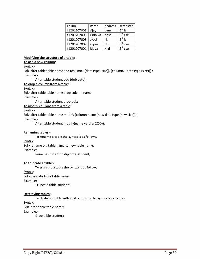
Updating the contents of a table:- The update command is used to change or modify data value of a table. Syntax:- Sql> update table name set col1=<expression>, col2=<expression>; Example:- Update student set address=’bam’; To update records conditionally we can use the following syntax. Syntax:- Sql> update table name set col. name=<expression> where <condition>; Example:- Update student set name=’bidya’ where rollno=’f1201207001’;
Copy Right DTE&T, Odisha Page 30
rollno name address semester f1201207008 Ajay bam 3rd it f1201207005 radhika bbsr 3rd cse f1201207003 Jyoti rkl 5th it f1201207002 rupak ctc 5th cse f1201207001 bidya khd 5th cse
Modifying the structure of a table:- To add a new column:- Syntax:- Sql> alter table table name add (column1 (data type (size)), (column2 (data type (size))) ; Example:- Alter table student add (dob date); To drop a column from a table:- Syntax:- Sql> alter table table name drop column name; Example:- Alter table student drop dob; To modify columns from a table:- Syntax:- Sql> alter table table name modify (column name (new data type (new size))); Example:- Alter table student modify(name varchar2(50)); Renaming tables:- To rename a table the syntax is as follows. Syntax:- Sql> rename old table name to new table name; Example:- Rename student to diploma_student; To truncate a table:- To truncate a table the syntax is as follows. Syntax:- Sql> truncate table table name; Example:- Truncate table student; Destroying tables:- To destroy a table with all its contents the syntax is as follows. Syntax:- Sql> drop table table name; Example:- Drop table student;

Copy Right DTE&T, Odisha Page 31
CHAPTER-6
TRANSACTION PROCESSING CONCEPTS 6.1 TRANSACTION PROCESSING:- A transaction is a program unit whose execution may change the contents of a database If the database was in a consistent state before a transaction, then on completion of the
transaction the database will be in a consistent state. This requires that the transaction be considered atomic, it is executed successfully or in case of
errors the user can view the transaction as not having been executed at all. 6.2 TRANSACTION CONCEPT:- States of transaction:- A transaction can be considered to be an atomic operation by the user but in reality it goes through a number of states during its life time.
Okay to Commit Database Modified
No errors
System detects Consistent error State
Error System Detected by Initiated Transactions Consistent State
Transaction Initiated Database Modified
A transaction can end in three possible ways. It can end after a commit operation (a successful termination). It can detect an error during its processing and decide to abort itself by performing a
Start
Commit
Commit
Modify
Abort
End of transaction
Error
Roll back

Copy Right DTE&T, Odisha Page 32
rollback operation (a suicidal termination). The DBMS or operating system can force it to be aborted for one reason or another (a murderous termination). We assume that the database is in a consistent state before a transaction starts. A transaction starts when the first statement of transaction is executed; it becomes active and we assume that it is in modify state when it modifies the database.
At the end of modify state there is a transition into one of the following states: start to commit, abort or error. If the transaction completes the modification state satisfactorily, it enters the start to commit state where it instructs the DBMS to reflect the changes made by it into a database. Once all the changes made by transaction are propagated to the database, the transaction is said to be in commit state and from there the transaction is terminated, the database is once again in a consistent state. In the interval between start to commit state and commit state some of the data changed by transaction in the buffer may or may not have been propagated to the database on the non volatile storage. There is a possibility that all modifications done by the transaction cannot propagated to the database due to conflicts or hardware failures. In this case the system forces the transaction to the abort state. The abort state could also be entered from the modify state if there are system errors for example division by zero. If the system aborts a transaction, it may have to initiate a rollback to undo partial changes made by the transaction. An aborted transaction that made no changes to the database is terminated without the need of the rollback. A transaction that on execution of its last statement enters the start to commit state to commit state and from there commit state is guaranteed and the modifications made are propagated to the database. The transaction outcome may either be successful (if the transaction goes through commit state), suicidal ( if the transaction goes through the rollback state ) and murderer (if the transaction goes through abort state). In the last two cases there is no trace of the transaction left in the database and only the log indicates that the transaction was ever run. Any message given to the user by the transaction must be delayed till the end of the transaction at which point the user can be notified as to success or failure and in the later case the reasons for failure.
6.3 Properties of transaction:- The database system must maintain the following properties of transactions to show all the characteristics. The properties referred to ACID (atomicity, consistency, isolation and durability) test represent the transaction paradigm.
Copy Right DTE&T, Odisha Page 33
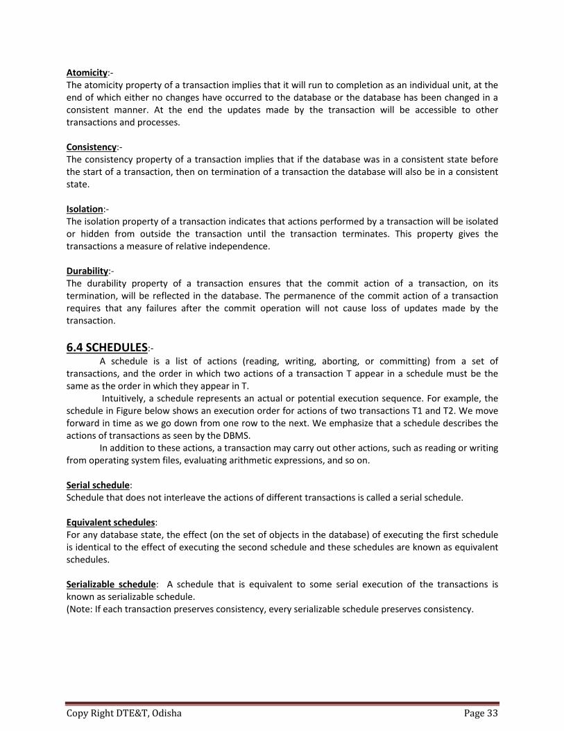
Atomicity:- The atomicity property of a transaction implies that it will run to completion as an individual unit, at the end of which either no changes have occurred to the database or the database has been changed in a consistent manner. At the end the updates made by the transaction will be accessible to other transactions and processes. Consistency:- The consistency property of a transaction implies that if the database was in a consistent state before the start of a transaction, then on termination of a transaction the database will also be in a consistent state. Isolation:- The isolation property of a transaction indicates that actions performed by a transaction will be isolated or hidden from outside the transaction until the transaction terminates. This property gives the transactions a measure of relative independence. Durability:- The durability property of a transaction ensures that the commit action of a transaction, on its termination, will be reflected in the database. The permanence of the commit action of a transaction requires that any failures after the commit operation will not cause loss of updates made by the transaction. 6.4 SCHEDULES:- A schedule is a list of actions (reading, writing, aborting, or committing) from a set of transactions, and the order in which two actions of a transaction T appear in a schedule must be the same as the order in which they appear in T. Intuitively, a schedule represents an actual or potential execution sequence. For example, the schedule in Figure below shows an execution order for actions of two transactions T1 and T2. We move forward in time as we go down from one row to the next. We emphasize that a schedule describes the actions of transactions as seen by the DBMS. In addition to these actions, a transaction may carry out other actions, such as reading or writing from operating system files, evaluating arithmetic expressions, and so on. Serial schedule: Schedule that does not interleave the actions of different transactions is called a serial schedule. Equivalent schedules: For any database state, the effect (on the set of objects in the database) of executing the first schedule is identical to the effect of executing the second schedule and these schedules are known as equivalent schedules. Serializable schedule: A schedule that is equivalent to some serial execution of the transactions is known as serializable schedule. (Note: If each transaction preserves consistency, every serializable schedule preserves consistency.
Copy Right DTE&T, Odisha Page 34
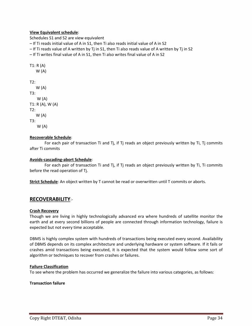
View Equivalent schedule: Schedules S1 and S2 are view equivalent – If Ti reads initial value of A in S1, then Ti also reads initial value of A in S2 – If Ti reads value of A written by Tj in S1, then Ti also reads value of A written by Tj in S2 – If Ti writes final value of A in S1, then Ti also writes final value of A in S2 T1: R (A) W (A) T2: W (A) T3: W (A) T1: R (A), W (A) T2: W (A) T3: W (A) Recoverable Schedule: For each pair of transaction Ti and Tj, if Tj reads an object previously written by Ti, Tj commits after Ti commits Avoids-cascading-abort Schedule: For each pair of transaction Ti and Tj, if Tj reads an object previously written by Ti, Ti commits before the read operation of Tj. Strict Schedule: An object written by T cannot be read or overwritten until T commits or aborts. RECOVERABILITY:- Crash Recovery Though we are living in highly technologically advanced era where hundreds of satellite monitor the earth and at every second billions of people are connected through information technology, failure is expected but not every time acceptable.
DBMS is highly complex system with hundreds of transactions being executed every second. Availability of DBMS depends on its complex architecture and underlying hardware or system software. If it fails or crashes amid transactions being executed, it is expected that the system would follow some sort of algorithm or techniques to recover from crashes or failures.
Failure Classification To see where the problem has occurred we generalize the failure into various categories, as follows: Transaction failure
Copy Right DTE&T, Odisha Page 35
When a transaction is failed to execute or it reaches a point after which it cannot be completed successfully it has to abort. This is called transaction failure. Where only few transaction or process are hurt.
Reason for transaction failure could be:
• Logical errors: where a transaction cannot complete because of it has some code error or any internal error condition
• System errors: where the database system itself terminates an active transaction because DBMS is not able to execute it or it has to stop because of some system condition. For example, in case of deadlock or resource unavailability systems aborts an active transaction.
System crash There are problems, which are external to the system, which may cause the system to stop abruptly and cause the system to crash. For example interruptions in power supply failure of underlying hardware or software failure. Examples may include operating system errors. Disk failure: In early days of technology evolution, it was a common problem where hard disk drives or storage drives used to fail frequently. Disk failures include formation of bad sectors, unreachability to the disk, disk head crash or any other failure, which destroys all or part of disk storage Storage Structure We have already described storage system here. In brief, the storage structure can be divided in various categories:
• Volatile storage: As name suggests, this storage does not survive system crashes and mostly placed much closed to CPU by embedding them onto the chipset itself for examples: main memory, cache memory. They are fast but can store a small amount of information.
• Nonvolatile storage: These memories are made to survive system crashes. They are huge in data storage capacity but slower in accessibility. Examples may include, hard disks, magnetic tapes, flash memory, non-volatile (battery backed up) RAM.
Recovery and Atomicity When a system crashes, it many have several transactions being executed and various files opened for them to modifying data items. As we know that transactions are made of various operations, which are atomic in nature. But according to ACID properties of DBMS, atomicity of transactions as a whole must be maintained that is, either all operations are executed or none.
When DBMS recovers from a crash it should maintain the following:
• It should check the states of all transactions, which were being executed. • A transaction may be in the middle of some operation; DBMS must ensure the atomicity of
transaction in this case. • It should check whether the transaction can be completed now or needs to be rolled back.

Copy Right DTE&T, Odisha Page 36
• No transactions would be allowed to leave DBMS in inconsistent state.
There are two types of techniques, which can help DBMS in recovering as well as maintaining the atomicity of transaction:
• Maintaining the logs of each transaction, and writing them onto some stable storage before actually modifying the database.
• Maintaining shadow paging, where the changes are are done on a volatile memory and later the actual database is updated.
Log-Based Recovery
Log is a sequence of records, which maintains the records of actions performed by a transaction. It is important that the logs are written prior to actual modification and stored on a stable storage media, which is failsafe.
Log based recovery works as follows:
• The log file is kept on stable storage media
• When a transaction enters the system and starts execution, it writes a log about it <Tn, Start>
• When the transaction modifies an item X, it write logs as <Tn, X, V1, V2>
• It reads Tn has changed the value of X, from V1 to V2.
• When transaction finishes, it logs: <Tn, commit>
Database can be modified using two approaches:
1. Deferred database modification: All logs are written on to the stable storage and database is updated when transaction commits.
2. Immediate database modification: Each log follows an actual database modification. That is, database is modified immediately after every operation.
Recovery with concurrent transactions
When more than one transactions are being executed in parallel, the logs are interleaved. At the time of recovery it would become hard for recovery system to backtrack all logs, and then start recovering. To ease this situation most modern DBMS use the concept of 'checkpoints'.
Checkpoint
Keeping and maintaining logs in real time and in real environment may fill out all the memory space available in the system. At time passes log file may be too big to be handled at all. Checkpoint is a mechanism where all the previous logs are removed from the system and stored permanently in storage disk. Checkpoint declares a point before which the DBMS was in consistent state and all the transactions were committed.

Copy Right DTE&T, Odisha Page 37
Recovery
When system with concurrent transaction crashes and recovers, it does behave in the following manner:
[Image: Recovery with concurrent transactions]
• The recovery system reads the logs backwards from the end to the last Checkpoint. • It maintains two lists, undo-list and redo-list. • If the recovery system sees a log with <Tn, Start> and <Tn, Commit> or just <Tn, Commit>, it puts
the transaction in redo-list. • If the recovery system sees a log with <Tn, Start> but no commit or abort log found, it puts the
transaction in undo-list.
All transactions in undo-list are then undone and their logs are removed. All transaction in redo-list, their previous logs are removed and then redone again and log saved.
Copy Right DTE&T, Odisha Page 38
CHAPTER-7
CONCURRENCY CONTROL CONCEPTS 7.1 Concurrency Control concepts:- If all schedules in a concurrent environment are restricted to serializable schedules, the result obtained will be consistent with some serial execution of transactions and will be considered correct. However using only serial schedules unnecessarily limits the degree of concurrency. Furthermore, testing for serializability of a schedule is not only computationally expensive but it is an after the fact technique and impractical. Thus concurrency control scheme is applied in a concurrent database environment to ensure that the schedules produced by concurrent transactions are serializable. The most frequently used schemes are locking and time stamp based order.
7.2 Lock Based Protocol:- A lock is nothing but a mechanism that tells the DBMS whether a particular data item is being
used by any transaction for read/write purpose. Since there are two types of operations, i.e. read and write, whose basic nature are different, the locks for read and write operation may behave differently.
Read operation performed by different transactions on the same data item poses less of a challenge. The value of the data item, if constant, can be read by any number of transactions at any given time.
Write operation is something different. When a transaction writes some value into a data item, the content of that data item remains in an inconsistent state, starting from the moment when the writing operation begins up to the moment the writing operation is over. If we allow any other transaction to read/write the value of the data item during the write operation, those transaction will read an inconsistent value or overwrite the value being written by the first transaction. In both the cases anomalies will creep into the database.
The simple rule for locking can be derived from here. If a transaction is reading the content of a sharable data item, then any number of other processes can be allowed to read the content of the same data item. But if any transaction is writing into a sharable data item, then no other transaction will be allowed to read or write that same data item.
Depending upon the rules we have found, we can classify the locks into two types. Shared Lock: A transaction may acquire shared lock on a data item in order to read its content. The lock is shared in the sense that any other transaction can acquire the shared lock on that same data item for reading purpose. Exclusive Lock: A transaction may acquire exclusive lock on a data item in order to both read/write into it. The lock is excusive in the sense that no other transaction can acquire any kind of lock (either shared or exclusive) on that same data item.
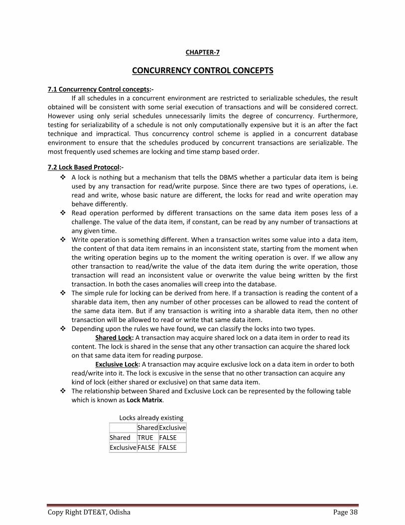
The relationship between Shared and Exclusive Lock can be represented by the following table which is known as Lock Matrix. Locks already existing
Shared Exclusive Shared TRUE FALSE Exclusive FALSE FALSE
Copy Right DTE&T, Odisha Page 39
How Should Lock be used:- In a transaction, a data item which we want to read/write should first be locked before the read/write is done. After the operation is over, the transaction should then unlock the data item so that other transaction can lock that same data item for their respective usage. For example we have a transaction to deposit Rs 100/- from account A to account B. The transaction should now be written as: Lock-X (A); (Exclusive Lock, we want to both read A’s value and modify it) Read A; A = A – 100; Write A; Unlock (A); (Unlocking A after the modification is done) Lock-X (B); (Exclusive Lock, we want to both read B’s value and modify it) Read B; B = B + 100; Write B; Unlock (B); (Unlocking B after the modification is done)
And the transaction that deposits 10% amount of account A to account C should now be written as:
Lock-S (A); (Shared Lock, we only want to read A’s value) Read A; Temp = A * 0.1; Unlock (A); (Unlocking A) Lock-X (C); (Exclusive Lock, we want to both read C’s value and modify it) Read C; C = C + Temp; Write C; Unlock (C); (Unlocking C after the modification is done)
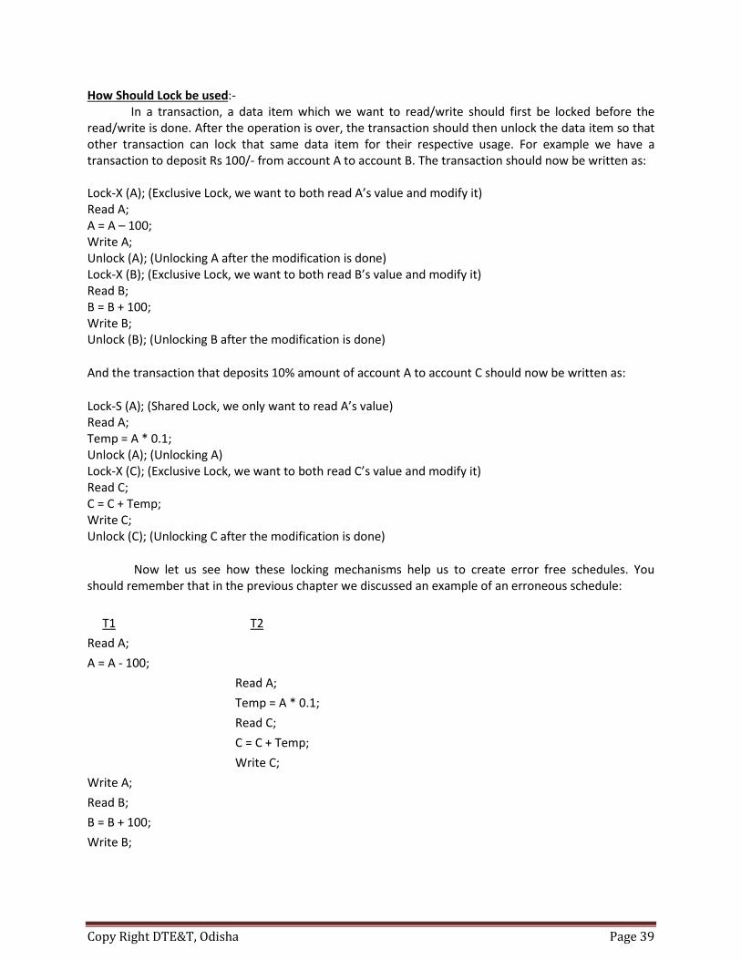
Now let us see how these locking mechanisms help us to create error free schedules. You should remember that in the previous chapter we discussed an example of an erroneous schedule:
T1 T2 Read A; A = A - 100; Read A; Temp = A * 0.1; Read C; C = C + Temp; Write C; Write A; Read B; B = B + 100; Write B;

Copy Right DTE&T, Odisha Page 40
We detected the error based on common sense only that the Context Switching is being performed before the new value has been updated in A. T2 reads the old value of A, and thus deposits a wrong amount in C. Had we used the locking mechanism, this error could never have occurred. Let us rewrite the schedule using the locks.
T1 T2 Lock-X (A) Read A; A = A - 100; Write A; Lock-S (A) Read A; Temp = A * 0.1; Unlock (A) Lock-X(C) Read C; C = C + Temp; Write C; Unlock (C) Write A; Unlock (A) Lock-X (B) Read B; B = B + 100; Write B; Unlock (B)
We cannot prepare a schedule like the above even if we like, provided that we use the locks in the transactions. See the first statement in T2 that attempts to acquire a lock on A. This would be impossible because T1 has not released the excusive lock on A, and T2 just cannot get the shared lock it wants on A. It must wait until the exclusive lock on A is released by T1, and can begin its execution only after that. So the proper schedule would look like the following:

Copy Right DTE&T, Odisha Page 41
T1 T2 Lock-X (A) Read A;
A = A - 100;
Write A;
Unlock (A)
Lock-S (A)
Read A;
Temp = A * 0.1;
Unlock (A)
Lock-X(C)
Read C;
C = C + Temp;
Write C;
Unlock (C)
Lock-X (B)
Read B;
B = B + 100;
Write B;
Unlock (B)
And this automatically becomes a very correct schedule. We need not apply any manual effort to detect or correct the errors that may creep into the schedule if locks are not used in them.
Two Phase Locking Protocol:- The use of locks has helped us to create neat and clean concurrent schedule. The Two Phase
Locking Protocol defines the rules of how to acquire the locks on a data item and how to release the locks.
The Two Phase Locking Protocol assumes that a transaction can only be in one of two phases. Growing Phase: In this phase the transaction can only acquire locks, but cannot release any lock. The transaction enters the growing phase as soon as it acquires the first lock it wants. From now on it has no option but to keep acquiring all the locks it would need. It cannot release any lock at this phase even if it has finished working with a locked data item. Ultimately the
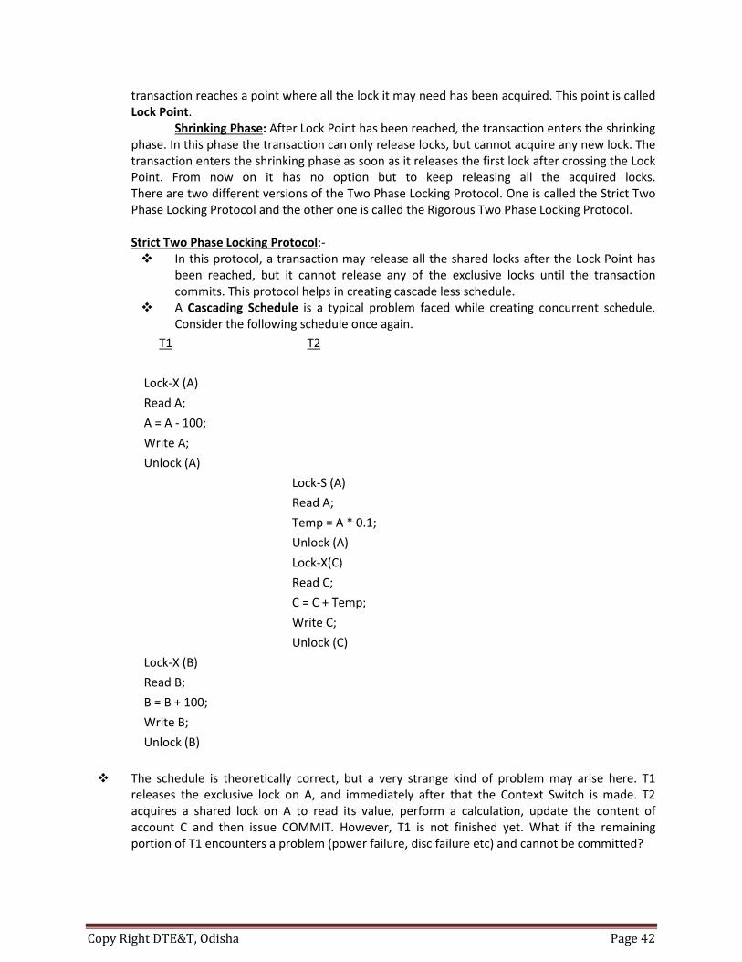
Copy Right DTE&T, Odisha Page 42
transaction reaches a point where all the lock it may need has been acquired. This point is called Lock Point. Shrinking Phase: After Lock Point has been reached, the transaction enters the shrinking phase. In this phase the transaction can only release locks, but cannot acquire any new lock. The transaction enters the shrinking phase as soon as it releases the first lock after crossing the Lock Point. From now on it has no option but to keep releasing all the acquired locks. There are two different versions of the Two Phase Locking Protocol. One is called the Strict Two Phase Locking Protocol and the other one is called the Rigorous Two Phase Locking Protocol. Strict Two Phase Locking Protocol:- In this protocol, a transaction may release all the shared locks after the Lock Point has
been reached, but it cannot release any of the exclusive locks until the transaction commits. This protocol helps in creating cascade less schedule.
A Cascading Schedule is a typical problem faced while creating concurrent schedule. Consider the following schedule once again.
T1 T2 Lock-X (A) Read A; A = A - 100; Write A; Unlock (A) Lock-S (A) Read A; Temp = A * 0.1; Unlock (A) Lock-X(C) Read C; C = C + Temp; Write C; Unlock (C) Lock-X (B) Read B; B = B + 100; Write B; Unlock (B)
The schedule is theoretically correct, but a very strange kind of problem may arise here. T1 releases the exclusive lock on A, and immediately after that the Context Switch is made. T2 acquires a shared lock on A to read its value, perform a calculation, update the content of account C and then issue COMMIT. However, T1 is not finished yet. What if the remaining portion of T1 encounters a problem (power failure, disc failure etc) and cannot be committed?

Copy Right DTE&T, Odisha Page 43
In that case T1 should be rolled back and the old BFIM value of A should be restored. In such a case T2, which has read the updated (but not committed) value of A and calculated the value of C based on this value, must also have to be rolled back. We have to rollback T2 for no fault of T2 itself, but because we proceeded with T2 depending on a value which has not yet been committed. This phenomenon of rolling back a child transaction if the parent transaction is rolled back is called Cascading Rollback, which causes a tremendous loss of processing power and execution time.
Using Strict Two Phase Locking Protocol, Cascading Rollback can be prevented. In Strict Two Phase Locking Protocol a transaction cannot release any of its acquired exclusive locks until the transaction commits. In such a case, T1 would not release the exclusive lock on A until it finally commits, which makes it impossible for T2 to acquire the shared lock on A at a time when A’s value has not been committed. This makes it impossible for a schedule to be cascading.
Rigorous Two Phase Locking Protocol:- In Rigorous Two Phase Locking Protocol, a transaction is not allowed to release any lock (either shared or exclusive) until it commits. This means that until the transaction commits, other transaction might acquire a shared lock on a data item on which the uncommitted transaction has a shared lock; but cannot acquire any lock on a data item on which the uncommitted transaction has an exclusive lock. Timestamp Ordering Protocol:- A timestamp is a tag that can be attached to any transaction or any data item, which denotes a
specific time on which the transaction or data item had been activated in any way. We, who use computers, must all be familiar with the concepts of “Date Created” or “Last Modified” properties of files and folders. Well, timestamps are things like that.
A timestamp can be implemented in two ways. The simplest one is to directly assign the current value of the clock to the transaction or the data item. The other policy is to attach the value of a logical counter that keeps incrementing as new timestamps are required. The timestamp of a transaction denotes the time when it was first activated. The timestamp of a data item can be of the following two types: W-timestamp (Q): This means the latest time when the data item Q has been written into. R-timestamp (Q): This means the latest time when the data item Q has been read from. These two timestamps are updated each time a successful read/write operation is performed on the data item Q.
How should timestamps be used:- The timestamp ordering protocol ensures that any pair of conflicting read/write operations will be executed in their respective timestamp order. This is an alternative solution to using locks. For Read operations:
1. If TS (T) < W-timestamp (Q), then the transaction T is trying to read a value of data item Q which has already been overwritten by some other transaction. Hence the value which T wanted to read from Q does not exist there anymore, and T would be rolled back.
2. If TS (T) >= W-timestamp (Q), then the transaction T is trying to read a value of data item Q which has been written and committed by some other transaction earlier. Hence T will be allowed to read the value of Q, and the R-timestamp of Q should be updated to TS (T).

Copy Right DTE&T, Odisha Page 44
For Write operations:
Chapter 1 If TS (T) < R-timestamp (Q), then it means that the system has waited too long for transaction T to write its value, and the delay has become so great that it has allowed another transaction to read the old value of data item Q. In such a case T has lost its relevance and will be rolled back. Chapter 2 Else if TS (T) < W-timestamp (Q), then transaction T has delayed so much that the system has allowed another transaction to write into the data item Q. in such a case too, T has lost its relevance and will be rolled back. Chapter 3 Otherwise the system executes transaction T and updates the W-timestamp of Q to TS (T).
LIVE LOCK:- A live lock is similar to a deadlock, except that the states of the processes involved in the live
lock constantly change with regard to one another, none progressing. This term was defined formally at some time during the 1970s ‒ in Babich's 1979 article on program correctness. Live lock is a special case of resource starvation; the general definition only states that a specific process is not progressing.
A real-world example of live lock occurs when two people meet in a narrow corridor, and each tries to be polite by moving aside to let the other pass, but they end up swaying from side to side without making any progress because they both repeatedly move the same way at the same time.
Live lock is a risk with some algorithms that detect and recover from deadlock. If more than one process takes action, the deadlock detection algorithm can be repeatedly triggered. This can be avoided by ensuring that only one process (chosen arbitrarily or by priority) takes action.
DEAD LOCK:- A deadlock is a situation in which two or more competing actions are each waiting for the other
to finish, and thus neither ever does. In a transactional database, a deadlock happens when two processes each within its own
transaction updates two rows of information but in the opposite order. For example, process A updates row 1 then row 2 in the exact timeframe process B updates row 2 then row 1. Process A can't finish updating row 2 until process B is finished, but it cannot finish updating row 1 until process A finishes. No matter how much time is allowed to pass, this situation will never resolve itself and because of this database management systems will typically kill the transaction of the process that has done the least amount of work.
Deadlock is a common problem in multiprocessing systems, parallel computing and distributed systems, where software and hardware locks are used to handle shared resources and implement process synchronization.
In telecommunication systems, deadlocks occur mainly due to lost or corrupt signals instead of resource contention.
Example:- A simple computer-based example is as follows. Suppose a computer has three CD drives and three processes. Each of the three processes holds one of the drives. If each process now requests another drive, the three processes will be in a deadlock. Each process will be waiting for the "CD drive released" event, which can be only caused by one of the other waiting processes. Thus, it results in a circular chain.
Copy Right DTE&T, Odisha Page 45
Avoiding database deadlocks:- Application developers can eliminate all risk of en queue deadlocks by ensuring that transactions requiring multiple resources always lock them in the same order. First it highlights the fact that processes must be inside a transaction for deadlocks to happen. Note that some database systems can be configured to cascade deletes which creates an implicit transaction which then can cause deadlocks. Also some DBMS vendors offer row-level locking a type of record locking which greatly reduces the chance of deadlocks as opposed to page level locking which creates many times more locks. Second, by "multiple resources" this means more than one row in one or more tables. An example of locking in the same order would be to process all INSERTS first, all UPDATES second, and all DELETES last and within processing each of these handle all parent table changes before children table changes; and process table changes in the same order such as alphabetically or ordered by an ID or account number. Third, eliminating all risk of deadlocks is difficult to achieve as the DBMS has automatic lock escalation features that raise row level locks into page locks which can be escalated to table locks. Although the risk or chance of experiencing a deadlock will not go to zero as deadlocks tend to happen more on large, high-volume, complex systems, it can be greatly reduced and when required the software can be enhanced to retry transactions when a deadlock is detected. Fourth, deadlocks can result in data loss if the software is not developed to use transactions on every interaction with a DBMS and the data loss is difficult to locate and creates unexpected errors and problems. Deadlocks are a challenging problem to correct as they result in data loss, are difficult to isolate, create unexpected problems, and are time consuming to fix. Modifying every section of software code in a large system that access the database to always lock resources in the same order when the order is inconsistent takes significant resources and testing to implement. That and the use of the strong word "dead" in front of lock are some of the reasons why deadlocks have a "this is a big problem" reputation. 7.3 SERIALIZABILITY:- Serializability is a property of a transaction schedule (history). It relates to the isolation property
of a database transaction. Serializability of a schedule means equivalence to a serial schedule (i.e., sequential with no
transaction overlap in time) with the same transactions. It is the major criterion for the correctness of concurrent transactions' schedule, and thus supported in all general purpose database systems.
The rationale behind serializability is the following: If each transaction is correct by itself i.e. meets certain integrity conditions, then a schedule that comprises any serial execution of these transactions is correct (its transactions still meet their conditions): "Serial" means that transactions do not overlap in time and cannot interfere with each other, i.e. complete isolation between each other exists. Any order of the transactions is legitimate, if no dependencies among them exist, which is assumed. As a result, a schedule that comprises any execution (not necessarily serial) that is equivalent to any serial execution of these transactions is correct.
Schedules that are not serializable are likely to generate erroneous outcomes. Examples are with transactions that debit and credit accounts with money: If the related schedules are not

Copy Right DTE&T, Odisha Page 46
serializable, then the total sum of money may not be preserved. Money could disappear, or be generated from nowhere. It does not happen if serializability is maintained.
If any specific order between some transactions is requested by an application, then it is enforced independently of the underlying serializability mechanisms. These mechanisms are typically indifferent to any specific order, and generate some unpredictable partial order that is typically compatible with multiple serial orders of these transactions.
Two major types of serializability exist: view-serializability, and conflict-serializability. View-serializability matches the general definition of serializability given above. Conflict-serializability is a broad special case, i.e., any schedule that is conflict-serializable is also view-serializable, but not necessarily the opposite. Conflict-serializability is widely utilized because it is easier to determine and covers a substantial portion of the view-serializable schedules.
View-serializability of a schedule is defined by equivalence to a serial schedule (no overlapping transactions) with the same transactions, such that respective transactions in the two schedules read and write the same data values ("view" the same data values).
Conflict-serializability is defined by equivalence to a serial schedule (no overlapping transactions) with the same transactions, such that both schedules have the same sets of respective chronologically ordered pairs of conflicting operations (same precedence relations of respective conflicting operations).

Copy Right DTE&T, Odisha Page 47
CHAPTER-8
SECURITY AND INTEGRITY 8.1 AUTHORIZATION:- Authorization is the culmination of the administrative policies of the organization, expressed as
a set of rules that can be used to determine which user has what type of access of which portion of database. The person who is in charge of specifying the authorization is usually called the authorizer. The authorizer is distinct from DBA and usually the person who owns the data.
The authorization is usually maintained in the form of a table called an access matrix. The access matrix contains rows called subject and columns called objects. The entry in the matrix at the position corresponding to the intersection of a row and column indicate the type of access that the subject has with respect to the object. Object:- An object is something that needs protection and one of the first steps in the
authorization process is to select the objects to be used for security enforcement. Example: - a unit of data, views etc.
The objects in the access matrix represent content independent access control. However to enforce content dependent access control, some structure for conditions or access predicates are incorporated in the access matrix.
Views as objects:- Views or sub schemes can be used to enforce security. A user is allowed to access only that portion of the database defined by the user’s view. A number of users may share a view. However the user may create new views based on the views allowed. The advantage of this approach is that the number of objects accessible to a class of users and the entry for it in the authorization table is reduced to one per view. This reduces the size of authorization matrix. The disadvantage is that the entire classes of users have the same access rights. Granularity:- This is used for security enforcement. This could be a file, a record or a data item. The smaller the protected object, the finer the degree of specifying protection. However the finer granularity increases the size of the authorization matrix and overhead in enforcing security. Subject:- A subject is an active element in the security mechanism. It operates on objects. A subject is a user who is given some rights to access a data object. We can also treat a class of users or an application program as a subject. Access Types:- The access allowed to a user could be for data manipulation or control. The manipulation operations are read, insert, delete, and update. The control operations are add, drop, alter and propagate.
• Read: Allows reading only the object. • Insert: Allows inserting new occurrences of the object type. Insert access type requires
that the subject has the read access as well. However it may not allow the modification of the existing data.
• Delete: Allows deleting an existing occurrence of the object type. • Update: Allows the subject to change the value of the occurrence of the object. An
update authorization may not include a delete authorization as well.
Copy Right DTE&T, Odisha Page 48
• Add: Allows the subject to add new object types such as new relations, record and set types or record types and hierarchies.
• Drop: Allows the subject to drop or delete existing object types from the database. • Alter: Allows the subject to add new data items or attributes to an existing record type
or relation. It also allows the subject to drop existing data items or attributes from existing record types or relations.
• Propagate access control: This is an additional right that if this subject is allowed to propagate the right over the object to other subjects.
VIEWS:- Sometimes for security and other concerns, it is undesirable to have all users to see the entire
relation. It would also be beneficial if we would create useful relations for different groups of users, rather than have them all manipulate the base relations. Any relation that is not part of the physical database, i.e., a virtual relation is made available to the users is known as a view.
It is possible to create views in SQL. A relation view is virtual since no corresponding physical relation exists. A view represents a different perspective of a base relation or relations.
The result of a query operation on one or more base relations is a relation. Therefore if a user needs a particular view based on the base relations, it can be defined using a query expression. To be useful, we assign the view a name and relate it to the query expression.
Create view <view name> as <query expression> A view is a relation (virtual rather than base) and can be used in query an expression that is
queries can be written using views as a relation. Views generally are not stored, since the data in the base relations may change. The definition of a view in a create view statement is stored in the system catalog. Having been
defined, it can be used as if the view really represents a real relation. However such a virtual relation defined by a view is recomputed whenever a query refers to it.
Views or sub schemes are used to enforce security. A user is allowed access to only that portion of the database defined by the user’s view.
A number of users may share a view. However, the users may create new views based on the views allowed.
The advantage of this approach is that the number of objects accessible to a class of users and the entry for it in the authorization matrix is reduced one per view. This reduces the size of authorization matrix. The disadvantage is that the entire class of users has the same access rights. We can customize all aspects of a view, including:
The name of the view
The fields that appear in the view
The column title for each field in the view
The order of the fields in the view
The width of columns in the view, as well as the overall width of the view
The set of records that appear in the view (Filtering)
The order in which records are displayed in the view (Sorting & Grouping)
Column totals for numeric and currency fields (Totaling & Subtotaling

Copy Right DTE&T, Odisha Page 49
8.2 SECURITY CONSTRAINTS:- Security in a database involves both policies and mechanisms to protect the data and ensure
that it is not accessed, altered or deleted without proper authorization. There are four levels of defense or security constraints are generally recognized for database
security: human factors, physical security, administrative control, and security and integrity mechanisms built into operating system and DBMS. Human Factors:- At the outermost level are the human factors, which encompass the ethical, legal and
social environments. An organization depends on these to provide a certain degree of protection. Thus it is unethical for a person to obtain something by stealth and it is illegal to forcibly enter the premises of an organization and hence the computing facility containing the database.
Many countries have enacted legislation that makes it a crime to obtain unauthorized dial in access into computing system of an organization. Privacy laws also make it illegal to use information for purposes other than that for which it was collected.
An organization usually performs some type of clearance procedure for personnel who are going to be dealing with sensitive information, including that contained in a database. This clearance procedure can be a very informal one, in the form of the reliability and trust that an employee has earned in the eyes of management or the clearance procedure could be a formal one.
The authorizer is responsible for granting proper database access authorization to the user community. Assignment of authorization to a wrong class of users can result in possibly security violations.
Physical Security:- Physical security mechanisms include appropriate locks and keys and entry logs to
computing facility and terminals. Security and physical storage devices (magnetic disk packs etc.) within the organization
and when being transmitted from one location to another must be maintained. Access to the computing facility must be guarded, since an unauthorized person can make copies of files by bypassing the normal security mechanism built into the DBMS and the operating system.
Authorized terminals from which database access is allowed to have to be physically secure, otherwise unauthorized persons may be able to glean information from the database using these terminals.
User identification and passwords have to be kept confidential; otherwise unauthorized users can borrow the identification and password of a more privileged user and compromise the database.
Administrative Controls:- Administrative controls are the security and access control policies that determine what
information will be accessible to what class of users and the type of access that will be allowed to this class.
DBMS and Operating System Mechanisms:- The proper mechanisms for the identification and verification of users. Each user is
assigned an account number and a password. The operating system ensures that access to the system is denied unless the number and password are valid. In addition to the DBMS could also require a number and password before allowing the user to perform any database operations.
Copy Right DTE&T, Odisha Page 50
The protection of data and programs, both in primary and secondary memories. This is usually done by the operating system to avoid direct access to the data in primary memory or to online files.
The DBMS has the following features for providing security and integrity mechanisms to support concurrency, transaction management, audit and recovery data logging. In addition the DBMS provides mechanisms for defining the authorization of the user community and specifying semantic integrity constraints and checking.
8.4 CRYPTOGRAPHY and ENCRYPTION:- Consider the secure transmission of this message:
“Mr. Watson, can you please come here” One method of transmitting this message is to substitute a different character of the alphabet for each character in the message. If we ignore the space between words and the punctuation, and if the substitution is made by shifting each character by a different random amount then the above message can be transformed into, e.g. the following string of characters:
“xhlkunsikevoabondwinhwoajahf” Cryptography has been practiced since the days of the Roman Empire. With the increasing use
of public communication facilities to transmit data there is an increased need to make such transmissions secure. In a distributed environment, transmitting highly confidential information between geographically dispersed sites, in spite of the most stringent local security enforcement could lead to leakage.
This points to the need for the data to be encrypted before it is transmitted. At the receiving end, the received data is deciphered before it is used. The sender must know how to encrypt the data and the receiver must know how to decipher the coded message. Since the computers at both ends can be used to cipher and decipher the data, the code used for ciphering is quite complex.
The simple ciphering method used since the time of Julius Caesar called Caesar code. The one time code is a Caesar code used only once, which makes it difficult for the interceptor of the coded message to break the code since he or she does not have the opportunity to intercept more than one sample of the coded message, apply the distribution characteristics of the language and break the code.
The other advantage of the onetime code is that breaking the code of a single transmission is not very helpful in deciphering subsequent coded messages, since each message will use a different code for encryption.
However the drawback is that there must be an initial transmittal of the code that is to be used to the recipient, and for absolute unbreakability, the code has to be as long as the message that is transmitted.
A enciphering scheme developed by the U.S National Bureau of Standards(NBS) is called the Data Encryption Standard(DES). This scheme is based on the substitution of characters and rearrangement of their order and assumes the existence of secure encryption keys. It is a relatively easy means to both encipher and decipher data. The algorithm is very well known and publicized but the encryption key is kept secret, which makes it very difficult for anyone who does not know the key to decipher the message. However the drawback in this scheme is that the encryption key has to be transmitted to the recipient before a message can be transmitted. Due to this drawback an encryption technique called one-way or trapdoor functions having the following characteristics:-
Copy Right DTE&T, Odisha Page 51
1. It can change any message X into a message Y. 2. It has an inverse function that changes Y back into X. 3. Efficient algorithms can be devised to change X into Y and Y back to X. 4. If the function and the algorithm to convert from X to Y is known, then the same enciphering
and deciphering functions can be used over and over again. The last property gives the function its name: the trapdoor function, easy to drop through but hard to get out of it. The knowledge of an appropriate trapdoor function allows the use of a public key encryption scheme where both the encryption key and encryption algorithm are public and readily available. This allows anyone to send message in a coded form, however the decryption key is secret and only the rightful recipient can decipher the coded message. 8.3 INTEGRITY CONSTRAINT:- Integrity constraints ensure that any properly authorized access, alteration, deletion or insertion of the data in the database does not change the consistency and validity of the data. Database integrity involves the correctness of data; this correctness has to be preserved in the presence of concurrent operations, errors in the users operations and application programmes and failures in hardware and software. Constraints are restrictions or rules applied to a database to maintain its integrity. They are-
1. Data/Entity integrity constraint 2. Referential integrity constraint
1. Data constraint:-
It is the most common integrity constraint also known as domain integrity constraint. Domain integrity rules are simply the definition of the domains of the attributes or the value set for the data items. The value that each attribute or data item can be assigned is expressed in the form of data type, a range of values or a value from a specified set. Example: In the relation EMPLOYEE the domain of the attribute Salary may be in the range of 12000 to 300000 The domain values supplied for an operation are validated against the domain constraint. In specifying the domain constraints, null values may or may not be allowed. Thus it is usual not to allow null values for any attribute that forms part of a primary key of a relation.
2. Referential integrity constraint:- It is an implicit integrity constraint which states that, a tuple in one relation that refers to another relation must refer to an existing tuple in that relation. The referential integrity rule is explained by the foreign key between two relation schemas R1 and R2. A set of attributes Fk in relation schema R1 is a foreign key of R1 that references relation R2 if the following two rules are being satisfied.
i)The attributes in foreign key Fk have same domain as primary key attributes Pk of R2,the attributes Fk are said to be referenced or referred relation R2. ii) A value of Fk in tuple T1 of the current state R1 (r1) either occurs as a value of Pk for some tuple T2 in the current state R2 (r2) or is none. In the former case we have T1 [Fk] = T2 [Fk] and we say that the tuple T1 references or refers to the tuple T2. R1 is called the referencing relation and R2 is called referenced relation.

Copy Right DTE&T, Odisha Page 52
REFERENCE BOOKS
1. An Introduction to Database Systems By: - C.J. Date
2. DATABASE System Concepts A. Silberschatz, H.F. Korth,
3. The Database book, principles & practices, Unv. SC. Press
4. Database System concepts; Rog,Cornel; Cengage Learning
5. Data Base System; B. Desai; Galgotia Publication
Copy Right DTE&T, Odisha Page 53
Model Questions Questions Carrying Two Marks Each:-
1. What do you mean by Data Abstraction? 2. What is a Database Language? 3. What is the Role of DBA? 4. What do you mean by a Database System? 5. What is an entity? 6. What do you mean by an attribute? 7. What do you mean by a data Model? 8. What is an E-R Diagram? 9. What do you mean by a Tuple? 10. What do you mean by a Relation? 11. Explain Relational Algebra. 12. Define Selection and Projection Operations in relational algebra. 13. Define Cartesian product Operation. 14. Write down Importances of Normalization? 15. What do you mean by a Primary Key? 16. What is a Foreign Key? 17. What is a Candidate Key? 18. What is an Alternate Key? 19. What do you mean by a Query Language? 20. What are the Various Commands used in DDL? 21. What are the Various Commands used in DML? 22. What is a Structure Query Language? 23. What do you mean by Referential Integrity Constraint? 24. What is an Entity Integrity Constraint? 25. What is a Transaction? 26. What do you mean by Transaction Processing? 27. What is a Fault? 28. What is an error? 29. What do you mean by Reliability? 30. What is a Shared Lock? 31. What is an Exclusive Lock? 32. What do you mean by Dead Lock? 33. What is a View?

Copy Right DTE&T, Odisha Page 54
Questions Carrying Six Marks Each:-
1. What is the Purpose of Database Systems? 2. What are the Various Database users? 3. Explain different types of Database Languages. 4. Explain briefly the Importance of Data Dictionary. 5. What is Data Independence? Explain it. 6. What is an Attribute? Describe the Various Types of Attributes used in ER-Model. 7. What do you mean by Mapping Constraint? Explain it with Suitable Example. 8. What do you mean by Relational Algebra? Explain different types of Operations used in
database with suitable examples. 9. What is a Lossless Join? 10. What do you mean by BCNF? Explain with suitable example. 11. Write down the Syntaxes of CREATE, SELECT, UPDATE and INSERT commands used in SQL and
explain them with suitable Examples. 12. Write down briefly the Different States of a Transaction? 13. Explain the 2-Phase Locking Concept with suitable example. 14. How Recovery can be done in case of a Database System failure? 15. Discuss the Idea behind Encryption Technique?
Questions Carrying Eight Marks Each:-
1. What do you mean by Data Abstraction? Explain it with Suitable Diagram. 2. Explain E-R Model with suitable example. 3. What is a Relational data Model? Explain it briefly. 4. What are the various features of Hierarchical data Model? 5. Explain Network data model with Example. 6. Discuss the various relational algebra operations with suitable Examples. 7. Compare the First, Second and third Normal Forms. 8. What is SQL? Write down the various DDL & DML Commands used with suitable examples. 9. What is a Transaction? State the various Properties of Transaction. 10. Explain The Idea behind serializability. 11. How Concurrency can be managed in Databases? Explain it. 12. How the security is maintained in a Database?