Education, Employment and Earnings of Secondary School-Leavers in Tanzania:

Evidence from a Tracer Study*

Samer Al-Samarrai ** Barry Reilly Institute of Development Studies Poverty Research Unit at Sussex University of Sussex Department of Economics Falmer University of Sussex Brighton Falmer BN1 9RE Brighton United Kingdom BN1 9SN e-mail: alsamarrai@msbx.net United Kingdom

PRUS Working Paper no. 31

Abstract The extent of information on labour market outcomes and the earnings of educated groups in Tanzania, and Sub-Saharan Africa more generally, are limited. This is particularly so for individuals who fail to gain access to wage employment and are required to rely on exploiting self-employment opportunities. The current paper, using a recently completed tracer survey of secondary school completers, analyses the impact of education and training on individual welfare through the estimation of earnings equations. Our empirical evidence suggests that the rates of return to educational qualifications are not negligible and, at the margin, provide an investment incentive. However, we find little evidence of human capital effects in the earnings determination process in the self-employment sector. Information contained in the tracer survey allowed the introduction of controls for father’s educational background and a set of school fixed effects designed to proxy for school quality and potential labour market network effects. The analysis shows that the inclusion of these controls tends to reduce the estimated rates of return to educational qualifications. This emphasizes the potential confounding role of school quality/network effects and parental background for rate of return analysis. We would argue that a failure to control for such background variables potentially leads to an over-statement in the estimated returns to education. A comparison of our results with evidence from other countries in the region shows that despite an extremely small secondary and university education system the private rates of return to education in the Tanzanian wage employment sector are relatively low. * The data used in this survey is from wider project undertaken in four Sub-Saharan African countries funded by the United Kingdom’s Department for International Development (DfID). Faustin Mukyanuzi of HR Consult implemented the survey in Tanzania and overall findings are reported in Mukyanuzi (2003). The views expressed in this paper are entirely those of the authors and do not necessarily represent the DfID’s own policies or views. ** Corresponding author.

1

1. Introduction

Information on labour market outcomes, including the earnings of educated groups, in

Sub-Saharan Africa is limited. Government and individuals in this region invest

heavily in education and training but little is generally known about how these

investments generate rewards in the labour market. This is particularly so for

individuals who fail to gain access to wage employment and are required to rely on

exploiting self-employment opportunities. The current paper, using a recently

completed tracer survey of secondary school completers from Tanzania, analyses the

impact of education and training on individual welfare through the estimation of

earnings equations.

Earnings equations provide a convenient framework within which average private

rates of return to educational qualifications and training can be computed.1 There is a

dearth of evidence on the magnitude of these rates for wage employees in Tanzania

and almost none for individuals in self-employment. Given the increasing number of

secondary school-leavers entering self-employment this represents a substantial

lacuna in the literature. The aim of this paper is to partially fill this gap by estimating

sectoral-specific earnings equations for employees and the self-employed from a

cohort of secondary school students who completed junior secondary schooling in

Tanzania in the 1990s.

Tracer surveys of the kind used in this paper, unlike conventional labour force or

household surveys, permit the collection of additional information on parental

background and schooling quality. This allows for some important refinements to the

specification of the earnings equations. In particular, the independent role of parental

background and, inter alia, schooling quality can be explored and the extent to which

the estimated returns to the general human capital measures alter with the inclusion of

these variables investigated.

1 Card (1999) provides a detailed review of methodological and other issues germane to the estimation and interpretation of earnings equations.

2

The structure of the paper can now be outlined. In order to place our empirical

analysis in context the next section provides a brief history of the education system in

Tanzania and reviews the changes in the labour market over the 1990s. This section

also summarises some of the findings from a small number of earlier studies that have

estimated earnings equations for Tanzania. Section 3 outlines the data and describes

some of the advantages and drawbacks in estimating earnings equations using tracer

survey data. Given the recorded nature of the earnings data and potential selection

issues, section 4 outlines the econometric methodology and details how the estimated

regression models are evaluated. Section 5 reports the empirical results and section 6

offers some conclusions.

3

2. Background

In the aftermath of Tanzania’s independence in 1962 education policy focussed on

expanding access to basic education as a key component of the government’s socialist

economic and social development strategy.2 Tanzania achieved rapid success, with

enrolments in primary schools increasing four-fold during the 1970s, reaching

primary gross enrolment rates of 100 per cent by the early 1980s (MOEC BEST

1985).3 These dramatic increases in primary education access were not matched by

increases in secondary school enrolment. The access to the latter was restricted both

because of resource constraints arising from primary school expansion, and because

the Government restricted the establishment of private secondary schools in an

attempt to reduce inequality of access.4 Rising primary school enrolments with limited

secondary school expansion resulted in a decline in the proportion of primary school-

leavers progressing to secondary level. The proportion of standard VII leavers

continuing to secondary school plummeted from over one-third in 1961 to under one-

fifth in 1967, and by 1980 was only seven per cent (see Knight and Sabot (1990)).

The war with Uganda and its consequences were largely responsible for the

Tanzanian recession experienced during the late 1970s and early 1980s. The

economic downturn and the subsequent adjustment policies led to major declines in

primary school enrolment rates, which by 1990 had declined to approximately 70 per

cent. The impact was very different for secondary schooling. Parental pressure and

constrained government finances led to an easing of restrictions on private and

community schools during the 1980s (see Samoff (1987)). As a consequence,

secondary school enrolments doubled between 1984 and 1990 (MOEC BEST, various

years), largely because of increases in the number of private schools, but also through

rising numbers of community-built government schools.

2 At the time of independence secondary and tertiary education were strengthened to provide skilled manpower for public administration. 3 The primary gross enrolment rate for Tanzania is defined as total primary school enrolment divided by the seven to 13 year old population. 4 Parents demanding greater secondary school access tended to be concentrated in particular areas of the country and allowing private schools to be established in these areas would have led to geographical inequities in secondary school provision. See Samoff (1987) for a detailed account of these issues.

4

Despite large absolute increases in the secondary school system through the 1980s

and 1990s, enrolment rates remained amongst the lowest in the world and compared

unfavourably with other countries in the region (six per cent in Tanzania as compared

to 27 per cent in sub-Saharan Africa in 2000 (UNESCO 2003)). An even smaller

proportion is selected into senior secondary schooling. For instance, in 1999 only 27

per cent of junior secondary school graduates went onto the senior level (MOEC

BEST 2000).5 Progression from senior secondary school to university is also severely

restricted and while tertiary enrolments more than doubled over the 1990s, less than

one per cent of the school aged population received tertiary education. As Table 1

shows, the Tanzanian education system is highly selective, with large numbers of

completers at each level failing to continue with their education. Only two per cent of

the population aged 25 or over had completed the full six years of secondary

education. It is also interesting to note that in a nationally representative survey

undertaken in 1993, based on approximately 5,000 households and 30,000

individuals, not a single respondent had completed a university degree.

[Table 1]

Labour force surveys undertaken in 1991 and 2000 provide some indication of the

nature of the labour market that increasing numbers of secondary school completers

and university graduates entered during the course of that decade. The economically

active population in Tanzania almost doubled during the 1990s, although this rise was

not matched by a growth in wage employment opportunities. By the end of the 1990s

the share of wage employment in the economically active labour force had declined

from eight to six per cent (Planning Commission 1993 and 2000). The majority of the

increase in the economically active population was absorbed into the traditional

agricultural sector, with some increases in non-traditional agricultural self-

employment. Based on this limited evidence it seems likely that over the 1990s the

rising number of secondary school leavers and university graduates entering the

labour force exceeded the growth in wage employment opportunities. It also appears

5 The secondary school system in Tanzania is split into junior secondary (Forms I-IV) and senior secondary (Forms V-VI).

5

that a greater number of educated groups became self-employed during this period.

The data from the survey used in this paper are consistent with this interpretation of

the trends. A comparison of the 1990 and 1995 cohorts of secondary school

completers reveals, after the same number of months in the labour force, a greater

proportion of the earlier cohort in wage employment (see Al-Samarrai and Bennell

(2003)).

The changes in the demand for educated individuals and the numbers entering the

labour force after completing their education clearly impacts on the private rate of

return to education secured in the labour market. Table 2 summarises the findings of

studies that have estimated private rates of return to educational qualifications in the

Tanzanian formal sector over the last 30 years. The returns to secondary exceed those

to primary in Tanzania and this possibly reflects the high proportion of the labour

force with primary education and the very limited numbers with secondary education.

In addition, university rates of return are significantly higher than those accruing to

secondary education. Therefore, the education system, given its selective nature,

appears to give rise to high premia for individuals who gained access to secondary

and university education.

[Table 2]

This pattern of returns to education differs from those observed elsewhere in sub-

Saharan Africa and other developing countries. Private rates of return to primary,

secondary and university education in the region tend to be much higher than those

reported in table 2. Moreover, a recent review revealed higher returns to primary than

to secondary education in sub-Saharan Africa (see Psacharopoulos and Patrinos

(2002)).6 Table 2 also shows that rates of return to university qualifications are much

higher than those obtained in the primary or secondary sectors. While the most recent

review suggests that primary returns are higher than university returns, five out of the

6 In periodic reviews of rates of return studies across the world Psacharopoulos has provided regionally aggregated rates of return to different levels of education. These have consistently shown that primary education has the highest private returns followed by university and then secondary education. However, there has been substantial debate around the quality of data used in these regional aggregates as well as the time period covered. Bennell (1996) shows that the aggregated rates of return to secondary exceed primary for sub-Saharan Africa if poor quality studies are excluded.

6

nine studies reviewed for sub-Saharan Africa showed a similar pattern to table 2,

whereas the remaining four found higher rates for primary and sometimes secondary

(see Table A1 Psacharopoulos and Patrinos (2002)).7

The rates of return reported in table 2 are for formal sector workers only and give no

indication of the rates of return in other sectors. But as wage employees represent a

very small proportion of the total labour force, this does not provide a complete

portrait of the returns to education. One objective of the current paper is to explore

the rates of return to secondary and university education in both wage and self-

employment sectors. Based on data from the sample of secondary school completers

used in this paper, table 3 shows that income from self-employment is significantly

lower than earnings from wage employment for this group of completers.

[Table 3]

7 In Psacharopoulos and Patrinos (2002) full method rates of returns are used while our table 2 reports estimated rates of return from extended earnings functions.

7

3. Data

The data used in this paper are drawn from a tracer survey conducted in Tanzania

during 2001.8 Tracer surveys are designed to find a group of individuals who have

shared a specific type of training or educational background. Tracer surveys are thus

able to explore the impact of a common training or educational background on

specific labour market outcomes.

In exploring the link between education and labour market outcomes, tracer surveys

have some advantages over conventional labour force or household surveys. The

school that an individual attends may influence the type of work or training pursued

and the income earned after school completion. This may be particularly important in

very small systems such as the secondary education system of Tanzania. In general,

labour force surveys do not collect information on school characteristics or academic

achievement. Many of these types of studies focus only on the years or quantity of

schooling acquired. By tracing individuals through the schools they originally

attended, tracer surveys allow information on school characteristics to be collected,

which may be helpful in analysing the impact of education on labour market

outcomes and earnings.

A criticism of studies that explore the impact of education on earnings in developing

countries is that they only tend to look at the impact of education on formal sector

wages.9 Focusing solely on wage employment is likely to distort the impact of

education on future earnings. Many studies also fail to take account of the potential

sample selection bias arising from the division of the labour force into different

activities, and in particular into wage and self-employment. As tracer surveys collect

information on a cohort of students, it is possible both to estimate separate wage

equations for wage and self-employment and correct for the potential sample selection

bias arising from the initial labour market sectoral choice. 8 The Tanzania secondary school tracer survey analysed in this paper formed part of a larger project conducted for secondary school leavers and university graduates in Malawi, Tanzania, Uganda and Zimbabwe. For details of the wider research findings see Al-Samarrai and Bennell (2003). 9 For a review of the estimation issues involved see Bennell (1996) and Glewwe (2002).

8

It should be noted, however, that estimating earnings equations using tracer survey

data provides limited information on the age-earnings profile since in such surveys

individuals tend to be clustered around certain ages determined by school starting age

and individual progression through the school system. In addition, tracer surveys only

include information on a cohort of individuals that has achieved a certain level of

education and/or training and therefore contains no information on those who have

lower levels of education or no formal education. For example, the focus of the tracer

surveys in this study is on secondary education. Therefore, all individuals in the

analysis have attained at least junior secondary education.

Another potential drawback of tracer surveys is that they suffer from sample selection

issues that potentially bias the analysis towards individuals that are more easily

traced. For example, some tracer surveys do not sample individuals from a complete

list (sample frame) of individuals with the same training. Instead they trace

individuals by visiting major enterprises or organisations where individuals with the

specified training are likely to work. All those that were not able to get work in these

organisations are excluded, potentially biasing any analysis of the group as a whole.

In cases where tracer surveys do use a sample frame to randomly select individuals

they only manage to trace a small proportion of the sampled individuals. Again, low

response rates may be taken to infer that selection bias is likely to be a serious

problem.

The tracer survey for this study was carefully designed to avoid the type of problems

commonly associated with surveys of this kind. The tracer survey aimed to locate a

specific group of secondary school-leavers that completed the first four years of

secondary schooling in Tanzania. The sample of secondary school-leavers was

selected from ten average performing secondary schools: five located in Dar es

Salaam and five in Dodoma.10 The sample frame consisted of all students in these

schools who completed their junior secondary schooling in 1990 or 1995. A random

10 As mentioned in the previous section secondary school access was very low during the 1990s and the 10 sampled schools represents about 2 per cent of the total number of secondary schools in Tanzania at this time.

9

sample of 50 completers from each of the two years were randomly selected from

each school to comprise a total of 1000 junior secondary school completers.

Once initial lists of sampled students were collated, research teams attempted to trace

each individual’s current location. Tracing selected individuals began at the schools,

where staff members and school records provided some information. The research

teams then interviewed and completed questionnaires on all sampled respondents

living in the vicinity of the schools. In addition to interviewing these respondents the

research teams asked about the current whereabouts of sampled classmates, where the

school was unable to provide sufficiently accurate information to locate them. The

research teams also interviewed parents and other household members of sampled

students who were living elsewhere, to obtain information on their current location as

well as to collect basic information on the individual in question. Asking family

members and classmates about the location of sampled students proved to be an

extremely productive tracing technique. Once the research teams completed the work

in the vicinity of the sampled schools, researchers were sent to interview respondents

in other cities and locations with high concentrations of traced completers. In cases

where traced respondents lived in remote areas a questionnaire was sent to them for

completion.11

Table 3 shows the tracer survey response rate to be extremely high, with 97 per cent

of respondents being traced and their information collected. This compares favourably

with other tracer surveys conducted in developing countries (see for example, Bennell

and Ncube (1993, 1994), Kaijage (2000), Narman (1992), Mayanja and Nakayiwa

(1997)) and suggests that sample selection problems may be considerably reduced in

our case. The main source of the information collected was the traced respondent, and

in the majority of cases this was through ‘face-to-face’ interviews. In 50 cases basic

information on the respondents was collected from the individual’s parents.

A questionnaire was completed for each respondent and was designed to elicit

information on personal background, further education, training and employment

11 This was rarely done through the postal service but through intermediaries living near the sampled individual.

10

history, current activity and income. It should be noted that no information was

collected for respondents who were overseas (or deceased) at the time of the survey,

and these respondents are thus excluded from the present study. Of the remaining 940

respondents, the necessary information was available for 923 to be included in the

analysis.12 Table A1 in the appendix provides a full description of the variables used

in the analysis and table A2 reports some summary descriptive statistics.

12 Of these, 402 were in wage employment and 214 were self-employed. The remainder were either unemployed or undertaking training.

11

4. Methodology

The primary objectives of our research are served by the estimation of earnings

equations for the sample of traced Tanzanians. In order to elicit responses that are

less prone to measurement error interviewees were asked where their gross monthly

earnings were located within a number of mutually exclusive categories. The

intervals used for the sampled employees in our case commence at 0 to 50,000

shillings and rise by amounts of 50,000 for the next five intervals.13 The penultimate

interval is 300,000 to 400,000, and the final interval is open-ended and captures those

individuals with earnings greater than 400,000 Tanzanian shillings. There are thus

eight coded intervals for the case of employees. A corresponding exercise was

conducted for the self-employed but the intervals used are different. They are ten in

number and, in contrast to the wage employees, relate to a bi-annual earnings

measure.14 However, the econometric methodology outlined is identical for both

cases and for convenience the exposition is cast in terms of the earnings categories for

the employees.

The data on the dependent variables are ordinal in nature but interval coded. An

appropriate econometric procedure is required to deal with the nature of these coded

responses. There are two possible procedures that could be exploited here. The

cruder of the two involves setting earnings to the mid-point of the relevant intervals

and applying the ordinary least squares (OLS) procedure. A more desirable approach,

however, is to follow Stewart (1983) and use an appropriate likelihood function for

the application at hand. The likelihood function is a modification of that used in the

estimation of the standard ordered probit model and replaces the unknown threshold

values by the set of known thresholds that delineate the intervals. The responses on

the dependent variable are grouped. In the early literature this type of model was

referred to as a grouped dependent variable model but more recently the term interval

regression model has been used to describe it.

13 At the time of the survey there were 876 Shillings to the US dollar. 14 The precise intervals for the self-employed are described in the notes to table 5.

12

In order to understand how the model is implemented, responses are coded 1,2,…..,8

to capture the eight distinct earnings categories in our application for employees.15

Let yi denote the observable ordinal variable coded in this way and let y*i denote an

underlying variable that captures the earnings of the ith individual. This can be

expressed as a linear function of a vector of explanatory variables (xi) using the

following relationship:

�x'i

*iy = + ui where ui ~ N(0, σ2) [1]

It is assumed that y*i is related to the observable ordinal variable yi as follows:

yi = 1 if a0 < y*i < a1

yi = 2 if a1 ≤ y*i < a2

yi = 3 if a2 ≤ y*i < a3

yi = 4 if a3 ≤ y*i < a4

yi = 5 if a4 ≤ y*i < a5

yi = 6 if a5 ≤ y*i < a6

yi = 7 if a6 ≤ y*i < a7

yi = 8 if a7 ≤ y*i < +∞

where the aj for j=1,…8 denote the interval boundaries. Following Stewart (1983), we

treat the first and the last intervals as open-ended in this case so for j=0, Φ(aj) = Φ(–

∞) = 0 and for j=8, Φ(aj) = Φ(+∞) = 1, where Φ(·) denotes the cumulative distribution

function for the standard normal.16

The exact knowledge of the thresholds allows the likelihood function to be specified

in a fairly straightforward manner. The variable y*i is best interpreted not as a latent

measure but one with a quantitative interpretation. In implementing the procedure the

standard normal assumption conventionally invoked for the ordered probit model is

15 The focus on the employees is expositional and the j (or sectoral subscript) is ignored for convenience. 16 In the case of the self-employed sample, there are ten categories and thus nine known threshold values.

13

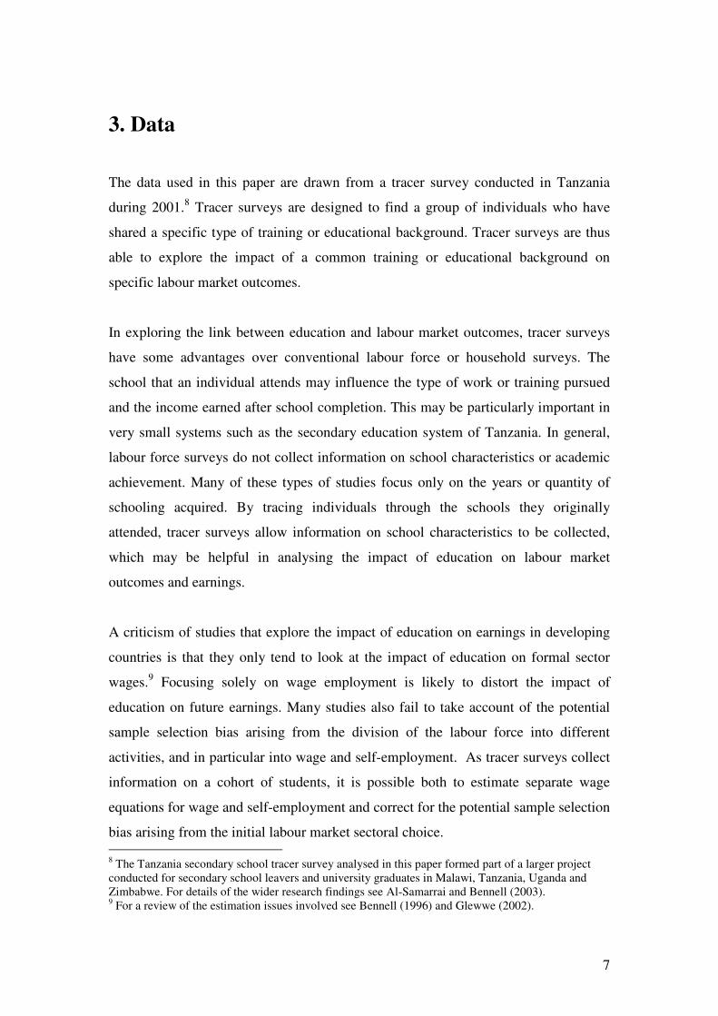
replaced by the assumption that y*i | xi ~ N( �x'

i ,σ2). This then allows specification of

the log likelihood function as follows:17

L = �=

J

0j�

=

jyi

loge[Φ(σ

− �x'ija ) – Φ(

σ− �x'i1-ja

)] [2]

where the first summation operator sums across individuals within the given j

category and loge(·) denotes the natural logarithmic operator. The maximum

likelihood procedure involves the estimation of the ββββ parameter vector and the

ancillary standard error parameter σ. Given that the introduction of the known

thresholds fixes the scale of the dependent variable, the estimated coefficients are

amenable to a direct and more intuitive OLS-type interpretation. The estimates

contained in the ββββ parameter vector are interpretable on the assumption that we have

actually observed the y*i outcome for each of the i individuals in the sample.

It is important to evaluate our empirical models in regard to certain key econometric

assumptions. The adequacy of the estimated models is assessed using the efficient

score tests suggested by Chesher and Irish (1987). These tests require computation of

the models’ pseudo-residuals. In general terms, the pseudo-residual for the ith

individual is defined for the interval regression model as:

ui = )]()([

)()('i'i

'i'i

1-jj

j1-j

aa

aa

σ−Φ−

σ−Φσ

σ−φ−

σ−φ

�x�x

�x�x [3]

where φ(·) denotes probability density function operator for the standard normal. 18

17 The only difference between this log-likelihood function and that of the ordered probit is that in our case the threshold values are known and σ is estimated and not constrained to unity. The exact knowledge of the thresholds allows identification of the scale of the dependent variable and estimation of σ. 18 The pseudo-residuals can be obtained by differentiating the log-likelihood expression in [2] with respect to the constant term implicit in the x vector.

14

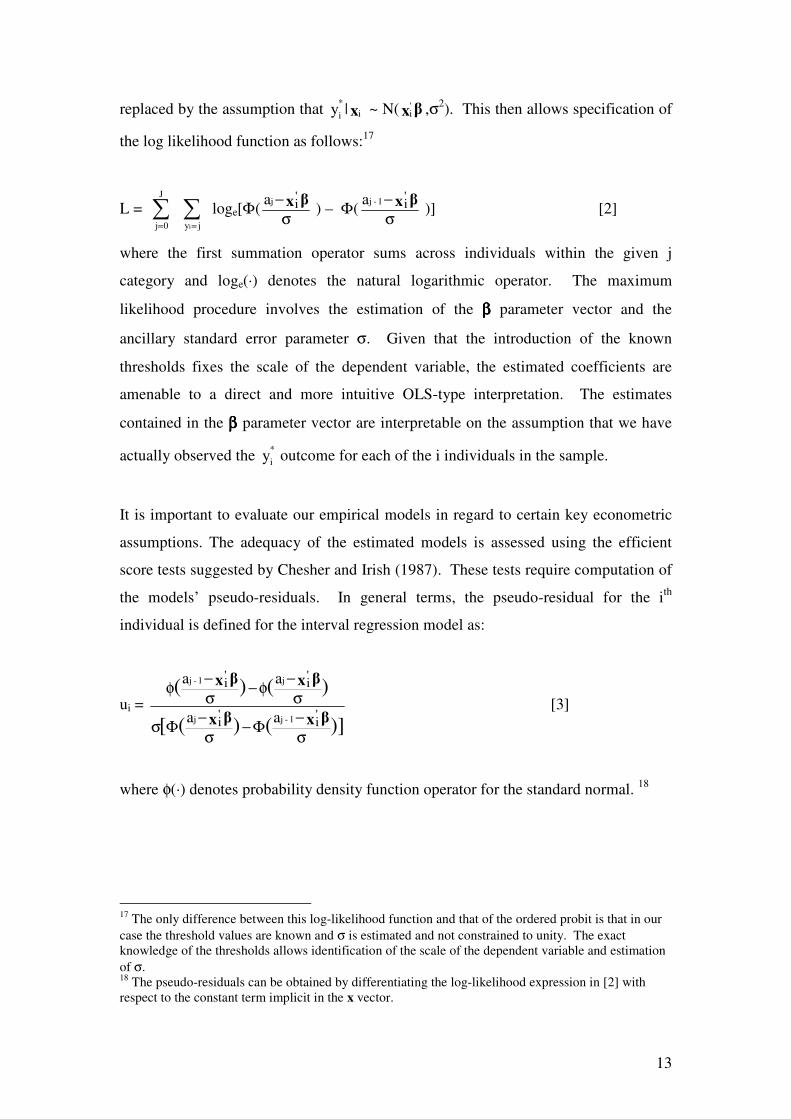
These pseudo-residuals are then used in computation of the score tests. In order to

implement these tests we also need the score contribution for the σ parameter. This is

obtained as:

σ_scorei =

)]()([

)()('i'i

'i'i'i'i

1-jj2

jj

1-j1-j

aa

a)(a

a)(a

σ−Φ−

σ−Φσ

σ−φ−−

σ−φ−

�x�x

�x�x

�x�x

[4]

The score tests take the form i′′′′R(R′′′′R)-1R′′′′i. In this case, i is an n×1 ‘summer’ vector

of ones, and R is an n×q matrix of score contributions computed for each of the k

parameters from the original specification and the k+1,….q parameters that capture

the form of the alternative hypothesis, assumed zero under the null. A typical row

element for R is given by:

R = [ui, uix1i,……., uixki,σ_scorei, Q1i,….Qqi] [5]

The Q1i,….Qqi measures capture the alternatives under test. If the Q1i,….Qqi terms

were excluded from R the score test would be zero by construction. The introduction

of the Q1i,….Qqi terms induce a departure from zero and the purpose of the test

statistic is to determine whether the difference from zero is statistically significant or

not.

The score tests focus on three key properties of the econometric specifications. These

are (i) pseudo-functional form, (ii) homoscedasticity, and (iii) normality. The pseudo-

functional form tests are based on the RESET principle conventionally applied to the

linear regression model (see Ramsey (1969)).19 The test uses the predicted

standardised index raised to the second, third and fourth powers as auxiliary measures

to capture model mis-specification. Thus, Q1i, Q2i, Q3i are constructed by interacting

the pseudo-residuals from the interval regression model (ui) with the model’s

predicted standardised index )('i

j

σ�x where j=2,3,4. There are thus three degrees of

19 Peters (2000) examines the power of the RESET for a number of microeconometric models.

15

freedom for this test. In regard to the homoscedasticity test, the set of explanatory

variables included in the earnings specifications provide the basis for the alternative

heteroscedastic relationship. The Q1i to Qki terms are constructed by interacting the

σ_scorei term with the x1i to xki explanatory variables from the regression model. The

reported degrees of freedom for this test are thus equal to the number of explanatory

variables in the original specification. The normality test examines departures from

skewness and kurtosis and the Q1i and Q2i measures are constructed in this case by

interacting the pseudo-residuals with expressions for the third and fourth moment

residuals (see Chesher and Irish (1987) for more details). The number of degrees of

freedom in this case is two.

The resultant test statistics are all distributed as chi-squared with p = q – k degrees of

freedom. The test represents the outer-product gradient (OPG) form of the score (or

Lagrange Multiplier) test. Orme (1990) has questioned the use of OPG-based tests

and, using Monte Carlo simulations, demonstrated their poor finite sample properties

in the context of the binary probit model. Orme’s findings suggest that efficient score

tests constructed using the OPG covariance matrix tended to reject the correct null

hypothesis far too frequently. Given the modest sample sizes we use here this may be

viewed as something of a concern. Even if the simulation findings extend to the

interval regression models used here, though, the implication in using these tests is

that we are actually setting the estimated models a more stringent set of criteria to

pass. We take the view that it is more desirable to be transparent about the test

findings and report rather than ignore them. 20

In circumstances where the homoscedasticity and/or normality assumptions are

violated, the variance-covariance matrix is corrected using the Huber (1967)

‘sandwich’ estimator, which provides an appropriate asymptotic matrix for an

estimator that is biased in an unknown direction.21 This is defined as:

Var-Cov(∧� ) = [I(

∧� )]-1( x'

i u2i xi) [I(

∧� )]-1 [6]

20 The estimation reported in this paper was undertaken using the LIMDEP 7.0 software package. 21 However, see Greene (2000, pp.823-824) for some cautionary comments about its use and validity.

16

where I(∧� ) is the information matrix for the

∧� vector computed at the maximum

likelihood estimates.

Given that we are interested in estimating an earnings equation within the established

Mincerian tradition, the thresholds used in the log-likelihood function [2] are based on

the natural logarithms of the reported thresholds. Thus, in the context of the

employee specification, a1= loge(50,000) and a7= loge(400,000), and so forth.22

Finally, there is potential for selection bias in the estimated earnings equations. The

samples of employees and the self-employed may not represent a random drawing

from the population of school-leavers.23 As a consequence, the estimated coefficients

for the returns to education and other characteristics may be potentially biased. In

order to address this problem we use the procedure developed by Lee (1983), which

provides a more general approach to the correction of selectivity bias than that

originally offered by Heckman (1979). The procedure is also two-step but exploits

estimates from a multinomial logit model (MNL) rather than a probit to construct the

set of selection correction terms. We first estimate the reduced form MNL for the

j=1,...,k categories and obtain the parameter estimates γj. In our application k=4 with

employees, the self-employed, those in training and the unemployed providing the

four mutually exclusive categories. The predicted probabilities for each individual

i=1,....,N for each category j are then computed and defined as Pi1,Pi2,....Pi4. The

‘normits’ or standardized z values for each individual for each category j using the

inverse standard normal operator are then computed. Thus: zi1 = Φ-1(Pi1), zi2 = Φ-

1(Pi2),........ zi4 = Φ-1(Pi4) for all i=1,.....N. Finally, for each j category we construct the

following correction term:

ij

ijij

P)z(φ=λ for i=1,2,.......N and j=1,2,...k [7]

22 See the notes to table 1 for the full set of intervals used in the case of the employees. 23 In fact there is another potential source for selection bias in the estimation of our wage equations given that our sample is conditioned on secondary school-leavers. It thus excludes those with primary-level or no education. Given the positive relationship between earnings and education, the underlying wage distribution may be truncated at the bottom end and there may be potential for an upward bias in our estimated educational returns as a consequence. In contrast to employment selection, there is nothing that can be feasibly done to address this selection problem given existing data constraints.

17

where φ(·) denotes the probability density function for the standard normal. These selection terms are analogous to those computed using the more conventional

two-step Heckman procedure. The relevant selection terms are then added to the xi

vector in the interval regression models. Instruments are required to identify the

parameters of the selection effects in the earnings equation. These need to be chosen

such that they shift the probability of sectoral attachment but not the level of earnings

within the sector. A number of instruments have been used to assist in identification

and they appear adequate for the task at hand.24

24 This could be construed as a crude way to correct for selectivity bias but more adequate procedures have not been developed for correcting interval regression models for selectivity bias when there are multiple labour market outcomes to be treated.

18

5. Empirical Results

The approach adopted is to first estimate a basic model of earnings determination that

includes controls for gender, religion, the individual’s school-leaving cohort, job

location and a variety of human capital controls. These latter controls include

measures designed to capture both general human capital (e.g., educational

qualifications) and job specific human capital (e.g., job tenure). This basic model,

motivated by a Mincerian approach, is then augmented in turn by controls for job

branch sector, father’s educational background and finally a set of school controls

(designed to proxy for school quality and potential labour market network effects).

The primary motivation for adopting this approach is to determine how returns to the

general human capital measures alter with the inclusion of variables that proxy for

parental background and schooling quality.

We estimate separate earnings equations for the employed and self-employed

samples. The fact that the earnings measures are subject to different coding intervals

across the two employment types and relate to different measurement periods vitiates

any sensible pooling exercise. However, as noted in the methodology section,

correction terms for sample or self-selection into these two distinct employment types

are inserted into the earnings equations. The selection measures are computed from

estimates derived from a multinomial logit model estimated for a pooled sample

comprising employed, the self-employed, the unemployed, and those still in training.

In order to conserve space estimates from the sectoral attachment model are neither

reported nor the subject of separate discussion here.25 Our primary focus is an

examination of the earnings equation estimates for the employees and the self-

employed.

25 A number of identifying variables were used in the multinomial logit sectoral attachment model including a set of cohort interaction terms, the education level of the respondent’s spouse, time spent unemployed and self-employed since completing junior secondary school and the division achieved on the Form IV secondary school examination. These variables generally had a significant impact on the current labour force activity of respondents but not on their labour market earnings. The results of the multinomial logit model for sectoral attachment are available from the authors upon request.

19

5.1 Earnings Equation – The Employees

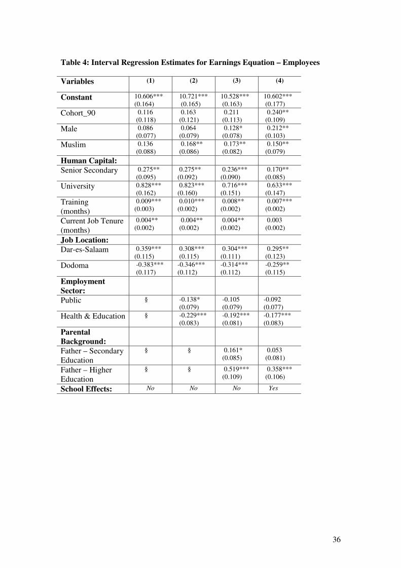
The interval regression model estimates for the employees’ sample are reported in

table 4. A brief review of the diagnostics is in order as a prelude to a more detailed

discussion of the earnings equation estimates themselves. All the estimated models

comfortably pass the RESET. The result for normality is more mixed and on the

borderline for our preferred specification (4) in table 4. We believe, however, it is

innocuous to infer that the assumption of normality provides a reasonable

approximation for the unobservables governing the determination of the earnings

process for employees. The null hypothesis of homoscedasticity is decisively rejected

for the four estimated models and the Huber (1967) adjustment is thus used to

construct a robust variance-covariance matrix for the coefficient estimates. The

goodness of fit measure for our preferred specification is healthy by the standards of

cross-sectional earnings equations. However, it should be stressed it does not have

the conventional interpretation associated with the R2 generated using the more

conventional OLS procedure.26

[Table 4]

The estimated coefficient for the selection correction term is poorly determined in all

four specifications and suggests that the sample of employees comprise a random

drawing from the sample of school-leavers available to us. In addition, it is worth

noting that the estimated selection effect is not materially affected by the inclusion of

additional regressors in the earnings equation. This tentatively suggests that the result

in regard to selection bias may be insensitive to the set of identifying instruments

used.

The discussion of the estimates will primarily focus on our preferred specification (4)

in table 4 but cross-reference will be made to other specifications where necessary.

The cohort effect achieves statistical significance within the 5% level for our 26 In other words, we cannot use these measures to infer that a certain proportion of the variation in monthly earnings is explained by variation in the explanatory variables. The measure provides the proportional change in the likelihood function consequent in the inclusion of the explanatory variables.

20

preferred specification. This variable is designed to proxy for age effects and suggest

that the average ceteris paribus earnings for the 1990 cohort are 27% higher than for

the more recent 1995 cohort of leavers. There is also some evidence of gender and

religious advantage in employee monthly earnings with the male premium estimated

at 23.6% and Muslims securing about 16% more than non-Muslims, on average and

ceteris paribus. The gender effect is perhaps not surprising although it is also

interesting to note that wage employment opportunities grew faster for female

completers over the 1990s than their male counterparts. The wage premium associated

with the Muslim respondents in the survey may in part reflect the influence of social

networks related to the school (but not directly captured by the school effects) that

provide good jobs for completers.

There is a sizeable return of nearly 34% for those with jobs located in Dar-es-Salaam

compared to the relatively heterogeneous base comprising all other Tanzanian areas

other than Dodoma. This in part may reflect cost of living differences given the much

higher cost of living in Dar es Salaam compared to other (including urban) areas in

Tanzania. Approximately one-third of the employees in the sample work in the health

and education sector and earn, on average and ceteris paribus, 16.2% less in monthly

terms than workers in other sectors.27 Given the recent expansion in educational

access in Tanzania more secondary school completers will be absorbed into the

education sector as teachers, but the lower wages are unlikely to attract the best

candidates in this sector. The monthly earnings of public sector workers, however, are

not statistically different from their private sector counterparts.

We now turn to the estimates for the human capital measures. The estimated

coefficient for the training variable is robust across all the reported specifications and

the estimates are generally invariant to the inclusion of the additional controls for

parental background and school effects. In interpreting the estimate it is useful to

translate the effect into an annualised return. Thus, an additional year of general

training raises monthly earnings by 8.4%, on average and ceteris paribus. The

estimated effect for on-the-job experience raises monthly earnings by a more modest 27 The inclusion of these controls might also proxy for the number of hours worked per month as these are likely to be lower in the public, health and education sectors. However, the crudeness of this proxy measure is readily acknowledged.

21

4.8% per annum in the first three specifications reported but becomes borderline in

terms of statistical significance when the school controls are introduced in the final

preferred specification.28 Given such further training and education generally involves

a substantial investment of the part of these individuals and their parents, it is salutary

to note that such investments appear, on the average, to have some pay-off in the

formal sector.

The estimated returns for the educational qualifications are mildly sensitive to the

gradual inclusion of additional controls across the different specifications. The

introduction of parental and school controls attenuates the estimated effect for the

senior secondary qualification but it retains statistical significance at a conventional

level in our preferred model. A similar pattern is evident for the estimated effect for

university graduates but the attenuation is most pronounced with the introduction of

the father’s educational background variables. The estimated coefficient for a

university graduate falls by 0.11 log points or over one-tenth in value with the

inclusion of the two measures for father’s education. This does highlight the

importance of controlling for parental background when attempting to obtain

informative estimates for the returns to educational qualifications. A more detailed

discussion on the returns to the educational qualifications is provided below.

An examination of the estimated effect of a father’s educational background on

earnings, however, is perhaps important in its own right. The estimates in our

preferred specification suggests that individuals whose fathers have higher education

earn 43% more than those individuals whose fathers have less than secondary

education, on average and ceteris paribus. There are a number of ways of interpreting

this result. It may reflect the fact that educated parents are more effective at

inculcating in their children the skills that are ultimately well rewarded in the

Tanzanian labour market. Alternatively, it may be the case that individuals from

those families whose fathers are highly educated can exploit informal networks in

securing the better-paid jobs. Both interpretations could be viewed as providing

28 Controls designed to capture previous labour force experience in months in wage employment, self-employment or unemployment yielded poorly determined effects in the reported specifications and were consequently dropped.

22

mechanisms that encourage an inter-generational transfer of inequality. It is also

worth noting that the inclusion of the school controls reduces the father’s higher

educational effect by almost one-third. This may suggest that the school system, as

captured by our school controls, plays some role in ossifying such inter-generational

inequality.

5.2 Earnings Equation – The Self-employed

The interval regression model estimates for the sample of self-employed are reported

in table 5. In contrast to the regression models for the employees, the performance in

regard to the diagnostics is considerably poorer. In terms of our preferred

specification, the model again passes the RESET but registers a more decisive

rejection of normality. There is also a failure in regard to heteroscedasticity. In

addition, the fits of the regression models are poor by any standard and few of the

estimated coefficients are well determined. There are a couple of exceptions to this

general statement and one is reserved for the estimated selection effect. The negative

coefficient is consistent with the presence of positive selection given the construction

and derivation of the selection term in this application (see Lee (1983)). The point

estimate for the selection effect suggests that those who select into self-employment

earn about 18% more in bi-annual earnings than those drawn at random from the

population of school-leavers.29

[Table 5]

An interesting feature of the regression estimates for the self-employed draws on a

comparison with table 4. In particular, the estimate for the standard error of the

regression is considerably higher for the self-employed than for employees. Part of

this may be attributable to the use of more earnings intervals in the self-employed

application but this cannot explain all of the difference.30 This could be taken to

29 This is computed as the product of the negative value of the selection coefficient (0.375) multiplied by the average value of the selection term (0.483). This yields the average selection effect which equals 0.181 in this case. 30 Using the preferred specification (4) in both tables the F-test for the difference in variances is computed at 2.54 ~ F(191,378). The null hypothesis of a common variance in residual earnings is thus decisively rejected in this case.

23

confirm to some extent that unobservable prices and quantities are considerably more

important in earnings determination for self-employed than for employees.

Ignoring school effects and the selection effect already discussed, only three of the

estimated coefficients for the self-employed achieve statistical significance at a

conventional level: current job tenure, wage employment experience and holding a

university qualification. The amount of experience acquired in wage employment

enhances the bi-annual earnings of the self-employed with an additional year raising

self-employed income by 24%, on average and ceteris paribus. The comparable

effect for current job tenure is 8.4%. On the face of it, the possession of a university

degree yields sizeable benefits for the self-employed. However, it is worth noting that

only a small number of the self-employed hold such a qualification (8 out of 214) and

these estimates may reflect more the characteristics of this small group than informing

generally about returns to this measure of human capital in the self-employed sector.

It is important to complete this sub-section by noting those factors that appear to play

no role in earnings determination for the self-employed. These include gender and

religious affiliation and this could be tentatively taken to suggest little evidence of

consumer-based discrimination in our Tanzanian sample. Earnings are reasonably flat

in terms of the training measure used and the age of the individual as measured by the

school-leaver cohort control. There appears no role for parental education in earnings

determination in the self-employed sector. There is no evidence of regional variation

in self-employed earnings with no indication that thick market externalities are

exploitable in the country’s capital city for the sample of self-employed. In addition,

it also appears to matter little whether the individual works on ‘own-account’ or

employs others.31

The school effects and the returns to qualifications for the self-employed will be

discussed in greater detail in the next two sub-sections.

31 There are reasons for believing that our measure of this may not be accurately capturing this type of distinction.

24

5.3 The Estimated School Effects

One motivation for the inclusion of the school fixed effects is to control, inter alia, for

schooling quality in terms of its potential effect on education returns and on earnings

more generally. Their inclusion is also motivated by a sense that they might also

capture labour market network effects. The inclusion of the school controls tends to

reduce both the return to senior secondary schooling and to a university qualification

but induces a sharper reduction in the former relative to the latter.32 This is a relatively

intuitive result and highlights the importance of controlling for schooling quality in

computing rates of return to schooling qualifications. It is apparent that parental

educational background is more important to the estimated university returns than

secondary schooling quality.

The school effects can be interrogated more thoroughly by normalizing the ten

estimated school effects as a deviation from an overall school weighted average

effect. This transformation has intuitive appeal in that the estimated earnings

differences are now relative to an overall average rather than an arbitrary base group

and are thus more easily interpretable. This approach follows the approach adopted

by Krueger and Summers (1988) in the literature on inter-industry wage differentials.

If we define the school effect from the interval regression model for the kth school as

γk the deviation is expressed as:

γk – �=

10

1j

πjγj [8]

where πj is the proportion of the sample in the jth school. The corresponding sampling

variances are computed as per Zanchi (1998).33 Table 6 reports the estimated

deviations for the ten schools for both wage employees and the self-employed.

[Table 6]

32 In Table 4 the estimated coefficient for the senior secondary qualification reduced by one-quarter with the inclusion of school fixed effects, while the comparable estimate for the university qualification reduces by just under one-tenth. 33 See also Haisken-DeNew and Schmidt (1997) for a more detailed discussion.

25

The ceteris paribus earnings for those in eight of the ten schools are not statistically

different from the average for either the employee or the self-employed groups.

However, there are two schools for which the earnings of their alumni (both

employees and the self-employed) are different from the overall average. One school

is well above and the other well below the average. In terms of the employee group

the graduates of one school earn ceteris paribus about 59% more than the average,

while graduates from the less favoured school earn ceteris paribus about 38% less

than the average. The contrast in earnings performance between the graduates from

the two schools appears starker in terms of the point estimates for the self-employed

but there is no statistical difference in these effects across the two employment sectors

– either individually or jointly. In addition, the estimated Spearman rank order

correlation coefficient for school rankings across the two sectors on the basis of the

earnings of their alumni is 0.71 and this is statistically significant from zero at the 5%

level.

It is evident that the school an individual attends matters in a number of cases but why

it matters may be too complex to unravel satisfactorily given the data to hand. The

more favourable school identified in table 6 is a private co-educational non-boarding

school based in an urban area of Tanzania. The less favourable school is a public

school but identical to the other school in respect of the characteristics noted. In

addition, the national ranking of the public school in the 1990s actually appears

superior in comparison to that of the private school. However, those that attended the

latter tended to be disproportionately drawn from backgrounds where the father had

either secondary or higher education. Thus, it could legitimately be argued that this

particular school effect is partly capturing a socio-economic background factor that is

not entirely attributable to an independent school quality effect. It might capture

labour market network effects in the sense that graduates from this particular school

are better able to exploit a network of former graduates who have perhaps attained

influential positions in the Tanzanian labour market. It is worth noting that school

eight in table 6 is also a private school, albeit in a rural area, but its alumni were

drawn from backgrounds where the father was less likely to have education beyond a

primary level.

26

5.4 Estimated Private Rates of Return to Educational Qualifications

We now turn to an examination of the estimated private rates of return for the two

educational qualifications used here – senior secondary and university. These are

computed using the differences in the estimated coefficients between adjacent

qualifications divided by the difference in years. If we define the interval regression

earnings model parameter for a university qualification as γU and for senior secondary

as γS, the rate of return (RoR) to a university qualification is computed as:

RoR – University Qualification = YearsYears

SU

S-U- γγ

[9]

where UYears is total years in education to acquire a university qualification and SYears

is the corresponding number of years taken to acquire a senior secondary

qualification. The rate of return to senior secondary schooling can then be computed

as:

RoR – Senior Secondary Qualification = Years Years

S

J-S γ

[10]

where JYears is total years in education to acquire a junior certification qualification.

The sampling variances for the estimated rates of return are easily computed using the

conventional formula.

The estimated rates return reported in table 7 are the exponentiated versions of [9] and

[10] expressed in percentages and the corresponding sampling variances are

constructed using the delta method. In respect of employees the point estimate for the

senior secondary qualification is just under nine per cent but is situated within a large

confidence interval and is only significant at the 10 per cent level. The comparable

point estimate for the self-employed is close to five per cent but is even more

imprecisely estimated. At a conventional level of statistical significance, the

proposition that the sample data were generated from an underlying population with a

zero return for the senior secondary qualification cannot be rejected for the self-

employed.

27

[Table 7]

The rate of return for a university qualification for the employees is well determined.

The point estimate suggests an annualised rate of return of 16.7%. The comparable

point estimate for the self-employed is larger but again more imprecisely estimated.34

As noted earlier the computed rate of return for the self-employed also warrants

caution given the small cell size used to compute it.35

As noted in the introduction to this paper, the evidence on the estimated rates of return

to education in Tanzania is relatively sparse. Nevertheless, it would be useful to

situate our findings on returns within the broader context of the literature. In common

with the more general literature on returns to education researchers have computed

both marginal returns to an additional year in education and returns to qualifications

for Tanzania. In terms of the former Psacharopoulos (1994) reported an estimate of

12%, while in more recent work Söderbom, Teal, Wanbugu and Kahyarara (2003),

using data for the Tanzanian manufacturing sector, provided estimates in a range from

12% for young workers to 17% for older workers. This study also reported some

evidence of an increase in the estimated educational returns in Tanzania over the last

decade.

The literature on estimates for returns to qualifications, as reported in table 2, is even

less extensive for Tanzania. The point estimates obtained are dimensionally

comparable to the findings of Mason and Khandker (1997) which used the Tanzanian

Labour Force Survey (LFS) from 1991. The estimates reported by a number of

authors for the returns to secondary schooling are broadly in comport with our

findings in this study. However, the point estimate for the university qualification

34 The estimated rate of return to a university qualification obtained using the 1991 LFS is computed at almost 16% but is also based on a very small cell size. The point estimate for the rate of return to secondary schooling is estimated to be indistinguishable from zero using the same source. Both these estimates tie in with our findings from the tracer study. 35 In order to examine whether there was any evidence of variation in estimated returns across gender groups, we introduced two gender interactions in the educational qualifications to specification (4) for both employment types. The two interactions were found to be statistically insignificant in both equations with the chi-squared statistics computed at 0.04 and 0.36 for the employees and the self-employed respectively.

28

obtained using the tracer study data is higher than that obtained using the LFS data

but the LFS-based point estimates comfortably lie within even the most modest

confidence interval generated using our sample of employees.

29

6. Conclusions

A key finding of our analysis is that the point estimates for the private returns to a

university education are higher compared to senior secondary and this finding is

compatible with the notion of a convex relationship between earnings and educational

level as recently posited for Tanzania by Söderbom et al. (2003). On the basis of a

crude comparison with previous studies, there is no indication that the estimated rates

of return to senior secondary and university qualifications have actually increased

over the last decade. Indeed, there is evidence of some degree of stability in these

returns over time. However, we do accept that such a comparison can only provide a

tentative rather than definitive insight into the temporal movement in the returns to a

university education.

Further education and training undertaken by secondary school leavers, once formal

education is completed, appears to increase wage employment earnings significantly.

This is a comforting result given the heavy investments secondary school-leavers

make in further education and training. The respondents in our survey, who had

completed junior secondary education in 1990 (1995), had spent approximately 3 (2)

years between 1990 (1995) and 2001 in further education and training (see Al-

Samarrai and Bennell (2003)). Unfortunately it was not possible to dis-aggregate the

months of training between their different types. A deeper understanding of which

types of training have the biggest impact on earnings would be an interesting avenue

for future research but is not pursued here.

Information contained in the tracer surveys allowed us to include controls for father’s

educational background and a set of school controls designed to proxy for school

quality and potential labour market network effects. The inclusion of school fixed

effects reduced the estimated rates of return to education. The analysis shows that the

school an individual attends is important and this in part may be due to labour

network effects with leavers for particular schools having preferential access to better

paying jobs through school or other contacts. A further key finding in our analysis

30

relates to the role of father’s education in determining the estimated returns to a

particular qualification. If we exclude these controls from the employee earnings

equation and re-compute the rates of return for the two qualifications, the rate of

return to senior secondary is unaffected while the estimated return to a university

qualification rises by 1.5 percentage points.36 This serves to emphasize the potential

confounding role of parental background in such estimates. We would argue that a

failure to control for such background variables potentially leads to an over-statement

in the estimated returns to at least university qualifications.

In general, we found little evidence of well determined human capital effects in the

earnings determination process in the self-employment sector. It is acknowledged

that university education appeared to exert a statistically significant impact on self-

employment earnings but the small cell size for this group merits interpretational

caution. The estimated self-employment earnings equation was found to be poorly

determined. These facts are hardly surprising given the traditional type of self-

employment activities in which secondary school leavers were engaged. Typically,

secondary school leavers were working as small-scale vendors (i.e., buying and

selling goods) with relatively few additional staff (see Al-Samarrai and Bennell

(2003)). It is unlikely that post-primary education will be of much benefit in these

activities. Furthermore, secondary school leavers in Tanzania approached self-

employment as a queuing strategy for waged employment opportunities. Given the

increasing numbers of secondary school-leavers entering self-employment these

findings are worrying from a policy perspective. Secondary school-leavers

interviewed for the survey indicated that they were at least partially aware of the lack

of relevance of their secondary education for self-employment as only a minority

agreed that the secondary school curriculum was relevant (see Al-Samarrai and

Bennell (2003)).

Finally, the estimates we obtained for the private rates of return to both secondary and

university qualifications for wage employees were comparable in magnitude to those

obtained using the Tanzanian Labour Force Survey. Our empirical evidence suggests

36 This is based on excluding the parental controls from specification (4) and re-computing the rate of return as per expression [10].

31

that the rates of return to educational qualifications are not small and at the margin

provide an investment incentive. However, despite an extremely small secondary and

university education system the private rates of return to education in the Tanzanian

wage employment sector are low compared to other countries in the region.

32

References Al-Samarrai, S. and Bennell, P. (2003), Where has all the education gone in Africa?. Brighton: Institute of Development Studies and Knowledge and Skills for Development Bennell, P. (1996), Rates of Return to Education: Does the conventional Pattern Prevail in Sub-Saharan Africa, World Development, Vol. 24(1), pp. 183-199. Bennell, P. (1994), Jobs for the boys? The employment experiences of secondary school leavers in Zimbabwe, Journal of Southern African Studies, Vol. 20 (2) pp. 301–15 Bennell, P. and Ncube, M. (1993), Education and training outcomes: University graduates in Zimbabwe during the 1980s, Zimbabwe Journal of Educational Research, Vol. 5(2), pp. 107–123. Card, D. (1999), The Causal Effect of Education on Earnings, Chapter 30 in Handbook of Labor Economics, Vol.3, edited by O.Ashenfelter and D.Card. Chesher, A. and Irish M. (1987) Residual Analysis in the Grouped and Censored Normal Regression Model, Journal of Econometrics, Vol. 34, pp. 33–61. Haisken-DeNew, J. P. and C. M. Schmidt (1997), Inter-Industry and Inter-Region Differentials: Mechanics and Interpretation, Review of Economics and Statistics Vol. 79, pp. 516-521. Heckman, J. (1979), Sample Selection Bias as a Specification Error, Econometrica Vol. 47, pp. 153-161. Huber, P.J. (1967) The Behaviour of Maximum Likelihood Estimates Under Non-standard Conditions in Proceedings of the Fifth Berkeley Symposium on Mathematical Statistics and Probability. Berkeley, CA: University of California Press, 1, pp. 221 – 223. Glewwe, P. (2002), Schools and Skills in Developing Countries: Education Policies and Socioeconomic Outcomes, Journal of Economic Literature Vol. 150, No 2, pp. 436-482. Greene, W. (2000) Econometric Analysis (4th edition) New York, Macmillan. Kaijage, E.S. (2000), Faculty of Commerce and Management graduates and their employers: A tracer study, Dar es Salaam: University of Dar es Salaam Knight, J.B. and Sabot, R.H. (1990), Education, Productivity and Inequality. New York: Oxford University Press.

33

Knight, J.B. and Sabot, R.H. (1981), The Returns to Education: Increasing with Experience of Decreasing with Expansion?. Oxford Bulletin of Economic Statistics Vol. 43, pp. 51-71. Krueger, A. B. and L. H. Summers (1988), Efficiency Wages and the Inter-Industry Wage Structure, Econometrica Vol. 56(2), pp. 259-293. Lee L. (1983), Generalized models with selectivity, Econometrica Vol. 51, pp. 507 – 512. LIMDEP 7.0 (1998) Econometric Software, Inc. Mason, A.D. and Khandker, S.R. (1997), Household Schooling Decisions in Tanzania, Washington DC: World Bank; Poverty, Gender and Public Sector Management Department. Mayanja, M.K. and Nakayiwa, F. (1997), Employment Opportunities for Makerere University Graduates: Tracer Study, Kampala: Makerere University, School of Post Graduates and Research MOEC (various years), Basic Education Statistics in Tanzania (BEST). Dar es Salaam: Ministry of Education and Culture.

Mukyanuzi, F. (2003). Where has all the education gone in Tanzania? Brighton, IDS and Knowledge and Skills for Development.

Narman, A., 1992, Trainees at Moshi National Vocational Training Centre: Internal achievements and labour market adoption: Final report on a tracer study project in Tanzania, Stockholm: Swedish International Development Agency Orme, C. (1990). The small sample performance of the information matrix test, Journal of Econometrics, Vol. 46, pp.309-331. Peters, S. (2000) On the use of the RESET test in microeconometric models, Applied Economics Letters, Vol. 7, pp. 361–365. Planning Commission (2000), Labour Force Survey, draft report, Dar es Salaam: Government Printers Planning Commission (1993), Labour Force Survey, report, Dar es Salaam: Government Printers. Psacharopoulos, G. and Patrinos, H. (2004), Returns to Investment in Education: A Further Update’, Washington D.C: World Bank Policy Research Working Paper No. 2881, The World Bank. Psacharopoulos, G. and Loxley, W. (1985), Diversified Secondary Education and Development: Evidence from Colombia and Tanzania. Baltimore: John Hopkins Press.

34

Ramsey, J.B. (1969) Tests for specification errors in classical linear least-squares regression analysis, Journal of the Royal statistical Society: Series B, Vol. 31, pp. 350 – 71 Samoff, J. (1987), School Expansion in Tanzania: Private Initiatives and Public Policy, Comparative Education Review Vol. 31, pp. 333-360. Söderbom, M., Teal, F., Wambugu, A. and G. Kahyara (2003), The Dynamics of Returns to Education in Kenyan and Tanzanian Manufacturing, CSAE working paper WPS/2003-17, Oxford University Stewart, M. (1983), On least squares estimation when the dependent variable is grouped, Review of Economic Studies, Vol.50, pp.737-753. UNESCO (2003). Global Monitoring Report: Gender and Education for All, the Leap to Equality, Paris. UNESCO

Zanchi, L. (1998), Interindustry wage Differentials in Dummy Variable Models, Economics Letters, Vol. 60, pp. 297-301.

35

Table 1: Highest level of education achieved in Tanzanian population aged 25+ Education level Male Female Total No education 15.1 35.7 25.7 Incomplete primary 23.1 18.2 20.6 Primary 46.9 38.6 42.6 Junior secondary 8.8 4.1 6.4 Senior secondary 3.4 0.8 2.0 University degree 0.0 0.0 0.0 Other 2.8 2.6 2.7 Total 100.0 100.0 100.0

Notes to Table 1: Source: Authors’ calculations from Human Resource Development Survey 1993. Notes: The proportions given in the table are weighted proportions from the survey that inflate the individual level data to nationally representative figures. Table 2: Private Rates of Return – Summary of Estimates (%) Author(s) Year and source of Data Primary Secondary University Mason & Khandker (1997) 1991 – Labour Force Survey 7.9 8.8 § Authors’ own calculations 1991 – Labour Force Survey 1.4 8.7/9.8 10.8 Knight and Sabot (1981 and 1990) 1971 and 1980 - Survey of

manufacturing sector employees

2.1 7.9 §

Psacharopoulos and Loxley (1985) 1982 – Tracer survey of 1981 secondary school leavers

§ 3.1 §

Notes to table 2: (a) § denotes not applicable or not reported. (b) all rates of return are for wage employment in the formal sector (c) Differences in the rates of return reported from the 1991 Labour Force Survey are due to

different methodologies. The Mason and Khandker returns are calculated using the full method.

(d) The authors’ own calculations are rates of return based on Mincerian regression models. The secondary education is disaggregated by junior and senior secondary, hence the two estimates reported.

(e) For comparability purposes the results reported in this table do not include adjustments to the returns for ability etc.

(f) The primary rate of return for Knight and Sabot is from Knight and Sabot (1981) and for secondary from Knight and Sabot (1990)

Table 3: Tracer Survey Response Rates Male Female Total

Total Traced 510 455 965 Interviewed 466 408 874 Postal 7 9 16 Parents 25 25 50 Abroad 2 2 4 Deceased 10 11 21

Not traced 16 19 35 Total sample 526 474 1000 Response rate (%) 97 96 97

36

Table 4: Interval Regression Estimates for Earnings Equation – Employees Variables (1)

(2) (3) (4)

Constant 10.606*** (0.164)

10.721*** (0.165)

10.528*** (0.163)

10.602*** (0.177)

Cohort_90 0.116 (0.118)

0.163 (0.121)

0.211 (0.113)

0.240** (0.109)

Male 0.086 (0.077)

0.064 (0.079)

0.128* (0.078)

0.212** (0.103)

Muslim 0.136 (0.088)

0.168** (0.086)

0.173** (0.082)

0.150** (0.079)

Human Capital:

Senior Secondary 0.275** (0.095)

0.275** (0.092)

0.236*** (0.090)

0.170** (0.085)

University 0.828*** (0.162)

0.823*** (0.160)

0.716*** (0.151)

0.633*** (0.147)

Training (months)

0.009*** (0.003)

0.010*** (0.002)

0.008** (0.002)

0.007*** (0.002)

Current Job Tenure (months)

0.004** (0.002)

0.004** (0.002)

0.004** (0.002)

0.003 (0.002)

Job Location:

Dar-es-Salaam 0.359*** (0.115)

0.308*** (0.115)

0.304*** (0.111)

0.295** (0.123)

Dodoma -0.383*** (0.117)

-0.346*** (0.112)

-0.314*** (0.112)

-0.259** (0.115)

Employment Sector:

Public § -0.138* (0.079)

-0.105 (0.079)

-0.092 (0.077)

Health & Education § -0.229*** (0.083)

-0.192*** (0.081)

-0.177*** (0.083)

Parental Background:

Father – Secondary Education

§ § 0.161* (0.085)

0.053 (0.081)

Father – Higher Education

§ § 0.519*** (0.109)

0.358*** (0.106)

School Effects: No No No Yes

37

Table 4 (Cont’d) Selection Correction Term

-0.057 (0.118)

-0.082 (0.114)

-0.093 (0.108)

-0.150 (0.113)

∧σ

0.699 0.684 0.659 0.626

Pseudo-R2 0.106 0.114 0.132 0.156

RESET ~ χ23 0.214

(0.975) 2.267 (0.519)

1.154 (0.764)

1.496 (0.683)

Homoscedasticity ~ χ2

k 40.706*** (0.000)

46.869*** (0.000)

37.551*** (0.000)

61.601*** (0.000)

Normality~ χ22 2.348

(0.309) 6.361** (0.042)

3.417 (0.181)

4.774* (0.092)

Observations 402 402 402 402 Notes to table 4: (a) The earnings measure relates to current monthly income. (b) The lower and upper bounds used in estimation expressed in Tanzanian shillings (000s) are [-∞, 50],[50 ,100],[100,150],[150,200], [200,250], [250,300],[300,400], [400,+∞]. The natural logarithms of the finite interval boundaries were used in specifying the model’s likelihood function. (c) The reported estimates are based on the maximum likelihood procedure. The estimated standard errors reported in parentheses are based on the Huber (1967) adjustment. (d) ***,** and * denote statistical significance at the 1%, 5% and 10% level respectively using two-tailed tests. (e) § denotes not applicable in estimation for given model. (f) For the heteroscedasticity test the degrees of freedom are k and are determined by the number of variables in each specification. (g) The values in parentheses beneath the diagnostic test values are the significance levels of the tests.

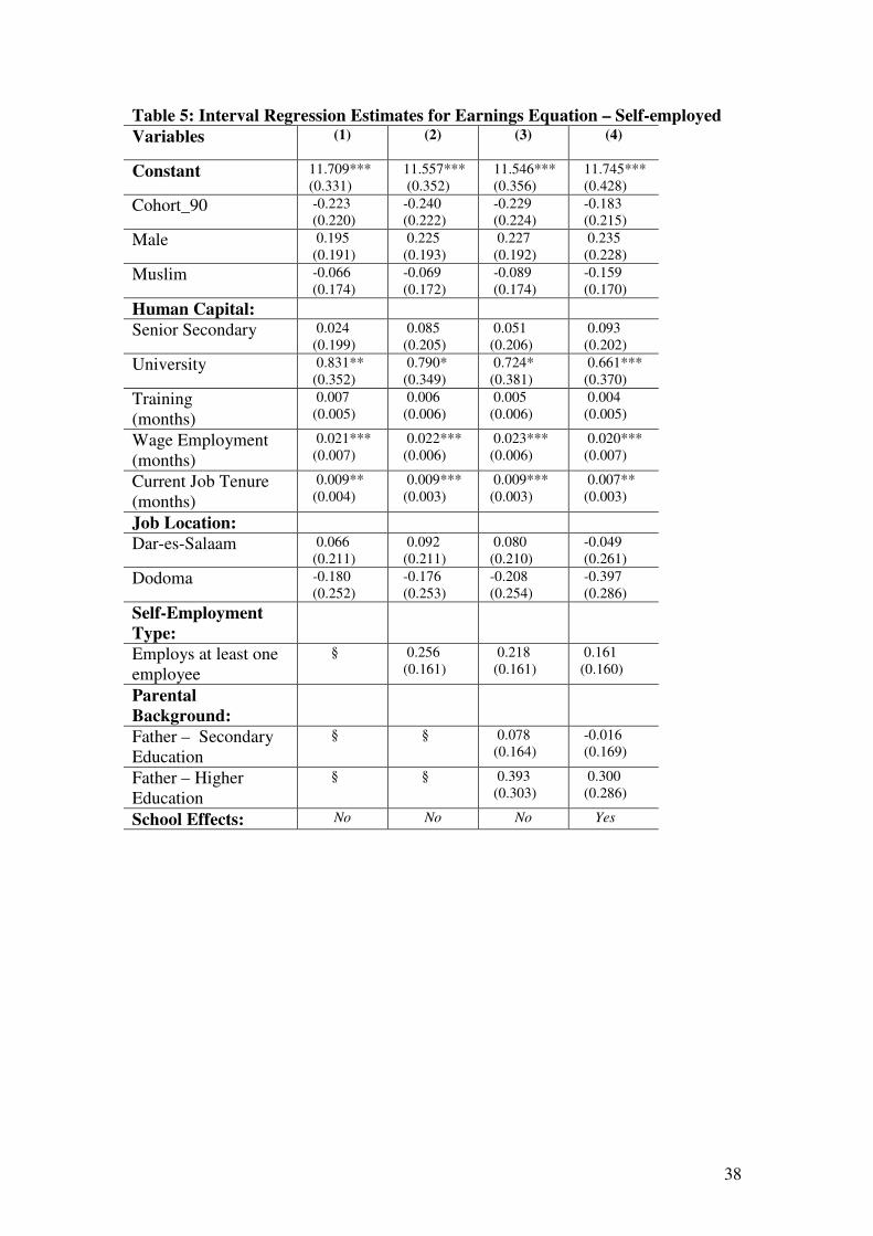
38

Table 5: Interval Regression Estimates for Earnings Equation – Self-employed Variables (1)

(2) (3) (4)

Constant 11.709*** (0.331)

11.557*** (0.352)

11.546*** (0.356)

11.745*** (0.428)

Cohort_90 -0.223 (0.220)

-0.240 (0.222)

-0.229 (0.224)

-0.183 (0.215)

Male 0.195 (0.191)

0.225 (0.193)

0.227 (0.192)

0.235 (0.228)

Muslim -0.066 (0.174)

-0.069 (0.172)

-0.089 (0.174)

-0.159 (0.170)

Human Capital:

Senior Secondary 0.024 (0.199)

0.085 (0.205)

0.051 (0.206)

0.093 (0.202)

University 0.831** (0.352)

0.790* (0.349)

0.724* (0.381)

0.661*** (0.370)

Training (months)

0.007 (0.005)

0.006 (0.006)

0.005 (0.006)

0.004 (0.005)

Wage Employment (months)

0.021*** (0.007)

0.022*** (0.006)

0.023*** (0.006)

0.020*** (0.007)

Current Job Tenure (months)

0.009** (0.004)

0.009*** (0.003)

0.009*** (0.003)

0.007** (0.003)

Job Location:

Dar-es-Salaam 0.066 (0.211)

0.092 (0.211)

0.080 (0.210)

-0.049 (0.261)

Dodoma -0.180 (0.252)

-0.176 (0.253)

-0.208 (0.254)

-0.397 (0.286)

Self-Employment Type:

Employs at least one employee

§ 0.256 (0.161)

0.218 (0.161)

0.161 (0.160)

Parental Background:

Father – Secondary Education

§ § 0.078 (0.164)

-0.016 (0.169)

Father – Higher Education

§ § 0.393 (0.303)

0.300 (0.286)

School Effects: No No No Yes

39

Table 5 (cont’d) Selection Correction Term

-0.448** (0.199)

-0.455** (0.203)

-0.467** (0.209)

-0.483** (0.200)

∧σ

1.055 1.047 1.042 0.997

Pseudo-R2 0.032 0.032 0.034 0.052

RESET ~ χ23 15.878***

(0.001) 8.535** (0.036)

6.479* (0.090)

4.132 (0.248)

Homoscedasticity ~ χ2

k 20.803** (0.035)

21.956** (0.038)

23.137* (0.058)

41.529** (0.010)

Normality~ χ22 4.780*

(0.092) 6.448** (0.040)

5.511* (0.063)

13.479*** (0.001)

Observations 214 214 214 214 Notes to table 5: (a) The earnings measure relates to self-employed earnings received in the last six months. (b) The lower and upper bounds used in estimation expressed in Tanzanian shillings (000s) are [-∞, 100],[100,150],[150,200],[200,250], [250,300], [300,350],[350,400],[400,500],[500,800],[800,+∞]. The natural logarithms of the finite interval boundaries were used in specifying the model’s likelihood function. (c) The reported estimates are based on the maximum likelihood procedure. The estimated standard errors reported in parentheses are based on the Huber (1967) adjustment. (d) ***,** and * denote statistical significance at the 1%, 5% and 10% level respectively using two-tailed tests. (e) § denotes not applicable in estimation for given model. (f) For the heteroscedasticity test the degrees of freedom are k and are determined by the number of variables in each specification. (g) The values in parentheses beneath the diagnostic test values are the significance levels of the tests.

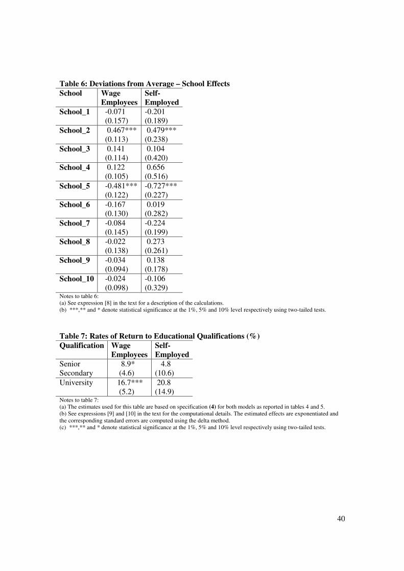
40

Table 6: Deviations from Average – School Effects School

Wage Employees

Self-Employed

School_1 -0.071 (0.157)

-0.201 (0.189)

School_2 0.467*** (0.113)

0.479*** (0.238)

School_3 0.141 (0.114)

0.104 (0.420)

School_4 0.122 (0.105)

0.656 (0.516)

School_5 -0.481*** (0.122)

-0.727*** (0.227)

School_6 -0.167 (0.130)

0.019 (0.282)

School_7 -0.084 (0.145)

-0.224 (0.199)

School_8 -0.022 (0.138)

0.273 (0.261)

School_9 -0.034 (0.094)

0.138 (0.178)

School_10 -0.024 (0.098)

-0.106 (0.329)

Notes to table 6: (a) See expression [8] in the text for a description of the calculations. (b) ***,** and * denote statistical significance at the 1%, 5% and 10% level respectively using two-tailed tests. Table 7: Rates of Return to Educational Qualifications (%) Qualification

Wage Employees

Self-Employed

Senior Secondary

8.9* (4.6)

4.8 (10.6)

University 16.7*** (5.2)

20.8 (14.9)

Notes to table 7: (a) The estimates used for this table are based on specification (4) for both models as reported in tables 4 and 5. (b) See expressions [9] and [10] in the text for the computational details. The estimated effects are exponentiated and the corresponding standard errors are computed using the delta method. (c) ***,** and * denote statistical significance at the 1%, 5% and 10% level respectively using two-tailed tests.

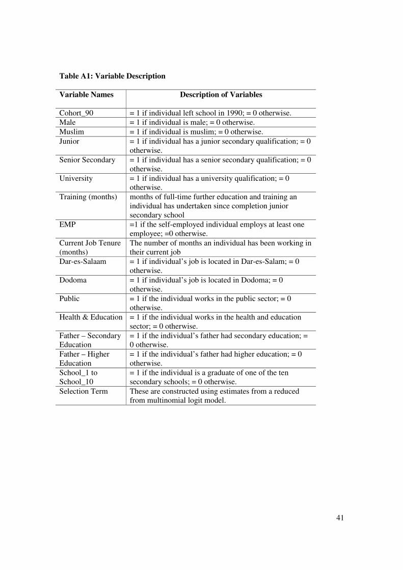
41

Table A1: Variable Description Variable Names Description of Variables

Cohort_90 = 1 if individual left school in 1990; = 0 otherwise. Male = 1 if individual is male; = 0 otherwise. Muslim = 1 if individual is muslim; = 0 otherwise. Junior = 1 if individual has a junior secondary qualification; = 0

otherwise. Senior Secondary = 1 if individual has a senior secondary qualification; = 0

otherwise. University = 1 if individual has a university qualification; = 0

otherwise. Training (months) months of full-time further education and training an

individual has undertaken since completion junior secondary school

EMP =1 if the self-employed individual employs at least one employee; =0 otherwise.

Current Job Tenure (months)

The number of months an individual has been working in their current job

Dar-es-Salaam = 1 if individual’s job is located in Dar-es-Salam; = 0 otherwise.

Dodoma = 1 if individual’s job is located in Dodoma; = 0 otherwise.

Public = 1 if the individual works in the public sector; = 0 otherwise.

Health & Education = 1 if the individual works in the health and education sector; = 0 otherwise.

Father – Secondary Education

= 1 if the individual’s father had secondary education; = 0 otherwise.

Father – Higher Education

= 1 if the individual’s father had higher education; = 0 otherwise.

School_1 to School_10

= 1 if the individual is a graduate of one of the ten secondary schools; = 0 otherwise.

Selection Term These are constructed using estimates from a reduced from multinomial logit model.

42

Table A2: Summary Statistics Wage employed Self employed

Variable Mean Std. Dev. Min Max Mean

Std. Dev. Min Max

earnings 11.39 0.87 10.13 13.30 12.23 1.01 10.82 13.71

Cohort_90 0.65 0 1 0.53 0 1

Male 0.48 0 1 0.69 0 1

Muslim 0.25 0 1 0.30 0 1

Senior Secondary 0.29 0 1 0.25 0 1

University 0.13 0 1 0.04 0 1

Training (months) 20.48 18.95 0 96 10.01 0 74 Current Job Tenure (months) 44.55 28.85 2 126 54.11 3 132

EMP 0.58 0 1

Dar-es-Salaam 0.59 0 1 0.57 0 1

Dodoma 0.24 0 1 0.26 0 1

Public 0.36 0 1 0.00 0 0

Health & Education 0.31 0 1 0.03 0 1

Father – Secondary Education 0.31 0 1 0.30 0 1

Father – Higher Education 0.19 0 1 0.09 0 1

School_1 0.08 0 1 0.17 0 1

School_2 0.09 0 1 0.12 0 1

School_3 0.12 0 1 0.07 0 1

School_4 0.12 0 1 0.03 0 1

School_5 0.08 0 1 0.07 0 1

School_6 0.09 0 1 0.09 0 1

School_7 0.07 0 1 0.15 0 1

School_8 0.12 0 1 0.10 0 1

School_9 0.09 0 1 0.13 0 1

Selection term

sample size 402 214 Notes to table A2: (a) log earnings are the mean of the mid-point of the intervals described in the methodology section and are not actually used in the analysis.