Editorial Board - UPT · Editorial Board • Prof. Dr. Eng ... • Prof. Dr. Eng. Andre QUINQUIS,...
47
Editorial Board • Prof. Dr. Eng. Ioan NAFORNITA, Editor-in-chief • Prof. Dr. Eng. Virgil TIPONUT • Prof. Dr. Eng. Alexandru ISAR • Prof. Dr. Eng. Dorina ISAR • Prof. Dr. Eng. Traian JURCA • Prof. Dr. Eng. Aldo DE SABATA • Prof. Dr. Eng. Florin ALEXA • Prof. Dr. Eng. Radu VASIU • Assist. Dr. Eng. Maria KOVACI, Scientific Secretary • Lecturer Dr. Eng. Corina NAFORNITA, Associate Editorial Secretary Scientific Board • Prof. Dr. Eng. Monica BORDA, Technical University of Cluj-Napoca, Romania • Prof. Dr. Eng. Aldo DE SABATA, Politehnica University of Timisoara, Romania • Prof. Dr. Eng. Karen EGUIAZARIAN, Tampere University of Technology, Institute of Signal Processing, Finland • Prof. Dr. Eng. Liviu GORAS, Technical University Gheorghe Asachi, Iasi, Romania • Prof. Dr. Eng. Alexandru ISAR, Politehnica University of Timisoara, Romania • Prof. Dr. Eng. Michel JEZEQUEL, TELECOM Bretagne, Brest, France • Prof. Dr. Eng. Traian JURCA, Politehnica University of Timisoara, Romania • Prof. Dr. Eng. Ioan NAFORNITA, Politehnica University of Timisoara, Romania • Prof. Dr. Eng. Mohamed NAJIM, ENSEIRB Bordeaux, France • Prof. Dr. Eng. Emil PETRIU, SITE, University of Ottawa, Canada • Prof. Dr. Eng. Andre QUINQUIS, Ministère de la Défense, Paris, France
Transcript of Editorial Board - UPT · Editorial Board • Prof. Dr. Eng ... • Prof. Dr. Eng. Andre QUINQUIS,...

Editorial Board
• Prof. Dr. Eng. Ioan NAFORNITA, Editor-in-chief
• Prof. Dr. Eng. Virgil TIPONUT • Prof. Dr. Eng. Alexandru ISAR • Prof. Dr. Eng. Dorina ISAR • Prof. Dr. Eng. Traian JURCA • Prof. Dr. Eng. Aldo DE SABATA • Prof. Dr. Eng. Florin ALEXA • Prof. Dr. Eng. Radu VASIU
• Assist. Dr. Eng. Maria KOVACI, Scientific Secretary • Lecturer Dr. Eng. Corina NAFORNITA, Associate
Editorial Secretary
Scientific Board
• Prof. Dr. Eng. Monica BORDA, Technical University of Cluj-Napoca, Romania
• Prof. Dr. Eng. Aldo DE SABATA, Politehnica University of Timisoara, Romania
• Prof. Dr. Eng. Karen EGUIAZARIAN, Tampere University of Technology, Institute of Signal Processing, Finland
• Prof. Dr. Eng. Liviu GORAS, Technical University Gheorghe Asachi, Iasi, Romania
• Prof. Dr. Eng. Alexandru ISAR, Politehnica University of Timisoara, Romania
• Prof. Dr. Eng. Michel JEZEQUEL, TELECOM Bretagne, Brest, France
• Prof. Dr. Eng. Traian JURCA, Politehnica University of Timisoara, Romania
• Prof. Dr. Eng. Ioan NAFORNITA, Politehnica University of Timisoara, Romania
• Prof. Dr. Eng. Mohamed NAJIM, ENSEIRB Bordeaux, France
• Prof. Dr. Eng. Emil PETRIU, SITE, University of Ottawa, Canada
• Prof. Dr. Eng. Andre QUINQUIS, Ministère de la Défense, Paris, France

• Prof. Dr. Eng. Maria Victoria RODELLAR BIARGE, Polytechnic University of Madrid, Spain
• Prof. Dr. Eng. Alexandru SERBANESCU, Technical Military Academy, Bucharest, Romania
• Prof. Dr. Eng. Virgil TIPONUT, Politehnica University of Timisoara, Romania
• Prof. Dr. Eng. Radu VASIU, Politehnica University of Timisoara, Romania
Advisory Board
• Prof. Dr. Eng. Miranda NAFORNITA, Politehnica University of Timisoara, Romania
• Assoc. Researcher Dr. Eng. Ileana POPESCU, National Technical University of Athens, Greece
• Prof. Dr. Eng. Ioan NAFORNITA, Politehnica University of Timisoara, Romania
• Prof. Dr. Eng. Vasile GUI, Politehnica University of Timisoara, Romania
• Lecturer Dr. Eng. Horia BALTA, Politehnica University of Timisoara, Romania
• Assist. Dr. Eng. Maria KOVACI, Politehnica University of Timisoara, Romania

Buletinul Ştiinţific al Universităţii "Politehnica" din Timişoara
Seria ELECTRONICĂ şi TELECOMUNICAŢII TRANSACTIONS on ELECTRONICS and COMMUNICATIONS
Tom 56(70), Fascicola 2, 2011
CONTENTS
Beniuga Oana, Neacșu Oana, Sălceanu Alexandru:
„Aproaches on Pollutant Fields Associated to Electrostatic Discharge over the Working
and Electronic Environment – Modelling and Simulation”.......................................................3
Bojneanu Daniel:
„Using Cooperative MIMO techniques to improve the Capacity of Wireless Networks -
Simulation Perspective”.............................................................................................................7
Diță Cosmin, Oteșteanu Marius, Quint Franz:
„A Robust Localization Method for Industrial Data Matrix Code”..................................11
Nicuța Ana-Maria Bigleanu Paul, Bargan Liliana:
„Comparative analysis regarding Human Body Electrostatic Discharge”................17
Pomarlan Mihai:
„Control of oscillations of a joint driven by elastic tendons by way of the Speed Gradient
method”....................................................................................................................................21
Pross Wolfgang, Quint Franz, Otesteanu Marius:
„Design of short irregular LDPC codes based on a constrained Downhill-Simplex
Method”....................................................................................................................................27
Petan Sorin, Vasiu Radu:
„Interactive movies: Guidelines for building an interactive video engine”......................32
1

Gabor Marius-Andrei, Vasiu Radu:
„The MPEG-7 Query of the e_Learning Content”......................................................37
Vesa Andy:
„Direction-of-Arrival Estimation in case of Uniform Sensor Array using the MUSIC
Algorithm”................................................................................................................................40
Instructions for authors at the Scientific Bulletin of the Politehnica University of Timisoara -
Transactions on Electronics and Communications ................................................................ 44
2

Buletinul Ştiinţific al Universităţii "Politehnica" din Timişoara
Seria ELECTRONICĂ şi TELECOMUNICAŢII TRANSACTIONS on ELECTRONICS and COMMUNICATIONS
Tom 56(70), Fascicola 2, 2011
Approaches on pollutant fields associated to electrostatic discharge over the working and electronic
environment – modeling and simulatio
Oana C. Beniugă1, Oana M. Neacşu1, Alexandru Sălceanu1
1 Universitatea Tehnică „Gheorghe Asachi” din Iaşi, Facultatea de Inginerie Electrică, Energetică şi Informatică Aplicată,
Departamentul de Măsurări Electrice şi Materiale Electrotehnice, Strada D. Mangeron Nr. 23, 700050 Iaşi, e-mail: [email protected]
Abstract – It is extremely important to evaluate the pollutant fields associated to electrostatic discharges (ESD), since those can be harmful for electronic equipments from the working environment, leading to programs breakdowns, software blockage, permanent failures or even integral crash of miniature electronics. The present paper proposes determining the effects of pollutant fields associated to ESD in electronic and working environment using direct measurements, modeling and simulation aided by a specialized software as well as comparison of the obtained results. Keywords: electrostatic discharge, pollutant fields, electronic environment, discharge generator
I. INTRODUCTION
Static electricity is the development of electrical charges on the surface of some object, being a high voltage, but low power form of electricity. The disadvantages of static electricity are that it can easily destroy sensitive electrical components. The static electricity can produce the magnetization of electronics’ switches and cause them to not be able to function anymore. As a result, the electronic equipment can experience significantly reduced performance or even abate to function entirely. So, electrostatic discharges constitute a major source of electromagnetic pollution in electronic environment in the context of rapid development of electronic industry. The phenomenon occurs when a transfer of charges takes place between two conducting pieces with different potentials. It was demonstrated that during those type of discharges are generated both electric and magnetic fields, that can be approached as pollutant fields for the laboratory environment. ESD can be produced by a wide variety of sources, including the human operator that can be charged up to several kilovolts by simply walking on a carpet or by undressing a sweater. In those conditions, when a human body comes in contact with electronic devices can induce them a certain level of voltage. This is transmitted as a discharge current, that may reach
values of amperes and affect the system’s functionality partially or completely [1]. In the last years were conducted various studies on the disturbing influence of the ESD on electronic equipments. So, some researches [2] showed that in this event are involved both electric and magnetic fields, the magnetic field being inverse proportionally with the distance where the discharge occurs while the electric field varies with the time.
I 90%
100
I at 60 ns
I at 30 ns
30 t
60 Fig.1. Discharge current waveform according to
IEC 61000-4-2 Static charges are easily generated in the working and testing areas. The most common charge threat to electronic devices is in the form of a charged human or machine contact. So, in this case, according to the international standardization, during handling, personnel are required to wear protective cloths and straps to prevent them from becoming charged. But this approach is usually found in the manufactures, but cannot be applied for all the working environments. Since the current created by ESD discharges can be high (more than 1A), depending on the magnitude of the discharge, stressing an electronic circuit can lead to thermal destruction making the components inoperable.
3

II. INTERNATIONAL REGLEMENTATIONS FOR ELECTROSTATIC
DISCHARGES
The most important international standard that regulates the tests at electrostatic discharges is IEC 61000-4-2, prescribed by the International Electrotechnical Committee. This is the basis of tests on electrical or electronic equipment against electrostatic discharges and defines the methods through that can be simulated the air discharge or contact discharge [3]. According to this standard there are several voltage levels for which can be realized the discharges and the discharge generator must be able to produce a human body model pulse as in illustrated in Fig. 1. In the figure presented above, it can be observed that the waveform has two peaks, one being caused by the human hand and the other by the human body. In our days, most circuit design and simulation is carried out using SPICE, a simulator that does not include thermal effects. This software is useful because can give information about the circuit’s current and voltage characteristics. In Fig. 2 it is displayed the human body equivalent circuit modelled in SPICE program. We modelled the human hand using a RLC series circuit (R6, L6, C6) connected in series with a RC parallel circuit (R7, C7). To reproduce the ESD environment, it were adopted the requirements presented in the IEEE Std. C62.47-1992 – Guide on Electrostatic discharge, which describes the electromagnetic threats caused by electrostatic discharges supplied by the human operator or by furniture. According to this standard, the full arm of a human body has a capacitance around 20 pF and a inductance of 0.27 µH, while the whole body capacitance is around 150 pF [4,5].
III. TEST CONFIGURATION AND EXPERIMENTAL SETUP
Strictly using the EN-61000-4-2 standard’s requirements concerning the electrostatic discharge it was realized the following system, composed by: oscilloscope Tektronix DPO 7254, with four input
R125
L1150nH
L2
150nH
C140pF
0 00 00
V1
C230pF
R2
25
C330pF
L3
50nH
R3
15
C45pF
L4
40nH
L5
50nH
R4
50
R5
50
C54pF
R630
C65pF
0
L615nH
U1
01 2
L7
15nH
0
C7
10pF
R7
250
0
C83pF
L8
3nH
R8
80
Value = 500C9
1.5pF
I
0
Fig.2. SPICE model for human body discharge
channels, electrostatic simulator NSG 435, produce by Schaffner, near field electric or magnetic sensors, EMCO 7405, and metallic plane horizontal / vertical with dimension specified by normative. The network configuration is presented in Fig. 3.
To determine the disturbing fields, measurements were performed on the horizontal plane in 10 points at different distances from the point of discharge, at 10 cm above the table. We also made a set of measurements with downloading the application on the test equipment under test (DUT). After carrying out these tests we compared the measurement results. We modelled the system using a specialized software testing and have executed various measurements. The results were compared with results of measurements made. The magnetic field depends on the electrostatic discharge current and is inversely proportional to the distance from the point of discharge. The electric field has a different behaviour compared with the magnetic field, which consists of a function of time derivative of the latter. It also decreases with distance, almost linearly. Since the phenomenon is transient, the time domain waveforms are quite complex and leads to difficulties in making time domain comparison and in the determination of rise time. The waveforms of electric and magnetic fields radiated by ESD reveals how significantly is the electromagnetic pollutant field generated over
Fig. 3. Network configuration for determining the fields associated to ESD
DUT
Oscilloscope Sensors for E and H
Device under test
ESD gun
4

electronic devices and working environment. Electrostatic discharge with different polarities, but with equal absolute values produces different electromagnetic fields. Field distribution around the generator takes the form of asymmetric rotation, and this affects the test equipment in different ways. Two possible causes for this phenomenon may be: a) within an electrostatic discharge generator, high voltage relays have rotational symmetry; b) positioning the return path and also high voltage cable directly affects the simulator [6]. III. FIELD MEASUREMENTS AND GRAPHICAL
INTERPRETATION Using the system described in the first part of this paper, it was modeled the RLC circuit (Fig.2) for the human body ESD, hand held metal, and then run a simulation. The graphical waveform of the discharge is illustrated in Fig. 4. As it can be seen, the waveform has two peaks as is presented in the standard’s discharge current waveform, showed in Fig. 1.
Following the procedure described above, in our study were determined electric and magnetic fields generated during electrostatic discharges induced with the commercial ESD generator. The tests were realized with a charging voltage of the discharge generator of +8kV [7]. Fig.5. illustrates the electric field measured during the discharge from the NSG 435, the sensor being applied on the horizontal metal plane at a distance of 40 cm far from the discharge point.
Fig.6. Electric field at 20 cm from discharge point
Fig. 6. presents the same field, but the field probe is placed at a distance of 20 cm from the discharge point. From those two figures can be observed that the peak to peak value of induced voltage has values in the range 5 ÷ 7.44 V/m.
Fig.4. HBM discharge current waveform
Fig.7. Magnetic field at 40 cm from discharge point, axis X
Fig.7, 8 and 9 presents the magnetic field involved in the ESD event, but since the magnetic field probe has loop geometry, the measurements are realized on the three axes: X, Y and Z.
Fig.5. Electric field at 40 cm from discharge point
5

V. ACKNOWLEDGEMENT
This paper was supported by the project PERFORM-ERA "Postdoctoral Performance for Integration in the European Research Area" (ID-57649), financed by the European Social Fund and the Romanian Government.
REFERENCES [1] G.P. Fotis, I.F. Gonos, I.A. Stathopulos, Measurement of the magnetic field radiating by electrostatic discharges using commercial ESD generators, Journal of the International Measurement Confederation, Volume 39, Issue 2, February 2006, Pages 137-146 [2] David Pommerenke, ESD: transient fields, arc simulation and rise time limit, Journal of Electrostatics 36, pp.31-54 (1995)
Fig.8. Magnetic field at 40 cm from discharge point, axis Y [3] IEC 61000-4-2: Electromagnetic compatibility (EMC). Part 4: Testing and measurement techniques, Section 2: Electrostatic discharge immunity test – basic EMC Publication The tests were realized at the same distance as the
measurement in the case of electric field and from the three waveforms can be concluded that the magnitude of magnetic field is much smaller than that of the E-field.
[4] IEEE Std C62.47-1992 - Guide on Electrostatic Discharge (ESD): Characterization of the ESD Environment [5] Wright N., New ESD standard and influence on test equipment requirements, Turkish Journal of Electrical Engineering & Computer Sciences, vol.17 (2009), pp.337-345 [6] G.Cerri, F. Coacci, L. Fenucci, V.Primiani, Measurement of magnetic fields radiated from ESD using field sensors, IEEE Transactions on Electromagnetic Compatibility, vol.43 (2001), no.2, pp. 187-196
[7] O.Beniugă, O. Neacşu, A. Sălceanu and R.Beniugă, EVALUATING THE IMMUNITY OF ELECTRONIC DEVICES UNDER THE ACTION OF ELECTROSTATIC DISCHARGE IN NEAR FIELD ENVIRONMENT, , Proceedings of the International Conference on Innovative Technologies IN-TECH 2011, ISBN 978-80-904502-7-1, pp 51-55 (2011)
Fig.9. Magnetic field at 40 cm from discharge point, axis Z
IV. CONCLUSIONS
The pollutant electric and magnetic fields generated by electrostatic discharge are measured and analyzing the spectrums and waveforms characteristics and therefore results that for low potentials discharges, around 8 KV, the induced voltage for electric field has a value (peak to peak) about 8 V/m, which leads to damages in electronic sensitive components. So, it is extremely important to determine the pollutant electric and magnetic fields, released into the working environment, which interacts with electronic devices, in order to assure their minimization and to provide the equipments with electrostatic filters.
6

Buletinul Ştiinţific al Universităţii "Politehnica" din Timişoara
Seria ELECTRONICĂ şi TELECOMUNICAŢII TRANSACTIONS on ELECTRONICS and COMMUNICATIONS
Tom 56(70), Fascicola 2, 2011
Using Cooperative MIMO techniques to improve the Capacity of Wireless Networks - Simulation Perspective
Daniel Bojneagu1 2
1 Advanced RF Competence Center, Alcatel-Lucent Romania, Gh. Lazar 9, 300081 Timisoara, e-mail [email protected] 2 Facultatea de Electronică şi Telecomunicaţii, Departamentul Comunicaţii Bd. V. Pârvan Nr. 2, 300223 Timişoara
Abstract – The capacity of a wireless network is an important asset to be evaluated and optimized. An open and challenging research area is represented by evaluation of fundamental upper / lower bounds for data capacity region under the constraints of delay and outage limits. A cognitive radio network composed of a large number of adaptive mechanisms capable to take advantage of local radio conditions knowledge could be seen as the way to reach the optimum capacity figures. Cooperative MIMO techniques applied per cluster-area are seen as a representative local mechanism. Their impact over the wireless capacity would represent an important benchmark for network design improvements. Keywords: cognitive radio network, cooperative MIMO, radio resource management, OFDM, channel model, wireless system capacity, wireless system simulation
I. INTRODUCTION
A peak data rate of 100 Mbit/s for high and 1 Gbit/s for low mobility is a challenging requirement which a radio access technology has to be able to provide in order to be accepted as an IMT-Advanced 4G solution [1] [2] [3]. At the same time there are a large variety of services with their respective Quality-of-Service (QoS) requirements which should be supported by the next generation wireless networks under the umbrella of fairness criteria among different mobile users. And above all, these high level requirements should be met under a variety of radio environments and deployments. Of today, two radio access technology (RAT) proposals are under evaluation of International Telecommunication Union (ITU) to become part of IMT-Advanced RATs, namely IEEE 802.16m WiMAX [4] and 3GPP LTE-Advanced [5]. Both of them rely among others on a set of common generic radio techniques as:
• Advanced antenna techniques as Multiple-Input Multiple-Output (MIMO) systems capable of providing diversity and/or array processing gains
• Increased granularity of time-frequency radio resources by means of Orthogonal Frequency Division Multiplexing (OFDM) technique with its adaptations Orthogonal Frequency
Division Multiple Access (OFDMA) / Single Carrier – Frequency Division Multiple Access (SC-FDMA)
• IP-based Core Networks to take advantage of scalability capabilities offered by IP-based technology
An interesting aspect brought about during latest evolutions in the field of wireless radio networks is the orientation of network management toward a service-centric / user-centric approach and the introduction of Self-Organizing Network (SON) concept [6]. This smoothens the way toward an evolution to a truly cognitive radio network which would “perceive” the local radio environment, “learn” and “act” according to the statistics of the received stimuli, “share” the knowledge among the existing transceivers and eventually create the experience of “intention” and “self-awareness”[7]. The increased granularity of radio resources to be allocated and the packet-based nature of traffic to be carried by the network allow a wireless cognitive network to be more flexible regarding the way it optimizes its operation under specific local radio conditions. Besides the variability in the offered traffic volume and QoS characteristics, there are also a large number of radio environment (indoor, outdoor; urban, suburban, rural) and deployment (macro-cell, micro-cell, and femto-cell) which could be part of the same heterogeneous network. A good approach of optimization of the radio capacity of such a wireless heterogeneous network (WHN) would be to provide means to the radio transceivers themselves to adapt to local conditions during their operation. The network would consists of software-defined radio systems having “cognition” of surrounding radio conditions and, while acting in a distributed manner, still cooperating among them to take the best decisions subject to a pre-defined constraints set agreed upon by the operator which owns the respective WHN [8].
II. PROBLEM STATEMENT With the pioneering work of Claude Shannon regarding the mathematical theory of information, the
7
wireless capacity limits have become a fundamental research area with strong impact in digital radio system design decisions and architectures. Work of Foschini and Gans [9] have predicted incentive capacity figures with some limitations regarding the asymptotic increase of the throughput versus the numbers of transmit / receive antenna elements. A. Goldsmith and all [10] have derived capacity figures for MIMO channel under the conditions of single-user, uplink (UL) multiple-user and downlink (DL) broadcast channel. In spite of the efforts done, the capacity of cellular wireless systems with multiple users / cells / antennas remains an open challenging research area. In [11] these concepts are extended to wireless ad-hoc networks. The framework defined in [11] extends the traditional definition of Shannon capacity in order to account for delay and outage. Some loss of data is considered as acceptable as a tradeoff to higher data rates available to users. The dimensionality of such a capacity region would be of three: throughput, delay and outage3. These data capacity regions could be used as a benchmarking tool to test the efficiency of selected network design decisions under the QoS requirements of applications/services to be supported by respective wireless network. To derive such capacity regions an upper bound could be derived using advanced theoretical concepts, which according to [11] necessitates an interdisciplinary approach. Alternatively, improved radio system / network design would provide a lower performance bound which asymptotically would be tighter to the upper one. Such optimized network would involve with necessity a similarly optimal radio resource usage, most probable based on specific local radio conditions. Cognitive techniques applied at system and/or network level could be an important part of the solution. The pool of radio resources has a higher dimensionality as with the previous radio technologies. By means of OFDMA-like techniques, the bi-dimensional time-frequency (T-F) area is separated into small/regular slots which allow more flexibility in radio resources allocation strategies. Each such slot (chunk) could be then optimized over the other two dimensions: power (P) and space (S). While the power level depends on power control algorithms selected, the space dimension has its roots in multiple-element antenna systems / algorithms. The selection of an optimal MIMO technique to be used with a specific user and slot depends on radio conditions encountered by respective user. As a consequence, the radio resources optimal usage can be seen as a multi-dimensional (T-F-S-P) multi-criteria optimization problem. Based on the time-space scale of the involved fundamental phenomenon, the optimization could be done at terminal level or at network level. Of more interest here, a group of radio
3 A possible outage condition could be a BLER of 1% after Hybrid ARQ retransmissions
points (mobile users and radio access points) confined in a limited geographical area could cooperate in using the available 4-dimensional amount of radio resources. This could be called a cluster-based optimization approach. Also, optimal usage of feedback becomes of utmost importance under the heading of cluster-based optimization methods, regarding both content and frequency of updating it.
III. RESEARCH DIRECTIONS MIMO techniques have captured much interest because of their promising higher spectral efficiencies [12] and also their possible application with different radio technologies [13] [14]. There MIMO schemes with feedback where the transmitter has perfect knowledge of the channel state information (CSI) or channel distribution information (CDI), which outperforms the ones without feedback. Still under realistic radio channel conditions and multi-cell deployment limitations in performances appear and difficulties in characterizing channel capacities increase. A fundamental parameter which influences MIMO performance is spatial antenna element correlation coefficient whose value depends on specific antenna geometry physical configuration and radio environment local power angular spectral (PAS) density [15]. The interference also could determine the cell-edge users (frequency reuse 1) to perform worse when specific MIMO schemes are applied. As a consequence interesting approaches of interference coordination have appeared [16] which rely on intelligent usage of OFDMA T-F resources at cell-edge and combination with Beamforming and Spatial Division Multiplexing (SDM) concepts. The radio transmissions have a broadcast nature and cannot be confined only without the cell it is addressed to. Similarly with MIMO transmission case, the interference created could be used in a cooperative and constructive way by means of new network-MIMO techniques. It necessitates cooperation among different radio nodes with a special attention paid to feedback amount and content needed. Instead of avoiding interference, wireless capacity could be increased by a constructive usage of signals arriving from / departing towards different radio nodes. Such cooperation-based techniques involve some difficulties implied by the amounts of feedback exchange among different radio nodes. Alcatel Lucent and Bell Labs are launching a new paradigm [17], lightRadioTM, which seems to be able to offer an improved support to such cluster-based cooperative techniques. This new technology allows a set of multiple neighboring radio heads to share a common pooled baseband processing unit (“in the cloud”). As a result advanced methods for coordinating multiple radio access points become possible. The cooperating communication approaches could be further extended over all dimensions presented
8
previously (T-F-S-P) as a generic cluster-based optimization problem in order to maximize the objective function. The objective function can be subject to any optimization goal as:
• “green techniques” – minimize power consumption under the constraints of minimum QoS conditions maintaining
• maximization of spectral efficiency under the constraints of maximal power of respective radio nodes and QoS set
• or simply maximize operator’s profit by increasing the amount of carried cell throughputs
A specific attention has to be paid to which problems are best suitable to be solved at network-level by means of cooperation-based techniques and those problems which can be solved (or at least ameliorated) by each radio node individually based solely on its intrinsic computational and measurement advanced capabilities. As an example, blind estimation techniques could support in having better performances without any network-level resources used [18]. As at the very ground of performances of any advanced multiple element antenna system stays the radio environment itself where the air interface acts, it becomes of utmost importance to have realistic channel and propagation models available. Realistic system level simulations should be performed in order to assess cluster-based cooperative techniques performances subject to multi-user / multi-cell interference scenarios operation. The expectations of such realistic MIMO channel model would be:
• Wide bandwidth (up to 100 MHz) and high carrier frequency (0.5 – 6 GHz)
• Different radio environments (rural, urban, indoor…) and cell setup (macro / micro / pico…)
• Time, frequency and space selectivity / correlation characteristics modeled
• Allow different interference models (intra-, inter- cell)
Such aims were followed by an academic / manufacturer research consortium as part of the European Project WINNER (phases I / II) and the deliverables described in [19] provides a MIMO channel modeling methodology for a variety of radio environments and deployments. The delivered MIMO channel model is appealing as a consequence of its measurement-based nature and its versatility in simulating different scenarios and system topologies.
IV. SIMULATION APPROACH The selected system-level simulation approach [22] is a drop-based one. A drop means a random distribution of mobile users over the wireless network area and each of them communicate with radio access points based on their traffic needs. To simplify the simulation, during a drop the positions of the users are
not changed and their movement is only “virtually” modeled by means of impact over the fast-fading channels realizations and CQI. Realistic traffic characteristics can be applied by defining a drop duration during which a dynamic traffic simulation could be performed. Simulation time should be selected long enough to ensure convergence of simulated user performance metrics. Packets arriving into the system are not blocked (queue depths are infinite) and users traffic-specific behavior should be modeled according to traffic models implemented. The generated packets are scheduled with Proportional Fair Scheduling (or other desired scheduler as well) and individual throughput values are determined based on individual CQI & Modulation and Coding Scheme (MCS) / Link Adaptation (LA) conditions. The performance statistics are selected for mobile stations from all cells. Other simplifications could be done as well. The network topology is determined by a regular hexagonal structure with a predefined inter-site distance and number of sectors (cells) per site. Over the area of each cell a predefined number of mobile users are randomly positioned and for each of them the channel realizations are determined. The WINNER – Phase II (WIM2) MIMO Channel model (available on [20]) is a stochastic geometric-based channel model. A short description of the development history and available features could be found on [21]. Briefly the modeling philosophy behind WIM2 is based on the so called sum-of-sinusoids method: the sum of specular components is used to describe the variation of the channel impulse response between each transmitting and receiving antenna element. A specular component is described as a single multipath component characterized by some low-level parameters as: spatial departure and arrival angles, delay and power. These low-level parameters are generated randomly based on appropriate probability distributions. As the MIMO channels have a non-stationary evolution, the probability distributions of low-level parameters are controlled by some other parameters called Large Scale Parameters (LSPs) such as: delay spread, Angle-of-Arrival / Departure spread (AoA / AoD) , Ricean K-factor and Shadowing Spread. The LSPs have a log-normal variations and present auto- and cross-correlation properties dependent on radio propagation scenarios. The statistical distribution parameters are tabulated based on measurements campaigns and other measurement reports available in the technical literature. This modeling approach is antenna independent; it allows usage of different antenna configurations and element radiation patterns with the same channel model. Measurements results show that it is realistic to scatterers are grouped spatially into clusters (clusters number is radio scenario dependent). Of interest for the scope of this article are the following features:
9

• Radio propagation scenarios available: A1 – Indoor, A2 – Indoor-to-Outdoor, B1 – Typical Urban Microcell, B4 – Outdoor-to-Indoor Microcell, B5 – Stationary Feeder, C1 – Suburban Macrocell, C2 – Typical Urban Macrocell, C4 – Outdoor-to-Indoor Macrocell, D1 – Rural Macrocell
Based on observations done in the article, a promising direction of experimental research will be on determining the impact over wireless network capacity by applying cognitive cooperative network MIMO techniques. Experimentation of “greedy” algorithms will be done by simulations, using a realistic MIMO channel models provided as deliverable of European WINNER project. • Frequency range: 2 – 6 GHz Also, cross layer harmonization relative to the allocation strategy of radio resources over the other dimensions (time, frequency, power) could be observed during simulations performed.
• Bandwidth range: up to 100 MHz • Antenna Arrays: supports different geometric
configurations, cross-polarization feature A drop is represented by a channel segment with Large Scale Parameters randomly determined based on prescribed distribution functions and radio scenario and kept fixed over the duration of a drop.
REFERENCES
[1] http://www.itu.int/home/imt.html
As an exemplary simulation output, the generic ergodic MIMO channel capacity given by the formula (1),
[2] http://www.ngmn.org/ [3] M., Doettling, W., Mohr, A., Osseiran, Radio Technologies
and Concepts for IMT-Advanced, John Wiley and Sons, 2009
( )⎥⎥⎦
⎤
⎢⎢⎣
⎡⎥⎦
⎤⎢⎣
⎡⎟⎟⎠
⎞⎜⎜⎝
⎛+= H
nnT
NHn NSNRIEtC
RnHHdetlog2
(1) [4] http://www.wimaxforum.org/ [5] http://www.3gpp.org/ [6] J. M., Graybeal, K., Sridhar, ”The Evolution of SON to
Extended SON”, Bell Labs Technical Journal 15(3), 5–18, 2010
is evaluated for the following setup (Table 1), under a Signal-to-Noise ratio of 10 dB. [7] S. Haykin, “Fundamental Issues in Cognitive Radio”, Lecture
Notes, McMaster University, 2007 [8] K.J., Ray Liu, A.K., Sadek, W., Su, A., Kvasinski,
Cooperative Communications and Networking, Cambridge University Press, 2009
TABLE I : SIMULATION PARAMETERS FOR MIMO CHANNEL CAPACITY EVALUATION
[9] G.J., Foschini, M.J., Gans, “On limits of wireless communication in fading environment when using multiple antennas”, Wireless Personal Communications: Kluwer Academic Press, no. 6, pp. 311-335, 1998
Radio Environment
Antenna System Physical Configuration
Urban Macrocell
1. Mobile Station (MS) – 2 Collocated xPol
dipole ( ) - [X] 045±2. Base Station (BS) – 4x2 collocated pairs
xPol dipole ( ) - [X X X X] 045± - distance between BS xPol pairs λd =0.5
[10] A. Goldsmith et al., “Capacity Limits of MIMO Channels”, IEEE JSAC, vol. 21, no. 5, pp. 684-702, June 2003
[11] A., Goldsmith, M., Effros, R., Koetter, M., Medard, A., Ozdaglar, L., Zheng, ”Beyond Shannon: The Quest for Fundamental Performance Limits of Wireless Ad-Hoc Networks”, IEEE Communications Magazine, May 2011
The results are pictured below in the figure 1. [12] D. Gesbert et al., “From Theory to Practice: An Overview of MIMO Space-Time Coded Wireless Systems”, IEEE JSAC, vol. 21, no. 3, pp. 281-302, April 2003
[13] D., Bojneagu, “Space-Time Coding Using Modulation with Memory”, DAS, Suceava, Romania, pp. 195-201, May 2004
[14] D., Bojneagu, N.D., Alexandru, "Space-Time Coding using EDGE System", ECUMICT 2004, 1-2 April, 2004, Gent, Belgium
[15] R. M. Buehrer, “The Impact of Angular Energy Distribution on Spatial Correlation”, IEEE Transactions on Vehicular Technology, vol. 56, no. 2, Fall 2002
[16] M.C., Necker, “Interference Coordination in Cellular OFDMA Networks”, IEEE Networks, vol. 22, no. 6, pp. 12-19, November – December 2008
[17] J., Segel, M., Weldon, “ligthRadio White Paper 1: Technical Overview”, BellLabs, Alcatel-Lucent, 2011
Fig. 1. DL MIMO Channel Ergodic Capacity, Urban Macrocell NLoS
[18] D., Bojneagu, J., Mountassir, M., Oltean, A., Isar, “A New Blind Estimation Technique for Orthogonal Modulation Communications Systems Based on Denoising. Preliminary Results”, ISCSS 2011, Iasi, Romania, June 2011
V. CONCLUSIONS A cognitive radio network has not only a “central nervous system” which strives to do the “lion’s share of work”, but actually consists of a large number of local replicated and distributed smart mechanisms (micro-agents) which cooperates among them and with any form of centralized intelligence of the network. Such a mechanism is oriented toward a physical phenomenon whose time-space scale determines the extension of this micro-agent.
[19] IST-WINNER II, D1.1.2 “WINNER II Channel Models”, ver 1.1, September 2007
[20] https://www.ist-winner.org/WINNER2-Deliverables/ [21] M. Narandzic, C. Schneider, R. Thoma, T. Jamsa, P. Kyosti,
X. Zhao, „Comparison of SCM, SCME and WINNER Channel Models“, IEEE 2007
[22] A., Klein et. all, „Modular System-Level Simulator Concept for OFDMA Systems“, IEEE Communications Magazine, pp.150-156, March 2009
10
Buletinul Stiintific al Universitatii “Politehnica” din Timisoara
Seria ELECTRONICA si TELECOMUNICATII
TRANSACTIONS on ELECTRONICS and COMMUNICATIONS
Tom 56(70), Fascicola 2, 2011
A Robust Localization Method for IndustrialData Matrix Code
Ion-Cosmin Dita 1, Marius Otesteanu 2, Franz Quint 3
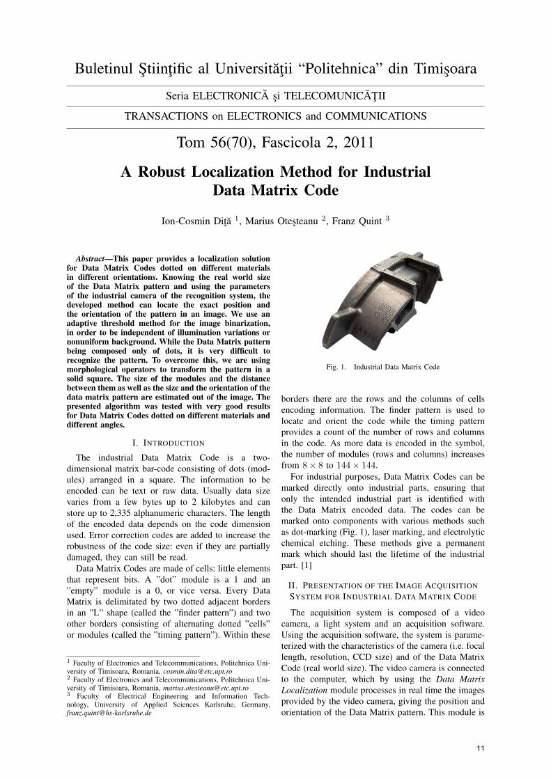
Abstract—This paper provides a localization solutionfor Data Matrix Codes dotted on different materialsin different orientations. Knowing the real world sizeof the Data Matrix pattern and using the parametersof the industrial camera of the recognition system, thedeveloped method can locate the exact position andthe orientation of the pattern in an image. We use anadaptive threshold method for the image binarization,in order to be independent of illumination variations ornonuniform background. While the Data Matrix patternbeing composed only of dots, it is very difficult torecognize the pattern. To overcome this, we are usingmorphological operators to transform the pattern in asolid square. The size of the modules and the distancebetween them as well as the size and the orientation of thedata matrix pattern are estimated out of the image. Thepresented algorithm was tested with very good resultsfor Data Matrix Codes dotted on different materials anddifferent angles.
I. INTRODUCTION
The industrial Data Matrix Code is a two-dimensional matrix bar-code consisting of dots (mod-ules) arranged in a square. The information to beencoded can be text or raw data. Usually data sizevaries from a few bytes up to 2 kilobytes and canstore up to 2,335 alphanumeric characters. The lengthof the encoded data depends on the code dimensionused. Error correction codes are added to increase therobustness of the code size: even if they are partiallydamaged, they can still be read.
Data Matrix Codes are made of cells: little elementsthat represent bits. A ”dot” module is a 1 and an”empty” module is a 0, or vice versa. Every DataMatrix is delimitated by two dotted adjacent bordersin an ”L” shape (called the ”finder pattern”) and twoother borders consisting of alternating dotted ”cells”or modules (called the ”timing pattern”). Within these
1 Faculty of Electronics and Telecommunications, Politehnica Uni-versity of Timisoara, Romania, [email protected] Faculty of Electronics and Telecommunications, Politehnica Uni-versity of Timisoara, Romania, [email protected] Faculty of Electrical Engineering and Information Tech-nology, University of Applied Sciences Karlsruhe, Germany,[email protected]
Fig. 1. Industrial Data Matrix Code
borders there are the rows and the columns of cellsencoding information. The finder pattern is used tolocate and orient the code while the timing patternprovides a count of the number of rows and columnsin the code. As more data is encoded in the symbol,the number of modules (rows and columns) increasesfrom 8× 8 to 144× 144.
For industrial purposes, Data Matrix Codes can bemarked directly onto industrial parts, ensuring thatonly the intended industrial part is identified withthe Data Matrix encoded data. The codes can bemarked onto components with various methods suchas dot-marking (Fig. 1), laser marking, and electrolyticchemical etching. These methods give a permanentmark which should last the lifetime of the industrialpart. [1]
II. PRESENTATION OF THE IMAGE ACQUISITIONSYSTEM FOR INDUSTRIAL DATA MATRIX CODE
The acquisition system is composed of a videocamera, a light system and an acquisition software.Using the acquisition software, the system is parame-terized with the characteristics of the camera (i.e. focallength, resolution, CCD size) and of the Data MatrixCode (real world size). The video camera is connectedto the computer, which by using the Data MatrixLocalization module processes in real time the imagesprovided by the video camera, giving the position andorientation of the Data Matrix pattern. This module is
11

connected to the Video Interface and the Data MatrixScanning, as is showed in Fig. 2. The light is mountedon camera body and creates a 45o angle with the DataMatrix Code surface. In [2] is explained why is taken a45o angle between the light system and the code. Nextwe introduce very briefly the Video Interface module.
Data Matrix Scanning
Data Matrix Localization
Video Interface
Video Camera
Fig. 2. The block diagram of the acquisition system
types of cameras and different sizes of Data Matrix Pattern.Because this system is used in industrial environment, we canchoose few characteristics about video camera like: the CCDsize, the resolution and the focal length of lenses that areused, and other information about the real world code sizeand the distance between camera and the code. Using theseinformation we can compute the size in pixels of Data Matrixcode, this computation is just an estimation for the size, buthelps us to restrict the area of searching for Data Matrix code.Of course this calculation is not accurate, but for that reasonwe take a tolerance given by a constant chosen by the operator.Using next equations we can compute the size of image inpixels (I) as:
B = b · Gg, (1)
I = B2 · w · hs
, (2)
where:G is the real world Data Matrix size (cm),B is the size of Data Matrix projection on CCD,g the distance between code and video camera,b is the focal length of lenses,s is the size of CCD,w is the vertical resolution of CCD,h is the horizontal resolution of CCD.
B. Modules scanning
The modules scanning block takes the information with thecoordinates of the corners and the code orientation and scansinside of the code in few steps:• computation of the distance between modules,• the finder pattern recognition,• modules scanning,For computation the general distance between modules, an-
alyzes the distance between the each module and 4 neighborsof it, the results being written in a matrix of distances. Afterall modules are queried, all data are stored and the pick ofthe histogram is the general distance between modules. Thefinder pattern composed from two dotted adjacent borders inan ”L” shape. To recognize this pattern, using the distancebetween dots and the code orientation, all 4 corners al queriedfor neighbors in two direction to outside displaced with 90o.The corner with two neighbors is the main corner and theother two adjacent corners are the others corners of the finder
pattern. The modules scanning starts from the main cornerand using the modules distance and the orientation angle ofthe code, searches in rows and columns for each dots creatinga matrix of coordinates.
III. DATA MATRIX LOCALIZATION
The localization of region of interest (ROI) is an importantstage in operation of image processing. To identify the correctposition of ROI, we have to use some information about theshape of Data Matrix pattern.
Shape side
Shap
e s
ide
90o
Fig. 3. Data Matrix code
We know that the pattern is a square and also we knowthe estimated size of the pattern sides, so the first conditionfor the searched object is the sides of the pattern should beequal. The second condition is the pattern size to be equal topredicted size of the code, and the third condition is all theangles of the geometric shape of the pattern to be equal with90o.
Image acquisition
RGB to Gray
Image sub-sampling
Adaptive thresholding
Dilate & Erode
Extracting the region of interest (ROI)
Corners position Orientation angle
Min. Axis Max. Axis
Extremes & Corners Angles
Predicted perimeter
Angles&Sides precision
Fig. 4. Data Matrix localization process
If we follow the block diagram of the localization system(Figure 4), we can see that a RGB image is captured and
Fig. 2. The block diagram of the acquisition system
III. VIDEO INTERFACE
The interface is the direct connection between userand the acquisition system, displaying the result of theData Matrix scanning. This module also allows us toparameterize the acquisition system for different typesof cameras and different sizes of Data Matrix pattern.Because this system is used in industrial environment,we can choose few characteristics about video cameralike: the CCD size, the CCD resolution, the focallength of lenses that are used, information about thereal world code size and the approximate distancebetween camera and the code. Using these informationwe can compute the size in pixels of the Data MatrixCode. This computation is an estimation for the size,helping us to restrict the area of searching for theData Matrix Code. Using equations (1) and (2), wecan compute the size of the image in pixels (I) as:
B = b · Gg, (1)
I = B2 · w · hs
, (2)
where:G is the real world Data Matrix size (cm),B is the size of Data Matrix projection on CCD,g the distance between code and video camera
(cm),b is the distance between sensor and optical
center of the lens, approximate focal length(in case of focus to ∞),
s is the diagonal length of the CCD (cm),w is the vertical number of pixels of the CCD,h is the horizontal number of pixels of the
CCD.
IV. DATA MATRIX LOCALIZATION
The pre-processing stage is used to locate the DataMatrix pattern, without having interest in image de-tails. To identify the correct position of ROI, we haveto use some information about the shape of the DataMatrix pattern.
Data Matrix Scanning
Data Matrix Localization
Video Interface
Video Camera
Fig. 2. The block diagram of the acquisition system
types of cameras and different sizes of Data Matrix Pattern.Because this system is used in industrial environment, we canchoose few characteristics about video camera like: the CCDsize, the resolution and the focal length of lenses that areused, and other information about the real world code sizeand the distance between camera and the code. Using theseinformation we can compute the size in pixels of Data Matrixcode, this computation is just an estimation for the size, buthelps us to restrict the area of searching for Data Matrix code.Of course this calculation is not accurate, but for that reasonwe take a tolerance given by a constant chosen by the operator.Using next equations we can compute the size of image inpixels (I) as:
B = b · Gg, (1)
I = B2 · w · hs
, (2)
where:G is the real world Data Matrix size (cm),B is the size of Data Matrix projection on CCD,g the distance between code and video camera,b is the focal length of lenses,s is the size of CCD,w is the vertical resolution of CCD,h is the horizontal resolution of CCD.
B. Modules scanning
The modules scanning block takes the information with thecoordinates of the corners and the code orientation and scansinside of the code in few steps:• computation of the distance between modules,• the finder pattern recognition,• modules scanning,For computation the general distance between modules, an-
alyzes the distance between the each module and 4 neighborsof it, the results being written in a matrix of distances. Afterall modules are queried, all data are stored and the pick ofthe histogram is the general distance between modules. Thefinder pattern composed from two dotted adjacent borders inan ”L” shape. To recognize this pattern, using the distancebetween dots and the code orientation, all 4 corners al queriedfor neighbors in two direction to outside displaced with 90o.The corner with two neighbors is the main corner and theother two adjacent corners are the others corners of the finder
pattern. The modules scanning starts from the main cornerand using the modules distance and the orientation angle ofthe code, searches in rows and columns for each dots creatinga matrix of coordinates.
III. DATA MATRIX LOCALIZATION
The localization of region of interest (ROI) is an importantstage in operation of image processing. To identify the correctposition of ROI, we have to use some information about theshape of Data Matrix pattern.
Shape side
Shap
e s
ide
90o
Fig. 3. Data Matrix code
We know that the pattern is a square and also we knowthe estimated size of the pattern sides, so the first conditionfor the searched object is the sides of the pattern should beequal. The second condition is the pattern size to be equal topredicted size of the code, and the third condition is all theangles of the geometric shape of the pattern to be equal with90o.
Image acquisition
RGB to Gray
Image sub-sampling
Adaptive thresholding
Dilate & Erode
Extracting the region of interest (ROI)
Corners position Orientation angle
Min. Axis Max. Axis
Extremes & Corners Angles
Predicted perimeter
Angles&Sides precision
Fig. 4. Data Matrix localization process
If we follow the block diagram of the localization system(Figure 4), we can see that a RGB image is captured and
Fig. 3. Data Matrix localization process
If we follow the block diagram of the localizationsystem (Fig. 3), we can see that an image is capturedand is sub-sampled using a Sample ratio. If a highSample ratio is chosen, the image is more decreasedand the pre-processing speed is increased, that being agoal for the system. But on the other hand, the objectcharacteristics are considerably reduced. Because ofthat, the Sample ratio is chosen manually by theoperator, depending by the real world size of thepattern.
The image is thresholded using an adaptive thresh-old level [3]. Depending by the estimated patternsize in pixels, the Gray image is divided in regions,each region being equal with the estimated size inpixels of the code, Fig. 4. The number of region isround( Image size
Estimated pattern size ). Using the Otsu method [4]for each region a local threshold level is computed.Otsus method searches for the threshold that mini-mizes the intra-class variance which is defined as theweighted sum of variances of the two classes, equation3.
σ2W (t) =Wb(t) · σ2
b (t) +Wf (t) · σ2f (t), (3)
where Wb,Wf denote the probabilities of the twoclasses separated by a threshold t, and σ2
b , σ2f denote
the variances of these classes. Otsu has proven thatminimizing the intra-class variance is the same asmaximizing interclass variance:
σ2B(t) = σ2−σ2
W (t) =Wb(t)·Wf (t)·(µb(t)−µf (t))2,
(4)which is expressed in terms of class probabilitiesWb,Wf and class means µb, µf , which in turn canbe updated iteratively. We maximize formula 4 to get
12

the Otsu’s threshold. The procedures of Otsu’s methodcan be depicted as follows: [5]• It computes the histogram and the probabilities
of each intensity value,• Sets the initial values of Wb(0),Wf (0) andµb(0), µf (0),
• Loops for all possible thresholds t,• Updates Wb(t),Wf (t) and µb(t), µf (t),• Computes σ2
B(t) and chooses the threshold t∗
corresponding to the maximum of σ2B(t).
converted in Gray with 8 bit, after that is sub-sampled usinga sample ratio. The pre-processing stage is used to locate theData Matrix pattern, without to have interest in image details,because of that the input image is considerably decreased. Ifa high Sample ratio is chosen, the image is more decreasedand the pre-processing speed is increased, that is a goal forthe system, but on the other hand the object characteristicsare considerably reduced. Because of that, the sample ratiois chosen after more tests, the right value taken being themaximum value when the object is still recognized. The imageis thresholded using an adaptive threshold level like in [3],depending by the estimated pattern size in pixels, methodimplemented special for Data Matrix images. The Gray imageis divided in more parts equal with the estimated size inpixels of the code and using the Otsu [4] method is chosena threshold level which minimizes the inter-classes variancebetween withe and black pixels, for each region from dividedimage is calculated a global threshold level and using all valuesis made a matrix local threshold levels like in Image 5.
σ2W =Wb · σ2
b +Wf · σ2f , (3)
σ2B = σ2 − σ2
W =Wb · (µb − µ)2 +Wf · (µf − µ)2=Wb ·Wf · (µb − µf )
2,(4)
where:µ = Wb · µb +Wf · µf ,σb, σf - are the gray variations coresponding to sameintervals,Wb,Wf - represent the probability density of back-ground and foreground pixels,µb, µf - represent the ponderate average of pixelslevels from background and foreground.
th1 th2 th3 th4
th5 th6 th7 th8
th9 th10 th11 th12
Fig. 5. Local threshold levels
Th =
th1 th2 th3 th4th5 th6 th7 th8th9 th10 th11 th12
(5)
=⇒
th1 · · · thw... · · ·
...th(w−1)·h · · · thw·h
(6)
Using bilinear interpolation method [5], the local thresholdlevel matrix is extended to a matrix of threshold levels of the
size of the image. One interpolated value is calculated usingthe weighted average of four neighbors values located on thesampling grid of input matrix, using the next equation:
f(x,y) = (1− α) · (1− β) · f(|x|,|y|)++α · (1− β) · f(|x|+1,|y|) + (1− α) · β · f(|x|,|y|+1)+
+α · β · f(|x|+1,|y|+1),
(7)
α and β are the fractional part of x and y coordinates,Counting the the twos values 1 and 0 from image, we
can estimate the level of the background. It is preferable thebackground to be black (0) and the foreground to be withe(1), this condition is useful for the next stages from imageprocessing process. If this condition is not accomplished,automatic the image is negatived [5] with the relation.
Imgneg = Lmax − Img,Lmax = 1. for binar image
(8)
After that, each pixel from gray image is thresholded, usingone threshold level from extended matrix of adaptive thresholdlevels, using the next relation of cases [5].
BW =
1, for Img ≥ thx ;0, for Img < thx . (9)
Using the adaptive threshold level method, the light vari-ation in the image are reduced creating a binary image withuniform background. The searched object being created frommodules is harder to identify the position, because in imagealso it is noise, light spots, or other objects. To recognizethe Data Matrix without error, the code shape should beseen like a square not like matrix of points. For that, usingthe morphological dilate operation, each module is dilated inorder to fill the empty spaces between modules. The structuralelement can be considered like a disk with a Strel Ratio pixelsradius, this value is chosen depending the pixels between twomodules.
Dilate
Fig. 6. Morphological Dilate Operation
Dilating a set of elements A using a structural B is the setof points for that the structural element moved with the originin the respectively point it is common points (at least one)with the set A which is dilating [5]. The dilation of a set Ausing the B structural element is defined through equation:
Fig. 4. Local threshold levels
Using all threshold levels is created a matrix of localthreshold levels, relation 5.
Th =
th1 th2 th3 th4th5 th6 th7 th8th9 th10 th11 th12
(5)
=⇒
th1 · · · thw... · · ·
...th(w−1)·h · · · thw·h
(6)
Using bilinear interpolation method [6], the localthreshold level matrix is extended to a matrix of thresh-old levels of the size of the image. One interpolatedvalue is calculated using the weighted average of fourneighbors values located on the sampling grid of inputmatrix, using the next equation:
f(x,y) = (1− α) · (1− β) · f(|x|,|y|)++α · (1− β) · f(|x|+1,|y|) + (1− α) · β · f(|x|,|y|+1)+
+α · β · f(|x|+1,|y|+1),(7)
α and β are the fractional part of x and y coordinates.Each pixel from the gray image is thresholded using
one threshold level from extended matrix of adaptivethreshold levels, showed as in the next relation of cases[6].
BW =
1, for Img ≥ thx ,0, for Img < thx . (8)
Using the adaptive threshold method, a binary imageis created.
For the next stages of image processing, it is de-sirable that the background should be black (level 0)and the foreground to be white (level 1). Since eachData Matrix pattern is surrounded by a quiet zone,there are more background than foreground pixels in
a ROI. Thus, by counting the values of zeros and onesin the ROI, we can find out the current backgroundlevel and, if necessary, we can negate the image tohave a zero-level background [6].
In the image, there can also be noise, light spots, orother objects. Because the searched object is createdonly from modules it is harder to identify its position.To recognize the Data Matrix pattern, the code shapeshould be seen like a square not like a matrix of points.For that, using the morphological dilate operation, theimage is dilated in order to fill the empty spacesbetween modules, Fig. 5. The structural element canbe considered like a disk with a Strel Ratio pixelsradius. This value is chosen depending on numbersof modules.
Dilate
Fig. 5. Morphological Dilate Operation
The dilation process is performed by laying thestructuring element B on the image A and sliding itacross the image in a manner similar to convolution.If one pixel from the structuring element B coincideswith a ’white’ pixel in the image, then it turns theorigin of the structuring element to ’white’ [6]. Let beE an Euclidean space or an integer grid, A a binaryimage in E, and B a structuring element. The dilationof a set A using the B structural element is definedthrough equation:
A⊕B = z ∈ E|(BS)z ∩A 6= ∅, (9)
where Bs denotes the symmetric of B, that is
Bs = x ∈ E| − x ∈ B.The generated effect by the dilation operation is to
expand the objects. All white objects in the image areconnected between, building a square. In the dilatedimage all object are expanded all around with StrelRatio pixels.
Using the erode operation, the objects are resized tothe initial dimension.
Erode
Fig. 6. Morphological Erode Operation
The erosion process is similar to dilation, but weturn pixels to ’black’, not to ’white’. As before, the
13
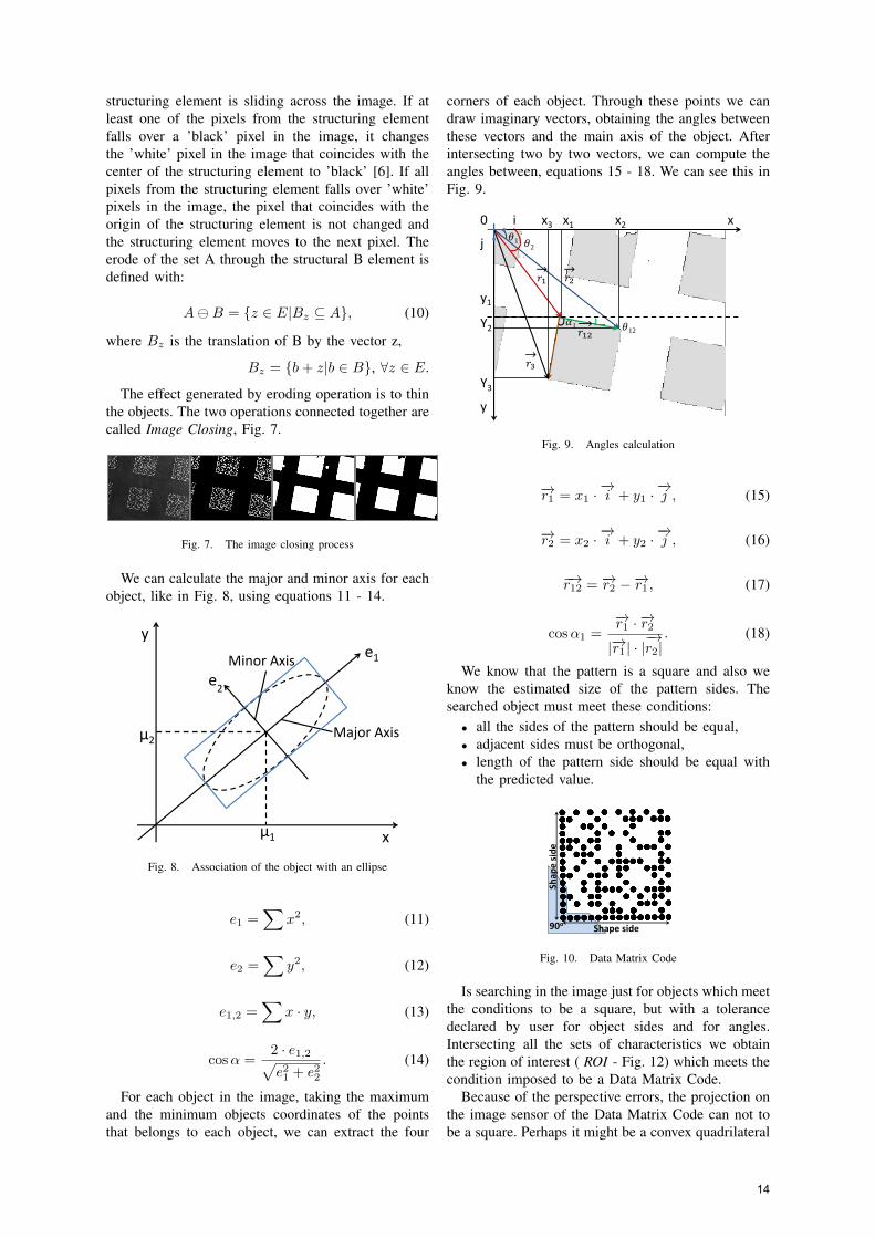
structuring element is sliding across the image. If atleast one of the pixels from the structuring elementfalls over a ’black’ pixel in the image, it changesthe ’white’ pixel in the image that coincides with thecenter of the structuring element to ’black’ [6]. If allpixels from the structuring element falls over ’white’pixels in the image, the pixel that coincides with theorigin of the structuring element is not changed andthe structuring element moves to the next pixel. Theerode of the set A through the structural B element isdefined with:
AB = z ∈ E|Bz ⊆ A, (10)
where Bz is the translation of B by the vector z,
Bz = b+ z|b ∈ B, ∀z ∈ E.
The effect generated by eroding operation is to thinthe objects. The two operations connected together arecalled Image Closing, Fig. 7.
A⊕B = x|Bx ∩A 6= ∅ = (A ∗B| B1 = ∅B2 = B
)C (10)
The generated effect by the dilation operation is to expandthe objects, all white objects in the image are connectedbetween, building a square. In the dilated image all objectare expanded all around with Strel Ratio pixels, because ofthat the objects must be resized to the initial dimension usingthe erode operation, so each group of pixels which looks likea disk with Strel Ratio radius is erased.
Erode
Fig. 7. Morphological Erode Operation
Eroding of a set A through the structured through thestructural B element is the set of points for which the structuralelement is moved with the origin in respectively point isincluded in the set which is eroding [5]. The erode of theset A through the structural B element is defined with:
AB = x|Bx ∩A = (A ∗B| B2 = ∅B1 = B
)C (11)
the effect generated by eroding operation is to thin theobjects, process which is depending by the structural element.The two operations connected together are called image close.
Fig. 8. The image close process
The image being morphological processed, each object fromthe image can considered as a ellipse, thus we can calculatethe major and minor axis for each object, like 9.
m2x =∑
x2, (12)
m2y =∑
y2, (13)
m2xy =∑
x · y, (14)
cosα =2 ·m2xy√m2
2x +m22y
. (15)
e1
e2
y
x
µ2
µ1
Major Axis
Minor Axis
Fig. 9. Association of the object with an ellipse
For each object in the image, taking the maximum andminimum objects coordinates of the points that belongs to eachobject, we can extract the four corners of objects. Throughthese points we can draw imaginary vectors, obtaining theangles between these vectors and the main axis of the image,after that intersecting two by two vectors we can compute theangles obtained by these. We can see this in figure 10
0 i x3 x1 x2 x
j
𝑟1
𝑟2
y1
Y2 𝑟12
𝑟3
Y3
y
𝜃1 𝜃2
𝜃12 𝛼1
Fig. 10. Angles calculation
−→r1 = x1 ·−→i + y1 ·
−→j , (16)
−→r2 = x2 ·−→i + y2 ·
−→j , (17)
−→r12 = −→r2 −−→r1 , (18)
tan θ1 =y1x1, tan θ2 =
y2x2, tan θ12 =
y2 − y1x2 − x1
, (19)
cosα1 =−→r1 · −→r2|−→r1 | · |
−→r2|. (20)
Fig. 7. The image closing process
We can calculate the major and minor axis for eachobject, like in Fig. 8, using equations 11 - 14.
A⊕B = x|Bx ∩A 6= ∅ = (A ∗B| B1 = ∅B2 = B
)C (10)
The generated effect by the dilation operation is to expandthe objects, all white objects in the image are connectedbetween, building a square. In the dilated image all objectare expanded all around with Strel Ratio pixels, because ofthat the objects must be resized to the initial dimension usingthe erode operation, so each group of pixels which looks likea disk with Strel Ratio radius is erased.
Erode
Fig. 7. Morphological Erode Operation
Eroding of a set A through the structured through thestructural B element is the set of points for which the structuralelement is moved with the origin in respectively point isincluded in the set which is eroding [5]. The erode of theset A through the structural B element is defined with:
AB = x|Bx ∩A = (A ∗B| B2 = ∅B1 = B
)C (11)
the effect generated by eroding operation is to thin theobjects, process which is depending by the structural element.The two operations connected together are called image close.
Fig. 8. The image close process
The image being morphological processed, each object fromthe image can considered as a ellipse, thus we can calculatethe major and minor axis for each object, like 9.
m2x =∑
x2, (12)
m2y =∑
y2, (13)
m2xy =∑
x · y, (14)
cosα =2 ·m2xy√m2
2x +m22y
. (15)
e1
e2
y
x
µ2
µ1
Major Axis
Minor Axis
Fig. 9. Association of the object with an ellipse
For each object in the image, taking the maximum andminimum objects coordinates of the points that belongs to eachobject, we can extract the four corners of objects. Throughthese points we can draw imaginary vectors, obtaining theangles between these vectors and the main axis of the image,after that intersecting two by two vectors we can compute theangles obtained by these. We can see this in figure 10
0 i x3 x1 x2 x
j
𝑟1
𝑟2
y1
Y2 𝑟12
𝑟3
Y3
y
𝜃1 𝜃2
𝜃12 𝛼1
Fig. 10. Angles calculation
−→r1 = x1 ·−→i + y1 ·
−→j , (16)
−→r2 = x2 ·−→i + y2 ·
−→j , (17)
−→r12 = −→r2 −−→r1 , (18)
tan θ1 =y1x1, tan θ2 =
y2x2, tan θ12 =
y2 − y1x2 − x1
, (19)
cosα1 =−→r1 · −→r2|−→r1 | · |
−→r2|. (20)
Fig. 8. Association of the object with an ellipse
e1 =∑
x2, (11)
e2 =∑
y2, (12)
e1,2 =∑
x · y, (13)
cosα =2 · e1,2√e21 + e22
. (14)
For each object in the image, taking the maximumand the minimum objects coordinates of the pointsthat belongs to each object, we can extract the four
corners of each object. Through these points we candraw imaginary vectors, obtaining the angles betweenthese vectors and the main axis of the object. Afterintersecting two by two vectors, we can compute theangles between, equations 15 - 18. We can see this inFig. 9.
A⊕B = x|Bx ∩A 6= ∅ = (A ∗B| B1 = ∅B2 = B
)C (10)
The generated effect by the dilation operation is to expandthe objects, all white objects in the image are connectedbetween, building a square. In the dilated image all objectare expanded all around with Strel Ratio pixels, because ofthat the objects must be resized to the initial dimension usingthe erode operation, so each group of pixels which looks likea disk with Strel Ratio radius is erased.
Erode
Fig. 7. Morphological Erode Operation
Eroding of a set A through the structured through thestructural B element is the set of points for which the structuralelement is moved with the origin in respectively point isincluded in the set which is eroding [5]. The erode of theset A through the structural B element is defined with:
AB = x|Bx ∩A = (A ∗B| B2 = ∅B1 = B
)C (11)
the effect generated by eroding operation is to thin theobjects, process which is depending by the structural element.The two operations connected together are called image close.
Fig. 8. The image close process
The image being morphological processed, each object fromthe image can considered as a ellipse, thus we can calculatethe major and minor axis for each object, like 9.
m2x =∑
x2, (12)
m2y =∑
y2, (13)
m2xy =∑
x · y, (14)
cosα =2 ·m2xy√m2
2x +m22y
. (15)
e1
e2
y
x
µ2
µ1
Major Axis
Minor Axis
Fig. 9. Association of the object with an ellipse
For each object in the image, taking the maximum andminimum objects coordinates of the points that belongs to eachobject, we can extract the four corners of objects. Throughthese points we can draw imaginary vectors, obtaining theangles between these vectors and the main axis of the image,after that intersecting two by two vectors we can compute theangles obtained by these. We can see this in figure 10
0 i x3 x1 x2 x
j
𝑟1
𝑟2
y1
Y2 𝑟12
𝑟3
Y3
y
𝜃1 𝜃2
𝜃12 𝛼1
Fig. 10. Angles calculation
−→r1 = x1 ·−→i + y1 ·
−→j , (16)
−→r2 = x2 ·−→i + y2 ·
−→j , (17)
−→r12 = −→r2 −−→r1 , (18)
tan θ1 =y1x1, tan θ2 =
y2x2, tan θ12 =
y2 − y1x2 − x1
, (19)
cosα1 =−→r1 · −→r2|−→r1 | · |
−→r2|. (20)
Fig. 9. Angles calculation
−→r1 = x1 ·−→i + y1 ·
−→j , (15)
−→r2 = x2 ·−→i + y2 ·
−→j , (16)
−→r12 = −→r2 −−→r1 , (17)
cosα1 =−→r1 · −→r2|−→r1 | · |
−→r2|. (18)
We know that the pattern is a square and also weknow the estimated size of the pattern sides. Thesearched object must meet these conditions:• all the sides of the pattern should be equal,• adjacent sides must be orthogonal,• length of the pattern side should be equal with
the predicted value.
Data Matrix Scanning
Data Matrix Localization
Video Interface
Video Camera
Fig. 2. The block diagram of the acquisition system
types of cameras and different sizes of Data Matrix Pattern.Because this system is used in industrial environment, we canchoose few characteristics about video camera like: the CCDsize, the resolution and the focal length of lenses that areused, and other information about the real world code sizeand the distance between camera and the code. Using theseinformation we can compute the size in pixels of Data Matrixcode, this computation is just an estimation for the size, buthelps us to restrict the area of searching for Data Matrix code.Of course this calculation is not accurate, but for that reasonwe take a tolerance given by a constant chosen by the operator.Using next equations we can compute the size of image inpixels (I) as:
B = b · Gg, (1)
I = B2 · w · hs
, (2)
where:G is the real world Data Matrix size (cm),B is the size of Data Matrix projection on CCD,g the distance between code and video camera,b is the focal length of lenses,s is the size of CCD,w is the vertical resolution of CCD,h is the horizontal resolution of CCD.
B. Modules scanning
The modules scanning block takes the information with thecoordinates of the corners and the code orientation and scansinside of the code in few steps:• computation of the distance between modules,• the finder pattern recognition,• modules scanning,For computation the general distance between modules, an-
alyzes the distance between the each module and 4 neighborsof it, the results being written in a matrix of distances. Afterall modules are queried, all data are stored and the pick ofthe histogram is the general distance between modules. Thefinder pattern composed from two dotted adjacent borders inan ”L” shape. To recognize this pattern, using the distancebetween dots and the code orientation, all 4 corners al queriedfor neighbors in two direction to outside displaced with 90o.The corner with two neighbors is the main corner and theother two adjacent corners are the others corners of the finder
pattern. The modules scanning starts from the main cornerand using the modules distance and the orientation angle ofthe code, searches in rows and columns for each dots creatinga matrix of coordinates.
III. DATA MATRIX LOCALIZATION
The localization of region of interest (ROI) is an importantstage in operation of image processing. To identify the correctposition of ROI, we have to use some information about theshape of Data Matrix pattern.
Shape side
Shap
e s
ide
90o
Fig. 3. Data Matrix code
We know that the pattern is a square and also we knowthe estimated size of the pattern sides, so the first conditionfor the searched object is the sides of the pattern should beequal. The second condition is the pattern size to be equal topredicted size of the code, and the third condition is all theangles of the geometric shape of the pattern to be equal with90o.
Image acquisition
RGB to Gray
Image sub-sampling
Adaptive thresholding
Dilate & Erode
Extracting the region of interest (ROI)
Corners position Orientation angle
Min. Axis Max. Axis
Extremes & Corners Angles
Predicted perimeter
Angles&Sides precision
Fig. 4. Data Matrix localization process
If we follow the block diagram of the localization system(Figure 4), we can see that a RGB image is captured and
Fig. 10. Data Matrix Code
Is searching in the image just for objects which meetthe conditions to be a square, but with a tolerancedeclared by user for object sides and for angles.Intersecting all the sets of characteristics we obtainthe region of interest ( ROI - Fig. 12) which meets thecondition imposed to be a Data Matrix Code.
Because of the perspective errors, the projection onthe image sensor of the Data Matrix Code can not tobe a square. Perhaps it might be a convex quadrilateral
14

as in Fig. 11 and, to overcame this we use a tolerancefor angles and for sides.
Is calling on all the angles the major and minor axis, andis searching in the image just the objects which meet the nextconditions but with a tolerance declared by user for objectsides and angles. If Obj is the set of all objects in the imagethen we now the corners angles, major axis and minor axisthen:
Objang is the corners angles setObjmaj is the major axis setObjmin is minor axis set
I1 = Objmaj ∩ (Objmin ± SideTolerance) (21)
I2 = Objmaj ∩ (EstimatedSide± SideTolerance) (22)
I3 = Objmin ∩ (EstimatedSide± SideTolerance) (23)
I4 = Objang ∩ (90o ±AngleTolerance) (24)
ROI = I1 ∩ I2 ∩ I3 ∩ I4 (25)
Intersecting all the sets of characteristics we obtain theregion of interest which meets the condition imposed to be likea Data Matrix code. It is used this tolerance for angles and forsides, because we don’t know the position of the video camerato the code, and because of the perspective errors it is possiblethe projection of the Data Matrix code on the image sensornot to be a square, perhaps might be a convex quadrilateral asin Figure ??.
Major Axis
Min
or
Axi
s
α1
α2 α3
Fig. 11. Data Matrix code - Perspective error
If the code is dotted on cylindrical or spherical objects,or even if the pattern has a perspective error because thevideo camera lenses are not the best quality, is taken a safetytolerance for Data Matrix pattern helping in that way therecognize video system to locate the right position of the code.
IV. CONCLUSION
The localization of region of interest (ROI) is an importantstage in operation of the image processing process for DataMatrix Reader. Using adaptive threshold level for imagebinarization depending by the pattern size, the backgroundof the image is constant, the differences of gray levels beingreduced. Closing the image using the morphological operators
ROI
Corner1
Corner4 Corner3
Corner2
Fig. 12. Region of interest - Data Matrix
dilate and erode helps to recognize the code position, thus therecognition system being more stabile and accurate. Using thescanner system for industrial use, we know some characteris-tics about the code, because it we can define a shape of thepattern, thus the searching area being reduced. This stage ofimage pre-processing it works in real time with good resultsfor materials that have the property of light reflection, thetests being executed in an environment with one light sourcemounted on 45o to the code surface. In the cases when plasticmaterials were tested, it is hard to recognize the position ofData Matrix pattern in the image, because the light reflectionis to small or null for white color.
V. ACKNOWLEDGMENT
This work was partially supported by the strategic grantPOSDRU 6/1.5/S/13, (2008) of the Ministry of Labour, Familyand Social Protection, Romania, co-financed by the EuropeanSocial Fund Investing in People.
REFERENCES
[1] INTERNATIONAL STANDARD, “Information technology — Interna-tional symbology specification — Data matrix,” 2000-05-01.
[2] Dita Ion-Cosmin and Otesteanu Marius, Eds., Factors that Influence theImage Acquisition of Direct Marking Data Matrix Code, Serbia, Belgrade,2009.
[3] Ye Zhang, Hongsong Qu, and Yanjie Wang, “Adaptive Image Segmenta-tion Based on Fast Thresholding and Image Merging: Artificial Realityand Telexistence–Workshops, 2006. ICAT ’06. 16th International Con-ference on: Artificial Reality and Telexistence–Workshops, 2006. ICAT’06. 16th International Conference on DOI - 10.1109/ICAT.2006.32,”Artificial Reality and Telexistence–Workshops, 2006. ICAT ’06. 16thInternational Conference on, pp. 308–311, 2006.
[4] N. Otsu, “A Threshold Selection Method from Gray-Level Histograms:Systems, Man and Cybernetics, IEEE Transactions on,” Systems, Manand Cybernetics, IEEE Transactions on, vol. 9, no. 1, pp. 62–66, 1979.
[5] Vasile Gui, Prelucrarea numerica a imaginii.
Fig. 11. Data Matrix Code - Perspective error
Is calling on all the angles the major and minor axis, andis searching in the image just the objects which meet the nextconditions but with a tolerance declared by user for objectsides and angles. If Obj is the set of all objects in the imagethen we now the corners angles, major axis and minor axisthen:
Objang is the corners angles setObjmaj is the major axis setObjmin is minor axis set
I1 = Objmaj ∩ (Objmin ± SideTolerance) (21)
I2 = Objmaj ∩ (EstimatedSide± SideTolerance) (22)
I3 = Objmin ∩ (EstimatedSide± SideTolerance) (23)
I4 = Objang ∩ (90o ±AngleTolerance) (24)
ROI = I1 ∩ I2 ∩ I3 ∩ I4 (25)
Intersecting all the sets of characteristics we obtain theregion of interest which meets the condition imposed to be likea Data Matrix code. It is used this tolerance for angles and forsides, because we don’t know the position of the video camerato the code, and because of the perspective errors it is possiblethe projection of the Data Matrix code on the image sensornot to be a square, perhaps might be a convex quadrilateral asin Figure ??.
Major Axis
Min
or
Axi
s
α1
α2 α3
Fig. 11. Data Matrix code - Perspective error
If the code is dotted on cylindrical or spherical objects,or even if the pattern has a perspective error because thevideo camera lenses are not the best quality, is taken a safetytolerance for Data Matrix pattern helping in that way therecognize video system to locate the right position of the code.
IV. CONCLUSION
The localization of region of interest (ROI) is an importantstage in operation of the image processing process for DataMatrix Reader. Using adaptive threshold level for imagebinarization depending by the pattern size, the backgroundof the image is constant, the differences of gray levels beingreduced. Closing the image using the morphological operators
ROI
Corner1
Corner4 Corner3
Corner2
Fig. 12. Region of interest - Data Matrix
dilate and erode helps to recognize the code position, thus therecognition system being more stabile and accurate. Using thescanner system for industrial use, we know some characteris-tics about the code, because it we can define a shape of thepattern, thus the searching area being reduced. This stage ofimage pre-processing it works in real time with good resultsfor materials that have the property of light reflection, thetests being executed in an environment with one light sourcemounted on 45o to the code surface. In the cases when plasticmaterials were tested, it is hard to recognize the position ofData Matrix pattern in the image, because the light reflectionis to small or null for white color.
V. ACKNOWLEDGMENT
This work was partially supported by the strategic grantPOSDRU 6/1.5/S/13, (2008) of the Ministry of Labour, Familyand Social Protection, Romania, co-financed by the EuropeanSocial Fund Investing in People.
REFERENCES
[1] INTERNATIONAL STANDARD, “Information technology — Interna-tional symbology specification — Data matrix,” 2000-05-01.
[2] Dita Ion-Cosmin and Otesteanu Marius, Eds., Factors that Influence theImage Acquisition of Direct Marking Data Matrix Code, Serbia, Belgrade,2009.
[3] Ye Zhang, Hongsong Qu, and Yanjie Wang, “Adaptive Image Segmenta-tion Based on Fast Thresholding and Image Merging: Artificial Realityand Telexistence–Workshops, 2006. ICAT ’06. 16th International Con-ference on: Artificial Reality and Telexistence–Workshops, 2006. ICAT’06. 16th International Conference on DOI - 10.1109/ICAT.2006.32,”Artificial Reality and Telexistence–Workshops, 2006. ICAT ’06. 16thInternational Conference on, pp. 308–311, 2006.
[4] N. Otsu, “A Threshold Selection Method from Gray-Level Histograms:Systems, Man and Cybernetics, IEEE Transactions on,” Systems, Manand Cybernetics, IEEE Transactions on, vol. 9, no. 1, pp. 62–66, 1979.
[5] Vasile Gui, Prelucrarea numerica a imaginii.
Fig. 12. Region of interest - Data Matrix Code
V. DATA MATRIX SCANNING
The Data Matrix scanning block takes the informa-tion with the coordinates of the corners and the codeorientation and scans inside of the code in few steps:• computation of the distance between modules,• the Finder pattern recognition,• modules scanning,For computation of the general distance between
modules, it analyzes the distance between each moduleand 4 neighbors of it. The results are written in amatrix of distances. After all modules are queried, alldata are stored and the peak of the histogram is thedistance between modules.
The finder pattern is composed from two dottedadjacent borders in a ”L” shape. To recognize thispattern, using the distance between dots and the codeorientation, all 4 corners are queried to outside forneighbors in two direction displaced with 90o. Thecorner with two neighbors is the main corner and theother two adjacent corners are the others corners ofthe finder pattern.
For the modules scanning, it starts to scan from themain corner using the modules distance and the ori-entation angle of the code. It is searching in rows andcolumns for each dot creating a matrix of coordinatesof dotted and un-dotted modules.
VI. CONCLUSION
The localization of region of interest (ROI) is animportant stage in operation of the image process-ing process for Data Matrix Reader. Using adaptivethreshold level for image binarization, the differencesof gray levels are reduced. Closing the image usingthe morphological operators dilate and erode helps to
recognize the code position. Thus the recognition sys-tem being more accurate. Because of the Localizationsystem is used for industrial Data Matrix Code recog-nition, the characteristics of the pattern are known.Thus it can be define a shape of the pattern and inthat way the searching area is reduced. In the nextfigures (Figures: 13 - 16), we give four examples oftests on different types of Datas Matrix Codes.
In Fig. 13, the code is dotted on glossy copper, thesize of the pattern is 2 cm and in Fig. 14, the codeis dotted on shiny aluminum, the size of the patternbeing 1,6 cm.
DataMatrix detected:angle=17
A(178.5, 77.5)B(236.5, 93.5)
C(219.5, 151.5)
D(162.5, 132.5)
Fig. 13. Glossy copper, pattern size 2 cm
DataMatrix detected:angle=45
A(88.5, 52.5)
B(118.5, 76.5)
C(85.5, 108.5)
D(55.5, 78.5)
angle=45A(88.5, 52.5)
B(118.5, 76.5)
C(85.5, 108.5)
D(55.5, 78.5)
angle=45A(88.5, 52.5)
B(118.5, 76.5)
C(85.5, 108.5)
D(55.5, 78.5)
Fig. 14. Shiny aluminum, pattern size 1.6 cm
In Figures 13 and 14, we can see that the real worldsize of the code and the number of modules are notimportant for the localization. The code is successfullylocated in both cases.
In Fig. 15, the code is dotted on iron with rust spots,the size of the pattern is 1,6 cm and in Fig. 16, thecode is dotted on metals coated with texture, the sizeof the pattern being 2 cm.
DataMatrix detected:angle=26
A(31.5, 85.5)B(60.5, 100.5)
C(35.5, 139.5)D(10.5, 130.5)
Fig. 15. Iron with rust spots, pattern size 1.6 cm
In these two cases we can see that the backgroundof the code is not important in the image localizationprocess. In both cases the spots of rust and paintdoesn’t affect the localization system.
The tests are executed in an environment with onelight source mounted on 45o to the code surface. This
15

DataMatrix detected:angle=63
A(82.5, 27.5)
B(113.5, 85.5)
C(61.5, 109.5)
D(27.5, 51.5)
Fig. 16. Metals coated with texture, pattern size 2 cm
stage, of image pre-processing, works in real time withgood results for materials that have the property oflight reflection. In the cases when plastic materialswere tested, it is hard to recognize the position in theimage of Data Matrix pattern. Because in these casesthe light reflection is to small or null especially forwhite color.
VII. ACKNOWLEDGMENT
This work was partially supported by the strategicgrant POSDRU 6/1.5/S/13, (2008) of the Ministry ofLabour, Family and Social Protection, Romania, co-financed by the European Social Fund Investing inPeople.
REFERENCES
[1] INTERNATIONAL STANDARD, “Information technology —International symbology specification — Data matrix,” 2000-05-01.
[2] Dita Ion-Cosmin and Otesteanu Marius, Eds., Factors thatInfluence the Image Acquisition of Direct Marking Data MatrixCode, vol. TELFOR 2009, Serbia, Belgrade, 2009.
[3] Ye Zhang, Hongsong Qu, and Yanjie Wang, “Adaptive ImageSegmentation Based on Fast Thresholding and Image Merging,”Artificial Reality and Telexistence–Workshops, 2006. ICAT ’06.16th International Conference on, pp. 308–311, 2006.
[4] N. Otsu, “A Threshold Selection Method from Gray-LevelHistograms,” IEEE Transactions on Systems, Man and Cyber-netics, DOI - 10.1109/TSMC.1979.4310076 (Systems, Man andCybernetics, IEEE Transactions on), vol. 9, no. 1, pp. 62–66,1979.
[5] L. W. U. Yudong ZHANG, “Fast Document Image BinarizationBased on an Improved Adaptive Otsu’s Method and DestinationWord Accumulation,” vol. JCIS 2011 Vol. 7 (6) : 1886- 1892,2011.
[6] V Gui, D Lacrama, and D Pescaru, Prelucrarea imaginilor.Editura Politehnica Timisoara, 1999.
16
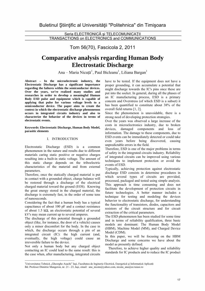
Buletinul Ştiinţific al Universităţii "Politehnica" din Timişoara
Seria ELECTRONICĂ şi TELECOMUNICAŢII TRANSACTIONS on ELECTRONICS and COMMUNICATIONS
Tom 56(70), Fascicola 2, 2011
Comparative analysis regarding Human Body Electrostatic Discharge
Ana – Maria Nicuţă1, Paul Bicleanu1, Liliana Bargan1
1Universitatea Tehnică „Gheorghe Asachi” Iaşi, Facultatea de Inginerie Electrică, Energetică şi Informatică Aplicată Bd. Profesor Dimitrie Mangeron, nr. 21 - 23, Iaşi, email: [email protected], [email protected]
Abstract – In the microelectronic industry, the Electrostatic Discharge has a significant importance regarding the failures within the semiconductor devices. Over the years, we’re realized many studies and researches in order to develop a meaningful Human Body ESD pulse and equipment which is capable of applying that pulse for various voltage levels to a semiconductor device. The paper aims to create the context in which the electrostatic discharge phenomenon occurs in integrated circuits industry and also to characterize the behavior of the devices in terms of electrostatic events. Keywords: Electrostatic Discharge, Human Body Model, parasitic elements
I. INTRODUCTION
Electrostatic Discharge (ESD) is a common phenomenon in the nature and results due to different materials caring static positive or negative charges resulting into a built-in static voltage. The amount of this static charge depends on the triboelectric characteristics of the material and from external parameters. Therefore, once the statically charged material is put in contact with a grounded object, charge balance will be restored through a discharge of the electrical charged material toward the ground (EOS). Knowing the great energy stored in the charged material, the discharge is extremely fast, in the order of some tens of nanoseconds. Considering the fact that a human body has a typical capacitance of about 100 pF and a contact resistance of about 1.5 kΩ, an electrostatic potential of several kV's may mean current up to several amperes. The discharge of this potential through a grounded object (like, for instance, the door of a vehicle) causes only a minor discomfort for the body. In the case in which, the discharge occurs through a pin of an integrated circuit (IC): the high current (and, eventually, the high voltage) could cause an irreversible failure to the device. Not only a human body but any charged object contacting an IC could lead to the same result: this is the case when, after manufacturing, integrated circuits
have to be tested. If the equipment does not have a proper grounding, it can accumulate a potential that might discharge towards the IC's pins once these are put into the socket. In general, during all the phases of an IC manufacturing process, ESD is a primary concern and Overstress (of which ESD is a subset) it has been quantified to constitute about 38% of the overall field returns [1, 2]. Since the phenomenon is unavoidable, there is a strong need of developing protection strategies. Over the years was observed a large increase of the costs in microelectronics industry, due to broken devices, damaged components and loss of information. The damage to these components, due to ESD events can be immediately detected or could take even years before being discovered, causing unpredictable errors in the field. Therefore, ESD is one of the major problems in terms of safety in the integrated circuits industry. Reliability of integrated circuits can be improved using various techniques to implement protection or avoid the events of ESD. Typically, achieving protection against electrostatic discharge ESD consists in determine procedures in which several types of circuits are provided, processed, packaged and tested using simple analysis. This approach is time consuming and does not facilitate the development of protection circuits in future technologies. A better manner includes a technique for testing and modeling the devices behavior to electrostatic discharge, for understanding the functionality of transistors, diodes, capacitors and resistors of the circuit structure and for circuit extraction of the critical parameters. The ESD phenomenon has been studied for some time and in terms of reliability qualification, three basic models are dominant: The Human Body Model (HBM), Machine Model (MM), and Charged Device Model (CDM). In this paper, we will be focusing on the HBM Discharge and some concerns we have about the model as presently defined.
Therefore, to achieve higher quality and reliability standards for IC products and to reduce the IC product
17

loss due to such ESD failure mechanisms, this phenomenon should be well controlled [3]. In order to obtain a higher ESD robustness and to evaluate the effectiveness of the protection circuitry in an integrated circuit, significant applications were elaborated for understanding the implications of the human body discharge event. This HBM pulse is intended to simulate the human body type ESD conditions, the devices would experience during normal usage. The ESD testing is also used to determine the immunity or susceptibility level of a system or device, to the HBM ESD event. II. Test methods of Human Body Model (HBM) In accordance with the concepts presented, the work is based on means and methods of testing Human Body Model (HBM) and characterizing the behavior of integrated circuits from electrostatic discharge. Hence, were realized a series of tests by varying the circuit components corresponding HBM model, to determine the impact on the waveform of discharge current. HBM testing is often the sole means of qualifying ESD reliability because the specifications of the test are standardized industry wide and because several commercial HBM testers are available [4]. To investigate the Human Body ESD event, a study of the actual human body discharge was performed. The intent of the investigation was to gather a basic understanding of the HBM ESD event and stimulate thought about the actual human body discharge pulse and the possible effect on ESD immunity or susceptibility. Human Body Model represents the discharge of a standing individual through a pointing finger, which reproduces field failures caused by human handling. It is considered as “the ESD model” because of its common presence in the daily life in a variety of situations. Frequently, HBM events occur at 2 – 4 kV hence, protection levels of this range are necessary. The equivalent circuit for each ESD event can be represented by modeling the discharge current waveforms, using RLC elements shown in Fig. 2, and idealized current waveforms shown in Fig. 4. In practice, using the models based on the real-world ESD events, ESD robustness of devices under different discharge processes can be systematically characterized. [3] The typical circuit considered for HBM consists in a capacitor C = 100 pF, charged up to a certain voltage and then discharged through a resistor R = 1.5 kΩ, representing the body capacity and the intrinsic resistance of the arms of a human [5]. The static energy is stored in the capacitor C that, once the switch is open, can discharge through the body resistor R in the device under test (DST) – Fig. 1. The capacitor and resistor values were precisely selected, to generate a pulse similar to that generated
by an electrostatically charged human touching the pins of an IC [5]. The energy stored in the charged body and the rapid rise and fall time parameters of the ESD current can pose a great threat for the devices. Considering that, in the circuits presented, the HBM acts like a current source with a rise-time of about 5 nsec, a decay time of about 7 nsec and a current peak of 1.2 A (for 4 kV pre - charge). Fig. 1 shows a simplified circuit of HBM ESD conditions and the schematic realized in Fig. 2 describes an equivalent circuit of the HBM using parasitic elements. The parasitic elements (L and R) are added in order to account for the interaction between the discharge source and the measurement board: their proper evaluation is critical to assess reproducible stresses. In particular, the test board capacitor C is crucial because its discharge occurs at every snapback point in the characteristic, therefore causing an extra stress to the device under stress. In the diagrams, the transition time of the switch (open - close), is about 1 nsec and the pulsation source used, varies the amplitude of the signal in the range 0 – 4 kV.
Fig. 1.The diagram of the typical circuit of Human Body Model
Fig. 2.The equivalent Human Body Model circuit for a charging
voltage of 4 kV
18

The analysis made, were considered for a period of time of 300 nsec, using a 10 nsec step. The step value was chosen in terms of increasing the accuracy of the waveform display.
The characteristic current waveforms of an electrostatic discharge for an HBM charging voltage of 4 kV are presented in Fig. 3 and Fig. 4. The figures highlight that the variation of the parasitic elements (L and R) have a major impact on the ramp, peak and duration of the current wave. The typical Human Body ESD event has a fast, high current peak followed by a lower, more slowly decaying current pulse. Considering that, a single ESD event can cause serious damages for devices or possibly could initiate a device weakness that can cause failure with continued use. A typical waveform of the Human Body Model is shown in Fig. 3 and the waveform corresponding the circuit with parametric elements can be observed in Fig. 4.
Fig. 3.The typical Human Body Model waveform
Fig. 4.Human Body Model waveform with parasitic elements
Recent research on human body ESD events shows that discharge pulses with fast rise times, on the order of 1 nanosecond or less, are the most disruptive to the normal operation of electronic equipment [6]. Hence, ESD tests using a fast rise time pulse will provide more accurately, the Human Body Discharge events. In Fig. 5 can be observed that the supply voltage at a constant discharge resistor value (1.5 kΩ) increases with the slope of the discharge current. The supply voltage varies in the range [4 - 8] kV with a 2 kV step. Fig. 6 illustrates the variation of the discharge resistor R for different values: 1 kV, 2 kV, 3 kV, 4 kV and shows that the resistance increase implies the slope current decrease (at a constant voltage).
Dis
char
ge c
urre
nt (A
)
Dis
char
ge c
urre
nt (A
)
Fig. 5.The waveform for the parametric analysis of the source V
Dis
char
ge c
urre
nt (A
)
Dis
char
ge c
urre
nt (A
)
Fig. 6.The waveform for the parametric analysis of the resistor R In Fig. 7 is represented the characteristic waveform for parametric analysis of the Human Body Model
19

(HBM) for certain values of the parasitic inductance L for a period of time of 300 nsec. To determine the maximum discharge current obtained when the inductance varies from 3 μH to 8 μH (with a 2 μH step), transient analysis were conducted for a period less than initially considered: 40 nsec - Fig. 8.
Fig. 7.The waveform for parametric analysis of the inductance L
Fig. 8.The waveform for parametric analysis of the inductance L for
a period of time of 40 nsec
V. CONCLUSIONS
To highlight the effects of the simulations used during this investigation and the resulting waveforms, several HBM tests were realized. These tests have a big
importance in the evaluation of the protection circuitry of semiconductors or on the susceptibility level of a part to an ESD event. Understanding the functioning of components used in circuits and the specific test methods is extremely important for implementing protection circuits and for assessing the sensitivity of integrated circuits at electrostatic discharges. The spectrum of constraints due to electrostatic discharge is quite broad, so it is quite impossible to achieve immunity to electrostatic discharges. However, using an adequate modeling of the circuits it can achieve an improved reliability of integrated circuits IC.
Dis
char
ge c
urre
nt (A
)
VI. REFERENCES
[1] A. Amerasekera, L.van Roozendaal, J. Bruines, and F. Kuper, Characterization and Modeling of Second Breakdown in NMOST's for the Extraction of ESD-Related Process and Design Parameters, IEEE Tran. El. Dev. 1991, 38(9), pp. 2161-2168. [2] T. Maloney and N. Khurana, Transmission Line Pulsing techniques for circuits modeling of ESD phenomena, Proceedings of 7 EOS/ESD Symposium, EOS/ESD85, Minneapolis, MN, September 1985, pp. 49-54. [3] Kwang-Hoon Oh, „Investigation of ESD Performance in Advanced CMOS Technology”, Ph.D. dissertation, Stanford University, 2002. [4] S. G. Beebe, “Characterization, modeling and design of ESD protection circuits”, PhD Thesis, Stanford University, California, USA, 1998. [5] A. Nicuta, P. Bicleanu, Considerations about the Using of Cadence Software for Simulation Issues of Electrostatic Phenomena, Proceedings of the 7th International Symposium „Advanced Topics in Electrical Engineering”, ATEE 2011, Mai 12 – 14, 2011, Bucureşti, România, pp. 409 – 412. [6] R. Fisher, A Severe Human ESD Model for Safety and High Reliability System Qualification Testing, EOS/ESD Symposium Proceedings, 1989. [7] P. Tobin, PSpice for Circuit Theory and Electronic Devices, Morgan and Claypool Publishers, 2007.
Dis
char
ge c
urre
nt (A
)
20

Control of oscillations of a joint driven by elastic tendons by way of the Speed Gradient method
Mihai Pomarlan1
Abstract – In recent years, there is an increased interest in robotic manipulators with elastic tendon transmission between motor and joint. Such systems allow temporary energy storage and retrieval, and may make periodic trajectories more efficient as long as they can make use of the passive dynamics of the system. This paper studies a simplified model of one revolute joint and two antagonist tendons. The unforced system behaviour is modelled first, then a torque compensation and full state feedback controller for the motors is implemented. The controller is augmented by the speed gradient method to make better use of the underlying oscillatory dynamics.Keywords: elastic tendon robots; full state feedback; speed gradient method; oscillation control
I. INTRODUCTION
The development of humanoid and walker robots has revealed a shortcoming of usual robotic actuation: it is "stiff", less agile and energy efficient than an animal. For example, if it were to jump, a robot with joints driven by motors in the typical fashion would need to expend the same amount of energy for every jump. A kangaroo on the other hand can recuperate some of the energy by way of the elasticity of its tendons, so jumping again wouldn't require as much effort as the first.
As a result, but for other reasons as well, in recent years robots that mimic the biological muscle and tendon systems have been developped. [3] is a comprehensive look into the design for a controller for such a robotic system, in which the tendons have a nonlinearly varying elasticity.
It remains an open problem to design controllers that can best make use of the system dynamics to sustain a desired level of oscillation, while keeping the control effort low. This paper presents a foray into the topic, by applying a technique for oscillation control (the speed gradient method of [1, 2]) for the first time and comparing it to a PD controller.
In section II the system model is presented. It is a simplified model of a frictionless, 1 degree of freedom robot with no gravity acting on it. In section III a PD controller is developped for this robot using full state feedback, and the behaviour of the controlled system is studied. Section IV implements and studies a speed gradient controller for the system. Finally, some concluding remarks are given in section V. All results, in all sections, are from numerical simulation.
II. SYSTEM MODEL
A. Joint and springs
We begin by considering a point mass m at the end of a rigid massless rod of length l, which can pivot around a base point. Two elastic, massless tendons have one end attached at a distance of rb to both sides of the pivot, and the other to the point mass. The angle that the rod makes with the equilibrium position of the tendons will be called q (see fig. 1). The system is considered frictionless, and without external forces (for example, no gravity) acting on it.
Tendons can only pull, not push, on the point mass. To ease calculations, we assume that, even in the equilibrium position, both tendons are stretched by a length Δ0, which is large enough so that at all points in the system's trajectory, both tendons pull on the mass.
First we define some length variables: the distance (d) from the point mass to an anchoring point when the point mass is at the equilibrium position (q = 0), an auxiliary variable (dq) that is related to changes in tendon length as the angle q changes, and elongations of the two tendons due to changes of q (Δq, k):
d=l 2rb2
(1)
d q=2 rb l sin q (2)
q ,1=d 2−d q−d (3)
q , 2=d 2d q−d (4)
Also denote the moment of inertia, at the pivot, of the mass connected by the rod, by Jq, and the elasticity constant of the tendons as k. Then the kinetic energy (Tq), potential energy (Vq) and therefore the formula for the acceleration are:
1 Facultatea de Electronică şi Telecomunicaţii, DepartamentulComunicaţii Bd. V. Pârvan Nr. 2, 300223 Timişoara, e-mail [email protected]
Fig. 1 Mass and fixed tendons system
21

T q=J q q2
2 (5)
V q=k20q ,1
20q , 22 (6)
q=k rb l cosq
J q d −0
d 2d q
−d −0
d 2−d q (7)
Notice the d - Δ0 factor. If it is 0, then the system will never accelerate; if d < Δ0, then the mass would be pulled so that it would oscillate around q = π. Both of these situations are to be avoided, so we restrict analysis to the case d > Δ0.
To get a feel for how the system behaves, a phase portrait was constructed (fig. 2). It shows trajectories in phase space (position, velocity), and each trajectory corresponds to a level of total energy in the system. Typically for pendulum-like oscillators, if this energy is high enough, then the point mass enters the so called "rotatory mode": it rotates around the pivot, instead of oscillating around q = 0. Of course, only trajectories where qmax = π/2 make sense for the system shown in fig. 1, so we will restrict analysis to this part of the phase space.
Also visible from the phase portrait, and even more so from a plot of system trajectories (fig. 3), as amplitude increases, so does the period. Fig. 4 plots the dependency of the period on the total energy (represented by qmax) and Δ0 elongation of the tendons. This will allow us to get some control over both amplitude and period of oscillations, if we can vary the Δ0 parameter.
B. Full model
Instead of tendons attached to fixed points near the pivot, we now consider the case in which the tendons are attached to the rotors (of radius rm and moment of inertia Jθ) of two actuators (fig. 5). Call the angles that the actuators make θ1 and θ2. Let θk = 0 when the corresponding tendon is completely unrolled from the rotor. As θk increases or decreases away from 0, the tendon will be rolled on the rotor. We will assume that the θk angles will always be kept above 0, to simplify analysis.
First define some auxiliary elongation variables
,1=01 rm (8) ,2=02 r m (9)
then, by writing the kinetic and potential energy of the system we arrive to the equations of motion
Fig. 2: Phase portrait for mass and elastic tendons
Fig. 3: Trajectories for the mass and elastic tendons system
Fig. 4: Dependece of period on initial elongation and amplitude
Fig. 5: System with actuated tendons
22

q=−kJ q ,1q ,1
r bl cos q
d 2−d q
−kJ q , 2q, 2
rb l cosq
d 2d q
(10)
1=1J
1−k r m ,1q , 1 (11)
2=1J
2−k rm , 2q , 2 (12)
III. POSITION CONTROL
Observe that the torque on the point mass depends on how the tendons are rolled by the two actuators. Therefore, we first consider the problem of controlling the tendon actuator position.
A. Control of tendon actuators
Observe that the torques exerted at each moment by the tendon on the actuators' rotors is given by:
1, c=k rm ,1q ,1 (13)2, c=k r m ,2q ,2 (14)
Therefore, we consider these torques as a kind of baseline, compensation for outside influences. Once we counteract the pull from the tendons, controlling a rotor's position becomes a simple linear control problem. We use state feedback to make the rotor system be described by
[]=[0 10 0][]−[ 0
J −1][c1 c2 ][−s
]
(15)
where c1 and c2 are the controller tuning parameters, and θs is the desired value of θ. To obtain values for them, we place the poles of the system: there will be two of them on the negative real axis, and, to get a system that is critically damped, they are equal. Then, if ρ is the value selected for the poles, we have the following expressions for c1, c2, and the step response of the system, s:
c1=2 J (16)c2=−2 J (17)
s t =1−e t1− t (18)
To select the value of ρ, we impose the condition that the time-to-rise to 95% of the step be equal to ten times the controller period tc (tc = 1ms in our case):
0.05=e10 tc1−10 t c (19)
which brings ρ approximately equal to -474. This is so that the controller gets to sample the trajectory of the controlled system often enough, while still being reasonably aggressive.
B. Control of joint position
Consider the point mass on the rod as a linear system described by the equations:
[qq ]=[0 10 0][qq][ 0
J q−1]u (20)
where u is a control variable (a torque) which, like in the tendon actuator case, is of the form
u=−c3q−qs−c4 q (21)
where c3 and c4 are controller parameters, and qs is the desired value for q.
We select values for c3 and c4 in a similar fashion to the tendon actuator case, only we make this controller much less aggressive (95% rise time is 0.15s). This is so as to keep values for tendon actuator positions inside a safe window.
So we have a value of u that is known, since it was computed by the q position controller. Also, as we can see from (10) the torque u depends on the tendon actuator positions
u=−kJ q f qrm[ ∂q, 1
∂ q∂q ,2
∂q ][1
2](22)
from which after some rearrangement of terms we obtain a condition on the actuator angles:
g q , u=1
∂q, 1
∂ q2
∂q , 2
∂ q (23)
where g(q, u) is a known value, and so are the derivatives of Δq,k. (23) is the equation of a line, and to get values for θk that obey it, we find the intersection of that line with the perpendicular to it that passes through the current values of θk (or, we get as close to that intersection as possible, given the limits put on the actuator angles).
Fig. 6 shows the behaviour of the simulated joint with the controllers described in this section. First, we command q to follow a sine trajectory until 15s; then, we cease control of q and command the actuators to hold a certain position (note that oscillations of q continue). Finally, from 30s until the end, we command steps between +1 and -1.
23

Fig. 7 shows the values of the actuator angles in this simulation. Note the control effort for the first 15s when the goal was to follow a sine trajectory. Also note the fact that when doing steps for q, the actuator angles do hit the safety-imposed limits.
Also, observe that the system oscillates even when the actuators do not move at all. However, the amplitude of these oscillations is not controlled, and in a real system, where friction is an issue, they will eventually disappear. It is therefore necessary, if we want the system to oscillate while doing only a small control effort, to somehow pump energy into it. This is the topic of the next section.
IV. SPEED GRADIENT CONTROL OF OSCILLATION
Oscillatory systems are well suited to analysis by the Hamiltonian formulation of mechanics, and this is what we pursue here. Remember that if we introduce a new variable, the momentum (p), then Hamilton's equations are:
p=J q q (24)
q=∂ H∂ p (25)
p=−∂ H∂ q (26)
where H is the total energy of the system, and p was defined in an appropriate manner for our system, if we take only q as being a degree of freedom for it.
Consider the following problem: control the point mass in such a way that it will oscillate with an amplitude of 1rad and a period of 1s. Looking at the function plotted in fig. 4, we find what elongation of the tendons at the equilibrium position is needed to make this possible. This elongation will be a combination of tendons being stretched when clamped at the actuators (Δ0) and the tendons being stretched by being rolled by the actuators until a base position (θ0, which will be considered a constant parameter).
We can control the joint system by changing the angle of the tendon actuators around the base position by the values θ1,u and θ2,u: these will be what we'll consider to be the control inputs. Again, we define some auxiliary notation for elongation variables:
1=0q ,10 r m (27)2=0q , 20 r m (28)
Next, find a function H will obey Hamilton's equations (that is, it can describe the equation of motion for q and p), such that it can be split into a part that doesn't depend on the control variables (H0, energy of the "free system") and one that does (H1):
H 0=J q q2
2 k
21
222 (29)
H 1=k r m
21,u rm1,u21
k r m
22, ur m2,u22
(30)
H=H 0H 1 (31)
Similar to [1]. our control goal is to bring the energy of the free system to the level Hs that defines oscillations of amplitude 1:
Q= 12H0−H s
2 (32)
The control goal varies with time by the formula:
Q=H 0−H s[−∂H 0
∂ p∂H∂ q
∂H 0
∂ q∂ H∂ p ]
(33)
which after some substitutions and manipulations becomes
Fig. 6: Controlled joint trajectory
Fig. 7: Tendon actuator positions
24

Q=−H 0−H s∂ H 0
∂ p∂H 1
∂ q (34)
This is the "speed" of the goal function, and we are interested in how the control variables affect this speed:
∇u Q=−H 0−H s q k r m[ ∂q ,1
∂ q∂q , 2
∂ q] (35)
From here, we design a control law that reduces this speed, because eventually that will make it negative and the control goal will be reached:
[1,u
2,u]= H0−H s sgn qk rm[ ∂q ,1
∂q∂q ,2
∂q] (36)
where γ is some constant, which needs to be tuned by experiment, and sgn is a function that returns +1 or -1, depending on whether the velocity of q is positive or not. We replaced the velocity of q by it's sign because this tends to result in a faster controller, and one that doesn't need an initial "kick" to escape initial situations in which the velocity of q is 0.
Fig. 8 shows the trajectory of q under the speed gradient control. The system was commanded to oscillate with amplitude 1 until 35s, and then come back to standstill. Fig. 9 shows the positions of the tendon actuators during this time. Fig 10 shows the energy H0 vs the desired energy Hs.
It can be seen that the speed gradient control brings the system to the desired oscillation quickly, and then the actuators do not significantly change position anymore and thus do not need to produce much mechanical work. If maintaining an oscillatory regime is desired, the speed gradient method seems more efficient that the control of the previous section. Stopping oscillations on the other hand appears slower with this kind of control, but that may be alleviated in a real system because of friction.
V. CONCLUSIONS AND DISCUSSION
There previous sections have compared ways to control the considered system, and that speed gradient control seems especially efficient at taking advantage of natural dynamics, if oscillations are desired.
There is much work still needed before these results are applicable to a real system however. In a real system, knowledge of system parameters and states is always imperfect, and control must be augmented with some kind of estimation procedure.
However an even more basic complication arises in practical robotic systems: there will be several joints, thus several degrees of freedom of the robot, to control at once. A goal function for oscillation control
Fig. 8: Speed gradient control of joint position
Fig. 9: Tendon actuator position
Fig. 10: Desired energy level (green) vs. actual energy level (blue)
25

in this case cannot be just the energy level, as this is not enough to constrain the oscillation of the system. It is also likely that, similarly to the case of the double pendulum, there will be energy levels for which the trajectories of a "free" chain of joints with elastic tendons will have chaotic trajectories. Controlling oscillations in this setup will be the focus of a future paper.
REFERENCES
[1] A. L. Fradkov, O. P. Tomchina, O. L. Nagibina, “Swinging control of rotating pendulum”, in Proceedings of the 3rd IEEE Mediterranean Symposium on Control and Automation, pp. 347–351, Limassol, Cyprus, July 1995.[2] A. L. Fradkov, A. Y. Pogromsky, Introduction to control of oscillations and chaos, World Scientific Publishing Co. Pte. Ltd., 1998.[3] T. Wimböck, C. Ott, A. Albu-Schäffer, A. Kugi, G. Hirzinger, "Impedance Control for variable stiffness mechanisms with nonlinear joint coupling", in Proceedings of IEEE/RSJ International Conference on Intelligent Robots and Systems, pp. 3796-3803, Nice, France, Sept. 2008
26

Buletinul Stiintific al Universitatii “Politehnica” din Timisoara
Seria ELECTRONICA si TELECOMUNICATII
TRANSACTIONS on ELECTRONICS and COMMUNICATIONS
Tom 56(70), Fascicola 2, 2011
Design of short irregular LDPC codes based on aconstrained Downhill-Simplex method
W. Proß1, Franz Quint 2, M. Otesteanu 3
Abstract—In this paper we present an optimizationprocedure for the design of irregular Low-Density Parity-Check (LDPC) codes with short blocklength. For theoptimization of the Symbol-Node Degree-Distribution(SNDD) of an irregular LDPC code we adapted thecomplete DHS-algorithm to the constrained problem.This is in contrast to [1], where the authors onlyapplied a simplified version of the Downhill-Simplex(DHS) method. Furthermore our optimization procedurecomprises several rounds including differently initializedsimplezes in order to prevent from converging to a localminimum. Compared to simulation-results based on thesimplified DHS-method provided in [1] the performanceof our designed LDPC code shows a gain up to 0.3dBfor the Bit-Error-Ratio (BER) and 0.2dB for the Word-Error-Ratio (WER).
I. INTRODUCTION
The importance of channel coding has increasedrapidly together with the still vast growing marketin the field of digital signal processing. One channelcode that is more and more significant is the Low-Density Parity-Check (LDPC) code. The principle ofthis linear block code has already been publishedin 1962 by Robert Gallager [2]. After LDPC codeshad been forgotten for decades, mainly because oftheir computational burden, they were rediscoveredby MacKay and Neal in 1995 [3]. Since then lotsof design techniques have been developed, yieldingin LDPC codes optimized with respect to differentdesign criteria (e.g. low error-floor, performance closeto capacity, hardware implementation).
II. LDPC CODES
Low-Density Parity-Check (LDPC) codes are basedon a sparse Parity-Check Matrix (PCM). The ncolumns of a PCM stand for the n symbols of a LDPCcodeword and each row represents one of m = n− kunique parity-check equations with k being the numberof information symbols. The code rate is then r = k
n .
1 Univ. ’Politehnica’ Timisoara, [email protected] Univ. of Appl. Sciences Karlsruhe, [email protected] Univ. ’Politehnica’ Timisoara, [email protected]
𝑠1 𝑠2 𝑠3 𝑠4 𝑠5 𝑠6 𝑠7 𝑠8 𝑠9
1 1 1 0 0 0 0 0 00 0 0 1 1 1 0 0 00 0 0 0 0 0 1 1 10 0 1 0 1 0 1 0 01 0 0 1 0 1 0 0 00 1 0 0 0 0 0 1 1
𝑐1 = 𝑠1 + 𝑠2 + 𝑠3
𝑐2 = 𝑠4 + 𝑠5 + 𝑠6
𝑐3 = 𝑠7 + 𝑠8 + 𝑠9
𝑐4 = 𝑠3 + 𝑠5 + 𝑠7
𝑐5 = 𝑠1 + 𝑠4 + 𝑠6
𝑐6 = 𝑠2 + 𝑠8 + 𝑠9
𝑠1 𝑠2 𝑠3 𝑠4 𝑠5 𝑠6 𝑠7 𝑠8 𝑠9
𝑐1 𝑐2 𝑐3 𝑐4 𝑐5 𝑐6
Parity-check matrix
Tanner-graph
Fig. 1. Tanner-graph
An alternative representation is obtained by use ofa Tanner-graph [4]. Such a bipartite graph consists ofn symbol-nodes and m check-nodes corresponding tothe n columns and m rows of the PCM respectively.The symbol-nodes and check-nodes are connecteddependent on the nonzero entries in the PCM. Figure1 shows an example of a PCM and the appropriateTanner-graph.
The decoding of LDPC codes is done using theBelief-Propagation (BP) algorithm [2] or an approx-imation of it (e.g. the Min-Sum (MS) decoder) [5].
A. regular LDPC codes
The PCM of a regular LDPC code always possessesexactly γ nonzero elements in each column and ρnonzero elements in each row and thus the numberof adjacent edges is the same for all symbol-nodesand check-nodes respectively.
27

B. irregular LDPC codes
In contrast to regular LDPC codes, irregular LDPCcodes exhibit several row weights and column weights.They are described by use of polynomials. The fol-lowing polynomial is used to specify the symbol-nodedegree-distribution (SNDD).
Λ(x) =
dmaxs∑
i>=2
Λixi (1)
The degree i determines how many edges are con-nected to one symbol-node (and thus the column-weight). Λi is the fraction of symbol-nodes for thatdegree i applies. Λi multiplied by the total number ofsymbol-nodes yields in the number of symbol-nodesthat share the same number of adjacent edges whichis i. dmax
s is the maximum degree. The description ofthe check-node degree-distribution is likewise. The useof a monomial for a pair of degree-distributions (forthe symbol-nodes and check-nodes) leads to a regularLDPC code where the coefficients have to be one.Λ(x) = x3 for example denotes a LDPC code withthree adjacent edges for all symbol-nodes and thus acolumn-weight of three for all the columns.
C. Design of the symbol-node degree-distribution
Density-Evolution (DE) is a powerful tool to ana-lyze the asymptotic performance of a LDPC code en-semble described by a pair of degree-distributions (forthe symbol-nodes and check-nodes respectively). In [6]and [7] the authors showed the possibility of designinggood irregular LDPC codes based on DE. In [8] and [9]a concentration theorem is proved that states, that theperformance of an ensemble of LDPC codes decodedwith a BP-decoder is concentrated around the averageperformance of the ensemble. The analysis of LDPCcodes using DE is based on the concentration theoremand on the assumption of a cycle-free code. It is wellknown that the shorter the LDPC code the more cyclesoccur. Furthermore for short blocklength LDPC codesthe length of the cycles is short with respect to thedecoding iterations required in average which leads toan harmful impact on the decoding performance. In[10] it can be seen that the gap between the predictedperformance based on DE and the real performanceincreases inversely proportional to the blocklength.Furthermore the concentration theorem does not holdfor short LDPC codes. This can be seen in [11] where asignificant variation of the decoding performance overan ensemble of LDPC codes is shown. Thus DE is notan appropriate tool for the design of short LDPC codes.That is the reason for Hu, Eleftheriou and Arnoldto consider the Downhill-Simplex (DHS) optimizationfor the design of short LDPC codes in [1].
III. DOWNHILL-SIMPLEX OPTIMIZATION
The downhill-simplex (DHS) optimization is a di-rect search method that involves direct evaluations ofthe function itself instead of derivations of the func-tion. It is also called Nelder-Mead algorithm, named
by the authors that first introduced the optimizationmethod for multidimensional unconstrained nonlinearproblems in [12]. It is based on a simplex
S = v1,v2, ...,vN ,vN+1 (2)
consisting of N + 1 vertices when optimizing a min-imization problem in a N− dimensional space RN .During the optimization process the vertices are con-stantly sorted according to their function evaluationsso that
f(v1) ≤ f(v2) ≤ · · · ≤ f(vN ) ≤ f(vN+1). (3)
v1 is called the best vertex and vN+1 the worst vertex.While the iterative algorithm operates, it always triesto replace the worst vertex by a better one. The firststep when searching for a better vertex is the reflectionoperation. The worst vertex is thereby reflected on thecentroid of the simplex, which is computed withoutconsidering the worst vertex according to
v′ =1
N
N∑i=1
vi. (4)
The reflection is then computed as follows.REFLECTION:
vr = v′ + α(v′ − vN+1) (5)
where α is usually set to α = 1. Depending on thefunction evaluation f(vr) of the reflected vertex vr
one of the following operations is processed. The usualsettings of the parameters can be seen in the bracketsto the right of the equations respectively.EXPANSION
ve = v′ + γ(v′ − vN+1); (γ = 2) (6)
OUTWARDCONTRACTION
voc = v′ + β(v′ − vN+1); (β = 2) (7)
INWARDCONTRACTION
vic = vN+1 + β(v′ − vN+1); (β = 0.5) (8)
REDUCTION
vinew = v1 + σ(vi − v1) ∀i \ 1; (σ = 0.5) (9)
The whole downhill-simplex algorithm can be seenin algorithm 1. The while loop is processed until apredefined termination criterion is fulfilled. As in thecase of creating an initial simplex there are differentpossibilities to set up a termination criterion. A validcriterion would for example be a specific value rt forthe average distance rav of the vertices to the centroidof the simplex v. It is computed as follows.
rav =1
N + 1
N+1∑i=1
√√√√ N∑j=1
(vi,j − vj)2 (10)
28

vi,j denotes the value of the vertex vi in the j−thdimension. The centroid v of the simplex is computedaccording to
v =1
N + 1
N+1∑i=1
vi. (11)
Algorithm 1 Downhill-Simplex algorithm1: Sinitial = v1,v2, ...,vN ,vN+1 . create initial
simplex2: while (Termination criteria is not fulfilled) do3: SORT VERTICES;4: COMPUTE REFLECTION;
. f(vr) in between worst and 2.worst5: if f(vN ) < f(vr) < f(vN+1) then6: COMPUTE OUTWARDCONTRACTION;7: if f(voc) < f(vr) then8: vN+1 ← voc
9: else10: PERFORM REDUCTION;11: end if
. f(vr) worse than worst or equal12: else if f(vN+1) ≤ f(vr) then13: COMPUTE INWARDCONTRACTION;14: if f(vic) < f(vN+1) then15: vN+1 ← vic
16: else17: PERFORM REDUCTION;18: end if
. f(vr) better than best or equal19: else if f(vr ≤ f(v1) then20: COMPUTE EXPANSION;21: if f(ve) < f(vr) then22: vN+1 ← ve
23: else24: vN+1 ← vr
25: end if. f(vr) in between best and 2.worst
26: else if f(v1) < f(vr) ≤ f(vN ) then27: vN+1 ← vr
28: end if29: end while
IV. DHS OPTIMIZATION OF THE SNDD
To adapt the polynomial description of the symbol-node degree-distribution (SNDD) from equation (1) tothe downhill-simplex (DHS)-optimization environmentwe use xdj in equation (12) with d1 being the lowestdegree which is set to d1 = 2. Thus the maximumvalue for dj in equation (12) is dmax = dmax
s − 1which is the dimension N = dmax of the problem.
N∑j=1
Λjxdj (12)
A. Constraints
The SNDD-optimization problem requires a con-strained optimization-algorithm since
N∑j=1
Λj = 1. (13)
As in [1] we compute the N−th parameter by
ΛN = 1−N−1∑j=1
Λj . (14)
Thus we have the following two inequality constraints.
CONSTRAINT1
0 < Λj < 1 ∀j \N (15)
CONSTRAINT2
0 <N−1∑j=1
Λj < 1 (16)
When optimizing the SNDD based on the DHSalgorithm (Algorithm 1) the simplex S in equation(2) becomes S = Λ1,Λ2, ...,ΛN ,ΛN+1. So eachvertex Λi consists of N values Λi,jNj=1 referringto the fractions of symbol-nodes having dj adjacentedges.
In contrast to the authors in [1], that used a reducedversion of the DHS algorithm, we established thecomplete algorithm and adapted it in order to meetthe two constraints of equations (15) and (16). Everytime a new vertex is computed the first constraint ofequation (15) is respected by use of the procedure inAlgorithm 2 (as in [1]).
Algorithm 2 Ensure 1.constraint1: procedure ENSURECONSTRAINT1(Λj)2: while Λj ≥ 1 do3: Λj = Λj − δ . δ = e−5
4: end while5: return Λj
6: end procedure
The procedure in algorithm 3 ensures to respect thesecond constraint of equation (16).
Algorithm 3 Ensure 2.constraint1: procedure ENSURECONSTRAINT2(Λa,Λb)2: while
∑N−1j=1 Λa,j ≥ 1 do
3: Λanew = Λa+Λb
24: for all j \N do5: ENSURECONSTRAINT1(Λj)6: end for7: end while8: return Λanew
9: end procedure
29

Depending on the currently processed operation thefollowing assignments are done to the pair of vertices(Λa,Λb):
(Λa,Λb) =
(Λr, Λ′) for REFLECTION
(Λe, Λ′) for EXPANSION
(Λoc, Λ′) for OUTWARDCONTRACTION
(Λic,ΛN+1) for INWARDCONTRACTION
(Λinew,Λ1) for REDUCTION
(17)
B. Function evaluations
Each time the simplex changes the vertices aresorted according to equation (3). This is done based onthe function evaluations for each of the vertices. In thecontext of SNDD-optimization the function-evaluationis represented by the computation of the Word-Error-Rate (WER). Based on the SNDD of a vertex a Parity-Check-Matrix (PCM) is created, which is done us-ing the Progressive-Edge-Growth algorithm from [1].Then a simulation of the resulting LDPC code follows.We use the Min-Sum-decoder [5](an approximation ofthe common Belief-Propagation algorithm [2]) to de-code 104 codewords. Each of the binary codewords isaffected by a Binary-Input Additive-White-Gaussian-Noise Channel (BI-AWGNC). Thereby white gaussiannoise is added to each bit of the codeword dependingon a Eb
N0-value, which is the SNR per bit and was
chosen as in [1]. The WER is then computed bydividing the number of false decoded codewords bythe total number of codewords.
C. Optimization process
Unfortunately the minimum to which the DHS-algorithm converges is not necessarily a global mini-mum. We used the process explained in Algorithm 4to increase the probability of convergence to the globalminimum.
Algorithm 4 Optimization process1: k = 12: while k < 10 do . 9 repetitions3: create initial simplex;4: apply constrained DHS-algorithm;5: store Λk
best;6: k = k + 1;7: end while8: create initial simplex and integrateΛ1
best, ...,Λ9best;
9: apply constrained DHS-algorithm;10: return Λbest
The optimization process showed in Algorithm 4consists of 10 repetitions of the constrained DHS-algorithm. This means that an initial simplex is createdfor 10 times.
D. Initializing simplex
For the first round of the optimization process (Al-gorithm 4) the ith vertex Λi = Λi,1, ...,Λi,N of thesimplex S = Λ1,Λ2, ...,ΛN ,ΛN+1 is initialized asfollows:
Λi,j =
0.5− 1
N
N−1 ,∀i \N, ∀j \ i0.5 + 1
N , j = i
random[0, rmax] , i = N + 1
(18)
with
rmax =
1−
∑j−1l=1 Λi,l ,∀l \ 1
1 , l = 1(19)
So for the first N vertices all values are exactely thesame except for one degree respectively (when j = i)to which a bigger value is assigned. For the last of theN + 1 vertices all values are created randomly underthe restriction of the contraints in equation (15) and(16).
The initializations of the next 8 start-simplezes aredone based on the following assignment:
Λi,j ← random[0, rmax] (20)
The initializing simplex of the last round is thencreated by integrating the best simplezes obtainedfrom all previous optimization rounds. The remainingvertices are constructed according to equation (20). Atthe end of the optimization process the very best vertexis returned.
V. RESULTS
Based on the optimization process explained in sec-tion IV we designed a SNDD for a rate 1
2 LDPC codeof length n = 504. The maximum degree was therebyset to dmax
s = 15. By use of a following simulationof the resulting LDPC code, the Bit-Error-Ratio (BER)as well as the Word-Error-Ratio (WER) was computedfor several Eb
N0-values. The simulation was done based
on the All-Zero-Codeword (all bits set to zero), an BI-AWGN channel and the MS-decoder [5]. We therebyensured that for each computation at least 200 bit-errors occurred. The results can be seen in Figure 2 andFigure 3 for several numbers of processed decodingiterations. For comparison purposes the results of asimulation based on the SNDD of [1] are depicted aswell.
It is well seen that if a number of decoding-iterationsi > 50 is processed, the performance of our LDPCcode beats the one from [1] for nearly all Eb
N0-values
with up to 0.25dB for the BER and up to 0.35dBfor the WER results. Furthermore it is important tomention that compared to 2(N − 1) vertices used in[1], we reduced the number of vertices to N + 1 andthus decreased the computation time for one round ofthe DHS-algorithm.
30
1E-09
1E-08
1E-07
1E-06
1E-05
1E-04
1E-03
1E-02
1E-01
0 0,5 1 1,5 2 2,5 3 3,5 4 4,5
BER
Eb/N0
HU - 1
HU - 2
HU - 3
HU - 4
HU - 5
HU - 10
HU - 20
HU - 50
HU - 100
1
2
3
4
5
10
20
50
100
WER
Fig. 2. Two BER-simulations of a irregular 12
-rate LDPC code oflength n = 504. One PCM was constructed based on a SNDDdesigned by Hu et. al. [1] and the second PCM based on aSNDD designed by our constrained DHS-optimization procedure(Algorithm 4)
4,5
Eb/N0 1E-07
1E-06
1E-05
1E-04
1E-03
1E-02
1E-01
0 0,5 1 1,5 2 2,5 3 3,5 4 4,5
WER
Eb/N0
HU - 1
HU - 2
HU - 3
HU - 4
HU - 5
HU - 10
HU - 20
HU - 50
HU - 100
1
2
3
4
5
10
20
50
100
Fig. 3. Two WER-simulations of a irregular 12
-rate LDPC code oflength n = 504. One PCM was constructed based on a SNDDdesigned by Hu et. al. [1] and the second PCM based on aSNDD designed by our constrained DHS-optimization procedure(Algorithm 4)
VI. CONCLUSION
The downhill-simplex (DHS) optimization algo-rithm has been adapted for the design of irregularLDPC codes. In contrast to [1], where the authorsused a simple method of the DHS algorithm, weapplied the DHS algorithm including all availableoperations, which are: reflection, expansion, outwardcontraction, inward contraction and reduction. As in[1] we considered the underlying constraints whenoptimizing the SNDD of a LDPC code. In additionwe processed several optimization rounds based ondifferently initialized simplezes in order to preventfrom converging to a local minimum. The results showa slight improvement of ∼ 0.25dB for the BER and∼ 0.35dB for the WER compared to the results basedon the simplified method presented in [1]. In the futurewe want to use our constrained DHS-method to design
short LDPC codes for a Markov-Modulated GaussianChannel (MMGC).
ACKNOWLEDGMENT
This work is part of the project MERSES andhas been supported by the European Union and theGerman state Baden-Wurttemberg.
REFERENCES
[1] X. Y. Hu, E. Eleftheriou, and D. M. Arnold, “Regular andirregular progressive edge-growth tanner graphs,” InformationTheory, IEEE Transactions on, vol. 51, no. 1, pp. 386–398,2005.
[2] R. G. Gallager, “Low density parity check codes,” IRE Transon Information Theory, vol. 1, pp. 21–28, 1962.
[3] D. MacKay and R. Neal, “Good codes based on very sparsematrices,” Cryptography and Coding, pp. 100–111, 1995.
[4] R. M. Tanner, “A recursive approach to low complexity codes,”IEEE Transactions on Information Theory, vol. 27, pp. 533–547, 1981.
[5] X. Y. Hu, E. Eleftheriou, D. M. Arnold, and A. Dholakia,Eds., Efficient implementations of the sum-product algorithmfor decoding LDPC codes, vol. 2, 2002.
[6] T. J. Richardson, M. A. Shokrollahi, and R. L. Urbanke,“Design of capacity-approaching irregular low-density parity-check codes,” Information Theory, IEEE Transactions on,vol. 47, no. 2, pp. 619–637, 2001.
[7] M. G. Luby, M. Mitzenmacher, M. A. Shokrollahi, and D. A.Spielman, “Improved low-density parity-check codes usingirregular graphs,” Information Theory, IEEE Transactions on,vol. 47, no. 2, pp. 585–598, 2001.
[8] M. Luby, M. Mitzenmacher, A. Shokrollah, and D. Spielman,“Analysis of low density codes and improved designs usingirregular graphs,” in Proceedings of the thirtieth annual ACMsymposium on Theory of computing, 1998, pp. 249–258.
[9] T. J. Richardson and R. L. Urbanke, “The capacity of low-density parity-check codes under message-passing decoding,”Information Theory, IEEE Transactions on, vol. 47, no. 2, pp.599–618, 2001.
[10] T. R. Amin, T. Richardson, A. Shokrollahi, and R. Urbanke,“Design of provably good low-density parity check codes,” inIEEE Transactions on Information Theory, 1999.
[11] D. J. C. MacKay, S. T. Wilson, and M. C. Davey, “Comparisonof constructions of irregular gallager codes,” Communications,IEEE Transactions on, vol. 47, no. 10, pp. 1449–1454, 1999.
[12] J. A. Nelder and R. Mead, “A simplex method for functionminimization,” The computer journal, vol. 7, no. 4, p. 308,1965.
31
Buletinul Ştiinţific al Universităţii "Politehnica" din Timişoara Seria ELECTRONICĂ şi TELECOMUNICAŢII TRANSACTIONS on ELECTRONICS and COMMUNICATIONS
Tom 56(70), Fascicola 2, 2011
Interactive movies: Guidelines for building an interactive video engine
Sorin Petan, Radu Vasiu Abstract – Movies are a part of our everyday life, just as the internet is changing the way we work, play and entertain. But what if you put the two elements together? This paper explores how interactive videos work, and proposes guidelines on how to build a modular video engine, based on an experimental implementation of an interactive movie named Maya. Keywords: interactive, online, movie, multimedia, advertisement, video, behavioral tracking
I. INTRODUCTION
Interactive movies combine two powerful trends that coexist in our times – compelling visual storytelling and the power of interactivity. Video and its potential for engagement and interactivity have been studied for education purposes by researchers, but there was rarely interest from the academia for entertainment and marketing uses. There is still ground to be broken in the areas where the two converge, and there is precious little information on how to make a successful interactive movie.
This article draws upon an experimental implementation of an interactive film named Maya, written and produced explicitly for interactive user-engaging implementation, built modularly. Based on experience and insight drawn from the implementation and results of this experiment, the authors propose guidelines for building a highly interactive video engine, that would be scalable and adaptable to a variety of scenarios, and that would also allow easy insertion of advertising messages.
II. CONTEXT A. A brief history of interactive video
Humans are naturally inclined for storytelling. The values of the ancients that existed before the industrial and information revolutions were successful in crossing turbulent times to find their way to us via oral culture and visual narratives such as paintings and frescos. The invention of photography, and subsequently, the motion picture devices led to a new type of storytelling, using video. Until the emergence of computers, the recording devices were linear, leading to a sequential display of the narration that would last generally up to 3 hours.
Digital Video Discs (DVDs) changed this, introducing a degree of user interaction with the video narration, the user being capable to jump between key points of a movie or watch additional features such as trailers, interviews or making-of videos on demand, as long as they were stored on the disc. Still, even for the recent introduction of extended-capacity Blu-ray discs, the optical disc medium is limited with regards to size of content that can be fitted on a disc, and it doesn’t allow any user tracking. Also, the cost of authoring and distributing content on an optical are higher than the online alternative
Due to its very nature, the internet provides an almost endless array of options for implementing a fully-interactive experience. The setback of needing a computer with an internet connection is slowly diminishing because of the gradual adoption of IPTV. Since the mass-introduction of internet-connected TVs at the Consumer Electronics Show in early 2011, this trend towards true web-like interactive content will likely be accelerating as millions or internet-enabled TVs are expected to be bought in the next years [1] to complement the existing media center boxes already existing in the consumers’ living rooms. With the sharp rise in smartphone usage and their convergence with TV and the internet, and with video as content king, future applications will need to be not only interactive, but also platform-agnostic.
B. Research on interactive video
Despite initial drawbacks of early interactive video projects [2,3], there has been a continuous interest in interactive video, as research recognized its potential for powerful impact in transmitting a message [4,5], but technology had not matured at that point. Research was channeled into infusing interactivity into a video clip via metadata in the form of annotations as XML external files [6], or as information contained within the actual movie, as in the case with MPEG-7, a multimedia content description standard [7].
IPTV began fusing the worlds of WWW and television, introducing a good degree of interactivity and user-centrism [8]. This interference led to the disruption of top-down media delivery model, as the user became more actively involved in the media-
32
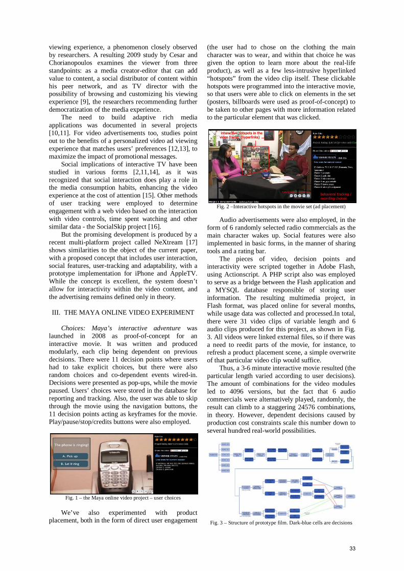
viewing experience, a phenomenon closely observed by researchers. A resulting 2009 study by Cesar and Chorianopoulos examines the viewer from three standpoints: as a media creator-editor that can add value to content, a social distributor of content within his peer network, and as TV director with the possibility of browsing and customizing his viewing experience [9], the researchers recommending further democratization of the media experience.
The need to build adaptive rich media applications was documented in several projects [10,11]. For video advertisements too, studies point out to the benefits of a personalized video ad viewing experience that matches users’ preferences [12,13], to maximize the impact of promotional messages.
Social implications of interactive TV have been studied in various forms [2,11,14], as it was recognized that social interaction does play a role in the media consumption habits, enhancing the video experience at the cost of attention [15]. Other methods of user tracking were employed to determine engagement with a web video based on the interaction with video controls, time spent watching and other similar data - the SocialSkip project [16].
But the promising development is produced by a recent multi-platform project called NeXtream [17] shows similarities to the object of the current paper, with a proposed concept that includes user interaction, social features, user-tracking and adaptability, with a prototype implementation for iPhone and AppleTV. While the concept is excellent, the system doesn’t allow for interactivity within the video content, and the advertising remains defined only in theory.
III. THE MAYA ONLINE VIDEO EXPERIMENT
Choices: Maya’s interactive adventure was
launched in 2008 as proof-of-concept for an interactive movie. It was written and produced modularly, each clip being dependent on previous decisions. There were 11 decision points where users had to take explicit choices, but there were also random choices and co-dependent events wired-in. Decisions were presented as pop-ups, while the movie paused. Users’ choices were stored in the database for reporting and tracking. Also, the user was able to skip through the movie using the navigation buttons, the 11 decision points acting as keyframes for the movie. Play/pause/stop/credits buttons were also employed.
Fig. 1 – the Maya online video project – user choices
We’ve also experimented with product
placement, both in the form of direct user engagement
(the user had to chose on the clothing the main character was to wear, and within that choice he was given the option to learn more about the real-life product), as well as a few less-intrusive hyperlinked “hotspots” from the video clip itself. These clickable hotspots were programmed into the interactive movie, so that users were able to click on elements in the set (posters, billboards were used as proof-of-concept) to be taken to other pages with more information related to the particular element that was clicked.
Fig. 2 –Interactive hotspots in the movie set (ad placement)
Audio advertisements were also employed, in the
form of 6 randomly selected radio commercials as the main character wakes up. Social features were also implemented in basic forms, in the manner of sharing tools and a rating bar.
The pieces of video, decision points and interactivity were scripted together in Adobe Flash, using Actionscript. A PHP script also was employed to serve as a bridge between the Flash application and a MYSQL database responsible of storing user information. The resulting multimedia project, in Flash format, was placed online for several months, while usage data was collected and processed.In total, there were 31 video clips of variable length and 6 audio clips produced for this project, as shown in Fig. 3. All videos were linked external files, so if there was a need to reedit parts of the movie, for instance, to refresh a product placement scene, a simple overwrite of that particular video clip would suffice.
Thus, a 3-6 minute interactive movie resulted (the particular length varied according to user decisions). The amount of combinations for the video modules led to 4096 versions, but the fact that 6 audio commercials were alternatively played, randomly, the result can climb to a staggering 24576 combinations, in theory. However, dependent decisions caused by production cost constraints scale this number down to several hundred real-world possibilities.
Fig. 3 – Structure of prototype film. Dark-blue cells are decisions
33
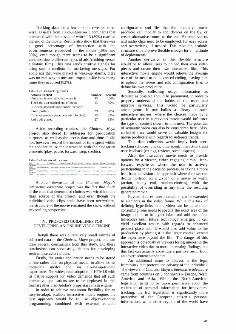
Tracking data for a few months revealed there were 33 users from 13 countries on 3 continents that interacted with the movie, of which 13 (39%) reached the end of the movie. Results also show that there was a good percentage of interaction with the advertisements embedded in the movie (39% and 88%), even though there seems to be a significant variation due to different types of ads (clothing versus a feature film). This data sends positive signals for using such a medium for marketing messages. For audio ads that were played as wake-up alarms, there was no real way to measure impact, aside how many times they occurred (82%).
Table 1 – User-tracking results
Actions tracked number percent Users that interacted with the movie 33 100% Times the user reached end of movie 13 39% Clicks on physical object inside the video frame (poster) 29 88% Clicks on product placement ads (clothing) 13 39% Radio ads played 27 82%
Aside recording choices, the Choices: Maya
project also stored IP addresses for geo-location purposes, as well as the access date and time. It did not, however, record the amount of time spent within the application, or the interaction with the navigation elements (play, pause, forward, stop, credits). Table 2 – Data stored for a user
Another downside of the Choices: Maya’s interactive adventure project was the fact that much of the code that determined choices was wired into the flash source of the project, and even though the individual video clips could have been overwritten, the structure of the movie remained the same, without any scaling perspective.
IV. PROPOSED GUIDELINES FOR DEVELOPING AN ONLINE VIDEO ENGINE
Though there was a relatively small sample of
collected data in the Choices: Maya project, one can draw several conclusions from this study, and these conclusions can serve as guidelines for developing such an interactive movie.
Firstly, the entire application needs to be stored online rather than on physical media, to allow for an open-data model and an always-up-to-date experience. The widespread adoption of HTML5 with its native support for video demands that all such interactive applications are to be deployed in this format rather than Adobe’s proprietary Flash engine.
In order to achieve maximum flexibility for an easy-to-adapt, scalable interactive movie engine, the best approach would be to use object-oriented programming, combined with external editable
configuration xml files that the interactive movie producer can modify to add choices on the fly, or create alternative routes to the end. External videos and audio clips need to be employed, for easy access and overwriting, if needed. This modular, scalable structure should prove flexible enough for a multitude of deployments.
Another derivative of this flexible structure would be to allow users to upload their own video pieces and create their own interactive film. This interactive movie engine would relieve the average user of the need to do advanced coding, leaving him to upload the videos and edit configuration files to define his own production.
Secondly, collecting usage information as detailed as possible should be paramount, in order to properly understand the habits of the users and improve services. This would be particularly advantageous if one builds a library of such interactive movies, where the choices made by a particular user in a previous movie would influence the type of content shown to him next. The potential of semantic video can also be considered here. Also, collected data would serve as valuable insight for movie producers with regards to audience trends.
This data collection would imply both user-tracking (choices, clicks, time spent, interaction), and user feedback (ratings, reviews, social aspects).
Also, the interactive movie needs to provide options for a viewer, either engaging himin lean-forward experience where the user is actively participating in the decision process, or taking a more lean-back television-like approach where the user can decide up-front on a „type” of a movie to watch (action, happy end, random-choices), with the possibility of overriding at any time the resulting generated movie.
Beyond choices, user interaction can be extended to elements in the video frame. While this task of defining hyperlinks in the video can be quite time-consuming (one needs to specify the exact area of the image that is to be hyperlinked and add the in/out timecode) until future technology emerges, it can yield excellent results with regards to enhanced product placement. It would also add value to the production by placing it in the larger context, extend the experience beyond the film. The danger of this approach is obviously of viewers losing interest in the interactive video due to more interesting findings, but this fact can actually constitute a positive result from an advertisement standpoint.
An additional issue to address is the legal framework that protects the privacy of the individual. The viewers of Choices: Maya’s interactive adventure came from countries on 3 continents – Europe, North America and Asia. While the North-American legislation tends to be more permissive about the collection of personal information for behavioural tracking, the EU legislation is significantly more protective of the European citizen’s personal information, while other regions of the world have
34

other restrictions [18,19]. Due to these geographical differences in legislation and the pervasiveness of the internet, it is recommended to implement an IP-filtering solution to block access from legally-problematic countries (which can also be coupled with geo-protection for copyrighted material). An even better alternative would be to build an upfront online form, requesting permission to track behavioral data from the user.
V. CONCLUSIONS AND FUTURE RESEARCH
This article presented an overview of current trends in interactive television. It then presented an experimental model called Choices: Maya’s interactive adventure, an interactive film that placed the user in charge of the narration, employing user-tracking to create a detailed profile of user choices and preferences and resorting to interactive ad-placement, both visual and audio. It then presented a set of guidelines for producing and deploying an interactive movie, focusing on generating a good degree of user participation and a pleasant experience, while at the same time exploring business opportunities for in-media advertising that would yield optimal results for ad companies.
An important direction for future research is evaluating how a lean-forward, decision-taking approach can be combined with a semantic approach, where the interactive system starts serving customized content that is adapted to the preferences of the user, once a certain acquaintance of user preferences and habits is obtained. This would lead to a more adaptable interactive system that is more sensitive to user location and context. A good balance between active input versus an adaptive automated experience based on media semantics should be researched in following studies.
Another area to explore would be improving the effectiveness of advertisements in such an interactive production. This would be of tremendous importance for the entertainment industry that relies heavily on the advertising model for generating revenues. Another opportunity would be to practically implement an engine for user-generated interactive videos, as well as finding more cost-effective ways to produce interactive movies.
ACKNOLEDGEMENT This work was partially supported by the strategic grant POSDRU 107/1.5/S/77265, inside POSDRU Romania 2007-2013 co-financed by the European Social Fund – Investing in People.
REFERENCES [1] ISuppli Research. (2010, Aug.) iSuppli Research.
[Online]. http://www.isuppli.com/Display-Materials-and-
Systems/MarketWatch/Pages/Internet-Enabled-TV-Trumps-3-D-TV-in-2010.aspx
[2] B. Lee and R. Lee, "How and why people watch TV: implications for the future of interactive television," Journal of Advertising Research, vol. 35, no. 6, pp. 9-18, Nov. 1995.
[3] J. Jensen, "Interactive Television - A Brief Media History," Changing Television Environments, vol. 5066, pp. 1-10, 2008.
[4] A. Collins, P. Neville, and K. Bielaczyc, "The Role of Different Media in Designing Learning," International Journal of Artificial Intelligence in Education, vol. 11, no. 11, pp. 144-162, 2000.
[5] M. Lytras, C. Lougos, P. Chozos, and A. Pouloudi, "Interactive Television and e-Learning Convergence: Examining the Potential of t-Learning, Lytras M. et al," Eltrun, 2002.
[6] J. Vendrig and M. Worring, "Interactive adaptive movie annotation," Multimedia, IEEE, 2003.
[7] M. Angelides and H. Agius, "An MPEG-7 scheme for semantic content modelling and filtering of digital video," Multimedia Systems, vol. 11, no. 4, pp. 320-339.
[8] M.-J. Montpetit, N. Klym, and T. Mirlacher, "The Future of IPTV Adding Social Networking and Mobility," in ConTEL 2009. 10th International Conference on Telecommunications, Zagreb, 2009, pp. 405-409.
[9] P. Cesar and K. Chorianopoulos, "The Evolution of TV Systems, Content and Users Toward Interactivity," Foundations and Trends in Human-Computer Interaction, vol. 2, no. 4, pp. 279-373, 2009.
[10] C. Wolf, "iWeaver: Towards an Interactive Web-Based Adaptive Learning Environment to Address Individual Learning Styles," European Journal of Open, Distance and E-Learning, 2002.
[11] D. Geerts and D. Grooff, "Supporting the Social Uses of Television: Sociability Heuristics for Social TV," in Proceedings of the 27th international conference on Human factors in computing systems, Boston, 2009, pp. 595-604.
[12] K. Chorianopoulos, G. Lekakos, and S. Diomidis, "Intelligent User Interfaces in the Living Room: Usability Design for Personalized Television Applications," in Proceedings of the 2003 International Conference on Intelligent User Interfaces, Miami, USA, 2003, pp. 230-232.
[13] S. Velusamy, L. Gopal, S. Bhatnagar, and S. Varadarajan, "An efficient ad recommendation system for TV programs ," Multimedia Systems, vol. 14, no. 2, pp. 73-87, Apr. 2008.
[14] L. Oehlberg, N. Ducheneaut, J. D. Thornton, R. J. Moore, and E. Nickell, "Social TV: Designing for Distributed, Sociable Television Viewing," in Proceedings of the EuroITV 2006 Conference,
35

Athens, 2006. [15] J. Weisz, et al., "Watching Together: Integrating
Text Chat with Video," in Proceedings of the SIGCHI conference on Human factors in computing system, San Jose, California, 2007, pp. 877-886.
[16] K. Chorianopoulos, I. Leftheriotis, and C. Gkonela, "SocialSkip: pragmatic understanding within web video," in Proceedings of the 9th international interactive conference on Interactive television, Lisbon, 2011, pp. 25-28.
[17] R. Martin, A. L. Santos, and M. Shafran, "neXtream: A Multi-Device, Social Approach to Video Content Consumption," in Proceedings of the 7th IEEE conference on Consumer communications and networking conference, Las Vegas, Nevada, USA, January 2010, pp. 779-783.
[18] G. Lasprogata, N. King, and S. Pillay, "Regulation of Electronic Employee Monitoring: Identifying Fundamental Principles of Employee Privacy through a Comparative Study of Data Privacy Legislation in the European Union, United States and Canada," Stanford Technology Law Review, vol. 4, 2004.
[19] G. Iachello and J. Hong, "End-user privacy in human-computer interaction," Foundations and Trends in Human-Computer Interaction, vol. 1, no. 1, pp. 1-137, Jan. 2007.
36

Buletinul Ştiinţific al Universităţii "Politehnica" din Timişoara
Seria ELECTRONICĂ şi TELECOMUNICAŢII
TRANSACTIONS on ELECTRONICS and COMMUNICATIONS
Tom 56(70), Fascicola 2, 2011
THE MPEG -7 QUERY OF THE E-LEARNING CONTENT
Andrei Marius Gabor1 Radu Vasiu2
1 Facultatea de Electronică şi Telecomunicaţii, Departamentul Comunicaţii Bd. V. Pârvan Nr. 2, 300223 Timişoara, e-mail [email protected] 2 Facultatea de Electronică şi Telecomunicaţii, Departamentul Comunicaţii Bd. V. Pârvan Nr. 2, 300223 Timişoara, e-mail [email protected]
Abstract– Based on nowadays progress, the quantity of multimedia data that is stored has increased progressively during the e-learning platforms. The value of multimedia information depends on the easiness of having access to it, filtering and managing. Therefore, there is the necessity of organizing and accessing the content efficiently, in order to help its user. The proposed architecture uses MP7QF framework specific to MPEG-7 standard to query multiple database in order to create, distribute and consume the returned digital information, in the e-learning context. Keywords: MPEG-7, multimedia database, MP7QF framework, e-learning
I. INTRODUCTION
Nowadays the e-learning field is given an increased attention due to the number and diversity of its users, beginning with the large companies and continuing with educational institution. The e-learning platforms have a unitary structure, have specific procedures for administration and documentation, the accomplishment of didactic activities ensure the interaction between its users or between groups of users, at the same time. The users, that can be an individual or a group of individual’s accesses the application based on a user name or on a access password. According to the groups which he/she belongs to, administrative procedures are activated, to create and populate the content, to inform or to consume it. The professors edit the courses for the students who attend specific classes. The students are given permission to have access and read the courses, by using the user name and the password. Moreover, the students can query different database, out of the system, to collect extra information.
The e-learning platforms are made of: LMS (Learning Management System), LCMS (Learning Content Management System) and web portal. [1]. LMS is a software application for administrating, documenting, checking and reporting the classes, the classrooms the events and the users. So, the main purpose of LMS is to offer the management of the classes and users. This thing can be accomplished through three user levels:
-the student, who uses the content and gains knowledge
-the professor, who elaborates the course and ensure the support for curses
-the administrator, who assigns the courses and the users LCMS (Learning Content Management System) is a technology related to the management system and aims at developing, managing and editing the content, which will be delivered through LMS. LCMS creates, storages and manages the digital content, as well as creates, imports, manages and searches for items of digital content, called learning object. These objects contain media files, assessment elements, text, graphics or any other object which forms the course content. Reusing of these objects in the context and the content of different courses is necessary many times. This is, in fact, the philosophy on which the portability of educational application is based, with the help of SCORM standard, implemented by IEEE Learning Technologies Committee [2]. The purpose of this paper is to give a system version which uses MP7QF framework, in order to provide a single access point to different information sources and to digital libraries (images, audio, video, text) in the e-learning context. I will introduce LO (Learning Object) features, and LOM standard, then I will
37
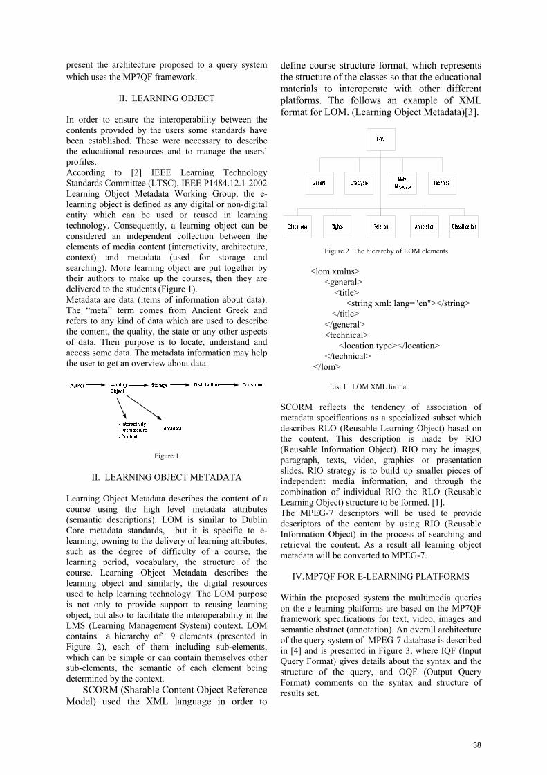
present the architecture proposed to a query system which uses the MP7QF framework.
II. LEARNING OBJECT
In order to ensure the interoperability between the contents provided by the users some standards have been established. These were necessary to describe the educational resources and to manage the users` profiles. According to [2] IEEE Learning Technology Standards Committee (LTSC), IEEE P1484.12.1-2002 Learning Object Metadata Working Group, the e-learning object is defined as any digital or non-digital entity which can be used or reused in learning technology. Consequently, a learning object can be considered an independent collection between the elements of media content (interactivity, architecture, context) and metadata (used for storage and searching). More learning object are put together by their authors to make up the courses, then they are delivered to the students (Figure 1). Metadata are data (items of information about data). The “meta” term comes from Ancient Greek and refers to any kind of data which are used to describe the content, the quality, the state or any other aspects of data. Their purpose is to locate, understand and access some data. The metadata information may help the user to get an overview about data.
Figure 1
II. LEARNING OBJECT METADATA
Learning Object Metadata describes the content of a course using the high level metadata attributes (semantic descriptions). LOM is similar to Dublin Core metadata standards, but it is specific to e-learning, owning to the delivery of learning attributes, such as the degree of difficulty of a course, the learning period, vocabulary, the structure of the course. Learning Object Metadata describes the learning object and similarly, the digital resources used to help learning technology. The LOM purpose is not only to provide support to reusing learning object, but also to facilitate the interoperability in the LMS (Learning Management System) context. LOM contains a hierarchy of 9 elements (presented in Figure 2), each of them including sub-elements, which can be simple or can contain themselves other sub-elements, the semantic of each element being determined by the context. SCORM (Sharable Content Object Reference Model) used the XML language in order to
define course structure format, which represents the structure of the classes so that the educational materials to interoperate with other different platforms. The follows an example of XML format for LOM. (Learning Object Metadata)[3].
Figure 2 The hierarchy of LOM elements <lom xmlns> <general> <title> <string xml: lang="en"></string> </title> </general> <technical> <location type></location> </technical> </lom> List 1 LOM XML format SCORM reflects the tendency of association of metadata specifications as a specialized subset which describes RLO (Reusable Learning Object) based on the content. This description is made by RIO (Reusable Information Object). RIO may be images, paragraph, texts, video, graphics or presentation slides. RIO strategy is to build up smaller pieces of independent media information, and through the combination of individual RIO the RLO (Reusable Learning Object) structure to be formed. [1]. The MPEG-7 descriptors will be used to provide descriptors of the content by using RIO (Reusable Information Object) in the process of searching and retrieval the content. As a result all learning object metadata will be converted to MPEG-7.
IV. MP7QF FOR E-LEARNING PLATFORMS Within the proposed system the multimedia queries on the e-learning platforms are based on the MP7QF framework specifications for text, video, images and semantic abstract (annotation). An overall architecture of the query system of MPEG-7 database is described in [4] and is presented in Figure 3, where IQF (Input Query Format) gives details about the syntax and the structure of the query, and OQF (Output Query Format) comments on the syntax and structure of results set.
38

-queries based by examples, in which the space and time relations will be used as well as the low level features and the semantic features. The user may select the needed image from the returning results, and if he/she is not satisfied, may reformulate the query.
-queries based on the MPEG-7 standard specification. Color and texture descriptors will be used for query as well as the description schemes.
-queries based on the preferences and the history of the user. Figure 3 The architecture format for MPEG-7 query
There is not a standard format to metadata query of MPEG-7, that is the reason why MPEG committee have decided framework (standardized ISO/IEC 15938-12) together with a set of requirements (N 8219). The objective of MP7QF framework is to provide an interface for MPEG-7 database in order to allow the users to retrieval the multimedia data. The student who attend the classes of a certain course, can make queries in the multiple database, and the result of the query to be based on his/her preferences and on the history use. The MP7QF framework must meet the following expectations in order to be used on the e-learning platforms:
<m7qf:Query > <m7qf:Input >
< m7qf:QueryCondition > < m7qf:QueryExpression > < m7qf:SingleSearch xsi:type =" m7qf:TextQueryType "retrieval =" contains "> < m7qf:FreeTextQuery > < m7qf:SearchTerm >Search object learning</ m7qf:SearchTerm > </ m7qf:FreeTextQuery > </ m7qf:SingleSearch > </ m7qf:QueryExpression > </ m7qf:QueryCondition >
- to allow the simultaneous searching within the multiple database, the way it is described in Figure 4, both on the e-learning platforms and on the external ones, meaning to allow a single query for the results received from the database.
</ m7qf:Input > </ m7qf:Query >
List 2 MP7QF query based on text descriptions
V. CONCLUSION - to accept the formats which are returned by the
query within the process of retrieval the multimedia data.
In this paper I propose an architecture for e-learning platforms. This architecture used the MP7QF framework specific to the MPEG-7 standard in order to query the multiple database. Additionally to the things mentioned above, in the future, I intend to study the way of conversing the MPEG-7 learning object metadata and their query, all these based on the semantics specifics to the e-learning field but also based on the preferences of the user.
ACKNOWLEDGMENT
“This work was partially supported by the strategic grant POSDRU 107/1.5/S/77265, inside POSDRU Romania 2007-2013 co-financed by the European Social Fund – Investing in People.”
Figure 4 The MP7QF query within the multiple database
REFERENCES The professors and the students can use the results of MP7QF query, results that can be RIO (Reusable Information Learning) or images, video, text either for creating another course or for the use of the content. The user must be able to choose, select and group the multimedia data according to the context and the e-learning content as a result of the query and of the returning of the result.
[1] http://www.fluidpower.ro/itfps/Etapa1ITFPS.pdf [2] IEEE Learning Technology Standardization Committee,
Draft Standard for Learning Object Metadata, 18 April2001. [3] Uche Ogbuji Thinking XML: Learning Objects Metadata
http://www.ibm.com/developerworks/xml/library/x-think21.html
[4] Mario Doller, Ingo Wolf, Matthias Gruhne, and HaraldKosch. Towards an MPEG-7 Query Language. In Proceedings of the International Conference on Signal-Image Technology and Internet Based Systems (IEEE/ACM SITIS 2006), pages 36–45, Hammamet, Tunesia, 2006.
The MP7QF framework must provide support/help for different queries [5]:
-description queries, which are based on text descriptions (described in List 2), but also using the description and the MPEG-7 description schemes.
[5] Kerstin Renner. Specification of an MPEG-7 Query Language, University of Pasau, Germany 2007.
39
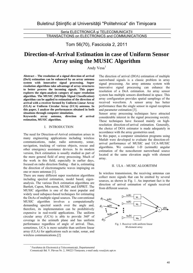
Buletinul Ştiinţific al Universităţii "Politehnica" din Timişoara
Seria ELECTRONICĂ şi TELECOMUNICAŢII TRANSACTIONS on ELECTRONICS and COMMUNICATIONS
Tom 56(70), Fascicola 2, 2011
Direction-of-Arrival Estimation in case of Uniform Sensor Array using the MUSIC Algorithm
Andy Vesa1
1
1 Facultatea de Electronică şi Telecomunicaţii, Departamentul Comunicaţii Bd. V. Pârvan Nr. 2, 300223 Timişoara, e-mail [email protected]
Abstract – The resolution of a signal direction of arrival (DoA) estimation can be enhanced by an array antenna system with innovative signal processing. Super resolution algorithms take advantage of array structures to better process the incoming signals. This paper explores the eigen-analysis category of super resolution algorithm. The MUSIC (MUltiple SIgnal Classification) algorithm can be applied to estimation of the direction of arrival with a receiver formed by Uniform Linear Array (ULA) or Uniform Circular Array (UCA) antenna. In this paper, I analyze the performances obtained in both situations through computer simulation. Keywords: array antenna, direction of arrival estimation, MUSIC algorithm.
I. INTRODUCTION
The need for Direction-of-Arrival estimation arises in many engineering applications including wireless communications, radar, radio astronomy, sonar, navigation, tracking of various objects, rescue and other emergency assistance devices. In its modern version, DoA estimation is usually studied as part of the more general field of array processing. Much of the work in this field, especially in earlier days, focused on radio direction finding – that is, estimating the direction of electromagnetic waves impinging on one or more antennas [1]. There are many different super resolution algorithms including spectral estimation, model based, eigen-analysis. The various DoA estimation algorithms are Bartlett, Capon, Min-norm, MUSIC and ESPRIT. The MUSIC algorithm is one of the most popular and widely used subspace-based techniques for estimating the DoAs of multiple signal sources. The conventional MUSIC algorithm involves a computationally demanding spectral search over the angle and, therefore, its implementation can be prohibitively expensive in real-world applications. The uniform circular array (UCA) is able to provide 360º of coverage in the azimuth plane and has uniform performance regardless of angle of arrival. Thus, sometimes, UCA is more suitable than uniform linear array (ULA) for applications such as radar, sonar, and wireless communications.[2]
The direction of arrival (DOA) estimation of multiple narrowband signals is a classic problem in array signal processing. An array antenna system with innovative signal processing can enhance the resolution of a DoA estimation. An array sensor system has multiple sensors distributed in space. This array configuration provides spatial samplings of the received waveform. A sensor array has better performance than the single sensor in signal reception and parameter estimation [3]. Sensor array processing techniques have attracted considerable interest in the signal processing society. These techniques have focused mainly on high-resolution direction-of-arrival estimation. Generally, the choice of DOA estimator is made adequately in accordance with the array geometries used. In this paper, a computer simulation programs using Matlab were developed to evaluate the direction-of-arrival performance of MUSIC and UCA-MUSIC algorithms. We consider 1-D (azimuth) angular estimation of the noncoherent narrowband source located at the same elevation angle with element array.
II. ULA – MUSIC ALGORITHM
In wireless transmission, the receiving antennas can collect more signals that can be emitted by several sources, as shown in Fig. 1. An important fact is the direction of arrival estimation of signals received from different sources.
φ
2φ
Dφ
s1(k)
s2(k)
sD(k)
x1(k)
x2
w 1 (k)
xM
w 2 y(k) +
(k) w M
Fig. 1. Receiver with uniform linear M-element array
40

It can be observed that the D signals arrive from D directions. They are received by an array of M elements with M potential weights. Many of the DoA algorithms rely on the array correlation matrix. In order to simplify the notation let us define the M x M array correlation matrix Rxx as [4]:
( )( )
.
H H Hxx
H H H
Hss nn
R E x x E As n s A n
AE s s A E n n
AR A R
⎡ ⎤⎡ ⎤= ⋅ = + +⎢ ⎥⎣ ⎦ ⎣ ⎦⎡ ⎤ ⎡ ⎤= ⋅ + ⋅⎣ ⎦ ⎣ ⎦
= +
H
I
. (1)
where RSS represents the source correlation matrix (D x D elements), 2
nn nR σ= represents the noise correlation matrix (M x M elements), and I represents the identity matrix (N x N elements). Given M-array elements with D-narrowband signal sources and uncorrelated noise, we can make some assumptions about the properties of the correlation matrix: is an MxM Hermitian matrix. The array correlation matrix has M eigenvalues ( 1 2, , , Mλ λ λK ) along with associated eigenvectors 1 2 ME e e e⎡ ⎤= ⎣ ⎦L If the eigenvalues are
sorted from smallest to largest, we can divide the matrix E into two subspaces: N SE E E⎡= ⎣ ⎤⎦
. The first
subspace NE is called the noise subspace and is composed of M – D eigenvectors associated with the noise, and the second subspace SE is called the signal subspace and is composed of D eigenvectors associated with the arriving signals. The noise subspace is an M x (M – D) matrix, and the signal subspace is an (M x D) matrix. The MUSIC algorithm is based on the assumption that the noise subspace eigenvectors are orthogonal to the array steering vectors, ( )a φ , at the angles of arrival
1 2, , , Dφ φ φK . Because of this orthogonality condition, one can show that the Euclidian distance
2 ( ) ( ) 0H HN Nd a E E aφ φ= = for each and every arrival
angle 1 2, , , Dφ φ φK . Placing this distance expression in the denominator creates sharp peaks at the angles of arrival. The MUSIC pseudospectrum is: ( )
( ) ( )1 .MUSIC HHN N
Pa E E a
θφ φ
= . (2)
III. UCA – MUSIC ALGORITHM
Consider a UCA consisting of M identical elements uniformly distributed over the circumference of a circle of radius r. Assume that D narrowband sources, centered on wavelength λ, impinge on the array from directions iφ (i=1, … ,D), respectively, where
[ )0, 2iφ π∈ is the azimuth angle measured from the x-axis counter-clockwise. Figure 2 depicts a receiver formed by an uniform circular array with incident planewaves from various directions.
The Mx1 vector received by the array is expressed by[5]: ( )( ) ( ) ( )y k C A s k n kφ= + . (3) where ( ) 1[ ( ) ( )]DA a aφ φ φ= K is the MxD matrix of the steering vectors, s(k) = [s1(k), … , sD(k)]T is the Dx1 signal vector, n(k) = [ n1(k), … , nM(k)]T is the
1 noise vector. The signal vector s(k) and the vector n(k) of the additive and spatially white noise are assumed to be statistically independent and zero-mean. The MxM matrix
Mx
C is the mutual coupling matrix. Due to the circular symmetry, a model for the mutual coupling matrix of UCAs [6] can be a complex symmetric circulant matrix. The steering vector with mutual coupling can be modeled as: ( ) ( )a C aφ φ=% . (4) The covariance matrix R of the received data is constructed and an eigendecomposition of R results in a signal and noise subspace:
( ) ( )H
H Hs s s n n n
R E x k x k
E E E E
= =
= Λ + Λ. (5)
where sE and nE denote the signal and noise subspace eigenvectors and the diagonal matrices sΛ and nΛ contain the signal subspace and noise subspace eigenvalues. The MUSIC algorithm estimates the DOAs from the D deepest nulls of the UCA - MUSIC function: ( ) ( ) ( )H H
UCA MUSIC n nf a E E aφ φ φ− = % % . (6)
IV. SIMULATION RESULTS In this section, computer simulations are provided to substantiate the performance analysis. In all cases, the impinging angles of the sources are relative to the broadside of a uniform array. It is considered that the source is placed on the direction 20φ = + o
r
M
x
y
z
1
2
1φφ
Dφ
S1
S2(k)
SD(k)
M
Fig. 2. Receiver with unifor rcular M-element array
(k)
2
m ci
41
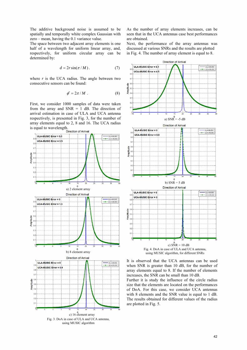
The additive background noise is assumed to be spatially and temporally white complex Gaussian with zero – mean, having the 0.1 variance value. The space between two adjacent array elements is one half of a wavelength for uniform linear array, and, respectively, for uniform circular array can be determined by: 2 sin( / )d r Mπ= . (7) where r is the UCA radius. The angle between two consecutive sensors can be found: 2 / Mφ π′ = . (8) First, we consider 1000 samples of data were taken from the array and SNR = 1 dB. The direction of arrival estimation in case of ULA and UCA antenna respectively, is presented in Fig. 3, for the number of array elements equal to 2, 8 and 16. The UCA radius is equal to wavelength.
As the number of array elements increases, can be seen that in the UCA antennas case best performances are obtained. Next, the performance of the array antennas was discussed at various SNRs and the results are plotted in Fig. 4. The number of array element is equal to 8.
It is observed that the UCA antennas can be used when SNR is greater than 10 dB, for the number of array elements equal to 8. If the number of elements increases, the SNR can be small than 10 dB. Further it is study the influence of the circle radius size that the elements are located on the performances of DoA. For this case, we consider UCA antennas with 8 elements and the SNR value is equal to 1 dB. The results obtained for different values of the radius are plotted in Fig. 5.
a) 2 element array
b) 8 element array
c) 16 element array Fig. 3. DoA in case of ULA and UCA antenna,
using MUSIC algorithm
a) SNR = -5 dB
b) SNR = 5 dB
c) SNR = 10 dB Fig. 4. DoA in case of ULA and UCA antenna,
using MUSIC algorithm, for different SNRs
42

[5] Y. Morikawa, N. Kikuma, K. Sakakibara, H. Hirayama, “DOA Estimation with Uniform Circular Array Using Gauss-Newton Method Based on MUSIC and MODE Algorithms”, Proceedings of ISAP, Seoul, Korea, 2005, pp. 317
[6] B. Friedlander, A. J. Weiss, “Direction finding in the presence of mutual coupling", IEEE Trans. Antennas Propag., Vol. 39, 1991, pp. 273
a) Radius equal to half wavelength
b) Radius equal to 2λ Fig. 5. DoA in case of UCA antenna,
using MUSIC algorithm, for different values of radius
Can be seen that, for a greater radius, are obtained good performances.
V. CONCLUSIONS In this paper, I give extensive computer simulation results to demonstrate the performances of the UCA antennas obtained in case of DoA estimation. The estimation of direction of arrival for one source of signal is implemented by using the MUSIC algorithm. The performances of DoA estimation obtained in case of ULA antenna are better than in case of UCA antenna. It is observed that the UCA antenna is not so powerful, but in some cases the results obtained with this system are acceptable.
REFERENCES [1] E. Tuncer and B. Friedlander, Classical and Modern Direction-of-Arrival Estimation, Ed. Elsevier,USA, 2009. [2] C. P. Mathews, M. D. Zoltowski, Signal Subspace Techniques for Source Localization with Circular Sensor Arrays, School of Electrical Engineering, Purdue University, West Lafayette, ECE-Technical Reports, 1994. [3] H. Hwang et al., “Direction of Arrival Estimation using a Root-MUSIC Algorithm,” Proceedings of the International MultiConference of Engineers and Computer Scientists, vol. II, Hong Kong, March 2008 [4] F. Gross, Smart Antennas for Wireless Communications – with MATLAB, Ed. New York: McGraw-Hill, 2005
43

Buletinul Ştiinţific al Universităţii "Politehnica" din Timişoara
Seria ELECTRONICĂ şi TELECOMUNICAŢII TRANSACTIONS on ELECTRONICS and COMMUNICATIONS
Tom 56(70), Fascicola 2, 2011
Instructions for authors at the Scientific Bulletin of the Politehnica University of Timisoara - Transactions on
Electronics and Communications
First Author1 Second Author2
1 Faculty of Electronics and Telecommunications, Communications Dept. Bd. V. Parvan 2, 300223 Timisoara, Romania, e-mail [email protected] 2 Faculty of Electronics and Telecommunications, Communications Dept. Bd. V. Parvan 2, 300223 Timisoara, Romania, e-mail [email protected]
Abstract – These instructions present a model for editing the papers accepted for publication in the Scientific Bulletin of “Politehnica” University of Timisoara, Transactions on Electronics and Communications. The abstract should contain the description of the problem, methods, solutions and results in a maximum of 12 lines. No references are allowed here. Keywords: editing, Bulletin, author
I. INTRODUCTION
The page format is A4. The articles must be of 6 pages or less, tables and figures included.
II. GUIDELINES Fig. 1. Amplitudes in the standing wave
The paper should be sent in this standard form. Use a good quality printer, and print on a single face of the sheet. Use a double column format with 0.5 cm in between columns, on an A4, portrait oriented, standard size. The top and bottom margins should be of 2.28 cm, and the left and right margins of 2.54 cm. Microsoft Word™ for Windows is recommended as a text editor. Choose Times New Roman fonts, and single spaced lines. Font sizes should be: 18 pt bold for the paper title, 12 pt for the author(s), 9 pt bold for the abstract and keywords, 10 pt capitals for the section titles, 10 pt italic for the subsection titles; distance between section numbers and titles should be of 0.25 cm; use 10 pt for the normal text, 8 pt for affiliation, footnotes, figure captions, and references.
III. FIGURES AND TABLES Figures should be centered, and tables should be left aligned, and should be placed after the first reference in the text. Use abbreviations such as “Fig.1.” even at the beginning of the sentence. Leave an empty line before and after equations. Equation numbering should be simple: (1), (2), (3) … and right aligned:
. (16) ∫− −=a
adtytx ττ )()(
IV. ABOUT REFERENCES References should be numbered in a simple form [1], [2], [3]…, and quoted accordingly [1]. References are not allowed in footnotes. It is recommended to mention all authors; “et al.” should be used only for more than 6 authors. Table 1
Parameter Value Unit I 2.4 A U 10.0 V
V. REMARKS A. Abbreviations and acronyms
44

Abbreviations and acronyms should be explained when they appear for the first time in the text. Abbreviations such as IEEE, IEE, SI, MKS, CGS, ac, dc and rms need no further explanation. It is
commended not to use abbreviations in section or bsection titles.
x SI and CGS. Preliminary, experimental sults are not accepted. Roman section numbering is
optional.
icrowave Engineering, Second raw-Hill, Inc., 1992.
[3] http://www.tc.etc.upt.ro/bulletin
resu
B. Further recommendations The International System of units is recommended. Do not mire
REFERENCES
[1] A. Ignea, “Preparation of papers for the International Symposium Etc. ’98”, Buletinul Universităţii “Politehnica”, Seria Electrotehnica, Electronica si Telecomunicatii, Tom 43 (57), 1998, Fascicola 1, 1998, pp. 81.
Foundations for M[2] R. E. Collin, Edition, McG
45