
Edge Detection Selim Aksoy Department of Computer Engineering Bilkent University...
91
-
Upload
kassandra-carbine -
Category
Documents
-
view
219 -
download
0
Transcript of Edge Detection Selim Aksoy Department of Computer Engineering Bilkent University...
CS 484, Spring 2010 ©2010, Selim Aksoy 2
Edge detection
Edge detection is the process of finding meaningful transitions in an image.
The points where sharp changes in the brightness occur typically form the border between different objects or scene parts.
These points can be detected by computing intensity differences in local image regions.
Initial stages of mammalian vision systems also involve detection of edges and local features.

CS 484, Spring 2010 ©2010, Selim Aksoy 3
Edge detection Sharp changes in the image brightness
occur at: Object boundaries
A light object may lie on a dark background or a dark object may lie on a light background.
Reflectance changes May have quite different characteristics - zebras have
stripes, and leopards have spots. Cast shadows Sharp changes in surface orientation
Further processing of edges into lines, curves and circular arcs result in useful features for matching and recognition.
CS 484, Spring 2010 ©2010, Selim Aksoy 4
Edge detection
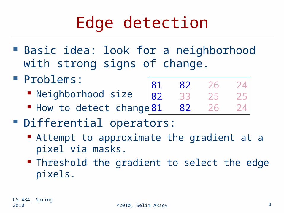
Basic idea: look for a neighborhood with strong signs of change.
Problems: Neighborhood size How to detect change
Differential operators: Attempt to approximate the gradient at a pixel
via masks. Threshold the gradient to select the edge pixels.
81 82 26 2482 33 25 2581 82 26 24
CS 484, Spring 2010 ©2010, Selim Aksoy 5
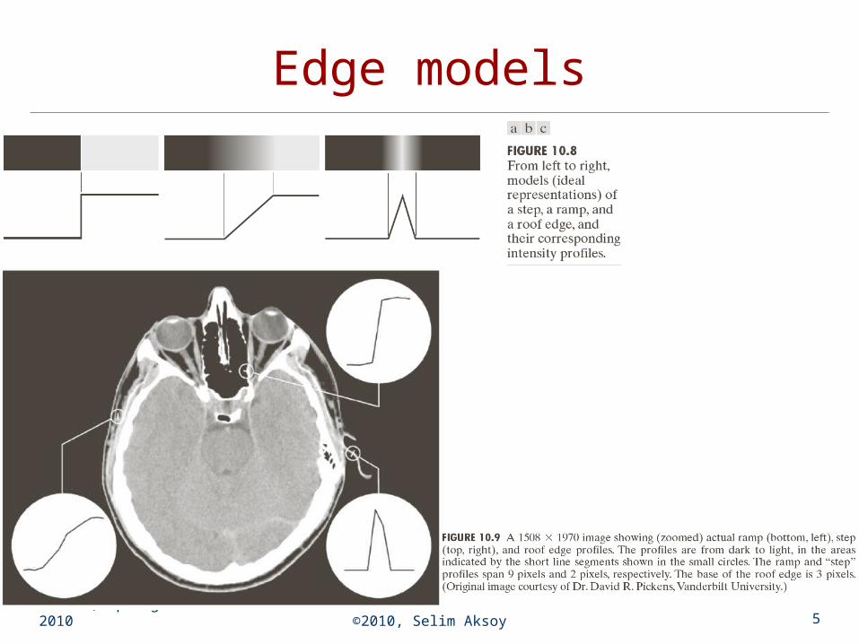
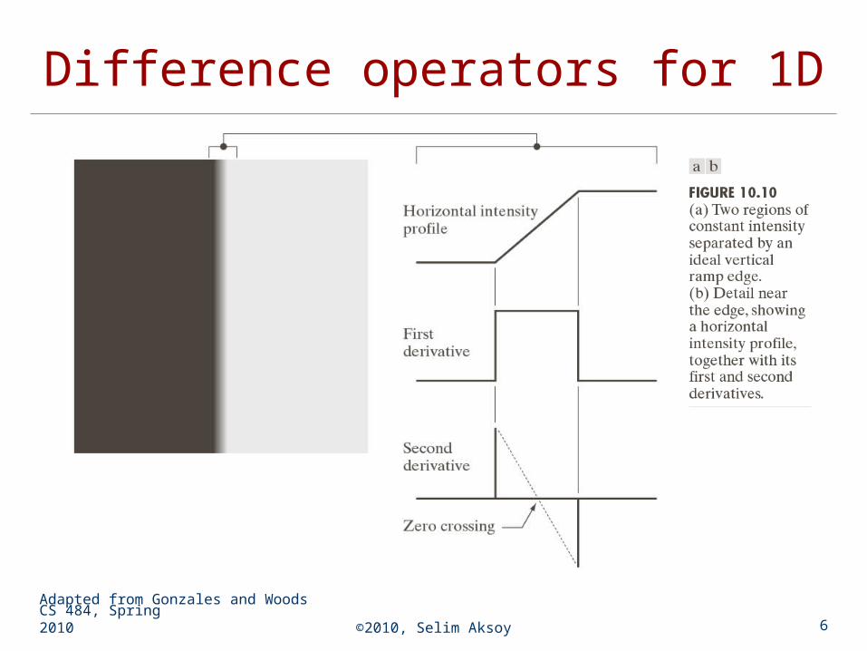
Edge models
CS 484, Spring 2010 ©2010, Selim Aksoy 6
Difference operators for 1D
Adapted from Gonzales and Woods

CS 484, Spring 2010 ©2010, Selim Aksoy 7
Difference operators for 1D
Adapted from Gonzales and Woods

CS 484, Spring 2010 ©2010, Selim Aksoy 8
Edge detection
Three fundamental steps in edge detection:1. Image smoothing: to reduce the effects
of noise.2. Detection of edge points: to find all
image points that are potential candidates to become edge points.
3. Edge localization: to select from the candidate edge points only the points that are true members of an edge.

CS 484, Spring 2010 ©2010, Selim Aksoy 9
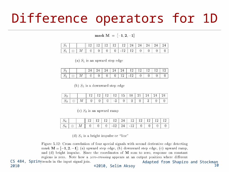
Difference operators for 1D
Adapted from Shapiro and Stockman
CS 484, Spring 2010 ©2010, Selim Aksoy 10
Difference operators for 1D
Adapted from Shapiro and Stockman

CS 484, Spring 2010 ©2010, Selim Aksoy 11
Observations
Properties of derivative masks: Coordinates of derivative masks have opposite
signs in order to obtain a high response in signal regions of high contrast.
The sum of coordinates of derivative masks is zero so that a zero response is obtained on constant regions.
First derivative masks produce high absolute values at points of high contrast.
Second derivative masks produce zero-crossings at points of high contrast.

CS 484, Spring 2010 ©2010, Selim Aksoy 12
Smoothing operators for 1D

CS 484, Spring 2010 ©2010, Selim Aksoy 13
Observations
Properties of smoothing masks: Coordinates of smoothing masks are positive
and sum to one so that output on constant regions is the same as the input.
The amount of smoothing and noise reduction is proportional to the mask size.
Step edges are blurred in proportion to the mask size.

CS 484, Spring 2010 ©2010, Selim Aksoy 14
Difference operators for 2D

CS 484, Spring 2010 ©2010, Selim Aksoy 15
Difference operators for 2D

CS 484, Spring 2010 ©2010, Selim Aksoy 16
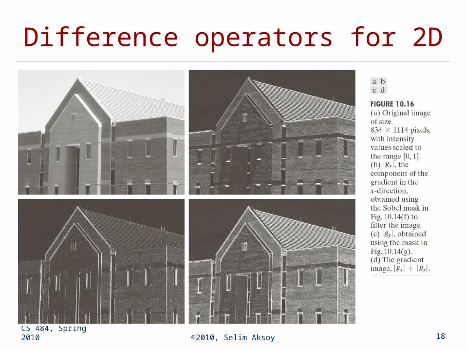
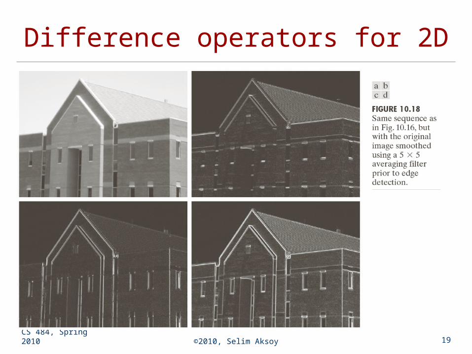
Difference operators for 2D
Adapted from Gonzales and Woods

CS 484, Spring 2010 ©2010, Selim Aksoy 17
Difference operators for 2D
original image gradient thresholded magnitude gradient magnitude
Adapted from Linda Shapiro, U of Washington
CS 484, Spring 2010 ©2010, Selim Aksoy 18
Difference operators for 2D
CS 484, Spring 2010 ©2010, Selim Aksoy 19
Difference operators for 2D

CS 484, Spring 2010 ©2010, Selim Aksoy 20
Difference operators for 2D

CS 484, Spring 2010 ©2010, Selim Aksoy 21
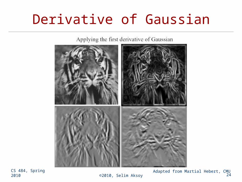
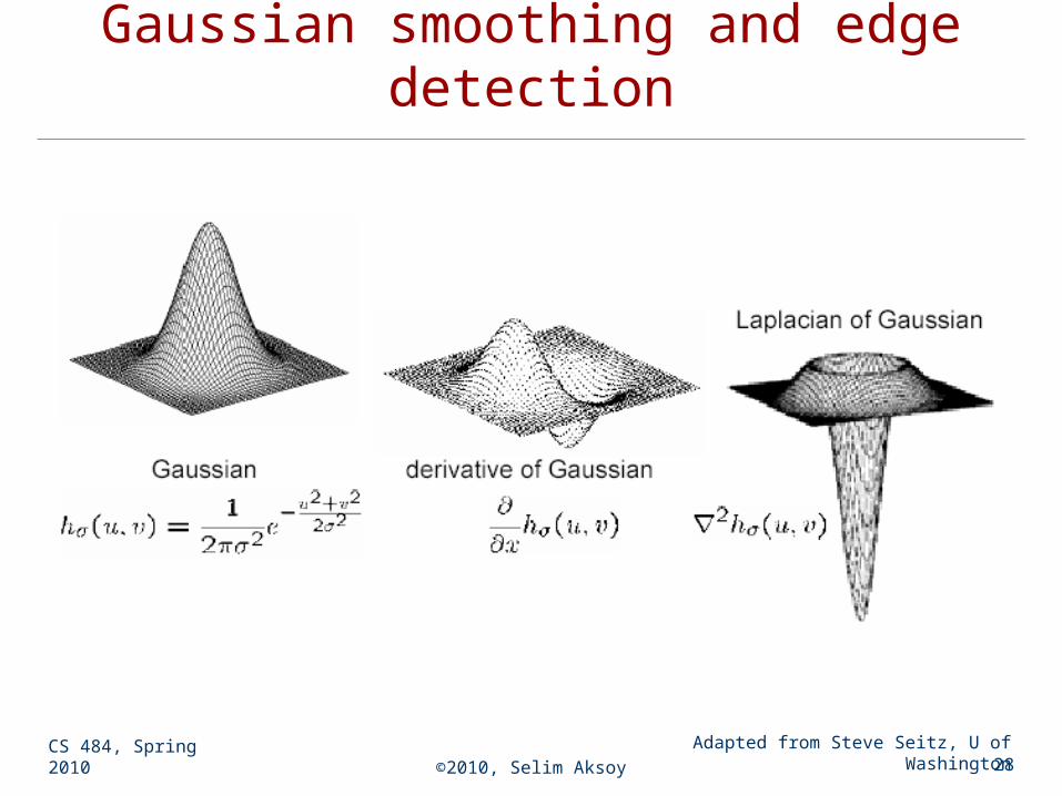
Gaussian smoothing and edge detection
We can smooth the image using a Gaussian filter and then compute the derivative.
Two convolutions: one to smooth, then another one to differentiate? Actually, no - we can use a derivative of Gaussian filter because differentiation is convolution and convolution is associative.

CS 484, Spring 2010 ©2010, Selim Aksoy 22
Derivative of Gaussian
Adapted from Michael Black, Brown University

CS 484, Spring 2010 ©2010, Selim Aksoy 23
Derivative of Gaussian
Adapted from Michael Black, Brown University
CS 484, Spring 2010 ©2010, Selim Aksoy 24
Derivative of Gaussian
Adapted from Martial Hebert, CMU
CS 484, Spring 2010 ©2010, Selim Aksoy 25
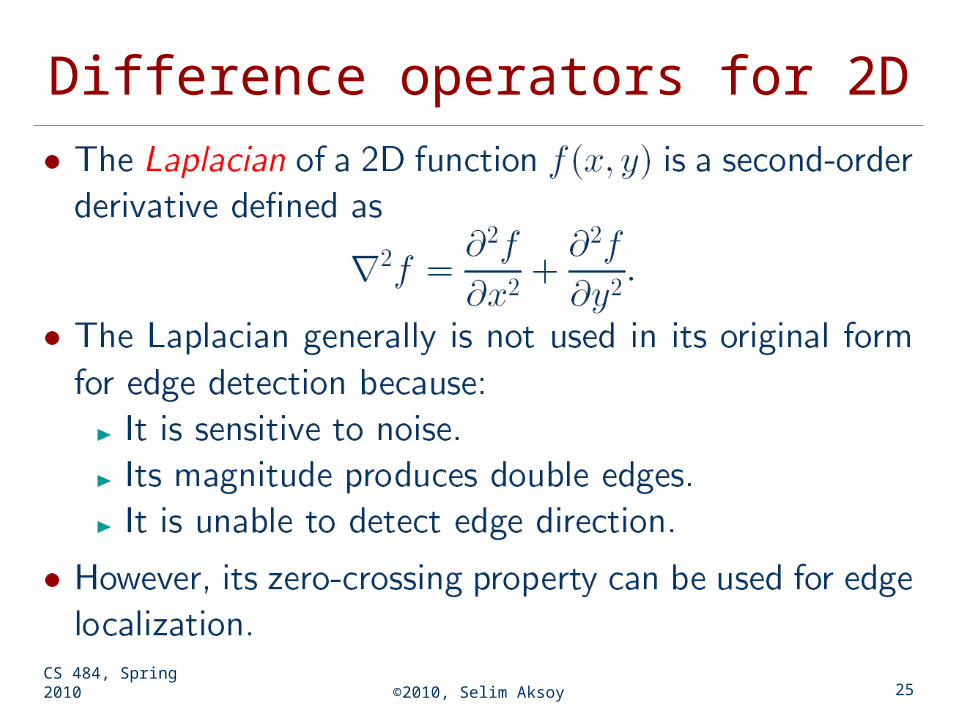
Difference operators for 2D

CS 484, Spring 2010 ©2010, Selim Aksoy 26
Gaussian smoothing and edge detection

CS 484, Spring 2010 ©2010, Selim Aksoy 27
Gaussian smoothing and edge detection
Adapted from Shapiro and Stockman
CS 484, Spring 2010 ©2010, Selim Aksoy 28
Gaussian smoothing and edge detection
Adapted from Steve Seitz, U of Washington

CS 484, Spring 2010 ©2010, Selim Aksoy 29
Laplacian of Gaussian
Adapted from Gonzales and Woods

CS 484, Spring 2010 ©2010, Selim Aksoy 30
Laplacian of Gaussian
Adapted from Shapiro and Stockman
CS 484, Spring 2010 ©2010, Selim Aksoy 31
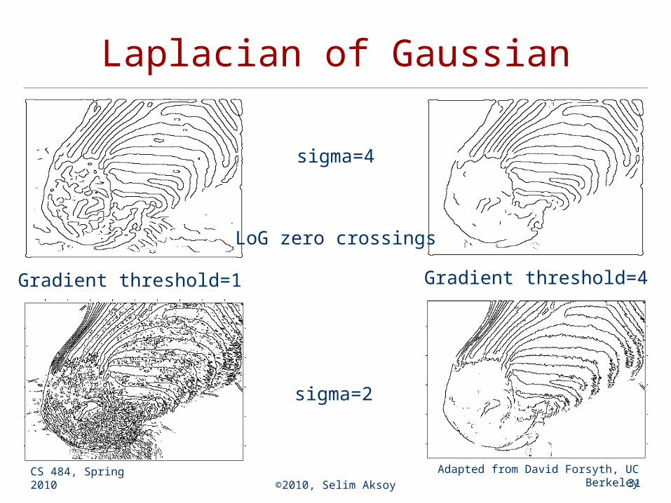
Laplacian of Gaussian
sigma=2
sigma=4
Gradient threshold=1 Gradient threshold=4
LoG zero crossings
Adapted from David Forsyth, UC Berkeley
CS 484, Spring 2010 ©2010, Selim Aksoy 32
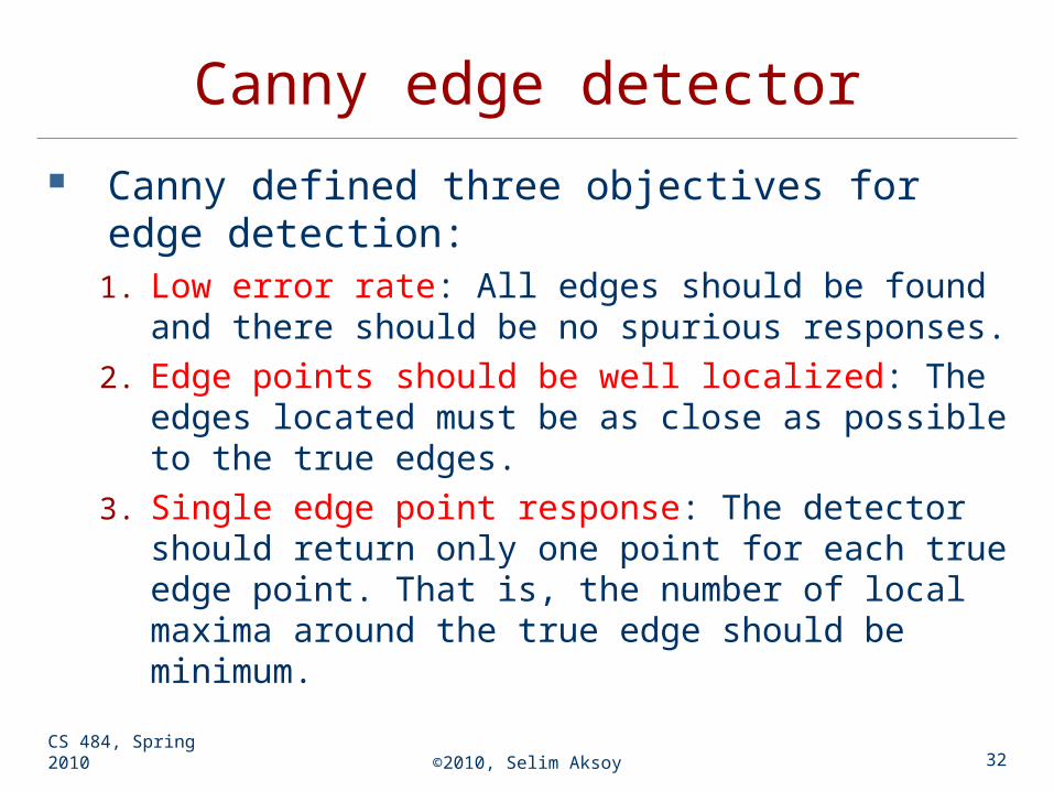
Canny edge detector
Canny defined three objectives for edge detection:1. Low error rate: All edges should be found and
there should be no spurious responses.2. Edge points should be well localized: The edges
located must be as close as possible to the true edges.
3. Single edge point response: The detector should return only one point for each true edge point. That is, the number of local maxima around the true edge should be minimum.
CS 484, Spring 2010 ©2010, Selim Aksoy 33
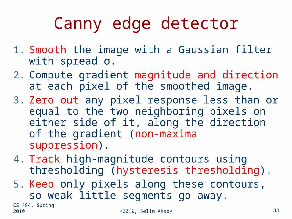
Canny edge detector
1. Smooth the image with a Gaussian filter with spread σ.
2. Compute gradient magnitude and direction at each pixel of the smoothed image.
3. Zero out any pixel response less than or equal to the two neighboring pixels on either side of it, along the direction of the gradient (non-maxima suppression).
4. Track high-magnitude contours using thresholding (hysteresis thresholding).
5. Keep only pixels along these contours, so weak little segments go away.

CS 484, Spring 2010 ©2010, Selim Aksoy 34
Canny edge detector Non-maxima
suppression: Gradient direction is
used to thin edges by suppressing any pixel response that is not higher than the two neighboring pixels on either side of it along the direction of the gradient.
This operation can be used with any edge operator when thin boundaries are wanted.
Note: Brighter squares illustrate stronger edge response.
Adapted from Martial Hebert, CMU

CS 484, Spring 2010 ©2010, Selim Aksoy 35
Canny edge detector
Hysteresis thresholding: Once the gradient magnitudes are thinned, high
magnitude contours are tracked. In the final aggregation phase, continuous
contour segments are sequentially followed. Contour following is initiated only on edge pixels
where the gradient magnitude meets a high threshold.
However, once started, a contour may be followed through pixels whose gradient magnitude meet a lower threshold (usually about half of the higher starting threshold).

CS 484, Spring 2010 ©2010, Selim Aksoy 36
Canny edge detector
Adapted from Martial Hebert, CMU

CS 484, Spring 2010 ©2010, Selim Aksoy 37
Canny edge detector
Adapted from Martial Hebert, CMU

CS 484, Spring 2010 ©2010, Selim Aksoy 38
Canny edge detector
Adapted from Martial Hebert, CMU

CS 484, Spring 2010 ©2010, Selim Aksoy 39
Canny edge detector
Adapted from Martial Hebert, CMU
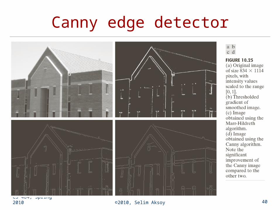
CS 484, Spring 2010 ©2010, Selim Aksoy 40
Canny edge detector
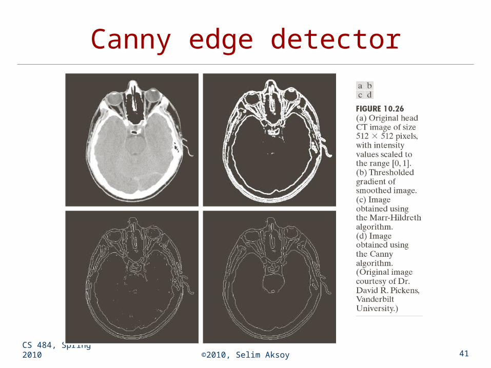
CS 484, Spring 2010 ©2010, Selim Aksoy 41
Canny edge detector

CS 484, Spring 2010 ©2010, Selim Aksoy 42
Canny edge detector
The Canny operator gives single-pixel-wide images with good continuation between adjacent pixels.
It is the most widely used edge operator today; no one has done better since it came out in the late 80s. Many implementations are available.
It is very sensitive to its parameters, which need to be adjusted for different application domains.

CS 484, Spring 2010 ©2010, Selim Aksoy 43
Edge linking
Hough transform Finding line segments Finding circles
Model fitting Fitting line segments Fitting ellipses
Edge tracking

CS 484, Spring 2010 ©2010, Selim Aksoy 44
Hough transform The Hough transform is a method for detecting
lines or curves specified by a parametric function.
If the parameters are p1, p2, … pn, then the Hough procedure uses an n-dimensional accumulator array in which it accumulates votes for the correct parameters of the lines or curves found on the image.
y = mx + b
image m
b
accumulator
Adapted from Linda Shapiro, U of Washington

CS 484, Spring 2010 ©2010, Selim Aksoy 45
Hough transform: line segments
Adapted from Steve Seitz, U of Washington

CS 484, Spring 2010 ©2010, Selim Aksoy 46
Hough transform: line segments
Adapted from Steve Seitz, U of Washington

CS 484, Spring 2010 ©2010, Selim Aksoy 47
Hough transform: line segments
Adapted from Gonzales and Woods

CS 484, Spring 2010 ©2010, Selim Aksoy 48
Hough transform: line segments
y = mx + b is not suitable (why?) The equation generally used is:
d = r sin(θ) + c cos(θ).
d
r
c
d is the distance from the line to origin.
θ is the angle the perpendicular makes with the column axis.
Adapted from Linda Shapiro, U of Washington
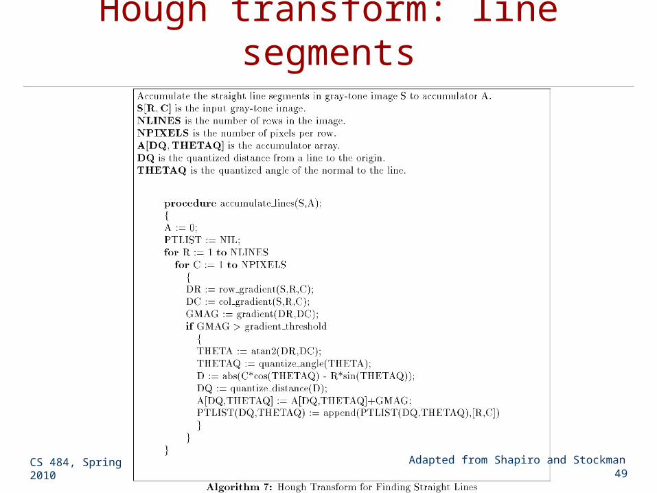
CS 484, Spring 2010 ©2010, Selim Aksoy 49
Hough transform: line segments
Adapted from Shapiro and Stockman

CS 484, Spring 2010 ©2010, Selim Aksoy 50
Hough transform: line segments
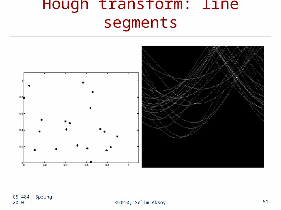
CS 484, Spring 2010 ©2010, Selim Aksoy 51
Hough transform: line segments

CS 484, Spring 2010 ©2010, Selim Aksoy 52
Hough transform: line segments
Extracting the line segments from the accumulators:
1. Pick the bin of A with highest value V2. While V > value_threshold {
1. order the corresponding pointlist from PTLIST2. merge in high gradient neighbors within 10
degrees3. create line segment from final point list4. zero out that bin of A5. pick the bin of A with highest value V
}Adapted from Linda Shapiro, U of
Washington

CS 484, Spring 2010 ©2010, Selim Aksoy 53
Hough transform: line segments
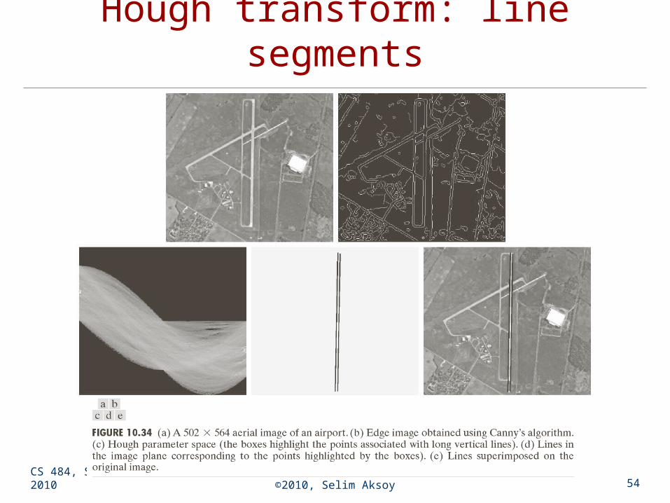
CS 484, Spring 2010 ©2010, Selim Aksoy 54
Hough transform: line segments

CS 484, Spring 2010 ©2010, Selim Aksoy 55
Hough transform: circles
Main idea: The gradient vector at an edge pixel points the center of the circle.
Circle equations: r = r0 + d sin(θ) r0, c0, d are parameters c = c0 + d cos(θ)
*(r,c)d
Adapted from Linda Shapiro, U of Washington

CS 484, Spring 2010 ©2010, Selim Aksoy 56
Hough transform: circles
Adapted from Shapiro and Stockman
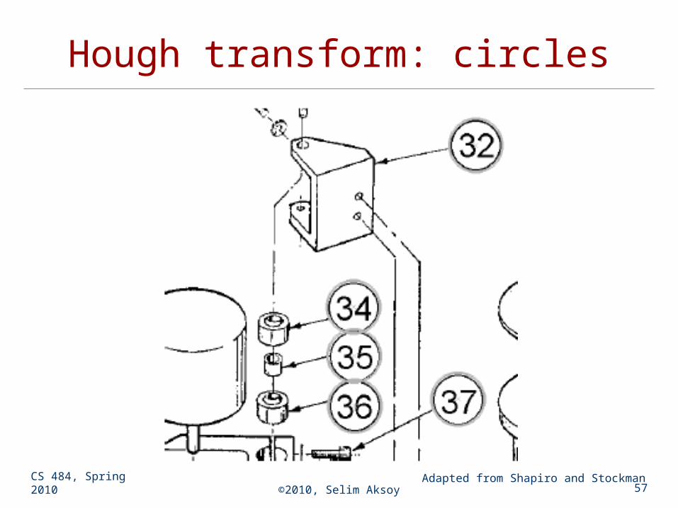
CS 484, Spring 2010 ©2010, Selim Aksoy 57
Hough transform: circles
Adapted from Shapiro and Stockman

CS 484, Spring 2010 ©2010, Selim Aksoy 58
Hough transform: circles
Adapted from Shapiro and Stockman

CS 484, Spring 2010 ©2010, Selim Aksoy 59
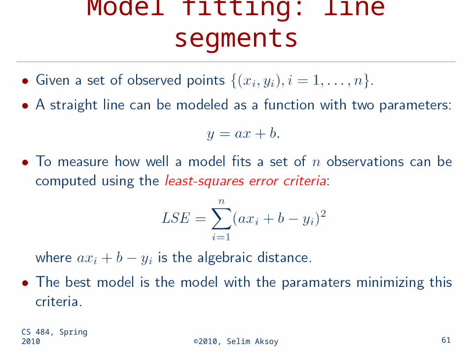
Model fitting Mathematical models that fit data not only reveal
important structure in the data, but also can provide efficient representations for further analysis.
Mathematical models exist for lines, circles, cylinders, and many other shapes.
We can use the method of least squares for determining the parameters of the best mathematical model fitting the observed data.
CS 484, Spring 2010 ©2010, Selim Aksoy 60
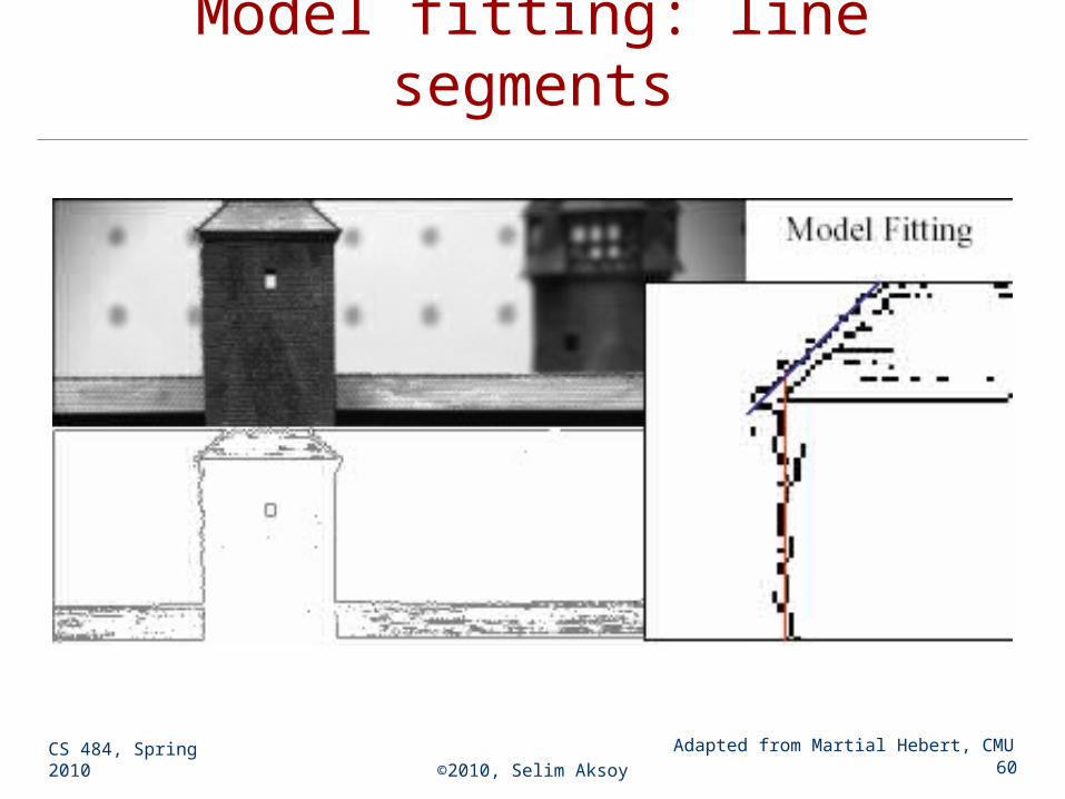
Model fitting: line segments
Adapted from Martial Hebert, CMU
CS 484, Spring 2010 ©2010, Selim Aksoy 61
Model fitting: line segments
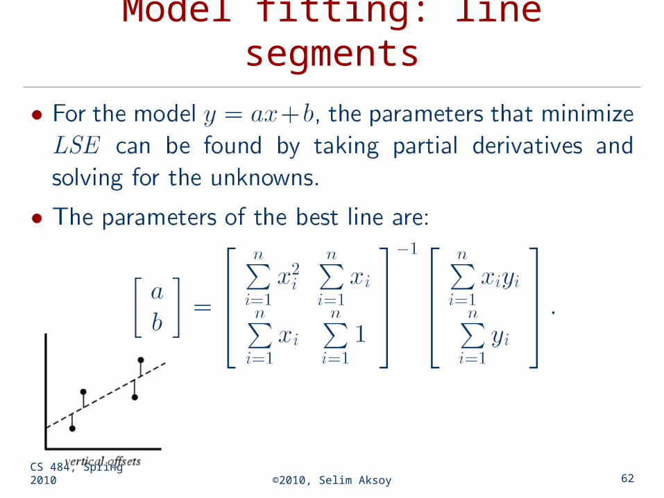
CS 484, Spring 2010 ©2010, Selim Aksoy 62
Model fitting: line segments

CS 484, Spring 2010 ©2010, Selim Aksoy 63
Model fitting: line segments

CS 484, Spring 2010 ©2010, Selim Aksoy 64
Model fitting: line segments
Problems in fitting: Outliers Error definition (algebraic vs. geometric
distance) Statistical interpretation of the error (hypothesis
testing) Nonlinear optimization High dimensionality (of the data and/or the
number of model parameters) Additional fit constraints
CS 484, Spring 2010 ©2010, Selim Aksoy 65
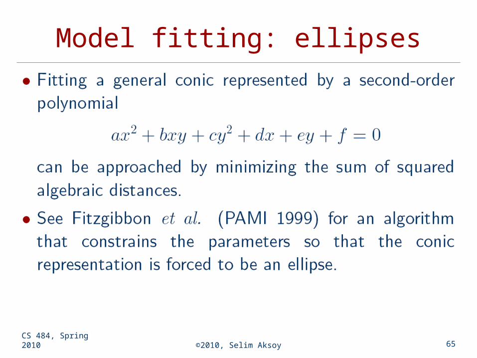
Model fitting: ellipses

CS 484, Spring 2010 ©2010, Selim Aksoy 66
Model fitting: ellipses
Adapted from Andrew Fitzgibbon, PAMI 1999

CS 484, Spring 2010 ©2010, Selim Aksoy 67
Model fitting: ellipses
Adapted from Andrew Fitzgibbon, PAMI 1999

CS 484, Spring 2010 ©2010, Selim Aksoy 68
Model fitting: incremental line fitting
Adapted from David Forsyth, UC Berkeley

CS 484, Spring 2010 ©2010, Selim Aksoy 69
Model fitting: incremental line fitting
Adapted from Trevor Darrell, MIT

CS 484, Spring 2010 ©2010, Selim Aksoy 70
Model fitting: incremental line fitting
Adapted from Trevor Darrell, MIT

CS 484, Spring 2010 ©2010, Selim Aksoy 71
Model fitting: incremental line fitting
Adapted from Trevor Darrell, MIT

CS 484, Spring 2010 ©2010, Selim Aksoy 72
Model fitting: incremental line fitting
Adapted from Trevor Darrell, MIT

CS 484, Spring 2010 ©2010, Selim Aksoy 73
Model fitting: incremental line fitting
Adapted from Trevor Darrell, MIT
CS 484, Spring 2010 ©2010, Selim Aksoy 74
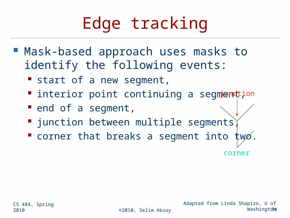
Edge tracking
Mask-based approach uses masks to identify the following events: start of a new segment, interior point continuing a segment, end of a segment, junction between multiple segments, corner that breaks a segment into two.
junction
corner
Adapted from Linda Shapiro, U of Washington

CS 484, Spring 2010 ©2010, Selim Aksoy 75
Edge tracking: ORT Toolkit Designed by Ata Etemadi. The algorithm is called Strider and is like a spider
moving along pixel chains of an image, looking for junctions and corners.
It identifies them by a measure of local asymmetry. When it is moving along a straight or curved segment with
no interruptions, its legs are symmetric about its body. When it encounters an obstacle (i.e., a corner or junction)
its legs are no longer symmetric. If the obstacle is small (compared to the spider), it soon
becomes symmetrical. If the obstacle is large, it will take longer.
The accuracy depends on the length of the spider and the size of its stride.
The larger they are, the less sensitive it becomes.
CS 484, Spring 2010 ©2010, Selim Aksoy 76
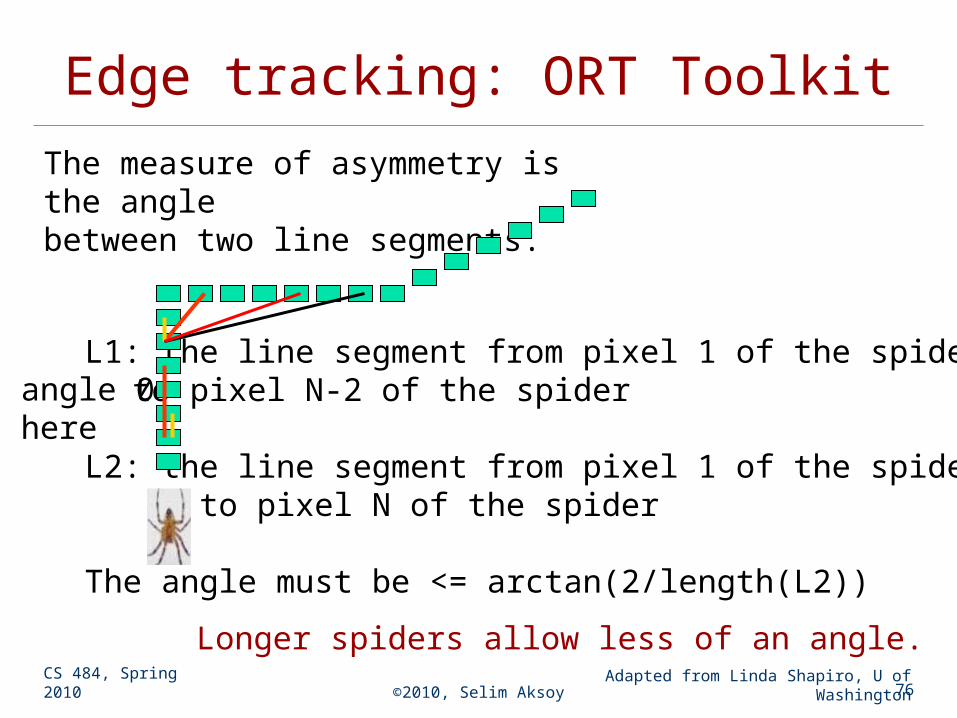
Edge tracking: ORT Toolkit
L1: the line segment from pixel 1 of the spiderto pixel N-2 of the spider
L2: the line segment from pixel 1 of the spider to pixel N of the spider
The angle must be <= arctan(2/length(L2))
angle 0here
The measure of asymmetry is the anglebetween two line segments.
Longer spiders allow less of an angle. Adapted from Linda Shapiro, U of
Washington
CS 484, Spring 2010 ©2010, Selim Aksoy 77
Edge tracking: ORT Toolkit The parameters are the length of the spider
and the number of pixels per step. These parameters can be changed to allow
for less sensitivity, so that we get longer line segments.
The algorithm has a final phase in which adjacent segments whose angle differs by less than a given threshold are joined.
Advantages: Works on pixel chains of arbitrary complexity. Can be implemented in parallel. No assumptions and parameters are well
understood.

CS 484, Spring 2010 ©2010, Selim Aksoy 78
Example: building detection
by Yi Li @ University of Washington

CS 484, Spring 2010 ©2010, Selim Aksoy 79
Example: building detection

CS 484, Spring 2010 ©2010, Selim Aksoy 80
Example: object extractionby Serkan Kiranyaz
Tampere University of Technology

CS 484, Spring 2010 ©2010, Selim Aksoy 81
Example: object extraction

CS 484, Spring 2010 ©2010, Selim Aksoy 82
Example: object extraction

CS 484, Spring 2010 ©2010, Selim Aksoy 83
Example: object extraction

CS 484, Spring 2010 ©2010, Selim Aksoy 84
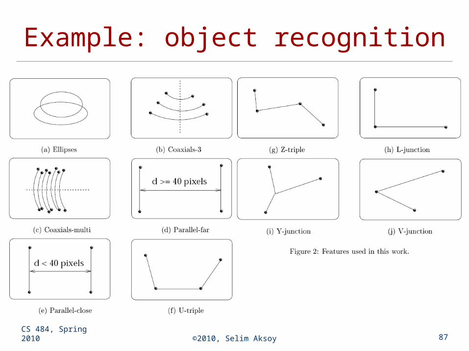
Example: object recognition
Mauro Costa’s dissertation at the University of Washington for recognizing 3D objects having planar, cylindrical, and threaded surfaces: Detects edges from two intensity images. From the edge image, finds a set of high-level
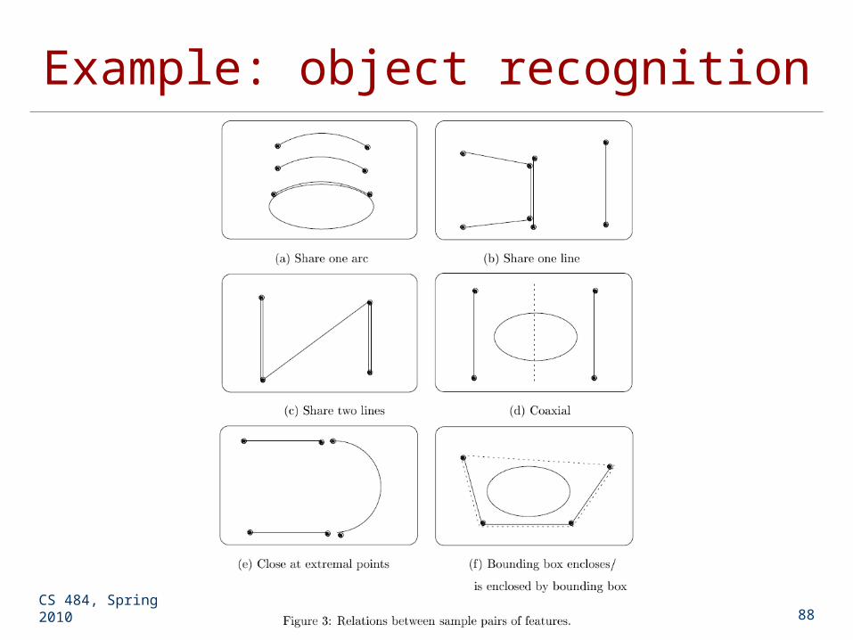
features and their relationships. Hypothesizes a 3D model using relational
indexing. Estimates the pose of the object using point
pairs, line segment pairs, and ellipse/circle pairs. Verifies the model after projecting to 2D.
CS 484, Spring 2010 ©2010, Selim Aksoy 85
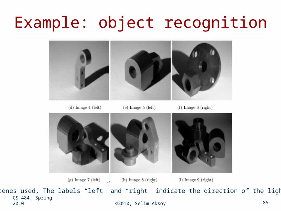
Example: object recognition
Example scenes used. The labels “left” and “right” indicate the direction of the light source.

CS 484, Spring 2010 ©2010, Selim Aksoy 86
CS 484, Spring 2010 ©2010, Selim Aksoy 87
Example: object recognition
CS 484, Spring 2010 ©2010, Selim Aksoy 88
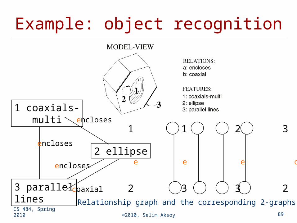
Example: object recognition
CS 484, Spring 2010 ©2010, Selim Aksoy 89
Example: object recognition
1 coaxials-multi
3 parallellines
2 ellipseencloses
encloses
encloses
coaxial
1 1 2 3
2 3 3 2
e e e c
Relationship graph and the corresponding 2-graphs.

CS 484, Spring 2010 ©2010, Selim Aksoy 90
Example: object recognition
Learning phase: relational indexing by encoding each 2-graph and storing in a hash table.
Matching phase: voting by each 2-graph observed in the image.
CS 484, Spring 2010 ©2010, Selim Aksoy 91
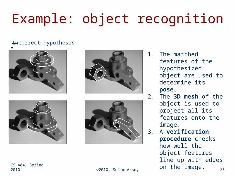
Example: object recognition
1. The matched features of the hypothesized object are used to determine its pose.
2. The 3D mesh of the object is used to project all its features onto the image.
3. A verification procedure checks how well the object features line up with edges on the image.
Incorrect hypothesis