UNIVERSIDADE DE LISBOA

FACULDADE DE CIÊNCIAS

DEPARTAMENTO DE BIOLOGIA ANIMAL

Ecosystem Services in urban areas: evaluating the role of green

spaces to improve air quality using ecological indicators

Mestrado em Ecologia e Gestão Ambiental

Joana Isabel de Figueiredo Vieira

Dissertação orientada por:

Doutora Cristina Branquinho e Doutor Pedro Pinho

2015

Agradecimentos

Obrigada aos meus orientadores: Dr.ª Cristina Branquinho e Dr. Pedro Pinho,

pela confiança e entusiasmo desde o primeiro minuto. Foi um privilégio dar

os primeiros passos na investigação com a vossa supervisão. A paixão pela

ciência que demonstraram foi contagiante, levo-a para a vida.

À Paula Matos um especial obrigado por todo o apoio e paciência com as

identificações. E pela preciosa ajuda mesmo no final!

Muito obrigada a todo o grupo do CE3C pela receção calorosa e por toda a

aprendizagem proporcionada ao longo deste ano. Ana Cláudia, Adriana, Alice,

Artur, Cristina, Mélanie, Helena, João, Teresa, Paula Gonçalves, Silvana,

Ricardo e Sérgio, obrigada pela boa-disposição, amizade e disponibilidade em

ajudar.

A todos os meus amigos um obrigado carinhoso. Em especial aos que tornam

este ano inesquecível, Cláudia, Daniela T, Daniela C, Filipa, Frederico e Joana;

Aos oliveirenses das cafezadas, pelos momentos únicos; E aos amigos do

coração Berta, Patrícia e Pedro, por tudo.

À minha família, que é grande mas cabe toda dentro do coração, um obrigada

ainda maior. Em especial à minha mãe, ao meu pai, à minha irmã e ao Jorge.

Sem vocês esta tese não seria possível, nem faria sentido.

Index

1. Introduction ................................................................................ 1

2. Methods ....................................................................................... 5

2.1 Study area ................................................................................ 5

2.2 Sampling design ......................................................................... 5

2.3 Data collection ........................................................................ 7

2.3.1 Lichen sampling .................................................................... 7

2.3.2 Environmental variables......................................................... 8

2.3.4 PM10 data ............................................................................... 11

2.4 Lichen functional diversity .......................................................... 11

2.5 Data analysis ............................................................................ 12

2.6 Software used ........................................................................... 14

3. Results ........................................................................................ 15

3.1 Green spaces and total lichen diversity metrics characterization ...... 15

3.2 Lichen functional diversity metrics ............................................... 17

3.3 Explaining biodiversity patterns ................................................... 18

3.4 Lichens richness model for green spaces ...................................... 23

3.5 Applying the lichens species richness model to other green spaces .. 27

3.6 Risk maps for health problems associated with air quality ............... 30

4. Discussion .................................................................................. 35

4.1 The patterns of lichen diversity in Lisbon green spaces ................... 35

4.2 Factors affecting air quality in green spaces .................................. 38

4.3 The role of Lisbon gardens in air purification ................................. 41

4.4 Air quality in Lisbon: focusing on risk areas for humans ................. 42

5. Final remarks .............................................................................. 43

References ...................................................................................... 45

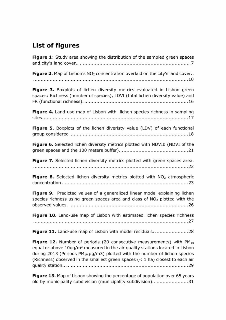
List of figures

Figure 1: Study area showing the distribution of the sampled green spaces

and city’s land cover.. ......................................................................... 7

Figure 2. Map of Lisbon’s NO2 concentration overlaid on the city’s land cover..

....................................................................................................... 10

Figure 3. Boxplots of lichen diversity metrics evaluated in Lisbon green

spaces: Richness (number of species), LDVt (total lichen diversity value) and

FR (functional richness). ..................................................................... 16

Figure 4. Land-use map of Lisbon with lichen species richness in sampling

sites ................................................................................................. 17

Figure 5. Boxplots of the lichen diveristy value (LDV) of each functional

group considered ............................................................................... 18

Figure 6. Selected lichen diversity metrics plotted with NDVIb (NDVI of the

green spaces and the 100 meters buffer). . ........................................... 21

Figure 7. Selected lichen diversity metrics plotted with green spaces area.

....................................................................................................... 22

Figure 8. Selected lichen diversity metrics plotted with NO2 atmospheric

concentration .................................................................................... 23

Figure 9. Predicted values of a generalized linear model explaining lichen

species richness using green spaces area and class of NO2 plotted with the

observed values. ............................................................................... 26

Figure 10. Land-use map of Lisbon with estimated lichen species richness

....................................................................................................... 27

Figure 11. Land-use map of Lisbon with model residuals. ...................... 28

Figure 12. Number of periods (20 consecutive measurements) with PM10

equal or above 10ug/m3 measured in the air quality stations located in Lisbon

during 2013 (Periods PM10 μg/m3) plotted with the number of lichen species

(Richness) observed in the smallest green spaces (< 1 ha) closest to each air

quality station.. ................................................................................. 29

Figure 13. Map of Lisbon showing the percentage of population over 65 years

old by municipality subdivision (municipality subdivision).. ..................... 31

Figure 14. Map of Lisbon with the percentage of population under 14 years

old by municipality subdivision.. .......................................................... 32

Figure 15. Average lichen species richness estimated for Lisbon at the parish

level (Richness) plotted with the percentage of elderly people (>65 years old)

in the same subdivision (% elderly).. ................................................... 33

Figure 16. Average species richness estimated for Lisbon at the parish level

(Richness) plotted with the percentage of younger population (0-14 years

old) in the same municipality subdivision (% children). .......................... 33

Figure 17. Health risk map for elderly people (> 65 years old) by parish. 34

Figure 18. Health risk map for children (< 14 years old) by parish.. ....... 35

List of tables

Table 1. Traits and related functional groups following Nimis & Martellos

2008.. .............................................................................................. 12

Table 2. Descriptive statistics of environmental and biodiversity variables

analyzed. .......................................................................................... 15

Table 3. Spearman correlation coefficients between environmental

variables and lichen biodiversity metrics. .............................................. 20

Table 4. Summary of the Generalized Linear Models (GLMs) explaining the

effects of environmental variables on lichen species richness.. ................ 24

Table 5. Regression results obtained by a generalized linear model

explaining lichen species richness using green spaces area and class of NO2

atmospheric concentration.. ................................................................ 25

Table 6. Statistics for the observed and predicted values obtained by cross-

validation of a generalized linear model explaining lichen species richness

using green spaces area and class of NO2 atmospheric concentration.. ..... 25

Table 7. Effect of 10 % increase of green spaces area in lichens species

richness.. .......................................................................................... 30

Abstract

Air pollution has substantial impacts in human health. The air quality policies

implemented in Europe during the last decades led to an overall decrease in

pollution originated from industry. However, in general in urban areas traffic

intensity is still significant, exposing urban citizens to various air pollutants.

In face of the expected increase in the number of people living in cities, from

current 54% to 66% in 2050, management actions to improve air quality in

urban areas are imperative.

Urban green spaces are known to provide several ecosystem services, namely

those associated to air purification. However, the quantification of this

ecosystem service is still undone. Quantifying the role of green spaces in air

purification requires information with high spatial and temporal resolution.

Air quality monitoring stations in cities are scarce, due to their elevated costs,

and the existent ones are far from providing an adequate spatial cover. The

lack of air quality data with high spatial resolution and with consistent time-

series matching the diversity of green space typologies, have been the main

setback for this ecosystem service evaluation.

Ecological indicators are good candidates for monitoring ecosystem services

in urban areas. Lichens are within the most widely used ecological indicators

to monitor air quality, including in urban areas, due to their direct dependence

of atmospheric conditions. They can be sampled in a flexible way in urban

areas, providing high spatial resolution data and integrating the time

component.

The aim of this study was to evaluate and model how green spaces can

improve air quality in urban areas, using lichen as ecological indicators. The

work was performed in Lisbon, a large city with multiple typologies of green

spaces, and areas with variable atmospheric pollution levels. Lichen diversity

was sampled following the standard European method in 42 green spaces

stratified by size and location. Other environmental variables associated with

green spaces and its surroundings were evaluated, such as vegetation density

and surrounding urban density.

Lichen species richness in green spaces was very significantly related with

most variables associated to air quality. Thus, this simple and very robust

metric was selected as ecological indicator of the effects of air quality in cities.

Background pollution, likely from traffic, contributed to decreasing air quality.

Conversely, high vegetation density in and around green spaces and large

green spaces contributed positively to air quality in Lisbon green spaces.

A model for air quality on Lisbon green spaces allowed us to determine that

increasing their area or building small gardens greatly contributes for

improving local air quality. Low air quality is an additional health risk for

Lisbon population, particularly for the most vulnerable groups, such as elderly

people (>65 years) and children (>14 years). Using the same model, we

provided a health risk map for the most susceptible age groups of the

population: elderly and children. Ultimately, this framework can be used as a

tool for informed decisions in urban green spaces management aiming at air

purification using ecosystem services.

Keywords: Lisbon, air pollution, gardens, lichens, green urban management

Resumo

O número de pessoas a viver em cidades tem vindo a aumentar, tornando

cada vez mais importante a questão da poluição associada às áreas urbanas.

Os espaços verdes citadinos constituem zonas de lazer e de redução do

stress, estando associados a diversos serviços do ecossistema,

nomeadamente, a diminuição da poluição do ar. A densidade de árvores e o

tamanho do espaço verde são geralmente considerados como muito

importantes para esta capacidade. No entanto, há ainda um número reduzido

de estudos que abordem os espaços verdes urbanos, principalmente os de

pequena dimensão.

Este trabalho teve como objetivo analisar a importância dos espaços verdes

na diminuição da poluição do ar em zonas urbanas. Com esse intuito

construiram-se modelos de qualidade do ar para os espaços verdes utilizando

indicadores ecológicos. Este trabalho foi desenvolvido em Lisboa, a maior

cidade de Portugal, situada no centro do país. Este revelou-se um bom local

de estudo devido à alta concentração de poluentes urbanos, ao elevado

número de habitantes e à existência de uma grande diversidade de áreas

verdes, principalmente nas áreas menos centrais. A quantificação da

qualidade do ar nos espaços verdes desta cidade poderá contribuir para uma

gestão mais eficaz e ponderada destes.

A amostragem de espaços verdes foi feita de forma aleatória e estratificada

à zona, à área e à densidade de tecido urbano envolvente, de forma a não

subamostrar zonas com menos espaços verdes, espaços verdes de dimensões

elevadas ou com tecido urbano pouco denso. A amostragem de líquenes foi

realizada em 42 espaços de verdes. Em cada espaço verde a diversidade de

líquenes epífitos foi analisada nas 4 árvores mais próximas do centróide

possível. Foi registada a frequência das espécies encontradas, seguindo um

protocolo europeu standard. Quando a identificação no local não foi possível,

foram recolhidas amostras para posterior identificação em laboratório. Foi

ainda registado o diâmetro à volta do peito de cada árvore amostrada.

Foram tidas em conta várias métricas de biodiversidade: o valor de

diversidade de líquenes (LDV), a riqueza, a riqueza funcional (FR). Foi

calculada a área total de cada espaço verde e o NDVI (normalized diference

vegetation index) do centróide de cada espaço verde e do conjunto do espaço

verde com um buffer de 100 metros em redor. As áreas foram obtidas através

da análise de fotografias aéreas e os valores de NDVI através de imagens do

satélite Landsat 8. Com o objetivo de ter em consideração a poluição de fundo

do tráfego automóvel, foram utilizados dados das concentrações de dióxido

de azoto (NO2) existentes nas diferentes zonas da cidade, calculadas num

trabalho anterior.

As espécies de líquenes identificadas foram caracterizadas em diferentes

grupos funcionais, de acordo com três atributos (traits): Tolerância à

eutrofização, requisitos de humidade e forma de crescimento.

Por fim, foram recolhidos dados relativos à população da cidade, tendo em

conta a faixa etária das respetivas freguesias. Os dados respeitantes à

população com menos de 14 anos e com mais de 65 anos foram

posteriormente tidos em conta para a produção de mapas de risco, tendo em

conta a maior suscetibilidade à poluição destas faixas etárias.

O tratamento estatístico inicial dos dados envolveu a realização de

coeficientes de correlação de spearman entre as variáveis ambientais e as

métricas consideradas. Posteriormente foram elaborados modelos (GLM)

tendo em conta apenas as variáveis com maiores associações. O modelo final

foi selecionado tendo em conta o princípio da parcimónia e o maior valor de

AIC. De seguida, o modelo, que tem como variáveis explicativas a área do

espaço verde e a concentração de NO2, foi aplicado a 63 espaços verdes de

Lisboa, para além dos realizados da amostragem inicial.

A métrica de biodiversidade Riqueza foi a que apresentou maiores

associações com as variáveis ambientais. Assim, esta métrica, fácil de aplicar

e muito robusta, foi utilizada como indicadora da qualidade do ar nos espaços

verdes de Lisboa.

Os resultados obtidos sugerem que o NDVI do espaço verde e a área deste

são fatores preponderantes para a qualidade do ar em espaços verdes

urbanos. Também a poluição de fundo (provavelmente com origem

automóvel) é de grande importância para a qualidade do ar nestes espaços.

Estas foram as variáveis ambientais com maior correlação com as métricas

consideradas.

No total dos espaços amostrados foram identificadas 22 espécies, valores

semelhantes aos apresentados na bibliografia para outras cidades europeias.

Em relação a um estudo anterior nos anos 70, a qualidade do ar em Lisboa

aparenta não ter sofrido grandes alterações, o que se poderá dever à

diminuição dos poluentes emitidos por veículo, devido aos avanços

tecnológicos, em simultâneo com o aumento do número de veículos em

circulação desde os anos 70. No entanto, as diferenças no tipo de

amostragem poderão ser relevantes e justificar estes valores. Relativamente

aos grupos funcionais considerados, os líquenes xerófitos, oligotróficos e

nitrófilos foram os obtidos em maior número, enquanto os fruticosos foram

os menos abundantes.

Foi ainda comparada a riqueza de líquenes, nos espaços verdes mais

próximos das estações de qualidade do ar existentes em Lisboa, com as

medições de PM10 no ano de 2013 em cada uma dessas estações. A riqueza

de líquenes mostrou estar significativamente correlacionada com o número

de períodos (20 dias consecutivos) de partículas acima dos 10ug/m2.Esta

correlação linear permitiu-nos utilizar a riqueza de líquenes como um

sorrugate da qualidade do ar dos espaços verdes.

Analisando o modelo obtido neste trabalho foi ainda possível estimar a

melhoria do ar nos espaços verdes de Lisboa. Assim, inferiu-se que o mesmo

aumento de área em espaços verde de dimensões pequenas é mais eficaz na

redução da poluição do ar que em espaços verdes de grandes dimensões. Por

exemplo, com 10% de aumento de área, num espaço verde de 300m2 pode-

se alcançar 14% de melhoria da qualidade do ar enquanto num espaço verde

com 50000m2 a melhoria ronda os 1,5%. Também foi possível verificar que

em zonas com mais poluição de fundo a melhoria é mais potenciada do que

em zonas com menos poluição de fundo.

Da análise da população das diferentes freguesias em Lisboa, concluiu-se que

é na zona centro que existe as freguesias com maior percentagem de idosos

e na periferia as freguesias com maior percentagem de crianças. De salientar,

que a percentagem de idosos é bastante superior à de crianças e por isso

estes devem ser tidos em conta mais atentamente. A zona central da cidade

é também onde os espaços verdes possuem pior qualidade do ar, estimada

pelo modelo criado neste trabalho. Assim, esta é uma zona que requer

especial atenção por parte dos gestores dos espaços verdes. A criação de

espaços verdes com maior tamanho e densidade de árvores ou a ampliação

e readaptação de espaços verdes existentes são duas ações sugeridas. Em

situações de elevada densidade urbana, os telhados e as paredes verdes são

boas possibilidades. Tendo em conta a influência do trafego automóvel na

poluição dos espaços verdes, é também sugerido medidas como, por

exemplo, a diminuição de duas vias para uma só, substituindo a segunda por

uma linha de árvores.

Palavras-chave: Líquenes, qualidade do ar, áreas urbanas, espaços verdes

Abbreviation list

DBH - Diameter at breast height

LDV - Lichen Diversity value

FR - Functional richness

NDVI - Normalized Difference Vegetation Index

PSR - Potential solar radiation

NO2 - Nitrogen dioxide

GLM - Generalized Linear Model

AIC - Akaike’s Information Criterion

Slop - Slope

Alt - Altitude

Dist - Distance from the coast line

PM10 - Particulate matter up to 10 micrometers in size

1

1. Introduction

Currently, more than half of world’s population lives in cities and by 2050 this

number is expected to increase by 66 percent (United Nations [UN], 2014).

The fast and unprecedented cities’ growth brought severe challenges to

society, including environmental degradation, loss of natural habitat, and

increased human health risks associated with heat, noise and pollution

(Zupancic et al., 2015).

Despite the progress made in Europe during the last decades to implement

strict air policies, substantial problems of air quality remain (European

Environmental Agency [EEA], 2014), particularly in urban areas. The levels

of classical and very toxic air pollutants such as sulphur dioxide from

industrial emissions have substantially decreased. However, as a

consequence of traffic, urban citizens remain exposed to various air pollutants

such as nitrogen oxides, volatile organic compounds, particulate matter and

photochemical oxidants (Fenger, 2009). Air pollution costs both money and

health to city’s inhabitants. Estimations show that in 2012 more than 400 000

premature deaths were attributable to air pollution in Europe (World Health

Organization [WHO], 2014). In Portugal alone, the economic costs of deaths

from air pollution in 2010 were estimated to be around 8,5 million euros, half

of which associated to air pollution derived from road transport (WHO, 2014).

In the same year, 38 003 deaths in Portugal were attributed to air pollution

(Organisation for Economic Co-operation and Development [OECD], 2014).

It is clear that air pollution in cities represents a serious environmental

problem and its mitigation a major public challenge. Therefore, improving air

quality has substantial, quantifiable and important civic health benefits (Chen

& Kan, 2008).

Within human population, some age groups show a higher vulnerability to air

pollution. Higher health risks were demonstrated in the elderly (> 65 years),

when comparing to the rest of the population. For instance, increased

pollution exposure in the elderly was associated with increased mortality by

cardiopulmonary or respiratory causes and with an increased number of

2

hospital admissions and emergency-room visits (Simoni et al., 2015).

Children (< 14 years old) may also have a greater potential for adverse health

effects, when compared to adult population. Children’s ongoing development

makes them more susceptible, and differences in their metabolism and

behavior may cause them to reach higher levels of exposure when exposed

in the same environment as adults (Selevan et al., 2000).

Ecosystem based solutions can be used to improve air quality in a cost-

effective way, and can work synergistically with more demanding air policies.

Ecosystem services can be defined as the benefits human populations derive

from ecosystem functions, directly or indirectly (Costanza et al., 1997). Green

spaces provide numerous ecosystem services in urban areas: air filtration,

microclimate regulation, noise reduction, rainwater drainage, recreational

and cultural values, among others (Bolund & Hunhammar, 1999; Jansson et

al., 2014). For example, a study in the UK showed that a 10 percent

increase in tree cover in mid-size cities could increase about 12 percent of

the existing vegetation carbon stock (Davies et al, 2011). Urban green spaces

also play an important role in the lives of people inhabiting cities, such as

reducing stress (Ulrich et al., 1991) and restoring the capacity of citizens to

focus (Berto, 2005), among others. Morancho (2003) showed an inverse

relationship between the selling price of a residence and its distance from an

urban green space. This hedonic valuation suggests that people have a

preference for living next to green spaces. Decision-makers and politicians

are progressively aware of the importance of urban ecosystem services for

human health and well-being in cities. However, the way to measure the

benefit of those services with high spatial resolution for decision-making

remains an open question (Lakes & Hyun-Ok, 2012). This is especially

relevant for air quality, which can change radically over very short distances.

Thus, an open question remains, how much can a green space produce the

service of air purification?

It is already known that green spaces can purify air both by direct and indirect

mechanisms. Directly, through the filtering effect of plants, mainly based on

dry deposition of pollutants through stomata uptake or non-stomatal

deposition on plant surfaces (Gheorghe & Ion, 2011). Indirectly, mainly by

improving urban ventilation, which in turn amplifies the dispersal of the

3

pollutants (Givoni, 1991). Although vegetation can purify the air, the extent

of that reduction depends on local conditions (Svensson & Eliasson, 1997).

For instance, it was shown that higher densities of tree canopies in forest

parks decrease PM10 concentration inside them (Cavanagh et al., 2009).

However, this study was based on a single urban green space. Bowler et al.

(2010) identified gaps in the literature that include shortage of data on the

optimal size, allocation and characteristics of the green spaces that can

contribute to improve urban areas for human health, namely in reducing

human exposure to ground level ozone concentrations. A recent systematic

review found only a few studies on the mitigation of pollution impacts by

small urban parks (Zupancic et. al, 2015). But importantly, among all works

reviewed, all types of green spaces were positively related with air

purification, from small green walls to large-scale urban forests.

To study how green spaces purify the air, long-term measures of atmospheric

pollutants should be used. However, only a few air quality stations are

available due to its high operating costs. As a consequence, the available air

quality data has insufficient spatial resolution, and those stations are rarely

associated to green spaces. As an example, in the city of Lisbon only 6

stations are operating, and measuring a limited number of pollutants. The

most recent station is available only since 2000 and not all stations measure

the same pollutants. The low number of stations translated in a lack of high

spatial and temporal resolution, make it extremely difficult to understand the

role of green spaces in purifying air in cites.

A solution to overcome this problem is the use of ecological indicators. They

allow measuring the effect of green spaces on air pollution reduction, by

retrieving information with high spatial resolution and in a flexible way.

Ecological indicators can be used to assess the condition of the environment

or to monitor trends in condition over time, to provide an early warning signal

of changes in the environment, or to diagnose the cause of an environmental

problem (Dale & Beyeler, 2001). An ecological indicator can be included under

the concept of surrogate, which is a component of the system of concern that

can be more easily assessed or managed than others, and that is used as an

indicator of, for instance, the quality of that system (Mellin et al., 2011; Caro

et al., 2010; Lindenmayer et al., 2015).

4

Lichens are a symbiotic association between a fungus and an algae and/or

cyanobacteria (Honegger, 1991). Lichens lack roots, taking up water, solutes

and gases over the entire thallus surface, and so depending on the

atmosphere for nutrition (Hauck, 2010). Moreover, their lack of cuticle and

stomata means that the different contaminants are absorbed over the entire

surface of the organism (Hale, 1983). Consequently, lichens have been

extensively used for monitoring air quality as they respond to atmospheric

pollutants directly, being defined as “permanent control systems” for air

pollution assessments (Nimis et al., 1989; 2002). Lichens were used as

ecological indicators in physiological studies, as bioaccumulators of

pollutants, and in biodiversity studies, since species show different

sensibilities to air pollutants (Branquinho, 2001). For instance, in the

Portuguese city Almada, lichens showed to be related to the city’s

microclimatic gradient, and its functional diversity regarding water

requirements responded in an integrated way to the climatic modifications

occurring in the city, namely the heat island effect (UHI) and the alleviation

effect of forested areas (Munzi et al., 2014).

Several biodiversity metrics using lichens can be applyed when analyzing air

quality, such as total diversity or functional diversity, by means of functional

traits and functional groups (Nimis et al., 2002). Both measures of total

diversity and functional diversity were already used to evaluate the effects of

environmental change in ecosystems (Giordani, Brunialti & Alleteo, 2002;

Pinho et al., 2011; Pinho et al., 2012; Pinho et al, 2014). Total diversity

metrics include species richness (the number of species) and the lichen

diversity value, LDV (a measure of species frequency) (Asta et al., 2002);

while functional diversity metrics (the diversity of species traits in

ecosystems), can include measures of functional richness (Schleuter, 2010)

or the LDV of each functional group (Pinho, 2009). Functional richness can be

measured as the number of functional groups (Villeger & Mouillot, 2008).

Functional traits are the characteristics of an organism that are considered

significant to its response to the environment and/ or its effects on ecosystem

functioning (Diaz & Cabido, 2001). Functional groups are composed by a set

of species with either similar responses to the environment or similar effects

on major ecosystem processes (Gitay & Noble, 1997). An example could be

5

the lichen response trait “tolerance to drought” and its division into

hygrophyte and xerophyte functional groups (Llop et al., 2012).

Nevertheless, the most reliable metrics to be used in urban areas and the

way atmospheric pollution affects them remains largely unstudied (Davis et

al., 2007).

The aim of this work was to evaluate and model with high spatial resolution

the role of green spaces in improving urban air quality. We used lichens as

ecological indicators of atmospheric pollution, using several metrics of

biodiversity measured in green spaces with different characteristics (size,

surrounding urban density, vegetation density). Finally, we intended also to

make a health risk assessment, at the parish size, for the most susceptible

age groups of the population, the elderly and children. Increasing the capacity

to minimize air pollution using green spaces would be a great contribution to

citizens. Therefore, this work also aims to propose management practices

oriented to increase green spaces capacity to purify air.

2. Methods

2.1 Study area

This work was done in Lisbon, a city located on the western coast of Portugal,

on the right bank of the Tagus River. Lisbon has a population of 2821876

residents in its metropolitan area (Instituto Nacional de Estatística [INE],

2011). This city is characterized by a Mediterranean climate, with an annual

mean temperature of 17,1°C and mean annual precipitation of 788,3 mm

(1960-2014 average; Base de Dados de Portugal Contemporâneo

[PORDATA], 2015), with north and north-western prevailing winds.

2.2 Sampling design

6

Prior to the selection of sampling sites, a complete cartography of Lisbon’s

green spaces was done. As the European Urban Atlas contemplates only large

green spaces (>1 ha), smaller green spaces were added to the cartography

by manual photo interpretation of aerial photographs. From all existing green

spaces, a sub-sample was selected in a randomly stratified way. Sites were

stratified by location, urban density and green space area. This was done to

prevent oversampling the most frequent green spaces, i.e. those located in

city periphery, surrounded by low density urban areas and with small size.

For stratification by location, the city was divided into four quadrants (Figure

1), each with a similar number of green spaces. In each of these four

quadrants, green spaces were distributed into five classes considering the

histogram of all green spaces area. The following classes were considered: 0-

0.1, 0.1-0.5, 0.5–10, 10-40, and higher than 40 ha. Stratification by urban

density considered 100 meters buffers around each green space and high

resolution land cover information for each buffer was retrieved from the

European Urban Atlas. The following land cover categories were considered

to classify the area surrounding green spaces as high density: continuous

urban fabric; industrial, commercial, public, military and private units;

discontinuous dense urban fabric. The remaining land cover categories in the

area surrounding green spaces were considered as low density. Finally, for

each class of area within each quadrant, two green spaces were randomly

chosen, one with surrounding high urban density and another with

surrounding low urban density (N=40). After this selection another two green

spaces were added: Parque florestal de Monsanto (by far the largest green

space in the city, two orders of magnitude larger than the others) and Avenida

da Liberdade (considered the most polluted area in Lisbon). As a result, a

total of 42 sampling sites were selected.

7

Figure 1: Study area showing the distribution of the sampled green spaces

(N=42) and city’s land cover. Dashed lines divide the study area in the four

quadrants considered for the stratification by location.

2.3 Data collection

2.3.1 Lichen sampling

Epiphytic lichen diversity was surveyed in the four suitable trees closest to

the centroid of each green space. The centroid of each green space is the

most comparable point between all green spaces, as it is always the most

protected place (Hamber et al., 2008) and, therefore, the one with higher

potential for air pollution reduction.

The enormous diversity of tree species in Lisbon green spaces prevented the

use of a single phorophyte, as suggested in by the sampling method (Asta et

8

al., 2002). To minimize the potential confounding factors caused by this, only

phorophytes with medium bark roughness were selected.

Tree selection followed standard conditions: trunk inclination with a deviation

from vertical inferior to ten degrees; circumference at breast height higher

than 50 cm; with a clear area on the trunk at this height, without damage,

decortication, branching, knots, or other epiphytes preventing lichen growth.

A grid with five squares, each with 10 x 10 cm, was attached to the trunk of

each tree at the four main cardinal points, of the lowermost part at 1 m above

ground, adapting the sampling procedure of the standard European protocol

(Asta et al., 2002). Each lichen species occurring inside each grid cell was

identified and recorded, or collected for later laboratory identification. Lichen

species frequency was recorded as the number of grid cells (out of 20

possible) where each species was detected.

Lichen species richness was calculated as the total number of species in each

green space. Lichen Diversity Value (LDV) was calculated for each tree as the

sum of all species frequencies. The species frequency and the LDV of each

green space (LDVt) represent the average of the four sampled trees.

Species nomenclature follows Nimis & Martellos (2008). Tree diameter at

breast height and the GPS coordinates of each tree were recorded.

2.3.2 Environmental variables

The Normalized Difference Vegetation Index (NDVI) is used to estimate

vegetation density and condition, being one of the most widely used

vegetation-related metrics (Bernan et al, 2011). NDVI values range from -1

to +1, with negative values corresponding to an absence of vegetation

(Myneni et al., 1995). To estimate the density of the vegetation in each green

space and in the surrounding 100 meters, satellite images taken from Landsat

8 (30 meters resolution) in May 2015 were analysed using the reflectance of

bands 5 and 4, corresponding to the near infrared and visible. The reflectance

of the two bands was calculated according to the following formula, where

Ρλ= Top of atmosphere planetary reflectance, θe = Local sun elevation angle,

M 𝜌 = Band-specific multiplicative rescaling factor from Landsat metadata, A 𝜌

9

= Band-specific additive rescaling factor from Landsat metadata and Qcal =

Quantized and calibrated standard product pixel values.

𝜌𝜆 =𝑀𝜌 × 𝑄𝑐𝑎𝑙 + 𝐴𝜌

sin(𝜃𝑒)

NDVI was calculated using bands reflectance, using the following index.

𝑁𝐷𝑉𝐼 =(𝑁𝐼𝑅 − 𝑅𝐸𝐷)

(𝑁𝐼𝑅 + 𝑅𝐸𝐷)

Afterwards, the average NDVI of the green space, and in the surrounding 100

meters buffer, was determined and used in subsequent analysis.

Each green space was analysed by manual photo interpretation of aerial

photographs to calculate the percentage of area in each green space that was

covered by buildings, pavements or areas with no vegetation (NVeg).

Urban density around each green space was also calculated for both 50 and

200 meters buffers, using the land cover categories considered to classify the

area surrounding green spaces in the 100 meter buffers (see 2.2 Sampling

design; U50, U100 and U200).

The average altitude (m), slope (º) and potential solar radiation (Wh/m2, used

here as a surrogate of local microclimate) were calculated from a digital

elevation model, derived from hypsometric curves with 10 meters interval.

The Euclidian distance to the river was obtained using the information

provided in the national database Atlas da Água.

A map of NO2 concentration in the city of Lisbon (Mesquita, 2009) was used

to estimate air pollution at each green space. The map was interpolated by

ordinary kringing of measured NO2 concentrations in 2002 and 2003.

Concentration values were retrieved from air quality stations and diffusion

tubes distributed across the city. Based on this information, we built a map

with four classes of NO2 concentration and the concentrations for each green

space was determined (Fig. 2). For all analysis we report the classes using

the values from 1 (to the lower concentration class) to four (to the high

concentration class).

10

NO2, U50, U100 and U200 were considered as surrogates of anthropogenic

pressure (human activities which can generate air pollution), namely car

traffic and intensity of urban matrix use surrounding the green space.

Figure 2. Map of Lisbon’s NO2 concentration overlaid on the city’s land cover.

Four classes of NO2 concentration were considered : < 20 μg/m3 – class 1;

20 - 30 μg/m3 - class 2; 30 - 35 μg/m3 – class 3; >35 μg/m3 – class 4 (adapted

from Mesquita, 2009).

2.3.3 Demographic population data

Information on Lisbon population was collected by residence area and age.

Data was retrieved from last Census in the city (INE, 2011). It is important

to refer that when the Census information was compiled, city’s administrative

boundaries at the parish level were different from the current ones. To

preserve consistency, old Census boundaries at the parish level were

considered in all maps.

11

2.3.4 PM10 data

Data on atmospheric particulate matter inferior to 10 micrometers size (PM10)

was obtained from the environmental Portuguese agency online data base

QualAr (http://qualar.apambiente.pt/). The records include hourly

concentrations in five of the six stations located in Lisbon for 2013. Data were

treated in the following way. For each twenty sequential PM10 measures, the

number of measurements with 10 µg/m3 or more was recorded. At end of the

year we considered the number of 20 sequential measurements that were all

equal or above 10 µg/m3.

2.4 Lichen functional diversity

Lichen species were classified according to three response traits: humidity

requirements, type of growth form and eutrophication tolerance. Functional

group classification was based on the Italian database (Table 1; Nimis &

Martellos 2008).

Species functional group classification was combined with species frequency

data to obtain the LDV for each functional group at each green space. In

addition, functional richness (FR) was also calculated for the set of traits

growth form, humidity requirements and eutrophication tolerance. As these

traits are categorical, FR corresponds to the number of functional groups

present at each site.

12

Table 1. Traits and related functional groups following Nimis & Martellos

2008. Species maximum tolerance was considered for the humidity

requirements and eutrophication tolerance.

Trait Functional group Description

Humidity requirements

Hygrophytic

Mesohygrophytic Xerophytic

From high to rather high humidity

requirements

Medium humidity requirements

From low to rather low humidity requirements

Growth form

Crustose

Leprose

Squamulose

Foliose narrow-

lobed

Foliose broad-

lobed

Fruticose

Firmly and entirely attached to the substrate by the lower surface

Like crustose but surface thallus with a granular mass appearance and always

decorticated

Composed of small scales

Partly attached to the substrate with a leaf-like form and narrow lobes

Same as foliose narrow-lobed but with broad lobes

3D-like structure, attached by one point to the substrate and with the rest of the thallus

protruding from the surface of the substrate

Eutrophication

tolerance

Nitrophytic

Mesotrophic

Oligotrophic

From tolerant to high eutrophication to very high eutrophication

Weak eutrophication

From sensitive to eutrophication to very weak eutrophication tolerance

2.5 Data analysis

Spearman correlations between biodiversity metrics and environmental

variables were calculated to account for possible nonlinearity in the

relationships. Correlations were considered significant for P < 0.05. The

13

metrics and the environmental variables with higher correlations to

biodiversity variables were selected for further analysis. This analysis allowed

the selection of the most promising biodiversity metrics to be used as

ecological indicators of the pollution effects. It is important to refer that green

spaces area values were logarithmized prior to the analysis.

A General Linear Model (GLM) was used to predict air quality based on the

environmental variables. The selected lichen variable(s) were modelled with

the selected environmental predictors. The GLMs were popularized by

McCullagh and Nelder, 1989. In this type of models the relationship between

the response variable Y and the values of the X variables is assumed to be:

Y = b0 + b1X1 + b2X2 + ... + bkXk

In GLM the dependent variable does not need to be normally distributed and

normally distributed error terms are not assumed. Moreover, in STATISTICA

the GLM outline allows a simpler treatment of all possible predictor variables

combinations and a quick comparison of the various models. GLM models are

fitted via Maximum Likelihood estimation.

As pointed out by Burnham & Anderson (2001), three principles regulate our

ability to make inferences in science: simplicity and parsimony; several

working hypotheses; strength of evidence. The principle of parsimony was

used in the selection of the models. From the models built with the significant

variables, the selected model was chosen ensuring a small number of

variables with the highest Akaike Information Criterion (AIC) value. An effect

of interaction (first used by Fisher, 1926) occurs when a relationship between

two or more variables is modified by at least one other variable. Interactions

significance between the environmental variables was tested to assess if

those relationships were important in model construction.

The model cross-validation was performed by randomly partitioning the

original sample into 10 subsamples, with approximately 10% subsets of the

original values. The new model calculations were performed with the

remaining 90% observed values. Ten new equations were generated for the

model, which were then used to predict the values at the excluded points.

14

The results from the 10 subsamples were averaged to produce a single

estimation. Afterwards, the average difference between the predicted and the

observed values was compared.

In order to analyze the association between the lichens richness and the

green spaces air quality, the number of periods (20 consecutive days) with

PM10 above 10ug/m3, measured in the air quality stations over 2013, were

plotted with the number of lichen species observed in the small green spaces

(< 1 ha) closest to each air quality station.

The model was then used to test the effect of increasing 10% in the area of

the green spaces on lichen species richness. This was done using the model

previously developed (see Mesquita, 2009) fixing for 3 classes of NO2 (< 20

μg/m3, 20 - 30 μg/m3 and 30 - 35 μg/m3) present in Lisbon.

The selected model was applied to 63 unsampled green spaces across the

city to predict air quality in those spaces and also to the 42 previously

sampled, resulting in more than 100 green spaces considered. Finally, health

risk maps were built joining demographic population data for each Lisbon

parishes and the averaged estimated lichen species richness of the green

spaces in the same subdivisions. Parishes with simultaneously low lichen

species richness and high percentage of vulnerable population (elder people

and children) were considered as high risk. Subdivisions with high lichen

diversity (more than 8 species) were considered as low risk independently of

the percentage of vulnerable population. The remaining subdivisions were

considered as medium risk.

2.6 Software used

Statistical analyses were performed with STATISTICA v12 (StatSoft, Inc.).

Maps were built using QGIS geographic information software v2.4.0 (QGIS,

Inc.). Functional richness (FR) was calculated using the ‘dbFD’ function of the

CRAN software R (R Core Team 2013) FD package (Laliberte & Legendre

2010).

15

3. Results

3.1 Green spaces and total lichen diversity metrics characterization

Lisbon green spaces areas ranged in three orders of magnitude from 287,21

m2 to 228 365,10 m2 (N=42; SD= 52 567,97; Table 2) without considering

Monsanto, the largest of them all with an area of 1,12E7 m2.

Table 2. Descriptive statistics of environmental and biodiversity variables

analyzed. Environmental variables: Alt (altitude), Arealog (green space

logarithmized area), DBH (diameter at breast height), U50/100/200

(percentage of high urban density in 50/100/200 m buffer surrounding the

green space), NO2 (class of NO2 atmospheric concentration), NDVIb (NDVI in

a 100 m buffer surrounding the green space), NDVIc (NDVI in the centroid of

the green space), Dist (distance from the coast line), Slop (slope), NVeg

(percentage of area in the green space covered with no vegetation.

Biodiversity variables: Richness (number of species), FR (functional

richness). N=42.

Mean Minimum Maximum Std.Dev. Coef.Var.

Alt (m) 65,88 0,26 119,34 33,21 50,41

Arealog 3,90 2,46 10,05 1,27 32,57

DBH (cm) 115,07 56,25 201,00 32,77 28,19

Dist (m) 4,28 0,59 201,00 33,25 28,90

NO2 2,12 1,00 4,00 0,77 36,41

NDVIb 0,19 0,06 0,33 0,06 31,91

NDVc 0,31 0,05 0,45 0,10 32,63

Slop (º) 4,28 0,59 12,84 2,88 67,20

PSR (Wh/m2) 2039586 262987 2903120 621609 30,48

U50 (%) 50,65 0,00 90,05 24,93 49,22

U100 (%) 55,36 4,04 90,92 24,86 44,91

U200 (%) 37,45 8,15 91,75 19,81 52,90

NVeg (%) 17,29 0,00 101,00 22,23 18,22

Richness 9,19 2,00 21,00 5,25 57,15

FR 6,34 1,00 16,00 3,84 60,62

LDVt 38,81 7,25 83,75 19,189 49,44

16

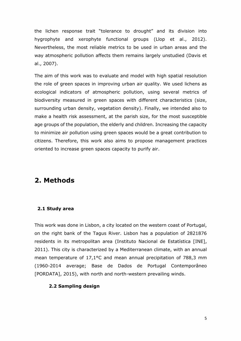
Figure 3. Boxplots of lichen diversity metrics evaluated in Lisbon green

spaces: Richness (number of species), LDVt (total lichen diversity value) and

FR (functional richness).

The number of lichen species sampled in Lisbon green spaces varied between

2 and 22 (N=42; SD=5,34) (Lichen species sampled shown in appendix I).

Total lichen diversity value, LDVt, ranged from 7 to 92 (N=42; SD=19,85)

and lichen functional richness ranged from 1 to 17 functional groups (N=42;

SD=4,14 (Figure 3). These results show the considerable range of lichens

species richness in Lisbon, from almost inexistent, to relatively rich sites.

Descriptive statistics of lichen diversity metrics can be seen in figure 3.

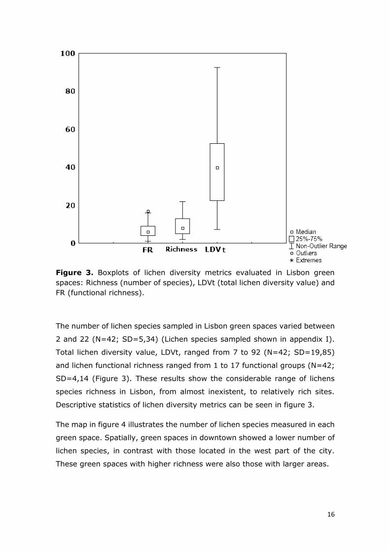
The map in figure 4 illustrates the number of lichen species measured in each

green space. Spatially, green spaces in downtown showed a lower number of

lichen species, in contrast with those located in the west part of the city.

These green spaces with higher richness were also those with larger areas.

17

Figure 4. Land-use map of Lisbon with green spaces colored in green.

Colored circles represent lichen species richness in sampling sites, ranging

from the lowest in red, to the highest in blue.

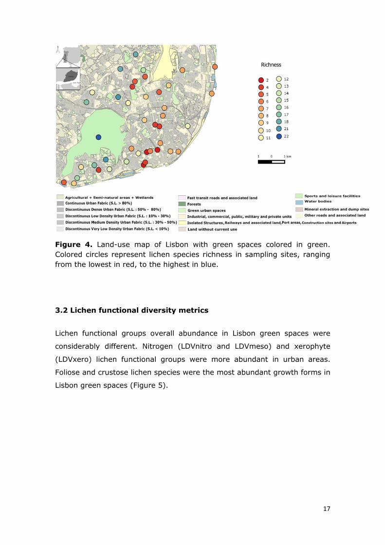
3.2 Lichen functional diversity metrics

Lichen functional groups overall abundance in Lisbon green spaces were

considerably different. Nitrogen (LDVnitro and LDVmeso) and xerophyte

(LDVxero) lichen functional groups were more abundant in urban areas.

Foliose and crustose lichen species were the most abundant growth forms in

Lisbon green spaces (Figure 5).

18

Figure 5. Boxplots of the lichen diveristy value (LDV) of each functional

group considered: LDVHygro (hygrophytic); LDVmesohygro

(mesohygrophytic); LDVxero (xerophytic); LDVnitro (nitrophytic); LDVmeso

(mesotrophic); LDVoligo (oligotrophic); LDVcru (crustose); LDVfoln (foliose

narrow); LDVfolb (foliose broad); LDVfrut (fruticose); LDVsq (squamulose),

LDVlepr (leprose).

3.3 Explaining biodiversity patterns

Individual spearman correlations were calculated to determine which factors

underlie lichen diversity patterns previously observed. Table 3 shows the

most significant correlations between environmental variables and lichen

biodiversity metrics.

The best biodiversity metrics (i.e. the highest and most significant ones) were

based in measures of total lichen diversity, such as lichen species richness

and LDVt (Table 3). Within functional diversity, functional richness (FR)

showed the highest correlation coefficient with the environmental variables.

The tolerant lichen functional groups in terms of eutrophication or water

19

requirements, nitrophytic and xerophytic, did not significantly correlate with

green spaces area, NDVIb or atmospheric NO2 concentration. Conversely, the

sensitive oligotrophic species and the foliose broad-lobed species were

significantly correlated with green spaces area and NDVIb. Crustose lichens

showed the best correlations with NO2 atmospheric concentration. Although

many metrics responded to the environmental variables, following the

parsimony principle, the higher and simple associations were considered.

Thus, only richness, LDVt and FR were chosen for further analyses. Biplots of

the selected lichen diversity metrics Richness, LDVt and FR against the most

correlated environmental variables (NO2, Area and NDVIb) are shown in

figures 6, 7 and 8.

The environmental variables showed to be significantly correlated with

several lichen biodiversity metrics (Table 3). Spearman correlations with the

remaining environmental variables are shown in appendix IV. Slope, potential

solar radiation (PSR) and distance to the coast (Dist) were not significantly

correlated with lichen biodiversity metrics (appendix IV). Conversely, altitude

was positively associated with most lichen biodiversity metrics. Tree diameter

at breast height (DBH) was negatively correlated with almost all metrics. The

area of green spaces (Arealog) and the classes of NO2 concentrations (NO2)

showed to be highly associated with the biodiversity metrics, but the area

positively whereas NO2 classes association was negative. Both NDVI inside

and in the surrounding buffer and NDVI in the centroid of the green space

(NDVIb and NDVIc, respectively) were significantly correlated with lichen

biodiversity metrics. However, since NDVIb showed the most significant

correlations and was highly correlated with NDVIc, further analyses

considered only the NDVIb. Several buffer distances (50, 100 and 200

meters) around green spaces were tested to assess the effect of urban

density. The 50 meters buffers (U50) showed the best correlation (100 and

200 meters buffer data shown in the appendix IV). From these set of

variables, the best ones were considered for model construction: Alt, Arealog,

NDVIb, NO2 and U50 (Table 3).

20

Table 3. Spearman correlation coefficients between environmental variables

and lichen biodiversity metrics. Environmental variables: Alt (altitude),

Arealog (green space logarithmized area), U50 (urban density in 50 m buffer

surrounding the green space), NO2 (NO2 atmospheric concentration) and

NDVIb (NDVI in the green space and the 100m surrounding buffer). Lichen

biodiversity metrics: Richness (species richness), FR (functional richness),

LDVHygro (hygrophytic), LDVmesohygro (mesohygrophytic), LDVxero

(xerophytic), LDVnitro (nitrophytic), LDVmeso (mesotrophic); LDVoligo

(oligotrophic); LDVcru (crustose); LDVfoln (foliose narrow), LDVfolb (foliose

broad), LDVfrut (fruticose), LDVsq (squamulose), LDVlepr (leprose).

Significant correlations are marked with an *: * = p<0,05; ** = at p<0,01;

*** = p<0, 001. N = 42.

Alt Arealog U50 NDVIb NO2

Richness 0,454

** 0,702 ***

-0,366

0,778 ***

-0,498 ***

FR

0,427

**

0,671 ***

-0,418

0,758 ***

-0,511 ***

LDVt

0,454

**

0,528

***

-0,584

0,701

***

-0,529

***

LDVnit 0,051 0,005 -0,406 0,143 -0,272

LDVmes 0,468

** 0,557 ***

-0,599 0,716 ***

-0,501 ***

LDVolig 0,443

** 0,592 ***

-0,372 0,740 ***

-0,397

LDVHygr 0,499 ***

0,482 **

-0,382 0,558 ***

-0,464

LDVmesh 0,427

** 0,641

** -0,290

0,681 ***

-0,230

LDVxer -0,026 -0,007 -0,401 0,076 -0,209

LDVcrust 0,344

* 0,372

* -0,632

0,552 ***

-0,530 ***

LDVfoln 0,077 -0,039 -0,414 0,110 -0,245

LDVfolbr 0,467

** 0,754 ***

-0,300 0,773 ***

-0,175

LDVfrut 0,256 0,416

** -0,051

0,409 **

-0,277

LDVsq 0,214 0,178 -0,152 0,233 -0,311

LDVlepr 0,422

** 0,433

** -0,172

0,492 **

-0,245

21

Figure 6. Selected lichen diversity metrics plotted with NDVIb (NDVI of the

green spaces and the 100 meters buffer). Lichen diversity metrics: species richness (Richness), total lichen diversity value (LDVt) and functional richness

(FR). The line was included to represent the shape of the relationship and was done using a smoothing function (Distance Weight Least Squares) with a 0.65 stiffness.

22

Figure 7. Selected lichen diversity metrics plotted with green spaces area

(Area log, logarithmized area). Lichen diversity metrics: species richness

(Richness), total lichen diversity value (LDVt) and functional richness (FR).

The line was included to represent the shape of the relationship and was done

using a smoothing function (Distance Weight Least Squares) with 0.65

stiffness.

23

Figure 8. Selected lichen diversity metrics plotted with NO2 atmospheric

concentration (μg/m3; NO2 concentration values are grouped in class 1: >35

μg/m3; class 2: 30 - 35 μg/m3; class 3: 20 - 30 μg/m3; class 4: < 20 μg/m3).

Lichen diversity metrics: species richness (Richness), total lichen diversity

value (LDVt) and functional richness (FR). The line was included to represent

the shape of the relationship and was done using a smoothing function

(Distance Weight Least Squares) with a 0.65 stiffness.

3.4 Lichens richness model for green spaces

Several models were built for the estimation of lichens richness in urban

green spaces using the set of previously selected environmental variables and

24

lichen diversity metrics (section 3.2 Lichen functional diversity metrics), using

GLM (Generalized linear models). The identify link was used because all

relationships approached a linear shape. Models with green space area as

variable could not be satisfactorily fitted using these model specifications, due

one sampling site that had a much higher area than the others (site

Monsanto). Thus, this site was excluded from the models. Without it, the

relationships with area were linear. Lichen diversity value and species

richness air quality models showed similar results. For this reason, only the

models for species richness are shown. After running all possible

combinations, only the five models with higher AICs were selected and are

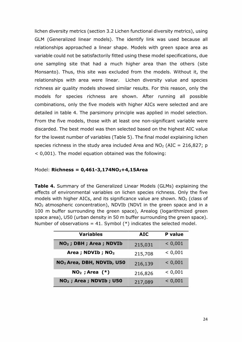
detailed in table 4. The parsimony principle was applied in model selection.

From the five models, those with at least one non-significant variable were

discarded. The best model was then selected based on the highest AIC value

for the lowest number of variables (Table 5). The final model explaining lichen

species richness in the study area included Area and NO2 (AIC = 216,827; p

< 0,001). The model equation obtained was the following:

Model: Richness = 0,461-3,174NO2+4,15Area

Table 4. Summary of the Generalized Linear Models (GLMs) explaining the

effects of environmental variables on lichen species richness. Only the five

models with higher AICs, and its significance value are shown. NO2 (class of

NO2 atmospheric concentration), NDVIb (NDVI in the green space and in a

100 m buffer surrounding the green space), Arealog (logarithmized green

space area), U50 (urban density in 50 m buffer surrounding the green space).

Number of observations = 41. Symbol (*) indicates the selected model.

Variables AIC P value

NO2 ; DBH ; Area ; NDVIb 215,031 < 0,001

Area ; NDVIb ; NO2 215,708 < 0,001

NO2 Area, DBH, NDVIb, U50 216,139 < 0,001

NO2 ; Area (*) 216,826 < 0,001

NO2 ; Area ; NDVIb ; U50 217,089 < 0,001

25

Table 5. Regression results obtained by a generalized linear model explaining

lichen species richness using green spaces area and class of NO2 atmospheric

concentration. The values given are the predictor’s estimates. Standard

errors are shown in parenthesis. Predictor variables: NO2 (Classes of NO2

concentrations (μg/m3)); Arealog (green spaces logarithmized area (m2)).

Effects Model

Intercept 0,461

(2,675)

NO2 -3,174

***

(0,642)

Arealog 4,15 ***

(0,592)

No. of observations 42

The effect of interactions between variables was tested and the results

showed that there was no significant interaction (data not shown). Results of

cross validation performed for the model are shown in table 6. A tendency for

underestimating maximum values was observed, but the average and median

predicted values fitted well the observed ones. Plotting the observed versus

predicted values showed a small tendency for overestimation of the number

of species in sites with less species (Figure 9).

Table 6. Statistics for the observed and predicted values obtained by cross-

validation of a generalized linear model explaining lichen species richness

using green spaces area and class of NO2 atmospheric concentration. Error

26

average was determined calculating the modulus of the difference between

the observed and the predicted values.

Predicted

values

Observed

values

Average 9,171 9,195

Coefficient of Variation 45,80 57,146

Max 16 21

Min 1 2

Median 9 8

Standard Deviation 4,201 5,255

Error average 2,683

Figure 9. Predicted values of a generalized linear model explaining lichen

species richness using green spaces area and class of NO2 plotted with the

observed values. This was performed on 10 subsamples of approximately

10% randomly chosen values. Regression bands with 95% confidence level

are shown.

27

3.5 Applying the lichens species richness model to other green

spaces

The model developed previously was used to estimate lichen species richness

for other Lisbon green spaces. Results show that lichen species richness is

lower in the center-south of the city, as already seen from sampled lichen

diversity (figure 10).

Figure 10. Land-use map of Lisbon. Colored circles represent estimated

lichen species richness ranging from low (red) to high (blue) for each green

space of the city.

28

Figure 11. Land-use map of Lisbon. Colored circles represent model

residuals.

As estimated values were slightly biased, residuals of the estimates of lichen

species richness were plotted to understand its spatial distribution. The

analysis of the residuals map shows that the areas immediately south and SE

of the airport lichen diversity values are overestimated when compared to the

observed values. The center of Lisbon corresponds to the area where the

model more accurately reflects the observed values (Figure 11).

29

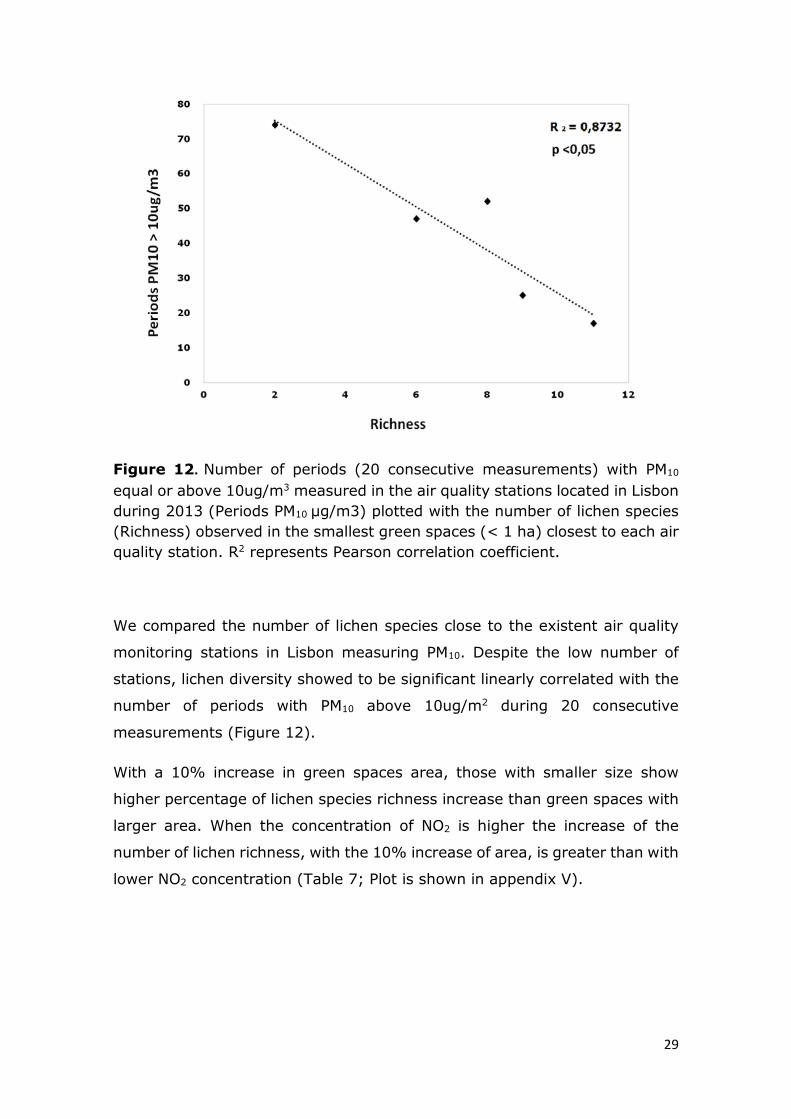
Figure 12. Number of periods (20 consecutive measurements) with PM10

equal or above 10ug/m3 measured in the air quality stations located in Lisbon

during 2013 (Periods PM10 μg/m3) plotted with the number of lichen species

(Richness) observed in the smallest green spaces (< 1 ha) closest to each air

quality station. R2 represents Pearson correlation coefficient.

We compared the number of lichen species close to the existent air quality

monitoring stations in Lisbon measuring PM10. Despite the low number of

stations, lichen diversity showed to be significant linearly correlated with the

number of periods with PM10 above 10ug/m2 during 20 consecutive

measurements (Figure 12).

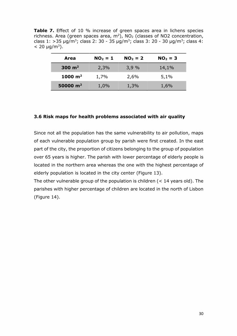
With a 10% increase in green spaces area, those with smaller size show

higher percentage of lichen species richness increase than green spaces with

larger area. When the concentration of NO2 is higher the increase of the

number of lichen richness, with the 10% increase of area, is greater than with

lower NO2 concentration (Table 7; Plot is shown in appendix V).

30

Table 7. Effect of 10 % increase of green spaces area in lichens species

richness. Area (green spaces area, m2), NO2 (classes of NO2 concentration, class 1: >35 μg/m3; class 2: 30 - 35 μg/m3; class 3: 20 - 30 μg/m3; class 4:

< 20 μg/m3).

Area NO2 = 1 NO2 = 2 NO2 = 3

300 m2 2,3% 3,9 % 14,1%

1000 m2 1,7% 2,6% 5,1%

50000 m2 1,0% 1,3% 1,6%

3.6 Risk maps for health problems associated with air quality

Since not all the population has the same vulnerability to air pollution, maps

of each vulnerable population group by parish were first created. In the east

part of the city, the proportion of citizens belonging to the group of population

over 65 years is higher. The parish with lower percentage of elderly people is

located in the northern area whereas the one with the highest percentage of

elderly population is located in the city center (Figure 13).

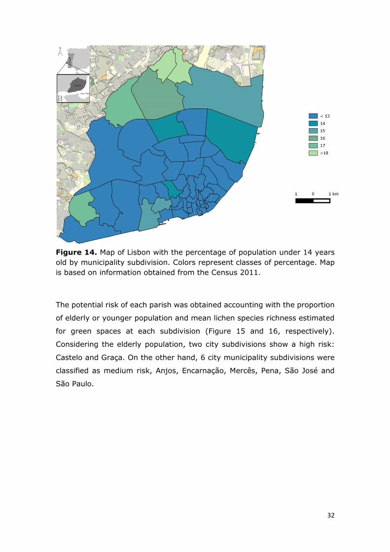
The other vulnerable group of the population is children (< 14 years old). The

parishes with higher percentage of children are located in the north of Lisbon

(Figure 14).

31

Figure 13. Map of Lisbon showing the percentage of population over 65 years old by municipality subdivision (municipality subdivision). Colors represent

classes of percentage. Map is based on information obtained from the Census 2011.

32

Figure 14. Map of Lisbon with the percentage of population under 14 years

old by municipality subdivision. Colors represent classes of percentage. Map

is based on information obtained from the Census 2011.

The potential risk of each parish was obtained accounting with the proportion

of elderly or younger population and mean lichen species richness estimated

for green spaces at each subdivision (Figure 15 and 16, respectively).

Considering the elderly population, two city subdivisions show a high risk:

Castelo and Graça. On the other hand, 6 city municipality subdivisions were

classified as medium risk, Anjos, Encarnação, Mercês, Pena, São José and

São Paulo.

33

Figure 15. Average lichen species richness estimated for Lisbon at the parish

level (Richness) plotted with the percentage of elderly people (>65 years old)

in the same subdivision (% elderly). Letter L represents low risk parishes, M

represents medium risk and H represents high risk parishes.

Figure 16. Average species richness estimated for Lisbon at the parish level

(Richness) plotted with the percentage of younger population (0-14 years

34

old) in the same municipality subdivision (% children). Letter L represents

low risk parishes, M represents medium risk and H represents high risk

parishes.

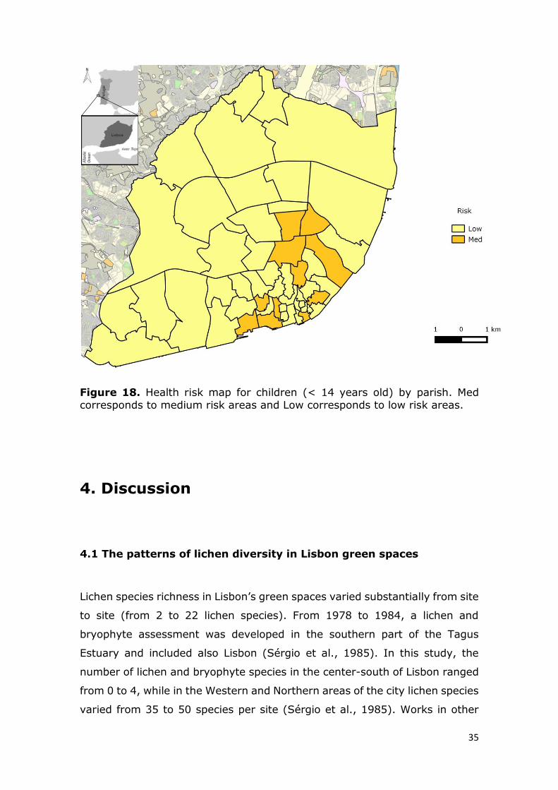
The health risk maps obtained for Lisbon elderly and younger population are

shown in figures 17 and 18, respectively. For both vulnerable population

groups, the highest risk is always in the center-south of the city.

Figure 17. Health risk map for elderly people (> 65 years old) by parish. High corresponds to a high risk areas, Med corresponds to medium risk areas and Low corresponds to low risk areas.

35

Figure 18. Health risk map for children (< 14 years old) by parish. Med

corresponds to medium risk areas and Low corresponds to low risk areas.

4. Discussion

4.1 The patterns of lichen diversity in Lisbon green spaces

Lichen species richness in Lisbon’s green spaces varied substantially from site

to site (from 2 to 22 lichen species). From 1978 to 1984, a lichen and

bryophyte assessment was developed in the southern part of the Tagus

Estuary and included also Lisbon (Sérgio et al., 1985). In this study, the

number of lichen and bryophyte species in the center-south of Lisbon ranged

from 0 to 4, while in the Western and Northern areas of the city lichen species

varied from 35 to 50 species per site (Sérgio et al., 1985). Works in other

36

European cities showed similar current species richness ranges in urban

areas, but with a more marked trend of increase in species richness over

time. In London, a work performed in 2004 showed that the number of lichen

species per site varied from 8 to 25 (Davies et al., 2007), whereas in the 70’s

the number of lichen species in that city varied only between 0 and 7 (Davies

et al., 2007). Also in the Finish city of Tampere the number of lichen species

increased from a range of 0 to 7 in 1980, to 3 to 14 species in 2000 (Ranta,

2001). Like species richness, also the pattern of LDVt found in Lisbon green

spaces varied among sites, ranging from 7,25 to 83,75. This pattern of

variation is also similar to that found in Central London (8,6 - 76,9 ; Larsen

et al., 2006) or in a small Portuguese city (c.15 to 60; Llop et al., 2012).

The range of air quality we observed in Lisbon is comparable to that of London

(a larger city) and to a smaller city in Finland (Davies et al., 2007; Ranta,

2001; Larsen et al., 2006) and Sines (Llop et al., 2012). This suggests that

these patterns of considerable variation of lichen species richness and LDVt

in urban areas are generalized, and that the pattern is not exclusive to large

cities. These cities’ heterogeneity in terms of air pollution highlights the need

for maps with high spatial resolution for informed management decisions can

be made. The temporal trends of air pollution in cities suggest the importance

of the background air pollution component, in addition to the important role

of current local sources of pollution. A substantial increase in the number of

lichen species was observed from the 70’s or 80’s to the present time in

European cities (Davies et al., 2007; Ranta, 2001). In Lisbon, this air quality

improvement was not so apparent. Our results from the center-south parts

of Lisbon suggest a similar air quality to that assessed by Sérgio et al. (1985)

in the 70’s. On the other hand, in the 70’s the air quality seemed to be better

in Western and Northern areas than in present day, as shown by the higher

number of lichens and bryophytes observed then. These temporal patterns

can be explained by several factors. Since the 70’s the city expanded to some

areas that had quite reasonable air quality, areas that were probably closer

to green spaces in the past. The worsening of conditions observed by us in

2015 may probably be due to land use change, resulting from the conversion

of green spaces to constructed areas. Moreover, the higher number of lichens

and bryophytes observed in the 70’s might not be so directly comparable to

37

that sampled by us. Numbers might be biased: 1) by the fact that they

account with both groups together; 2) the sampling methodology was

different back then and included the visualization of the whole tree trunk and

branches, in opposition to the method used by us that inspects only a small

area at breast height. In addition to these factors, Portugal was not so highly

industrialized as were most European countries in the 70’s and 80’s, nor did

the levels of charcoal combustion for house heating in Portugal closely

resembled other European regions. The industrialization started later in

Portugal and with cleaner technologies. This could have probably influenced

Lisbon air quality, which had probably less sulphur dioxide and particles than

most other European capitals during the 70’s and 80’s. In fact, the maximum

values of diversity in other European cities in the 70’s were considerably lower

than that observed in Lisbon (Davies et al., 2007; Ranta, 2001; Sergio et al.,

1985). Also, the increase in the number of vehicles from the 70’s to present

day occurred simultaneously with less emissions per vehicle due to cleaner

technologies, justifying the apparent maintenance of the same ranges of air

quality in Lisbon.

In this work Xerophytic and Nitrophytic lichens were the most abundant

functional groups, together with foliose narrow and crustose growth forms.

Also in London a higher abundance of nitrophytic lichens was reported (Davies

et al., 2007). These results can be supported by the fact that cities are

associated with high nitrogen concentrations both NOx and NH3 (Svirejeva-

Hopkins et al. 2011). Moreover, due to the urban heat island effect the

temperature is higher and the relative humidity is lower, particularly in the

center of the city (Oke, 1987). Fruticose lichens were the least abundant. This

is probably related to their sensitivity to air pollution, since this functional

group is regarded as the most sensitive to air pollution due to its large surface

area of exposure to atmosphere (Awasthi 2000).

The oligotrophic lichen functional group was the most correlated with the area

of green spaces and the NDVIb. At the same time, oligotrophic species were

negatively associated with anthropogenic pressure measure here by NO2

atmospheric concentration which is used here as a surrogate traffic intensity

and thus of air pollution in cities caused by traffic (Ito et al., 2007; Moldanová

et. al, 2011), because it is usually one of the easiest to measure and map at

38

a high spatial resolution, in opposition to particles or SO2, for instance. In our

case, NO2 atmospheric concentration was used because it was the only

pollutant available with a relatively good spatial resolution. This pollutant is

known to have high deleterious effects on lichens under controlled conditions

at concentrations two orders of magnitude higher (c. 6 mg/m3) (Nash III,

1976) than those found currently in Lisbon (<4 µg/m3). The negative relation

found between NO2 concentration and the oligotrophic lichens suggests that

this relationship is in fact reflecting the effects of other pollutants usually

emitted together with NO2 which are known to affect lichens for

concentrations closer to the ones observed in urban areas such as SO2 and

particles (Showman, 1972). A recent work exposed lichens to diesel exhaust

under controlled conditions and showed that lichens were affected by the

mixture of pollutants present although they were not able to separate the

individual pollutants effects (Langmann et al., 2014). A work from Pinho and

co-workers (2008) showed the high sensitivity of oligotrophic lichen species

to general increased levels of pollutants in a multipollutant area. This group

sensitivity was also demonstrated in small cities, as their abundance was

lower in areas near roads, when compared to parks and residential areas

(Llop et al., 2012).

Lichen species richness was the biodiversity metrics that best performed in

response to the environmental variables and, thus, the one selected to be

used as a surrogate of air quality and for model construction. This metric is a

simple and very intuitive measure that can be easily communicated for

general public and stakeholders as an air quality measure. Other metrics

including the ones that have in account cover of species (LDVt) and functional

richness (FR) gave similar results but we decided to use a simple and intuitive

biodiversity metrics the number of lichen species.

4.2 Factors affecting air quality in green spaces

Most lichen diversity metrics tested showed correlations with the

environmental factors. In general, an increase in the green space area lead

39

to an increase in species richness, LDVt and the LDV of functional groups,

except for the most tolerant functional groups in terms of water requirements

and eutrophication (xerophytic and nitrophytic). Although we were able to

observe some changes in the abundance of lichen communities and in lichen

functional diversity, those were not as clear as the marked decline in the

number of lichen species. In cities smaller than Lisbon, functional groups

responded better than total diversity to gradients of environmental change

from rural to urban areas induced by different land-use in urban areas (Llop

et al., 2012; Munzi et al., 2014). In both cases moving closer to cities or

closer to more disturbed sites had no strong effect in the number of lichen

species, but induced changes in the community, with the most sensitive

species being replaced by the tolerant ones (Munzi et al., 2014; Llop et al.,

2012). The authors suggested the shift to a more nytrophytic community to

be an effect of alkaline dust particles and/or atmospheric NH3 emitted by

traffic (Llop et al., 2012). On the other hand, the observed shifts to xerophytic

dominated communities were suggestive of a heat island effect (Munzi et al.,

2014). In our work we did not observe clear shifts in the communities, neither

in relation to water requirements, nor in relation to eutrophication. This lack

of clear communities’ shifts together with the dramatic decrease in species

richness are a clear indication that in Lisbon air pollution levels are still high

enough to have a deleterious effects on the overall lichen community.

Moreover, the lack of clear community shifts related to water requirements,

suggests that the pollution driver still plays a more important role in the city

than the heat island effect, due to its large size and traffic intensity. Thus,

the main factor determining the distribution of lichen species in Lisbon is the

level of air quality.

As expected lichens species richness decreased in areas with higher PM10

concentrations, showing a high association between lichens species richness

and air pollution. Our results suggest that PM10 concentrations affect lichens

richness, which is supported by other works (Langmann et al., 2014).

Therefore, lichens species richness is used as a sorrugate for air quality of

green spaces.

We found that the most important factors explaining air quality in Lisbon

green spaces were the size of the green space (Area), the tree density

40

(NDVIb) and the traffic intensity (concentration of NO2). Taking into

consideration that we considered lichen species richness as a surrogate of air

quality, thus an increase in lichen richness can be associated to an

improvement in air quality. NDVIb was the most significant factor in relation

with the lichen metrics, followed by Area and NO2 respectively. Zupancic and

co-workers’ review (2015) suggested that vegetation density is the main

responsible for the ecosystem service air purification in urban forests. Our

results also suggest that air purification increases with green space area. In

fact, a previous work showed that the size of the green space is important to

reduce the penetration of air pollutants (Ali, 2013). Moreover, some

pollutants, such as particulate material have short deposition distances

(<500m). This along with tree leaves roughness make it more difficult to

particles to reach the central area of a green space (Gheorghe & Ion, 2011).

Thus, our work reinforces from an ecological indicator perspective the

important role that size and tree density of cities’ green spaces have in

providing the service air purification. This represents an innovation of this

work, in the sense that it tackles simultaneously a large range of green space

sizes together with ecological indicators evaluation.

Other factors were also found to be associated with lichen species richness.

However, they were likely associated to the green space area, tree density or

the concentration of NO2, providing no extra explanation for understanding

the patterns of lichen species richness patterns. The type of matrix around

each green space was relevant, with the proportion of area covered by urban

density around each green space negatively influencing the air quality in its

center. Similar results were also observed in the smaller city of Almada

showing that the urban density matters for the effects of the urban heat island

effect (Munzi et al., 2014). The results also show a significant positive

association of air quality with increasing altitude. Valleys channel air flow and

frequently "trap" polluted air originating high pollutant concentrations at

lower altitudes (Falke & Schichtel, 2000). Lisbon city center is associated with

a valley (Alcoforado, 2009) and, as seen in our work, has higher air pollution

(seen with the sorrugate NO2 concentration).

41

Environmental variables more related to microclimatic conditions, such as

slope, distance from the coastline and PSR, did not show a significant

association with green spaces air quality. This supports our conclusion that

air quality is the main factor affecting lichen metrics, rather than other factors

related with microclimate. These factors can influence lichens (e.g. by

favoring hygrophytic lichens in areas more protected from the sun, with lower

PSR values, Pinho, 2010), but this is only visible when atmospheric pollution

is found at lower levels than those found in Lisbon.

Interestingly, some green spaces revealed large deviations between the

observed and predicted values. These green spaces are mostly located near

the airport. The variable that we used as surrogate of vehicle traffic is NO2

modeled for the city of Lisbon in only 4 classes and for 2001. Some changes

might have occurred during this period namely the substantial increase in air

traffic close to the airport during the last years. Further work is necessary

here to evaluate the real impact that the airport traffic has on the surrounding

area.

4.3 The role of Lisbon gardens in air purification

Green spaces in the city clearly showed to provide air purification service but

how much can we rely on them for improving air quality? In the same region

with the same background pollution level, a green space area increase of 10%

has a much higher effect in small green space located in polluted areas than

in larger ones located in cleaner areas of the city. For instance, a green space

with 300 m2 of area has a 14,1% increase air purification service while one

with 50000 m2 has only a 1,3% increment, in a NO2 concentration of 20 –

30μg/m3 (class 3). Because lichen species richness seem to vary linearly with

one of the main components of urban air pollution, which are dust particles,

we can assume that air quality also improved linearly with the increase in the

number of lichen species.

It is important to note that the relationship between the area of a green space

and species richness is not linear, but rather logarithmic (note that area was

log prior to modeling, thus resulting in a linear relationship for the model).

42

As a consequence, the establishment of small gardens, or the increase of area

in small ones, will result in a large gain of air quality improvement, when

compared to building large gardens or increasing those already large. This

effect would be especially relevant in very dense urban areas, where the

existing green spaces are few and small and no space is available for larger

green spaces. One important result of the model was to show that extremely

large green spaces (Monsanto, ~1000ha) do not hold many more species

than the very large ones (e.x. Parque Bensaude ~22ha). In fact both

sites present a similar number of species (c. 20), which likely corresponds to

the background maximum number of species per site in the region. Thus,

increasing the area of a green space above 10ha is probably not going to

cause any further increase in local air quality.

As expected, in the city center-south air quality of green spaces is low there

are high density of urban areas (with buildings occupying about 50% of the

total floor area) and green spaces are conspicuously absent (Alcoforado et

al., 2009).

4.4 Air quality in Lisbon: focusing on risk areas for humans

In this work a health risk map was built for Lisbon parishes. The city center-

south is where air quality is worse and, thus, where the resident population

is at higher risk. In this area, air pollution in green spaces is worse and the

percentage of elderly people is higher, thus resulting in a higher risk area for

this population group. The younger population lives mostly in parishes further

away from the city center, thus with better air quality, which results in a lower

risk for this susceptible group.

Considering the lack of green spaces with larger areas in the center of the

city and the percentage of elderly people in some parishes, this is an area

that requires special attention. A mitigation measure could be the

construction or increase of small green spaces, which would have a large

impact in this area as previously explained. If not possible, increasing tree

density in the existing green spaces should be considered. As air quality in

43

an urban green spaces improved with increasing vegetation density, the

readjustment of the existing green spaces by planting additional trees, can

be an alternative. Green roofs, green walls and increasing the number of trees

and shrubs on road sides are other options that can be implemented.

As expected air pollution driver by traffic intensity (e.g. seen using NO2 or

particles as surrogates) determined air quality of urban green spaces (seen

using lichen species richness as a surrogate). Given the relationship of e.g.

particulate matter with health, any direct measures to decrease air pollution

would result in a direct gain in air quality, and should be considered together

with the precious suggested measures. Close car traffic on roads, decrease

traffic in the city center by restricting non-electric cars circulation in some

streets and reducing the traffic by changing roads with two ways by just one

are examples of these direct measures.

5. Final remarks

This work suggests that atmospheric pollution is the preponderating factor

affecting lichen diversity in Lisbon. As a consequence, total diversity metrics

like species richness responded better to the predominant environmental

factors than functional diversity, thus being the best ecological indicator of

air quality for Lisbon green spaces. Further work should be done to evaluate

the impact of atmospheric pollution due to the Lisbon airport.

For the first time, we were able to map air quality in more than 100 green

spaces in Lisbon. The map was based on a model of air quality evaluated

through an ecological indicator, using Area and NO2 concentration as the

explaining variables. This represents also an innovation, in the sense that it

tackles simultaneously a large range of green space sizes together with

ecological indicators evaluation, something that is innovative. The best

variables explaining air pollution reduction effect of urban green spaces were

tree density, green space area and the NO2 concentration. These results

44

highlight the importance of green spaces for providing the air purification

service. The model built uses a small number of variables, an advantage that

makes it easier to be applied.

A risk map was constructed concealing susceptible population distribution and

green spaces air quality. The higher risk areas are located in the city centre,

were elderly population is also more dense. This risk map can be applied by

decision and policy makers to plane future city interventions. Considering the

difficulties in increasing the number of green spaces or their size in the city

center, due to the high urban density, is suggested to increase tree density.

Green roofs and green walls are also a good measure to go beyond these

problems.

45

References

Alcoforado, M. J., Andrade, H., Lopes A. & Vasconcelos, J. (2009) Application

of climatic guidelines to urban planning: The example of Lisbon (Portugal).

Landscape and Urban Planning, 90, 56–65.

Ali, M. (2013) The contribution of urban green spaces in the regulation of the

microclimate and the improvement of the air quality in cities. Asian Journal

of Current Engineering and Maths, 190 - 195.

Asta, J., Erhardt, W., Ferretti, M., Fornasier, F., Kirschbaum, U., Nimis, P. L.,

Purvis, O., Pirintsos, S., Scheidegger, C., van Haluwyn, C. & Wirth, V. (2002)

Mapping lichen diversity as an indicator of environmental quality. In P.L.

Nimis, C. Scheidegger & P.A. Wolseley (Ed.), Monitoring with Lichens –

Monitoring Lichens (pp. 273-279). Netherlands: Kluwer Academic Publisher.

Berto, R. (2005) Exposure to restorative environments helps restore

attentional capacity. Journal of Environmental Psychology, 25, 249–259.

Bolund, P. & Hunhammar, S. (1999) Ecosystem services in urban areas.

Ecological Economics, 29, 293–301.

Bowler, D., Buyung-Ali, L., Knight, T., & Pullin, A. S. (2010) How effective is

‘greening ‘of urban areas in reducing human exposure to ground level ozone

concentrations, UV exposure and the ‘urban heat island effect’. Environmental

Evidence: www. Environmental evidence. org/SR41. Html

Branquinho, C. (2001) Lichens. In M.N.V. Prasad (Ed.) Metals in the

Environment: Analysis by Biodiversity. (pp. 117-158.) New York: Marcel

Dekker.

Caro, T. (2010) Conservation by proxy. Indicator, umbrella, keystone,

flagship, and other surrogate species. Washington D.C. : Island Press.

Cavanagh, J. E., J.-A.E., Zawar-Reza, P., & Wilson, J. G. (2009) Spatial

attenuation of ambient particulate matter air pollution within an urbanised

native forest patch. Urban Forestry & Urban Greening, 8(1), 21-30.

46

Chen, B. & Kan, H. (2008) Air pollution and population health: a global

challenge. Environmental Health and Preventive Medicine, 13, 94–101.

Costanza, R., d’Arge, R., de Groot, R., Farber, S., Grasso, M., Hannon, B.,

Limburg, K., Naeem, S., O’Neill, R., Paruelo, J., Raskin, R., Sutton, P. & Van

den Belt, M. (1997) The value of the world’s ecosystem services and natural

capital. Nature, 387 (15), 253–260.

Dale, V. H. & Beyeler S. C. (2001) Challenges in the development and use of

ecological indicators. Ecological Indicators, (1), 3–10.

Davies, L., Bates, J. W., Bell, J. N. B., James, P. & Purvis, O. W. (2007)

Diversity and sensitivity of epiphytes to oxides of nitrogen in London.

Environmental Pollution, 146(2), 299-310.

Davies, Z. G., Edmondson, J. L., Heinemeyer, A., Leake, J. R. & Gaston, K. J.

(2011) Mapping an urban ecosystem service: quantifying above-ground

carbon storage at a city-wide scale. Journal of Applied Ecology, 48, 1125–

1134.

Diaz, S. & Cabido, M. (2001) Vive la difference: Plant functional diversity

matters to ecosystem processes. Trends in Ecology and Evolution, 16, 646 -

655.

European Environmental Agency (2014) Air quality report in Europe – 2014

Report, 80.

Fenger, J. (2009) Air pollution in the last 50 years – From local to global.

Atmospheric Environment, 43 (1), 13–22.

Gheorghe, I., & Ion, B. (2011) The Effects of Air Pollutants on Vegetation and

the Role of Vegetation in Reducing Atmospheric Pollution. In Earth and

Planetary Sciences - Oceanography and Atmospheric Sciences. InTech.

Giordani, P., Brunialti, G. & Alleteo, D. (2002) Effects of atmospheric

pollution on lichen biodiversity (LB) in a Mediterranean region (Liguria,

northwest Italy). Environmental Pollution, 118, 53–64.

47

Gitay, H. & Noble, I. R. (1997) What are functional types and why should we

seek them? In: Smith, T. M. Shugart, H. H., Woodward, F. I. (Ed.) Plant

Functional Types. University Press, Cambridge, 3-19.

Givoni, B. (1991) Impact of planted areas on urban environmental quality: a

review. Atmospheric Environment Part B Urban Atmosphere, 25(3), 289–299.

Hale, M. E (1983) The biology of lichens. London: Mason Edward Arnold Ltd.

Hauck, M. (2010) Ammonium and nitrate tolerance in lichens. Environmental

Pollution, 158, 1127–1133.

Honegger, R. (1991) Functional aspects of the lichen symbiosis. Annual

Review of Plant Physiology and Molecular Biology 42, 553 - 578.

Ito, K., George, D. T. & Silverman, R. A. (2007) Characterization of PM2.5,

gaseous pollutants, and meteorological interactions in the context of time-

series health effects models. Journal of Exposure Science and Environmental

Epidemiology, 17, S45–S60.

Jansson, M. (2014) Green space in compact cities: the benefits and values of

urban ecosystem services in planning. Nordic Journal of Architectural

Research, 26 (2), 139-160.

Lakes, T. & Hyun-Ok, K. (2012) The urban environmental indicator “Biotope

Area Ratio”— An enhanced approach to assess and manage the urban

ecosystem services using high resolution remote-sensing. Ecological

indicators, 13, 93-103.

Langmann, U., Madl, P., Türk, R., Hofmann, W. & Brunauer, G. (2014)

Sensitivity of Lichens to Diesel Exhaust under Laboratory Conditions. Journal

of Environmental Protection, 5, 1331-1341.

Larsen, R.S., Bell, J.N.B. , James, P.W., Chimonides , P.J., Rumsey, F.J.,

Tremper , A., Purvis, O.W. (2007) Lichen and bryophyte distribution on oak

in London in relation to air pollution and bark acidity. Environmental Pollution,

146, 332 and 340.

Lindenmayer, D., Piersona, J., Bartona, P., Begerb, M., Branquinho, C.,

Calhound, A., Caroe, T., Greigf, H., Grossg, J., Heinoh, J., Hunterd, M.,

Lanea, P., Longoi, C., Martinj, K., McDowellk, W. H., Mellinl, C., Salom, H.,

48

Tullocha, A. & Westgatea, M. (2015) A New framework for selecting

environmental surrogates. Science of the Total Environment. In press.

Llop, E., Pinho, P., Matos, P., Pereira, M. J. & Branquinho, C. (2012) The use

of lichen functional groups as indicators of air quality in a Mediterranean

urban environment. Ecological Indicators, 13, 215–221.

Mellin, C., Delean, S., Caley, J., Edgar, G., Meekan, M., Pitcher, R.,

Przeslawski, R.,Williams, A. & Bradshaw, C. (2011) Effectiveness of biological

surrogates for predicting patterns of marine biodiversity: a global meta-

analysis. PLoS One, 6 (6).

Mesquita, S. M. P. (2009) Modelação da distribuição espacial da qualidade do

ar em Lisboa usando sistemas de informação geográficas (master’s thesisi).

Retrieved from http://hdl.handle.net/10362/4038.

Moldanová, J., Grennfelt, P. & Jonsson, A. (2011) Nitrogen as a threat to

European air quality. In M. A. Sutton, C. M. Howard, J. W. Erisman, G. Billen,

A. Bleeker, P. Grennfelt, H. Grinsven, B. Grizzetti (Ed.) The European

Nitrogen Assessment. Cambridge: Cambridge University Press.

Munzi, S., Correia, O., Silva, P., Lopes, N., Freitas, C., Branquinho, C. &

Pinho, P. (2014) Lichens as ecological indicators in urban areas: beyond the

effects of pollutants. Journal of Applied Ecology, 51, 1750-1757.

Nimis, P.L. & Martellos, S. (2002) ITALIC—the information system on Italian

lichens. In D. K. Upreti, P.K. Divakar, V. Shukla, R. Bajpai (Ed.) Sampling and

Interpreting Lichen Diversity Data for Biomonitoring Purposes. Recent

Advances in Lichenology. Modern Methods and Aproaches in Biomonitoring

and Bioprospect, 1, 265.

Nimis, P.L. & Purvis, W.O. (2002) Monitoring lichens as indicators of pollution.

In P.L. Nimis, C. Scheidegger, P.A. Wolseley (Ed.), Monitoring with Lichens -

Monitoring Lichens (pp. 7 and 10) NATO Advanced Science Series, Kluwer.

Nimis, P.L., Ciccarelli A., Lazzarin G., Bargagli R., Benedet A. & Castello M.

(1989) I licheni come bioindicatori di inquinamento atmosferico nell'area di

Schio – Thiene – Breganze (VI). Bolletino del Museo Civico di Storia Naturale

di Verona , 16, 1–154.

49

Oke, T. R. (1987) Boundary Layer Climates. 2nd edition. London, UK:

Routledge.

Organisation for Economic Co-operation and Development (OECD) (2014)

The Cost of Air Pollution: Health Impacts of Road Transport. OECD Publishing.

Pinho, P. (2010) Temporal and spatial patterns of lichens functional groups

as ecological indicators of the local effects of global-change drivers within

Mediterranean forests (Doctoral dissertation). Retrieved from

http://hdl.handle.net/10451/2303.

Pinho, P., Bergamini, A., Carvalho, P., Branquinho, C., Stofer, S.,

Scheidegger, C. & Maguas, C. (2012) Lichen functional groups as ecological

indicators of the effects of land-use in Mediterranean ecosystems. Ecological

Indicators, 15, 36-42.

Pinho, P., Branquinho, C., Cruz, C., Tang Y. S., Dias, T., Rosa, A. P., Máguas,

C., Martins-Loução , M. A. & Sutton, M. A. (2009) Assessment of Critical

Levels of Atmospheric Ammonia for Lichen Diversity in Cork-Oak Woodland,

Portugal. In Atmospheric Ammonia (pp 109-119). Netherlands: Springer

Netherlands.

Pinho, P., Dias, T., Cruz, C., Tang, Y.S., Sutton, M., Martins-Loucao, M.A.,

Maguas, C. & Branquinho, C. (2011) Using lichen functional-diversity to

assess the effects of atmospheric ammonia in Mediterranean woodlands.

Journal of Applied Ecology, 48, 1107–1116.

Pinho, P., Llop, E., Ribeiro, M.C., Cruz, C., Soares, A., Pereira, M.J. &

Branquinho, C. (2014) Tools for determining critical levels of atmospheric

ammonia under the influence of multiple disturbances. Environmental

Pollution, 188, 88-93.

Ranta, P. (2001) Changes in urban lichen diversity after a fall in sulphur

dioxide levels in the city of Tampere, SW Finland. Annales Botanici

Fennici, 38(4), 295–304

Schleuter, D., Daufresne, M., Massol, F. & Argillier, C. (2010) A user's guide

to functional diversity indices. Ecological Monographs , 80, 469–484.

50

Selevan, S. G., Kimmel, C. A., & Mendola, P. (2000) Identifying critical

windows of exposure for children’s health. Environmental Health

Perspectives, 108 (3), 451–455.

Showman, R. E. (1972) Residual Effects of Sulfur Dioxide on the Net

Photosynthetic and Respiratory Rates of Lichen Thalli and Cultured Lichen

Symbionts. The Bryologist, 75 (3), 335-341.

Simoni, M., Baldacci, S., Maio, S., Cerrai, S., Sarno, G., & Viegi, G. (2015)

Adverse effects of outdoor pollution in the elderly. Journal of Thoracic

Disease, 7(1), 34–45.

Svensson, M. & Eliasson I. (1997) The importance of green areas for the

ventilation of the city. Naturvardsverkets rapport 4779, Stockholm.

Svirejeva-Hopkins, A., Stefan, R., Magid, J., Nardoto, G. B., Barles, S.,

Bouwman, A. F., Erzi, I., Kousoulidou, M., Howard, C. M. & Sutton, M. A.

(2011) Nitrogen flows and fate in urban landscapes. In M. A. Sutton, C. M.

Howard, J. W. Erisman, G. Billen, A. Bleeker, P. Grennfelt, H. V. Grinsven, B.

Grizzetti. (Ed.) The European Nitrogen Assessment (pp. 249-270).

Cambridge: Cambridge University Press.

Ulrich, R. S., Simons, R. F., Losito, B. D., Fiorito, E., Miles, M. A., & Zelson,

M. (1991) Stress recovery during exposure to natural and urban

environments. Journal of Environmental Psychology, 11, 201–230.

United Nations (UN) (2014). World Urbanization Prospects: The 2014

Revision, Highlights.

World Health Organization (WHO) (2014) Burden of disease from Ambient Air

Pollution for 2012 - Summary of results, World Health Organization.

Zupancic, T., Westmacott, C. & Bulthuis, M. (2015) The impact of green space

on heat and air pollution in urban communities: A meta-narrative systematic

review. Vancouver: David Suzuki Foundation.

51

Appendices

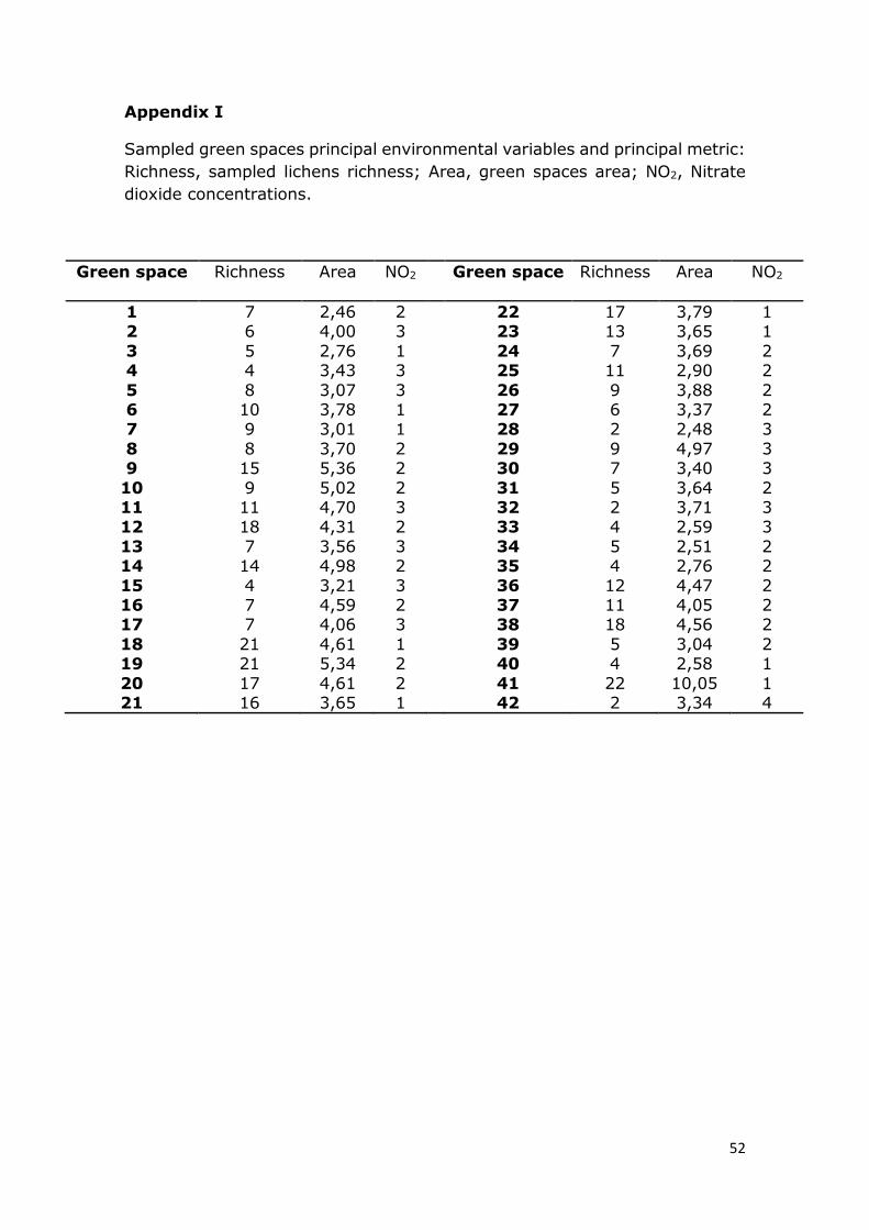
52

Appendix I

Sampled green spaces principal environmental variables and principal metric:

Richness, sampled lichens richness; Area, green spaces area; NO2, Nitrate

dioxide concentrations.

Green space Richness Area NO2 Green space Richness Area NO2

1 7 2,46 2 22 17 3,79 1 2 6 4,00 3 23 13 3,65 1

3 5 2,76 1 24 7 3,69 2 4 4 3,43 3 25 11 2,90 2

5 8 3,07 3 26 9 3,88 2 6 10 3,78 1 27 6 3,37 2 7 9 3,01 1 28 2 2,48 3

8 8 3,70 2 29 9 4,97 3 9 15 5,36 2 30 7 3,40 3

10 9 5,02 2 31 5 3,64 2 11 11 4,70 3 32 2 3,71 3 12 18 4,31 2 33 4 2,59 3

13 7 3,56 3 34 5 2,51 2 14 14 4,98 2 35 4 2,76 2

15 4 3,21 3 36 12 4,47 2 16 7 4,59 2 37 11 4,05 2 17 7 4,06 3 38 18 4,56 2

18 21 4,61 1 39 5 3,04 2 19 21 5,34 2 40 4 2,58 1

20 17 4,61 2 41 22 10,05 1 21 16 3,65 1 42 2 3,34 4

53

Appendix II

List of species found in the total green spaces. Nomenclature follows Nimis

& Martellos (2008).

Candelaria concolor

Candelariella xanthostigma

Caloplaca citrina

Chrysotrix candelaris

Diploicia canescens

Evernia prunastri

Enterographa crassa

Flavoparmelia caperata

Hyperphyscia adglutinata

Lecania cyrtella

Lecania cuprea

Lecania naegelli

Lecanographa amylacea

Lecanora chlarotera

Lecanora expallens

Lecanora horiza

Lecanora pulicaris

Lecidella elaechroma

Lepraria sp.

Parmotrema hypoleucinum

Parmotrema perlatum

Parmotrema reticulatum

Pertusaria amara

Pertusaria pertusa

Phaeophyscia endophoenicea

Phaeophyscia hirsuta

Phaeophyscia orbicularis

Physcia adscendens

Physcia clementei

Physcia dubia

Physcia leptalea

Pyscia tenella

Physcia tribacioides

Physconia grisea

Punctelia borreri

Ramalina lacera

Ramalina farinacea

Ramalina fastigiata

Rinodina capensis

Schismatomma decolorans

Xanthoria parietina

Waynea stoechadiana

54

Appendix III

Air quality model residuals – Normal probability plot of residuals (a) and

histogram of raw residuals (b).

55

Appendix IV

Variables with lower correlations with the considered metrics. HBD,

Diameter Breast hight (used as a surrogate of tree age); U100, Urban

density within a 100m buffer; U200, Urban density within a 200m buffer;

NVeg, ; NDVIc, NDVI measured at the green space center; PSR, Potential

solar radiation ; Slop, slope ; Alt, . The symbol * represents significance at

p<0,05; ** represents significance at p<0,01; *** represents significance

at p<0, 001.

DBH U100 U200 NVeg NDVIc PSR Slop Dist

Richness -0,070 -0,265 -0,324 -0,154 0,347 *

-0,245 0,237 0,237

FR -0,060 -0,320 -0,370 -0,202 0,334

*

-0,240 0,235 0,235

LDVt

-0,436

**

-0,516

***

-0,521

***

-0,429

**

0,304 -0,082 0,135 0,135

LDVnit -0,272 -0,337 -0,397 -0,328

*

-0,142 0,065 0,119 0,119

LDVmes -0,277 -0,477 **

-0,459 **

-0,287 0,422 *

-0,087 0,084 0,084

LDVolig -0,220 -0,348 -0,379 -0,298 0,335 *

0,033 0,186 0,186

LDVHygr -0,173 -0,310 -0,327 -0,013 0,349* -0,175 0,202 0,202

LDVmesh 0,007 -0,170 -0,127 -0,034 0,365

*

-0,114 0,082 0,082

LDVxer -0,400 **

-0,380 -0,432 **

-0,393 **

0,056 0,078 0,076 0,076

LDVcrust -0,371 ***

-0,518 ***

-0,517 ***

-0,413 **

0,084 -0,148 0,092 0,092

LDVfoln -0,263 -0,370 -0,382 -0,250 0,007 0,048 0,026 0,026

LDVfolbr -0,276 -0,217 -0,212 -0,019 0,434

*

-0,218 0,238 0,238

LDVfrut -0,314 ***

-0,049 -0,105 -0,070 0,223 -0,046 0,386 0,385

LDVsq 0,058 -0,085 -0,059 -0,066 0,140 -0,079 0,119 0,119

LDVlepr -0,315 ***

-0,186 -0,139 -0,091 0,316 *

-0,099 0,138 0,138

56

Appendix V

Plot of green spaces area (Area) and the percentage of lichen species

richness increase (Richness).