1

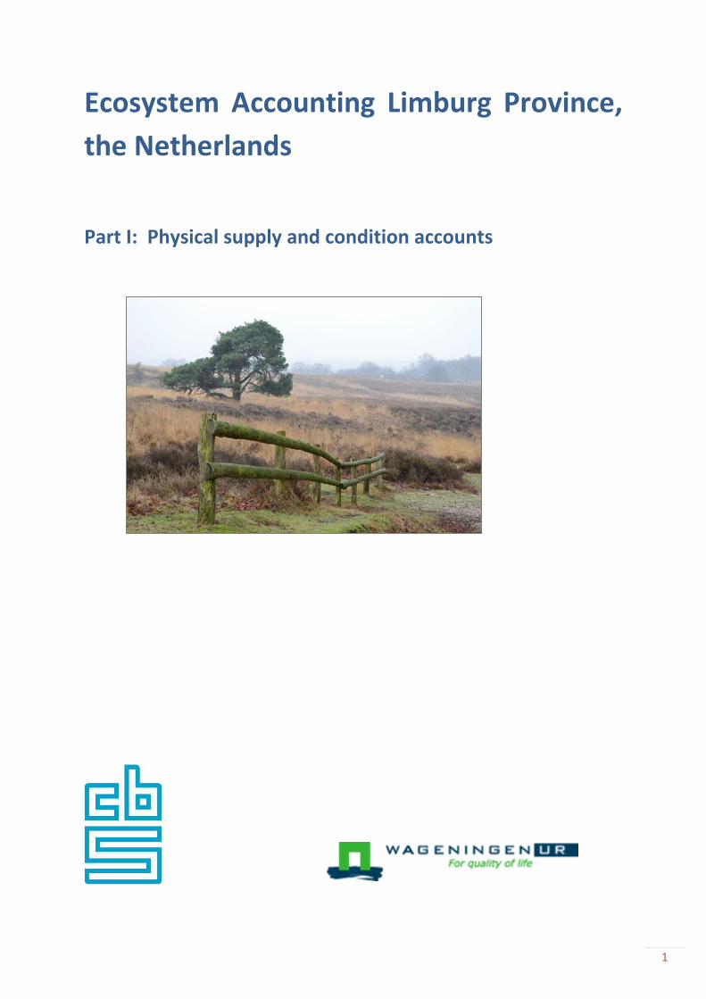
Ecosystem Accounting Limburg Province,

the Netherlands

Part I: Physical supply and condition accounts

2

3

This report presents the results of a pilot project which was carried out by Statistics Netherlands

and Wageningen University. Funding was provided by the Ministries of Economic Affairs and of

Infrastructure and the Environment.

Authors

Part I: Rixt de Jong, Bram Edens, Niek van Leeuwen and Sjoerd Schenau, Statistics Netherlands (CBS)

Roy Remme and Lars Hein, Wageningen University

Part II: Roy Remme and Lars Hein, Wageningen University

Front page image: Matthias Schröter

4

Abstract

Worldwide, ecosystems and their biodiversity are under severe environmental pressure.

Consequently, the supply of valuable services provided by these ecosystems, such as the

provisioning of timber, water regulation, air filtration or recreation, is being reduced or lost.

Ecosystem accounting aims to quantify and monitor the interdependence between ecosystems

(and their services) and economic activities, in an internationally consistent manner. The

accounting system is based on tracking changes in the supply and economic use of ecosystem

services. It also aims to monitor the extent and condition of ecosystems, which is needed to

identify the causes for changes in ecosystem services supply. The methodology was developed by

an international group of experts under auspices of the UN Committee of Experts on

Environmental-Economic Accounting (UNCEEA Statistical Committee) UN et al. (2014). Following

endorsement by the UN Statistical Committee, ecosystem accounting is now part of the

international framework of the UN the System of Environmental Economic Accounts. In two

reports we describe the results of a pilot study on ecosystem accounting in Limburg Province, the

Netherlands. The current report focusses on the physical supply of ecosystem services and on

ecosystem condition indicators. The second report describes the monetary valuation approach and

monetary supply and use tables for the same ecosystem services. The two reports are thus

complimentary.

1. Introduction

Ecosystems provide services, known as ecosystem services, that contribute to national economies

and human welfare. For example, soils and vegetation form sinks for carbon dioxide, the air is filtered

by vegetation and dunes protect against coastal floods and provide space for recreation and

education. The supply and sustainability of such services depend on ecosystem condition and extent.

Ecosystem accounting was developed in recognition of the vital importance of these ecosystem

services and provides a tool for consistent monitoring and quantifying the supply and use of

ecosystem services. This is highly relevant because ecosystems and their biodiversity are subject to

increasing environmental pressures worldwide, a trend that was already signalled and described in

the Brundtland Report in 1987 (WCED, 1987). These environmental pressures are in part related to

expanding human populations and increased economic activities. The increased demand for food and

materials, fuel and living space lead to pollution, severe land degradation, the transition of natural

areas to cultivated land and to the loss of biodiversity (e.g. Butchart et al., 2010). In addition, climate

change may severely impact ecosystems (IPCC, 2014). In time, these pressures may lead to a

reduction of the supply of ecosystem services, which could have major consequences for human

welfare and the economy.

Many nations now recognise the vulnerability and value of their ecosystems and have applied

conservation and protection measures (e.g. TEEB, 2010). Currently, however, neither the ecosystem

contributions to economies, nor the losses or increases of services are accounted for in national and

international statistics. To fill this gap, the United Nations Statistics Department (UNSD) launched the

System of Environmental Economic Accounts – Experimental Ecosystem Accounting in 2014 (SEEA-

5

EEA, UN et al., 2014). This publication provides provisional guidelines and encourages nations to

experiment with Ecosystem Accounting using methods that are consistent with the System of

National Accounts (SNA). It is a novel approach to measure the contribution of ecosystem services to

national economies. The SEEA-EEA were developed with the purpose to ‘better inform individual and

social decisions concerning the use of the environment by developing information in a structured and

internationally consistent manner, based on recognition of the relationship between ecosystems and

economies and other human activity’ (UN et al., 2014). The ecosystem accounting system is further

explained in section 2.

This report first provides an overview of the most important concepts of the SEEA-EEA guidelines and

the project aims. Next, we present the methods and results for the developed maps, the physical

supply of ecosystem services and for the conceptual condition account. Finally we discuss the

implications of the findings and provide recommendations for future work. All information on the

monetary valuation of ecosystem services (methods, results, discussion and conclusions) are

included in Part II of the current report.

2. Theoretical background and project aims

2.1 The theoretical framework of Ecosystem Accounting: the SEEA EEA approach

The ‘System of Environmental Economic Accounts – Experimental Ecosystem Accounting (SEEA-EEA)’

was developed and published under the auspices of the-United Nations Committee of Experts on

Environmental-Economic Accounting (UNCEEA), as mandated by the UN Statistics Committee at its

38th session in 2007. The UNCEEA is a governing body comprising senior representatives from

national statistical offices and international organizations. It is chaired by a representative of one of

the country members of the Committee. The United Nations Statistics Division serves as Secretariat

for UNCEEA (UN et al., 2014). SEEA EEA was based on the inputs of professionals from multiple

disciplines such as economists, biologists, modellers and statisticians. International organisations

such as the UNSD, World Bank, UNEP (United Nations Environmental programme), Eurostat, EEA

(European Environmental Agency) and NGO’s were also involved. Ecosystem accounting aims to

identify changes in the condition and extent of ecosystem units and the resulting changes in the

quantity and - where possible - monetary value of the supplied ecosystem services. This provides

insight in the full economic use of and dependencies on natural capital, and how these may change

through time. Consequently, Ecosystem Accounting provides a powerful tool for monitoring the

economic impacts of pressures as well as protection measures on ecosystems and the subsequent

changes in ecosystem services.

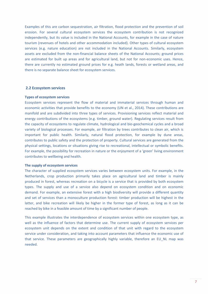
The SEEA EEA ecosystem accounting model is shown in figure 2.1.1) (source: UN et al, 2014). Starting

at the bottom of the figure the model is based around accounting for an ecosystem asset that is a

defined spatial area. Each ecosystem asset has a range of relevant ecosystem characteristics and

processes that together describe the functioning of the ecosystem. The accounting model proposes

that the stock and changes in stock of ecosystem assets is measured by considering the ecosystem

6

asset’s extent and condition which can be done using indicators of the relevant ecosystem’s area,

characteristics and processes. Each ecosystem asset generates a set of ecosystem services which, in

turn, contribute the production of benefits. Benefits may be goods or services currently included in

the economic production boundary of the SNA, SNA benefits, or they may be benefits received by

individuals that are not produced by economic units (e.g. clean air). These are non-SNA benefits.

Benefits, both SNA and non-SNA, contribute to individual and societal well-being or welfare.

2.1.1 Ecosystem accounting model (UN et al., 2014 Figure 2.2)

The SEEA –EEA is thus based on the dual concepts of ecosystem assets and ecosystem services. The

accounting logic for SEEA EEA is as follows: ecosystem extent and condition determine the possible

supply of ecosystem services to the economy (capacity), whereas the actual supply also depends on

the demand for services (ES use). Next, following the SNA methodology and definitions, supply

equals use. Accounting tables are then developed for ecosystem condition (including extent), and for

the supply and use of ecosystem services (e.g. kg · yr -1), in physical terms. In addition, the monetary

supply of ecosystem services (€ · yr -1) can be analysed (ES supply and ES Use). In the current study,

the physical supply and use tables and the condition table were developed and populated where

possible. In addition, monetary supply and use tables were developed by Wageningen University (see

Report II).

The SEEA EEA also provides information on the concepts of monetary asset and capacity accounts.

These potentially provide insight into the balance of ecosystem services and in the sustainability of

their use. In addition, a set of supporting accounts (biodiversity, carbon, land, water) was envisaged

in the guidelines. For example, biodiversity has been recognised as a key ecosystem property and

therefore a separate account for biodiversity was proposed to enable the monitoring of biodiversity

over time in a consistent manner. Key indicators from this account form input for the condition

account (UNEP-WCMC, 2015). However, these accounts were outside the scope of the current pilot

project.

The relation of the ecosystem accounts to the National Accounts is complex. SEEA EEA was

developed to specifically address ecosystem contributions to national economies, and to thereby

show the dependence of economic activities on ecosystems. A number of ecosystem services are

currently already included in the National Accounts, without being recognized separately as

contributions from ecosystems. Examples of such services are the contributions of ecosystems to e.g.

crop, fodder and timber production. Regulating services are not included in the National Accounts.

7

Examples of this are carbon sequestration, air filtration, flood protection and the prevention of soil

erosion. For several cultural ecosystem services the ecosystem contribution is not recognized

independently, but its value is included in the National Accounts, for example in the case of nature

tourism (revenues of hotels and other accommodation included). Other types of cultural ecosystem

services (e.g. nature education) are not included in the National Accounts. Similarly, ecosystem

assets are excluded from the non-financial balance sheets of the National Accounts; ground prices

are estimated for built up areas and for agricultural land, but not for non-economic uses. Hence,

there are currently no estimated ground prices for e.g. heath lands, forests or wetland areas, and

there is no separate balance sheet for ecosystem services.

2.2 Ecosystem services

Types of ecosystem services

Ecosystem services represent the flow of material and immaterial services through human and

economic activities that provide benefits to the economy (UN et al., 2014). These contributions are

manifold and are subdivided into three types of services. Provisioning services reflect material and

energy contributions of the ecosystems (e.g. timber, ground water). Regulating services result from

the capacity of ecosystems to regulate climate, hydrological and bio-geochemical cycles and a broad

variety of biological processes. For example, air filtration by trees contributes to clean air, which is

important for public health. Similarly, natural flood protection, for example by dune areas,

contributes to public safety and the protection of property. Cultural services are generated from the

physical settings, locations or situations giving rise to recreational, intellectual or symbolic benefits.

For example, the possibility for recreation in nature or the enjoyment of a ‘green’ living environment

contributes to wellbeing and health.

The supply of ecosystem services

The character of supplied ecosystem services varies between ecosystem units. For example, in the

Netherlands, crop production primarily takes place on agricultural land and timber is mainly

produced in forest, whereas recreation on a bicycle is a service that is provided by both ecosystem

types. The supply and use of a service also depend on ecosystem condition and on economic

demand. For example, an extensive forest with a high biodiversity will provide a different quantity

and set of services than a monoculture production forest: timber production will be highest in the

latter, and bike recreation will likely be higher in the former type of forest, as long as it can be

reached by bike in a feasible amount of time by a significant number of people.

This example illustrates the interdependence of ecosystem services within one ecosystem type, as

well as the influence of factors that determine use. The current supply of ecosystem services per

ecosystem unit depends on the extent and condition of that unit with regard to the ecosystem

service under consideration, and taking into account parameters that influence the economic use of

that service. These parameters are geographically highly variable, therefore an EU_NL map was

needed.

8

2.3 Project objectives

The objectives of the project are listed below, followed by a short description.

1) Develop and compile land accounts (use and activity) for the Netherlands: The spatial

delineation of ecosystem types lies at the basis of all subsequent ecosystem accounts. In a national

accounting sense, ecosystem units are the equivalent of economic sectors. Each sector (ecosystem

unit) produces a certain set of (ecosystem) services and products, the quantity of which depends on

the size (extent) of the unit and its condition. Therefore, a highly detailed map showing ecosystem

units in the Netherlands was essential to carry the project forward (the Ecosystem Units or ‘EU_NL’

map). In addition, an economic users (ISIC) map was developed to identify the economic users of

location-specific services.

2) Carry out an inventory of available data for the Netherlands, on ecosystem services, asset

and condition: For the Netherlands, a large amount of data and maps containing information on

ecosystem services, condition and assets are already available. An inventory was needed to find all

suitable data (e.g. of sufficient quality and resolution, no double counting, transparency on modelling

assumptions, etc.) and to establish the possibility of developing a comparison over time on

ecosystem extent and services supply.

3) Develop and conceptually design Natural Capital Accounting Tables: In the current SEEA

EEA guidelines, the design and development of accounting tables is not made explicit for all accounts.

In addition, the potential content of the tables depends on data availability and quality, which is

country specific.

4) Populate the proposed tables for a chosen area, for a selected number of services and

ecosystem types, in physical and where possible monetary data: Populating the accounts with

all possible data was the main objective of this pilot project. Accounts for Limburg were populated

for a selection of 8 (physical supply table) or 7 (monetary supply table, monetary use table)

ecosystem services, for 31 ecosystem units. In addition, a test-case was developed for hedonic

pricing of the amenity service (green living environment).

All objectives were achieved within this project.

2.4 Relation to other projects on Natural Capital Accounting

The ecosystem accounting project for Limburg is complementary to other initiatives carried out in

the field of Natural Capital Accounting. The project builds upon the Ecospace project of Wageningen

University. Ecospace is a European Research Council funded project aimed at developing and testing

methods for ecosystem accounting. The project started in 2010 and was finalized in November 2015.

In this project physical and monetary ecosystem accounts, covering both capacity and services, were

developed for three test sites: Limburg province, Telemark province, Norway and Central Kalimantan

province, Indonesia. In each area, around 8 ecosystem services were mapped, analysed and, in the

case of Limburg and Central Kalimantan, valued in monetary terms. Outcomes of the project have

been presented in the form of scientific papers (10 papers published to date) and in terms of

contributions to discussions on SEEA and ecosystem accounting with the World Bank, UNSD, EEA and

9

Eurostat. The Atlas Natural Capital (RIVM, funded by Min. Infrastructure and the Environment)

provides essential information on the geographical extent and characteristics of a number of

ecosystem services and ecosystem condition. There is a strong collaboration between the project

partners and RIVM and other contributors to the Atlas to ensure that presently available information

in the Atlas is incorporated in the ecosystem accounts, and that future developments of the Atlas

are, where possible, mutually beneficial. The ESD report by Alterra (Wageningen) provides semi-

quantitative information (e.g. percentage of demand fulfilled by natural supply) on a large number of

ecosystem services in the Netherlands. The Material Monitor+ by Statistics Netherlands (initiative by

Min. EZ) project describes a wide range of policy questions related to the extraction, use and scarcity

of natural resources as well as a range of related topics, such as the circular economy and ecosystem

services. The Monitor focusses exclusively on flows that can be expressed in tonnes or kg’s of

material. The MAES project (by BISE, a partnership between the European Commission and the

European Environment Agency) aims to support the knowledge base for the implementation of the

EU 2020 Biodiversity Strategy. The database contains maps of ecosystem services on a regional,

national, European and global scale, presented for a range of ecosystem types.

3. Methods

3.1 Ecosystem Unit (EU_NL) Map

Ecosystem accounting was designed to be spatially explicit: ecosystem services and conditions are

spatially modelled or mapped, or otherwise attributed to spatial units. This implies that both the

physical and monetary supply tables are based on mapped ecosystem services as much as possible.

Within our current project an Ecosystem Unit (EU_NL) map was developed for the Netherlands. This

map is essential to model and quantify ecosystem services and to assign supplied services spatially to

a set of ecosystem units. Therefore, the EU_NL map reflects a division into ecosystem units that was,

as far as possible, consistent with other mapping efforts (MAES, SEEA EEA Ecosystem Unit types, see

section 3.2), as well as practical for the purpose of modelling ecosystem services. The map needs to

provide full spatial coverage, implying that all built up terrain is also assigned to a set of ecosystem

units. The aim was to provide a detailed map that reflects land use and vegetation properties at a

high level of detail. On top of that, essential location features were mapped for two natural assets:

coastal dune areas and river floodplains. For the Netherlands, both assets are of critical importance

in the protection against coastal and river floods, on local, regional and national scales. Information

on all ecosystem units within these regional scale features is also available at a lower legend level.

The EU_NL map was based on a strategic combination of a number of maps and datasets covering

the Netherlands: the cadastral map, agricultural crops grown, address based business register,

addresses of buildings, the basic topographical registry and land use statistics for the Netherlands.

Maps were combined following a strict hierarchical approach. Once a unit is assigned, it can no

longer be changed. For built up areas, the cadastral unit was taken as the base unit. However, where

cadastral parcels were dissected by roads, water or railways, the smaller parcels were taken as the

initial unit.

First all water was assigned. In a series of following steps, the different units for built up areas

(residential areas, business areas etc.) were assigned, followed by roads and other paved surfaces.

10

For non-residential built-up areas economic use was decisive, so that the map provides information

on whether built up terrain is used by main ISIC sections such as government, the services sector,

manufacturing etc. Next, for all agricultural land, the agricultural crops grown in 2013 were used to

divide parcels into perennial and non-perennial crops. Meadows for grazing were defined based on

the same registry. Natural grasslands were defined based on the position of meadows; grazing

meadows within the EHS (National Ecological Network) were considered to represent this category.

Finally, all unpaved surfaces without agricultural activities remained. These were assigned using the

basic topographical registry for remaining types of land cover and the land use map for functional

areas such as unpaved agricultural and nature roads. A number of other delineations of policy-based

locations (Natura 2000, delineation of river floodplains) are superimposed on the EU_NL map. Thus,

the map is multi-layered: details on land use within e.g. river floodplains are still available, so that

e.g. agricultural production within this legend unit can be calculated from this map. The resulting

map is a highly detailed polygon map that also contains fine line elements (e.g. gravel paths and

hedgerows wider than 6m). It contains all available information on agricultural land use and detailed

information on natural and semi-natural areas.

3.2 Relation to other international mapping efforts

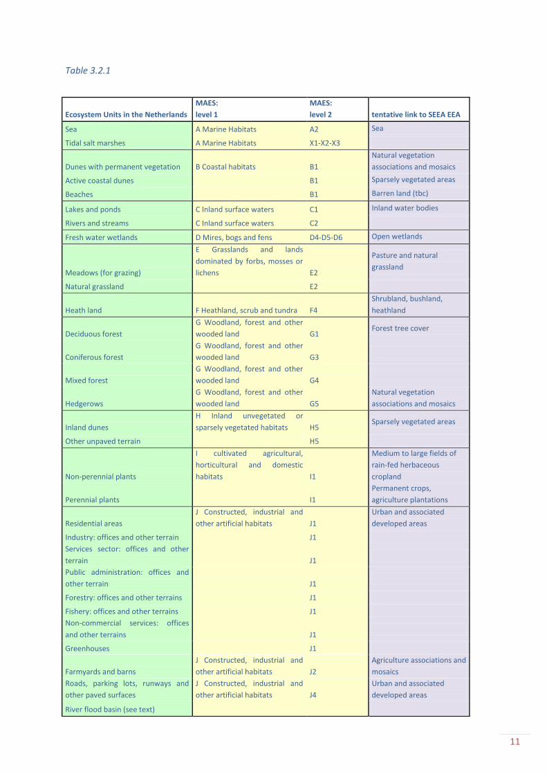
The current classification can be translated into the MAES classification level 2 without any major

obstacles, as shown in Table 3.2.1. The classification developed for the EU map is, however, a bit

more detailed (see MAES levels B, E, H, I and J) and places specific focus on the river floodplains and

dunes. Because the map is multi-layered, it is easy to convert the river floodplain areas into MAES

units, if so desired.

The ecosystem types suggested in the SEEA EEA (Table 3.2.1) are somewhat similar to those in MAES,

however, the linkages are not always clear and the classifications in the SEEA EEA appear to be

overlapping. For example, SEEA EEA recognizes ‘open wetlands’ separately, whereas a large number

of wetland types (e.g. bogs and mires) may be covered with (sparse to dense) trees and shrubs. In

addition, SEEA EEA distinguishes between rain fed versus irrigated cropland. It is not clear what to do

with temporarily irrigated lands, where the occurrence of irrigation depends on the rainfall in a

particular season or year. In general, the SEEA EEA classification does not generally provide suitable

classes for the Netherlands, and in its current form it does not contain enough detail for the analyses

that were required in this study. However, at a high aggregation level the classifications can be linked

so that reporting at the international level would be possible with the classes used in the pilot study,

as shown in the Table above.

11

Table 3.2.1

Ecosystem Units in the Netherlands

MAES:

level 1

MAES:

level 2 tentative link to SEEA EEA

Sea A Marine Habitats A2 Sea

Tidal salt marshes A Marine Habitats X1-X2-X3

Dunes with permanent vegetation B Coastal habitats B1

Natural vegetation

associations and mosaics

Active coastal dunes B1 Sparsely vegetated areas

Beaches B1 Barren land (tbc)

Lakes and ponds C Inland surface waters C1 Inland water bodies

Rivers and streams C Inland surface waters C2

Fresh water wetlands D Mires, bogs and fens D4-D5-D6 Open wetlands

Meadows (for grazing)

E Grasslands and lands

dominated by forbs, mosses or

lichens E2

Pasture and natural

grassland

Natural grassland E2

Heath land F Heathland, scrub and tundra F4

Shrubland, bushland,

heathland

Deciduous forest

G Woodland, forest and other

wooded land G1 Forest tree cover

Coniferous forest

G Woodland, forest and other

wooded land G3

Mixed forest

G Woodland, forest and other

wooded land G4

Hedgerows

G Woodland, forest and other

wooded land G5

Natural vegetation

associations and mosaics

Inland dunes

H Inland unvegetated or

sparsely vegetated habitats H5 Sparsely vegetated areas

Other unpaved terrain H5

Non-perennial plants

I cultivated agricultural,

horticultural and domestic

habitats I1

Medium to large fields of

rain-fed herbaceous

cropland

Perennial plants I1

Permanent crops,

agriculture plantations

Residential areas

J Constructed, industrial and

other artificial habitats J1

Urban and associated

developed areas

Industry: offices and other terrain J1

Services sector: offices and other

terrain J1

Public administration: offices and

other terrain J1

Forestry: offices and other terrains J1

Fishery: offices and other terrains J1

Non-commercial services: offices

and other terrains J1

Greenhouses J1

Farmyards and barns

J Constructed, industrial and

other artificial habitats J2

Agriculture associations and

mosaics

Roads, parking lots, runways and

other paved surfaces

J Constructed, industrial and

other artificial habitats J4

Urban and associated

developed areas

River flood basin (see text)

12

3.3 Economic Users map

To identify the users of ecosystem services, two approaches were applied: 1) conceptual selection of

users, and 2) geographical allocation of users, with the help of an Economic Users map. The

Economic Users map was based on the same data and delineations as the EU_NL map (see Fig. 4.2.1).

The classification for the economic users map was based on the ISIC classification for businesses (NL:

SBI with 21 sections (A-U). In addition to these ISIC units, four non-economic land use types were

distinguished to ensure full map coverage: roads, households , water and (semi) natural areas. Using

this map, it is possible to identify the users of ecosystem services that are spatially explicit, such as

the users (beneficiaries) of flood protection or noise reduction.

3.4 Physical supply of ecosystem services

Remme et al. (2014) provide a detailed description of the modelling approaches used to estimate the

physical supply of the selected ecosystem services. For the current study, the approach was updated

by using the newly developed EU_NL map as a basis and new data where relevant. In summary (all

based on Remme et al., 2014), the provisioning of crops was modelled for the most common crop

types in the base registry for crops grown (> 10 crop types for human consumption). Fodder was

modelled using data on yields of two main sources of fodder: maize and pasture. Groundwater

provisioning was modelled for eleven (shallow) groundwater extraction wells and surrounding

protected areas, where groundwater is extracted to supply drinking water. Meat obtained by hunting

was modelled for 43 hunting districts in Limburg for wild boar (Sus scrofa) and European roe deer

(Capreolus capreolus).The regulating service capture of PM10 reflects the filtering of particulate

matter from the air. It was modelled using published values for PM10 capture by different types of

land cover, combined with ambient PM10 concentration maps. Terrestrial carbon sequestration is the

storage of carbon in vegetation and soils. It was mapped using published data on carbon storage in

different land cover types. The cultural service recreation by bike was modelled using the national

cycle path network, a map of attractiveness of the landscape and population density. The total

number of recreational biking trips (excluding race biking and mountain biking) was known from

previous publications. Nature tourism was modelled using data on accommodation capacity and

visiting statistics for three regions in Limburg. For more details see Remme et al., 2014.

3.5 The extent account and the physical Supply and Use tables

All tables were designed according to SEEA-EEA guidelines. The ecosystem extent account for

Limburg Province was compiled based on the EU_NL map. This presents a major refinement

compared to the previous study carried out for Limburg, because ecosystem services can be linked to

a more detailed and more accurate map. Ecosystem supply was analysed for each ecosystem unit

(columns) and for all ecosystem services (rows) that were included in this study. The physical

quantities of the services supply were based directly on the modelled ecosystem services maps. So,

to determine the physical supply of ecosystem services per ecosystem unit, for example the physical

supply of the service fodder production, the physical supply of fodder was modelled based on the

information available in the EU_NL map.

13

The Use tables were constructed differently. Although a detailed economic users map (based on the

ISIC registry) was developed within this project, none of the ecosystem services that were included in

this study had spatially explicit economic users, as would have been the case for e.g. flood protection

and noise reduction. Therefore, users were defined depending on the physical and monetary model

characteristics, following the ISIC classification as much as possible. Because the physical use table

was based directly on the monetary use table (shown in report II), it is not shown here.

3.6 Conceptual Condition Account

The ecosystem condition account records information on the various characteristics that reflect

the condition or quality of an ecosystem. (SEEA EEA; UN et al, 2014).The purposes of a condition

account can be manifold: it summarizes which condition indicators are relevant for the functioning of

a given ecosystem, it can include condition indicators that control the supply of ecosystem services,

or it can contain condition indicators that are more explicitly politically relevant. At the very least, it

should include those indicators that, if they change over time, lead to a change in the supply of

ecosystem services (UN et al., 2014). This latter group includes all parameters that were used in the

development of the biophysical ecosystem service supply model. For example, for the modelling of

bicycle tourism, input parameters into the model included population density, attractiveness of the

landscape and the location of the Dutch national biking network. Out of these, only the

attractiveness of the landscape may be interesting for policy reasons, whereas none of these are vital

indicators for the functioning of the ecosystems themselves. In short, we propose that three sets of

condition indicators should be considered, which is also aligned with the forthcoming Technical

Recommendations for SEEA EEA (to be published by UNSD early 2016). Note that the description of

the indicators is based upon the upcoming Technical Recommendations as well as our experiences in

the pilot project:

a. Physical state indicators: These indicators concern the recording of relatively fixed characteristics

of ecosystem assets such as measures of soil type, slope, altitude, climate and rainfall. These are

important inputs in the modelling of ecosystem services, but by themselves not necessarily policy-

relevant. They may be included in an Annex of the accounts.

b. Environmental state indicators: The second group reflects measures of impacts or pressures on

the environmental state, for example, measures of pollution, emissions or waste. Accounting for

these flows is described in the SEEA Central Framework although more spatial detail is required

for ecosystem accounting purposes. While primarily needed for measuring regulating services,

they will also be relevant in the assessment of ecosystem condition. This group of indicators may

also be of interest from a policy monitoring perspective.

c. Ecosystem state indicators: These measures reflect for example, the degree of fragmentation,

leaf area index, nutrient status of the ecosystem, biodiversity, the attractiveness of the landscape

or the degree of ‘naturalness’ of vegetation. These indicators are of vital importance to

understand how the ecosystem is currently functioning and how the ecosystem can supply

ecosystem services. This information is also relevant for specifying biodiversity conservation

priorities, however not all indicators (such as leaf area index) are policy relevant.

The condition account should, like all accounts in this report, be based on geographically explicit

information that can be updated at a regular basis.

14

4. Results and interpretation

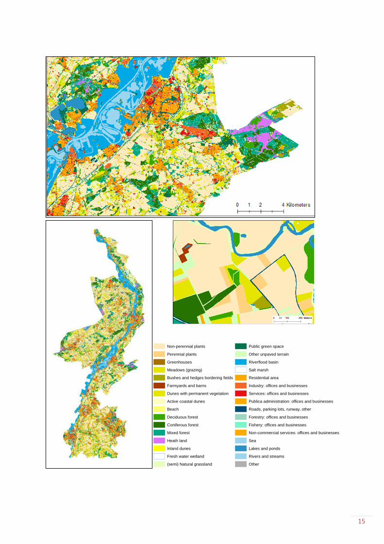
4.1 EU_NL map

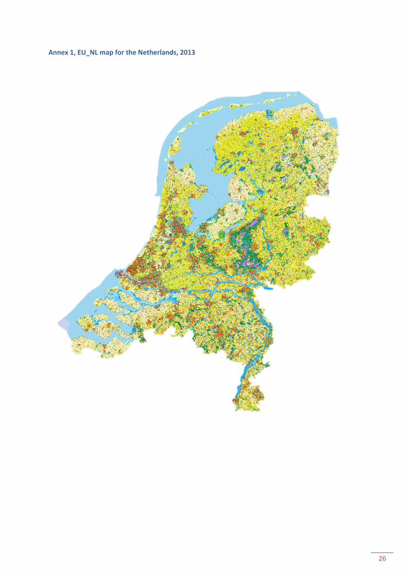
The EU_NL map was constructed for the Netherlands (see Annex). The map has already been made

available to the Atlas Natural Capital (RIVM) to be used as the basis for further ecosystem service

modelling, and will be made publicly available in 2016. Figure 4.1.1 provides examples of the many

different units that are discerned and the high level of detail. The province of Limburg is shown in

Figure 4.1.1b. Figure 4.1.1a shows a part of the map for the municipality of Roerdalen in the central

part of Limburg. National Park ‘de Meinweg’ is located at the border with Germany and is

characterized by deciduous, mixed and coniferous forest types and heathland. The city of Roermond

(to the West) shows up as a mixture of all built up ecosystem unit types. It lies directly along the river

Maas. The streambed of the river Maas and adjacent artificial lakes (from gravel extractions, all in

light blue) and the entire floodplain (the area where flooding may occur during runoff peaks, shown

in dark blue) are shown in detail. In Limburg a number of villages were built within the floodplain of

the river as can also be seen in this figure. Parts of these villages are situated on naturally higher

ground, whereas other parts and villages in Limburg are situated at lower elevations and were

flooded in 1993 and 1995. Figure 4.1.1c provides an example of the high level of detail by showing a

part of the small river Roer. The Roer has several meander cut-offs (oxbow lakes) that are overgrown

with deciduous trees, and small sandy islands within the streambed. Gravel roads in this rural area

also show up clearly (light green lines).

Next page: Figure 4.1.1, showing the EU_NL map for: a) the municipalities of Roermond (centre) and

Roerdalen (east), b) Limburg province, and c) a detail of the stream the Roer.

15

Non-perennial plants

Perennial plants

Greenhouses

Meadows (grazing)

Bushes and hedges bordering fields

Farmyards and barns

Dunes with permanent vegetation

Active coastal dunes

Beach

Deciduous forest

Coniferous forest

Mixed forest

Heath land

Inland dunes

Fresh water wetland

(semi) Natural grassland

Public green space

Other unpaved terrain

Riverflood basin

Salt marsh

Residential area

Industry: offices and businesses

Services: offices and businesses

Publica administration: offices and businesses

Roads, parking lots, runway, other

Forestry: offices and businesses

Fishery: offices and businesses

Non-commercial services: offices and businesses

Sea

Lakes and ponds

Rivers and streams

Other

16

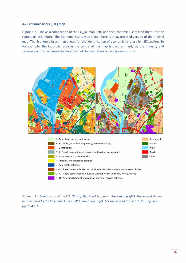
4.2 Economic Users (ISIC) map

Figure 4.2.1 shows a comparison of the EU_NL map (left) and the Economic Users map (right) for the

same part of Limburg. The Economic Users map shown here is an aggregated version of the original

map. The Economic Users map allows for the identification of economic land use by ISIC section. So

for example, the industrial area in the centre of the map is used primarily by the industry and

services sections, whereas the floodplain of the river Maas is used for agriculture.

Figure 4.2.1 Comparison of the EU_NL map (left) and Economic Users map (right). The legend shown

here belongs to the Economic Users (ISIC) map to the right. For the legend to the EU_NL map, see

figure 4.1.1.

A Agriculture, forestry and fishing

B - E Mining, manufacturing, energy and water supply

F Construction

G - I Retail, transport, accomodation and food service activities

J Information and communication

K Financial and insurance activities

L Real estate activities

M - N Professional, scientific, technical, administrative and support service activities

O - Q Public administration, education, human health and social work activities

R - U Arts, entertainment, recreational and other service activities

Residential

Nature

Water

Roads

Other

17

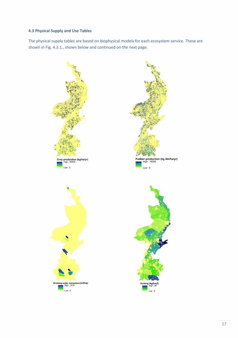
4.3 Physical Supply and Use Tables

The physical supply tables are based on biophysical models for each ecosystem service. These are

shown in Fig. 4.3.1., shown below and continued on the next page.

18

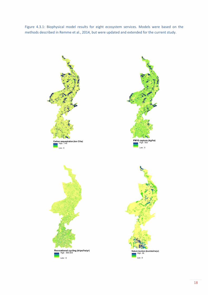
Figure 4.3.1: Biophysical model results for eight ecosystem services. Models were based on the

methods described in Remme et al., 2014, but were updated and extended for the current study.

19

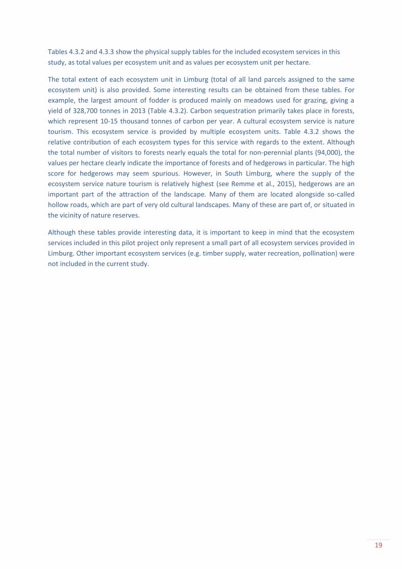
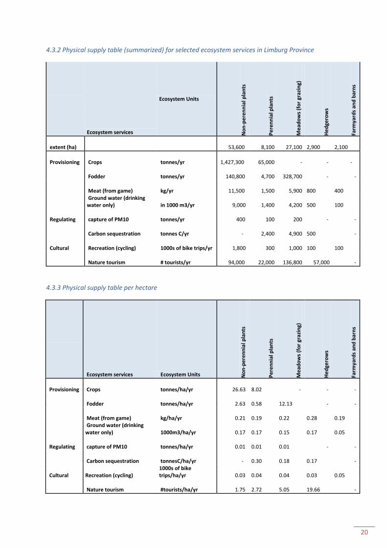
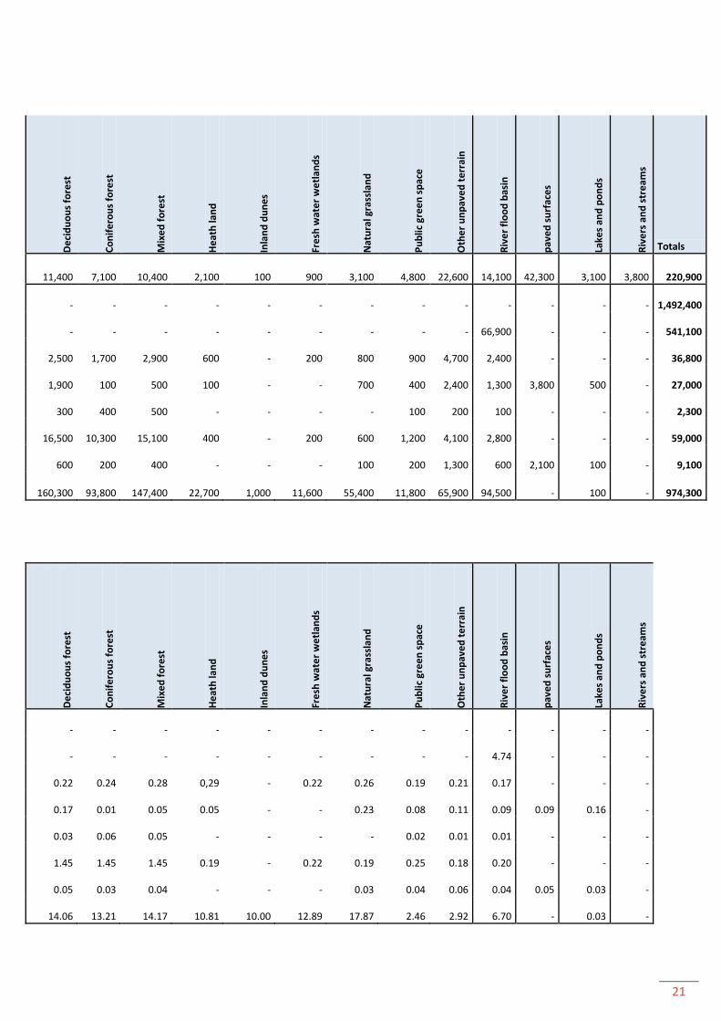
Tables 4.3.2 and 4.3.3 show the physical supply tables for the included ecosystem services in this

study, as total values per ecosystem unit and as values per ecosystem unit per hectare.

The total extent of each ecosystem unit in Limburg (total of all land parcels assigned to the same

ecosystem unit) is also provided. Some interesting results can be obtained from these tables. For

example, the largest amount of fodder is produced mainly on meadows used for grazing, giving a

yield of 328,700 tonnes in 2013 (Table 4.3.2). Carbon sequestration primarily takes place in forests,

which represent 10-15 thousand tonnes of carbon per year. A cultural ecosystem service is nature

tourism. This ecosystem service is provided by multiple ecosystem units. Table 4.3.2 shows the

relative contribution of each ecosystem types for this service with regards to the extent. Although

the total number of visitors to forests nearly equals the total for non-perennial plants (94,000), the

values per hectare clearly indicate the importance of forests and of hedgerows in particular. The high

score for hedgerows may seem spurious. However, in South Limburg, where the supply of the

ecosystem service nature tourism is relatively highest (see Remme et al., 2015), hedgerows are an

important part of the attraction of the landscape. Many of them are located alongside so-called

hollow roads, which are part of very old cultural landscapes. Many of these are part of, or situated in

the vicinity of nature reserves.

Although these tables provide interesting data, it is important to keep in mind that the ecosystem

services included in this pilot project only represent a small part of all ecosystem services provided in

Limburg. Other important ecosystem services (e.g. timber supply, water recreation, pollination) were

not included in the current study.

20

4.3.2 Physical supply table (summarized) for selected ecosystem services in Limburg Province

Ecosystem services

Ecosystem Units

No

n-p

ere

nn

ial p

lan

ts

Pe

ren

nia

l pla

nts

Me

ado

ws

(fo

r gr

azin

g)

He

dge

row

s

Farm

yard

s an

d b

arn

s

extent (ha) 53,600

8,100 27,100 2,900

2,100

Provisioning Crops tonnes/yr 1,427,300 65,000 - - -

Fodder tonnes/yr 140,800

4,700

328,700 - -

Meat (from game) kg/yr 11,500

1,500

5,900 800

400

Ground water (drinking water only) in 1000 m3/yr 9,000

1,400

4,200

500

100

Regulating capture of PM10 tonnes/yr 400

100

200 - -

Carbon sequestration tonnes C/yr -

2,400

4,900 500 -

Cultural Recreation (cycling) 1000s of bike trips/yr 1,800

300

1,000 100

100

Nature tourism # tourists/yr 94,000 22,000

136,800 57,000 -

4.3.3 Physical supply table per hectare

Ecosystem services Ecosystem Units No

n-p

ere

nn

ial p

lan

ts

Pe

ren

nia

l pla

nts

Me

ado

ws

(fo

r gr

azin

g)

He

dge

row

s

Farm

yard

s an

d b

arn

s

Provisioning Crops tonnes/ha/yr 26.63 8.02 - - -

Fodder tonnes/ha/yr 2.63 0.58

12.13 - -

Meat (from game) kg/ha/yr 0.21 0.19

0.22

0.28

0.19

Ground water (drinking water only) 1000m3/ha/yr 0.17

0.17

0.15

0.17

0.05

Regulating capture of PM10 tonnes/ha/yr 0.01 0.01

0.01 - -

Carbon sequestration tonnesC/ha/yr - 0.30

0.18

0.17 -

Cultural Recreation (cycling) 1000s of bike trips/ha/yr 0.03

0.04

0.04

0.03

0.05

Nature tourism #tourists/ha/yr 1.75 2.72

5.05

19.66 -

21

De

cid

uo

us

fore

st

Co

nif

ero

us

fore

st

Mix

ed

fo

rest

He

ath

lan

d

Inla

nd

du

ne

s

Fre

sh w

ate

r w

etl

and

s

Nat

ura

l gra

ssla

nd

Pu

blic

gre

en

sp

ace

Oth

er

un

pav

ed

te

rrai

n

Riv

er

flo

od

bas

in

pav

ed

su

rfac

es

Lake

s an

d p

on

ds

Riv

ers

an

d s

tre

ams

Totals

11,400

7,100 10,400

2,100 100 900 3,100 4,800 22,600 14,100 42,300 3,100 3,800

220,900

-

- - - - - - - - - - - -

1,492,400

-

- - - - - - - - 66,900 - - -

541,100

2,500

1,700

2,900

600 - 200 800 900

4,700

2,400 - - -

36,800

1,900

100

500

100 - - 700 400

2,400

1,300

3,800 500 -

27,000

300

400

500 - - - - 100 200 100 - - -

2,300

16,500

10,300 15,100

400 - 200 600 1,200

4,100

2,800 - - -

59,000

600

200

400 - - - 100 200

1,300 600

2,100 100 -

9,100

160,300

93,800

147,400 22,700 1,000 11,600 55,400 11,800 65,900 94,500 - 100 -

974,300

De

cid

uo

us

fore

st

Co

nif

ero

us

fore

st

Mix

ed

fo

rest

He

ath

lan

d

Inla

nd

du

ne

s

Fre

sh w

ate

r w

etl

and

s

Nat

ura

l gra

ssla

nd

Pu

blic

gre

en

sp

ace

Oth

er

un

pav

ed

te

rrai

n

Riv

er

flo

od

bas

in

pav

ed

su

rfac

es

Lake

s an

d p

on

ds

Riv

ers

an

d s

tre

ams

-

- - - - - - - - - - - -

-

- - - - - - - - 4.74 - - -

0.22

0.24

0.28

0,29 - 0.22 0.26 0.19 0.21 0.17 - - -

0.17

0.01

0.05

0.05 - - 0.23 0.08 0.11 0.09 0.09 0.16 -

0.03

0.06

0.05 - - - - 0.02 0.01 0.01 - - -

1.45

1.45

1.45

0.19 - 0.22 0.19 0.25 0.18 0.20 - - -

0.05

0.03

0.04 - - - 0.03 0.04 0.06 0.04 0.05 0.03 -

14.06

13.21

14.17

10.81 10.00 12.89 17.87 2.46 2.92 6.70 - 0.03 -

22

4.4 Condition account

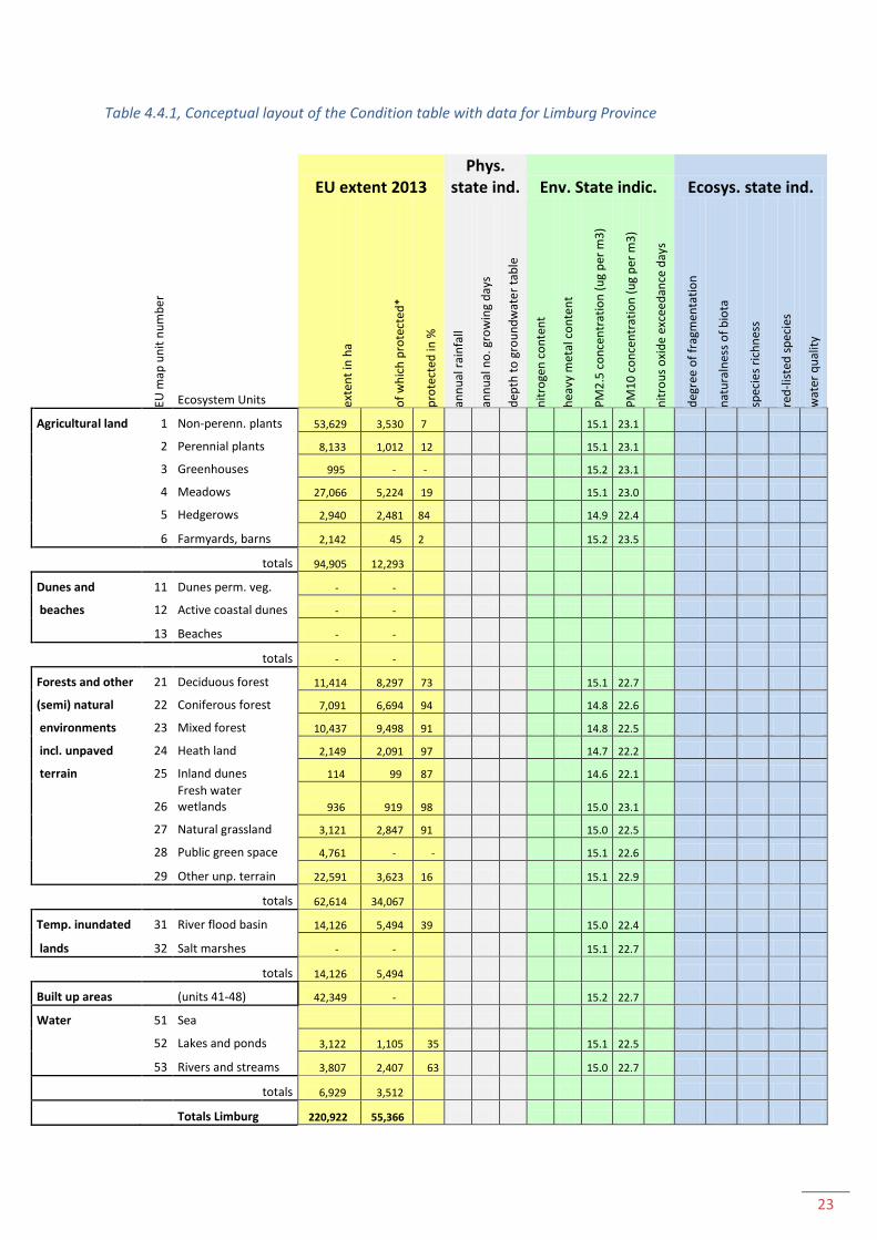
Table 4.4.1 shows the conceptual lay-out of a condition table representing data for a single year. If

more data, also within years, are available, the opening and closing values can be included for those

indicators for which this is relevant. First, the table shows information on ecosystem extent and

degree of protection. The table shows that the majority of forests, wetlands and heathlands in

Limburg are under a form of environmental protection. For the degree of protection the EU_NL map

was combined with the Natura2000 map. Therefore, the degree of protection varies within this

category, because national parks for example have a different degree of protection than areas that

are only part of the EHS. Such detailed information can also be made available depending upon

information needs of the users.

As described previously, condition indicators can be separated into physical, environmental state and

ecosystem state indicators. The table shows examples of a few possible indicators per category. The

physical state indicators contain data that describe the physical boundaries under which an

ecosystem is functioning. Examples are all climatic parameters (e.g. rainfall, wind regime,

temperature indicators etc.). In practical applications, this type of information would be shown in an

annex. For environmental state and ecosystem state indicators a few examples are provided. The

environmental state indicators reflect environmental, policy relevant indicators, but do not

necessarily reflect to the state of the ecosystem. For example, air pollution levels is an environmental

state indicator. It varies in time and in space, is highly policy-relevant, and is relevant for the

accounts because the higher the concentration of pollutants, in principle, the more air filtration

ecosystems can provide. The set of indicators can be extended in the future, depending on data

availability and the requirements of users.

As an example, annual mean particulate matter concentration values are also provided. The data

show that for this indicators the spatial differences are very small, which reflects the blanket cover of

PM in Limburg, with the highest concentrations in and near urban zones. The table also shows only

the background concentration of PM, not the local peak concentrations, which is the reason that

higher concentrations in urban zones do not show up in the Table. The example for PM is only

provided as an illustration, and more discussion with account users is needed to specify the condition

indicators and how they should be included in the account. The intention is to do this as part of the

process where the accounts would be scaled up.

23

Table 4.4.1, Conceptual layout of the Condition table with data for Limburg Province

EU extent 2013

Phys. state ind. Env. State indic. Ecosys. state ind.

EU m

ap u

nit

nu

mb

er

Ecosystem Units exte

nt

in h

a

of

wh

ich

pro

tect

ed*

pro

tect

ed in

%

ann

ual

rai

nfa

ll

ann

ual

no

. gro

win

g d

ays

dep

th t

o g

rou

nd

wat

er

tab

le

nit

roge

n c

on

ten

t

hea

vy m

etal

co

nte

nt

PM

2.5

co

nce

ntr

atio

n (

ug

per

m3

)

PM

10

co

nce

ntr

atio

n (

ug

per

m3

)

nit

rou

s o

xid

e ex

cee

dan

ce d

ays

deg

ree

of

frag

men

tati

on

nat

ura

lnes

s o

f b

iota

spec

ies

rich

nes

s

red

-lis

ted

sp

ecie

s

wat

er q

ual

ity

Agricultural land 1 Non-perenn. plants 53,629 3,530 7 15.1 23.1

2 Perennial plants 8,133 1,012 12 15.1 23.1

3 Greenhouses 995 - - 15.2 23.1

4 Meadows 27,066 5,224 19 15.1 23.0

5 Hedgerows 2,940 2,481 84 14.9 22.4

6 Farmyards, barns 2,142 45 2 15.2 23.5

totals 94,905 12,293

Dunes and 11 Dunes perm. veg. - -

beaches 12 Active coastal dunes - -

13 Beaches - -

totals - -

Forests and other 21 Deciduous forest 11,414 8,297 73 15.1 22.7

(semi) natural 22 Coniferous forest 7,091 6,694 94 14.8 22.6

environments 23 Mixed forest 10,437 9,498 91 14.8 22.5

incl. unpaved 24 Heath land 2,149 2,091 97 14.7 22.2

terrain 25 Inland dunes 114 99 87 14.6 22.1

26 Fresh water wetlands 936 919 98 15.0 23.1

27 Natural grassland 3,121 2,847 91 15.0 22.5

28 Public green space 4,761 - - 15.1 22.6

29 Other unp. terrain 22,591 3,623 16 15.1 22.9

totals 62,614 34,067

Temp. inundated 31 River flood basin 14,126 5,494 39 15.0 22.4

lands 32 Salt marshes - - 15.1 22.7

totals 14,126 5,494

Built up areas (units 41-48) 42,349 - 15.2 22.7

Water 51 Sea

52 Lakes and ponds 3,122 1,105 35 15.1 22.5

53 Rivers and streams 3,807 2,407 63 15.0 22.7

totals 6,929 3,512

Totals Limburg 220,922 55,366

24

5 Discussion and further recommendations

This pilot project has explored the possibilities of ecosystem accounting for a selected set of

ecosystem services in Limburg Province. The study illustrates the strong potential of the data that are

made available with the ecosystem accounting approach, following the SEEA – EEA guidelines.

However, the study also illustrates that a lot of work remains to be done; for Limburg several

economically and socially important ecosystem services were not yet included in the current pilot

project. Biophysical models are needed for a large number of additional ecosystem services, at a

level of detail that is sufficient to allow for both national scale accounting as well as small scale

(municipalities) comparisons. In addition, the quality of already existing biophysical supply models for

ecosystem services can be improved. Both tasks require collaboration with national institutes, in

particular (but not only) the ANK. Once completed for the Netherlands and for a broad set of

ecosystem services, the supply accounts provide information on the amount and location of supplied

ecosystem services. This gives insight in the wide range of services that are offered primarily by

natural and semi-natural vegetation, and it shows the locations of supply in detail. The spatial

information can be used to optimise the current use of ecosystem services, and to determine where

changes are most needed to protect or optimise ecosystem service supply. At the same time,

ecosystem condition indicators should be collected in a consistent manner. These sets of

information are vital to monitor the progress towards the goals set by the Dutch Government: to

achieve a sustainable use of ecosystem services and prevent further loss of biodiversity (Min.

Economic Affairs, 2013; Min. Economic Affairs et al., 2015). Protection of the natural environment is

highly important not just because of its (potentially incalculable) intrinsic value, but also because of

the services that provide clear economic benefits to businesses, governments and households.

To explore the full potential of ecosystem accounting, it is necessary to set up physical (and

monetary, see Report II) supply and use accounts at regular temporal intervals, where possible based

on the detailed EU_NL maps (also updated at the same temporal interval). The condition account is

essential to interpret spatial and temporal changes in the supply tables. The condition account also

provides information on ecologically and policy relevant ecosystem parameters. In addition to these

accounts, the SEEA-EEA guidelines propose the development of a number of accounts which would

provide information on the sustainability of ecosystem services supply and the monetary balance of

ecosystems. Ideally, such accounts would be developed at least at the national and provincial scale,

whereas ecosystem service supply maps and condition indicators provide meaningful information on

smaller scales as well.

The data on services supply and use for a single year, as presented in this study, help to identify

economic dependencies on ecosystem services and the location and relative importance of

contributors to ecosystem service supply. However, the main strength of the accounting approach

lies in the consistent, regular monitoring of ecosystem condition and services supply and use. Such

timeseries (which can be developed on national but also on smaller spatial scales) can be compared

to policy measures as well as economic and social developments.

25

Acknowledgements.

This pilot project was initiated in close collaboration with the ministries of Economic Affairs and

Infrastructure and the Environment. In particular we would like to thank the members of the steering

committee Henk Raven (Min. EZ), Wieger Dijkstra (Min. I en M), Saskia Ras (I en M), Joop van

Bodegraven (EZ) and Jan Hijkoop (BuZa) for their continued enthusiastic support and guidance. In

addition to the steering committee, comments and suggestions from the following persons were

greatly appreciated and helped to improve the final report as well as the focus of the study (all

members of the committee of external experts): Stefan van der Esch (PBL), Marcel Klok (Min EZ), Bart

de Knegt (WUR), Ton de Nijs (RIVM), Mattheüs van der Pol (Min EZ) and Arjan Ruijs (PBL). Marijn

Zuurmond (CBS) greatly contributed to the GIS work required in this study. Discussions with Chantal

Melser (CBS) and Ioulia Ossokinova (CPB) were greatly appreciated.

References

CBS, 2013. Environmental Accounts of the Netherlands, Chapter 7: Piloting Ecosystem Accounting. CBS, Den Haag/Heerlen IPCC, 2014. Climate Change 2014: Synthesis Report. Contribution of Working Groups I, II and III to the Fifth Assessment Report of the Intergovernmental Panel on Climate Change (Core Writing Team, R.K. Pachauri and L.A. Meyer (eds.)). IPCC, Geneva, Switzerland, 151 pp. Remme, R., Schröter, M., Hein, L., 2014. Developing spatial biophysical accounting for multiple ecosystem services. Ecosystem Services 10, p. 6 – 18. Remme, R., Edens, B., Schröter, M., Hein, L., 2015. Monetary accounting of ecosystem services: A test case for Limburg province, the Netherlands. Ecological Economics 112 (2015) 116–128 Secretariat of the Convention on Biological Diversity (2005). Handbook of the Convention on Biological Diversity Including its Cartagena Protocol on Biosafety, 3rd edition, (Montreal, Canada). TEEB, 2010. Mainstreaming the Economics of Nature: A Synthesis of the Approach, Conclusions and Recommendations of TEEB. UNEP-WCMC, 2015. Experimental Biodiversity Accounting as a component of the System of

Environmental-Economic Accounting Experimental Ecosystem Accounting (SEEA-EEA). Supporting

document to the Advancing the SEEA Experimental Ecosystem Accounting project. United Nations.

UN, EC, FAO, OECD, World Bank (2014), System of Environmental-Economic Accounting 2012. Experimental Ecosystem Accounting, United Nations, New York, USA

WCED (1987), Our Common Future: Report of the World Commission On Environment and Development. Oxford University, 1987.

26

Annex 1, EU_NL map for the Netherlands, 2013