Economics of the Firm Consumer Demand Analysis. Today’s Plan: Motivation Refresher on Probability...

Economics of the Firm

Consumer Demand Analysis

Today’s Plan:

•Motivation•Refresher on Probability and Statistics•Refresher on Regression analysis•Example of Regression Analysis•Cross Section Estimation •Forecasting•Questions

A demand curve tells us a lot about the customers that we face.

DVDMM PIPQ 264200

Movie Tickets Sold (in Thousands)

Price of a movie ticket

Average Income (in Thousands)

Price of a DVD (A substitute to the movies)

Every $1 increase in the price of a movie ticket lowers sales by 4,000 tickets

Every $1,000 increase in average income raises sales by 6,000 tickets

Every $1 increase in the price of a DVD raises sales by 2,000 tickets

DVDMM PIPQ 264200

We can use a demand curve to forecast sales and revenues…

12$

000,48$

8$

DVD

M

P

I

P

840,3$8$480

48012248684200

MM

M

QP

Q

Demand curves slope downwards – this reflects the negative relationship between price and quantity. Elasticity of Demand measures this effect quantitatively

Movie Tickets

Price

$8.00

480

D

Q

P

P

Q

P

QP %

%

DVDMM PIPQ 264200

067.480

84

MP

A 1% rise in price lowers sales by .067%

12$

000,48$

8$

DVD

M

P

I

P

For any fixed price, demand (typically) responds positively to increases in income. Income Elasticity measures this effect quantitatively

Movie Tickets

Price

$8.00

480

D

Q

I

I

Q

I

QI %

%

'D

6.480

486

I

A 1% rise in average income raises sales by .6%

DVDMM PIPQ 264200

12$

000,48$

8$

DVD

M

P

I

P

Cross price elasticity refers to the impact on demand of another price changing

Movie Tickets

Price

$4.00

480

D

Q

P

P

Q

P

Q DVD

DVDDVDL %

%

'D

A positive cross price elasticity refers to a substitute while a negative cross price elasticity refers to a compliment

DVDMM PIPQ 264200

12$

000,48$

8$

DVD

M

P

I

P

05.480

122

DVDP

A 1% rise in DVD prices raises sales by .05%

Application: At the revenue maximizing price, elasticity should be -1

DVDMM PIPQ 264200

12$

000,48$

DVDP

I

MM PQ 4512

14512

4

M

MP P

PM

384,16$

256

64$

MM

M

QP

Q

P

We can then re-calculate elasticity

DVDMM PIPQ 264200

12$

000,48$

64$

DVD

M

P

I

P

256MQ

1256

644

MP 125.1

256

486

I 09.

256

122

DVDP

A 1% rise in price lowers sales by 1%

A 1% rise in average income raises sales by 1.125%

A 1% rise in DVD prices raises sales by .09%

Suppose that average income rose by 8%. By how much could you raise price without losing any sales?

DVDPIMPM PIPQDVDM

%%%%

09.

125.1

1

DVD

M

P

I

P

0009.825.1%% MM PQ

10% MP

All We need is a demand curve!!

What are the odds that a fair coin flip results in a head?

What are the odds that the toss of a fair die results in a 5?

What are the odds that tomorrow’s temperature is 95 degrees?

http://images.google.com/imgres?imgurl=http://www.coinfacts.com/quarter_dollars/50_states_quarters/50_states_quarter_obv_large.jpg&imgrefurl=http://www.coinfacts.com/quarter_dollars/50_states_quarters/50_states_quarters.htm&usg=__aJcCaQUJVBDMLNrsrguN0Rv8hOQ=&h=330&w=332&sz=58&hl=en&start=1&um=1&tbnid=qv2Z5v0xoJtvsM:&tbnh=118&tbnw=119&prev=/images?q=quarter&hl=en&rls=com.microsoft:*&sa=N&um=1

http://images.google.com/imgres?imgurl=http://farm3.static.flickr.com/2389/1974871417_11d5c49ac3.jpg&imgrefurl=http://www.flickr.com/photos/powerhouse_museum_photography/1974871417/&usg=__UAIANNaIL-2mLgptyj0ZBGpSv0k=&h=337&w=425&sz=34&hl=en&start=24&um=1&tbnid=FEPyU6gdCqhFpM:&tbnh=100&tbnw=126&prev=/images?q=dice&ndsp=21&hl=en&rls=com.microsoft:*&sa=N&start=21&um=1

http://images.google.com/imgres?imgurl=http://www.afc.rutgers.edu/images/SummerSun.gif&imgrefurl=http://www.afc.rutgers.edu/&usg=__vw3C5oZZm_PB5u9odkslYRU9fOg=&h=340&w=392&sz=5&hl=en&start=4&um=1&tbnid=qO4aJ-O4WBwIbM:&tbnh=107&tbnw=123&prev=/images?q=summer&hl=en&rls=com.microsoft:*&um=1

The answer to all these questions come from a probability distribution

Head Tail

1/2

Probability

1 6

1/6

Probability

2 3 4 5

A probability distribution is a collection of probabilities describing the odds of any particular event


http://images.google.com/imgres?imgurl=http://farm3.static.flickr.com/2389/1974871417_11d5c49ac3.jpg&imgrefurl=http://www.flickr.com/photos/powerhouse_museum_photography/1974871417/&usg=__UAIANNaIL-2mLgptyj0ZBGpSv0k=&h=337&w=425&sz=34&hl=en&start=24&um=1&tbnid=FEPyU6gdCqhFpM:&tbnh=100&tbnw=126&prev=/images?q=dice&ndsp=21&hl=en&rls=com.microsoft:*&sa=N&start=21&um=1

Probability

TemperatureMean Mean+1SD Mean+2SDMean -1SDMean-2SD

2.5% 2.5%13.5% 34% 34% 13.5%

We generally assume a Normal Distribution which can be characterized by a mean (average) and standard deviation (measure of dispersion)

Annual Temperature in South Bend has a mean of 59 degrees and a standard deviation of 18 degrees.

Probability

Temperature59 77 954123

95 degrees is 2 standard deviations to the right – there is a 2.5% chance the temperature is 95 or greater (97.5% chance it is cooler than 95)

Can’t we do a little better than this?

Conditional distributions give us probabilities conditional on some observable information – the temperature in South Bend conditional on the month of July has a mean of 84 with a standard deviation of 7.

Probability

Temperature84 91 987770

95 degrees falls a little more than one standard deviation away (there approximately a 16% chance that the temperature is 95 or greater)

95

Conditioning on month gives us a more accurate probabilities!

5.PrPr TailsHeads

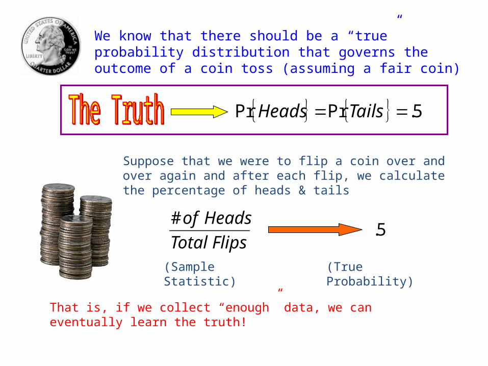
We know that there should be a “true” probability distribution that governs the outcome of a coin toss (assuming a fair coin)

Suppose that we were to flip a coin over and over again and after each flip, we calculate the percentage of heads & tails

FlipsTotal

Headsof

#5.

That is, if we collect “enough” data, we can eventually learn the truth!

(Sample Statistic) (True Probability)


We can follow the same process for the temperature in South Bend

Temperature ~ 2,N

We could find this distribution by collecting temperature data for south bend

N

iixN

x1

1

2

1

22 1

N

ii xx

Ns

Sample Mean

(Average)

Sample Variance

Note: Standard Deviation is the square root of the variance.

Mean = 8

Std. Dev. = 2

Mean = $ 12,000

Std. Dev. = $ 2,000

Suppose we know that the value of a car is determined by its age

Value = $20,000 - $1,000 (Age)

Car Age Value

We could also use this to forecast:

Value = $20,000 - $1,000 (Age)

How much should a six year old car be worth?

Value = $20,000 - $1,000 (6) = $14,000

Note: There is NO uncertainty in this prediction.

Value = a + b * (Age) + error 20,σNerror

We want to choose ‘a’ and ‘b’ to minimize the error!

a

Slope = b

Searching for the truth….a linear regression

Error

Error

Regression Results

Variable Coefficients Standard Error t Stat

Intercept 12,354 653 18.9

Age - 854 80 -10.60

Value = $12,354 - $854 * (Age) + error

We have our estimate of “the truth”

Intercept (a)

Mean = $12,354

Std. Dev. = $653

Age (b)

Mean = -$854

Std. Dev. = $80

T-Stats bigger than 2 in absolute value are considered statistically significant!

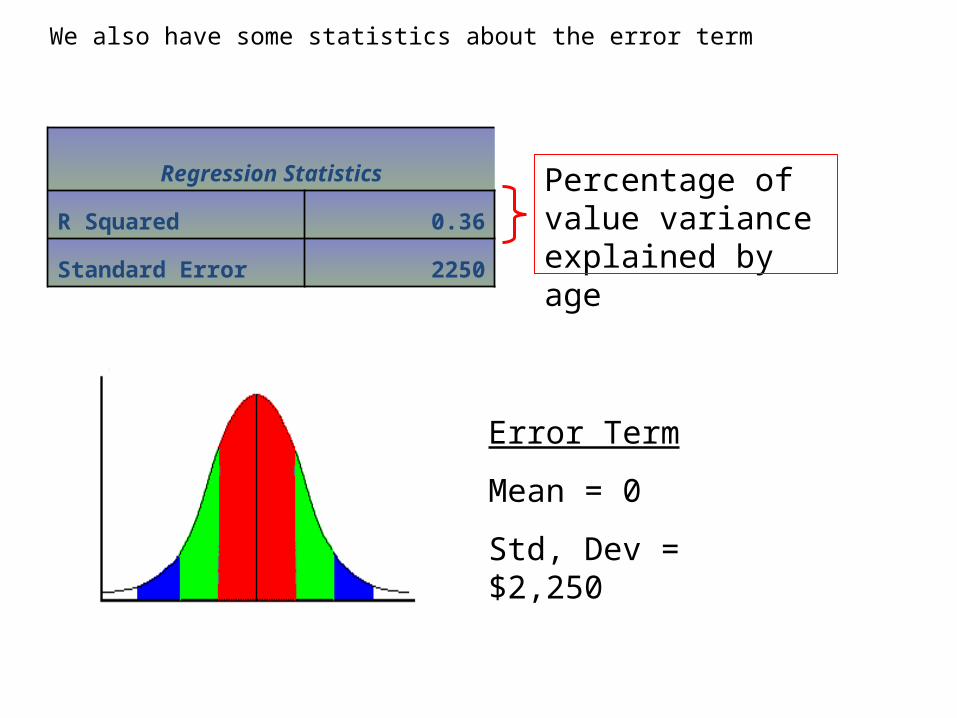
Regression Statistics

R Squared 0.36

Standard Error 2250

Error Term

Mean = 0

Std, Dev = $2,250

Percentage of value variance explained by age

We also have some statistics about the error term

We can now forecast the value of a 6 year old car

Salary = $12,354 - $854 * (Age) + error

6

Mean = $12,354

Std. Dev. = $653

Mean = $854

Std. Dev. = $ 80

Mean = $0

Std. Dev. = $2,250

errorVarbVarXbVarXaVarStdDev 22

(Recall, The Average Car age is 8 years)

259,2$225080862806653 22222 StdDev

230,7$6*854354,12 Value

8x

+95%

-95%

Age

Value

Note that your forecast error will always be smallest at the sample mean! Also, your forecast gets worse at an increasing rate as you depart from the mean

6Age

Forecast Interval

259,2$225080862806653 22222 StdDev

230,7$6*854354,12 Value

What are the odds that Pat Buchanan received 3,407 votes from Palm Beach County in 2000?

An applied example…

The Strategy: Estimate a relationship for Pat Buchanan’s votes using every county EXCEPT Palm Beach Using Palm Beach data,

forecast Pat Buchanan’s vote total for Palm Beach

DFB

Pat Buchanan’s Votes

“Are a function of”

Observable Demographics

PBPB DFB

The Data: Demographic Data By County

County Black (%)

Age 65 (%)

Hispanic (%)

College (%)

Income (000s)

Buchanan Votes

Total Votes

Alachua 21.8 9.4 4.7 34.6 26.5 262 84,966

Baker 16.8 7.7 1.5 5.7 27.6 73 8,128

What variables do you think should affect Pat Buchanan’s Vote total?

bCaV

% of County that is college educated

# of votes gained/lost for each percentage point increase in college educated population

# of Buchanan votes

Parameter a b

Value 5.35 14.95

Standard Error 58.5 3.84

T-Statistic .09 3.89

Results R-Square = .19

CV 95.1435.5

The distribution for ‘b’ has a mean of 15 and a standard deviation of 4

15

There is a 95% chance that the value for ‘b’ lies between 23 and 7

County College (%)

Predicted Votes

Actual Votes

Error

Alachua 34.6 522 262 260

Baker 5.7 90 73 17

0

Plug in Values for College % to get vote predictions

19% of the variation in Buchanan’s votes across counties is explained by college education

Each percentage point increase in college educated (i.e. from 10% to 11%) raises Buchanan’s vote total by 15

County College (%) Buchanan Votes

Log of Buchanan Votes

Alachua 34.6 262 5.57

Baker 5.7 73 4.29

Lets try something a little different…

bCaVLN

% of County that is college educated

Percentage increase/decease in votes for each percentage point increase in college educated population

Log of Buchanan votes

Parameter a b

Value 3.45 .09

Standard Error .27 .02

T-Statistic 12.6 5.4


CVLN 09.45.3

The distribution for ‘b’ has a mean of .09 and a standard deviation of .02

.09

There is a 95% chance that the value for ‘b’ lies between .13 and .05

County College (%)

Predicted Votes

Actual Votes

Error

Alachua 34.6 902 262 640

Baker 5.7 55 73 -18

0



VLNeV

Each percentage point increase in college educated (i.e. from 10% to 11%) raises Buchanan’s vote total by .09%

County College (%) Buchanan Votes

Log of College (%)

Alachua 34.6 262 3.54

Baker 5.7 73 1.74

How about this…

CbLNaV

Log of % of County that is college educated

Gain/ Loss in votes for each percentage increase in college educated population

# of Buchanan votes

Parameter a b

Value -424 252

Standard Error 139 54

T-Statistic -3.05 4.6


CLNV 252424

The distribution for ‘b’ has a mean of 252 and a standard deviation of 54

.09

There is a 95% chance that the value for ‘b’ lies between 360 and 144

County College (%)

Predicted Votes

Actual Votes

Error

Alachua 34.6 469 262 207

Baker 5.7 15 73 -58

0



Each percentage increase in college educated (i.e. from 30% to 30.3%) raises Buchanan’s vote total by 252 votes

County College (%)

Buchanan Votes

Log of College (%) Log of Buchanan Votes

Alachua 34.6 262 3.54 5.57

Baker 5.7 73 1.74 4.29

One More…

CbLNaVLN

Log of % of County that is college educated

Percentage gain/Loss in votes for each percentage increase in college educated population

Log of Buchanan votes

Parameter a b

Value .71 1.61

Standard Error .63 .24

T-Statistic 1.13 6.53


CLNVLN 61.171.

The distribution for ‘b’ has a mean of 1.61 and a standard deviation of .24

.09

There is a 95% chance that the value for ‘b’ lies between 2 and 1.13

County College (%)

Predicted Votes

Actual Votes

Error

Alachua 34.6 624 262 362

Baker 5.7 34 73 -39

0



Each percentage increase in college educated (i.e. from 30% to 30.3%) raises Buchanan’s vote total by 1.61%

VLNeV

It turns out the regression with the best fit looks like this.

County Black (%)

Age 65 (%)

Hispanic (%)

College (%)

Income (000s)

Buchanan Votes

Total Votes

Alachua 21.8 9.4 4.7 34.6 26.5 262 84,966

Baker 16.8 7.7 1.5 5.7 27.6 73 8,128

IaCaHaAaBaaPLN 54365221

Parameters to be estimated

Error termBuchanan Votes

Total Votes*100

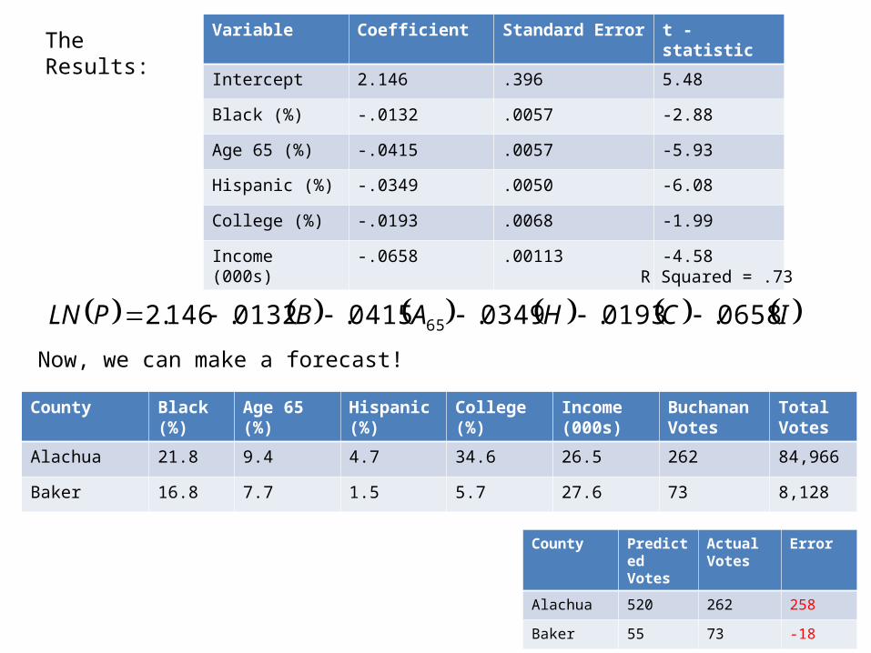
The Results: Variable Coefficient Standard Error t - statistic

Intercept 2.146 .396 5.48

Black (%) -.0132 .0057 -2.88

Age 65 (%) -.0415 .0057 -5.93

Hispanic (%) -.0349 .0050 -6.08

College (%) -.0193 .0068 -1.99

Income (000s) -.0658 .00113 -4.58

Now, we can make a forecast!

ICHABPLN 0658.0193.0349.0415.0132.146.2 65

R Squared = .73

County Predicted Votes

Actual Votes

Error

Alachua 520 262 258

Baker 55 73 -18

County Black (%) Age 65 (%) Hispanic (%) College (%) Income (000s)

Buchanan Votes

Total Votes

Alachua 21.8 9.4 4.7 34.6 26.5 262 84,966

Baker 16.8 7.7 1.5 5.7 27.6 73 8,128

County Black (%)

Age 65 (%)

Hispanic (%)

College (%)

Income (000s)

Buchanan Votes

Total Votes

Palm Beach 21.8 23.6 9.8 22.1 33.5 3,407 431,621

004.2PLN

%134.004.2 eP

578621,43100134. This would be our prediction for Pat Buchanan’s vote total!

ICHABPLN 0658.0193.0349.0415.0132.146.2 65

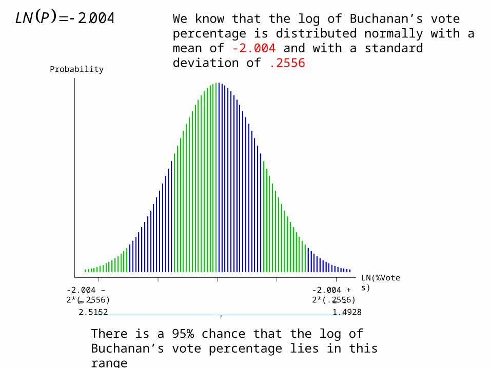
Probability

LN(%Votes)

There is a 95% chance that the log of Buchanan’s vote percentage lies in this range

-2.004 – 2*(.2556) -2.004 + 2*(.2556)= -2.5152 = -1.4928

004.2PLN We know that the log of Buchanan’s vote percentage is distributed normally with a mean of -2.004 and with a standard deviation of .2556

Probability

% of Votes

There is a 95% chance that Buchanan’s vote percentage lies in this range

%134.004.2 eP

%08.5152.2 e %22.4928.1 e

Next, lets convert the Logs to vote percentages

Probability

Votes

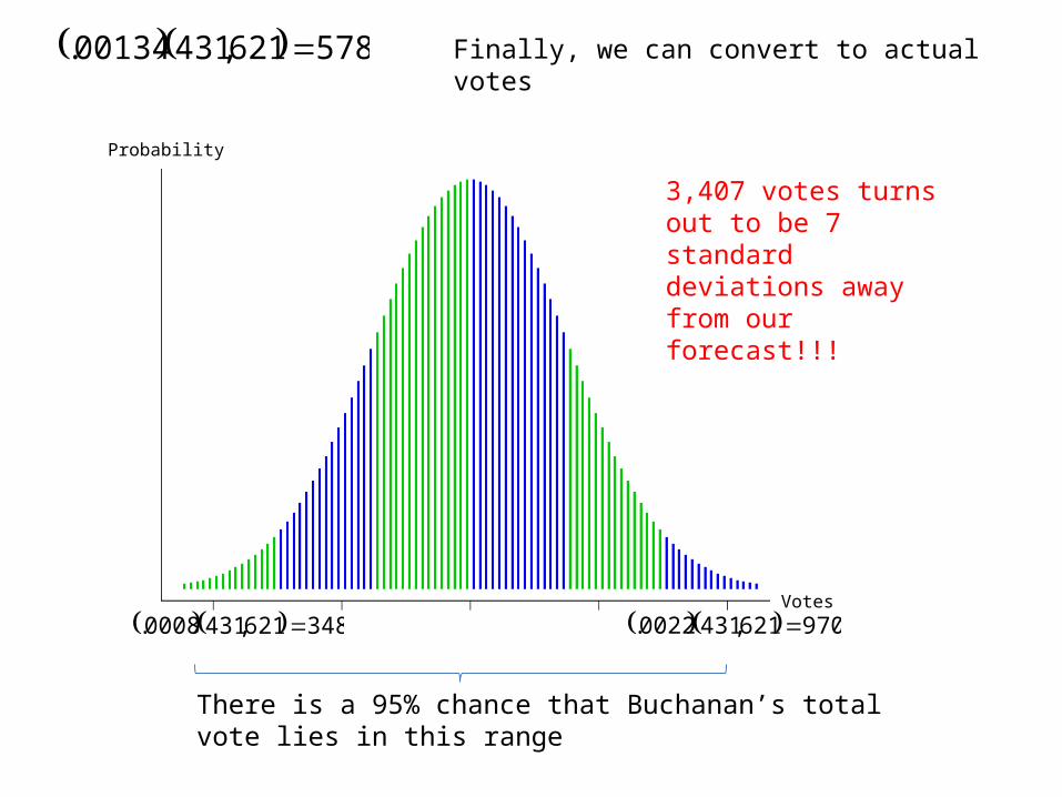
There is a 95% chance that Buchanan’s total vote lies in this range

348621,4310008. 970621,4310022.

Finally, we can convert to actual votes 578621,43100134.

3,407 votes turns out to be 7 standard deviations away from our forecast!!!

Back to the original problem. We know that the quantity of some good or service demanded should be related to some basic variables

Quantity

Price

D

,..., IPDQD

Quantity Demanded Price

Income

Other “Demand Shifters”

“ Is a function of”

Time

Dem

and

Fact

ors

t t+1t-1

Cross Sectional estimation holds the time period constant and estimates the variation in demand resulting from variation in the demand factors

For example: can we estimate demand for Pepsi in South Bend by looking at selected statistics for South bend

City Price Average Income (Thousands)

Competitor’s Price

Advertising Expenditures (Thousands)

Total Sales

Granger 1.02 21.934 1.48 2.367 9,809

Mishawaka 2.56 35.796 2.53 26.922 130,835

Suppose that we have the following data for sales in 200 different Indiana cities

Lets begin by estimating a basic demand curve – quantity demanded is a linear function of price.

PaaQ 10

Change in quantity demanded per $ change in price (to be estimated)

Regression Results

Variable Coefficient Standard Error t Stat

Intercept 155,042 18,133 8.55

Price (X) -46,087 7214 -6.39

PQ 087,46042,155

That is, we have estimated the following equation


R Squared .17

Standard Error 48,074

Every dollar increase in price lowers sales by 46,087 units.

Values For South BendPrice of Pepsi $1.37

903,9137.1087,46042,155 Q

P

Q

$1.37

91,903

We can now use this estimated demand curve along with price in South Bend to estimate demand in South Bend

903,91

37.1087,46

087,46

Q

p

p

Q

p

Q

903,9137.1087,46042,155

37.1$

Q

P

68.903,91

37.1087,46

P

Q91,903

$1.37

We can get a better sense of magnitude if we convert the estimated coefficient to an elasticity

PQ 087,46042,155




Total Sales

Granger 1.02 21.934 1.48 2.367 9,809

Mishawaka 2.56 35.796 2.53 26.922 130,835

As we did earlier, we can experiment with different functional forms by using logs

Using logs changes the interpretation of the coefficients.

PLNaaQ 10

Change in quantity demanded per percentage change in price (to be estimated)

Regression Results


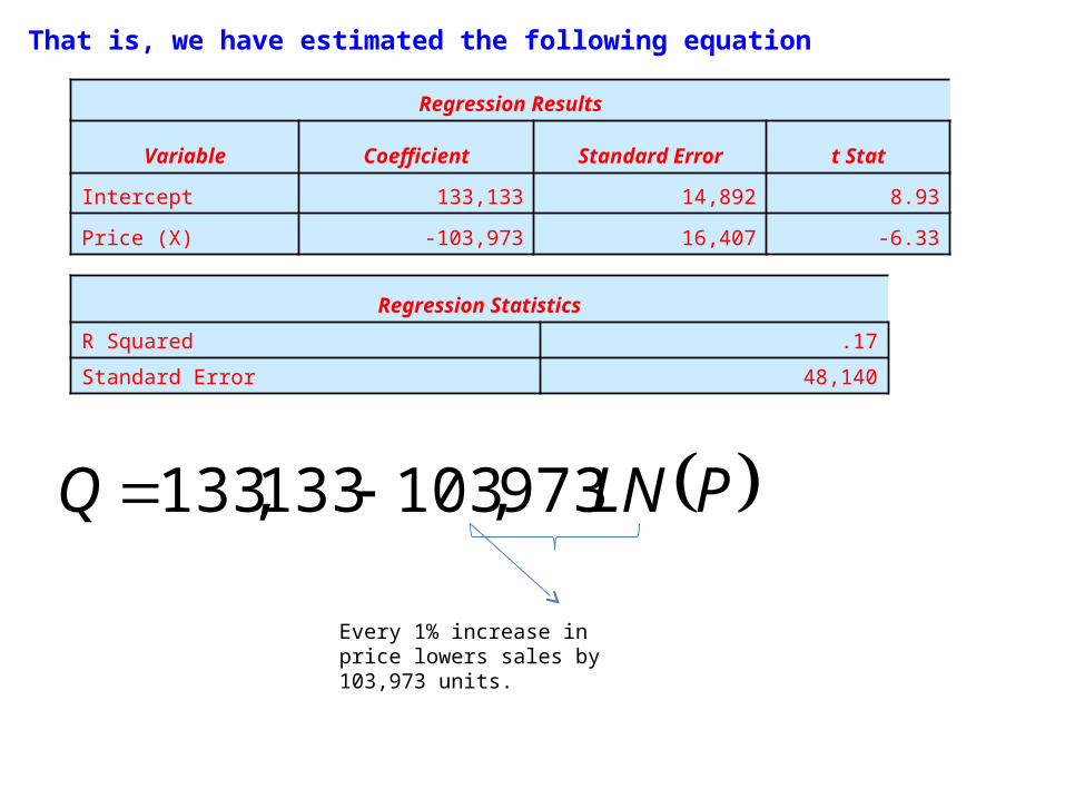
Intercept 133,133 14,892 8.93

Price (X) -103,973 16,407 -6.33

PLNQ 973,103133,133



R Squared .17

Standard Error 48,140

Every 1% increase in price lowers sales by 103,973 units.


Log of Price .31

P

Q

$1.37

100,402


31.973,103133,133 Q


PQ 973,103133,133

P

Q

$1.37

100,402

402,100

1973,103

1

973,103%

Qp

Q

p

Q

402,10031973,103133,133

31.37.1

Q

LNPLN

04.1402,100

1973,103




Total Sales

Granger 1.02 21.934 1.48 2.367 9,809

Mishawaka 2.56 35.796 2.53 26.922 130,835


PaaQLN 10

Percentage change in quantity demanded per $ change in price (to be estimated)


Regression Results


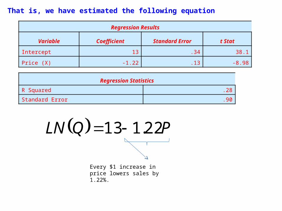
Intercept 13 .34 38.1

Price (X) -1.22 .13 -8.98

PQLN 22.113



R Squared .28

Standard Error .90

Every $1 increase in price lowers sales by 1.22%.


P

Q

$1.37

83,283


283,83

33.1137.122.11333.11

eQ

QLN


P

Q

$1.37

83,283

1

37.122.1

1

%

22.1%

p

p

Q

p

Q

67.1

1

37.122.1

PQLN 22.113

283,83

33.1137.122.11333.11

eQ

QLN




Total Sales

Granger 1.02 21.934 1.48 2.367 9,809

Mishawaka 2.56 35.796 2.53 26.922 130,835


PLNaaQLN 10

Percentage change in quantity demanded per percentage change in price (to be estimated)


Regression Results


Intercept 12.3 .28 42.9

Price (X) -2.60 .31 -8.21

PLNQLN 6.212



R Squared .25

Standard Error .93

Every 1% increase in price lowers sales by 2.6%.


Log of Price .31

P

Q

$1.37

72,402


402,72

19.1131.6.21219.11

eQ

QLN


P

Q

$1.37

83,283

6.2%

%

p

Q

6.2

PLNQLN 6.212

402,72

19.1131.6.21219.11

eQ

QLN

We can add as many variables as we want in whatever combination. The goal is to look for the best fit.

cPLNaILNaPaaQLN 3210

% change in Sales per $ change in price

% change in Sales per % change in income

% change in Sales per % change in competitor’s price

Regression Results


Intercept 5.98 1.29 4.63

Price -1.29 .12 -10.79

Log of Income 1.46 .34 4.29

Log of Competitor’s Price 2.00 .34 5.80

R Squared: .46


Log of Income 3.81

Log of Competitor’s Price .80

P

Q

$1.37

87,142

142,87

36.1180.00.281.346.137.129.198.536.11

eQ

QLN

Now we can make a prediction and calculate elasticities

00.2%

%

46.1%

%

76.11

37.129.1

1

%

cCP

I

P

Q

I

Q

P

P

Q

Time

Dem

and

Fact

ors

t t+1t-1

We could use a cross sectional regression to forecast quantity demanded out into the future, but it would take a lot of information!

Estimate a demand curve using data at some point in time

Use the estimated demand curve and forecasts of data to forecast quantity demanded

Time

Dem

and

Fact

ors

t t+1t-1

Time Series estimation ignores the demand factors constant and estimates the variation in demand over time

For example: can we predict demand for Pepsi in South Bend next year by looking at how demand varies across time

Time series estimation leaves the demand factors constant and looks at variations in demand over time. Essentially, we want to separate demand changes into various frequencies

Trend: Long term movements in demand (i.e. demand for movie tickets grows by an average of 6% per year)

Business Cycle: Movements in demand related to the state of the economy (i.e. demand for movie tickets grows by more than 6% during economic expansions and less than 6% during recessions)

Seasonal: Movements in demand related to time of year. (i.e. demand for movie tickets is highest in the summer and around Christmas

Suppose that you work for a local power company. You have been asked to forecast energy demand for the upcoming year. You have data over the previous 4 years:

Time Period Quantity (millions of kilowatt hours)

2003:1 11

2003:2 15

2003:3 12

2003:4 14

2004:1 12

2004:2 17

2004:3 13

2004:4 16

2005:1 14

2005:2 18

2005:3 15

2005:4 17

2006:1 15

2006:2 20

2006:3 16

2006:4 19

0

5

10

15

20

25

2003-1 2004-1 2005-1 2006-1

First, let’s plot the data…what do you see?

This data seems to have a linear trend

A linear trend takes the following form:

btxxt 0

Forecasted value at time t (note: time periods are quarters and time zero is 2003:1)

Time period: t = 0 is 2003:1 and periods are quarters

Estimated value for time zero

Estimated quarterly growth (in kilowatt hours)

Regression Results


Intercept 11.9 .953 12.5

Time Trend .394 .099 4.00


R Squared .53

Standard Error 1.82

Observations 16txt 394.9.11

Lets forecast electricity usage at the mean time period (t = 8)

50.3ˆ

05.158394.9.11ˆ

t

t

xVar

x

0

5

10

15

20

25

2003-1 2004-1 2005-1 2006-1

Here’s a plot of our regression line with our error bands…again, note that the forecast error will be lowest at the mean time period

T = 8

0

10

20

30

40

50

60

70

Sample

We can use this linear trend model to predict as far out as we want, but note that the error involved gets worse!

7.47ˆ

85.4176394.9.11ˆ

t

t

xVar

x

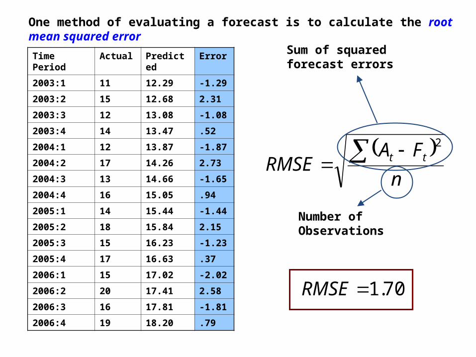
Time Period Actual Predicted Error

2003:1 11 12.29 -1.29

2003:2 15 12.68 2.31

2003:3 12 13.08 -1.08

2003:4 14 13.47 .52

2004:1 12 13.87 -1.87

2004:2 17 14.26 2.73

2004:3 13 14.66 -1.65

2004:4 16 15.05 .94

2005:1 14 15.44 -1.44

2005:2 18 15.84 2.15

2005:3 15 16.23 -1.23

2005:4 17 16.63 .37

2006:1 15 17.02 -2.02

2006:2 20 17.41 2.58

2006:3 16 17.81 -1.81

2006:4 19 18.20 .79

One method of evaluating a forecast is to calculate the root mean squared error

n

FARMSE tt

2

Number of Observations

Sum of squared forecast errors

70.1RMSE

0

5

10

15

20

25

2003-1 2004-1 2005-1 2006-1

Lets take another look at the data…it seems that there is a regular pattern…

Q2

Q2Q2

Q2

We are systematically under predicting usage in the second quarter

Time Period Actual Predicted Ratio Adjusted

2003:1 11 12.29 .89 12.29(.87)=10.90

2003:2 15 12.68 1.18 12.68(1.16) = 14.77

2003:3 12 13.08 .91 13.08(.91) = 11.86

2003:4 14 13.47 1.03 13.47(1.04) = 14.04

2004:1 12 13.87 .87 13.87(.87) = 12.30

2004:2 17 14.26 1.19 14.26(1.16) = 16.61

2004:3 13 14.66 .88 14.66(.91) = 13.29

2004:4 16 15.05 1.06 15.05(1.04) = 15.68

2005:1 14 15.44 .91 15.44(.87) = 13.70

2005:2 18 15.84 1.14 15.84(1.16) = 18.45

2005:3 15 16.23 .92 16.23(.91) = 14.72

2005:4 17 16.63 1.02 16.63(1.04) = 17.33

2006:1 15 17.02 .88 17.02(.87) = 15.10

2006:2 20 17.41 1.14 17.41(1.16) = 20.28

2006:3 16 17.81 .89 17.81(.91) = 16.15

2006:4 19 18.20 1.04 18.20(1.04) = 18.96

Average Ratios

•Q1 = .87

•Q2 = 1.16

•Q3 = .91

•Q4 = 1.04

We can adjust for this seasonal component…

10

11

12

13

14

15

16

17

18

19

20

2003-1 2004-1 2005-1 2006-1

Now, we have a pretty good fit!!

26.RMSE

0

10

20

30

40

50

60

70

52.4304.185.4176394.9.11ˆ tx

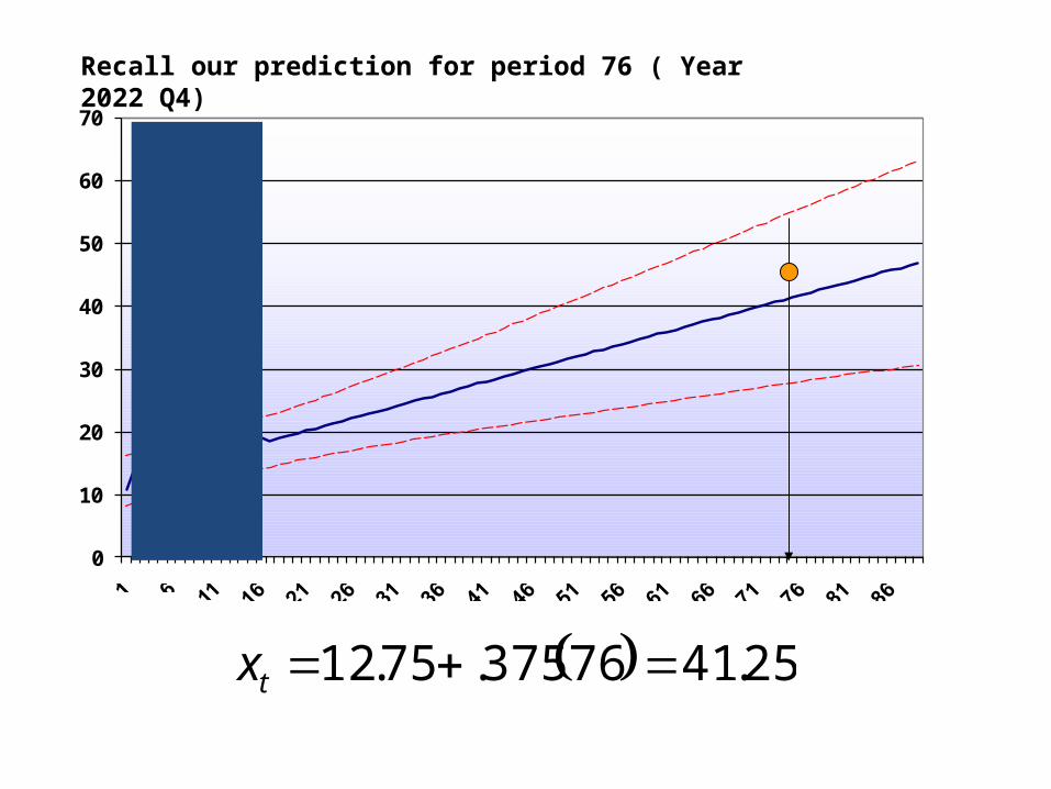
Recall our prediction for period 76 ( Year 2022 Q4)

We could also account for seasonal variation by using dummy variables

33221100 DbDbDbtbxxt

else

iquarterifDi ,0

,1

Note: we only need three quarter dummies. If the observation is from quarter 4, then

tbxx

DDD

t 00

321 0

Regression Results


Intercept 12.75 .226 56.38

Time Trend .375 .0168 22.2

D1 -2.375 .219 -10.83

D2 1.75 .215 8.1

D3 -2.125 .213 -9.93


R Squared .99

Standard Error .30

Observations 16

321 125.275.1375.2375.75.12 DDDtxt

Note the much better fit!!

Time Period Actual Ratio Method Dummy Variables

2003:1 11 10.90 10.75

2003:2 15 14.77 15.25

2003:3 12 11.86 11.75

2003:4 14 14.04 14.25

2004:1 12 12.30 12.25

2004:2 17 16.61 16.75

2004:3 13 13.29 13.25

2004:4 16 15.68 15.75

2005:1 14 13.70 13.75

2005:2 18 18.45 18.25

2005:3 15 14.72 14.75

2005:4 17 17.33 17.25

2006:1 15 15.10 15.25

2006:2 20 20.28 19.75

2006:3 16 16.15 16.25

2006:4 19 18.96 18.75

26.RMSE

Ratio Method

25.RMSE

Dummy Variables

0

10

20

30

40

50

60

70

Recall our prediction for period 76 ( Year 2022 Q4)

25.4176375.75.12 tx

btxxt 0

Recall, our trend line took the form…

This parameter is measuring quarterly change in electricity demand in millions of kilowatt hours.

Often times, its more realistic to assume that demand grows by a constant percentage rather that a constant quantity. For example, if we knew that electricity demand grew by g% per quarter, then our forecasting equation would take the form

t

t

gxx

100

%10

tt gxx 10

If we wish to estimate this equation, we have a little work to do…

Note: this growth rate is in decimal form

gtxxt 1lnlnln 0

If we convert our data to natural logs, we get the following linear relationship that can be estimated

Regression Results


Intercept 2.49 .063 39.6

Time Trend .026 .006 4.06


R Squared .54

Standard Error .1197

Observations 16

txt 026.49.2ln

Lets forecast electricity usage at the mean time period (t = 8)

0152.ˆ

698.28026.49.2ˆln

t

t

xVar

xBE CAREFUL….THESE NUMBERS ARE LOGS !!!

0152.ˆ

698.28026.49.2ˆln

t

t

xVar

x

The natural log of forecasted demand is 2.698. Therefore, to get the actual demand forecast, use the exponential function

85.14698.2 e

Likewise, with the error bands…a 95% confidence interval is +/- 2 SD

945.2,451.20152.2/698.2

00.19,60.11, 945.2451.2 ee

0

5

10

15

20

25

30

2003-1 2004-1 2005-1 2006-1

Again, here is a plot of our forecasts with the error bands

T = 8 70.1RMSE

0

100

200

300

400

500

600

1 13 25 37 49 61 73 85 97

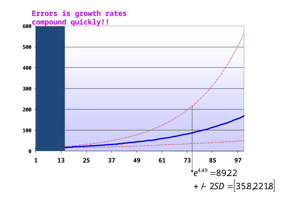
8.221,8.352/

22.8949.4

SD

e

Errors is growth rates compound quickly!!

Let’s try one…suppose that we are interested in forecasting gasoline prices. We have the following historical data. (the data is monthly from April 1993 – June 2010)

Does a linear (constant cents per gallon growth per year) look reasonable?

Let’s suppose we assume a linear trend. Then we are estimating the following linear regression:

btppt 0

Price at time t Price at April 1993 Number of months from April 1993

monthly growth in cents per gallon

Regression Results


Intercept .67 .05 12.19

Time Trend .010 .0004 23.19

R Squared= .72

We can check for the presence of a seasonal cycle by adding seasonal dummy variables:

33221100 DbDbDbtbppt

else

iquarterifDi ,0

,1

Cents per gallon impact of quarter I relative to quarter 4

Regression Results


Intercept .58 .07 8.28

Time Trend .01 .0004 23.7

D1 -.03 .075 -.43

D2 .15 .074 2.06

D3 .16 .075 2.20

R Squared= .74

If we wanted to remove the seasonal component, we could by subtracting the seasonal dummy off each gas price

Seasonalizing

Date PriceRegression

coefficientSeasonalized

data

1993 – 04 1.05 .15 .90

1993 - 07 1.06 .16 90

1993 - 10 1.06 0 1.06

1994 - 01 .98 -.03 1.01

1994 - 04 1.00 .15 .85

2nd Quarter

3rd Quarter

4th Quarter

1st Quarter

2nd Quarter

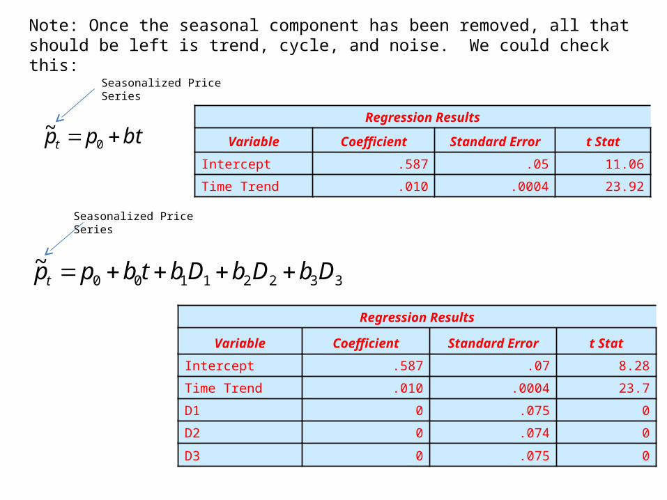
Note: Once the seasonal component has been removed, all that should be left is trend, cycle, and noise. We could check this:

btppt 0~

Seasonalized Price Series

Regression Results


Intercept .587 .05 11.06

Time Trend .010 .0004 23.92

33221100~ DbDbDbtbppt

Seasonalized Price Series

Regression Results


Intercept .587 .07 8.28

Time Trend .010 .0004 23.7

D1 0 .075 0

D2 0 .074 0

D3 0 .075 0

321 16.15.03.01.58. DDDtpt

The regression we have in place gives us the trend plus the seasonal component of the data

Trend Seasonal

If we subtract our predicted price (from the regression) from the actual price, we will have isolated the business cycle and noise

Business Cycle Component

Date Actual Price

Predicted Price (From

regression)Business Cycle

Component

1993 - 04 1.050 .752 .297

1993 - 05 1.071 .763 .308

1993 - 06 1.075 773 .301

1993 - 07 1.064 .797 .267

1993 - 08 1.048 .807 .240

Predicted

We can plot this and compare it with business cycle dates

tt pp ˆActual Price

Predicted Price

Data Breakdown

Date Actual Price Trend Seasonal Business Cycle

1993 - 04 1.050 .60 .15 .30

1993 - 05 1.071 .61 .15 .31

1993 - 06 1.075 .62 .15 .30

1993 - 07 1.064 .63 .16 .27

1993 - 08 1.048 .64 .16 .24

Regression Results


Intercept .58 .07 8.28

Time Trend .01 .0004 23.7

D1 -.03 .075 -.43

D2 .15 .074 2.06

D3 .16 .075 2.20

Perhaps an exponential trend would work better…

An exponential trend would indicate constant percentage growth rather than cents per gallon.

We already know that there is a seasonal component, so we can start with dummy variables

33221100ln DbDbDbtbppt

else

iquarterifDi ,0

,1

Percentage price impact of quarter I relative to quarter 4

Regression Results


Intercept -.14 .03 -4.64

Time Trend .005 .0001 29.9

D1 -.02 .032 -.59

D2 .06 .032 2.07

D3 .07 .032 2.19

R Squared= .81

Monthly growth rate

If we wanted to remove the seasonal component, we could by subtracting the seasonal dummy off each gas price, but now, the price is in logs

Seasonalizing

Date Price Log of PriceRegression

coefficientLog of Seasonalized

dataSeasonalized

Price

1993 – 04 1.05 .049 .06 -.019 .98

1993 - 07 1.06 .062 .07 -.010 .99

1993 - 10 1.06 .062 0 .062 1.06

1994 - 01 .98 -.013 -.02 .006 1.00

1994 - 04 1.00 .005 .06 -.062 .94

2nd Quarter

3rd Quarter

4th Quarter

1st Quarter

2nd Quarter

98.019. e

Example:

321 07.06.02.005.14.ln DDDtpt

The regression we have in place gives us the trend plus the seasonal component of the data

Trend Seasonal

If we subtract our predicted price (from the regression) from the actual price, we will have isolated the business cycle and noise

Business Cycle Component

Date Actual PricePredicted Log Price

(From regression)Predicted

PriceBusiness Cycle

Component

1993 - 04 1.050 -.069 .93 .12

1993 - 05 1.071 -.063 .94 .13

1993 - 06 1.075 -.057 .94 .13

1993 – 07 1.064 -.047 .95 .11

1993 - 08 1.048 -.041 .96 .09

Predicted Log of Price

93.069. e

As you can see, very similar results

tt pp ˆActual Price

Predicted Price

73.2

005.1007.106.002.217005.14.ln005.1

e

pt

90.2016.115.003.21701.58. tp

In either case, we could make a forecast for gasoline prices next year. Lets say, April 2011.

Forecasting Data

Date Time Period Quarter

April 2011 217 2

OR

Quarter Market Share

1 20

2 22

3 23

4 24

5 18

6 23

7 19

8 17

9 22

10 23

11 18

12 23

Consider a new forecasting problem. You are asked to forecast a company’s market share for the 13th quarter.

0

5

10

15

20

25

30

1 2 3 4 5 6 7 8 9 10 11 12

There doesn’t seem to be any discernable trend here…

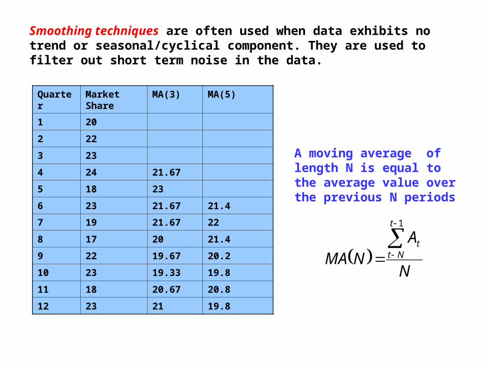
Smoothing techniques are often used when data exhibits no trend or seasonal/cyclical component. They are used to filter out short term noise in the data.


MA(3) MA(5)

1 20

2 22

3 23

4 24 21.67

5 18 23

6 23 21.67 21.4

7 19 21.67 22

8 17 20 21.4

9 22 19.67 20.2

10 23 19.33 19.8

11 18 20.67 20.8

12 23 21 19.8

A moving average of length N is equal to the average value over the previous N periods

N

ANMA

t

Ntt

1

0

5

10

15

20

25

30

1 2 3 4 5 6 7 8 9 10 11 12

Actual

MA(3)

MA(5)

The longer the moving average, the smoother the forecasts are…


MA(3) MA(5)

1 20

2 22

3 23

4 24 21.67

5 18 23

6 23 21.67 21.4

7 19 21.67 22

8 17 20 21.4

9 22 19.67 20.2

10 23 19.33 19.8

11 18 20.67 20.8

12 23 21 19.8

Calculating forecasts is straightforward…

MA(3)

33.213

231823

MA(5)

6.205

1722231823

So, how do we choose N??


MA(3) Squared Error

MA(5) Squared Error

1 20

2 22

3 23

4 24 21.67 5.4289

5 18 23 25

6 23 21.67 1.7689 21.4 2.56

7 19 21.67 7.1289 22 9

8 17 20 9 21.4 19.36

9 22 19.67 5.4289 20.2 3.24

10 23 19.33 13.4689 19.8 10.24

11 18 20.67 7.1289 20.8 7.84

12 23 21 4 19.8 10.24

Total = 78.3534 Total = 62.48

95.29

3534.78RMSE 99.2

7

48.62RMSE

Exponential smoothing involves a forecast equation that takes the following form

ttt FwwAF 11

Forecast for time t+1

Actual value at time t

Forecast for time t

Smoothing parameter

Note: when w = 1, your forecast is equal to the previous value. When w = 0, your forecast is a constant.

1,0w


W=.3 W=.5

1 20 21.0 21.0

2 22 20.7 20.5

3 23 21.1 21.3

4 24 21.7 22.2

5 18 22.4 23.1

6 23 21.1 20.6

7 19 21.7 21.8

8 17 20.9 20.4

9 22 19.7 18.7

10 23 20.4 20.4

11 18 21.2 21.7

12 23 20.2 19.9

For exponential smoothing, we need to choose a value for the weighting formula as well as an initial forecast

Usually, the initial forecast is chosen to equal the sample average

8.216.205.235.

0

5

10

15

20

25

30

1 2 3 4 5 6 7 8 9 10 11 12

Actual w=.3 w=.5

As was mentioned earlier, the smaller w will produce a smoother forecast

Calculating forecasts is straightforward…

W=.3

04.212.207.233.

W=.5

45.219.195.235.

So, how do we choose W??


W=.3 W=.5

1 20 21.0 21.0

2 22 20.7 20.5

3 23 21.1 21.3

4 24 21.7 22.2

5 18 22.4 23.1

6 23 21.1 20.6

7 19 21.7 21.8

8 17 20.9 20.4

9 22 19.7 18.7

10 23 20.4 20.4

11 18 21.2 21.7

12 23 20.2 19.9


W = .3 Squared Error

W=.5 Squared Error

1 20 21.0 1 21.0 1

2 22 20.7 1.69 20.5 2.25

3 23 21.1 3.61 21.3 2.89

4 24 21.7 5.29 22.2 3.24

5 18 22.4 19.36 23.1 26.01

6 23 21.1 3.61 20.6 5.76

7 19 21.7 7.29 21.8 7.84

8 17 20.9 15.21 20.4 11.56

9 22 19.7 5.29 18.7 10.89

10 23 20.4 6.76 20.4 6.76

11 18 21.2 10.24 21.7 13.69

12 23 20.2 7.84 19.9 9.61

Total = 87.19 Total = 101.5

70.212

19.87RMSE 91.2

12

5.101RMSE

Economics of the Firm Consumer Demand Analysis. Today’s Plan: Motivation Refresher on Probability...

Documents

Transcript of Economics of the Firm Consumer Demand Analysis. Today’s Plan: Motivation Refresher on Probability...