Economics Lecture 5 - Univerzita Karlovavitali/documentsCourses/Lecture 5 - Price... · 2 Firms,...

Economics Lecture 5

2016-17

Sebastiano Vitali

Course Outline

1 Consumer theory and its applications

1.1 Preferences and utility

1.2 Utility maximization and uncompensated demand

1.3 Expenditure minimization and compensated demand

1.4 Price changes and welfare

1.5 Labour supply, taxes and benefits

1.6 Saving and borrowing

2 Firms, costs and profit maximization

2.1 Firms and costs

2.2 Profit maximization and costs for a price taking firm

3. Industrial organization

3.1 Perfect competition and monopoly

3.2 Oligopoly and games

1.4 Price changes and

welfare

1.4 Price changes and welfare

1. Price indices

2. Substitution bias

3. Compensating variation (CV)

4. Equivalent variation (EV)

5. Compensating variation vs Equivalent variation

6. Compensating variation, equivalent variation and

change in consumer surplus

7. Income effects, CV, EV and consumer surplus

8. Using EV to assess the effect of a tax

9. Using EV to assess the effect of a subsidy

9. Does compensating a consumer for a price increase

imply that the price increase has no effect on demand?

10. Benefits in kind

Base weighted price

indices

1. Price indices measure inflation

• Public sector use

• Inflation targeting

• Adjusting levels of taxes, benefits, public pensions

• Indexed government bonds

• Measurement of real wages

• Private sector use

• Pensions

• Measurement of real wages

• Price & wage setting

The design of price indices matters and is

controversial

• Prices of different things change at different rates.

• Price indices are weighted averages

• What should be included in the index?

• Weights

• Formula

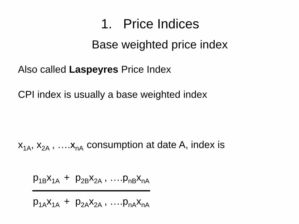
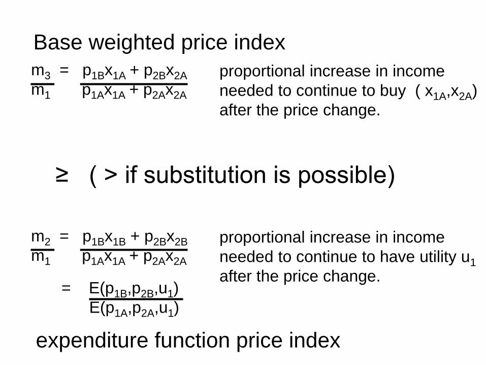
p1Bx1A + p2Bx2A , ….pnBxnA

p1Ax1A + p2Ax2A , ….pnAxnA

Also called Laspeyres Price Index

CPI index is usually a base weighted index

x1A, x2A , ….xnA consumption at date A, index is

1. Price Indices

Base weighted price index

= w1 p1B + w2 p2B + …………+ wn pnB

p1A p2A pnA

where w1 = p1A x1A etc.


The base weighted price index is a weighted average of

proportionate price increases where weight for good i is

the proportion of expenditure spent on good i at date A.

p1Bx1A + p2Bx2A , ….pnBxnA


Base weighted

price index

Consumer Price Index (CPI)

CPI is essentially base weighted indices but the weights

change over time as expenditure patterns change.

European Union Consumer Price Indices:

CPI

Czech republic Consumer Price Indices:

CPI

European Union CPI of different goods.

Gen 2017, Source www.ecb.europa.eu

European Union weights to different goods.

Gen 2017, Source www.ecb.europa.eu

Price indices and

substitution bias

p1Bx1A + p2Bx2A

p1Ax1A + p2Ax2A

E(p1B,p2B,u)

E(p1A,p2A,u)

The base weighted price index

measures the proportional increase

in the cost of (x1A,x2A)

The expenditure function price index

measures the proportional increase

in the cost of getting utility u

Fact: base weighted index ≥ expenditure function price index.

The next slides explain why.

2. Substitution bias

x2

0 x1

gradient

– p1A/p2A

( x1A,x2A)

m3/p2B

m2/p2B

m1/p2A

(x1A, x2A) maximizes

utility subject to the

budget constraint

p1Ax1 + p2Ax2 = m1

(x1A, x2A) is the

cheapest way of getting

utility u1 at prices

(p1A,p2A) so the

expenditure function

E(p1A,p2A,u1)

= p1Ax1A + p2Ax2A = m1

u1

x2

0 x1

gradient– p1B/p2B

( x1A,x2A)

m3 = p1Bx1A + p2Bx2A

is the cost of ( x1A,x2A)

at prices (p1B,p2B)

m1 = p1Ax1A + p2Ax2A

is the cost of ( x1A,x2A)

at prices (p1A,p2A).

u1


m1 p1Ax1A + p2Ax2A

m3/p2B

m2/p2B

m1/p2A

proportional increase in income

needed to continue to buy (x1A,x2A)

after the price change

= base weighted price index.

x2

0 x1

gradient– p1B/p2B

( x1A,x2A)

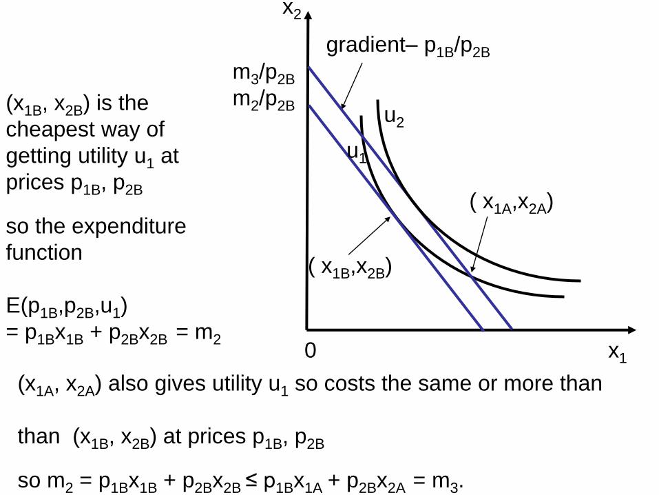
( x1B,x2B)

(x1B, x2B) is the

cheapest way of

getting utility u1 at

prices p1B, p2B

so the expenditure

function

E(p1B,p2B,u1)

= p1Bx1B + p2Bx2B = m2

(x1A, x2A) also gives utility u1 so costs the same or more than

than (x1B, x2B) at prices p1B, p2B

so m2 = p1Bx1B + p2Bx2B ≤ p1Bx1A + p2Bx2A = m3.

m3/p2B

m2/p2B

m1/p2A

u1

u2

x2

0 x1

gradient– p1B/p2B

( x1A,x2A)

( x1B,x2B)

m3/p2B

m2/p2B

m1/p2A

u1

u2

Here m2 < m3 so a consumer with income m3 has higher

utility than a consumer with income m2.

x2

0 x1

gradient– p1B/p2B

gradient

– p1A/p2A

( x1A,x2A)

( x1B,x2B)

m3/p2B

m2/p2B

m1/p2A

If prices change from (p1A,p2A) to (p1B,p2B) and income

changes from m1 to m2 utility does not change.

If prices change from (p1A,p2A) to (p1B,p2B) and income

changes from m1 to m3 utility increases.

u1

u2


m1 p1Ax1A + p2Ax2A


needed to continue to buy ( x1A,x2A)

after the price change.

m2 = p1Bx1B + p2Bx2B

m1 p1Ax1A + p2Ax2A

= E(p1B,p2B,u1)

E(p1A,p2A,u1)


needed to continue to have utility u1

after the price change.

Base weighted price index

≥ ( > if substitution is possible)

expenditure function price index

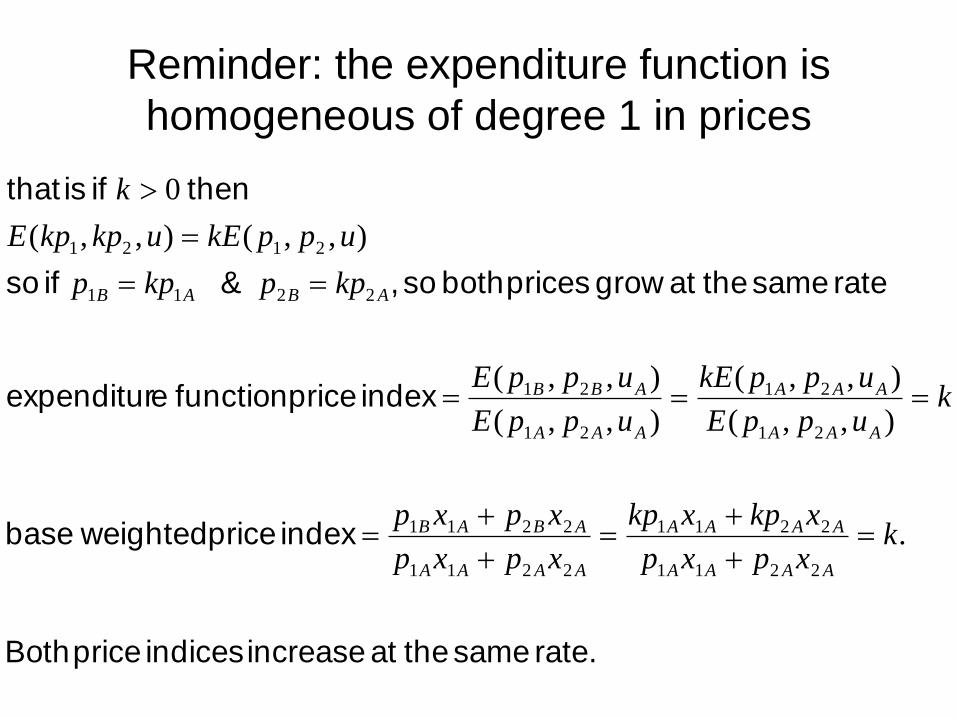
Reminder: the expenditure function is

homogeneous of degree 1 in prices

rate. same the at increase indices price Both

index price weightedbase

index price function eexpenditur

rate same the atgrow prices both so , & if so

then if is that

.

),,(

),,(

),,(

),,(

),,(),,(

0

2211

2211

2211

2211

21

21

21

21

2211

2121

kxpxp

xkpxkp

xpxp

xpxp

kuppE

uppkE

uppE

uppE

kppkpp

uppkEukpkpE

k

AAAA

AAAA

AAAA

ABAB

AAA

AAA

AAA

ABB

ABAB

Substitution bias

• If prices do not all grow at the same rate

• & there is a substitution effect

• base weighted price index

> expenditure function price index.

Substitution bias

If income grows at the same rate as a base weighted price

index utility either increases or stays the same.

If there is any possibility of substitution utility increases.

Thus base weighted price indices overstate the rate of

inflation.

Over the long term the introduction of new

goods is a big issue for price indices.

Who today would buy a film stored on

this?

Who in 1990 downloaded a film from

the internet?

www.freephoto1.com

© Getty Images

Problems with the expenditure function price

index

• Calculating the expenditure function price index requires

knowledge of the expenditure function.

• The expenditure function is derived from the utility

function.

• The utility function is unobservable.

• There is a neat way round this for situations where only

one price changes.

• This is the compensating and equivalent variation

developed by Hicks which turn out to be closely related

to consumer surplus.

Compensating variation

CV

The compensating variation for a price increase from p1A to

p1B is the amount of extra money the consumer needs to

get back to the same level of utility as before the price

change.

3. Compensating variation (CV)

Definition

Compensating variation and the expenditure

function

At prices (p1A,p2) the consumer buys (x1A,x2A) giving utility

u(x1A,x2A) = uA.

After the price change & compensation the consumer gets the

same level of utility by buying (x1B,x2B) so u(x1B,x2B) = uA.

The consumer minimises the cost of getting utility so

• the amount spent at prices (p1A,p2) is E(p1A,p2,uA),

• the amount spent at prices (p1B,p2) after compensation is

E(p1B,p2,uA).

• Compensating variation = E(p1B,p2,uA) - E(p1A,p2,uA)

0 x1


A

x2

0 x1

x2


A

E(p1A,p2,uA)

p2

E(p1B,p2,uA)

p2

CV

p2

0 x1

x2


A

E(p1A,p2,uA)

p2

E(p1B,p2,uA)

p2

CV

p2

How much the consumer

is available to pay more

to maintain same utility

as before price increase

Equivalent variation

EV

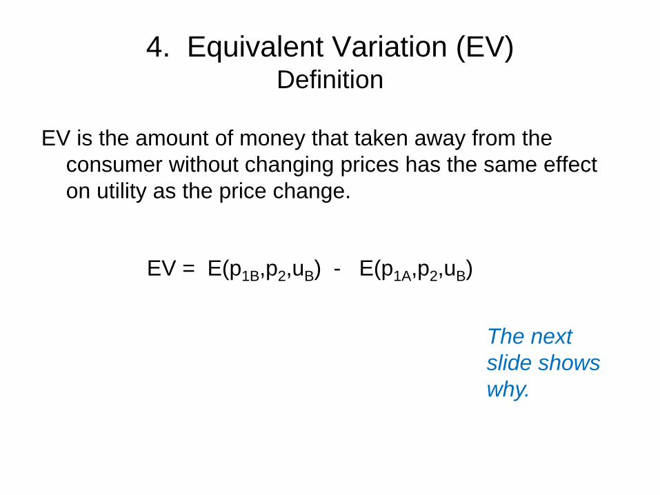
4. Equivalent Variation (EV)Definition

EV is the amount of money that taken away from the

consumer without changing prices has the same effect

on utility as the price change.

EV = E(p1B,p2,uB) - E(p1A,p2,uB)

The next

slide shows

why.

0 x1

x2


A

0 x1

x2


A

x2

E(p1A,p2,uB)

p2

E(p1B,p2,uB)

p2

EV

p2

0 x1

x2


A

x2

E(p1A,p2,uB)

p2

E(p1B,p2,uB)

p2

EV

p2

How much the consumer

is available to income

less in order to avoid

price increase

0 x1

x2

5. Compensated variation vs


AE(p1A,p2,uB)

p2

EV

p2

E(p1B,p2,uA)

p2

CV

p2E(p1B,p2,uB)

p2

E(p1A,p2,uA)

p2=

CV = E(p1B,p2,uA) - E(p1A,p2,uA)


Compensated variation vs Equivalent variation

Compensated variation = we measure it on the

compensated demand on initial utility indifference curve.

When price changes and we want to keep same utility,

how much are we willing to pay?

Equivalent variation = we measure it on the compensated

demand on new utility indifference curve. When price

changes how much are we willing to pay to go back to

previous utility?



Compensated variation vs Equivalent variation

Compensated variation =

price changes

how much does it cost to keep same utility?


Equivalent variation =

price changes

utility reduces

how much would we save to have the same new utility if

the prices would not change?


Is it possible to measure

CV and EV with

compensated and

uncompensated demand

function?

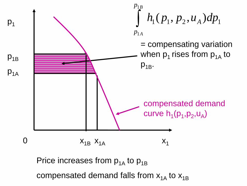
CV and Shephard’s Lemma

• The problem remains, CV depends on the expenditure

function so depends on utility so it is unobservable.

• Remember Shephard’s lemma

• To work with this you need to remember the relationship

between differentiation and integration.

𝜕𝐸(𝑝1, 𝑝2, 𝑢)

𝜕𝑝1= ℎ1(𝑝1, 𝑝2, 𝑢)

0 a b x

y

f’(x)

The relationship between differentiation and

integration

b

a

dxxfaff(b)

xfdx

dy

xfy

)(')(then

)('

)( If

0 x1B x1A x1

p1

p1B

p1A

= compensating variation

when p1 rises from p1A to

p1B.

compensated demand

curve h1(p1,p2,uA)

Price increases from p1A to p1B

compensated demand falls from x1A to x1B

1211 ),,(1

1

dpupph A

p

p

B

A

Shephard’s lemma

implies that

CV and Shephard’s Lemma

𝑝1𝐴𝑝1𝐵 ℎ1(𝑝1, 𝑝2 , 𝑢)𝑑𝑝1= E(𝑝1𝐵 , 𝑝2,u) - E(𝑝1𝐴, 𝑝2,u)

𝜕𝐸(𝑝1, 𝑝2, 𝑢)

𝜕𝑝1= ℎ1(𝑝1, 𝑝2, 𝑢)

0 x1


x1(p1,p2 ,m)

Demand curve diagram

uA is the level of utility that the consumer gets with

prices (p1A,p2) and income m.

p1A

compensated demand

h1(p1,p2 ,uA)

p1A

0 x1


x1(p1,p2 ,m)

Compensated demand is less elastic than

uncompensated demand.

Income and substitution effects work in the

same direction. This is a normal good


compensated demand

h1(p1,p2 ,uA)

p1B

p1A

0 x1


x1(p1,p2 ,m)


compensated demand

h1(p1,p2 ,uA)

compensated demand

h1(p1,p2 ,uA)p1B

p1A

0 x1


x1(p1,p2 ,m)

compensated demand

h1(p1,p2 ,uB)


uB is the level of

utility that the

consumer gets with

prices (p1B,p2) and

income m.

p1B

p1A

0 x1

Compensating

Variation ACDF


compensated demand

h1(p1,p2 ,uA)A B C

F E D

compensated demand

h1(p1,p2 ,uB)

compensated demand

h1(p1,p2 ,uA)p1B

p1A

0 x1

EV Equivalent Variation ABEF


x1(p1,p2 ,m)


A B C

F E D

compensated demand

h1(p1,p2 ,uB)

compensated demand

h1(p1,p2 ,uA)p1B

p1A

0 x1

Normal good

EV < CV

ABEF ACDF


x1(p1,p2 ,m)


A B C

F E D

compensated demand

h1(p1,p2 ,uB)

Normal goods, CV & EV

Uncompensated demand is more elastic than compensated

demand because income and substitution effects work in

the same direction.

For a price rise

EV < CV

because EV is measured at a lower level of utility.

As the good is normal, it is less consumed at lower utility.

Compensating variation,

equivalent variation and

change in consumer

surplus

p1B

p1A

0 x1

Compensating

Variation ACDF


6. Compensating variation, equivalent variation

and change in consumer surplus

F E D

A B C

compensated demand

h1(p1,p2 ,uA)

compensated demand

h1(p1,p2 ,uA)p1B

p1A

0 x1

EV Equivalent Variation ABEF


x1(p1,p2 ,m)


A B C

F E D

compensated demand

h1(p1,p2 ,uB)

p1B

p1A

0 x1


x1(p1,p2 ,m)

A B C

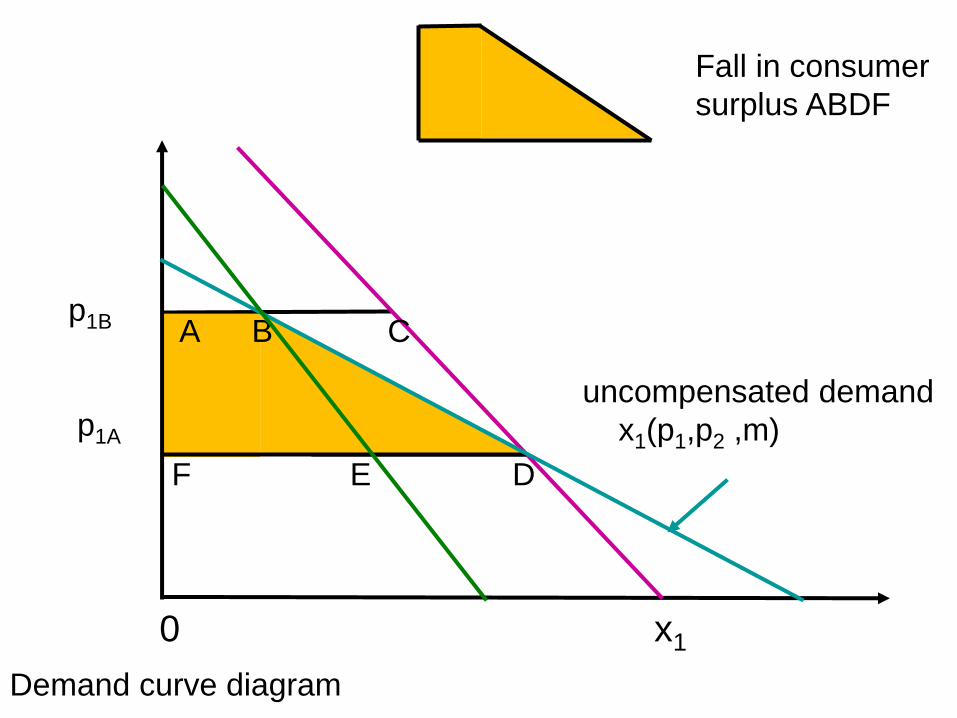
F E D

Fall in consumer

surplus ABDF


compensated demand

h1(p1,p2 ,uA)p1B

p1A

0 x1

Normal good

EV < change CS < CV

ABEF ABDF ACDF


x1(p1,p2 ,m)


A B C

F E D

compensated demand

h1(p1,p2 ,uB)

Normal goods, CV, consumer surplus & EV

Change in Consumer Surplus is the area bounded by the

uncompensated demand curve.

Compensating variation is the area bounded by the

compensated demand curve with utility uA.

Equivalent variation is the area bounded by the

compensated demand curve with utility uB.

For a price rise

EV < change in consumer surplus < CV

Income effects, CV, EV and

consumer surplus

7. Income effects, CV, EV and consumer

surplus

When there are no income effects uncompensated and

compensated demand are the same so

the loss in consumer surplus due to an increase in p1 is

the same as the CV & EV.

The difference between CV, EV and the change in

consumer surplus is due to income effect.

The Slutsky equation in elasticities

shows the size of the income effect

m

xp

m

x

x

m

p

h

h

p

p

x

x

p 111

11

1

1

1

1

1

1

1

m

xp

m

x

x

m

p

h

h

p

p

x

x

p 111

11

1

1

1

1

1

1

1

Own price elasticity

of uncompensated

demand

Own price elasticity

of compensated

demand

Income elasticity of

uncompensated

demand

budget

sharesubstitution

effectincome effect

Income effects are small when either or both of the income

elasticity of uncompensated demand and the budget share are

small.

If income effects are small the change in consumer surplus is a

good approximation to the compensating variation.

Which measure to use?

If income effects are small, for example because the budget

share is small, CV, EV and change in CS are close. Use

change in CS because it is easy to measure.

If income effects are large, it depends on the question you

want to answer.

CV if it is how much is needed to compensate.

EV if it is what is the monetary equivalent of the price

change.

Examples

A government wants to reduce CO2 generation to combat

global warming.

Fuel is a large share of expenditure so the income effect is

significant.

The gov does this through taxation.

To make this politically acceptable the gov needs to

compensate people for the increase in tax, the

compensating variation is relevant. For instance

increasing public investment in green areas.

Otherwise if the gov wants to make some tax reduction to

balance, he has to measure the monetary effect with the

equivalent variation.

When does an increase in price from p1A to p1B

have a big adverse impact on the consumer?

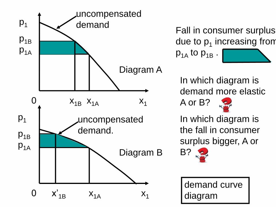
0 x’1B x1A x1

Diagram A

Diagram B

0 x1B x1A x1

p1

p1B

p1A

uncompensated

demand

p1

p1B

p1A

uncompensated

demand.

Fall in consumer surplus

due to p1 increasing from

p1A to p1B .

demand curve

diagram

In which diagram is

demand more elastic

A or B?

In which diagram is

the fall in consumer

surplus bigger, A or

B?

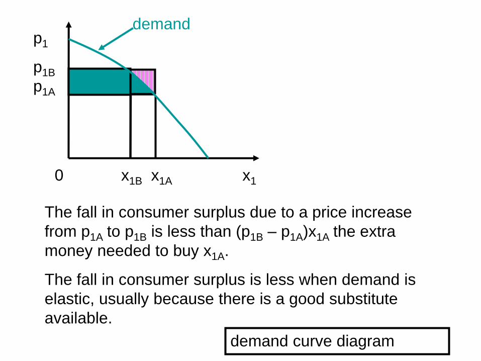
0 x1B x1A x1

p1

p1B

p1A

demand

The fall in consumer surplus due to a price increase

from p1A to p1B is less than (p1B – p1A)x1A the extra

money needed to buy x1A.

The fall in consumer surplus is less when demand is

elastic, usually because there is a good substitute

available.

demand curve diagram

1111

1111111

2

1

))((2

1)(

xpxp

xxppxpp

A

BAABAAB

fall in consumer surplus = -

0 x1B x1A x1

p1

p1B

p1A

demandFormula for fall into

consumer surplus.

Let Δp1 = p1B – p1A > 0

Let Δx1 = x1B – x1A < 0

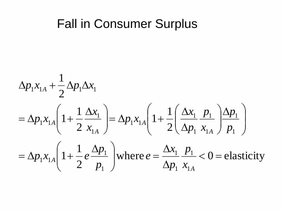
elasticity 0 where2

11

2

11

2

11

2

1

1

1

1

1

1

111

1

1

1

1

1

111

1

111

1111

A

A

A

A

A

A

A

x

p

p

xe

p

pexp

p

p

x

p

p

xxp

x

xxp

xpxp

Fall in Consumer Surplus

increase price ateproportion

0demand of elasticity priceown

buying ofcost in the increase theis

where

2

11 surplusconsumer in Fall

1

1

1

1

1

1

111

1

111

A

A

A

AA

A

A

p

p

x

p

p

xe

xxp

p

pexp

The fall in consumer surplus is less when

demand is more elastic.

The higher the elasticity, since it is negative, the less the

fall in consumer surplus

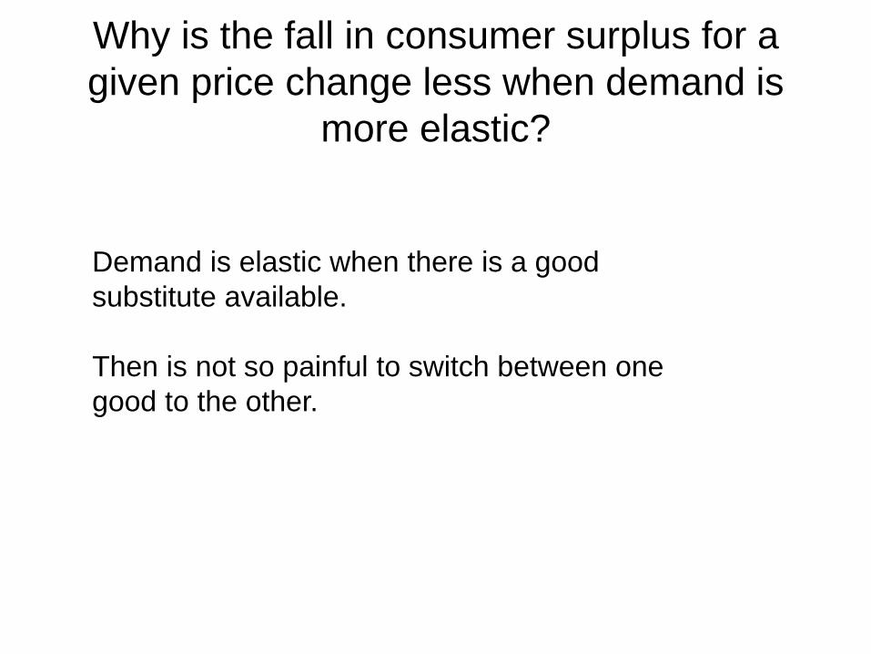
Why is the fall in consumer surplus for a

given price change less when demand is

more elastic?

Demand is elastic when there is a good

substitute available.

Then is not so painful to switch between one

good to the other.

When does an increase in price from p1A to p1B

have a big adverse impact on the consumer?

Inelastic demand

Steep demand curve

No close substitute available

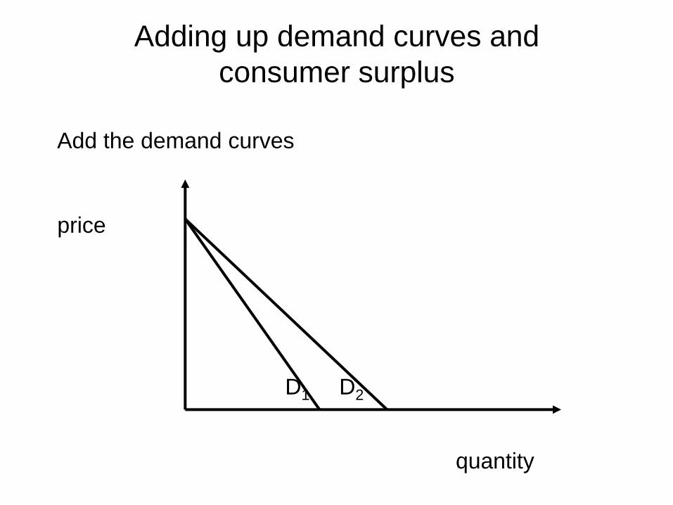
Add the demand curves

price

quantity

D1 D2

Adding up demand curves and

consumer surplus

price

quantity


consumer surplus

D1 D2 D1 + D2

Add the demand curves horizontally

price

quantity


consumer surplus

D1 D2 D1 + D2

p1B

p1A

Shaded area

= loss of consumer surplus from

group 1

+ loss of consumer from group 2

Add the demand curves

Each person in group 1 earns €8,000 per year.

Each person in group 2 earns €100,000 per year,

There are 100 people in each group.

Situation 1, everyone in group 1 losses CS €250, everyone in

group 2 looses CS €50. Total loss CS

=



=






= 100 x €250 + 100 x €50= €30000.



=






= 100 x €250 + 100 x €50= €30000.



= 100 x €50 + 100 x €250= €30000.

Adding up consumer surplus geometrically implies a value

judgement that giving €1 to one consumer has the same

social benefit as giving €1 to any other consumer.

If you disagree with this judgement you would want to

evaluate the losses to each group, and then consider how

to use them as input into a decision.

This can be modelled mathematically.

Very important

Using equivalent variation to

assess the effect of a tax

Suppose that a tax causes the price of good 1 to rise from

p1A to p1A + t, where t is tax. (This is called an excise

tax.)

(We will see later that this is a special case, it happens

when supply is perfectly elastic.)

Demand for good 1 falls from x1A to x1B. Demand for good 2

rises from x2A to x2B.

How much revenue does the tax raise?

8. Using EV to assess the effect of a tax

Tax revenue t x1B

Good 2 is expenditure on other goods, assume p2 = 1.

From the budget constraint without tax

p1A x1A + x2A = m

budget constraint with tax

(p1A + t) x1B + x2B = m

Subtract these equations to get

(p1A x1A + x2A ) – (p1Ax1B + x2B) - t x1B = 0.


(p1A x1A + x2A ) – (p1Ax1B + x2B) - t x1B = 0.

So tax revenue = t x1B = (p1Ax1A + x2A) – (p1A x1B + x2B)

Cost of original

combination (x1A,x2A)

at prices p1A, p2

Cost of new

combination (x1B,x2B)

at prices p1A, p2

budget line with tax,

new prices

slope – (p1A + t)IC diagram, p2 = 1

0 x1

budget lines without tax,

original prices

slope – p1A

(x1A,x2A)(x1B,x2B)

Tax revenue

EV

Excess burden =

EV – tax revenueA

B

x2

IC diagram, p2 = 1

0 x1

(x1A,x2A)(x1B,x2B)

A

B

x2


new prices

slope – (p1A + t)


original prices

slope – p1A

Tax revenue AB

EV

Excess burden =

EV – tax revenue

IC diagram, p2 = 1

0 x1

(x1A,x2A)(x1B,x2B)

Tax revenue AB

EV

Excess burden =

EV – tax revenueA

B

C

x2


new prices

slope – (p1A + t)


original prices

slope – p1A

IC diagram, p2 = 1

0 x1

(x1A,x2A)(x1B,x2B)

Tax revenue AB

EV AC

Excess burden =

EV – tax revenueA

B

C

x2


new prices

slope – (p1A + t)


original prices

slope – p1A

IC diagram, p2 = 1

0 x1

(x1A,x2A)(x1B,x2B)

Tax revenue AB

EV AC

Excess burden =

EV – tax revenue A

B

C

x2


new prices

slope – (p1A + t)


original prices

slope – p1A

budget line with tax

slope – (p1A + t)

IC diagram, p2 = 1

0 x1

budget lines without tax

slope – p1A

(x1A,x2A)(x1B,x2B)

Tax revenue AB

EV AC

Excess burden =

EV – tax revenue BCA

B

C

x2

Definition: The excess burden of an excise tax is

EV – tax revenue = monetary loss to consumer – tax revenue

The total society benefit decreases by EV and increases by

the tax revenue, but in total it decreases by the excess

burden

With an excise tax there is an excess burden.

Suppose that instead of a excise tax t, the government

imposed a “lump sum” tax that took away R from the

consumer so the budget constraint is

p1Ax1 + p2 x2 = m – R.

With R = t x1B

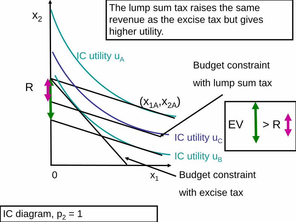
IC diagram, p2 = 1

IC utility uA

IC utility uB

(x1A,x2A)

R

IC utility uC

Budget constraint

with lump sum tax

Budget constraint

with excise tax

The lump sum tax raises the same

revenue as the excise tax but gives

higher utility.

0 x1

x2

EV > R

This is a general argument.

Suppose the government wants to raise revenue R.

A lump sum tax that reduces income by R that does not

depend on anything the consumer does reduces utility

by less than a tax raises R where the revenue could be

changed by changing consumption, work or saving.

(e.g. excise tax, VAT, income tax…)

The only feasible lump sum tax is a “poll tax” where

everyone pays the same amount.

Is a poll tax ethically desirable?

Is a poll tax politically feasible?

Using equivalent variation to

assess the effect of a

subsidy.

Suppose that a subsidy causes the price of good 1 to fall

from p1A to p1A - s , where s is the subsidy per unit.

Demand for good 1 changes from x1A to x1C. Demand for

good 2 changes from x2A to x2C.

How much does the subsidy cost?

9. Using EV to assess the effect of a subsidy.

budget line

with subsidy

slope – (p1A - s)

IC diagram, p2 = 1

budget line without

subsidy slope – p1A

(x1A,x2A)

0 x1

x2

(x1C,x2C)

m

Subsidy costs s x1C

Good 2 is expenditure on other goods so p2 = 1.

From the budget constraint without subsidy

p1A x1A + x2A = m

budget constraint with subsidy

(p1A - s) x1C + x2C = m


(p1A x1A + x2A ) – (p1Ax1C + x2C) + sx1C = 0.


(p1A x1A + x2A ) – (p1Ax1C + x2C) + sx1C = 0.

Rearrange cost of subsidy

= s x1C = (p1A x1C + x2C) - (p1A x1A + x2A)

Cost of original bundle

(x1A,x2A) at prices

p1A, p2 = 1.

Cost of new bundle

(x1C,x2C) at prices

p1A, p2 = 1.

IC diagram, p2 = 1

budget lines gradient – p1A

(x1A,x2A)

(x1C,x2C)

0 x1

x2

A

B

C

Cost of subsidy? AC

budget line with subsidy

gradient – (p1A – s)

The equivalent variation (EV) of a

subsidy is the amount of extra income

the consumer needs to get to have

the same effect on utility as the

subsidy.

IC diagram, p2 = 1

(x1A,x2A)

(x1C,x2C)

0 x1

x2

A

B

C

Cost of subsidy?

Equivalent variation? BC




x2

A

B

C

IC diagram, p2 = 1

(x1A,x2A)

(x1C,x2C)

0 x1

x2

A

B

C


Cost of subsidy? AC

Equivalent variation? BC



IC diagram, p2 = 1

budget line without

subsidy gradient – p1A

(x1A,x2A)

(x1C,x2C)

0 x1

x2

A

B

C

Cost of subsidy? AC

> equivalent variation BC



General argument

• A lump sum subsidy increases income by a fixed amount

that does not depend on anything the consumer does

• Increasing the consumer’s utility by giving the EV as a

lump sum

costs less than increasing the consumer’s utility by

the same amount using a subsidy.

• So either the state can save some money and get the

same EV, or can use the same amount of money and

get a higher EV (higher utility) as in next slide

IC diagram, p2 = 1

budget line without

subsidy gradient – p1A

(x1A,x2A)

(x1C,x2C)

0 x1

x2

A

B

C

Cost of subsidy? AC

> equivalent variation BC



Does compensating a

consumer for a price

increase imply that the

price increase has no

effect on demand?

Suppose a price (e.g. heating fuel) rises from p1A to p1B .

Demand for the good falls.

Suppose the consumer is compensated by being given the

compensating variation (CV). Does the consumer go

back to consuming the same amount of heating fuel?

10. Does compensating a consumer for a

price increase imply that the price increase

has no effect on demand?

budget

line after

price

change

gradient

– p1B

IC diagram, p2 = 1

budget line before price

change gradient – p1A

IC utility uA

IC utility uB

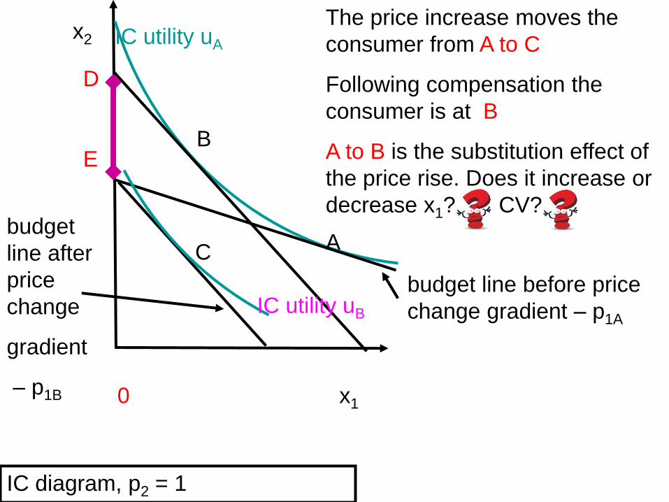
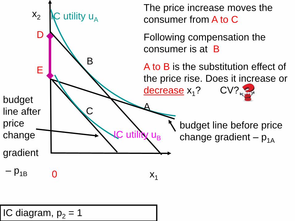
The price increase moves the

consumer from

Following compensation the

consumer is at

is the substitution effect of

the price rise. Does it increase or

decrease x1? CV?

A

B

C

0 x1

x2

TP

budget

line after

price

change

gradient

– p1B

IC diagram, p2 = 1



IC utility uA

IC utility uB


consumer from A to C.


consumer is at



decrease x1? CV?

A

B

C

0 x1

x2

budget

line after

price

change

gradient

– p1B

IC diagram, p2 = 1



IC utility uA

IC utility uB


consumer from A to C


consumer is at B



decrease x1? CV?

A

0 x1

x2

D

EB

C

budget

line after

price

change

gradient

– p1B

IC diagram, p2 = 1



IC utility uA

IC utility uB




consumer is at B

A to B is the substitution effect of


decrease x1? CV?

A

0 x1

x2

D

EB

C

budget

line after

price

change

gradient

– p1B

IC diagram, p2 = 1



IC utility uA

IC utility uB




consumer is at B

A to B is the substitution effect of


decrease x1? CV? DE

A

0 x1

x2

D

EB

C

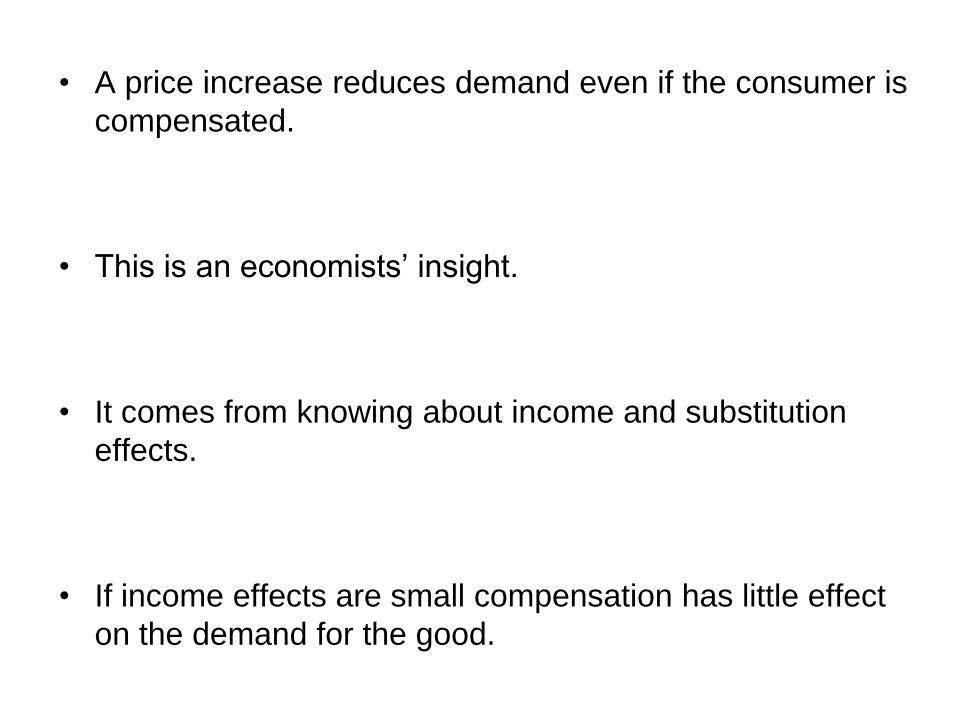
• A price increase reduces demand even if the consumer is

compensated.

• This is an economists’ insight.

• It comes from knowing about income and substitution

effects.

• If income effects are small compensation has little effect

on the demand for the good.

Have you received a present and thought

you would rather have the money it cost?

1. often

2. rarely

3. never

Benefits in kind

budget line

with benefit in kind

0 x1D x1

x2

m

budget line without

benefit in kind

The consumer gets a

benefit in kind, getting

x1D units of good 1

costing p1x1D for free.

11. Benefits in Kind

0 x1D x1

x2

m

budget line without

benefit in kind

budget line with

extra incomeIn this figure would the

consumer be better off

just getting the money

as extra income?

0 x1D x1

x2

m

budget line without

benefit in kind

budget line with

extra incomeIn this figure would the



as extra income?

No

IC diagram, p2 = 1

0 x1D x1

x2

m

budget line without

benefit in kind

In this figure would the



as extra income?

budget line with

extra income

IC diagram, p2 = 1

0 x1D x1

x2

m

budget line without

benefit in kind

In this figure would the



as extra income?

Yes

budget line with

extra income

Why Benefits in Kind?

The last slides suggest that it is sometimes better and never worse

for a consumer to get a sum of money rather than a benefit in

kind costing the same amount.

So why are benefits in kind common?

Students Across The UK Return To School For Start Of The Autumn Term

Clinical Trials Begin For New Vaccine Against Avian Influenza © Getty Images

Why do

governments

provide health and

education free at

the point of service?

Price changes and welfare.

What have we achieved?

• Understanding of uses and limitations of price indices.

• Monetary measures of impact of price changes on

consumer’s welfare, & the implicit value judgement.

• Application of these measures to taxes & subsidies

• Change in consumer surplus, compensating &

equivalent variation.

• Insights on effect of compensation on consumer

demand.

Economics Lecture 5 - Univerzita Karlovavitali/documentsCourses/Lecture 5 - Price... · 2 Firms,...

Documents

Transcript of Economics Lecture 5 - Univerzita Karlovavitali/documentsCourses/Lecture 5 - Price... · 2 Firms,...