Economics Department Working Paper Series

No. 10-2010

Aid Absorption and Spending in Africa:A Panel Cointegration Approach

Pedro M. G. Martins

Institute of Development Studies (IDS)University of Sussex

pedromgmartins@gmail.com

Abstract: This paper focuses on the macroeconomic management of large inflows of

foreign aid. It investigates the extent to which African countries have coordinatedfiscal and macroeconomic responses to aid surges. In practice, we construct a paneldataset to investigate the level of aid ‘absorption’ and ‘spending’. This paper departsfrom the recent empirical literature by utilising better measures for aid inflows and byemploying cointegration analysis. The empirical short-run results suggest that, onaverage, Africa’s low-income countries have absorbed two-thirds of (grant) aidreceipts. This suggests that most of the foreign exchange provided by the aid inflowshas been used to finance imports. The other third has been used to build upinternational reserves, perhaps to protect economies from future external shocks. Inthe long-run, absorption increases but remains below its maximum (‘full absorption’).Moreover, we also show that aid resources have been fully spent, especially insupport of public investment. There is only weak evidence that a share of aid flowshave been ‘saved’, i.e. substituted domestic borrowing. Overall, these findings

suggest that the macroeconomic management of aid inflows in Africa has beensignificantly better than often portrayed in comparable exercises. The implication isthat African countries will be able to efficiently manage a gradual scaling up in aidresources.

JEL Classification: C23, F35, O23, O55

Key Words: Macroeconomic Management, Foreign Aid, Panel Data, Africa

This paper is based on the author’s DPhil research, which was financially supportedby the Fundação para a Ciência e a Tecnologia.

2

1. Introduction

Foreign aid is often provided with the twin objectives of financing domestic expenditures

and increasing the availability of foreign exchange. In Africa’s low-income countries,

external grants and concessional loans provide crucial resources to support the expansion

of public investment programmes – e.g. building important socio-economic infrastructure

that contributes to fostering economic growth and alleviating poverty. Moreover, these

flows provide foreign exchange resources that allow countries to increase imports of

capital goods, which stimulate economic output and are often associated with productivity

gains.

This paper is mainly concerned with the fiscal and macroeconomic management challenges

arising from large foreign aid inflows. For that purpose, we use the analytical framework

proposed by the IMF (2005) and Hussain et al (2009) to investigate whether African

countries have pursued a coordinated strategy in terms of their fiscal and macroeconomic

responses to large aid inflows. The lack of coordination between the government and the

central bank may undermine the effective use of foreign aid resources, often contributing

to inflationary pressures, the appreciation of the nominal exchange rate, high interest rates

and accumulation of public debt (Buffie et al, 2004).

We construct a new panel dataset for African countries, covering the period 1980-2005. An

important emphasis is placed on the definition, source and construction of the main

variables. Although the vast literature on the macroeconomic impacts of foreign aid

inflows predominantly uses OECD-DAC data on aid, we argue that this is not appropriate.

One reason is that donor-reported statistics often overestimate the ‘true’ amount of aid. For

example, costs relating to technical assistance are included in foreign aid statistics (e.g.

OECD-DAC’s) even though many of these payments never actually leave the donor

country’s banking system. Since these activities have no clear impact on the balance of

payments or the fiscal budget, they should not be included in the analysis. Moreover, off-

budgets are not likely to have significant fiscal effects. Therefore, we favour the use of

official data from recipient countries to assess the questions at hand. In this study we use

balance of payments (BOP) data for the macroeconomic variables (including external

grants) and government data for the fiscal variables. The former is reported in the IMF’s

Balance of Payments Statistics (BOPS) by the respective central banks, whilst the latter is

3

reported in the World Bank’s Africa Database by World Bank country economists. This

actually entails the construction of two different measures of foreign aid.

This paper also strives to use appropriate panel data methodologies. Despite the popularity

of dynamic panel data (DPD) methods in applied research, these seem to be more suitable

for panels with large N (e.g. countries) and small T (observations through time). For panels

that incorporate both a significant number of cross-sections and annual observations – like

this one – non-stationarity becomes a major concern for inference. Therefore, we use

recently developed methods that have strong foundations in the analysis of time series data,

namely, panel unit root tests, cointegration tests, and efficient estimators for assessing

long-run relationships.

The next section provides a brief overview of the literature on the macroeconomic effects

of aid. Moreover, it introduces the analytical framework that provides the background for

this study and presents the few existing empirical results. Section 3 introduces the

empirical methodologies to be utilised in this study. Section 4 explains the construction of

the variables, whereas section 5 presents the empirical findings. Section 6 concludes the

paper.

2. Literature Review

The Macroeconomic Management of Aid

There is a growing literature on the macroeconomic challenges associated with large

foreign aid inflows. White (1992) is an important and often cited early contribution. The

author critically surveys the debates relating to the impact of aid on domestic savings, the

fiscal response, the real exchange rate and ultimately economic growth, thus providing an

excellent synthesis of the theoretical and empirical contributions to the topic. However,

academic interest in these lines of investigation may have suffered from the marked

reduction in aid flows to developing countries during the 1990s. This declining trend was

partly due to: (i) the collapse of the Soviet Union, eliminating the geo-political justification

for providing aid inflows; (ii) rising concerns about the effectiveness of aid in achieving

desired outcomes, namely policy reform, economic growth and poverty reduction (‘aid

fatigue’); and (iii) the economic recession that affected several donors in the early 1990s.

4

Nonetheless, the early 2000s witnessed a renewed interest from the international donor

community. The United Nations Millennium Declaration (and the subsequent Millennium

Development Goals) provided the impetus that was quickly followed by promises to

increase the availability of external finance to developing countries – in particular to

Africa.1 Naturally, this led to the revival of many debates concerning the impact of ‘scaling

up’ aid inflows. The International Monetary Fund took a decisive lead, with publications

such as Isard et al (2006), Heller (2005) and Gupta et al (2006). These works revisit the

main foreign aid debates and provide an overview of current knowledge.

We can subdivide the main issues concerning the macroeconomics of aid into two main

areas: (i) the fiscal sphere, which is influenced by recipient governments; and (ii) the

monetary and exchange rate sphere, which is usually under the responsibility of central

banks. The first incorporates questions about the impact of aid on the size and composition

of public spending, domestic revenues, fiscal deficit, debt sustainability and aid

dependency. This leads to policy decisions such as how much aid the government should

spend and whether it should save some of the aid resources (e.g. to smooth the expenditure

pattern when resources are scarce). The second area focuses on concerns of exchange rate

appreciation, rising price inflation and high interest rates. This often leads to debates about

the optimal level of sterilisation (e.g. Prati et al, 2003) and effective exchange rate regimes

(e.g. Buffie et al, 2004). Nonetheless, these two areas of interest are interdependent and

should be considered in tandem. Fiscal decisions crucially depend on macroeconomic

circumstances (e.g. the interest rate on domestic public debt), while central bank objectives

(e.g. low inflation) are partly influenced by the government’s policy stance. This

interdependence has led to the development of the analytical framework that we will now

discuss.

Analytical Framework

The starting point of this empirical investigation is the analytical framework proposed by

Hussain et al (2009).2 The framework is used to investigate the macroeconomic

management challenges and optimal policy responses to increases (surges) in foreign aid

inflows. This is a crucial policy issue for low-income countries, which are often aid-

1 These were embedded in the 2002 Monterrey Consensus – an outcome of the United Nations International Conferenceon Financing for Development – and the 2005 Gleneagles G8 summit.2 Earlier versions of this paper are Berg et al (2007) and IMF (2005).

5

dependent and may suffer from the volatility and unpredictability of aid flows. Hence, the

framework emphasises the need to coordinate fiscal policy with monetary and exchange

rate policy in order to minimise potential adverse effects and improve its efficiency.

Hussain et al (2009) suggest the use of the following two interrelated concepts: (i)

‘absorption’, which is defined as the widening of the current account deficit (excluding

aid) due to the aid surge; and (ii) ‘spending’, which is defined as the widening of the fiscal

deficit (excluding aid) following an aid surge. Absorption can be seen as a measure of the

degree of ‘real resource transfer,’3 whilst spending assesses “the extent to which the

government uses aid to finance an increase in expenditures or a reduction in taxation”

(Gupta et al, 2006:10). In the special cases of aid-in-kind and ‘tied aid’ (i.e. imports directly

financed by aid), spending and absorption are equivalent.

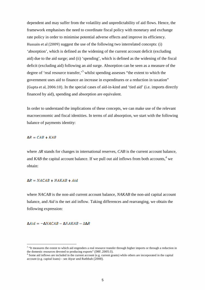
In order to understand the implications of these concepts, we can make use of the relevant

macroeconomic and fiscal identities. In terms of aid absorption, we start with the following

balance of payments identity:

where R stands for changes in international reserves, CAB is the current account balance,

and KAB the capital account balance. If we pull out aid inflows from both accounts,4 we

obtain:

where NACAB is the non-aid current account balance, NAKAB the non-aid capital account

balance, and Aid is the net aid inflow. Taking differences and rearranging, we obtain the

following expression:

3 “It measures the extent to which aid engenders a real resource transfer through higher imports or through a reduction inthe domestic resources devoted to producing exports” (IMF, 2005:3).4 Some aid inflows are included in the current account (e.g. current grants) while others are incorporated in the capitalaccount (e.g. capital loans) – see Aiyar and Ruthbah (2008).

6

This identity provides some insights into the possible uses of additional aid inflows: (i) to

widen the non-aid current account deficit (usually through higher imports); (ii) to widen

the non-aid capital account deficit (potentially through capital outflows); and (iii) to

increase the accumulation of international reserves. We can now express aid absorption as

the deterioration of the non-aid current account balance that is attributed to aid (Aiyar and

Ruthbah, 2008):

Assuming that ∆Aid>0, ‘full absorption’ is achieved when the non-aid current account

deficit increases by the same amount of the extra aid inflow (the measure equals 1). A

value close to 0 indicates a low level of absorption, and suggests that the additional foreign

exchange provided by the aid inflow is used to increase international reserves and/or widen

the non-aid capital account deficit.

In terms of aid spending, we start from the usual budget constraint facing the government:

where IG stands for public investment, CG public recurrent expenditures, T domestic

revenue, B domestic borrowing and L external (non-concessional) loans. Re-arranging the

budget constraint and differencing we obtain:

where NAGOB is the non-aid government overall balance, i.e. domestic revenues (T) minus

total expenditures (IG + CG). Hence, the potential uses of the additional aid inflows are: (i)

to widen the non-aid current account deficit (through higher public spending and/or lower

domestic revenues); and (ii) reduce the need for deficit financing (either domestic or

external). We can now express aid spending as:

7

Similarly, ‘full spending’ is achieved when the additional aid inflows are utilised to expand

the non-aid fiscal deficit (the measure equals 1), whereas a value close to 0 suggests that

aid has not been significantly spent.

Table 1: Possible Combinations in Response to a Scaling Up of AidAbsorbed Not Absorbed

Spent Government spends the aid Central Bank sells the foreign exchange Current account deficit widens

Fiscal deficit widens (expenditures areincreased)

Central Bank does not sell foreignexchange

International reserves are built up Inflation increases

NotSpent

Government expenditures are notincreased

Central Bank sells the foreign exchange Monetary growth is slowed; nominal

exchange rates appreciate; inflation islowered;

Government expenditures are not increased Taxes are not lowered International reserves are built up

Source: Gupta et al (2006:12)

When we take these two concepts together, there are four potential scenarios to be

considered:

(i) Absorb and spend aid. The government spends the extra aid inflow – either through

higher public spending, lower domestic revenue (e.g. cutting taxes), or a mixture of both –

while the central bank sells the foreign exchange in the currency market. The fiscal

expansion stimulates aggregate demand, which in turn contributes to a higher (public and

private) demand for imports. This effect does not create balance of payments problems

since the aid inflow finances the increase in net imports – as more foreign currency

becomes available to importers. Hence, the foreign exchange is absorbed by the economy

through the widening of the non-aid current account deficit (Gupta et al, 2006). This policy

combination leads to aid-financed widening deficits, while the central bank’s balance sheet

remains unaltered (see table below). However, some real exchange rate appreciation may

take place to enable this reallocation of resources. The choice of exchange rate regime will

affect the mechanism through which the (potential) real exchange rate appreciation may

occur – nominal appreciation in a ‘pure float’ versus higher domestic inflation in a ‘fixed

peg’ (Hussain et al, 2009). This absorb-and-spend combination is often considered to be the

ideal policy response to a surge in aid inflows.

8

(ii) Absorb but not spend aid. The government decides not to spend the aid inflow,5 while

the central bank sells the foreign exchange. Foreign aid is thus used to reduce the

government’s seigniorage requirement since it substitutes domestic borrowing in financing

the government deficit (Buffie et al, 2004). Moreover, the central bank sterilises the

monetary impact of domestically financed fiscal deficits (Gupta et al, 2006). This policy

scenario usually leads to slower monetary growth and alleviates inflationary pressures.

Hussain et al (2009) suggest that this could be an appropriate policy response in countries

that have not achieved stabilisation – hence facing high domestic deficits and high inflation

– or have a large stock of domestic public debt. A reduction in the level of outstanding

public debt could ‘crowd in’ the private sector (both investment and consumption) through

its effect on interest rates (Hussain et al, 2009).6 This increase in aggregate demand would

then feed into higher net imports, which would then be financed by the additional foreign

exchange available in the currency market.

(iii) Spend and not absorb aid. The government spends the additional aid inflow (non-aid

fiscal deficit widens), while the central bank allows its foreign exchange reserves to

increase. In this case, the extra foreign exchange is not made available to importers but

instead is used to build up international reserves. This policy response is similar to a fiscal

stimulus in the absence of foreign aid (Hussain et al, 2009). The increase in government

spending must be financed by either: (i) monetising the fiscal expansion (i.e. printing

domestic currency), which increases money supply and therefore inflation; or (ii)

sterilising the monetary expansion (by issuing securities, usually treasury bills), which

could lead to higher interest rates and potentially crowd out the private sector (Hussain et

al, 2009). There is no real resource transfer due to the absence of an increase in net imports.

The IMF (2005) argues that this is a “common but problematic response, often reflecting

inadequate coordination of monetary and fiscal policies.” The net effect on the real

exchange rate is uncertain: higher (unmet) demand for net imports contributes to

depreciation (via the nominal exchange rate), whilst higher inflation works in the opposite

way.

5 It is assumed that neither public spending is increased nor revenues lowered (through tax cuts), which means thataggregate demand remains unchanged. However, a ‘balanced budget’ approach (i.e. a combination of higher/lowerspending and taxes that leaves the non-aid fiscal deficit unchanged) is compatible with this result and can have significantimpact on aggregate demand via the fiscal multiplier.6 “When debt reaches low levels, however, there are typically limits to the extent to which the financial system caneffectively channel additional resources to the private sector. Further attempts to absorb without spending may amount to‘pushing on a string’, increasing excess liquidity or even causing capital outflows rather than increased domestic activity”(IMF, 2005:4).

9

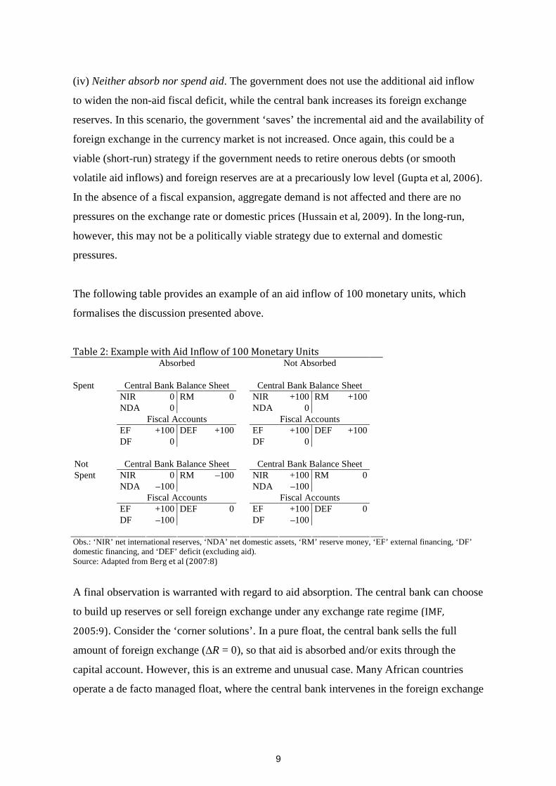
(iv) Neither absorb nor spend aid. The government does not use the additional aid inflow

to widen the non-aid fiscal deficit, while the central bank increases its foreign exchange

reserves. In this scenario, the government ‘saves’ the incremental aid and the availability of

foreign exchange in the currency market is not increased. Once again, this could be a

viable (short-run) strategy if the government needs to retire onerous debts (or smooth

volatile aid inflows) and foreign reserves are at a precariously low level (Gupta et al, 2006).

In the absence of a fiscal expansion, aggregate demand is not affected and there are no

pressures on the exchange rate or domestic prices (Hussain et al, 2009). In the long-run,

however, this may not be a politically viable strategy due to external and domestic

pressures.

The following table provides an example of an aid inflow of 100 monetary units, which

formalises the discussion presented above.

Table 2: Example with Aid Inflow of 100 Monetary UnitsAbsorbed Not Absorbed

Spent Central Bank Balance Sheet Central Bank Balance SheetNIR 0 RM 0 NIR +100 RM +100NDA 0 NDA 0

Fiscal Accounts Fiscal AccountsEF +100 DEF +100 EF +100 DEF +100DF 0 DF 0

Not Central Bank Balance Sheet Central Bank Balance SheetSpent NIR 0 RM –100 NIR +100 RM 0

NDA –100 NDA –100Fiscal Accounts Fiscal Accounts

EF +100 DEF 0 EF +100 DEF 0DF –100 DF –100

Obs.: ‘NIR’ net international reserves, ‘NDA’ net domestic assets, ‘RM’ reserve money, ‘EF’ external financing, ‘DF’domestic financing, and ‘DEF’ deficit (excluding aid).Source: Adapted from Berg et al (2007:8)

A final observation is warranted with regard to aid absorption. The central bank can choose

to build up reserves or sell foreign exchange under any exchange rate regime (IMF,

2005:9). Consider the ‘corner solutions’. In a pure float, the central bank sells the full

amount of foreign exchange (∆R = 0), so that aid is absorbed and/or exits through the

capital account. However, this is an extreme and unusual case. Many African countries

operate a de facto managed float, where the central bank intervenes in the foreign exchange

10

market (e.g. accumulation of reserves) due to a ‘fear of floating’ (Calvo and Reinhart,

2002:388). For this reason, any combination of the three uses of aid would be possible. In a

fixed regime (e.g. CFA Franc Zone), the central bank accumulates the foreign exchange to

defend the fixed peg (∆R = ∆Aid) and none of the aid is absorbed. However, as the fiscal

stimulus contributes to higher demand for net imports the central bank may decide to sell

the foreign exchange to defend the peg – nominal depreciation pressures in ‘spend and not

absorb’ – which may lead to full absorption (IMF, 2005:9). Hence, one could argue that

while the exchange rate regime may condition the short-term response to aid, in the long-

run, countries with different exchange rate and monetary frameworks may adopt similar

policy responses. This assumption supports the main empirical framework proposed by this

paper (pooled mean group estimator), which constrains the long-run impacts to be identical

across countries but allows for short-run heterogeneous effects.

The aim of this section was to briefly introduce the analytical framework and concepts that

are going to be used in the empirical assessment. The next section presents the empirical

findings of the relevant literature.

Empirical Results

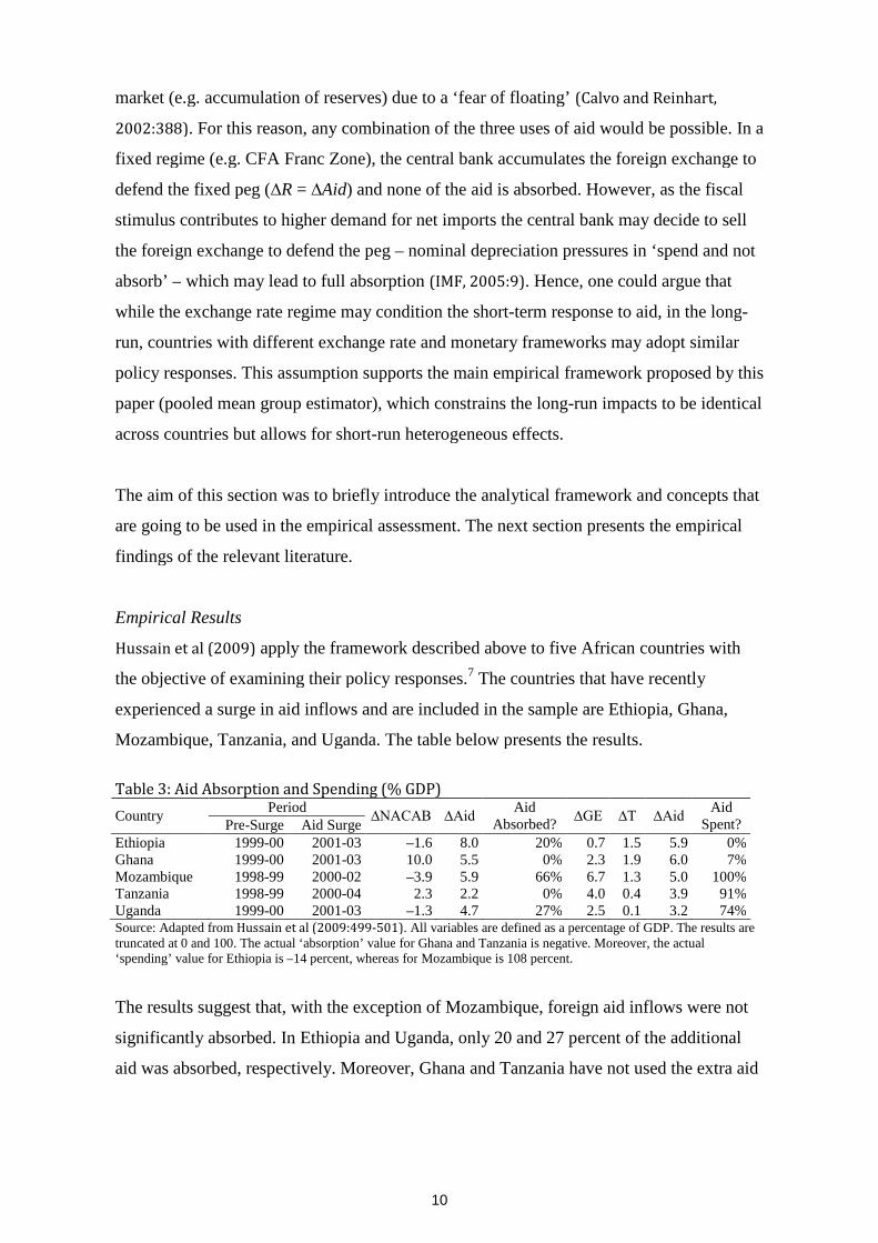
Hussain et al (2009) apply the framework described above to five African countries with

the objective of examining their policy responses.7 The countries that have recently

experienced a surge in aid inflows and are included in the sample are Ethiopia, Ghana,

Mozambique, Tanzania, and Uganda. The table below presents the results.

Table 3: Aid Absorption and Spending (% GDP)Period

CountryPre-Surge Aid Surge

∆NACAB ∆AidAid

Absorbed?∆GE ∆T ∆Aid

AidSpent?

Ethiopia 1999-00 2001-03 –1.6 8.0 20% 0.7 1.5 5.9 0%Ghana 1999-00 2001-03 10.0 5.5 0% 2.3 1.9 6.0 7%Mozambique 1998-99 2000-02 –3.9 5.9 66% 6.7 1.3 5.0 100%Tanzania 1998-99 2000-04 2.3 2.2 0% 4.0 0.4 3.9 91%Uganda 1999-00 2001-03 –1.3 4.7 27% 2.5 0.1 3.2 74%Source: Adapted from Hussain et al (2009:499-501). All variables are defined as a percentage of GDP. The results aretruncated at 0 and 100. The actual ‘absorption’ value for Ghana and Tanzania is negative. Moreover, the actual‘spending’ value for Ethiopia is –14 percent, whereas for Mozambique is 108 percent.

The results suggest that, with the exception of Mozambique, foreign aid inflows were not

significantly absorbed. In Ethiopia and Uganda, only 20 and 27 percent of the additional

aid was absorbed, respectively. Moreover, Ghana and Tanzania have not used the extra aid

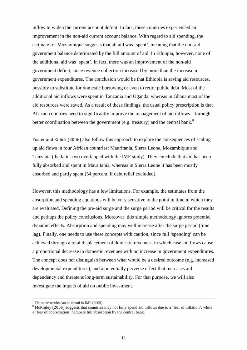
11

inflow to widen the current account deficit. In fact, these countries experienced an

improvement in the non-aid current account balance. With regard to aid spending, the

estimate for Mozambique suggests that all aid was ‘spent’, meaning that the non-aid

government balance deteriorated by the full amount of aid. In Ethiopia, however, none of

the additional aid was ‘spent’. In fact, there was an improvement of the non-aid

government deficit, since revenue collection increased by more than the increase in

government expenditures. The conclusion would be that Ethiopia is saving aid resources,

possibly to substitute for domestic borrowing or even to retire public debt. Most of the

additional aid inflows were spent in Tanzania and Uganda, whereas in Ghana most of the

aid resources were saved. As a result of these findings, the usual policy prescription is that

African countries need to significantly improve the management of aid inflows – through

better coordination between the government (e.g. treasury) and the central bank.8

Foster and Killick (2006) also follow this approach to explore the consequences of scaling

up aid flows in four African countries: Mauritania, Sierra Leone, Mozambique and

Tanzania (the latter two overlapped with the IMF study). They conclude that aid has been

fully absorbed and spent in Mauritania, whereas in Sierra Leone it has been mostly

absorbed and partly spent (54 percent, if debt relief excluded).

However, this methodology has a few limitations. For example, the estimates from the

absorption and spending equations will be very sensitive to the point in time in which they

are evaluated. Defining the pre-aid surge and the surge period will be critical for the results

and perhaps the policy conclusions. Moreover, this simple methodology ignores potential

dynamic effects. Absorption and spending may well increase after the surge period (time

lag). Finally, one needs to use these concepts with caution, since full ‘spending’ can be

achieved through a total displacement of domestic revenues, in which case aid flows cause

a proportional decrease in domestic revenues with no increase in government expenditures.

The concept does not distinguish between what would be a desired outcome (e.g. increased

developmental expenditures), and a potentially perverse effect that increases aid

dependency and threatens long-term sustainability. For that purpose, we will also

investigate the impact of aid on public investment.

7 The same results can be found in IMF (2005).8 McKinley (2005) suggests that countries may not fully spend aid inflows due to a ‘fear of inflation’, whilea ‘fear of appreciation’ hampers full absorption by the central bank.

12

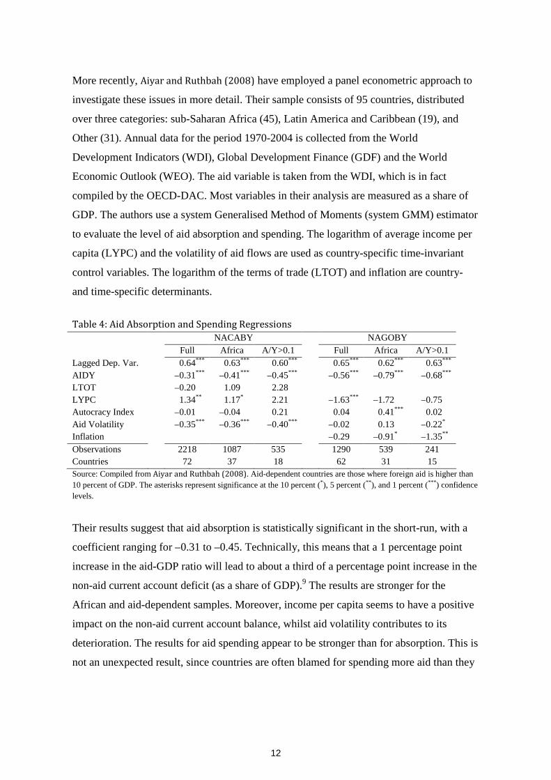
More recently, Aiyar and Ruthbah (2008) have employed a panel econometric approach to

investigate these issues in more detail. Their sample consists of 95 countries, distributed

over three categories: sub-Saharan Africa (45), Latin America and Caribbean (19), and

Other (31). Annual data for the period 1970-2004 is collected from the World

Development Indicators (WDI), Global Development Finance (GDF) and the World

Economic Outlook (WEO). The aid variable is taken from the WDI, which is in fact

compiled by the OECD-DAC. Most variables in their analysis are measured as a share of

GDP. The authors use a system Generalised Method of Moments (system GMM) estimator

to evaluate the level of aid absorption and spending. The logarithm of average income per

capita (LYPC) and the volatility of aid flows are used as country-specific time-invariant

control variables. The logarithm of the terms of trade (LTOT) and inflation are country-

and time-specific determinants.

Table 4: Aid Absorption and Spending Regressions

NACABY NAGOBY

Full Africa A/Y>0.1 Full Africa A/Y>0.1

Lagged Dep. Var. 0.64*** 0.63*** 0.60*** 0.65*** 0.62*** 0.63***

AIDY –0.31*** –0.41*** –0.45*** –0.56*** –0.79*** –0.68***

LTOT –0.20*** 1.09*** 2.28***

LYPC 1.34*** 1.17*** 2.21*** –1.63*** –1.72*** –0.75***

Autocracy Index –0.01*** –0.04*** 0.21*** 0.04*** 0.41*** 0.02***

Aid Volatility –0.35*** –0.36*** –0.40*** –0.02*** 0.13*** –0.22***

Inflation –0.29*** –0.91*** –1.35***

Observations 2218 1087 535 1290 539 241

Countries 72 37 18 62 31 15

Source: Compiled from Aiyar and Ruthbah (2008). Aid-dependent countries are those where foreign aid is higher than

10 percent of GDP. The asterisks represent significance at the 10 percent (*), 5 percent (**), and 1 percent (***) confidence

levels.

Their results suggest that aid absorption is statistically significant in the short-run, with a

coefficient ranging for –0.31 to –0.45. Technically, this means that a 1 percentage point

increase in the aid-GDP ratio will lead to about a third of a percentage point increase in the

non-aid current account deficit (as a share of GDP).9 The results are stronger for the

African and aid-dependent samples. Moreover, income per capita seems to have a positive

impact on the non-aid current account balance, whilst aid volatility contributes to its

deterioration. The results for aid spending appear to be stronger than for absorption. This is

not an unexpected result, since countries are often blamed for spending more aid than they

13

absorb (no real resource transfer). In this case, the impact for Africa appears to be stronger

than for aid-dependent countries. Finally, the autocracy index appears to improve the

government balance while inflation has the opposite effect. For aid-dependent countries,

only inflation and aid volatility seem to be statistically significant.

To complement their analysis, Aiyar and Ruthbah (2008) also estimate the impact of

foreign aid inflows on the accumulation of international reserves and total domestic

investment. Their results suggest that aid has no impact on the accumulation of foreign

reserves. Moreover, income per capita and the terms of trade may have a positive impact.

Finally, foreign aid contributes to a modest increase in total domestic investment, when

controlled for public investment.

Table 5: International Reserves and Investment RegressionsdRY INVY

Full Africa A/Y>0.1 Full Africa A/Y>0.1Lagged Dep. Var. 0.02* 0.04* –0.05** 0.48*** 0.43*** 0.42***

AIDY 0.05* 0.01* 0.06** 0.14*** 0.15*** 0.19***

L(ToT) 0.54* 0.61* 0.52** –1.79*** –1.70*** –0.59***

L(YPC avg) 0.37* 0.52* 0.28** 0.60*** 0.39*** 0.16***

Autocracy Index –0.02* 0.04* 0.04** –0.01*** 0.08*** –0.04***

Aid Volatility –0.05* 0.01* –0.02** 0.20*** 0.23*** 0.25***

INVPY 0.54*** 0.60*** 0.68***

Observations 2073 1007 485 1813 888 389Countries 72 37 18 72 37 18Source: Compiled from Aiyar and Ruthbah (2008). The asterisks represent significance at the 10 percent (*), 5 percent(**), and 1 percent (***) confidence levels.

The table below summarises the short- and long-run effects of an increase in aid inflows.

The long-run coefficients are obtained by dividing the estimated (short-run) coefficient by

1 minus the coefficient of the lagged dependent variable. The long-run results indicate that

aid has a more than proportional effect on the non-aid current account balance and the non-

aid government balance. Although there is no impact on the accumulation of international

reserves, aid seems to contribute to a modest increase in total investment. Finally, the

authors argue that the unabsorbed aid is leaving the countries through the capital account.

This study will revisit the empirical evidence on aid absorption and spending, with a

special focus on low-income countries in Africa. For that purpose we compiled data from

several international sources and constructed a new (balanced) panel dataset. Contrary to

9 The authors interpret these results differently. For the first column they suggest that (in the short-run) “about 30 centsout of every dollar is absorbed” (Aiyar and Ruthbah, 2008:10).

14

what is common practice in this field of research, we do not use the OECD-DAC’s dataset

on aid flows, but instead collect consistent aid data as reported by the recipients.

Furthermore, we use alternative panel data methodologies, which we argue are more

appropriate to deal with this type of macroeconomic dataset.

Table 6: Impact of a 1 percentage point increase in the Aid-GDP RatioFull Sample Africa A/Y > 0.1

Short-Run Long-Run Short-Run Long-Run Short-Run Long-RunAbsorption 0.30*** 0.83*** 0.41*** 1.11*** 0.45*** 1.13***

Spending 0.56*** 1.60*** 0.79*** 2.14*** 0.68*** 1.48***

Reserves 0.05*** 0.05*** 0.01*** 0.00*** 0.06*** 0.00***

Investment 0.14*** 0.26*** 0.15*** 0.26*** 0.19*** 0.33***

Source: Aiyar and Ruthbah (2008:13) for full sample and author’s calculations for remaining samples. The asterisksrepresent significance at the 10 percent (*), 5 percent (**), and 1 percent (***) confidence levels.

3. Methodology

This paper uses (linear) panel data regression methods to evaluate how African countries

have managed foreign aid inflows. Panel data is a special case of pooled time-series cross-

section, in which the same cross-section (e.g. individual) is surveyed over time. In this

paper, the cross-section includes African countries, for which annual observations of a

number of variables were collected. Baltagi (2008:6-11) provides a good summary of the

advantages and disadvantages of using panel data. Here we focus on the aspects that

contrast macro panels to time series regressions. Some of the advantages include: (i)

controlling for individual heterogeneity;10 (ii) more informative data, variability, degrees of

freedom and efficiency, as well as less collinearity among the variables; (iii) allowing the

construction and testing of more complicated behavioural models; and (iv) panel unit root

tests that have more power and have standard asymptotic distributions.

In terms of its limitations, the most serious are: (i) the ‘poolability’ (homogeneity)

assumption, although there are formal tests to evaluate its validity; (ii) potential cross-

sectional dependence, which complicates the analysis; (iii) some tests and methods require

balanced panels; and (iii) cross-country data consistency. With these features in mind, we

now proceed to the presentation of two important methodological approaches – dynamic

panel data (DPD) methods and cointegration analysis.

10 Unobserved heterogeneity or time-invariant variables that are correlated with explanatory variables (such as history,institutions and political regimes) may cause omitted variable bias in time series regressions.

15

3.1 Dynamic Panel Data

Economic relationships often incorporate some degree of dynamic behaviour. To capture

this feature, dynamic panel data (DPD) models – which include a lagged dependent

variable – are usually considered (Baltagi, 2008:147):

where δ is a scalar, xit is a 1 x k vector of explanatory variables and β is a k x 1 vector of

coefficients. For the purpose of illustration, assume that uit is a one-way error component

model:

where μi ~ IID(0,2μ) and vit ~ IID(0,2

v) independent of each other and among themselves.

This DPD model is characterised by two sources of persistence over time: (i)

autocorrelation due to the lagged dependent variable; and (ii) individual effects capturing

country heterogeneity (Baltagi, 2008:147). Estimation of DPD models raises several

problems in both fixed- and random-effects. For example, the lagged dependent variable is

correlated with the disturbance term (since yi,t–1 is a function of μi), even if the vit is not

serially correlated (Greene, 2003:307). The OLS estimator is biased and inconsistent in

finite samples, especially if T is small. In fact, the coefficients of the explanatory variables

will be subject to a downward bias in absolute terms (i.e. biased towards zero). Even for

T=30 the fixed-effects (FE) estimator can present a significant bias (Baltagi, 2008:148).

The solution is thus to use instrumental variables (IV) regressions or generalised method of

moments (GMM) estimators (Greene, 2003:308-14).

Arellano and Bond (1991) developed one- and two-step GMM estimators for dynamic

panels (‘difference GMM’). They obtain additional instruments by using orthogonality

conditions between the lagged dependent variables and the disturbance terms. The

difference GMM does not require any prior knowledge of the initial conditions or even the

distribution of vi and μi. However, if the dependent variable is very persistent (close to a

random walk), then the lagged levels are poor instruments for first-differences and

difference GMM performs poorly. Blundell and Bond (1998) develop a ‘system GMM’

16

estimator for DPD models to solve the problem of ‘weak instruments’. The Blundell-Bond

estimator combines moment conditions for the model in first-differences with those for the

model in levels. The procedure uses lagged differences of yit as instruments for the

equation in levels and lagged levels of yit as instruments for the equation in first-

differences. Moreover, it requires a stationary restriction on the initial conditions process

(Baltagi, 2008:161). The validity of the moment conditions imposed are usually assessed by

a test of over-identifying restrictions (either Hansen’s or Sargan’s).

The main advantages of these GMM estimators relate to their perceived robustness to

heteroscedasticity and non-normality of the disturbances. Moreover, the use of

instrumental variables helps address biases arising from reverse causality. Nonetheless,

there are some remaining concerns about the efficiency of such methods. The violation of

moment conditions (e.g. presence of non-stationarity), will yield inconsistent estimates.

Moreover, Roodman (2009) argues that the number (and quality) of instruments generated

by difference and system GMM methods can affect the asymptotic properties of the

estimators and specification tests. In samples with large T, instrument proliferation can be

particularly serious, inducing two main types of problems: (i) overfitting endogenous

variables; and (ii) imprecise estimates of the optimal weighting matrix. Greene (2003:307)

provides another strong criticism. He argues that introducing a lagged dependent variable

to an otherwise long-run (static) equation will significantly change its interpretation,

especially for the independent variables. In the case of a DPD model, the coefficient on xit

merely represents the effect of new information, rather than the full set of information that

influences yit. Finally, it is often argued that while DPD methods are appropriate for panels

with a small T, but when T is sufficiently large other methods should be preferred. Hence,

we now turn to panel data methods that were specifically developed for ‘long’ panels.

3.2 Panel Cointegration

Traditional panel data econometrics rests on micro panels that usually include thousands of

households or hundreds of firms (large N), which are tracked over a few survey rounds

(small T). This study, however, uses macroeconomic variables that are collected for several

African countries over a significant number of years. The use of panel datasets with these

characteristics – large N and large T – presents new challenges to researchers. Panels with

a significant temporal dimension are subject to spurious relationships, especially since

17

macroeconomic variables are often characterised by non-stationarity. According to Baltagi

(2008:273), the accumulation of observations through time generated two strands of ideas:

(i) the use of heterogeneous regressions (one for each country) instead of accepting

coefficient homogeneity (implicit in pooled regressions), e.g. Pesaran et al (1999); and (ii)

the extension of time series methods (estimators and tests) to panels in order to deal with

non-stationarity and cointegration, e.g. Kao and Chiang (2000) and Pedroni (2000).11 We

will pursue both strategies in this paper.

Cointegration analysis in a panel data setting entails similar steps to those usually

employed in time series analysis: (i) unit root testing; (ii) cointegration testing; and (iii)

estimation of long-run relationships. We take these in turn.

Unit Root Tests

The first step requires an analysis of the stationarity properties of the variables. Panel unit

root tests have become a fast-growing area of research in econometrics with a view to

improving the perceived low power of individual unit root tests – particularly in small

samples. These tests are often grouped into two main categories: (i) first-generation tests,

which assume cross-sectional independence – e.g. Levin et al (2002), Im et al (2003),

Maddala and Wu (1999), and Choi (2001); and (ii) second-generation tests, which explicitly

allow for some form of cross-sectional dependence – e.g. Pesaran (2007). As a starting

point, consider the following autoregressive (AR) process for panel data:

where ρi is the AR coefficient and the error term uit is assumed to be independent and

identically distributed (i.i.d.). Moreover, Zit includes individual deterministic effects, such

as constants (‘fixed effects’) and linear time trends, which capture cross-sectional

heterogeneity.

Levin et al (2002)12 propose a test (LLC) that can be seen as a panel extension of the

augmented Dickey-Fuller (ADF) test:

11 Moreover, the estimators for panel cointegrated models and related statistical tests are often found to have differentasymptotic properties from their time series counterparts (Baltagi, 2008:298). An important contribution is Phillips andMoon (1999, 2000), who analyse the limiting distribution of double indexed integrated processes.12 Originally published in 1992 and one of the first panel unit root tests in the literature.

18

Since the lag length of the differenced terms (pi) is unknown, Levin et al (2002:5-7) suggest

the following three-step procedure: (i) carry out separate ADF regressions for each

individual and generate two orthogonalised residuals;13 (ii) estimate the ratio of long-run to

short-run innovation standard deviation for each individual; (iii) compute the pooled t-

statistics, with the average number of observations per individual and average lag length.

In this test, the associated AR coefficient is constrained to be homogenous across

individuals (i.e. αi = α for all i). Hence, the null hypothesis assumes a common unit root

(H0: α = ρ – 1 = 0) against the alternative hypothesis that each time series is stationary (H1:

α < 0). The authors show that the pooled t-statistic has a limiting normal distribution under

the null hypothesis. This test is often recommended for moderate sized panels, especially

for N>10 and T>25.

Im et al (2003)14 extend the LLC test by allowing heterogeneity on the AR coefficient. In

practice, the test entails the estimation of individual ADF regressions, and then combining

this information to perform a panel unit root test. This approach allows for different

specifications of the coefficients (αi for each cross-section), the residual variance and lag-

length (Asteriou and Hall, 2007:368). The authors propose a t-bar statistic, based on the

average of the individual unit root (ADF) test statistics. This statistic evaluates whether the

coefficient α is non-stationary across all individuals (H0: αi = 0 for all i), against the

alternative hypothesis that at least a fraction of the series is stationary (H1: αi < 0 for at least

one i). Both LLC and IPS tests require N to be small enough relative to T, whilst the LLC

test also requires a strongly balanced panel (Baltagi, 2008:280).

Breitung (2000) uses Monte Carlo experiments to show that the power of the LLC and IPS

tests statistics is sensitive to the specification of the deterministic components, such as the

inclusion of individual specific trends (Baltagi, 2008:280). He proposes a test statistic based

on modifications to the LLC steps to overcome these difficulties. Breitung’s test statistic

13 Here, the lag order of the differenced terms (pi) is allowed to vary across individuals and is usually determined by a lagselection criterion (to correct for serial correlation).14 The IPS test was originally published in 1997.

19

assumes a common unit root process and is also shown to be asymptotically distributed as

a standard normal. The test is often suggested for samples of around N=20 and T=30.

Maddala and Wu (1999:637) and Choi (2001) suggest the use of nonparametric Fisher tests.

The main feature of these tests is that they combine the probability limit values (p-values)

of unit root tests from each cross-section rather than average test statistics. Fisher tests are

usually implemented using individual ADF or Phillips-Perron unit root tests, and their

asymptotic distribution follows a chi-square (P-test).15Choi (2001) also proposes an

alternative Fischer-type statistic that follows a standard normal distribution (Z-test). Both

IPS and Fischer-type tests combine information of individual unit root tests, but simulation

studies suggest that Fischer tests have better power properties than the IPS test. The

disadvantage of Fischer-type tests relates to the need to derive p-values through Monte

Carlo simulations.

Hadri (2000) proposes a residual-based Lagrange multiplier (LM) test, which is in fact a

panel generalisation of the KPSS test (Baltagi, 2008:282). The test uses the residuals from

individual OLS regressions of yit on deterministic components (constant and trend) to

compute the LM statistic. This test also differs from the previous in the sense that it is a

stationarity test. The null hypothesis assumes no unit root in any of the time series (all

panels stationary), against the alternative of non-stationarity for, at least, some cross-

sections.

The main drawback of the first-generation tests described above relates to the assumption

that the data is independent and identically distributed (i.i.d.) across individuals (cross-

section independence). In practice, this means that the movements of a given variable

through time are independent across countries. This restrictive assumption has often been

challenged by empirical studies, and it should be evaluated on a case-by-case basis.16 Some

cross-sectional dependence tests include Pesaran (2004) and a Breusch-Pagan LM statistic

(for T>N). Banerjee et al (2005) show that in the presence of cross-section dependence,

first-generation tests tend to have serious size distortions and therefore perform poorly.

15 Maddala and Wu (1999:645) also suggest a bootstrap procedure to account for cross-sectional dependence, but sizedistortions are only decreased rather than eliminated.16 Levin et al (2002) suggest ‘demeaning’ the data in order to attenuate the biases caused by the presence of cross-sectional dependence, which involves subtracting cross-sectional averages (for each time period) from the series beforethe use of unit root tests. Nonetheless, this procedure cannot ensure the successful elimination of the bias.

20

This often leads to the over-rejection of the null hypothesis (unit root) when the sources of

non-stationarity are common across individuals.

These findings led to the development of unit root tests for panels with cross-sectional

dependence (second-generation tests). Pesaran (2007) suggests a simple method to remove

the influence of cross-sectional dependence, which involves augmenting standard ADF

regressions with the cross-section averages of lagged levels and first-differences of the

individual series. These individual cross-sectionally augmented Dickey-Fuller (CADF)

statistics (or the corresponding p-values) can then be used to develop modified versions of

standard panel unit root tests – such as IPS’s t-bar, Maddala and Wu’s P, or Choi’s Z. The

tests are applicable for both when N>T and T>N, and are shown to have good size and

power properties, even when N and T are relatively small (e.g. 10). However, the t-bar

statistic (CIPS) can only be computed for balanced panels. For unbalanced panels, the

modified Z test can be reported.

Table 7: Characteristics of Unit Root TestsTest Null Alternative

HypothesisDeterministicComponents

AutocorrelationCorrection

Cross-SectionDependence

UnbalancedPanel (Gaps)

LLC UR No UR None, F, T Lags demean No ( – )Breitung UR No UR F, T Lags robust1 No ( – )IPS UR Some CS without UR None, F, T Lags demean Yes (No)Fisher UR Some CS without UR None, F, T Lags/Kernel demean Yes (Yes)Hadri No UR Some CS with UR F, T Kernel robust1 No ( – )Pesaran UR Some CS without UR F, T Lags robust Yes (No)Obs.: ‘UR’ unit root, ‘CS’ cross-sections, ‘None’ no exogenous variables, ‘F’ fixed effect, ‘T’ individual effect andindividual trend. 1 Stata’s ‘xtunitroot’ command computes robust versions that account for cross-sectional dependence.Source: Compiled from QMS (2007:110, corrected) and Stata’s ‘xtunitroot’ command help.

Cointegration Tests

The panel unit root tests proposed above aim to assess the order of integration of the

variables. If the main variables are found to be integrated of order one, then we should use

panel cointegration tests to address the non-stationarity of the series. As before, some of

these tests were developed as extensions of earlier tests for time series data.

Pedroni (1999, 2004:604) provides cointegration tests for heterogeneous panels based on

the two-step cointegration approach of Engle and Granger (1987). Pedroni uses the

residuals from the static (long-run) regression and constructs seven panel cointegration test

statistics: four of them are based on pooling (within-dimension or ‘panel statistics test’),

21

which assumes homogeneity of the AR term, whilst the remaining are less restrictive

(between-dimension or ‘group statistics test’) as they allow for heterogeneity of the AR

term. The assumption has implications on the computation of the second step and the

specification of the alternative hypothesis. The v-statistic is analogous to the long-run

variance ratio statistic for time series, while the rho-statistic is equivalent to the semi-

parametric ‘rho’ statistic of Phillips and Perron (1988). The other two are panel extensions

of the (non-parametric) Phillips-Perron and (parametric) ADF t-statistics, respectively.

These tests allow for heterogeneous slope coefficients, fixed effects and individual specific

deterministic trends, but are only valid if the variables are I(1). Pedroni (1999) derived

critical values for the null hypothesis of no cointegration.

Kao (1999) proposes residual-based DF and ADF tests similar to Pedroni’s, but specifies

the initial regression with individual intercepts (‘fixed effects’), no deterministic trend and

homogeneous regression coefficients. Kao’s tests converge to a standard normal

distribution by sequential limit theory (Baltagi, 2008:293). Both Kao and Pedroni tests

assume the presence of a single cointegrating vector, although Pedroni’s test allows it to be

heterogeneous across individuals.

Maddala and Wu (1999) propose a Fisher cointegration test based on the multivariate

framework of Johansen (1988). They suggest combining the p-values of individual

(system-based) cointegration tests in order to obtain a panel test statistic. Moreover,

Larsson et al (2001) suggest a likelihood ratio statistic (LR-bar) that averages individual

rank trace statistics. However, the authors find that the test requires a large number of

temporal observations. Both of these tests allow for multiple cointegrating vectors in each

cross-section.

Westerlund (2007) suggests four cointegration tests that are an extension of Banerjee et al

(1998). These tests are based on structural rather than residual dynamics and allow for a

large degree of heterogeneity (e.g. individual specific short-run dynamics, intercepts, linear

trends and slope parameters).17 All variables are assumed to be I(1). Moreover,

bootstrapping provides robust critical values in cases of cross-section dependence. The

17 Westerlund (2007:710) argues that residual-based cointegration tests require the long-run cointegration vector inlevels to equal the short-run adjustment process in differences – also known as ‘common factor restrictions’. The trade-off is the assumption of weak exogeneity that ECM-based tests depend upon.

22

tests assess the null hypothesis that the error correction term in a conditional ECM is zero –

i.e. no cointegration (Baltagi, 2008:306).

Banerjee et al (2004) argue that although these tests allow for cross-sectional dependence

(via the effects of short-run dynamics), they do not consider long-run dependence, induced

by cross-sectional cointegration. The authors demonstrate that in that case, panel

cointegration tests may be significantly oversized (Baltagi, 2008:302-3). Moreover, most

cointegration tests may be misleading in the presence of stationary data, as they require all

data to be I(1).

Estimation of the Long-Run

A complementary issue relates to the efficient estimation of long-run economic

relationships. In the presence of cointegrating non-stationary variables, one would like to

be able to efficiently estimate and test the relevant cointegrating vectors. For that purpose,

a number of panel estimators have been suggested in the literature. Once again, most of

them are developed as extensions of well-known time series methods. An important

difference is that the panel OLS estimator of the (long-run) static regression model,

contrary to its time series counterpart, is inconsistent (Baltagi, 2008:299).

Kao and Chiang (2000) propose a panel dynamic OLS estimator (DOLS) which is a

generalisation of the method originally proposed by Saikkonen (1991) and Stock and

Watson (1993) for time series regressions. The regression equation is:

where Xit is a vector of explanatory variables, the estimated long-run impact, q the

number of leads and lags of the first-differenced data, and cij the associated parameters.

The estimator assumes cross-sectional independence and is asymptotically normally

distributed. The authors provide Monte Carlo results suggesting that the finite-sample

23

properties of the DOLS estimator are superior to both fully-modified OLS (FMOLS)18 and

OLS estimators.

Pesaran et al (1999) suggest a (maximum-likelihood) pooled mean group (PMG) estimator

for dynamic heterogeneous panels. The procedure fits an autoregressive distributed lag

(ARDL) model to the data, which can be re-specified as an error correction equation to

facilitate economic interpretation. Consider the following error correction representation of

an ARDL(p, q, q,…, q) model:

where X is a vector of explanatory variables, i contains information about the long-run

impacts, i is the error correction term (due to normalisation), and δij incorporates short-run

information. The PMG can be seen as an intermediate procedure, somewhere between the

mean group (MG) estimator and the dynamic fixed-effects (DFE) approach.19 The MG

estimator is obtained by estimating N independent regressions and then averaging the

(unweighted) coefficients, whilst the DFE requires pooling the data and assuming that the

slope coefficients and error variances are identical. The PMG, however, restricts the long-

run coefficients to be same (=i for all i), but allows the short-run coefficients and error

variances to vary across countries (Pesaran et al, 1999:621). This approach can be used

whether the regressors are I(0) or I(1) (Pesaran et al, 1999:625).

4. Data

The data used in this paper was collected from the International Monetary Fund’s (IMF)

Balance of Payments Statistics (BoPS) and the World Bank’s Africa Database.

Complementary sources included the United Nations’ National Accounts Main Aggregates

Database, the IMF’s World Economic Outlook (WEO), and the World Bank’s World

Development Indicators (WDI). There was a significant effort to construct a balanced

panel for all 53 African countries covering the period 1970-2007. However, data for 1970-

1979 is scarce for many countries, whereas data for 2006-2007 is usually based on

18 The panel FMOLS estimator developed by Phillips and Moon (1999) and Pedroni (2000) is a generalisation of theestimator proposed by Phillips and Hansen (1990).19 A further estimation alternative would be Zellner’s seemingly unrelated regression (SUR), but this procedure requiresthat N is significantly smaller than T, which unfortunately is not our case. Moreover, Pesaran et al (1999:626) arguethat Swamy’s static random coefficient model is asymptotically equivalent to the MG estimator.

24

estimates or projections. Moreover, data on aid flows for 2006 often contains outliers due

to very large debt relief grants, which cannot be satisfactorily expunged. Hence, we have

built a balanced panel for 1980-2005 for the macroeconomic variables, while for the fiscal

variables we have a balanced panel for 1990-2005. It should be noted that our aid variables

only include grants, due to the lack of data on concessional foreign loans. Nonetheless,

there is a strong argument to separate these since aid grants and aid loans often have

significantly different economic impacts.20 Finally, seven countries had to be excluded

from the initial sample. These countries either reached independence only in the 1990s

(Eritrea and Namibia) or lack reliable data (Congo DR, Djibouti, Liberia, Somalia and

Zimbabwe).

The list of variables includes:

NACABY Non-Aid Current Account Balance (% GDP)

AIDBOPY Aid Grants (% GDP), as reported by the Balance of Payments Statistics

LTOT Logarithm of the Terms of Trade

DRY Change in International Reserves (% GDP)

NAGOBY Non-Aid Government Overall Balance (% GDP)

AIDGOVY Aid Grants (% GDP), as reported by the World Bank’s Africa Database

INF Inflation Rate (CPI, percentage change)

INVGY Gross Public Fixed Capital Formation (% GDP)

BORY Domestic Financing (% GDP)

The following graphs provide pair-wise plots of the main variables of interest. The full

sample of African countries is utilised, as well as a sub-sample incorporating low-income

countries (LICs) only.21 The plots confirm the strong negative correlation between foreign

aid and the macroeconomic and fiscal balances. This suggests that aid inflows are used, at

least to a certain extent, to increase the (non-aid) current account and budget deficits.

However, there is an important concern arising from the observation of these graphs. It

appears that richer countries may potentially distort the analysis. This is because middle-

income countries tend to be less aid-dependent, and therefore the relationship between aid

inflows and other economic variables can be significantly weaker. The inclusion of these

countries may thus affect the magnitude and significance of the estimated coefficients,

20 In practice, we allow ‘aid loans’ to remain lumped with foreign non-concessional loans.21 As defined by the World Bank (July 2009).

25

leading us to believe that aid absorption and spending is lower than desired. Further plots

lead to similar conclusions for reserve accumulation and public investment. Finally, some

of the richer countries are (at times) net ‘donors’, which further complicates the analysis.

Figure 1: Non-Aid Current Account Balances and Foreign Aid

-15

0-1

00

-50

05

0

0 20 40 60 0 20 40 60

Non-LIC LIC

NA

CA

BY

AIDBOPY

Obs.: Excludes Lesotho (LSO)

Figure 2: Non-Aid Government Balances and Foreign Aid

-100

-50

050

0 10 20 30 0 10 20 30

Non-LIC LIC

NA

GO

BY

AIDGOVY

Obs.: Excludes the Republic of Congo (COG)

The table below presents pair-wise correlations between the main variables of interest. The

results corroborate the decision to exclude middle-income countries from the analysis, as

for both macroeconomic and fiscal dimensions the (negative) correlations of the non-aid

balances with foreign aid inflows are significantly stronger for low-income countries.

For the reasons presented above, this study will continue the analysis for the 25 African

low-income countries in the sample. The following tables present basic statistics on the

26

main variables.22 As expected, both NACABY and NAGOBY have negative means, with

fairly low maximums (surpluses). This highlights the importance of aid inflows in

balancing these accounts. The average for AIDBOPY is higher than that for AIDGOVY,

probably reflecting the presence of ‘off-budgets’ – i.e. aid flows not recorded in the budget,

perhaps because they are implemented by the donor. BORY has a positive (but low) mean

value.

Table 8: CorrelationsALL LIC

1980-2005 NACABY

AIDBOPY NACABY AIDBOPY

NACABY 1.00 1.00AIDBOPY –0.56 1.00 –0.63 1.00

1990-2005 NAGOBY

AIDGOVY

NAGOBY AIDGOVY

NAGOBY 1.00 1.00AIDGOVY –0.72 1.00 –0.83 1.00

Table 9: Basic Statistics for Macroeconomic Variables (1980-2005)Obs. Mean SD Min Max

NACABY 650 –12.2 9.6 –59.7 11.1AIDBOPY 650 7.7 6.5 0.2 46.5LTOT 650 4.7 0.4 2.7 5.8DRY 650 –0.5 3.1 –16.0 34.9

Table 10: Basic Statistics for Fiscal Variables (1990-2005)Obs. Mean SD Min Max

NAGOBY 400 –11.6 7.4 –53.0 1.9AIDGOVY 400 4.9 3.5 0.2 18.9INF 400 13.4 20.5 –10.9 183.3INVGY 400 7.6 3.8 1.4 32.2BORY 400 0.8 2.5 –6.7 13.8

5. Empirical Results

This section undertakes a comprehensive econometric exercise to evaluate the uses of

foreign aid in Africa’s low-income countries. The sample for the macroeconomic

specification (absorption) runs from 1980 to 2005, while the fiscal regressions (spending)

cover the period 1990-2005. The previous section has demonstrated that the inclusion of

middle-income countries – for whom foreign aid plays a much lesser role – can

significantly distort the analysis. Hence, the sample in this section is restricted to the 25

African low-income countries in our sample.

22 Not surprisingly, the full sample shows lower absolute averages and higher standard deviations for the aid variables.

27

Since we are dealing with macroeconomic and fiscal variables that are often found to be

non-stationary, we first undertake panel unit root tests to evaluate their order of integration.

The results provide evidence that at least some of the variables are non-stationary. We then

apply panel cointegration tests to assess whether there are long-run relationships amongst

the variables of interest. Finally, long-run relations are estimated through appropriate and

efficient methods.

5.1 Panel Unit Roots

We start with the application of panel unit root tests. A detailed description of the specific

characteristics of each test was provided in a previous section. All test specifications

include a deterministic time trend. In the LLC, IPS and Fisher-type tests, cross-sectional

means are subtracted to minimise problems arising from cross-sectional dependence. The

Pesaran test and the versions of the Breitung and Hadri tests used here allow for cross-

sectional dependence.23 However, this version of the Breitung test requires T>N. In the

LLC and IPS tests, the Bayesian (Schwarz) information criterion (BIC) is used to

determine the country-specific lag length for the ADF regressions, with a maximum lag of

3. Moreover, the Bartlett kernel was used to estimate the long-run variance in the LLC test,

with maximum lags determined by the Newey and West bandwidth selection algorithm.

Finally, the Fisher-ADF and Pesaran’s CADF tests include 2 lags.

Table 11: Panel Unit Root TestsLLC IPS Fisher Breitung Hadri Pesaran

t* W-t-bar ADF-Pm PP-Pm z t-bar z

NACABY –1.20*** –2.56*** 0.99*** 7.33*** –0.09*** 16.77*** –1.80*** 2.76***

AIDBOPY –3.85*** –3.82*** 1.49*** 7.12*** –1.73*** 17.40*** –1.86*** 2.43***

LTOT –1.09*** –2.51*** 1.72*** 4.87*** –2.10*** 19.45*** –1.75*** 3.03***

DRY –13.25*** –13.87*** 4.89*** 29.26*** –6.48*** 1.68*** –2.98*** –3.58***

NAGOBY –4.04*** –4.14*** 0.88*** 7.77*** n/a*** 8.06*** –1.96*** 1.66***

AIDGOVY

–5.44*** –4.19*** 3.89*** 7.93*** n/a*** 7.80*** –1.84*** 2.23***

INF –51.40*** –18.44*** 1.65*** 6.26*** n/a*** 6.29*** –0.91*** 6.85***

INVGY –5.21*** –5.40*** 2.47*** 6.85*** n/a*** 6.83*** –1.75*** 2.68***

BORY –8.53*** –6.90*** 1.57*** 15.16*** n/a*** 1.74*** –2.41*** –0.60***

Obs.: Test results generated by Stata. The asterisks represent significance at the 10 percent (*), 5 percent (**), and 1percent (***) confidence levels.

The test results provide mixed evidence on the order of integration of the variables. The

LLC test strongly rejects the null hypothesis of unit roots, except for LTOT and NACABY.

23 The robust versions of the Breitung and Hadri tests are implemented by the new STATA command ‘xtunitroot.’

28

The IPS test rejects the presence of unit roots for all variables. The results for the Fisher-

type tests seem to depend on the underlying unit root test chosen. The Phillips-Perron

option rejects the null hypothesis for all variables, whilst the ADF alternative presents

significantly weaker evidence for some. For example, it cannot reject the presence of unit

roots in NAGOBY, and has higher p-values for most variables. The last four columns show

the tests that are robust to the presence of cross-sectional dependence. This variant of the

Breitung test is only valid for the longer panel (T>N). The evidence it provides is mixed,

with NACABY appearing to be non-stationary, while the other macroeconomic variables

reject unit roots at 5 percent. The Hadri test has a different null hypothesis (stationarity)

and provides strong evidence that (at least) some panels have unit roots. This test is an

interesting alternative since it challenges the usually strong null hypothesis that all panels

have unit roots. Finally, the Pesaran CADF test suggests that all variables have unit roots,

except for DRY. The results from the CADF test are robust to the lag structure and

specification of determinist components – with the exception of BORY, where a lower lag

order (1) suggests that the variable is stationary.

Hence, while the IPS and Fisher-PP test results lead to the conclusion that all variables are

stationary, the Hadri and Pesaran tests suggest the opposite (with the exception of DRY for

the CADF test). The remaining tests (LLC, Fisher-ADF and Breitung) provide mixed

evidence.24 This observation may lead us to believe that there is some level of cross-

sectional dependence affecting the results. Although the cross-sectional averages were

subtracted from each series (de-meaning) prior to applying the LLC, IPS and Fisher-type

tests,25 there may still be some residual dependence left, which leads to the over-rejection

of the null hypothesis of unit roots. However, we have also applied the original versions of

the Hadri and Breitung tests, which are not robust to cross-sectional dependence, and we

achieved fairly similar conclusions (no de-meaning applied either). Overall, it is fair to

conclude that there is (at least) some non-stationarity that needs to be properly addressed.

5.2 Cointegration Tests

Despite the fact that (some of) the data is non-stationary, we may still be able to make

valid inference if there is a meaningful relationship amongst the variables of interest. This

will be the case if we find a linear combination that produces stationary error terms. The

24 As noted before, the LLC and IPS tests require N to be relatively smaller than T, which is not the case here.

29

table below reports the results from several cointegration tests. The top row describes the

variables included in the tentative cointegrating vectors. The Pedroni and Kao tests use the

Bayesian information criterion (BIC) to automatically select the appropriate lag length

(maximum set to 3). Moreover, spectral estimation is undertaken by the Bartlett kernel

with the bandwidth selected by the Newey-West algorithm. Whilst the Pedroni and Kao

tests are based on the residuals of the long-run static regression, the Westerlund test

assesses the significance of the adjustment coefficient in the ECM specification. For the

latter we specify the error correction equations with one lag and use a Bartlett kernel

window of 3. Deterministic time trends are not included in the specifications since these

are generally found to weaken cointegration results. This is later supported by their lack of

statistical significance in the error correction models. All tests are derived under the null

hypothesis of no cointegration.

Table 12: Cointegration TestsStatistic NACABY

AIDBOPYLTOT

DRYAIDBOPYLTOT

NAGOBYAIDGOVYINF

INVGYAIDGOVYINF

BORYAIDGOVYINF

Panel-v 0.05*** –1.26*** –1.04*** –0.68*** 2.22***

Panel-rho –3.35*** –9.18*** –2.56*** –0.11*** –2.60***

Panel-PP –6.58*** –13.69*** –6.86*** –3.06*** –8.60***

Panel-ADF –7.12*** –14.02*** –6.89*** –3.55*** –8.05***

Group-rho –2.48*** –7.20*** –0.80*** 1.34*** –1.13***

Group-PP –8.55*** –15.29*** –8.41*** –3.80*** –9.86***

Pedroni

Group-ADF –7.86*** –15.42*** –8.42*** –4.37*** –7.90***

Kao t –2.71*** –2.16*** –2.23*** –1.18*** –1.93***

Gt –3.55*** –5.91*** –0.65*** 0.78*** 0.96***

Ga –1.73*** –3.81*** 3.97*** 4.69*** 3.86***

Pa –5.20*** –5.58*** 0.64*** 2.13*** 3.40***

Westerlund

Pa –5.02*** –6.41*** 2.18*** 2.87*** 2.86***

Obs.: Test results generated by EViews and ‘xtwest’ Stata module. Panel tests tend to have higher power than Grouptests, since pooling increases efficiency. Pedroni’s Panel statistics are weighted, as well as (all of) Westerlund’s. Theasterisks represent significance at the 10 percent (*), 5 percent (**), and 1 percent (***) confidence levels.

The first column examines a vector of variables that includes the non-aid current account

balance (NACABY), foreign aid inflows (AIDBOPY) and the logarithm of the terms of

trade (LTOT). With the exception of Pedroni’s Panel-v statistic, all tests reject the null

hypothesis of ‘no cointegration’ among the variables. Hence, while unit root tests provided

support for the presence of stochastic trends in the data, cointegration tests suggest that

these trends have cancelled each other out – leading to stationary residuals. In practice, this

means that these variables have a significant long-run relationship. The second column

25 For each time period, the mean of the series (across panels) is calculated and then subtracted from the observations.

30

evaluates whether changes in international reserves (DRY), foreign aid inflows

(AIDBOPY) and the terms of trade (LTOT) share a common stochastic trend. Once again,

the results strongly suggest the presence of cointegration, but this can be a result of the fact

that DRY is a stationary variable – as suggested by most unit root tests.

With regard to the third column, we test whether there is a relationship between the non-

aid government balance (NAGOBY), foreign aid inflows (AIDGOVY), and inflation

(INF). Here, the four Westerlund statistics and two Pedroni tests do not reject the null.

Moreover, the fourth column – which investigates whether public investment (INVGY),

aid inflows (AIDGOVY) and inflation (INF) are a cointegrating relation – provides similar

results, and so does the last one. Since the fiscal sample is significantly shorter (and in fact

N>T) it may be that some cointegration tests (especially Westerlund’s) have poor power

properties.26 If we set the lag to zero and exclude INF from the fiscal vectors, the majority

of Westerlund’s tests reject the null, which may highlight the lack of power of the test.

We did not perform the Maddala and Wu Fisher tests because they can be quite onerous to

implement and may provide unreliable results. Since these tests require fitting vector

autoregression (VAR) models to each cross-sectional unit, the usual caveats of the time

series literature apply. This means that the (individual) tests are only appropriate if the

VAR model is correctly specified, which requires a significant amount of individual testing

– for example, checking (residual) serial correlation. Moreover, because T is relatively

short for a time series study, these tests may have poor size properties.

Overall, the results appear to suggest that the variables of interest are cointegrated, which

means that we have uncovered meaningful long-run relationships. However, these tests

have some limitations. In the presence of cross-sectional dependence/cointegration, the test

results may be biased. Moreover, these tests are developed under the assumption that all

variables are I(1). If some of the variables are truly stationary (e.g. DRY), inference might

be invalid. Nonetheless, the next section may provide further evidence of cointegration if,

as expected, the error correction terms are statistically significant.

26 Low power means that the test is not able to reject the null hypothesis when the alternative is correct (Type II error).

31

5.3 Specification and Estimation (Long-Run)

We now use panel data estimation methods to investigate, amongst other things, the impact

of foreign aid inflows on the non-aid current account balance and the non-aid government

overall balance. Our empirical specifications are similar to Aiyar and Ruthbah (2008), but

do not include the time-invariant country-specific control variables.27 Hence we have:

where yit includes the non-aid current account balance (NACABY), accumulation of

international reserves (DRY), non-aid government overall balance (NAGOBY), public

investment (INVGY) and domestic financing (BORY) – all expressed as a share of GDP.

AIDYit is the relevant foreign aid variable, whilst xit is a control variable: the logarithm of

the terms of trade (LTOT) in the macroeconomic specifications (firs two) and inflation

(INF) in the fiscal specification (last three). Potential reverse causality between the fiscal

variables and inflation is addressed in some of the empirical methodologies utilised. The

estimates for 1 contain information about the impact of aid on yit.28

The panel data analysis is conducted for the 25 African low-income countries in our

sample. The tables below report the results from a number of alternative estimation

methods. The aim is to analyse the robustness of the results to different empirical

strategies. We start by applying the popular system GMM (SYS-GMM) estimator in the

context of a (fixed-effects) lagged dependent variable model. In comparison with the OLS

(OLS-FE) and difference GMM (DIF-GMM) alternatives, this estimator is likely to

minimise the bias and inconsistency associated with the presence of a lagged dependent

variable. However, given the relatively large T in this study, we argue that a methodology

based on the time series properties of the data may provide more efficient estimates of the

coefficients of interest. Therefore, we complement the SYS-GMM results with the

dynamic OLS (DOLS) approach and the maximum-likelihood estimates (MLE) for the

error correction model. The DOLS methodology entails the estimation of the static long-

27 These variables are average income per capita and a measure of aid volatility. The methods used in this paper (exceptfor system GMM) do not allow the inclusion of time-invariant variables, since these induce perfect multicollinearity.Moreover, the autocracy index is also excluded since it exhibits little variation through time. An alternative income percapita variable (with annual observations) would create significant distortions due to its interaction with the denominatorof our variables (GDP).28 The PMG methodology, for example, requires that foreign aid is exogenous. This may not constitute a major concernsince our aid variable only includes aid grants. Aid loans (e.g. IMF lending) tend to be more responsive to domesticconditions (e.g. balance of payments crisis and fiscal imbalances).

32

run relation augmented by leads and lags of the first-differenced explanatory variables. We

chose to include two leads and two lags in the specification, and report robust standard

errors. This strategy improves the efficiency of the long-run estimates, but does not provide

much guidance on short-run behaviour. Therefore, we also use Pesaran’s pooled mean

group (PMG) estimator, which uses the panel extension of the single-equation

autoregressive distributed lag (ARDL) model. It can be shown that the ARDL has an error

correction representation, which is a particularly convenient feature for aiding economic

interpretation. We are then able to efficiently estimate the long-run relationships whilst

providing information about short-run behaviour (e.g. contemporaneous impacts and speed

of adjustment to equilibrium). Another advantage is that while the long-run coefficients are

assumed to be homogeneous (i.e. identical across panels), the short-run coefficients are

allowed to be country-specific (heterogeneity). This methodology is appropriate for non-

stationary panels where N and T are relatively large. For example, Pesaran et al (1999)

apply their approach to two empirical examples with the following dimensions: (i) T=32

and N=24; and (ii) T=17 and N=10. We also estimate a mean group (MG) alternative,

which allows the long-run parameters to vary, and then test the PMG’s poolability

assumption through a Hausman test. Finally, we also report the dynamic fixed-effects

(DFE) estimator, which assumes short- and long-run parameter homogeneity.29

Table 13: Estimation Results for NACABYSYS-GMM

DOLSDFE

PMG MG

NACABYNACABY

D.NACABY

D.NACABY

D.NACABY

C 16.01*** 12.57*** 5.86*** –3.11*** 3.00***

AIDBOPY –0.43*** –0.86***

LTOT –3.66*** –3.80***

NACABY(–1)

0.62*** –0.31***

–0.40*** –0.64***

D.AIDBOPY –0.63*** –0.63*** –0.76***

D.LTOT 0.32*** 1.14*** –0.51***

Cross 25 25 25 25 25Time 25 21 25 25 25Hausman 0.93**

Long-runAIDBOPY –1.13*** –0.86*** –0.76*** –0.62*** –0.96***

LTOT –3.66*** –3.80*** –5.28*** 0.31*** –2.88***

Obs.: Robust standard errors. Coefficients in italic are calculated from the estimation output. SYS-GMM generates 327instruments for 625 observations. The speed of adjustment for SYS-GMM equals one minus the coefficient on the laggeddependent variable (0.38). The asterisks represent significance at the 10 percent (*), 5 percent (**), and 1 percent (***)confidence levels.

29 This will yield different results from the OLS-FE approach since it is based on the error correction specification ratherthan the lagged dependent variable model. The latter is, in fact, an ARDL(1,0,…,0).

33

We start by investigating the relationship between foreign aid inflows (AIDBOPY), the

logarithm of the terms of trade (LTOT) and the non-aid current account balance

(NACABY). In the SYS-GMM, the estimated coefficients of the explanatory variables are

usually taken to represent short-term impacts, whilst long-run impacts are approximated by

the short-term coefficient divided by 1 minus the coefficient of the lagged dependent

variable. The results suggest that an increase by 1 percentage point in the aid-GDP ratio

leads to an immediate deterioration of the non-aid current account balance by about 0.4

percentage points. Alternatively, we could say that about 40 percent of the aid inflow is

being absorbed in the short-run (see Berg et al, 2007). In the long-run, its impact increases

to around –1.1 percentage points (full absorption). The second column reports the dynamic

OLS (DOLS) specification, which only provides information on the long-run. The

coefficient is also significantly high (–0.86), suggesting almost full absorption. The last

three columns provide the dynamic fixed-effects (DFE), pooled mean group (PMG) and

mean group (MG) estimates. Whilst the PMG constrains the long-run coefficient to be

identical across countries (homogeneity), the MG allows the long-run effects to be country-

specific (and reports the averaged responses). The fact that the error correction term

(coefficient on the lagged dependent variable) is statistically significant provides further

evidence of the existence of a long-run relationship.30 Moreover, its magnitude for the MG

(–0.6) suggests that more than half of the equilibrium error is corrected in one year, whilst

for the other methods adjustment towards equilibrium appears to be slower. The short-run

aid impact estimate is –0.6 for the PMG and the DFE, and –0.8 for the MG, whilst the

long-run impacts vary between –0.6 and –1.0. On average, these results suggest that around

two-thirds of foreign aid is absorbed in the short-run, with a modest increase in the long-

run. The SYS-GMM seems to underestimate the short-term impact of aid and overestimate

its long-run effect.

To test the validity of the pooling assumption and decide on the preferred specification

(PMG versus MG) we undertake a Hausman test. The test assesses whether the differences

in long-run coefficients are not systematic (null hypothesis), and follows a chi-square

distribution with two degrees of freedom. Given that the test does not reject the null

(supporting long-run homogeneity), preference should be given to the PMG since it is

30 This coincides with the coefficient on the lagged dependent variable due to normalisation.

34

more efficient (less parameters to estimate). Overall, the terms of trade do not appear to be

statistically significant.

The table below reports results on a potential association between foreign aid inflows and

the accumulation of international reserves (DRY). Overall, there is little support for a long-

run relationship between the variables. In fact, the significance of the error correction term

alone (in MG) suggests that DRY is self-correcting, hence stationary, corroborating the

conclusions from unit root tests. However, there is some evidence of significant short-run

effects. According to the PMG and MG estimates, an increase by 1 percentage point in the

aid-GDP ratio will lead to an increase in the accumulation of international reserves of

around 0.3 percentage points (a minus sign indicates increase) – i.e. 30 percent of aid is

used to build up international reserves. Central banks may adopt this strategy to protect

their economies from future external shocks or even to smooth the availability of foreign

exchange in an environment of volatile and unpredictable aid inflows. The lack of

significance in the short-run coefficient in the DFE equation is probably due to the

invalidity of the pooling assumption.

Table 14: Estimation Results for DRYSYS-GMM

DOLSDFE

PMG MG

DRY DRY D.DRY D.DRY D.DRYC –5.48*** –2.91*** –1.34*** 0.37*** –1.28***

AIDBOPY 0.00*** 0.13***

LTOT 1.05*** 0.28***

DRY(–1) 0.08*** –0.89*** –0.86*** –0.97***

D.AIDBOPY –0.06*** –0.27*** –0. 31***

D.LTOT 0.26*** –0.64*** –0.92***

Cross 25 25 25 25 25Time 25 21 25 25 25Hausman 0.17***

Long-RunAIDBOPY 0.00*** 0.13*** 0.01*** –0.11*** –0.11***

LTOT 1.14*** 0.28*** 0.18*** –0.04*** –0.39***

Obs.: Robust standard errors. Coefficients in italic are calculated from the estimation output. The asterisks representsignificance at the 10 percent (*), 5 percent (**), and 1 percent (***) confidence levels.

We now turn to the second main empirical question. In this case, we are trying to uncover

the relationship between the foreign aid inflows (AIDGOVY), inflation (INF) and the non-

aid government overall balance (NAGOBY). In the short-run, the SYS-GMM, DFE and

PMG estimators show that an increase by 1 percentage point in the aid-GDP ratio leads to

a proportional deterioration of the non-aid government balance (full spending). Moreover,

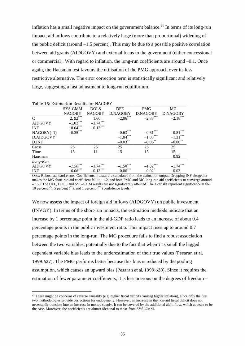
35

inflation has a small negative impact on the government balance.31 In terms of its long-run

impact, aid inflows contribute to a relatively large (more than proportional) widening of

the public deficit (around –1.5 percent). This may be due to a possible positive correlation

between aid grants (AIDGOVY) and external loans to the government (either concessional

or commercial). With regard to inflation, the long-run coefficients are around –0.1. Once

again, the Hausman test favours the utilisation of the PMG approach over its less

restrictive alternative. The error correction term is statistically significant and relatively

large, suggesting a fast adjustment to long-run equilibrium.

Table 15: Estimation Results for NAGOBYSYS-GMM DOLS DFE PMG MGNAGOBY NAGOBY D.NAGOBY D.NAGOBY D.NAGOBY

C 2. 92*** 1.60*** –2.06*** –2.83*** –2.18***

AIDGOVY –1.03*** –1.74***

INF –0.04*** –0.13***

NAGOBY(–1) 0.35*** –0.63*** –0.61*** –0.81***

D.AIDGOVY –1.04*** –1.03*** –1.31***

D.INF –0.03*** –0.06*** –0.06***

Cross 25 25 25 25 25Time 15 11 15 15 15Hausman 0.92***

Long-RunAIDGOVY –1.58*** –1.74*** –1.50*** –1.32*** –1.74***

INF –0.06*** –0.13*** –0.06*** –0.02*** –0.03***

Obs.: Robust standard errors. Coefficients in italic are calculated from the estimation output. Dropping INF altogethermakes the MG short-run aid coefficient fall to –1.2, and both PMG and MG long-run aid coefficients to converge around–1.55. The DFE, DOLS and SYS-GMM results are not significantly affected. The asterisks represent significance at the10 percent (*), 5 percent (**), and 1 percent (***) confidence levels.

We now assess the impact of foreign aid inflows (AIDGOVY) on public investment

(INVGY). In terms of the short-run impacts, the estimation methods indicate that an

increase by 1 percentage point in the aid-GDP ratio leads to an increase of about 0.4

percentage points in the public investment ratio. This impact rises up to around 0.7

percentage points in the long-run. The MG procedure fails to find a robust association

between the two variables, potentially due to the fact that when T is small the lagged

dependent variable bias leads to the underestimation of their true values (Pesaran et al,

1999:627). The PMG performs better because this bias is reduced by the pooling

assumption, which causes an upward bias (Pesaran et al, 1999:628). Since it requires the

estimation of fewer parameter coefficients, it is less onerous on the degrees of freedom –

31 There might be concerns of reverse causality (e.g. higher fiscal deficits causing higher inflation), since only the firsttwo methodologies provide corrections for endogeneity. However, an increase in the non-aid fiscal deficit does notnecessarily translate into an increase in money supply. It can be covered by the additional aid inflow, which appears to bethe case. Moreover, the coefficients are almost identical to those from SYS-GMM.

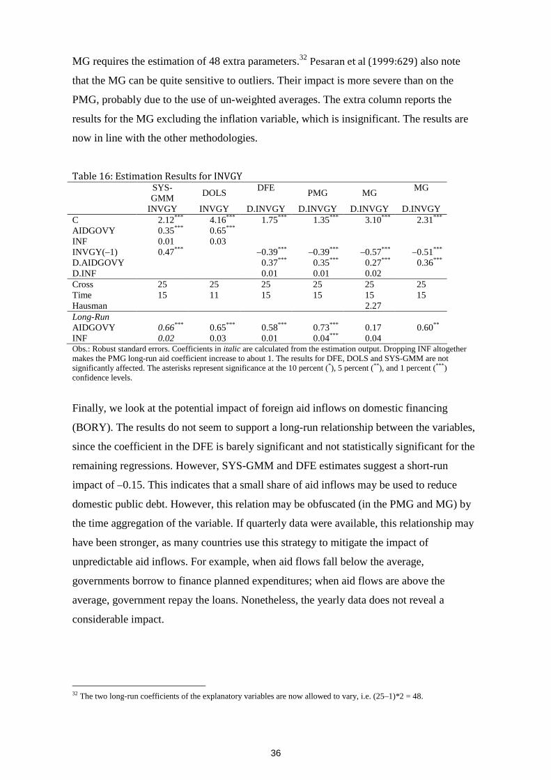
36

MG requires the estimation of 48 extra parameters.32Pesaran et al (1999:629) also note

that the MG can be quite sensitive to outliers. Their impact is more severe than on the

PMG, probably due to the use of un-weighted averages. The extra column reports the

results for the MG excluding the inflation variable, which is insignificant. The results are

now in line with the other methodologies.

Table 16: Estimation Results for INVGYSYS-GMM

DOLSDFE

PMG MGMG

INVGY INVGY D.INVGY D.INVGY D.INVGY D.INVGYC 2.12*** 4.16*** 1.75*** 1.35*** 3.10*** 2.31***

AIDGOVY 0.35*** 0.65***

INF 0.01*** 0.03***

INVGY(–1) 0.47*** –0.39*** –0.39*** –0.57*** –0.51***

D.AIDGOVY 0.37*** 0.35*** 0.27*** 0.36***

D.INF 0.01*** 0.01*** 0.02***

Cross 25 25 25 25 25 25Time 15 11 15 15 15 15Hausman 2.27***

Long-RunAIDGOVY 0.66*** 0.65*** 0.58*** 0.73*** 0.17*** 0.60***

INF 0.02*** 0.03*** 0.01*** 0.04*** 0.04***

Obs.: Robust standard errors. Coefficients in italic are calculated from the estimation output. Dropping INF altogethermakes the PMG long-run aid coefficient increase to about 1. The results for DFE, DOLS and SYS-GMM are notsignificantly affected. The asterisks represent significance at the 10 percent (*), 5 percent (**), and 1 percent (***)confidence levels.

Finally, we look at the potential impact of foreign aid inflows on domestic financing

(BORY). The results do not seem to support a long-run relationship between the variables,

since the coefficient in the DFE is barely significant and not statistically significant for the

remaining regressions. However, SYS-GMM and DFE estimates suggest a short-run

impact of –0.15. This indicates that a small share of aid inflows may be used to reduce

domestic public debt. However, this relation may be obfuscated (in the PMG and MG) by

the time aggregation of the variable. If quarterly data were available, this relationship may

have been stronger, as many countries use this strategy to mitigate the impact of

unpredictable aid inflows. For example, when aid flows fall below the average,

governments borrow to finance planned expenditures; when aid flows are above the

average, government repay the loans. Nonetheless, the yearly data does not reveal a

considerable impact.

32 The two long-run coefficients of the explanatory variables are now allowed to vary, i.e. (25–1)*2 = 48.

37

Table 17: Estimation Results for BORYSYS-GMM

DOLSDFE

PMG MG

BORY BORY D.BORY D.BORY D.BORYC 1.56*** 0.96*** 1.36*** 0.90*** 0.32***

AIDGOVY –0.15*** 0.02***

INF –0.01*** –0.01***

BORY(–1) 0.13*** –0.82*** –0.84*** –0.95***

D.AIDGOVY –0.15*** –0.23*** –0.09***

D.INF –0.01*** 0.03*** 0.04***

Cross 25 25 25 25 25Time 15 11 15 15 15Hausman 0.70***

Long-RunAIDGOVY –0.17*** 0.02*** –0.13*** –0.02*** –0.17***

INF 0.01*** –0.01*** –0.01*** –0.01*** 0.04***

Obs.: Robust standard errors. Coefficients in italic are calculated from the estimation output. Dropping INF altogetherdoes not significantly affect the results (even for DFE). The asterisks represent significance at the 10 percent (*), 5percent (**), and 1 percent (***) confidence levels.

The table below provides a summary of the impacts of foreign aid inflows on the

macroeconomic and fiscal sphere. Starting with absorption, the results suggest that foreign

aid inflows have had significant short- and long-run impact on the non-aid current account

balance (NACABY). The short-run results for the SYS-GMM are significantly lower than

the other empirical methods, possibly due to a downward bias induced by the presence of

the lagged dependent variable. Overall, it seems that around two-thirds of the aid flows are

used to increase the (non-aid) current account deficit, most likely through making foreign

exchange available to domestic importers of goods and services. In the long-run, the

impact of aid is significantly higher for the SYS-GMM, which even suggests full

absorption. The PMG coefficient is lower than that of the DFE and MG, but on the whole

the evidence points to a high level of absorption. With regard to the accumulation of

international reserves (DRY), the fixed-effects models do not reveal a significant short-run

impact, while the heterogeneous alternatives suggest that about one-third of the foreign

exchange provided by aid transfers is kept as central banks’ foreign reserves. In the long-

run, only the PMG appears to indicate a statistically significant effect, albeit lower than the

short-run impact. In light of the PMG and MG results, and bearing in mind the

macroeconomic identity below, there is only weak evidence that aid flows are ‘exiting’

through the capital account (capital outflows), as the sum of the (short-run) impacts on

DRY and NACABY is approximately 1.33

38

The implication is that short-run aid absorption in African countries is higher than

previously suggested by Berg et al (2007) and Aiyar and Ruthbah (2008). Moreover, aid

resources are also found to be used (in the short-run) to build up international reserves,

perhaps to strengthen the capacity to weather external shocks.

Table 18: The Impact of Aid InflowsSYS-GMM

DOLSDFE

PMG MG1

Short-runNACABY –0.43*** n/a*** –0.63*** –0.63*** –0.76***

DRY 0.08*** n/a*** –0.06*** –0.27*** –0. 31***

NAGOBY –1.03*** n/a*** –1.04*** –1.03*** –1.31***

INVGY 0.47*** n/a*** 0.37*** 0.35*** 0.36***

BORY –0.15*** n/a*** –0.15*** –0.23*** –0.09***

Long-RunNACABY –1.13*** –0.86*** –0.76*** –0.62*** –0.96***

DRY 0.00*** 0.13*** 0.01*** –0.11*** –0.11***

NAGOBY –1.58*** –1.74*** –1.50*** –1.32*** –1.74***

INVGY 0.66*** 0.65*** 0.58*** 0.73*** 0.60***

BORY –0.17*** 0.02*** –0.13*** –0.02*** –0.17***

Obs.: 1 The MG results for INVGY exclude inflation. The asterisks represent significance at the 10 percent (*), 5 percent(**), and 1 percent (***) confidence levels.

Turning to spending, the empirical results imply that aid inflows have had large short- and

long-run impacts on the non-aid government balance (NAGOBY). In fact, aid is fully spent

in the short-run. This means that the full amount of aid is used to either (i) boost public

expenditures; (ii) reduce taxes; or (iii) a mixture of both. Full spending is not compatible

with the hypothesis that governments ‘save’ aid resources to pay government debt (either

domestic or foreign). In the long-run, the impact on NAGOBY grows to about 1.5, a more

than proportional impact. This finding is similar to that of Aiyar and Ruthbah (2008). This

may either be a symptom of aid illusion, or the consequence of a positive correlation

between aid grants (AIDGOVY) and foreign loans. With regard to government investment

(INVGY), about a third of aid resources are used to finance public investment programmes

(in the short-run), rising to two-thirds in the long-run. However, the SYS-GMM short-run

coefficient is notably higher. Finally, only the fixed-effects models uncover significant

short-run impacts on domestic borrowing (BORY), even though these are comparatively

smaller than those for other variables. There is little evidence supporting a long-run

relationship between aid and domestic financing. These results can be analysed with the

support of the following fiscal identity (budget constraint),

33 Note that an increase in DRY means a fall in international reserves.

39

where CY stands for public recurrent spending, TY for domestic revenue, and LY for

external lending (including concessional loans). Bearing in mind the caveat of potential

endogeneity (although addressed by GMM and DOLS estimators), we may argue that the

short-run impact on public investment is somewhere between one-third and one-half of the

aid inflow, leaving about two-thirds or one-half for either increasing recurrent expenditures

or lowering domestic revenues (e.g. taxes). In fact, recurrent spending is the most obvious

candidate, since it often includes several development-related activities (e.g. wages of

nurses, textbooks, etc.). In the long-run, the impact of aid on public investment increases to

two-thirds.

Further to these economic observations, the empirical results may also provide some

information about the ‘small sample’ behaviour of the estimators. As the temporal

dimension (T) increases, the downward bias induced by the lagged dependent variable

tends to decline and even OLS-FE may become consistent. However, these performance

gains are likely to be higher/faster for the ECM models. This may explain why, in the

macroeconomic sample, the SYS-GMM short-run coefficients are significantly lower than

in the other approaches.34 However, the SYS-GMM is likely to outperform the ECM

approach in shorter panels (small T), such as the fiscal sample. In fact, the short-run

coefficients are now higher than those for the PMG and MG – with the exception of

NAGOBY, which are similar. Hence, it appears that the downward bias is stronger in the

SYS-GMM estimator in the macroeconomic sample (T=26), whilst the bias is larger for the

ECM-type models in the fiscal sample (T=16). This implies a trade-off between these

different methodologies.

On the whole, our preferred model is the PMG estimator for two main reasons. Firstly, it

appears that its estimates remain robust in the shorter panel, as opposed to those from the

MG. This robustness may be explained by the fact that imposing parameter homogeneity

often causes an upward bias (in absolute terms) in the lagged dependent variable (Pesaran

et al, 1999:628). Hence, the potential downward bias induced by small T may actually be

reduced or even cancelled out. It can be seen that, in general, the absolute magnitude of the

34 We have also estimated OLS-FE and DIF-GMM for the lagged dependent variable model, and the results indicate thatthese estimators tend to underestimate both short- and long-run impacts in relation to SYS-GMM.

40

estimated error correction coefficients follow the sequence MG>PMG>DFE. Moreover,

the MG is also more sensitive to outliers. Secondly, the PMG assumptions are more

appealing in economic terms. We allow heterogeneity in the short-run responses and the

speed of adjustment to equilibrium, while constraining the long-run relationships to be the

same. This is an appealing middle ground between the strong pooling assumptions of the

DFE (and indeed GMM) estimator and the flexibility of the MG estimator.

However, we should bear in mind the weaknesses of the empirical analysis presented here.

The results from our estimation strategies (including the system GMM) may be sensitive to

the presence of cross-sectional error dependence. If T was significantly larger than N

(which unfortunately is not our case) we could model and test the cross-correlation of the

error terms through seemingly unrelated regressions (SUR). Nonetheless, we can test the

assumption of cross-sectional independence with the Breusch-Pagan LM test statistic and

Pesaran’s (2004) CD statistic. The LM test follows a chi-square distribution with N(N–1)/2

degrees of freedom but requires T>N, whilst the Pesaran test is asymptotically normal. For

both tests we use the DFE specification presented above. Although the results from the LM

statistic strongly reject the hypothesis of cross-sectional independence, the CD statistic

provides much weaker evidence of violations. We recall that the LM statistic relies on

large T and small N and thus may not perform well when both dimensions are of similar

magnitudes. In fact, the computations were just about possible for the macroeconomic

sample, where T=26 and N=25. Thus, we may argue that there is only weak evidence that

the assumption of cross-sectional dependence of the error structures is violated by the data,

and thus the empirical estimates are not likely to be significantly biased. Furthermore,

panel estimators that are robust to cross-sectional dependence are only at an embryonic

stage – e.g. see recent literature on ‘common correlated effects’ estimator (Kapetanios et al,

2009).

Table19: Cross-Sectional Independence TestsDFE model NACABY

AIDBOPYLTOT

DRYAIDBOPYLTOT

NAGOBYAIDGOVYINF

INVGYAIDGOVYINF

BORYAIDGOVYINF

Breusch-Pagan LM statistic 395.88*** 366.76*** n/a*** n/a*** n/a***

Pesaran CD statistic 1.83*** 2.24*** 1.69*** –0.89*** –0.26***

Obs.: Tests results generated by the Stata’s ‘xttest2’ and ‘xtcsd’ modules. CD test results based on DOLS regressions donot reject independence, except for the INVGY equation at 10 percent, whilst the LM statistic cannot be computed (evenfor the macroeconomic sample). The asterisks represent significance at the 10 percent (*), 5 percent (**), and 1 percent(***) confidence levels.

41

Finally, the estimates only represent country averages. Policy responses may vary from

country to country, and therefore this analysis does not preclude the use of other

methodologies to unveil country-specific macroeconomic responses.

6. Conclusion

This paper revisits the issue of macroeconomic management of large aid disbursements.

We have constructed a new panel dataset to investigate the level of aid ‘absorption’ and

‘spending’ in Africa’s low-income countries. Our results suggest that, in the short-run,

recipient countries have absorbed about two-thirds of the aid inflow, using them to increase

the non-aid current account deficit. Moreover, around one-third of the foreign exchange

provided by these inflows has been used to build up international reserves, perhaps to

protect economies from future external shocks.35 In the long-run, absorption of foreign

exchange appears to increase further without reaching its maximum (full absorption). In

terms of ‘aid spending’, recipient countries appear to have fully spent the amount of aid,

using it to increase the non-aid government deficit. In particular, a substantial percentage

of these inflows went to finance public investment expenditures. There is only weak

evidence that some aid flows have been ‘saved’, i.e. used to substitute for domestic

borrowing. Overall, these findings suggest that the macroeconomic management of aid

inflows in Africa has been better than often suggested by comparable exercises.

These results challenge some of the conclusions from Aiyar and Ruthbah (2008), namely

that short-run absorption is usually low, with aid exiting through the capital account. This

may be due to the use of an inappropriate measure of aid flows (DAC’s donor reported aid)

or the application of a methodology that neglects the time series properties of the data.

However, we corroborate the result that spending is higher than absorption, which

represents an injection of domestic liquidity in the recipient country.

35 Buffie et al (2004) suggest that a ‘managed float’ is the most attractive approach to manage shocks to aidinflows, therefore arguing that African central banks have been correct to intervene in the foreign exchangemarket.

42

References:Agénor, P. and P. Montiel (1999), Development Macroeconomics (Second Edition),Princeton University Press, Chichester, West Sussex.

Aiyar, S. and U. Ruthbah (2008), ‘Where Did All the Aid Go? An Empirical Analysis ofAbsorption and Spending.’ IMF Working Paper 08/34, Washington, D.C.

Arellano, M. and S. Bond (1991), ‘Some Tests of Specification for Panel Data: MonteCarlo Evidence and an Application to Employment Equations.’ Review of EconomicStudies, 58:277-297.

Asteriou, D. and S. Hall (2007), Applied Econometrics: A Modern Approach (RevisedEdition), Palgrave McMillan, Basingstoke.

Baltagi, B. (2008), Econometric Analysis of Panel Data (Fourth Edition), John Wiley &Sons, Chichester.

Banerjee, A., M. Marcellino and C. Osbat (2005), ‘Testing for PPP: Should We Use PanelMethods?’ Empirical Economics, 30:77–91.

Banerjee, A., M. Marcellino and C. Osbat (2004), ‘Some Cautions on the Use of PanelMethods for Integrated Series of Macroeconomic Data,’ Econometrics Journal, 7:322-340.

Banerjee, A., J. Dolado and R. Mestre (1998), ‘Error-Correction Mechanism Tests forCointegration in a Single-Equation Framework,’ Journal of Time Series Analysis, 19:267–83.

Berg, A., S. Aiyar, M. Hussain, S. Roache, T. Mirzoev and A. Mahone (2007), ‘TheMacroeconomics of Scaling Up Aid: Lessons from Recent Experience,’ IMF OccasionalPaper 253.

Breitung, J. (2000), ‘The Local Power of Some Unit Root Tests for Panel Data.’ in B.Baltagi (ed.), Advances in Econometrics, Vol. 15: Nonstationary Panels, PanelCointegration, and Dynamic Panels, 161–178, Elsevier Science.

Buffie, E., C. Adam, S. O’Connell and C. Pattillo (2004), ‘Exchange Rate Policy and theManagement of Official and Private Capital Flows in Africa.’ IMF Staff Papers, 51,Special Issue, 126-160.

Calvo, G. and C. Reinhart (2002), ‘Fear of Floating.’ Quarterly Journal of Economics,117(2):379-408.

Choi, I. (2001), ‘Unit Root Tests for Panel Data.’ Journal of International Money andFinance, 20(2):249–272.

Engle, R. and C. Granger (1987), “Co-integration and Error-Correction: Representation,Estimation and Testing.” Econometrica, 55, 251-276.

Foster, M. and T. Killick (2006), ‘What Would Doubling Aid do for MacroeconomicManagement in Africa,’ Overseas Development Institute (ODI) Working Paper 264.

43

Greene, W. (2003), Econometric Analysis (Fifth Edition), Prentice Hall, New Jersey.

Gupta, S., R. Powell and Y. Yang (2006), Macroeconomic Challenges of Scaling Up Aidto Africa: A Checklist for Practitioners. International Monetary Fund, Washington, D.C.

Heller, P. (2005), ‘Pity the Finance Minister: Issues in Managing a Substantial Scaling Upof Aid Flows,’ IMF Working Paper 05/180.

Hadri, K. (2000), ‘Testing for Stationarity in Heterogeneous Panel Data.’ EconometricsJournal, 3:148–161.

Hussain, M., A. Berg and S. Aiyar (2009), ‘The Macroeconomic Management of IncreasedAid: Policy Lessons from Recent Experience.’ Review of Development Economics, 13(3),491-509.

Im, K., H. Pesaran and Y. Shin (2003), ‘Testing for Unit Roots in Heterogeneous Panels.’Journal of Econometrics, 115:53–74.

IMF (2005), ‘The Macroeconomics of Managing Increased Aid Inflows: Experiences ofLow-Income Countries and Policy Implications,’ SM/05/306 (August 8, 2005),unpublished, Policy Development and Review Department

Isard, P., L. Lipschitz, A. Mourmouras, and B. Yontcheva, eds. (2006), TheMacroeconomic Management of Foreign Aid: Opportunities and Pitfalls, Washington:International Monetary Fund.

Johansen, S. (1988), “Statistical Analysis of Cointegration Vectors.” Journal of EconomicDynamics and Control, 12(2-3), 231-254

Kao, C. and M. Chiang (2000), ‘On the Estimation and Inference of a CointegratedRegression in Panel Data.’ In B. Baltagi (ed.), Advances in Econometrics, Vol. 15:Nonstationary Panels, Panel Cointegration, and Dynamic Panels, 179-222, ElsevierScience.

Kao, C. (1999), ‘Spurious Regression and Residual-Based Tests for Cointegration in PanelData.’ Journal of Econometrics, 90:1–44.

Kapetanios, G., H. Pesaran and T. Yamagata (2009), ‘Panels with NonstationaryMultifactor Error Structures.’ Cambridge Working Papers in Economics, 0651 (Revised),University of Cambridge.

Larsson, R., J. Lyhagen and M. Lothgren (2001), ’Likelihood-Based Cointegration Tests inHeterogeneous Panels.’ Econometrics Journal, 4:109–142.

Levin, A., C. Lin and C. Chu (2002), ‘Unit Root Tests in Panel Data: Asymptotic andFinite-Sample Properties.’ Journal of Econometrics, 108:1–24.

Maddala, G. and S. Wu (1999). ‘A Comparative Study of Unit Root Tests with Panel Dataand a New Simple Test.’ Oxford Bulletin of Economics and Statistics, 61:631–52.

44

McKinley, T. (2005), “Why is the Dutch Disease Always a Disease? The MacroeconomicConsequences of Scaling Up ODA.” UNDP, International Poverty Centre, Working Paper10.

Pedroni, P. (2004), ‘Panel Cointegration; Asymptotic and Finite Sample Properties ofPooled Time Series Tests with an Application to the PPP Hypothesis.’ EconometricTheory, 20, 597-625.

Pedroni, P. (2000), ‘Fully Modified OLS for Heterogeneous Cointegrated Panels.’ In B.Baltagi (ed.), Advances in Econometrics, Vol. 15: Nonstationary Panels, PanelCointegration, and Dynamic Panels, 93-130, Elsevier Science.

Pedroni, P. (1999), ‘Critical Values for Cointegration Tests in Heterogeneous Panels withMultiple Regressors.’ Oxford Bulletin of Economics and Statistics, 61:653–70.

Pesaran, H. (2007), ‘A Simple Panel Unit Root Test in the Presence of Cross-SectionDependence.’ Journal of Applied Econometrics, 22(2), 265-312.

Pesaran, H. (2004), ‘General Diagnostic Tests for Cross Section Dependence in Panels.’Cambridge Working Papers in Economics 0435, Faculty of Economics, University ofCambridge.

Pesaran, H., Y. Shin and R. Smith (1999), ‘Pooled Mean Group Estimation of DynamicHeterogeneous Panels.’ Journal of the American Statistical Association, 94(446):621–634.

Phillips, P. and H. Moon (1999), ‘Linear Regression Limit Theory for Nonstationary PanelData.’ Econometrica, 67(5):1057-1111.

Phillips, P. and B. Hansen (1990), ‘Statistical Inference in Instrumental Variables Regressionwith I(1) Processes.’ The Review of Economic Studies, 57(1), 99-125.

Prati, A., R. Sahay and T. Tressel (2003), ‘Is There a Case for Sterilizing Foreign Aid Inflows?’Paper presented at the Research Workshop ‘Macroeconomic Challenges in Low IncomeCountries’, October 23-24, Washington D.C.: IMF.

QMS (2007), EViews 6 User’s Guide II, Quantitative Micro Software, LLC.

Roodman, D. (2009), ‘A Note on the Theme of Too Many Instruments.’ Oxford Bulletin ofEconomics and Statistics, 71(1), 135–158.

Saikkonen, P. (1991), ‘Asymptotically Efficient Estimation of Cointegration Regressions.’Econometric Theory, 7(1), 1-21.

Stock, J. and M. Watson (1993), ‘A Simple Estimator of Cointegrating Vectors in HigherOrder Integrated Systems.’ Econometrica, 61(4), 783-820.

Westerlund, J. (2007), ‘Testing for Error Correction in Panel Data.’ Oxford Bulletin ofEconomics and Statistics, 69(6), 709-748.

45

White, H. (2005), ‘The Case for Doubling Aid.’ IDS Bulletin, 36(3), 8-13.

White, H. (1992), ‘The Macroeconomic Impact of Development Aid: A Critical Survey.’Journal of Development Studies, 28(2), 163-240.

46

Appendix

In this Appendix, we compare our data with the country-specific estimates reported in IMF

(2005) and Hussain et al (2009). For that purpose, we estimate country-level regressions for

the following five African countries: Ethiopia, Ghana, Mozambique, Tanzania and Uganda.

Since the samples for absorption and spending only include 26 and 16 time observations,

respectively, these results should be interpreted with great caution. These estimates are far

less robust than our panel analysis (especially individual DOLS), and should only be taken as

indicative. Moreover, the heterogeneous short-run effects from the PMG estimator are also

reported.

Table 20: Country-Specific Results (Impact of Aid)Absorption (NACABY) Spending (NAGOBY)PMG ECM DOLS PMG ECM DOLS

IMFSR SR LR LR

IMFSR SR LR LR

Ethiopia ID19 -0.20 -0.47 -0.73 -2.50 -0.73 0.14 -0.55 -0.32 -0.68 3.76Ghana ID22 1.82 -0.03 0.12 -0.25 2.06 -0.07 -0.70 -0.31 -0.38 0.21Mozambique ID35 -0.66 -1.38 -1.33 -1.60 -1.53 -1.08 -1.51 -1.77 -2.60 -4.70Tanzania ID48 1.05 -1.55 -1.82 -4.76 -3.57 -0.92 -1.76 -4.26 -2.71 -4.97Uganda ID51 -0.28 -0.79 -1.22 -1.77 -1.44 -0.75 -1.53 -1.79 -1.86 -2.22Obs.: The IMF values are recalculated and estimates in italic indicate that the original publication truncated them (i.e.bound them to the interval -1 to 0). The estimates in bold are statistically significant. DOLS regressions include only 1lead and 1 lag to reduce estimated parameters.

The results appear to suggest that absorption and spending are quite high for Mozambique,

Tanzania and Uganda. In fact, most estimates point to (more than) full absorption and

spending in both the short- and long-run. The estimates for Ethiopia and Ghana exhibit

higher standard errors, hence we are not able to accept them as statistically significant.

Nonetheless, most of their values are higher than the IMF estimates. The table below

reports the same results, in a more tractable format.

Table 21: Absorption and SpendingAbsorption (%) Spending (%)

PMG ECM DOLS PMG ECM DOLSIMF

SR SR LR LRIMF

SR SR LR LREthiopia ID19 20% 47% 73% 100% 73% 0% 55% 32% 68% 0%Ghana ID22 0% 3% 0% 25% 0% 7% 70% 31% 38% 0%Mozambique ID35 66% 100% 100% 100% 100% 100% 100% 100% 100% 100%Tanzania ID48 0% 100% 100% 100% 100% 92% 100% 100% 100% 100%Uganda ID51 28% 79% 100% 100% 100% 75% 100% 100% 100% 100%Obs.: Values are truncated.