LECTURE 8Monetary Policy at the Zero Lower Bound

October 19, 2011

Economics 210c/236a Christina RomerFall 2011 David Romer

I. PAUL KRUGMAN, “IT’S BAAACK: JAPAN’S SLUMP AND

THE RETURN OF THE LIQUIDITY TRAP”

Krugman’s Baseline Model – Assumptions (I)

• Discrete time.

• Identical, infinitely-lived agents.

• Representative agent has U = ∑tDt ln ct, 0 < D < 1.

• Each agent receives an endowment y of the consumption good each period.

• Can sell endowment for money, and buy goods with money.

• Economy is competitive and prices are perfectly flexible (!).

• Perfect foresight.

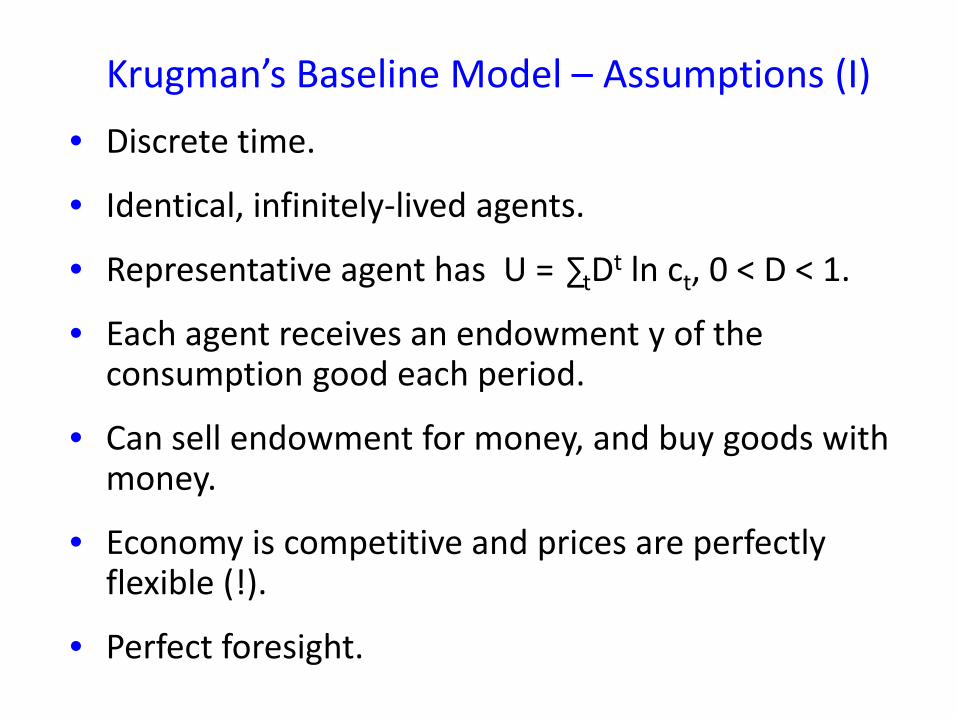
Krugman’s Baseline Model – Assumptions (II)

• Cash-in-advance constraint. Within period t:

• Agents start with some holdings of money and bonds (from period t-1).

• There’s then a market for trading money and bonds.

• Call the representative agent’s holdings after these trades Mt and Bt.

• The cash-in-advance constraint is ct ≤ Mt/Pt.

• After the agent has bought and sold goods, it receives interest on its bond holdings, and any lump-sum taxes or transfers are implemented.

• The cash-in-advance constraint and perfect foresight imply that ct = Mt/Pt or it = 0 (or both).

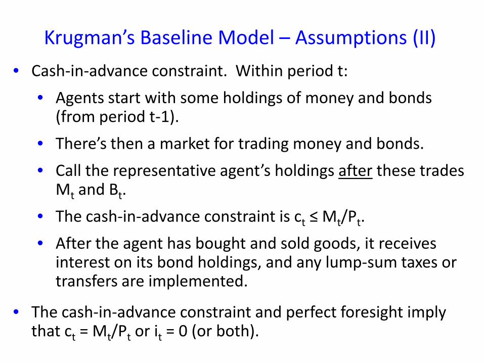
Households’ First-Order Condition

• Suppose the economy is in equilibrium, and consider an agent thinking of spending $1 less on ct and using the proceeds to increase ct+1.

•

•

• => … => (*)

• Note that this holds even if it = 0.

)y/1)(P/1(MC t=

)y/D](P/)i1[(MB 1tt ++=

1)P/P)(D/1(i t1tt −= +

The Steady State with Constant M

• Suppose M is constant at some level (denoted M*).

• If there is a steady state, P is constant. Call this P*.

• Then equation (*), , simplifies to for all t, or

• Note that i* > 0.

1)P/P)(D/1(i t1tt −= +

1)D/1(it −= .D/)D1(*i −=

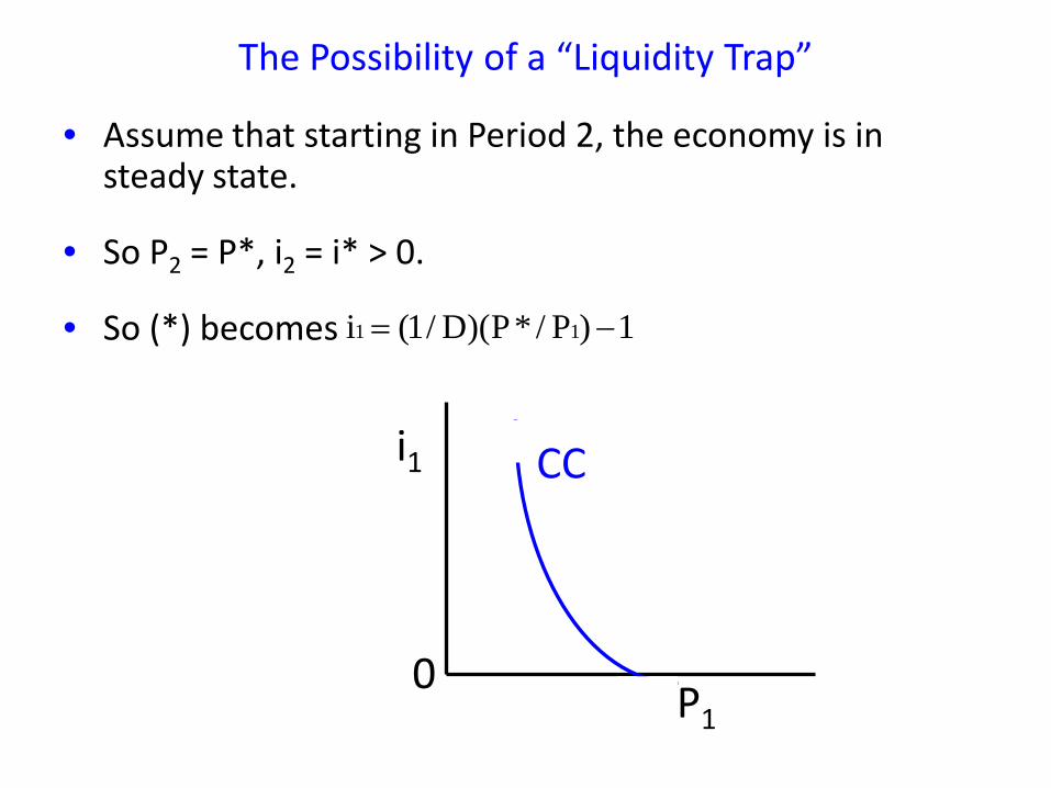
The Possibility of a “Liquidity Trap”

• Assume that starting in Period 2, the economy is in steady state.

• So P2 = P*, i2 = i* > 0.

• So (*) becomes 1)P/*P)(D/1(i 11 −=

0

i1

P1

CC

The Possibility of a “Liquidity Trap” (cont.)

• Households’ allocation of wealth between money and bonds in period 1:

• If i1 > 0: M1/P1 = y => P1 = M1/y.

• If i1 = 0: M1/P1 ≥ y => P1 ≤ M1/y.

0

i1

P1

MM

The Effects of an Increase in M1 when i1 > 0

i1

0P1

CCMM

MM’

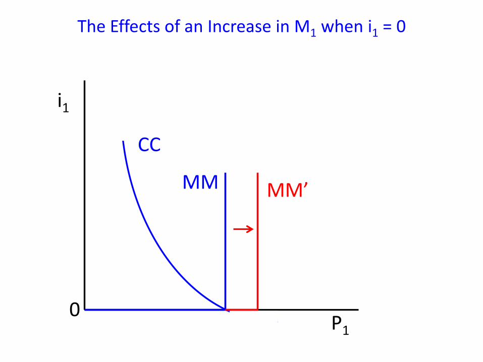
The Effects of an Increase in M1 when i1 = 0

i1

0P1

CC

MM MM’

The Effects of an Increase in M* when i1 = 0

i1

0P1

CC

MM

Recall CC equation: i1 = (1/D)(P*/P1) - 1

CC’

Some More Experiments (I)

• Suppose the economy is in a liquidity trap in periods 1 and 2, then in steady state with i = i* > 0. Raising M1 or M2 has no effect on aggregate demand in any period. But raising M* raises aggregate demand in period 2 and in period 1.

• Continue to assume a liquidity trap in period 1 and steady state starting in period 3. Suppose initially i2 > 0. Raising M2to the point where i2 = 0 raises aggregate demand in period 1. That is, when the economy is in a liquidity trap, promising to stay in the trap longer rises aggregate demand.

Some More Experiments (II)

• Consider raising M by the same proportion in all periods. Then P rises by the same proportion in all periods.

• Suppose the economy is in steady state starting in period 2, and suppose the central bank targets a zero inflation rate from period 1 to period 2. Thus its choice of M* moves one-for-one with movements in P1. Then if something pushes the equilibrium real rate in period 1 below 0, there is no equilibrium: P1 falls without limit. Inflation targeting eliminates any nominal anchor for the economy.

FOMC Statement, Aug. 12, 2003

“The Committee judges that, on balance, the risk of inflation becoming undesirably low is likely to be the predominant concern for the foreseeable future. In these circumstances, the Committee believes that policy accommodation can be maintained for a considerable period.”

II. BEN BERNANKE, “JAPANESE MONETARY POLICY: A CASE OF SELF-INDUCED PARALYSIS?”

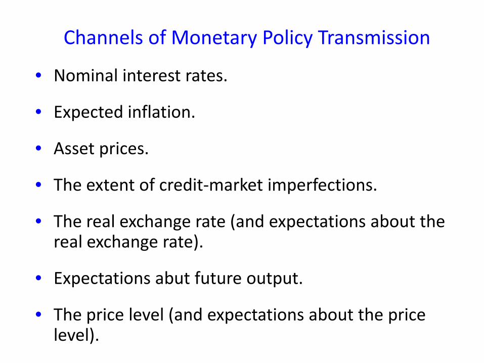
Channels of Monetary Policy Transmission

• Nominal interest rates.

• Expected inflation.

• Asset prices.

• The extent of credit-market imperfections.

• The real exchange rate (and expectations about the real exchange rate).

• Expectations abut future output.

• The price level (and expectations about the price level).

Tools of Monetary Policy at the Zero Lower Bound

• Communication about objectives, or the formal adoption of new objectives.

• Communication about future path of safe short-term interest rate (or of supply of high-powered money).

• Communication about the channels of monetary policy (such as the exchange rate or future output).

• Purchases of assets other than short-term government debt.

• Conventional open-market operations?

• Money-financed fiscal expansions (helicopter drops)?

Some Important Questions

• Could some of the tools be counterproductive?

• Could the mix of outcomes (especially, in terms of output and inflation) be different for these tools than for conventional open-market operations in normal times?

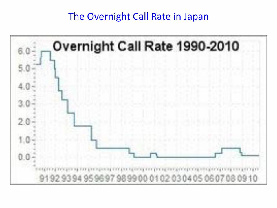
The Overnight Call Rate in Japan

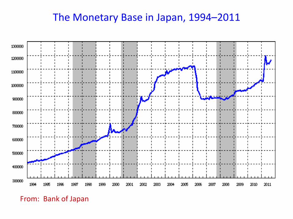
The Monetary Base in Japan, 1994–2011

From: Bank of Japan

III. OVERVIEW

0

1

2

3

4

5

6

Jan-

29

Jul-2

9

Jan-

30

Jul-3

0

Jan-

31

Jul-3

1

Jan-

32

Jul-3

2

Jan-

33

Jul-3

3

Jan-

34

Jul-3

4

Jan-

35

Jul-3

5

Nominal Interest Rate on 3- to 6-month Treasury Notes

IV. GAUTI EGGERTSSON, “GREAT EXPECTATIONS AND THE

END OF THE DEPRESSION”

1929

-01

1929

-05

1929

-09

1930

-01

1930

-05

1930

-09

1931

-01

1931

-05

1931

-09

1932

-01

1932

-05

1932

-09

1933

-01

1933

-05

1933

-09

1934

-01

1934

-05

1934

-09

1935

-01

1935

-05

1935

-09

1936

-01

1936

-05

1936

-09

1937

-01

1937

-05

1937

-09

1

1.2

1.4

1.6

1.8

2

2.2

2.4

Indu

stri

al P

rodu

ctio

n (L

ogar

ithm

s)Industrial Production

2.3

2.4

2.5

2.6

2.7

2.8

2.9Ja

n-29

Jun-

29

Nov

-29

Apr

-30

Sep-

30

Feb-

31

Jul-3

1

Dec

-31

May

-32

Oct

-32

Mar

-33

Aug

-33

Jan-

34

Jun-

34

Nov

-34

Apr

-35

Sep-

35

Feb-

36

Jul-3

6

Dec

-36

May

-37

Oct

-37

Prod

ucer

Pri

ce In

dex,

Log

arith

ms

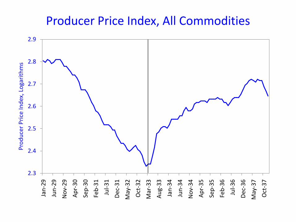
Producer Price Index, All Commodities

2.8

2.9

3

3.1

3.2

3.3

3.4

3.519

32:0

119

32:0

319

32:0

519

32:0

719

32:0

919

32:1

119

33:0

119

33:0

319

33:0

519

33:0

719

33:0

919

33:1

119

34:0

119

34:0

319

34:0

519

34:0

719

34:0

919

34:1

119

35:0

119

35:0

319

35:0

519

35:0

719

35:0

919

35:1

119

36:0

119

36:0

319

36:0

519

36:0

719

36:0

919

36:1

1

Loga

rith

ms

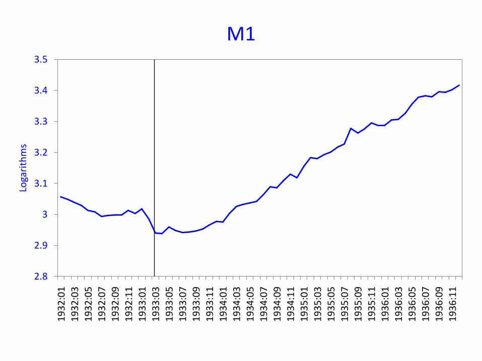
M1

What are the key elements of the regime?

• Gold standard

• Commitment to a balanced budget

• Belief in small government

What is the mechanism by which the regime change affected inflationary expectations?

• Fiscal expansion gives the government an incentive to inflate.

• So, fiscal expansion leads to monetary expansion.

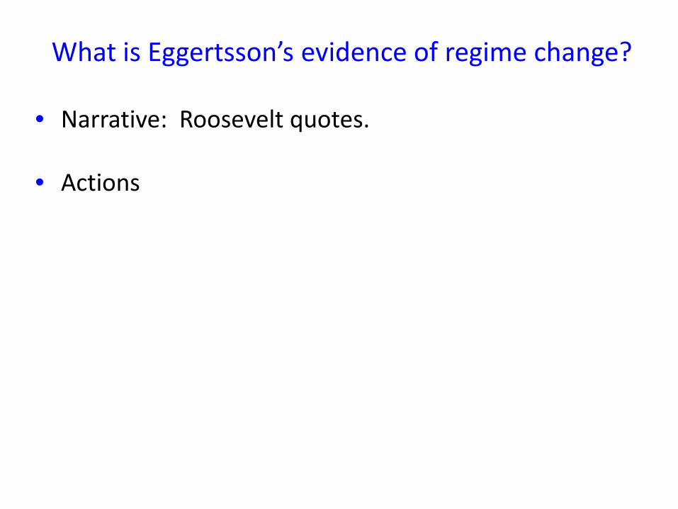
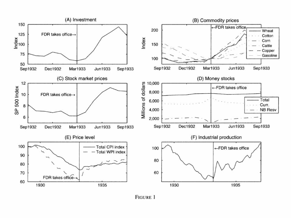
What is Eggertsson’s evidence of regime change?

• Narrative: Roosevelt quotes.

• Actions

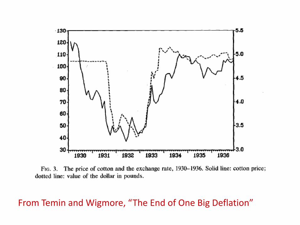
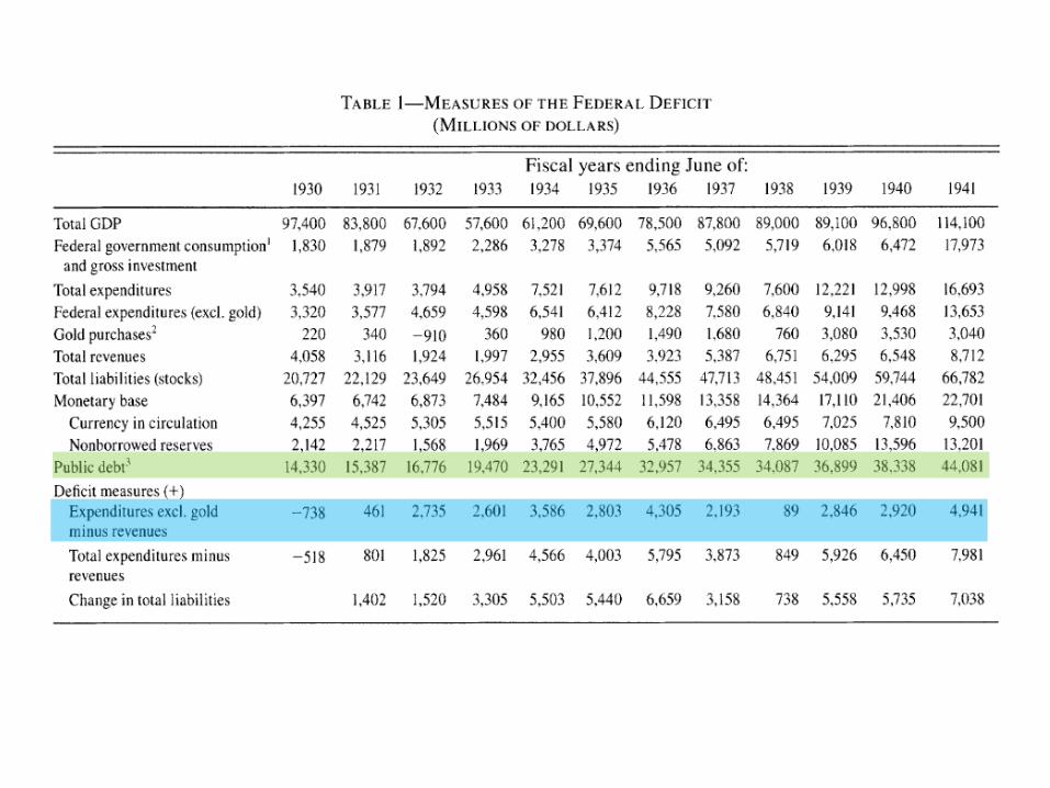
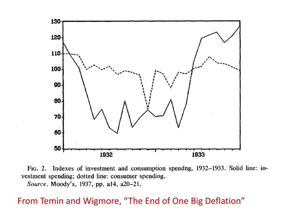
From Temin and Wigmore, “The End of One Big Deflation”

Evaluation of Evidence

• Timing of actions

• What happened to spending?

-10,000

-5,000

0

5,000

10,000

15,000

1930 1931 1932 1933 1934 1935 1936 1937 1938 1939 1940 1941

Federal Receipts, Outlays, and Surplus

Outlays

Receipts

Surplus

From Temin and Wigmore, “The End of One Big Deflation”

From: Temin and Wigmore, “The End of One Big Deflation”

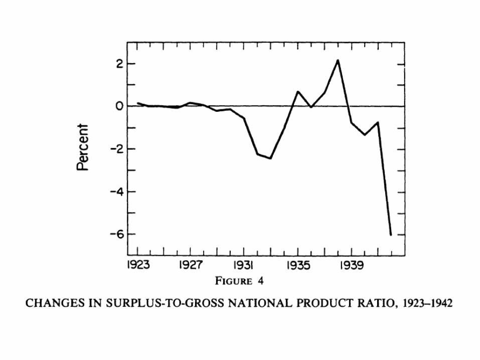
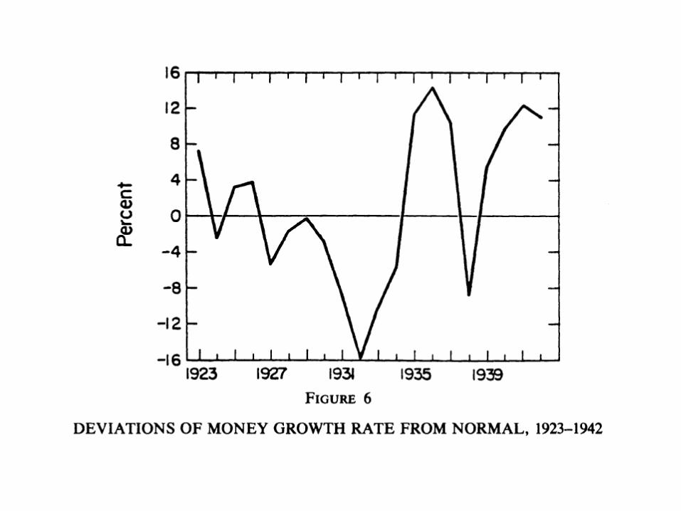
V. CHRISTINA ROMER, “WHAT ENDED THE GREAT

DEPRESSION?”

-500

0

500

1000

1500

2000

2500

3000

3500

4000

4500

1919

1920

1921

1922

1923

1924

1925

1926

1927

1928

1929

1930

1931

1932

1933

1934

1935

1936

1937

1938

1939

1940

Mill

ions

of D

olla

rsGold Inflows to the U.S.

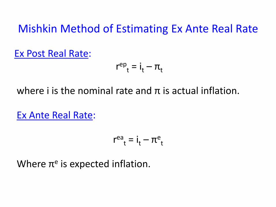
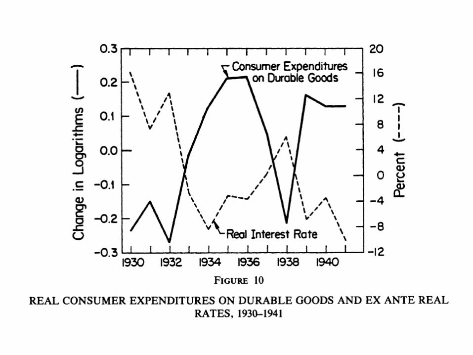
Mishkin Method of Estimating Ex Ante Real Rate

Ex Post Real Rate:rep

t = it – πt

where i is the nominal rate and π is actual inflation.

Ex Ante Real Rate:

reat = it – πe

t

Where πe is expected inflation.

The difference between rep and rea isunanticipated inflation (εt ):

rept = (it – πt)+ (πe

t – πet )

rept = (it – πe

t) – (πt – πet)

= reat – εt

• Under rational expectations, expectation of unanticipated inflation at a point in time is zero.

• You can’t expect to be surprised.

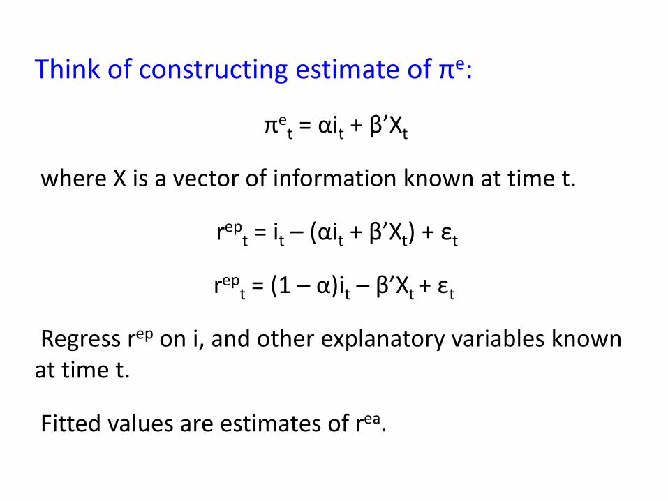
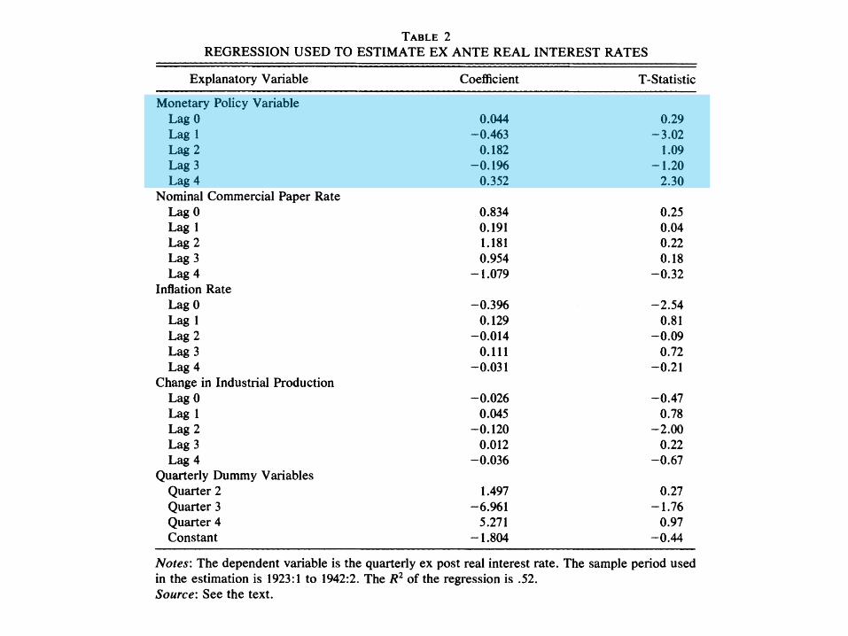
Think of constructing estimate of πe:

πet = αit + β’Xt

where X is a vector of information known at time t.

rept = it – (αit + β’Xt) + εt

rept = (1 – α)it – β’Xt + εt

Regress rep on i, and other explanatory variables known at time t.

Fitted values are estimates of rea.

0

0.5

1

1.5

2

2.5

3

3.5

1929 1930 1931 1932 1933 1934 1935 1936 1937 1938 1939 1940 1941 1942

Behavior of Different Types of Consumer Spending

Nondurables

Services

Durables