Economics 103 Statistics for Economists -...
592
Economics 103 – Statistics for Economists Francis J. DiTraglia University of Pennsylvania
Transcript of Economics 103 Statistics for Economists -...

Economics 103 – Statistics for Economists
Francis J. DiTraglia
University of Pennsylvania

Lecture #1 – Introduction
Overview – Population vs. Sample, Probability vs. Statistics
Polling – Sampling vs. Non-sampling Error, Random Sampling
Causality – Observational vs. Experimental Data, RCTs
Econ 103 Lecture 1 – Slide 1

Racial Discrimination in the Labor MarketSource: Bureau of Labor Statistics
Oct. 2017 Nov. 2017 Dec. 2017
White: 3.2 3.2 3.4
Black/African American: 7.4 7.3 6.6
Table: Unemployment rate in percentage points for men aged 20 and
over in the last quarter of 2017.
The unemployment rate for African Americans has historically been
much higher than for whites. What can this information by itself
tell us about racial discrimination in the labor market?
Econ 103 Lecture 1 – Slide 2

This Course: Use Sample to Learn About Population
Population
Complete set of all items that interest investigator
Sample
Observed subset, or portion, of a population
Sample Size
# of items in the sample, typically denoted n
Examples...
Econ 103 Lecture 1 – Slide 3

In Particular: Use Statistic to Learn about Parameter
Parameter
Numerical measure that describes specific characteristic of a
population.
Statistic
Numerical measure that describes specific characteristic of sample.
Examples...
Econ 103 Lecture 1 – Slide 4

Essential Distinction You Must Remember!
Population
NumericalSummary
Parameter
Sample
NumericalSummary
Statistic
Econ 103 Lecture 1 – Slide 5

This Course
1. Descriptive Statistics: summarize data
I Summary Statistics
I Graphics
2. Probability: Population → Sample
I deductive: “safe” argument
I All ravens are black. Mordecai is a raven, so Mordecai is black.
3. Inferential Statistics: Sample → Population
I inductive: “risky” argument
I I’ve only every seen black ravens, so all ravens must be black.
Econ 103 Lecture 1 – Slide 6

Sampling and Nonsampling Error
In statistics we use samples to learn about populations, but samples
almost never be exactly like the population they are drawn from.
1. Sampling Error
I Random differences between sample and population
I Cancel out on average
I Decreases as sample size grows
2. Nonsampling Error
I Systematic differences between sample and population
I Does not cancel out on average
I Does not decrease as sample size grows
Econ 103 Lecture 1 – Slide 7

Econ 103 Lecture 1 – Slide 8
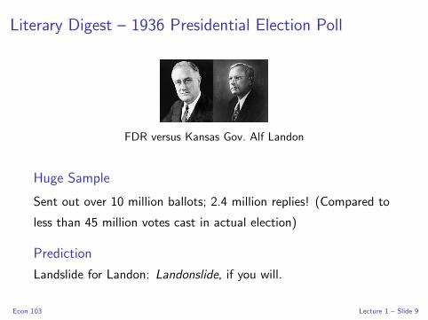
Literary Digest – 1936 Presidential Election Poll
FDR versus Kansas Gov. Alf Landon
Huge Sample
Sent out over 10 million ballots; 2.4 million replies! (Compared to
less than 45 million votes cast in actual election)
Prediction
Landslide for Landon: Landonslide, if you will.
Econ 103 Lecture 1 – Slide 9

Spectacularly Mistaken!
FDR versus Kansas Gov. Alf Landon
Roosevelt Landon
Literary Digest Prediction: 41% 57%
Actual Result: 61% 37%
Econ 103 Lecture 1 – Slide 10

What Went Wrong? Non-sampling Error (aka Bias)
Source: Squire (1988)
Biased Sample
Some units more likely to be sampled than others.
I Ballots mailed those on auto reg. list and in phone books.
Non-response Bias
Even if sample is unbiased, can’t force people to reply.
I Among those who recieved a ballot, Landon supporters were
more likely to reply.
In this case, neither effect alone was enough to throw off the result
but together they did.
Econ 103 Lecture 1 – Slide 11

Randomize to Get an Unbiased Sample
Simple Random Sample
Each member of population is chosen strictly by chance, so that:
(1) selection of one individual doesn’t influence selection of any
other, (2) each individual is just as likely to be chosen, (3) every
possible sample of size n has the same chance of selection.
What about non-response bias? – we’ll come back to this. . .
Econ 103 Lecture 1 – Slide 12

“Negative Views of Trump’s Transition”Source: Pew Research Center
Ahead of Donald Trump’s scheduled press conference in
New York City on Wednesday, the public continues to
give the president-elect low marks for how he is handling
the transition process. . . The latest national survey by
Pew Research Center, conducted Jan. 4-9 among 1,502
adults, finds that 39% approve of the job President-elect
Trump has done so far explaining his policies and plans
for the future to the American people, while a larger
share (55%) say they disapprove.
Econ 103 Lecture 1 – Slide 13

Quantifying Sampling Error95% Confidence Interval for Poll Based on Random Sample
Margin of Error a.k.a. ME
We report P ±ME where ME ≈ 2√P(1− P)/n
Trump Transition Approval Rate
P = 0.39 and n = 1502 so ME ≈ 0.013. We’d report 39% plus or
minus 1.3% if the poll were based on a simple random sample. . .
But Pew Reports an ME of 2.9% – more than twice as large as the
one we calculated! What’s going on here?!
Econ 103 Lecture 1 – Slide 14

Non-response bias is a huge problem. . .Source: Pew Research Center
Econ 103 Lecture 1 – Slide 15

Methodology – “Negative Views of Trump’s Transition”Source: Pew Research Center
The combined landline and cell phone sample are weighted using an
iterative technique that matches gender, age, education, race,
Hispanic origin and nativity and region to parameters from the 2015
Census Bureaus American Community Survey and population
density to parameters from the Decennial Census. The sample also
is weighted to match current patterns of telephone status (landline
only, cell phone only, or both landline and cell phone), based on
extrapolations from the 2016 National Health Interview Survey. The
weighting procedure also accounts for the fact that respondents
with both landline and cell phones have a greater probability of
being included in the combined sample and adjusts for household
size among respondents with a landline phone. The margins of error
reported and statistical tests of significance are adjusted to account
for the surveys design effect, a measure of how much efficiency is
lost from the weighting procedures.Econ 103 Lecture 1 – Slide 16

Simple Example of Weighting a Survey
Post-stratification
I Women make up 49.6% of the population but suppose they are less likely
to respond to your survey than men.
I If women have different opinions of Trump, this will skew the survey.
I Calculate Trump approval rate separately for men PM vs. women PW .
I Report 0.496× PW + 0.504× PM , not the raw approval rate P.
Caveats
I Post-stratification isn’t a magic bullet: you have to figure out what
factors could skew your poll to adjust for them.
I Calculating the ME is more complicated. Since this is an intro class we’ll
focus on simple random samples.
Econ 103 Lecture 1 – Slide 17

Survey to find effect of Polio Vaccine
Ask random sample of parents if they vaccinated their kids or not
and if the kids later developed polio. Compare those who were
vaccinated to those who weren’t.
Would this procedure:
(a) Overstate effectiveness of vaccine
(b) Correctly identify effectiveness of vaccine
(c) Understate effectiveness of vaccine
Econ 103 Lecture 1 – Slide 18

Confounding
Parents who vaccinate their kids may differ systematically from
those who don’t in other ways that impact child’s chance of
contracting polio!
Wealth is related to vaccination and whether child grows up in
a hygenic environment.
Confounder
Factor that influences both outcomes and whether subjects are
treated or not. Masks true effect of treatment.
Econ 103 Lecture 1 – Slide 19

Experiment Using Random Assignment: Randomized
Experiment
Treatment Group Gets Vaccine, Control Group Doesn’t
Essential Point!
Random assignment neutralizes effect of all confounding factors:
since groups are initially equal, on average, any difference that
emerges must be the treatment effect.
Placebo Effect and Randomized Double Blind Experiment
Econ 103 Lecture 1 – Slide 20

Pool ofExperimentalSubjects
Randomly dividedinto two groups
Subjects Blind
Experimenters Blind
Control
Evaluation
Treatment
Evaluation
Econ 103 Lecture 1 – Slide 21

Gold Standard: Randomized, Double-blind Experiment
Randomized blind experiments ensure that on average
the two groups are initially equal, and continue to be
treated equally. Thus a fair comparison is possible.
Randomized, double-blind experiments are considered the
“gold standard” for untangling causation.
Sugar Doesn’t Make Kids Hyper
http://www.youtube.com/watch?v=mkr9YsmrPAI
Econ 103 Lecture 1 – Slide 22

Randomization is not always possible, practical, or ethical.
Observational Data
Data that do not come from a randomized experiment.
It much more challenging to untangle cause and effect using
observational data because of confounders. But sometimes it’s
all we have.
Econ 103 Lecture 1 – Slide 23

Racial Bias in the Labor Market
Bertrand & Mullainathan (2004, American Economic Review)
When faced with observably similar African-American and White
applicants, do they [employers] favor the White one? Some argue
yes, citing either employer prejudice or employer perception that
race signals lower productivity. Others argue that differential
treatment by race is a relic of the past . . . Data limitations make it
difficult to empirically test these views. Since researchers possess far
less data than employers do, White and African-American workers
that appear similar to researchers may look very different to
employers. So any racial difference in labor market outcomes could
just as easily be attributed to differences that are observable to
employers but unobservable to researchers.
Econ 103 Lecture 1 – Slide 24

Racial Bias in the Labor Market: continued . . .
Bertrand & Mullainathan (2004, American Economic Review)
To circumvent this difficulty, we conduct a field experiment . . .We
send resumes in response to help-wanted ads in Chicago and Boston
newspapers and measure call-back for interview for each sent
resume. We experimentally manipulate the perception of race via
the name of the ficticious job applicant. We randomly assign very
White-sounding names (such as Emily Walsh or Greg Baker) to half
the resumes and very African-American-soundsing names (such as
Lakisha Washington or Jamal Jones) to the other half.
Econ 103 Lecture 1 – Slide 25

Racial Bias in the Labor Market: continued . . .
Bertrand & Mullainathan (2004, American Economic Review)
Sample White Names African-American Names
All sent resumes 9.7 6.5
Females 9.9 6.6
Males 8.9 5.8
Table: % Callback by racial soundingness of names.
Later this semester: if there were no racial bias in callbacks, what
is the chance that we would observe such large differences?
Econ 103 Lecture 1 – Slide 26

Lecture #2 – Summary Statistics Part I
Class Survey
Types of Variables
Frequency, Relative Frequency, & Histograms
Measures of Central Tendency
Measures of Variability / Spread
Econ 103 Lecture 2 – Slide 1

Class Survey
I Collect some data to analyze later in the semester.
I None of the questions are sensitive and your name will not be
linked to your responses. I will post an anonymized version of
the dataset on my website.
I The survey is strictly voluntary – if you don’t want to
participate, you don’t have to.
Econ 103 Lecture 2 – Slide 2

Multiple Choice Entry – What is your biological sex?
(a) Male
(b) Female
Econ 103 Lecture 2 – Slide 3

Numeric Entry – How Many Credits?
How many credits are you taking this semester? Please respond
using your remote.
Econ 103 Lecture 2 – Slide 4

Multiple Choice – Class Standing
What is your class standing at Penn?
(a) Freshman
(b) Sophomore
(c) Junior
(d) Senior
Econ 103 Lecture 2 – Slide 5

Multiple Choice – What is Your Eye Color?
Please enter your eye color using your remote.
(a) Black
(b) Blue
(c) Brown
(d) Green
(e) Gray
(f) Green
(g) Hazel
(h) Other
Econ 103 Lecture 2 – Slide 6

How Right-Handed are You?
The sheet in front of you contains a handedness inventory. Please
complete it and calculate your handedness score:
Right− Left
Right + Left
When finished, enter your score using your remote.
Econ 103 Lecture 2 – Slide 7

What is your Height in Inches?
Using your remote, please enter your height in inches, rounded to
the nearest inch:
4ft = 48in
5ft = 60in
6ft = 72in
7ft = 84in
Econ 103 Lecture 2 – Slide 8

What is your Hand Span (in cm)?
On the sheet in front of you is a ruler. Please use it to measure the
span of your right hand in centimeters, to the nearest 1/2 cm.
Hand Span: the distance from thumb to little finger
when your fingers are spread apart
When ready, enter your measurement using your remote.
Econ 103 Lecture 2 – Slide 9
We chose (by computer) a random number between 0 and 100.
The number selected and assigned to you is written on the slip of
paper in front of you. Please do not show your number to anyone
else or look at anyone else’s number.
Please enter your number now using your remote.
Econ 103 Lecture 2 – Slide 10

Call your random number X. Do you think that the percentage of
countries, among all those in the United Nations, that are in Africa
is higher or lower than X?
(a) Higher
(b) Lower
Please answer using your remote.
Econ 103 Lecture 2 – Slide 11

What is your best estimate of the percentage of countries, among
all those that are in the United Nations, that are in Africa?
Please enter your answer using your remote.
Econ 103 Lecture 2 – Slide 12

Types of Variables
Categorical
Qualitative, assigns each unit to category, number either
meaningless or indicates order only
Nominal no order to the categories
Ordinal categories with natural order
Numerical
Quantitative, number meaningful
Discrete Value from discrete set (often count data)
Continuous Value could conceptually be any real number within
some range (though measurements have finite
precision)
Econ 103 Lecture 2 – Slide 13

Types of Variables – Examples
Categorical (called Factor in R)
Nominal eye color, sex
Ordinal course evaluations (0 = Poor, 1 = Fair, . . . )
Numerical
Discrete credits you are taking this semester
Continuous height, handspan, handedness (from survey)
Econ 103 Lecture 2 – Slide 14
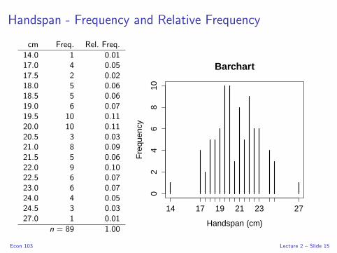
Handspan - Frequency and Relative Frequency
cm Freq. Rel. Freq.
14.0 1 0.0117.0 4 0.0517.5 2 0.0218.0 5 0.0618.5 5 0.0619.0 6 0.0719.5 10 0.1120.0 10 0.1120.5 3 0.0321.0 8 0.0921.5 5 0.0622.0 9 0.1022.5 6 0.0723.0 6 0.0724.0 4 0.0524.5 3 0.0327.0 1 0.01
n = 89 1.00
02
46
810
Barchart
Handspan (cm)
Fre
quen
cy
14 17 19 21 23 27
Econ 103 Lecture 2 – Slide 15

Handspan - Summarize Barchart by “Smoothing”
cm Freq. Rel. Freq.
14.0 1 0.0117.0 4 0.0517.5 2 0.0218.0 5 0.0618.5 5 0.0619.0 6 0.0719.5 10 0.1120.0 10 0.1120.5 3 0.0321.0 8 0.0921.5 5 0.0622.0 9 0.1022.5 6 0.0723.0 6 0.0724.0 4 0.0524.5 3 0.0327.0 1 0.01
n = 88 1.00
Group data into non-overlapping bins of equalwidth:
Bins Freq. Rel. Freq.
[14, 16) 1 0.01[16, 18) 6 0.07[18, 20) 26 0.30[20, 22) 26 0.30[22, 24) 21 0.24[24, 26) 7 0.08[26, 28) 1 0.01
n = 88 1.00
Econ 103 Lecture 2 – Slide 16

Histogram – Density Estimate by Smoothing Barchart
Bins Freq. Rel. Freq.
[14, 16) 1 0.01[16, 18) 6 0.07[18, 20) 26 0.30[20, 22) 26 0.30[22, 24) 21 0.24[24, 26) 7 0.08[26, 28) 1 0.01
n = 88 1.00
14 16 18 20 22 24 26 28
0.00
0.05
0.10
0.15
Histogram
Handspan (cm)
Rel
ativ
e F
requ
ency
Econ 103 Lecture 2 – Slide 17

Number of Bins Controls Degree of Smoothing
10 15 20 25 30
0.00
0.04
0.08
0.12
4 Bins
14 18 22 26
0.00
0.05
0.10
0.15
7 Bins (Auto)
14 18 22 26
0.00
0.10
14 Bins
Handspan (cm)
14 18 22 26
0.0
0.4
0.8
100 Bins
Handspan (cm)Econ 103 Lecture 2 – Slide 18

Histograms are Really Important
Why Histogram?
Summarize numerical data, especially continuous (few repeats)
Too Many Bins – Undersmoothing
No longer a summary (lose the shape of distribution)
Too Few Bins – Oversmoothing
Miss important detail
Don’t confuse with barchart!
Econ 103 Lecture 2 – Slide 19

Summary Statistic: Numerical Summary of Sample
1. Measures of Central Tendency
I Mean
I Median
2. Measures of Spread
I Variance
I Standard Deviation
I Range
I Interquartile Range (IQR)
3. Measures of Symmetry
I Skewness
4. Measures of relationship between variables
I Covariance
I Correlation
I Regression
Econ 103 Lecture 2 – Slide 20

Questions to Ask Yourself about Each Summary Statistic
1. What does it measure?
2. What are its units compared to those of the data?
3. (How) do its units change if those of the data change?
4. What are the benefits and drawbacks of this statistic?
Some of the information regarding items 2 and 3 is on the
homework rather than in the slides because working it out for
yourself is a good way to check your understanding.
Econ 103 Lecture 2 – Slide 21

What is an Outlier?
Outlier
A very unusual observation relative to the other observations in the
dataset (i.e. very small or very big).
Econ 103 Lecture 2 – Slide 22

Measures of Central Tendency
Suppose we have a dataset with observations x1, x2, . . . , xn
Sample Mean
I x =1
n
n∑i=1
xi
I Only for numeric data
I Sensitive to asymmetry and outliers
Sample Median
I Middle observation if n is odd, otherwise the mean of the two
observations closest to the middle.
I Applicable to numerical or ordinal data
I Insensitive to outliers and skewnessEcon 103 Lecture 2 – Slide 23

Mean is Sensitive to Outliers, Median Isn’t
First Dataset: 1 2 3 4 5
Mean = 3, Median = 3
Second Dataset: 1 2 3 4 4990
Mean = 1000, Median = 3
When Does the Median Change?
Ranks would have to change so that 3 is no longer in the middle.
Econ 103 Lecture 2 – Slide 24

Percentage of UN Countries that are in Africa
You Were a Subject in a Randomized Experiment!
I There were only two numbers in the bag: 10 and 65
I Randomly assigned to Low group (10) or High group (65)
Anchoring Heuristic (Kahneman and Tversky, 1974)
Subjects’ estimates of an unknown quantity are influenced by an
irrelevant previously supplied starting point.
Are Penn students subject to to this cognitive bias?
Econ 103 Lecture 2 – Slide 25

Last Semester’s Class
Mean Median
Low (n = 43) 17.1 17
High (n = 46) 30.7 30
Kahneman and Tversky (1974)
Low Group (shown 10) → median answer of 25
High Group (shown 65) → median answer of 45
(Kahneman shared 2002 Economics Nobel Prize with Vernon Smith.)
Econ 103 Lecture 2 – Slide 26

Percentiles (aka Quantiles) – Generalization of Median
Approx. P% of the data are at or below the Pth percentile.
Percentiles (aka Quantiles)
Pth Percentile = Value in (P/100) · (n + 1)th Ordered Position
Quartiles
Q1 = 25th Percentile
Q2 = Median (i.e. 50th Percentile)
Q3 = 75th Percentile
Econ 103 Lecture 2 – Slide 27

An Example: n = 12
60 63 65 67 70 72 75 75 80 82 84 85
Q1 = value in the 0.25(n + 1)th ordered position
= value in the 3.25th ordered position
= 65 + 0.25 ∗ (67− 65)
= 65.5
Econ 103 Lecture 2 – Slide 28

Quantiles of Student Debt Source: Avery & Turner (2012)
Econ 103 Lecture 2 – Slide 29

Boxplots and the Five-Number Summary
Minimum < Q1 < Median < Q3 < Maximum
10 65
010
2030
4050
60Anchoring Experiment
Ans
wer
Econ 103 Lecture 2 – Slide 30

Measures of Variability/Spread – 1
Range
I Range = Maximum Observation - Minimum Observation
I Very sensitive to outliers.
I Displayed in boxplot.
Interquartile Range (IQR)
I IQR= Q3 − Q1
I IQR = Range of middle 50% of the data.
I Insensitive to outliers.
I Displayed in boxplot.
Econ 103 Lecture 2 – Slide 31

Measures of Variability/Spread – 2
Variance
I s2 =1
n − 1
n∑i=1
(xi − x)2
I Essentially the average squared distance from the mean.
I (We’ll talk about n − 1 versus n later in the semester)
I Sensitive to both skewness and outliers.
Standard Deviation
I s =√s2
I Same information as variance but more convenient since it has
the same units as the data
Econ 103 Lecture 2 – Slide 32
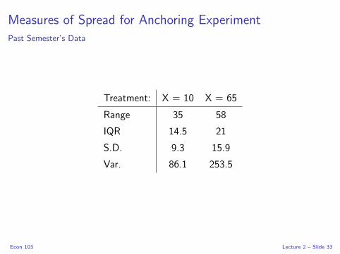
Measures of Spread for Anchoring ExperimentPast Semester’s Data
Treatment: X = 10 X = 65
Range 35 58
IQR 14.5 21
S.D. 9.3 15.9
Var. 86.1 253.5
Econ 103 Lecture 2 – Slide 33
Lecture #3 – Summary Statistics Part II
Why squares in the definition of variance?
Outliers, Skewness, & Symmetry
Sample versus Population, Empirical Rule
Centering, Standardizing, & Z-Scores
Relating Two Variables: Cross-tabs, Covariance, & Correlation
Econ 103 Lecture 3 – Slide 1

Why Squares?
s2 =1
n − 1
n∑i=1
(xi − x)2
What’s Wrong With This?
1
n − 1
N∑i=1
(xi − x) =1
n − 1
[n∑
i=1
xi −n∑
i=1
x
]=
1
n − 1
[n∑
i=1
xi − nx
]
=1
n − 1
[n∑
i=1
xi − n · 1n
n∑i=1
xi
]
=1
n − 1
[n∑
i=1
xi −n∑
i=1
xi
]= 0
Econ 103 Lecture 3 – Slide 2

Variance is Sensitive to Skewness and OutliersAnd so is Standard Deviation!
s2 =1
n − 1
n∑i=1
(xi − x)2
Outliers
Differentiate with respect to (xi − x) ⇒ the farther an observation
is from the mean, the larger its effect on the variance.
Skewness
Variance measures average squared distance from center, taking
mean as the center, but the mean is sensitive to skewness!
Econ 103 Lecture 3 – Slide 3

Skewness – A Measure of Symmetry
Skewness =1
n
∑ni=1(xi − x)3
s3
What do the values indicate?
Zero ⇒ symmetry, positive right-skewed, negative left-skewed.
Why cubed?
To get the desired sign.
Why divide by s3?
So that skewness is unitless
Rule of Thumb
Typically (but not always), right-skewed ⇒ mean > median
left-skewed ⇒ mean < median
Econ 103 Lecture 3 – Slide 4
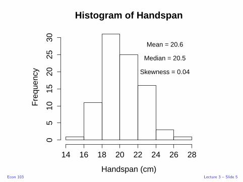
Histogram of Handspan
Handspan (cm)
Fre
quen
cy
14 16 18 20 22 24 26 28
05
1015
2025
30Mean = 20.6
Median = 20.5
Skewness = 0.04
Econ 103 Lecture 3 – Slide 5

Histogram of Handedness
Handedness
Fre
quen
cy
−1.0 −0.5 0.0 0.5 1.0
05
1015
2025
30
Mean = 0.66
Median = 0.73
Skewness = −2.26
Econ 103 Lecture 3 – Slide 6
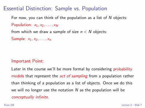
Essential Distinction: Sample vs. Population
For now, you can think of the population as a list of N objects:
Population: x1, x2, . . . , xN
from which we draw a sample of size n < N objects:
Sample: x1, x2, . . . , xn
Important Point:
Later in the course we’ll be more formal by considering probability
models that represent the act of sampling from a population rather
than thinking of a population as a list of objects. Once we do this
we will no longer use the notation N as the population will be
conceptually infinite.
Econ 103 Lecture 3 – Slide 7

Essential Distinction: Parameter vs. Statistic
N individuals in the Population, n individuals in the Sample:
Parameter (Population) Statistic (Sample)
Mean µ =1
N
N∑i=1
xi x =1
n
n∑i=1
xi
Var. σ2 =1
N
N∑i=1
(xi − µ)2 s2 =1
n − 1
n∑i=1
(xi − x)2
S.D. σ =√σ2 s =
√s2
Key Point
We use a sample x1, . . . , xn to calculate statistics (e.g. x , s2, s) that serve
as estimates of the corresponding population parameters (e.g. µ, σ2, σ).
Econ 103 Lecture 3 – Slide 8

Why Do Sample Variance and Std. Dev. Divide by n − 1?
Pop. Var. σ2 =1
N
N∑i=1
(xi − µ)2 Sample Var. s2 =1
n − 1
n∑i=1
(xi − x)2
Pop. S.D. σ =√σ2 Sample S.D. s =
√s2
There is an important reason for this, but explaining it requires
some concepts we haven’t learned yet.
Econ 103 Lecture 3 – Slide 9
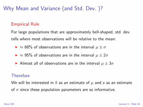
Why Mean and Variance (and Std. Dev. )?
Empirical Rule
For large populations that are approximately bell-shaped, std. dev.
tells where most observations will be relative to the mean:
I ≈ 68% of observations are in the interval µ± σ
I ≈ 95% of observations are in the interval µ± 2σ
I Almost all of observations are in the interval µ± 3σ
Therefore
We will be interested in x as an estimate of µ and s as an estimate
of σ since these population parameters are so informative.
Econ 103 Lecture 3 – Slide 10

Which is more “extreme?”
(a) Handspan of 27cm
(b) Height of 78in
Econ 103 Lecture 3 – Slide 11

Centering: Subtract the Mean
Handspan Height
27cm− 20.6cm = 6.4cm 78in− 67.6in = 10.4in
Econ 103 Lecture 3 – Slide 12

Standardizing: Divide by S.D.
Handspan Height
27cm− 20.6cm = 6.4cm 78in− 67.6in = 10.4in
6.4cm/2.2cm ≈ 2.9 10.4in/4.5in ≈ 2.3
The units have disappeared!
Econ 103 Lecture 3 – Slide 13

Z-scores: How many standard deviations from the mean?Best for Symmetric Distribution, No Outliers (Why?)
zi =xi − x
s
Unitless
Allows comparison of variables with different units.
Detecting Outliers
Measures how “extreme” one observation is relative to the others.
Linear Transformation
Econ 103 Lecture 3 – Slide 14

What is the sample mean of the z-scores?
z =1
n
n∑i=1
zi =1
n
n∑i=1
xi − x
s=
1
n · s
[n∑
i=1
xi −n∑
i=1
x
]
=1
n · s
[n∑
i=1
xi − nx
]=
1
n · s
[n∑
i=1
xi − n · 1n
n∑i=1
xi
]
=1
n · s
[n∑
i=1
xi −n∑
i=1
xi
]= 0
Econ 103 Lecture 3 – Slide 15
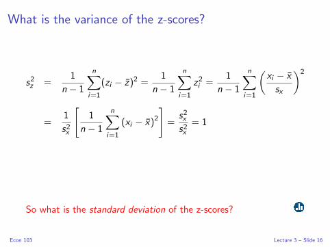
What is the variance of the z-scores?
s2z =1
n − 1
n∑i=1
(zi − z)2 =1
n − 1
n∑i=1
z2i =1
n − 1
n∑i=1
(xi − x
sx
)2
=1
s2x
[1
n − 1
n∑i=1
(xi − x)2]=
s2xs2x
= 1
So what is the standard deviation of the z-scores?
Econ 103 Lecture 3 – Slide 16

Population Z-scores and the Empirical Rule: µ± 2σ
If we knew the population mean µ and standard deviation σ we
could create a population version of a z-score. This leads to an
important way of rewriting the Empirical Rule:
Bell-shaped population ⇒ approx. 95% of observations xi satisfy
µ− 2σ ≤ xi ≤ µ+ 2σ
− 2σ ≤ xi − µ ≤ 2σ
− 2 ≤ xi − µ
σ≤ 2
Econ 103 Lecture 3 – Slide 17

Relationships Between
Variables
Econ 103 Lecture 3 – Slide 18

Crosstabs – Show Relationship between Categorical Vars.(aka Contingency Tables)
Eye Color Sex
Male Female Total
Black 5 2 7
Blue 6 4 10
Brown 26 31 57
Copper 1 0 1
Dark Brown 0 1 1
Green 4 1 5
Hazel 2 2 4
Maroon 1 0 1
Total 45 41 86
Econ 103 Lecture 3 – Slide 19

Example with Crosstab in Percents
Econ 103 Lecture 3 – Slide 20

Who Supported the Vietnam War?
Econ 103 Lecture 3 – Slide 21

Who Were the Doves?
Which group do you think was most strongly in favor of the
withdrawal of US troops from Vietnam?
(a) Adults with only a Grade School Education
(b) Adults with a High School Education
(c) Adults with a College Education
Please respond with your remote.
Econ 103 Lecture 3 – Slide 22

Who Were the Hawks?
Which group do you think was most strongly opposed to the
withdrawal of US troops from Vietnam?
(a) Adults with only a Grade School Education
(b) Adults with a High School Education
(c) Adults with a College Education
Please respond with your remote.
Econ 103 Lecture 3 – Slide 23

From The Economist –“Lexington,” October 4th, 2001
“Back in the Vietnam days, the anti-war movement
spread from the intelligentsia into the rest of the
population, eventually paralyzing the country’s will to
fight.”
Econ 103 Lecture 3 – Slide 24

Who Really Supported the Vietnam WarGallup Poll, January 1971
Econ 103 Lecture 3 – Slide 25

What about numeric data?
Econ 103 Lecture 3 – Slide 26

Covariance and Correlation: Linear Dependence Measures
Two Samples of Numeric Data
x1, . . . , xn and y1, . . . , yn
Dependence
Do x and y both tend to be large (or small) at the same time?
Key Point
Use the idea of centering and standardizing to decide what “big”
or “small” means in this context.
Econ 103 Lecture 3 – Slide 27

Notation
x =1
n
n∑i=1
xi
y =1
n
n∑i=1
yi
sx =
√√√√ 1
n − 1
n∑i=1
(xi − x)2
sy =
√√√√ 1
n − 1
n∑i=1
(yi − y)2
Econ 103 Lecture 3 – Slide 28

Covariance
sxy =1
n − 1
n∑i=1
(xi − x)(yi − y)
I Centers each observation around its mean and multiplies.
I Zero ⇒ no linear dependence
I Positive ⇒ positive linear dependence
I Negative ⇒ negative linear dependence
I Population parameter: σxy
I Units?
Econ 103 Lecture 3 – Slide 29

Correlation
rxy =1
n − 1
n∑i=1
(xi − x
sx
)(yi − y
sy
)=
sxysxsy
I Centers and standardizes each observation
I Bounded between -1 and 1
I Zero ⇒ no linear dependence
I Positive ⇒ positive linear dependence
I Negative ⇒ negative linear dependence
I Population parameter: ρxy
I Unitless
Econ 103 Lecture 3 – Slide 30

We’ll have more to say about correlation and
covariance when we discuss linear regression.
Econ 103 Lecture 3 – Slide 31

Essential Distinction: Parameter vs. StatisticAnd Population vs. Sample
N individuals in the Population, n individuals in the Sample:
Parameter (Population) Statistic (Sample)
Mean µx =1
N
N∑i=1
xi x =1
n
n∑i=1
xi
Var. σ2x =
1
N
N∑i=1
(xi − µ)2 s2x =1
n − 1
n∑i=1
(xi − x)2
S.D. σx =√σ2x sx =
√s2
Cov. σxy =
∑Ni=1(xi − µx)(yi − µy )
Nsxy =
∑ni=1(xi − x)(yi − y)
n − 1Corr. ρ =
σxy
σxσyr =
sxysxsy
Econ 103 Lecture 3 – Slide 32
Lecture #4 – Linear Regression I
Overview / Intuition for Linear Regression
Deriving the Regression Equations
Relating Regression, Covariance and Correlation
Regression to the Mean
Econ 103 Lecture 4 – Slide 1

Predict Second Midterm given 81 on First
60 70 80 90
5060
7080
9010
0
Score on Midterm 1 (%)
Sco
re o
n M
idte
rm 2
(%
)
Econ 103 Lecture 4 – Slide 2

Predict Second Midterm given 81 on First
60 70 80 90
5060
7080
9010
0
Score on Midterm 1 (%)
Sco
re o
n M
idte
rm 2
(%
)
75
Econ 103 Lecture 4 – Slide 3

But if they’d only gotten 79 we’d predict higher?!
60 70 80 90
5060
7080
9010
0
Score on Midterm 1 (%)
Sco
re o
n M
idte
rm 2
(%
)
75
87
Econ 103 Lecture 4 – Slide 4

No one who took both exams got 89 on the first!
60 70 80 90
5060
7080
9010
0
Score on Midterm 1 (%)
Sco
re o
n M
idte
rm 2
(%
)
75
87
Econ 103 Lecture 4 – Slide 5

Regression: “Best Fitting” Line Through Cloud of Points
60 70 80 90
5060
7080
9010
0
y ≈ 32 + 0.6x
Score on Midterm 1 (%)
Sco
re o
n M
idte
rm 2
(%
)
Econ 103 Lecture 4 – Slide 6

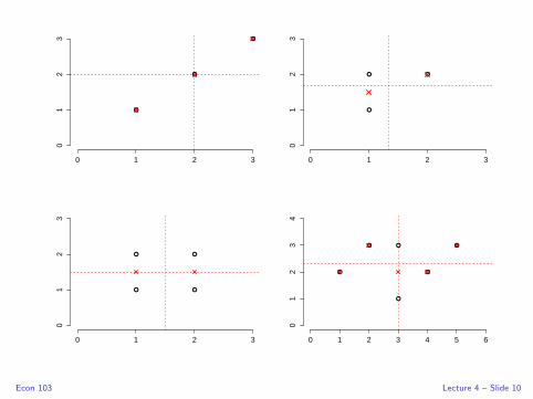
Fitting a Line by Eye
Econ 103 Lecture 4 – Slide 7

●
●
●
0 1 2 3
01
23
●
● ●
0 1 2 3
01
23
●
●
●
●
0 1 2 3
01
23
●
●
●
●
●
●
0 1 2 3 4 5 6
01
23
4
Econ 103 Lecture 4 – Slide 8

●
●
●
0 1 2 3
01
23
●
● ●
0 1 2 3
01
23
●
●
●
●
0 1 2 3
01
23
●
●
●
●
●
●
0 1 2 3 4 5 6
01
23
4
Econ 103 Lecture 4 – Slide 9
●
●
●
0 1 2 3
01
23
●
● ●
0 1 2 3
01
23
●
●
●
●
0 1 2 3
01
23
●
●
●
●
●
●
0 1 2 3 4 5 6
01
23
4
Econ 103 Lecture 4 – Slide 10

●
●
●
0 1 2 3
01
23
●
● ●
0 1 2 3
01
23
●
●
●
●
0 1 2 3
01
23
●
●
●
●
●
●
0 1 2 3 4 5 6
01
23
4
Econ 103 Lecture 4 – Slide 11

But How to Do this Formally?
Econ 103 Lecture 4 – Slide 12

Least Squares Regression – Predict Using a Line
The Prediction
Predict score y = a+ bx on 2nd midterm if you scored x on 1st
How to choose (a, b)?
Linear regression chooses the slope (b) and intercept (a) that
minimize the sum of squared vertical deviationsn∑
i=1
d2i =
n∑i=1
(yi − a− bxi )2
Why Squared Deviations?
Econ 103 Lecture 4 – Slide 13

Important Point About Notation
minimizea,b
n∑i=1
d2i =
n∑i=1
(yi − a− bxi )2
y = a+ bx
I (xi , yi )ni=1 are the observed data
I y is our prediction for a given value of x
I Neither x nor y needs to be in out dataset!
Econ 103 Lecture 4 – Slide 14

60 70 80 90
5060
7080
9010
0
∑d2 = 25596.88
y = 120 + (−0.6)x
y
Econ 103 Lecture 4 – Slide 15

60 70 80 90
5060
7080
9010
0
∑d2 = 10728
y = 80 + (0)x
y
Econ 103 Lecture 4 – Slide 16

60 70 80 90
5060
7080
9010
0
∑d2 = 8313.72
y = 58 + (0.3)x
y
Econ 103 Lecture 4 – Slide 17
60 70 80 90
5060
7080
9010
0
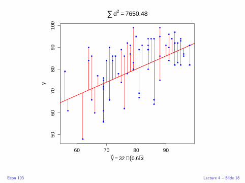
∑d2 = 7650.48
y = 32 + (0.6)x
y
Econ 103 Lecture 4 – Slide 18

Prediction given 89 on Midterm 1?
60 70 80 90
5060
7080
9010
0
y ≈ 32 + 0.6x
Score on Midterm 1 (%)
Sco
re o
n M
idte
rm 2
(%
)
32 + 0.6× 89 = 32 + 53.4 = 85.4Econ 103 Lecture 4 – Slide 19

You Need to Know How To Derive This
Minimize the sum of squared vertical deviations from the line:
mina,b
n∑i=1
(yi − a− bxi )2
How should we proceed?
(a) Differentiate with respect to x
(b) Differentiate with respect to y
(c) Differentiate with respect to x , y
(d) Differentiate with respect to a, b
(e) Can’t solve this with calculus.
Econ 103 Lecture 4 – Slide 20

Objective Function
mina,b
n∑i=1
(yi − a− bxi )2
FOC with respect to a
−2n∑
i=1
(yi − a− bxi ) = 0
n∑i=1
yi −n∑
i=1
a− bn∑
i=1
xi = 0
1
n
n∑i=1
yi −na
n− b
n
n∑i=1
xi = 0
y − a− bx = 0
Econ 103 Lecture 4 – Slide 21

Regression Line Goes Through the Means!
y = a + bx
Econ 103 Lecture 4 – Slide 22
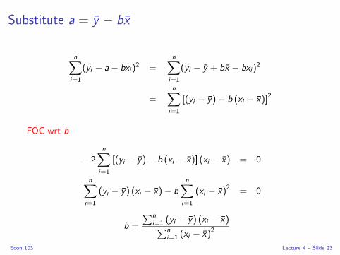
Substitute a = y − bx
n∑i=1
(yi − a− bxi )2 =
n∑i=1
(yi − y + bx − bxi )2
=n∑
i=1
[(yi − y)− b (xi − x)]2
FOC wrt b
− 2n∑
i=1
[(yi − y)− b (xi − x)] (xi − x) = 0
n∑i=1
(yi − y) (xi − x)− bn∑
i=1
(xi − x)2 = 0
b =
∑ni=1 (yi − y) (xi − x)∑n
i=1 (xi − x)2
Econ 103 Lecture 4 – Slide 23

Simple Linear Regression
Problem
mina,b
n∑i=1
(yi − a− bxi )2
Solution
b =
∑ni=1 (yi − y) (xi − x)∑n
i=1 (xi − x)2
a = y − bx
Econ 103 Lecture 4 – Slide 24
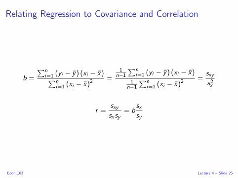
Relating Regression to Covariance and Correlation
b =
∑ni=1 (yi − y) (xi − x)∑n
i=1 (xi − x)2=
1n−1
∑ni=1 (yi − y) (xi − x)
1n−1
∑ni=1 (xi − x)2
=sxys2x
r =sxysxsy
= bsxsy
Econ 103 Lecture 4 – Slide 25

Comparing Regression, Correlation and Covariance
Units
Correlation is unitless, covariance and regression coefficients (a, b)
are not. (What are the units of these?)
Symmetry
Correlation and covariance are symmetric, regression isn’t.
(Switching x and y axes changes the slope and intercept.)
On the Homework
Regression with z-scores rather than raw data gives a = 0, b = rxy
Econ 103 Lecture 4 – Slide 26

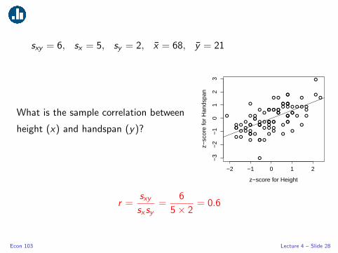
sxy = 6, sx = 5, sy = 2, x = 68, y = 21
What is the sample correlation between
height (x) and handspan (y)?●
●●
●
● ●
●
●
●
●
●
● ●
●
●
●
●
●●
●
●
●
●●
●
●
●
●
●
●
● ●
●
●
●
●
●
●●●
●
●●
●●
●
●
●
●
●
●●
●●
●
●
●
●
●●
●
●
●
●
● ●●
●
●●
●
●●
●●
●
●
●
●
●●
●
●
●
●
●
●
60 65 70 75
1416
1820
2224
26
x = Height (in)
y =
Han
dspa
n (c
m)
Econ 103 Lecture 4 – Slide 27
sxy = 6, sx = 5, sy = 2, x = 68, y = 21
What is the sample correlation between
height (x) and handspan (y)?●
●●
●
● ●
●
●
●
●
●
● ●
●
●
●
●
●●
●
●
●
●●
●
●
●
●
●
●
● ●
●
●
●
●
●
●●●
●
●●
●●
●
●
●
●
●
●●
●●
●
●
●
●
●●
●
●
●
●
● ●●
●
●●
●
●●
●●
●
●
●
●
●●
●
●
●
●
●
●
−2 −1 0 1 2
−3
−2
−1
01
23
z−score for Height
z−sc
ore
for
Han
dspa
nr =
sxysxsy
=6
5× 2= 0.6
Econ 103 Lecture 4 – Slide 28
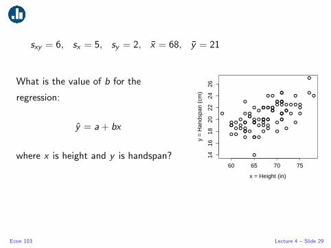
sxy = 6, sx = 5, sy = 2, x = 68, y = 21
What is the value of b for the
regression:
y = a+ bx
where x is height and y is handspan?
●●
●●
● ●
●
●
●
●
●
● ●
●
●
●
●
●●
●
●
●
●●
●
●
●
●
●
●
● ●
●
●
●
●
●
●●●
●
●●
●●
●
●
●
●
●
●●
●●
●
●
●
●
●●
●
●
●
●
● ●●
●
●●
●
●●
●●
●
●
●
●
●●
●
●
●
●
●
●
60 65 70 75
1416
1820
2224
26
x = Height (in)
y =
Han
dspa
n (c
m)
Econ 103 Lecture 4 – Slide 29

sxy = 6, sx = 5, sy = 2, x = 68, y = 21
What is the value of b for the
regression:
y = a+ bx
where x is height and y is handspan?
●●
●●
● ●
●
●
●
●
●
● ●
●
●
●
●
●●
●
●
●
●●
●
●
●
●
●
●
● ●
●
●
●
●
●
●●●
●
●●
●●
●
●
●
●
●
●●
●●
●
●
●
●
●●
●
●
●
●
● ●●
●
●●
●
●●
●●
●
●
●
●
●●
●
●
●
●
●
●
60 65 70 75
1416
1820
2224
26
x = Height (in)
y =
Han
dspa
n (c
m)
b =sxys2x
=6
52= 6/25 = 0.24
Econ 103 Lecture 4 – Slide 30

sxy = 6, sx = 5, sy = 2, x = 68, y = 21
What is the value of a for the
regression:
y = a+ bx
where x is height and y is handspan?
(prev. slide b = 0.24)
●●
●●
● ●
●
●
●
●
●
● ●
●
●
●
●
●●
●
●
●
●●
●
●
●
●
●
●
● ●
●
●
●
●
●
●●●
●
●●
●●
●
●
●
●
●
●●
●●
●
●
●
●
●●
●
●
●
●
● ●●
●
●●
●
●●
●●
●
●
●
●
●●
●
●
●
●
●
●
60 65 70 75
1416
1820
2224
26
x = Height (in)
y =
Han
dspa
n (c
m)
Econ 103 Lecture 4 – Slide 31

sxy = 6, sx = 5, sy = 2, x = 68, y = 21
What is the value of a for the
regression:
y = a+ bx
where x is height and y is handspan?
(prev. slide b = 0.24)
●●
●●
● ●
●
●
●
●
●
● ●
●
●
●
●
●●
●
●
●
●●
●
●
●
●
●
●
● ●
●
●
●
●
●
●●●
●
●●
●●
●
●
●
●
●
●●
●●
●
●
●
●
●●
●
●
●
●
● ●●
●
●●
●
●●
●●
●
●
●
●
●●
●
●
●
●
●
●
60 65 70 75
1416
1820
2224
26
x = Height (in)
y =
Han
dspa
n (c
m)
a = y − bx = 21− 0.24× 68 = 4.68
Econ 103 Lecture 4 – Slide 32

sxy = 6, sy = 5, sx = 2, y = 68, x = 21
What is the value of b for the
regression:
y = a+ bx
where x is handspan and y is height?
●
●●
●
●
●
●
●
●
●
●
●●
●
●
●
●
●
●
●
●
●
●
●
●
● ●●
●
●
●
●
●
●●
●
●●●
●
●
●
●
●
●
●
●
●
●
●
●
●
●●
●
●
●
● ●
●
●
●
●
●
●
●
●
●
●
●
●
●
●
●
●
●
●
●
●
●
●
●
●
●●
●
●
14 16 18 20 22 24 26
6065
7075
x = Handspan (cm)
y =
Hei
ght (
in)
Econ 103 Lecture 4 – Slide 33

sxy = 6, sy = 5, sx = 2, y = 68, x = 21
What is the value of b for the
regression:
y = a+ bx
where x is handspan and y is height?
●
●●
●
●
●
●
●
●
●
●
●●
●
●
●
●
●
●
●
●
●
●
●
●
● ●●
●
●
●
●
●
●●
●
●●●
●
●
●
●
●
●
●
●
●
●
●
●
●
●●
●
●
●
● ●
●
●
●
●
●
●
●
●
●
●
●
●
●
●
●
●
●
●
●
●
●
●
●
●
●●
●
●
14 16 18 20 22 24 26
6065
7075
x = Handspan (cm)
y =
Hei
ght (
in)
b =sxys2x
= 6/22 = 1.5
Econ 103 Lecture 4 – Slide 34

EXTREMELY IMPORTANT
I Regression, Covariance and Correlation: linear association.
I Linear association 6= causation.
I Linear is not the only kind of association!
●
●
●
●
●
●
●
●
●● ● ●
●
●
●
●
●
●
●
●
●
−1.0 −0.5 0.0 0.5 1.0
0.0
0.2
0.4
0.6
0.8
1.0
Correlation = 0
x
y
Econ 103 Lecture 4 – Slide 35
Regression to the Mean and the Regression Fallacy
Please read Chapter 17 of “Thinking Fast and Slow” by Daniel
Kahnemann which I have posted on Piazza. This reading is fair
game on an exam or quiz.
Econ 103 Lecture 4 – Slide 36

●
● ●
●
● ● ●●
●
●
● ●●
● ●
●●
●
●●
●●
●●
●●●
●
●● ●●
●
●
●●
● ● ●
●●
●●
●●
●●
●
●
●
●● ●
●● ●
●
●●
●●
● ●●
●●●●
● ●●
●●
●
●●● ●●
●●
●●
●
●●●
●●
●●
●
●
●●
●
●●
●
●●
●
●
● ●
●
● ●●
●
●● ●
●●
●
● ●●●
●●
●●●
●
●
●●●
●
● ● ●
●●●
●● ●
●
●●●
●
●● ●●
● ●●●
● ●
●
● ●
●
●
●●
●●
●
●●
●●
●●
●●●
●
●●
●
●
●
● ●●
●● ●
●●●
●● ●
●
●
●●
● ●
● ● ●
●●
●
●
●
●
●
●
●
●
●
●
●
●
●
●
● ●
●
● ●
●
●
● ●
● ●
●
●●●
● ●
●
●
●
● ●
● ●● ● ●●●
●●
●
●
●●
●
●
● ●
●●
● ●●
●
●
●
●●
● ●●
●
●●
●●
●
●●●●
●●
●●● ●
●
●
● ●
● ● ●● ● ●
●●
●●
● ●
● ●●
●● ●
●
●●
●●
●●●
●●
●●●
●●
●
●
● ●●
●●
●
●● ● ●
●
●● ●●
●●●
●
●●
● ●●●
● ● ●●● ●
●
●●●
●● ●
●
●●
● ●●
●
●
●● ●
●
●●
●●
●● ●●
●● ● ●●
●●
● ●
●●
● ● ●●
●● ●
●
●● ●
●●
●●●
● ●
●
●
●
●
●●
●
●
●
●
●
●
●
●
●
●
●
●
●
●
●
●●
●
●● ●
●●
●
●
●
●
●●●
●● ● ●
●
●● ●●
●●
●●●
●
●
●
●●● ●●●
●●
●
●
●●
●
●
●
●
●●●
●●●●
● ●●
●●●●●● ● ●
●●
●●
●
●
●●●●
●
●●●
● ●●●●
●● ●
●●●
●
●●●●
●
●●
●
● ●●
●● ●
●
●●●
●●● ●●
●●●
●●●
●●●
●●
●●
●
●
●
●
●●
●●
●
●●●
●
●
●
●
●●
●
●●
● ●
●●
●
●
●
● ● ● ●●
●●
●●
●
●● ●●
●
●● ●
●
●
● ●
●● ●
●
●●
● ●
●
●
● ●● ●
●
● ●
●
●
●●●
●●
●
●
●
●
●●
●
●
●
●
●
●
●
●
●
● ●●
●
●
●●
●●
●●●
●
● ●●
●●
●
●●
●● ●● ● ●
●
●●●
●●
●
● ●
● ● ●
● ● ● ●
●
●
●
●
●
●● ● ●●●
● ●
● ●●
●
●●● ●●
●●
●
●●
●●●
●●
●● ●●● ●
●●●
●● ●
●
● ●
●
●
●●●
● ●●
●
●●● ●
● ●●●
●
●●
●●●
●●
● ●
●
● ●
● ●
●
●●● ●
●●
●
●
● ●●
●
●●
●●
●
●●●●●
● ●●
●
● ●●●● ●
●●
●
●
● ●●
●●●●
●
●
●
●
● ●●●
●
●
●● ● ●
●●
● ●
●
●●
●
●●
●
● ●
●
●●
●●
●
●
●
●
●
●
●
●
●
●
●
●
●
●
●
●
●●
●● ● ● ●
●●
●
●
●●●
●●
●
● ●
● ●
●
●● ●
● ●●● ●●●
●●
●● ●
●
● ●●
● ●●●
●
●
●
●
●
●●●
●
●
●
●●●
●
●
●
●● ● ●●● ●
●●
●●
●●
●
●●●●● ●
●●
●●
●●●
●
●● ●● ●●
●●●
●●
● ●●
●
●● ●
● ●●●
●●●
●●
●●●
●●●●
●
●●
●
●●
●● ●
●
●
●●
● ●
●
●●
●● ● ●
● ●●
●●●
●● ●
● ●
●
●●●
●●●
● ●●●
●●●
●●
●
●
●●
●
●
● ●
●●
●●
●●●
● ●
●●
●
●●
●
●
● ● ● ●
●
●
●
●
●
●
●
●
●
●
●
●●
●
60 65 70 75
6065
7075
Pearson Dataset
Height of Father (in)
Hei
ght o
f Son
(in
)
Econ 103 Lecture 4 – Slide 37

Regression to the Mean
Skill and Luck / Genes and Random Environmental Factors
Unless rxy = 1, There Is Regression to the Mean
y − y
sy= rxy
x − x
sx
Least-squares Prediction y closer to y than x is to x
You will derive the above formula in this week’s homework.
Econ 103 Lecture 4 – Slide 38

Lecture #5 – Basic Probability I
Probability as Long-run Relative Frequency
Sets, Events and Axioms of Probability
“Classical” Probability
Econ 103 Lecture 5 – Slide 1

Our Definition of Probability for this Course
Probability = Long-run Relative Frequency
That is, relative frequencies settle down to probabilities if we carry
out an experiment over, and over, and over...
Econ 103 Lecture 5 – Slide 2

0.00
0.10
0.20
0.30
Random Die Rolls
n = 10
Rel
ativ
e F
requ
ency
1 2 4 5 6
Econ 103 Lecture 5 – Slide 3

0.00
0.10
0.20
0.30
Random Die Rolls
n = 50
Rel
ativ
e F
requ
ency
1 2 3 4 5 6
Econ 103 Lecture 5 – Slide 4

0.00
0.05
0.10
0.15
Random Die Rolls
n = 1000
Rel
ativ
e F
requ
ency
1 2 3 4 5 6
Econ 103 Lecture 5 – Slide 5

0.00
0.05
0.10
0.15
Random Die Rolls
n = 1,000,000
Rel
ativ
e F
requ
ency
1 2 3 4 5 6
Econ 103 Lecture 5 – Slide 6

What do you think of this argument?
I The probability of flipping heads is 1/2: if we flip a coin many
times, about half of the time it will come up heads.
I The last ten throws in a row the coin has come up heads.
I The coin is bound to come up tails next time – it would be
very rare to get 11 heads in a row.
(a) Agree
(b) Disagree
Econ 103 Lecture 5 – Slide 7

The Gambler’s Fallacy
Relative frequencies settle down to probabilities, but this does
not mean that the trials are dependent.
Dependent = “Memory” of Prev. Trials
Independent = No “Memory” of Prev. Trials
Econ 103 Lecture 5 – Slide 8

Terminology
Random Experiment
An experiment whose outcomes are random.
Basic Outcomes
Possible outcomes (mutually exclusive) of random experiment.
Sample Space: S
Set of all basic outcomes of a random experiment.
Event: E
A subset of the Sample Space (i.e. a collection of basic outcomes).
In set notation we write E ⊆ S .
Econ 103 Lecture 5 – Slide 9
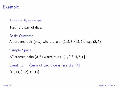
Example
Random Experiment
Tossing a pair of dice.
Basic Outcome
An ordered pair (a, b) where a, b ∈ {1, 2, 3, 4, 5, 6}, e.g. (2, 5)
Sample Space: S
All ordered pairs (a, b) where a, b ∈ {1, 2, 3, 4, 5, 6}
Event: E = {Sum of two dice is less than 4}{(1, 1), (1, 2), (2, 1)}
Econ 103 Lecture 5 – Slide 10

Visual Representation
E
S
O1
O2
O3
Econ 103 Lecture 5 – Slide 11
Probability is Defined on Sets,
and Events are Sets
Econ 103 Lecture 5 – Slide 12

Complement of an Event: Ac = not A
A
S
Figure: The complement Ac of an event A ⊆ S is the collection of all
basic outcomes from S not contained in A.
Econ 103 Lecture 5 – Slide 13

Intersection of Events: A ∩ B = A and B
A B
S
Figure: The intersection A∩B of two events A,B ⊆ S is the collection of
all basic outcomes from S contained in both A and B
Econ 103 Lecture 5 – Slide 14

Union of Events: A ∪ B = A or B
A B
S
Figure: The union A ∪ B of two events A,B ⊆ S is the collection of all
basic outcomes from S contained in A, B or both.
Econ 103 Lecture 5 – Slide 15
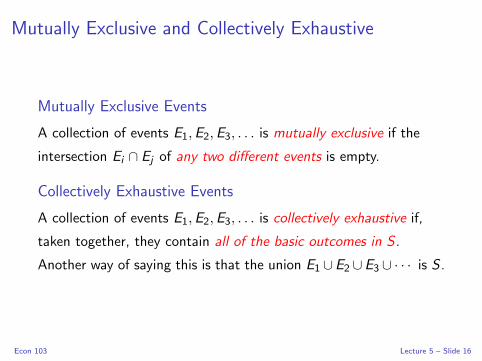
Mutually Exclusive and Collectively Exhaustive
Mutually Exclusive Events
A collection of events E1,E2,E3, . . . is mutually exclusive if the
intersection Ei ∩ Ej of any two different events is empty.
Collectively Exhaustive Events
A collection of events E1,E2,E3, . . . is collectively exhaustive if,
taken together, they contain all of the basic outcomes in S .
Another way of saying this is that the union E1 ∪E2 ∪E3 ∪ · · · is S .
Econ 103 Lecture 5 – Slide 16

Implications
Mutually Exclusive Events
If one of the events occurs, then none of the others did.
Collectively Exhaustive Events
One of these events must occur.
Econ 103 Lecture 5 – Slide 17

Mutually Exclusive but not Collectively Exhaustive
A
B
S
Figure: Although A and B don’t overlap, they also don’t cover S .
Econ 103 Lecture 5 – Slide 18

Collectively Exhaustive but not Mutually Exclusive
A B C
D
S
Figure: Together A,B,C and D cover S , but D overlaps with B and C .
Econ 103 Lecture 5 – Slide 19
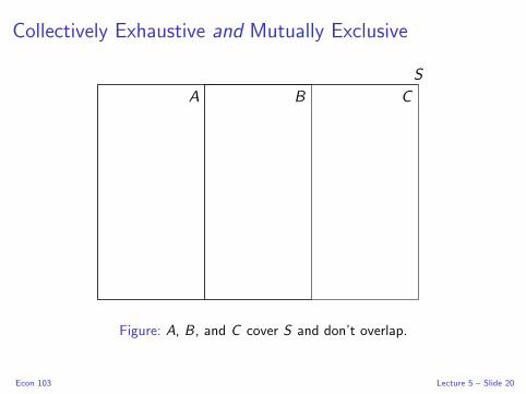
Collectively Exhaustive and Mutually Exclusive
A B C
S
Figure: A, B, and C cover S and don’t overlap.
Econ 103 Lecture 5 – Slide 20

Axioms of Probability
We assign every event A in the sample space S a real number
P(A) called the probability of A such that:
Axiom 1 0 ≤ P(A) ≤ 1
Axiom 2 P(S) = 1
Axiom 3 If A1,A2,A3, . . . are mutually exclusive events, then
P(A1∪A2∪A3∪· · · ) = P(A1)+P(A2)+P(A3)+ . . .
Econ 103 Lecture 5 – Slide 21

“Classical” Probability
When all of the basic outcomes are equally likely, calculating the
probability of an event is simply a matter of counting – count up
all the basic outcomes that make up the event, and divide by the
total number of basic outcomes.
Econ 103 Lecture 5 – Slide 22
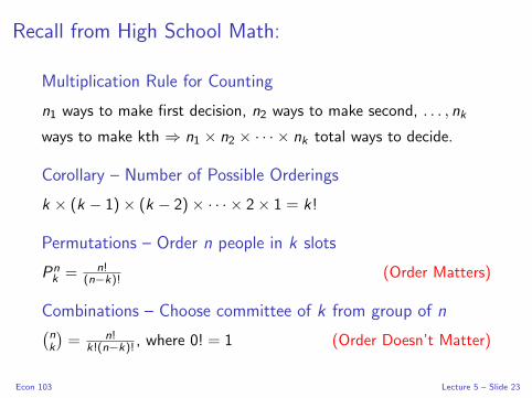
Recall from High School Math:
Multiplication Rule for Counting
n1 ways to make first decision, n2 ways to make second, . . . , nk
ways to make kth ⇒ n1 × n2 × · · · × nk total ways to decide.
Corollary – Number of Possible Orderings
k × (k − 1)× (k − 2)× · · · × 2× 1 = k!
Permutations – Order n people in k slots
Pnk = n!
(n−k)! (Order Matters)
Combinations – Choose committee of k from group of n(nk
)= n!
k!(n−k)! , where 0! = 1 (Order Doesn’t Matter)
Econ 103 Lecture 5 – Slide 23
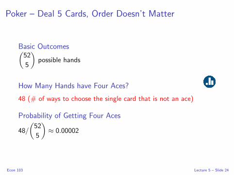
Poker – Deal 5 Cards, Order Doesn’t Matter
Basic Outcomes(52
5
)possible hands
How Many Hands have Four Aces?
48 (# of ways to choose the single card that is not an ace)
Probability of Getting Four Aces
48/
(52
5
)≈ 0.00002
Econ 103 Lecture 5 – Slide 24
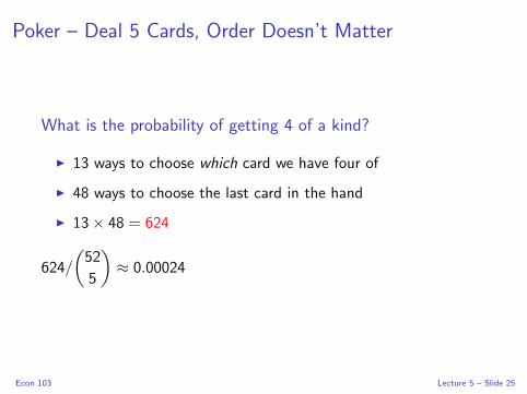
Poker – Deal 5 Cards, Order Doesn’t Matter
What is the probability of getting 4 of a kind?
I 13 ways to choose which card we have four of
I 48 ways to choose the last card in the hand
I 13× 48 = 624
624/
(52
5
)≈ 0.00024
Econ 103 Lecture 5 – Slide 25

A Fairly Ridiculous Example
Roger Federer and Novak Djokovic have agreed to play in a tennis
tournament against six Penn professors. Each player in the
tournament is randomly allocated to one of the eight rungs in the
ladder (next slide). Federer always beats Djokovic and, naturally,
either of the two pros always beats any of the professors. What is
the probability that Djokovic gets second place in the tournament?
Econ 103 Lecture 5 – Slide 26
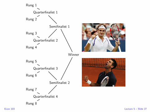
Winner
Semifinalist 2
Quarterfinalist 4
Rung 8
Rung 7
Quarterfinalist 3
Rung 6
Rung 5
Semifinalist 1
Quarterfinalist 2
Rung 4
Rung 3
Quarterfinalist 1
Rung 2
Rung 1
Econ 103 Lecture 5 – Slide 27

Solution: Order Matters!
Denominator
8! basic outcomes – ways to arrange players on tournament ladder.
Numerator
Sequence of three decisions:
1. Which rung to put Federer on? (8 possibilities)
2. Which rung to put Djokovic on?
I For any given rung that Federer is on, only 4 rungs prevent
Djokovic from meeting him until the final.
3. How to arrange the professors? (6! ways)
8× 4× 6!
8!=
8× 4
7× 8= 4/7 ≈ 0.57
Econ 103 Lecture 5 – Slide 28

Lecture #6 – Basic Probability II
Complement Rule, Logical Consequence Rule, Addition Rule
Conditional Probability
Independence, Multiplication Rule
Law of Total Probability
Prediction Markets, “Dutch Book”
Econ 103 Lecture 6 – Slide 1
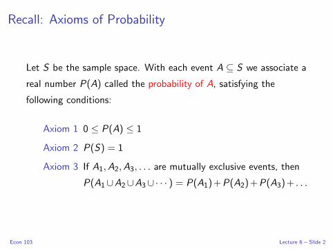
Recall: Axioms of Probability
Let S be the sample space. With each event A ⊆ S we associate a
real number P(A) called the probability of A, satisfying the
following conditions:
Axiom 1 0 ≤ P(A) ≤ 1
Axiom 2 P(S) = 1
Axiom 3 If A1,A2,A3, . . . are mutually exclusive events, then
P(A1∪A2∪A3∪· · · ) = P(A1)+P(A2)+P(A3)+ . . .
Econ 103 Lecture 6 – Slide 2

The Complement Rule: P(Ac) = 1− P(A)
Since A,Ac are mutually exclusive and
collectively exhaustive:
P(A ∪ Ac) = P(A) + P(Ac) = P(S) = 1
Rearranging:
P(Ac) = 1− P(A)
Ac
A
S
Figure: A ∩ Ac = ∅,A ∪ Ac = S
Econ 103 Lecture 6 – Slide 3

Another Important Rule – Equivalent Events
If A and B are Logically Equivalent, then P(A) = P(B).
In other words, if A and B contain exactly the same basic
outcomes, then P(A) = P(B).
Although this seems obvious it’s important to keep in mind. . .
Econ 103 Lecture 6 – Slide 4

The Logical Consequence Rule
If B Logically Entails A, then P(B) ≤ P(A)
For example, the probability that someone comes from Texas
cannot exceed the probability that she comes from the USA.
In Set Notation
B ⊆ A ⇒ P(B) ≤ P(A)
Why is this so?
If B ⊆ A, then all the basic outcomes in B are also in A.
Econ 103 Lecture 6 – Slide 5

Proof of Logical Consequence Rule (Optional)Proof won’t be on a quiz or exam but is good practice with probability axioms.
Since B ⊆ A, we have B = A ∩ B and
A = B ∪ (A ∩ Bc). Combining these,
A = (A ∩ B) ∪ (A ∩ Bc)
Now since (A ∩ B) ∩ (A ∩ Bc) = ∅,
P(A) = P(A ∩ B) + P(A ∩ Bc)
= P(B) + P(A ∩ Bc)
≥ P(B)
because 0 ≤ P(A ∩ Bc) ≤ 1.
A
B
S
Figure:
B = A ∩ B, and
A = B ∪ (A ∩ Bc)
Econ 103 Lecture 6 – Slide 6

“Odd Question” # 2
Pia is thirty-one years old, single, outspoken, and smart. She was a philosophy
major. When a student, she was an ardent supporter of Native American rights,
and she picketed a department store that had no facilities for nursing mothers.
Rank the following statements in order from most probable to least probable.
(A) Pia is an active feminist.
(B) Pia is a bank teller.
(C) Pia works in a small bookstore.
(D) Pia is a bank teller and an active feminist.
(E) Pia is a bank teller and an active feminist who takes yoga classes.
(F) Pia works in a small bookstore and is an active feminist who takes yoga
classes.
Econ 103 Lecture 6 – Slide 7

Using the Logical Consequence Rule...
(A) Pia is an active feminist.
(B) Pia is a bank teller.
(C) Pia works in a small bookstore.
(D) Pia is a bank teller and an active feminist.
(E) Pia is a bank teller and an active feminist who takes yoga classes.
(F) Pia works in a small bookstore and is an active feminist who takes yoga
classes.
Any Correct Ranking Must Satisfy:
P(A) ≥ P(D) ≥ P(E)
P(B) ≥ P(D) ≥ P(E)
P(A) ≥ P(F)
P(C) ≥ P(F)Econ 103 Lecture 6 – Slide 8

Throw a Fair Die Once
E = roll an even number
What are the basic outcomes?
{1, 2, 3, 4, 5, 6}
What is P(E )?
E = {2, 4, 6} and the basic outcomes are equally likely (and
mutually exclusive), so
P(E ) = 1/6 + 1/6 + 1/6 = 3/6 = 1/2
Econ 103 Lecture 6 – Slide 9
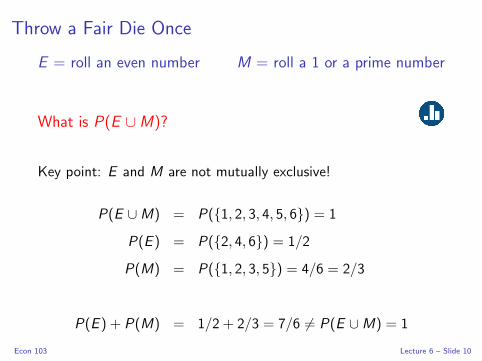
Throw a Fair Die Once
E = roll an even number M = roll a 1 or a prime number
What is P(E ∪M)?
Key point: E and M are not mutually exclusive!
P(E ∪M) = P({1, 2, 3, 4, 5, 6}) = 1
P(E ) = P({2, 4, 6}) = 1/2
P(M) = P({1, 2, 3, 5}) = 4/6 = 2/3
P(E ) + P(M) = 1/2 + 2/3 = 7/6 6= P(E ∪M) = 1
Econ 103 Lecture 6 – Slide 10
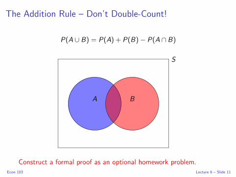
The Addition Rule – Don’t Double-Count!
P(A ∪ B) = P(A) + P(B)− P(A ∩ B)
A B
S
Construct a formal proof as an optional homework problem.
Econ 103 Lecture 6 – Slide 11

Who’s on the other side?
Econ 103 Lecture 6 – Slide 12

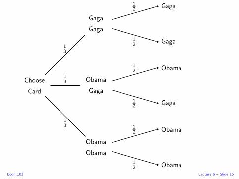
Three Cards, Each with a Face on the Front and Back
1. Gaga/Gaga
2. Obama/Gaga
3. Obama/Obama
I draw a card at random and look at one side: it’s Obama.
What is the probability that the other side is also Obama?
Econ 103 Lecture 6 – Slide 13

Let’s Try The Method of Monte Carlo...When you don’t know how to calculate, simulate.
Procedure
1. Close your eyes and thoroughly shuffle your cards.
2. Keeping eyes closed, draw a card and place it on your desk.
3. Stand if Obama is face-up on your chosen card.
4. We’ll count those standing and call the total N
5. Of those standing, sit down if Obama is not on the back of
your chosen card.
6. We’ll count those still standing and call the total m.
Monte Carlo Approximation of Desired Probability =m
N
Econ 103 Lecture 6 – Slide 14
Choose
Card
Obama
Obama
Obama12
Obama12
13
Obama
Gaga
Gaga12
Obama12
13
Gaga
Gaga
Gaga12
Gaga12
13
Econ 103 Lecture 6 – Slide 15

Conditional Probability – Reduced Sample SpaceSet of relevant outcomes restricted by condition
P(A|B) = P(A ∩ B)
P(B), provided P(B) > 0
A B
S
Figure: B becomes the “new sample space” so we need to re-scale by
P(B) to keep probabilities between zero and one.Econ 103 Lecture 6 – Slide 16

Who’s on the other side?
Let F be the event that Obama is on the front of the card of the
card we draw and B be the event that he is on the back.
P(B|F ) = P(B ∩ F )
P(F )=
1/3
1/2= 2/3
Econ 103 Lecture 6 – Slide 17

Conditional Versions of Probability Axioms
1. 0 ≤ P(A|B) ≤ 1
2. P(B|B) = 1
3. If A1,A2,A3, . . . are mutually exclusive given B, then
P(A1 ∪ A2 ∪ A3 ∪ · · · |B) = P(A1|B) + P(A2|B) + P(A3|B) . . .
Conditional Versions of Other Probability Rules
I P(A|B) = 1− P(Ac |B)
I A1 logically equivalent to A2 ⇐⇒ P(A1|B) = P(A2|B)
I A1 ⊆ A2 =⇒ P(A1|B) ≤ P(A2|B)
I P(A1 ∪ A2|B) = P(A1|B) + P(A2|B)− P(A1 ∩ A2|B)
However: P(A|B) 6= P(B|A) and P(A|Bc) 6= 1− P(A|B)!Econ 103 Lecture 6 – Slide 18

Independence and The Multiplication Rule
The Multiplication Rule
Rearrange the definition of conditional probability:
P(A ∩ B) = P(A|B)P(B)
Statistical Independence
P(A ∩ B) = P(A)P(B)
By the Multiplication Rule
Independence ⇐⇒ P(A|B) = P(A)
Interpreting Independence
Knowledge that B has occurred tells nothing about whether A will.
Econ 103 Lecture 6 – Slide 19

Will Having 5 Children Guarantee a Boy?
A couple plans to have five children. Assuming that each birth is
independent and male and female children are equally likely, what
is the probability that they have at least one boy?
By Independence and the Complement Rule,
P(no boys) = P(5 girls)
= 1/2× 1/2× 1/2× 1/2× 1/2
= 1/32
P(at least 1 boy) = 1− P(no boys)
= 1− 1/32 = 31/32 = 0.97
Econ 103 Lecture 6 – Slide 20
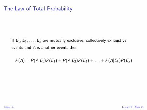
The Law of Total Probability
If E1,E2, . . . ,Ek are mutually exclusive, collectively exhaustive
events and A is another event, then
P(A) = P(A|E1)P(E1) + P(A|E2)P(E2) + . . .+ P(A|Ek)P(Ek)
Econ 103 Lecture 6 – Slide 21
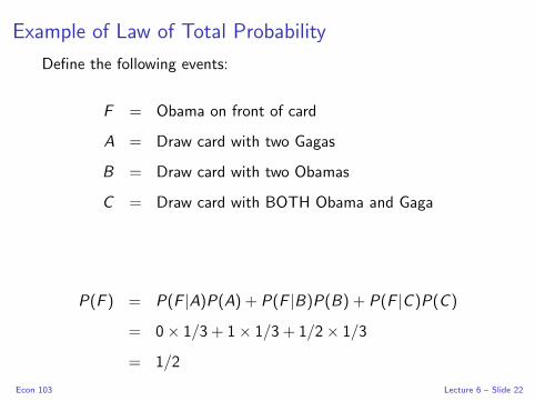
Example of Law of Total Probability
Define the following events:
F = Obama on front of card
A = Draw card with two Gagas
B = Draw card with two Obamas
C = Draw card with BOTH Obama and Gaga
P(F ) = P(F |A)P(A) + P(F |B)P(B) + P(F |C )P(C )
= 0× 1/3 + 1× 1/3 + 1/2× 1/3
= 1/2
Econ 103 Lecture 6 – Slide 22
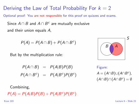
Deriving the Law of Total Probability For k = 2Optional proof: You are not responsible for this proof on quizzes and exams.
Since A ∩ B and A ∩ Bc are mutually exclusive
and their union equals A,
P(A) = P(A ∩ B) + P(A ∩ Bc)
But by the multiplication rule:
P(A ∩ B) = P(A|B)P(B)
P(A ∩ Bc) = P(A|Bc)P(Bc)
Combining,
P(A) = P(A|B)P(B) + P(A|Bc)P(Bc)
B A
S
Figure:
A = (A∩B)∪(A∩Bc),
(A∩B)∩(A∩Bc) = ∅
Econ 103 Lecture 6 – Slide 23

How do prediction markets work?
To learn more, see Wolfers & Zitzewitz (2004)
This certificate entitles the
bearer to $1 if the Patriots win
the 2016-2017 Superbowl.
Buyers – Purchase Right to Collect
Patriots very likely to win ⇒ buy for close to $1.
Patriots very unlikely to win ⇒ buy for close to $0.
Sellers – Sell Obligation to Pay
Patriots very likely to win ⇒ sell for close to $1.
Patriots very unlikely to win ⇒ sell for close to $0.
Econ 103 Lecture 6 – Slide 24

Probabilities from Beliefs
Market price of contract encodes market participants’ beliefs in the
form of probability:
Price/Payout ≈ Subjective Probability
“Dutch Book”
If the probabilities implied by prediction market prices violate any
of our probability rules there is a pure arbitrage opportunity: a way
make to make a guaranteed, risk-free profit.
Econ 103 Lecture 6 – Slide 25

A Real-world Dutch BookCourtesy of Eric Crampton
November 5th, 2012
I $2.30 for contract paying $10 if Romney wins on BetFair
I $6.58 for contract paying $10 if Obama wins on InTrade
Implied Probabilities
I BetFair: P(Romney) ≈ 0.23
I InTrade: P(Obama) ≈ 0.66
What’s Wrong with This?
Violates complement rule! P(Obama) = 1− P(Romney) but the
implied probabilities here don’t sum up to one!Econ 103 Lecture 6 – Slide 26

A Real-world Dutch BookCourtesy of Eric Crampton
November 5th, 2012
I $2.30 for contract paying $10 if Romney wins on BetFair
I $6.58 for contract paying $10 if Obama wins on InTrade
Arbitrage Strategy
Buy Equal Numbers of Each
I Cost = $2.30 + $6.58 =$8.88 per pair
I Payout if Romney Wins: $10
I Payout if Obama Wins: $10
I Guaranteed Profit: $10 - $8.88 = $1.12 per pair
Econ 103 Lecture 6 – Slide 27
Lecture #7 – Basic Probability III / Discrete RVs I
Bayes’ Rule and the Base Rate Fallacy
Overview of Random Variables
Probability Mass Functions
Econ 103 Lecture 7 – Slide 1

Four Volunteers Please!
Econ 103 Lecture 7 – Slide 2
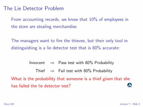
The Lie Detector Problem
From accounting records, we know that 10% of employees in
the store are stealing merchandise.
The managers want to fire the thieves, but their only tool in
distinguishing is a lie detector test that is 80% accurate:
Innocent ⇒ Pass test with 80% Probability
Thief ⇒ Fail test with 80% Probability
What is the probability that someone is a thief given that she
has failed the lie detector test?
Econ 103 Lecture 7 – Slide 3
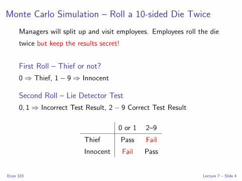
Monte Carlo Simulation – Roll a 10-sided Die Twice
Managers will split up and visit employees. Employees roll the die
twice but keep the results secret!
First Roll – Thief or not?
0 ⇒ Thief, 1− 9 ⇒ Innocent
Second Roll – Lie Detector Test
0, 1 ⇒ Incorrect Test Result, 2− 9 Correct Test Result
0 or 1 2–9
Thief Pass Fail
Innocent Fail Pass
Econ 103 Lecture 7 – Slide 4
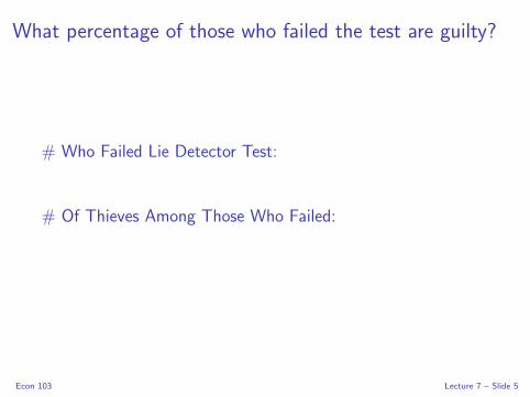
What percentage of those who failed the test are guilty?
# Who Failed Lie Detector Test:
# Of Thieves Among Those Who Failed:
Econ 103 Lecture 7 – Slide 5

Base Rate Fallacy – Failure to Consider Prior Information
Base Rate – Prior Information
Before the test we know that 10% of Employees are stealing.
People tend to focus on the fact that the test is 80% accurate
and ignore the fact that only 10% of the employees are theives.
Econ 103 Lecture 7 – Slide 6
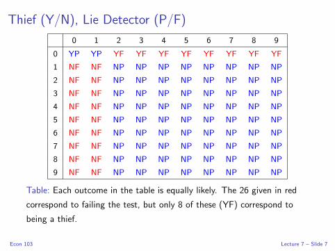
Thief (Y/N), Lie Detector (P/F)
0 1 2 3 4 5 6 7 8 9
0 YP YP YF YF YF YF YF YF YF YF
1 NF NF NP NP NP NP NP NP NP NP
2 NF NF NP NP NP NP NP NP NP NP
3 NF NF NP NP NP NP NP NP NP NP
4 NF NF NP NP NP NP NP NP NP NP
5 NF NF NP NP NP NP NP NP NP NP
6 NF NF NP NP NP NP NP NP NP NP
7 NF NF NP NP NP NP NP NP NP NP
8 NF NF NP NP NP NP NP NP NP NP
9 NF NF NP NP NP NP NP NP NP NP
Table: Each outcome in the table is equally likely. The 26 given in red
correspond to failing the test, but only 8 of these (YF) correspond to
being a thief.
Econ 103 Lecture 7 – Slide 7
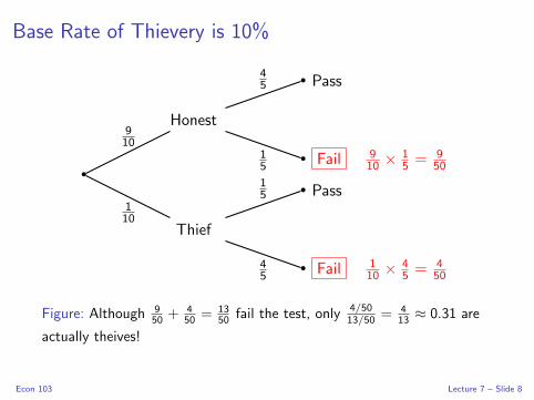
Base Rate of Thievery is 10%
Thief
Fail 110 × 4
5 = 450
45
Pass15
110
Honest
Fail 910 × 1
5 = 950
15
Pass45
910
Figure: Although 950 + 4
50 = 1350 fail the test, only 4/50
13/50 = 413 ≈ 0.31 are
actually theives!
Econ 103 Lecture 7 – Slide 8

Deriving Bayes’ Rule
Intersection is symmetric: A∩B = B ∩A so P(A∩B) = P(B ∩A)
By the definition of conditional probability,
P(A|B) = P(A ∩ B)
P(B)
And by the multiplication rule:
P(B ∩ A) = P(B|A)P(A)
Finally, combining these
P(A|B) = P(B|A)P(A)P(B)
Econ 103 Lecture 7 – Slide 9

Understanding Bayes’ Rule
P(A|B) = P(B|A)P(A)P(B)
Reversing the Conditioning
Express P(A|B) in terms of P(B|A). Relative magnitudes of the
two conditional probabilities determined by the ratio P(A)/P(B).
Base Rate
P(A) is called the “base rate” or the “prior probability.”
Denominator
Typically, we calculate P(B) using the law of toal probability
Econ 103 Lecture 7 – Slide 10

In General P(A|B) 6= P(B |A)
Question
Most college students are Democrats. Does it follow that most
Democrats are college students? (A = YES, B = NO)
Answer
There are many more Democracts than college students:
P(Dem) > P(Student)
so P(Student|Dem) is small even though P(Dem|Student) is large.
Econ 103 Lecture 7 – Slide 11

Solving the Lie Detector Problem with Bayes’ Rule
T = Employee is a Thief, F = Employee Fails Lie Detector Test
P(T |F ) = P(F |T )P(T )
P(F )
P(F ) = P(F |T )P(T ) + P(F |T c)P(T c)
= 0.8× 0.1 + 0.2× 0.9
= 0.08 + 0.18 = 0.26
P(T |F ) = 0.08
0.26=
8
26=
4
13≈ 0.31
Econ 103 Lecture 7 – Slide 12
Random Variables
Econ 103 Lecture 7 – Slide 13

Random Variables
A random variable is neither random nor a variable.
Random Variable (RV): X
A fixed function that assigns a number to each basic outcome of a
random experiment.
Realization: x
A particular numeric value that an RV could take on. We write
{X = x} to refer to the event that the RV X took on the value x .
Support Set (aka Support)
The set of all possible realizations of a RV.
Econ 103 Lecture 7 – Slide 14

Random Variables (continued)
Notation
Capital latin letters for RVs, e.g. X ,Y ,Z , and the corresponsing
lowercase letters for their realizations, e.g. x , y , z .
Intuition
You can think of an RV as a machine that spits out random
numbers: although the machine is deterministic, its inputs, the
outcomes of a random experiment, are not.
Econ 103 Lecture 7 – Slide 15

Example: Coin Flip Random Variable
S R
Tails 0
Heads 1
Figure: This random variable assigns numeric values to the random
experiment of flipping a fair coin once: Heads is assigned 1 and Tails 0.
Econ 103 Lecture 7 – Slide 16

Which of these is a realization of the Coin Flip RV?
(a) Tails
(b) 2
(c) 0
(d) Heads
(e) 1/2
Econ 103 Lecture 7 – Slide 17

What is the support set of the Coin Flip RV?
(a) {Heads,Tails}
(b) 1/2
(c) 0
(d) {0, 1}
(e) 1
Econ 103 Lecture 7 – Slide 18

Let X denote the Coin Flip RV
What is P (X = 1)?
(a) 0
(b) 1
(c) 1/2
(d) Not enough information to determine
Econ 103 Lecture 7 – Slide 19

Two Kinds of RVs: Discrete and Continuous
Discrete support set is discrete, e.g. {0, 1, 2},{. . . ,−2,−1, 0, 1, 2, . . .}
Continuous support set is continuous, e.g. [−1, 1], R.
Start with the discrete case since it’s easier, but most of the ideas
we learn will carry over to the continuous case.
Econ 103 Lecture 7 – Slide 20

Discrete Random Variables I
Econ 103 Lecture 7 – Slide 21

Probability Mass Function (pmf)
A function that gives P(X = x) for any realization x in the support
set of a discrete RV X . We use the following notation for the pmf:
p(x) = P(X = x)
Plug in a realization x , get out a probability p(x).
Econ 103 Lecture 7 – Slide 22

Probability Mass Function for Coin Flip RV
X =
{0,Tails
1,Heads
p(0) = 1/2
p(1) = 1/2
p(x)
x0 1
1/2
Figure: Plot of pmf for Coin Flip Random Variable
Econ 103 Lecture 7 – Slide 23

Important Note about Support Sets
Whenever you write down the pmf of a RV, it is crucial to also
write down its Support Set. Recall that this is the set of all possible
realizations for a RV. Outside of the support set, all probabilities
are zero. In other words, the pmf is only defined on the support.
Econ 103 Lecture 7 – Slide 24

Properties of Probability Mass Functions
If p(x) is the pmf of a random variable X , then
(i) 0 ≤ p(x) ≤ 1 for all x
(ii)∑all x
p(x) = 1
where “all x” is shorthand for “all x in the support of X .”
Econ 103 Lecture 7 – Slide 25

Lecture #8 – Discrete RVs II
Cumulative Distribution Functions (CDFs)
The Bernoulli Random Variable
Definition of Expected Value
Expected Value of a Function
Linearity of Expectation
Econ 103 Lecture 8 – Slide 1
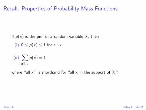
Recall: Properties of Probability Mass Functions
If p(x) is the pmf of a random variable X , then
(i) 0 ≤ p(x) ≤ 1 for all x
(ii)∑all x
p(x) = 1
where “all x” is shorthand for “all x in the support of X .”
Econ 103 Lecture 8 – Slide 2

Cumulative Distribution Function (CDF)This Def. is the same for continuous RVs.
The CDF gives the probability that a RV X does not exceed a
specified threshold x0, as a function of x0
F (x0) = P(X ≤ x0)
Important!
The threshold x0 is allowed to be any real number. In particular, it
doesn’t have to be in the support of X !
Econ 103 Lecture 8 – Slide 3

Discrete RVs: Sum the pmf to get the CDF
F (x0) =∑x≤x0
p(x)
Why?
The events {X = x} are mutually exclusive, so we sum to get the
probability of their union for all x ≤ x0:
F (x0) = P(X ≤ x0) = P
⋃x≤x0
{X = x}
=∑x≤x0
P(X = x) =∑x≤x0
p(x)
Econ 103 Lecture 8 – Slide 4

Probability Mass Function
p(x)
x0 1
1/2
p(0) = 1/2
p(1) = 1/2
Cumulative Dist. Function
F (x0)
x0
1
12
0 10
F (x0) =
0, x0 < 012 , 0 ≤ x0 < 1
1, x0 ≥ 1
Econ 103 Lecture 8 – Slide 5

Properties of CDFsThese are also true for continuous RVs.
1. limx0→∞ F (x0) = 1
2. limx0→−∞ F (x0) = 0
3. Non-decreasing: x0 < x1 ⇒ F (x0) ≤ F (x1)
4. Right-continuous (“open” versus “closed” on prev. slide)
Since F (x0) = P(X ≤ x0), we have 0 ≤ F (x0) ≤ 1 for all x0
Econ 103 Lecture 8 – Slide 6

Bernoulli Random Variable – Generalization of Coin Flip
Support Set
{0, 1} – 1 traditionally called “success,” 0 “failure”
Probability Mass Function
p(0) = 1− p
p(1) = p
Cumulative Distribution Function
F (x0) =
0, x0 < 0
1− p, 0 ≤ x0 < 1
1, x0 ≥ 1
Econ 103 Lecture 8 – Slide 7

http://fditraglia.shinyapps.io/binom cdf/Set the second slider to 1 and play around with the others.
Econ 103 Lecture 8 – Slide 8

Average Winnings Per Trial
If the realizations of the coin-flip RV were payoffs, how much would
you expect to win per play on average in a long sequence of plays?
X =
{$0,Tails
$1,Heads
Econ 103 Lecture 8 – Slide 9

Expected Value (aka Expectation)
The expected value of a discrete RV X is given by
E [X ] =∑all x
x · p(x)
In other words, the expected value of a discrete RV is the
probability-weighted average of its realizations.
Notation
We sometimes write µ as shorthand for E [X ].
Econ 103 Lecture 8 – Slide 10

Expected Value of Bernoulli RV
X =
{0,Failure: 1− p
1, Success: p
∑all x
x · p(x) = 0 · (1− p) + 1 · p = p
Econ 103 Lecture 8 – Slide 11

Your Turn to Calculate an Expected Value
Let X be a random variable with support set {1, 2, 3} where
p(1) = p(2) = 1/3. Calculate E [X ].
E [X ] =∑all x
x · p(x) = 1× 1/3 + 2× 1/3 + 3× 1/3 = 2
Econ 103 Lecture 8 – Slide 12

Random Variables and Parameters
Notation: X ∼ Bernoulli(p)
Means X is a Bernoulli RV with P(X = 1) = p and
P(X = 0) = 1− p. The tilde is read “distributes as.”
Parameter
Any constant that appears in the definition of a RV, here p.
Econ 103 Lecture 8 – Slide 13
Constants Versus Random Variables
This is a crucial distinction that students sometimes miss:
Random Variables
I Suppose X is a RV – the values it takes on are random
I A function g(X ) of a RV is itself a RV as we’ll learn today.
Constants
I E [X ] is a constant (you should convince yourself of this)
I Realizations x are constants. What is random is which
realization the RV takes on.
I Parameters are constants (e.g. p for Bernoulli RV)
I Sample size n is a constantEcon 103 Lecture 8 – Slide 14

The St. Petersburg Game
Econ 103 Lecture 8 – Slide 15

How Much Would You Pay?
How much would you be willing to pay for the right to play the
following game?
Imagine a fair coin. The coin is tossed once. If it falls
heads, you receive a prize of $2 and the game stops. If
not, it is tossed again. If it falls heads on the second
toss, you get $4 and the game stops. If not, it is tossed
again. If it falls heads on the third toss, you get $8 and
the game stops, and so on. The game stops after the
first head is thrown. If the first head is thrown on the x th
toss, the prize is $2x
Econ 103 Lecture 8 – Slide 16

X = Trial Number of First Head
x 2x p(x) 2x · p(x)1 2 1/2 1
2 4 1/4 1
3 8 1/8 1...
......
...
n 2n 1/2n 1...
......
...
E [Y ] =∑all x
2x · p(x) = 1 + 1 + 1 + . . . = ∞
Econ 103 Lecture 8 – Slide 17

Functions of Random Variables
are Themselves Random
Variables
Econ 103 Lecture 8 – Slide 18

Example: X ∼ Bernoulli(p), Y = (X + 1)2
Support Set for Y
{(0 + 1)2, (1 + 1)2} = {1, 4}
Probability Mass Function for Y
pY (y) =
1− p y = 1
p y = 4
0 otherwise
Expected Value of Y
∑y∈{1,4}
y × pY (y) = 1× (1− p) + 4× p = 1 + 3p
Econ 103 Lecture 8 – Slide 19

Example: X ∼ Bernoulli(p), Y = (X + 1)2
E [g(X )] = E [(X + 1)2]
∑y∈{1,4}
y × pY (y) = 1× (1− p) + 4× p = 1 + 3p
g(E [X ]) = (E [X ] + 1)2
(E [X ] + 1)2 = (p + 1)2 = 1 + 2p + p2
In general: 1 + 3p 6= 1 + 2p + p2!
Econ 103 Lecture 8 – Slide 20

E [g(X )] 6= g(E [X ])
(Expected value of Function 6= Function of Expected Value)
Econ 103 Lecture 8 – Slide 21

Expectation of a Function of a Discrete RV
Let X be a random variable and g be a function. Then:
E [g(X )] =∑all x
g(x)p(x)
This is how we proceeded in the St. Petersburg Game Example
Econ 103 Lecture 8 – Slide 22

Your Turn: Calculate E [X 2]
X has support {−1, 0, 1}, p(−1) = p(0) = p(1) = 1/3.
E [X 2] =∑all x
x2p(x) =∑
x∈{−1,0,1}
x2p(x)
= (−1)2 · (1/3) + (0)2 · (1/3) + (1)2 · (1/3)
= 1/3 + 1/3
= 2/3 ≈ 0.67
Econ 103 Lecture 8 – Slide 23

Linearity of ExpectationHolds for Continuous RVs as well, but proof is different.
Let X be a RV and a, b be constants. Then:
E [a+ bX ] = a+ bE [X ]
This is a Crucial Exception
In general E [g(X )] does not equal g(E [X ]). But in the special case
where g is a linear function, g(X ) = a+ bX , the two are equal.
Econ 103 Lecture 8 – Slide 24

Example: Linearity of Expectation
Let X ∼ Bernoulli(1/3) and define Y = 3X + 2
1. What is E [X ]? E [X ] = 0× 2/3 + 1× 1/3 = 1/3
2. What is E [Y ]? E [Y ] = E [3X + 2] = 3E [X ] + 2 = 3
Econ 103 Lecture 8 – Slide 25

Proof: Linearity of Expectation For Discrete RV
E [a+ bX ] =∑all x
(a+ bx)p(x)
=∑all x
p(x) · a+∑all x
p(x) · bx
= a∑all x
p(x) + b∑all x
x · p(x)
= a+ bE [X ]
Econ 103 Lecture 8 – Slide 26

Lecture #9 – Discrete RVs III
Variance and Standard Deviation of a Random Variable
Binomial Random Variable
Joint Probability Mass Function
Joint versus Marginal Probability Mass Function
Econ 103 Lecture 9 – Slide 1

Variance and Standard Deviation of a RVThe Defs are the same for continuous RVs, but the method of calculating will differ.
Variance (Var)
σ2 = Var(X ) = E[(X − µ)2
]= E
[(X − E [X ])2
]Standard Deviation (SD)
σ =√σ2 = SD(X )
Econ 103 Lecture 9 – Slide 2

Key Point
Variance and std. dev. are expectations of functions of a RV
It follows that:
1. Variance and SD are constants
2. To derive facts about them you can use the facts you know
about expected value
Econ 103 Lecture 9 – Slide 3

How To Calculate Variance for Discrete RV?Remember: it’s just a function of X !
Recall that µ = E [X ] =∑all x
xp(x)
Var(X ) = E[(X − µ)2
]=∑all x
(x − µ)2p(x)
Econ 103 Lecture 9 – Slide 4
Shortcut Formula For Variance
This is not the definition, it’s a shortcut for doing calculations:
Var(X ) = E[(X − µ)2
]= E [X 2]− (E [X ])2
We’ll prove this in an upcoming lecture.
Econ 103 Lecture 9 – Slide 5
Example: The Shortcut Formula
Let X ∼ Bernoulli(1/2). Calculate Var(X ).
E [X ] = 0× 1/2 + 1× 1/2 = 1/2
E [X 2] = 02 × 1/2 + 12 × 1/2 = 1/2
E [X 2]− (E [X ])2 = 1/2− (1/2)2 = 1/4
Econ 103 Lecture 9 – Slide 6

Variance of Bernoulli RV – via the Shortcut Formula
Step 1 – E [X ]
µ = E [X ] =∑
x∈{0,1}
p(x) · x = (1− p) · 0 + p · 1 = p
Step 2 – E [X 2]
E [X 2] =∑
x∈{0,1}
x2p(x) = 02(1− p) + 12p = p
Step 3 – Combine with Shortcut Formula
σ2 = Var [X ] = E [X 2]− (E [X ])2 = p − p2 = p(1− p)
Econ 103 Lecture 9 – Slide 7

Variance of a Linear Transformation
Var(a+ bX ) = E[{(a+ bX )− E (a+ bX )}2
]= E
[{(a+ bX )− (a+ bE [X ])}2
]= E
[(bX − bE [X ])2
]= E [b2(X − E [X ])2]
= b2E [(X − E [X ])2]
= b2Var(X ) = b2σ2
The key point here is that variance is defined in terms of
expectation and expectation is linear.
Econ 103 Lecture 9 – Slide 8

Variance and SD are NOT Linear
Var(a+ bX ) = b2σ2
SD(a+ bX ) = |b|σ
These should look familiar from the related results for sample
variance and std. dev. that you worked out on an earlier
problem set.
Econ 103 Lecture 9 – Slide 9

Binomial Random Variable
Let X = the sum of n independent Bernoulli trials, each with
probability of success p. Then we say that: X ∼ Binomial(n, p)
Parameters
p = probability of “success,” n = # of trials
Support
{0, 1, 2, . . . , n}
Probability Mass Function (pmf)
p(x) =
(n
x
)px(1− p)n−x
Econ 103 Lecture 9 – Slide 10

http://fditraglia.shinyapps.io/binom cdf/Try playing around with all three sliders. If you set the second to 1 you get a Bernoulli.
Econ 103 Lecture 9 – Slide 11
http://fditraglia.github.com/Econ103Public/Rtutorials/Bernoulli Binomial.html
Source Code on my Github Page
Don’t forget this!
Binomial RV counts up the total number of successes (ones) in n
indep. Bernoulli trials, each with prob. of success p.Econ 103 Lecture 9 – Slide 12

Where does the Binomial pmf come from?
Question
Suppose we flip a fair coin 3 times. What is the probability that we
get exactly 2 heads?
Answer
Three basic outcomes make up this event: {HHT ,HTH,THH},each has probability 1/8 = 1/2× 1/2× 1/2. Basic outcomes are
mutually exclusive, so sum to get 3/8 = 0.375
Econ 103 Lecture 9 – Slide 13

Where does the Binomial pmf come from?
Question
Suppose we flip an unfair coin 3 times, where the probability of
heads is 1/3. What is the probability that we get exactly 2 heads?
Answer
No longer true that all basic outcomes are equally likely, but those
with exactly two heads still are
P(HHT ) = (1/3)2(1− 1/3) = 2/27
P(THH) = 2/27
P(HTH) = 2/27
Summing gives 2/9 ≈ 0.22
Econ 103 Lecture 9 – Slide 14

Where does the Binomial pmf come from?Starting to see a pattern?
Suppose we flip an unfair coin 4 times, where the probability of
heads is 1/3. What is the probability that we get exactly 2 heads?
HHTT TTHH
HTHT THTH
HTTH THHT
Six equally likely, mutually exclusive
basic outcomes make up this event:(4
2
)(1/3)2(2/3)2
Econ 103 Lecture 9 – Slide 15
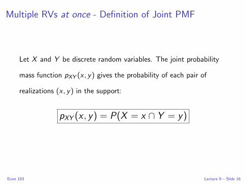
Multiple RVs at once - Definition of Joint PMF
Let X and Y be discrete random variables. The joint probability
mass function pXY (x , y) gives the probability of each pair of
realizations (x , y) in the support:
pXY (x , y) = P(X = x ∩ Y = y)
Econ 103 Lecture 9 – Slide 16

Example: Joint PMF in Tabular Form
Y
1 2 3
X
0 1/8 0 0
1 0 1/4 1/8
2 0 1/4 1/8
3 1/8 0 0
Econ 103 Lecture 9 – Slide 17

Plot of Joint PMF
0 1 2 30.10
0.15
0.20
0.25
1
2
3
x
y
p(x,
y)
Econ 103 Lecture 9 – Slide 18

What is pXY (1, 2)?
Y
1 2 3
X
0 1/8 0 0
1 0 1/4 1/8
2 0 1/4 1/8
3 1/8 0 0
pXY (1, 2) = P(X = 1 ∩ Y = 2) = 1/4
pXY (2, 1) = P(X = 2 ∩ Y = 1) = 0
Econ 103 Lecture 9 – Slide 19
Properties of Joint PMF
1. 0 ≤ pXY (x , y) ≤ 1 for any pair (x , y)
2. The sum of pXY (x , y) over all pairs (x , y) in the support is 1:
∑x
∑y
p(x , y) = 1
Econ 103 Lecture 9 – Slide 20

Joint versus Marginal PMFs
Joint PMF
pXY (x , y) = P(X = x ∩ Y = y)
Marginal PMFs
pX (x) = P(X = x)
pY (y) = P(Y = y)
You can’t calculate a joint pmf from marginals alone but you can
calculate marginals from the joint!
Econ 103 Lecture 9 – Slide 21

Marginals from Joint
pX (x) =∑all y
pXY (x , y)
pY (y) =∑all x
pXY (x , y)
Why?
pY (y) = P(Y = y) = P
⋃all x
{X = x ∩ Y = y}
=
∑all x
P(X = x ∩ Y = y) =∑all x
pXY (x , y)
Econ 103 Lecture 9 – Slide 22

To get the marginals sum “into the margins” of the table.
Y
1 2 3
X
0 1/8 0 0 1/8
1 0 1/4 1/8 3/8
2 0 1/4 1/8 3/8
3 1/8 0 0 1/8
1
pX (0) = 1/8 + 0 + 0 = 1/8
pX (1) = 0 + 1/4 + 1/8 = 3/8
pX (2) = 0 + 1/4 + 1/8 = 3/8
pX (3) = 1/8 + 0 + 0 = 1/8Econ 103 Lecture 9 – Slide 23
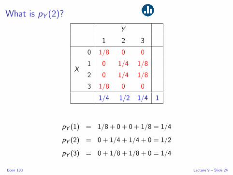
What is pY (2)?
Y
1 2 3
X
0 1/8 0 0
1 0 1/4 1/8
2 0 1/4 1/8
3 1/8 0 0
1/4 1/2 1/4 1
pY (1) = 1/8 + 0 + 0 + 1/8 = 1/4
pY (2) = 0 + 1/4 + 1/4 + 0 = 1/2
pY (3) = 0 + 1/8 + 1/8 + 0 = 1/4
Econ 103 Lecture 9 – Slide 24

Lecture #10 – Discrete RVs IV
Conditional Probability Mass Function & Independence
Conditional Expectation & The Law of Iterated Expectations
Expectation of a Function of Two Discrete RVs, Covariance
Linearity of Expectation Reprise, Properties of Binomial RV
Econ 103 Lecture 10 – Slide 1
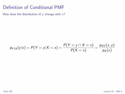
Definition of Conditional PMFHow does the distribution of y change with x?
pY |X (y |x) = P(Y = y |X = x) =P(Y = y ∩ X = x)
P(X = x)=
pXY (x , y)
pX (x)
Econ 103 Lecture 10 – Slide 2

Conditional PMF of Y given X = 2
Y
1 2 3
X
0 1/8 0 0 1/8
1 0 1/4 1/8 3/8
2 0 1/4 1/8 3/8
3 1/8 0 0 1/8
pY |X (1|2) =pXY (2, 1)
pX (2)=
0
3/8= 0
pY |X (2|2) =pXY (2, 2)
pX (2)=
1/4
3/8= 2/3
pY |X (3|2) =pXY (2, 3)
pX (2)=
1/8
3/8= 1/3
Econ 103 Lecture 10 – Slide 3
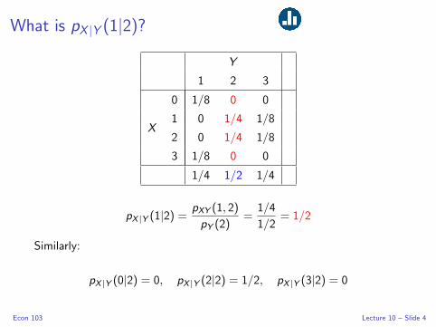
What is pX |Y (1|2)?
Y
1 2 3
X
0 1/8 0 0
1 0 1/4 1/8
2 0 1/4 1/8
3 1/8 0 0
1/4 1/2 1/4
pX |Y (1|2) =pXY (1, 2)
pY (2)=
1/4
1/2= 1/2
Similarly:
pX |Y (0|2) = 0, pX |Y (2|2) = 1/2, pX |Y (3|2) = 0
Econ 103 Lecture 10 – Slide 4

Independent RVs: Joint Equals Product of Marginals
Definition
Two discrete RVs are independent if and only if
pXY (x , y) = pX (x)pY (y)
for all pairs (x , y) in the support.
Equivalent Definition
pY |X (y |x) = pY (y) and pX |Y (x |y) = pX (x)
for all pairs (x , y) in the support.
Econ 103 Lecture 10 – Slide 5
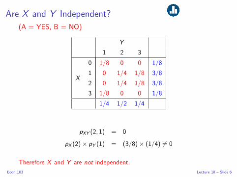
Are X and Y Independent?
(A = YES, B = NO)
Y
1 2 3
X
0 1/8 0 0 1/8
1 0 1/4 1/8 3/8
2 0 1/4 1/8 3/8
3 1/8 0 0 1/8
1/4 1/2 1/4
pXY (2, 1) = 0
pX (2)× pY (1) = (3/8)× (1/4) 6= 0
Therefore X and Y are not independent.
Econ 103 Lecture 10 – Slide 6

Conditional Expectation
Intuition
E [Y |X ] = “best guess” of realization that Y after observing
realization of X .
E [Y |X ] is a Random Variable
While E [Y ] is a constant, E [Y |X ] is a function of X , hence a
Random Variable.
E [Y |X = x ] is a Constant
The constant E [Y |X = x ] is the “guess” of Y if we see X = x .
Calculating E [Y |X = x ]
Take the mean of the conditional pmf of Y given X = x .
Econ 103 Lecture 10 – Slide 7

Conditional Expectation: E [Y |X = 2]
Y
1 2 3
X
0 1/8 0 0 1/8
1 0 1/4 1/8 3/8
2 0 1/4 1/8 3/8
3 1/8 0 0 1/8
1/4 1/2 1/4
We showed above that the conditional pmf of Y |X = 2 is:
pY |X (1|2) = 0 pY |X (2|2) = 2/3 pY |X (3|2) = 1/3
Hence
E [Y |X = 2] = 2× 2/3 + 3× 1/3 = 7/3
Econ 103 Lecture 10 – Slide 8

Conditional Expectation: E [Y |X = 0]
Y
1 2 3
X
0 1/8 0 0 1/8
1 0 1/4 1/8 3/8
2 0 1/4 1/8 3/8
3 1/8 0 0 1/8
1/4 1/2 1/4
The conditional pmf of Y |X = 0 is
pY |X (1|0) = 1 pY |X (2|0) = 0 pY |X (3|0) = 0
Hence E [Y |X = 0] = 1
Econ 103 Lecture 10 – Slide 9

Calculate E [Y |X = 3]
Y
1 2 3
X
0 1/8 0 0 1/8
1 0 1/4 1/8 3/8
2 0 1/4 1/8 3/8
3 1/8 0 0 1/8
1/4 1/2 1/4
The conditional pmf of Y |X = 3 is
pY |X (1|3) = 1 pY |X (2|3) = 0 pY |X (3|3) = 0
Hence E [Y |X = 3] = 1
Econ 103 Lecture 10 – Slide 10
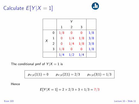
Calculate E [Y |X = 1]
Y
1 2 3
X
0 1/8 0 0 1/8
1 0 1/4 1/8 3/8
2 0 1/4 1/8 3/8
3 1/8 0 0 1/8
1/4 1/2 1/4
The conditional pmf of Y |X = 1 is
pY |X (1|1) = 0 pY |X (2|1) = 2/3 pY |X (3|1) = 1/3
Hence
E [Y |X = 1] = 2× 2/3 + 3× 1/3 = 7/3
Econ 103 Lecture 10 – Slide 11
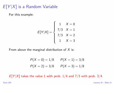
E [Y |X ] is a Random Variable
For this example:
E [Y |X ] =
1 X = 0
7/3 X = 1
7/3 X = 2
1 X = 3
From above the marginal distribution of X is:
P(X = 0) = 1/8 P(X = 1) = 3/8
P(X = 2) = 3/8 P(X = 3) = 1/8
E [Y |X ] takes the value 1 with prob. 1/4 and 7/3 with prob. 3/4.
Econ 103 Lecture 10 – Slide 12

The Law of Iterated ExpectationsE [Y |X ] is an RV so what is its expectation?
For any RVs X and Y
E [E [Y |X ]] = E [Y ]
Option proof HERE . (Helpful for Econ 104. . . )
Econ 103 Lecture 10 – Slide 13

Law of Iterated Expectations for Our Example
Marginal pmf of Y
P(Y = 1) = 1/4
P(Y = 2) = 1/2
P(Y = 3) = 1/4
E [Y ] = 1× 1/4 + 2× 1/2 + 3× 1/4
= 2
E [Y |X ]
E [Y |X ] =
{1 w/ prob. 1/4
7/3 w/ prob. 3/4
E [E [Y |X ]] = 1× 1/4 + 7/3× 3/4
= 2
Econ 103 Lecture 10 – Slide 14
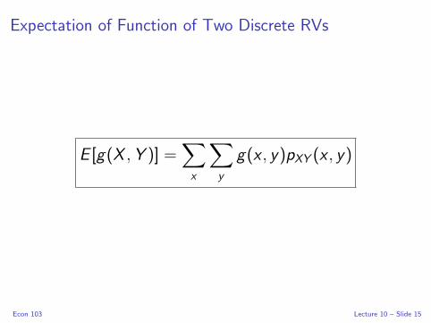
Expectation of Function of Two Discrete RVs
E [g(X ,Y )] =∑x
∑y
g(x , y)pXY (x , y)
Econ 103 Lecture 10 – Slide 15

Some Extremely Important ExamplesSame For Continuous Random Variables
Let µX = E [X ], µY = E [Y ]
Covariance
σXY = Cov(X ,Y ) = E [(X − µX )(Y − µY )]
Correlation
ρXY = Corr(X ,Y ) =σXYσXσY
Econ 103 Lecture 10 – Slide 16
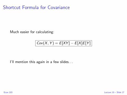
Shortcut Formula for Covariance
Much easier for calculating:
Cov(X ,Y ) = E [XY ]− E [X ]E [Y ]
I’ll mention this again in a few slides. . .
Econ 103 Lecture 10 – Slide 17

Calculating Cov(X ,Y )
Y
1 2 3
X
0 1/8 0 0 1/8
1 0 1/4 1/8 3/8
2 0 1/4 1/8 3/8
3 1/8 0 0 1/8
1/4 1/2 1/4
E [X ] = 3/8 + 2× 3/8 + 3× 1/8 = 3/2
E [Y ] = 1/4 + 2× 1/2 + 3× 1/4 = 2
E [XY ] = 1/4× (2 + 4) + 1/8× (3 + 6 + 3)
= 3
Cov(X ,Y ) = E [XY ]− E [X ]E [Y ]
= 3− 3/2× 2 = 0
Corr(X ,Y ) = Cov(X ,Y )/ [SD(X )SD(Y )] = 0
Econ 103 Lecture 10 – Slide 18
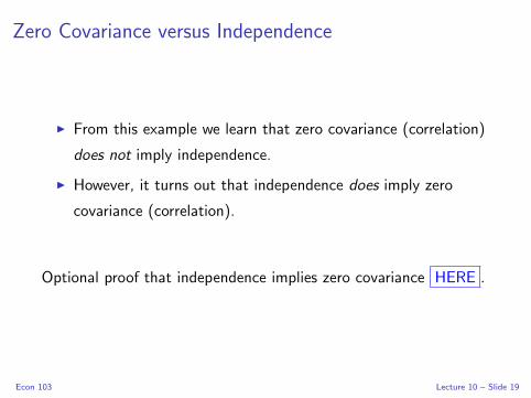
Zero Covariance versus Independence
I From this example we learn that zero covariance (correlation)
does not imply independence.
I However, it turns out that independence does imply zero
covariance (correlation).
Optional proof that independence implies zero covariance HERE .
Econ 103 Lecture 10 – Slide 19

Linearity of Expectation, AgainHolds for Continuous RVs as well, but different proof.
In general, E [g(X ,Y )] 6= g(E [X ],E [Y ]). The key exception is
when g is a linear function:
E [aX + bY + c] = aE [X ] + bE [Y ] + c
where X ,Y are random variables and a, b, c are constants.
Optional proof HERE .
Econ 103 Lecture 10 – Slide 20

Application: Shortcut Formula for Variance
By the Linearity of Expectation,
Var(X ) = E [(X − µ)2] = E [X 2 − 2µX + µ2]
= E [X 2]− 2µE [X ] + µ2
= E [X 2]− 2µ2 + µ2
= E [X 2]− µ2
We saw in a previous lecture that it’s typically much easier to
calculate variances using the shortcut formula.
Econ 103 Lecture 10 – Slide 21

Another Application: Shortcut Formula for Covariance
Similar to Shortcut for Variance: in fact Var(X ) = Cov(X ,X )
Cov(X ,Y ) = E [(X − µX )(Y − µY )]
= E [XY − µXY − µYX + µXµY ]...
= E [XY ]− E [X ]E [Y ]
You’ll fill in the details for homework...
Econ 103 Lecture 10 – Slide 22
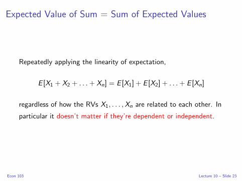
Expected Value of Sum = Sum of Expected Values
Repeatedly applying the linearity of expectation,
E [X1 + X2 + . . .+ Xn] = E [X1] + E [X2] + . . .+ E [Xn]
regardless of how the RVs X1, . . . ,Xn are related to each other. In
particular it doesn’t matter if they’re dependent or independent.
Econ 103 Lecture 10 – Slide 23

Independent and Identically Distributed (iid) RVs
Example
X1,X2, . . .Xn ∼ iid Bernoulli(p)
Independent
Realization of one of the RVs gives no information about the
others.
Identically Distributed
Each Xi is the same kind of RV, with the same values for any
parameters. (Hence same pmf, cdf, mean, variance, etc.)
Econ 103 Lecture 10 – Slide 24

Recall: Binomial(n, p) Random Variable
Definition
Sum of n independent Bernoulli RVs, each with probability of
“success,” i.e. 1, equal to p
Using Our New Notation
Let X1,X2, . . . ,Xn ∼ iid Bernoulli(p), Y = X1 + X2 + . . .+ Xn.
Then Y ∼ Binomial(n, p).
Econ 103 Lecture 10 – Slide 25

Expected Value of Binomial RV
Use the fact that a Binomial(n, p) RV is defined as the sum of n iid
Bernoulli(p) Random Variables and the Linearity of Expectation:
E [Y ] = E [X1 + X2 + . . .+ Xn] = E [X1] + E [X2] + . . .+ E [Xn]
= p + p + . . .+ p
= np
Econ 103 Lecture 10 – Slide 26
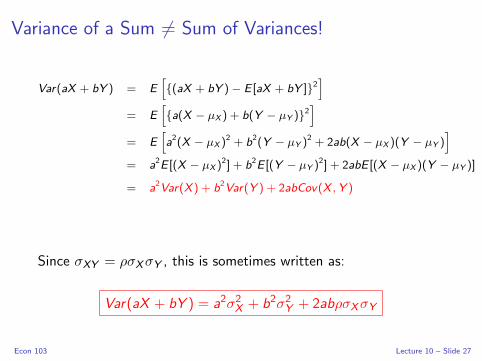
Variance of a Sum 6= Sum of Variances!
Var(aX + bY ) = E[{(aX + bY )− E [aX + bY ]}2
]= E
[{a(X − µX ) + b(Y − µY )}2
]= E
[a2(X − µX )
2 + b2(Y − µY )2 + 2ab(X − µX )(Y − µY )
]= a2E [(X − µX )
2] + b2E [(Y − µY )2] + 2abE [(X − µX )(Y − µY )]
= a2Var(X ) + b2Var(Y ) + 2abCov(X ,Y )
Since σXY = ρσXσY , this is sometimes written as:
Var(aX + bY ) = a2σ2X + b2σ2
Y + 2abρσXσY
Econ 103 Lecture 10 – Slide 27
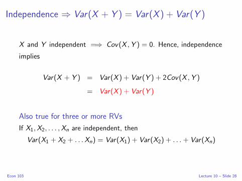
Independence ⇒ Var(X + Y ) = Var(X ) + Var(Y )
X and Y independent =⇒ Cov(X ,Y ) = 0. Hence, independence
implies
Var(X + Y ) = Var(X ) + Var(Y ) + 2Cov(X ,Y )
= Var(X ) + Var(Y )
Also true for three or more RVs
If X1,X2, . . . ,Xn are independent, then
Var(X1 + X2 + . . .Xn) = Var(X1) + Var(X2) + . . .+ Var(Xn)
Econ 103 Lecture 10 – Slide 28

Crucial Distinction
Expected Value
Always true that
E [X1 + X2 + . . .+ Xn] = E [X1] + E [X2] + . . .+ E [Xn]
Variance
Not true in general that
Var [X1 + X2 + . . .+ Xn] = Var [X1] + Var [X2] + . . .+ Var [Xn]
except in the special case where X1, . . .Xn are independent (or at
least uncorrelated).
Econ 103 Lecture 10 – Slide 29

Variance of Binomial Random Variable
Definition from Sequence of Bernoulli Trials
If X1,X2, . . . ,Xn ∼ iid Bernoulli(p) then
Y = X1 + X2 + . . .+ Xn ∼ Binomial(n, p)
Using Independence
Var [Y ] = Var [X1 + X2 + . . .+ Xn]
= Var [X1] + Var [X2] + . . .+ Var [Xn]
= p(1− p) + p(1− p) + . . .+ p(1− p)
= np(1− p)
Econ 103 Lecture 10 – Slide 30

Lecture #11 – Continuous RVs I
Introduction: Probability as Area
Probability Density Function (PDF)
Relating the PDF to the CDF
Calculating the Probability of an Interval
Calculating Expected Value for Continuous RVs
Econ 103 Lecture 11 – Slide 1

Continuous RVs – What Changes?
1. Probability Density Functions replace Probability Mass
Functions (aka Probability Distributions)
2. Integrals Replace Sums
Everything Else is Essentially Unchanged!
Econ 103 Lecture 11 – Slide 2

What is the probability of “Yellow?”
Econ 103 Lecture 11 – Slide 3

From Twister to Density – Probability as Area
0.0 0.2 0.4 0.6 0.8 1.0
0.0
0.2
0.4
0.6
0.8
1.0
x
f(x)
Econ 103 Lecture 11 – Slide 4

Continuous Random Variables
For continuous RVs, probability is a matter of finding the area of
intervals. Individual points have zero probability.
Econ 103 Lecture 11 – Slide 5

Probability Density Function (PDF)
For a continuous random variable X ,
P(a ≤ X ≤ b) =
∫ b
af (x) dx
where f (x) is the probability density function for X .
Extremely Important
For any realization x , P(X = x) = 0 6= f (x)!
Econ 103 Lecture 11 – Slide 6

Properties of PDFs
1.∫∞−∞ f (x) dx = 1
2. f (x) ≥ 0 for all x
3. f (x) is not a probability and can be greater than one!
4. P(X ≤ x0) = F (x0) =∫ x0−∞ f (x) dx
Econ 103 Lecture 11 – Slide 7

Simplest Possible Continuous RV: Uniform(0, 1)You’ll look at a generalization, Uniform(a, b) for homework.
X ∼ Uniform(0, 1)
A Uniform(0,1) RV is equally likely to take on any value in the
range [0, 1] and never takes on a value outside this range.
Uniform PDF
f (x) = 1 for 0 ≤ x ≤ 1, zero elsewhere.
Econ 103 Lecture 11 – Slide 8

Uniform(0, 1) PDF
0.0 0.2 0.4 0.6 0.8 1.0
0.0
0.2
0.4
0.6
0.8
1.0
x
f(x)
Econ 103 Lecture 11 – Slide 9

Check that Uniform pdf Integrates to 1
0.0 0.2 0.4 0.6 0.8 1.0
0.0
0.2
0.4
0.6
0.8
1.0
x
f(x)
∫ ∞
−∞f (x) dx =
∫ 1
01 dx = x |10 = 1− 0 = 1
Econ 103 Lecture 11 – Slide 10

What is the area of the shaded region?
0.0 0.2 0.4 0.6 0.8 1.0
0.0
0.2
0.4
0.6
0.8
1.0
x
f(x)
Econ 103 Lecture 11 – Slide 11
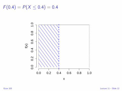
F (0.4) = P(X ≤ 0.4) = 0.4
0.0 0.2 0.4 0.6 0.8 1.0
0.0
0.2
0.4
0.6
0.8
1.0
x
f(x)
Econ 103 Lecture 11 – Slide 12

Relationship between PDF and CDF
Integrate pdf → CDF
F (x0) = P(X ≤ x0) =
∫ x0
−∞f (x) dx
Differentiate CDF → pdf
f (x) =d
dxF (x)
This is just the First Fundamental Theorem of Calculus.
Econ 103 Lecture 11 – Slide 13

Example: Uniform(0, 1) RV
Integrate the pdf, f (x) = 1, to get the CDF
F (x0) =
∫ x0
−∞f (x) dx =
∫ x0
01 dx = x |x00 = x0 − 0 = x0
F (x0) =
0, x0 < 0
x0, 0 ≤ x0 ≤ 1
1, x0 > 1
Econ 103 Lecture 11 – Slide 14

Uniform(0, 1) CDF
0.0 0.2 0.4 0.6 0.8 1.0
0.0
0.2
0.4
0.6
0.8
1.0
x
F(x
)
Econ 103 Lecture 11 – Slide 15
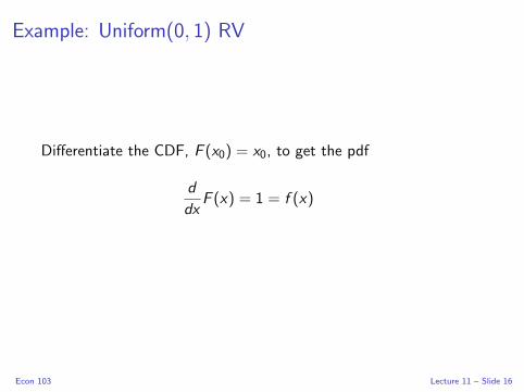
Example: Uniform(0, 1) RV
Differentiate the CDF, F (x0) = x0, to get the pdf
d
dxF (x) = 1 = f (x)
Econ 103 Lecture 11 – Slide 16

What is P(0.4 ≤ X ≤ 0.8) if X ∼ Uniform(0, 1)?
0.0 0.2 0.4 0.6 0.8 1.0
0.0
0.2
0.4
0.6
0.8
1.0
x
f(x)
Econ 103 Lecture 11 – Slide 17

F (0.8) = P(X ≤ 0.8)
0.0 0.2 0.4 0.6 0.8 1.0
0.0
0.2
0.4
0.6
0.8
1.0
x
f(x)
Econ 103 Lecture 11 – Slide 18

F (0.8)− F (0.4) = ?
0.0 0.2 0.4 0.6 0.8 1.0
0.0
0.2
0.4
0.6
0.8
1.0
x
f(x)
Econ 103 Lecture 11 – Slide 19
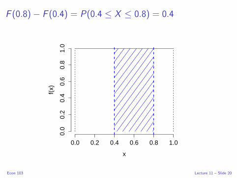
F (0.8)− F (0.4) = P(0.4 ≤ X ≤ 0.8) = 0.4
0.0 0.2 0.4 0.6 0.8 1.0
0.0
0.2
0.4
0.6
0.8
1.0
x
f(x)
Econ 103 Lecture 11 – Slide 20

Key Idea: Probability of Interval for Continuous RV
P(a ≤ X ≤ b) =
∫ b
af (x) dx = F (b)− F (a)
This is just the Second Fundamental Theorem of Calculus.
Econ 103 Lecture 11 – Slide 21

Expected Value for Continuous RVs
∫ ∞
−∞xf (x) dx
Remember: Integrals Replace Sums!
Econ 103 Lecture 11 – Slide 22
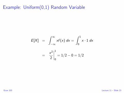
Example: Uniform(0,1) Random Variable
E [X ] =
∫ ∞
−∞xf (x) dx =
∫ 1
0x · 1 dx
=x2
2
∣∣∣∣10
= 1/2− 0 = 1/2
Econ 103 Lecture 11 – Slide 23

Expected Value of a Function of a Continuous RV
E [g(X )] =
∫ ∞
−∞g(x)f (x) dx
Econ 103 Lecture 11 – Slide 24

Example: Uniform(0,1) Random Variable
E [X 2] =
∫ ∞
−∞x2f (x) dx =
∫ 1
0x2 · 1 dx
=x3
3
∣∣∣∣10
= 1/3
Econ 103 Lecture 11 – Slide 25

What about all those rules for expected value?
I The only difference between expectation for continuous versus
discrete is how we do the calculation.
I Sum for discrete; integral for continuous.
I All properties of expected value continue to hold!
I Includes linearity, shortcut for variance, etc.
Econ 103 Lecture 11 – Slide 26
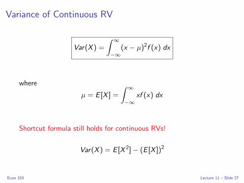
Variance of Continuous RV
Var(X ) =
∫ ∞
−∞(x − µ)2f (x) dx
where
µ = E [X ] =
∫ ∞
−∞xf (x) dx
Shortcut formula still holds for continuous RVs!
Var(X ) = E [X 2]− (E [X ])2
Econ 103 Lecture 11 – Slide 27

Example: Uniform(0, 1) RV
Var(X ) = E[(X − E [X ])2
]= E [X 2]− (E [X ])2
= 1/3− (1/2)2
= 1/12
≈ 0.083
Econ 103 Lecture 11 – Slide 28

So where does that leave us?
What We’ve Accomplished
We’ve covered all the basic properties of RVs on this Handout .
Where are we headed next?
Next up is the most important RV of all: the normal RV. After
that it’s time to do some statistics!
How should you be studying?
If you master the material on RVs (both continuous and discrete)
and in particular the normal RV the rest of the semester will seem
easy. If you don’t, you’re in for a rough time. . .
Econ 103 Lecture 11 – Slide 29

Lecture #12 – Continuous RVs II: The Normal RV
The Standard Normal RV
Linear Combinations and the N(µ, σ2) RV
Where does the Empirical Rule come from?
From N(0, 1) to N(µ, σ2) and Back Again
Percentiles/Quantiles for Continuous RVs
Econ 103 Lecture 12 – Slide 1

Available on Etsy, Made using R!
Figure: Standard Normal RV (PDF)
Econ 103 Lecture 12 – Slide 2

Standard Normal Random Variable: N(0, 1)
−4 −2 0 2 4
0.0
0.1
0.2
0.3
0.4
x
f(x)
−4 −2 0 2 4
0.0
0.2
0.4
0.6
0.8
1.0
x
F(x
)
Figure: Standard Normal PDF (left) and CDF (Right)
I Notation: X ∼ N(0, 1)
I Symmetric, Bell-shaped, E [X ] = 0, Var [X ] = 1
I Support Set = (−∞,∞)
Econ 103 Lecture 12 – Slide 3

https://fditraglia.shinyapps.io/normal cdf/
Econ 103 Lecture 12 – Slide 4

Standard Normal Random Variable: N(0, 1)
−4 −2 0 2 4
0.0
0.1
0.2
0.3
0.4
x
f(x)
−4 −2 0 2 4
0.0
0.2
0.4
0.6
0.8
1.0
x
F(x
)I There is no closed-form expression for the N(0, 1) CDF.
I For Econ 103, don’t need to know formula for N(0, 1) PDF.
I You do need to know the R commands. . .
Econ 103 Lecture 12 – Slide 5

R Commands for the Standard Normal RV
dnorm – Standard Normal PDF
I Mnemonic: d = density, norm = normal
I Example: dnorm(0) gives height of N(0, 1) PDF at zero.
pnorm – Standard Normal CDF
I Mnemonic: p = probability, norm = normal
I Example: pnorm(1) = P(X ≤ 1) if X ∼ N(0, 1).
rnorm – Simulate Standard Normal Draws
I Mnemonic: r = random, norm = normal.
I Example: rnorm(10) makes ten iid N(0, 1) draws.
Econ 103 Lecture 12 – Slide 6

Φ(x0) Denotes the N(0, 1) CDF
You will sometimes encounter the notation Φ(x0). It means the
same thing as pnorm(x0) but it’s not an R command.
Econ 103 Lecture 12 – Slide 7
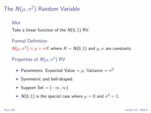
The N(µ, σ2) Random Variable
Idea
Take a linear function of the N(0, 1) RV.
Formal Definition
N(µ, σ2) ≡ µ+ σX where X ∼ N(0, 1) and µ, σ are constants.
Properties of N(µ, σ2) RV
I Parameters: Expected Value = µ, Variance = σ2
I Symmetric and bell-shaped.
I Support Set = (−∞,∞)
I N(0, 1) is the special case where µ = 0 and σ2 = 1.
Econ 103 Lecture 12 – Slide 8

Expected Value: µ shifts PDFall of these have σ = 1
−4 −2 0 2 4
0.0
0.1
0.2
0.3
0.4
x
f(x)
µ = −1µ = 0µ = 1
Figure: Blue µ = −1, Black µ = 0, Red µ = 1Econ 103 Lecture 12 – Slide 9

Standard Deviation: σ scales PDFall of these have µ = 0
−4 −2 0 2 4
0.0
0.2
0.4
0.6
0.8
x
f(x)
σ = 2σ = 1σ = 1/2
Figure: Blue σ2 = 4, Black σ2 = 1, Red σ2 = 1/4Econ 103 Lecture 12 – Slide 10

Linear Function of Normal RV is a Normal RV
Suppose that X ∼ N(µ, σ2). Then if a and b constants,
a+ bX ∼ N(a+ bµ, b2σ2)
Important
I For any RV X , E [a+ bX ] = a+ bE [X ] and
Var(a+ bX ) = b2Var(X ).
I Key point: linear transformation of normal is still normal!
I Linear transformation of Binomial is not Binomial!
Econ 103 Lecture 12 – Slide 11

Example
Suppose X ∼ N(µ, σ2) and let Z = (X − µ)/σ. What is the
distribution of Z?
(a) N(µ, σ2)
(b) N(µ, σ)
(c) N(0, σ2)
(d) N(0, σ)
(e) N(0, 1)
Econ 103 Lecture 12 – Slide 12

Linear Combinations of Multiple Independent Normals
Let X ∼ N(µx , σ2x) independent of Y ∼ N(µy , σ
2y ). Then if a, b, c
are constants:
aX + bY + c ∼ N(aµx + bµy + c , a2σ2x + b2σ2
y )
Important
I Result assumes independence
I Particular to Normal RV
I Extends to more than two Normal RVs
Econ 103 Lecture 12 – Slide 13

Suppose X1,X2,∼ iid N(µ, σ2)
Let X = (X1 + X2)/2. What is the distribution of X?
(a) N(µ, σ2/2)
(b) N(0, 1)
(c) N(µ, σ2)
(d) N(µ, 2σ2)
(e) N(2µ, 2σ2)
Econ 103 Lecture 12 – Slide 14

Where does the Empirical Rule come from?
Empirical Rule
Approximately 68% of observations within µ± σ
Approximately 95% of observations within µ± 2σ
Nearly all observations within µ± 3σ
Econ 103 Lecture 12 – Slide 15

pnorm(1)≈ 0.84
−4 −2 0 2 4
0.0
0.1
0.2
0.3
0.4
x
f(x)
Econ 103 Lecture 12 – Slide 16

pnorm(1) - pnorm(-1)≈ 0.84− 0.16
−4 −2 0 2 4
0.0
0.1
0.2
0.3
0.4
x
f(x)
Econ 103 Lecture 12 – Slide 17

pnorm(1) - pnorm(-1)≈ 0.68
−4 −2 0 2 4
0.0
0.1
0.2
0.3
0.4
x
f(x)
Econ 103 Lecture 12 – Slide 18

Middle 68% of N(0, 1) ⇒ approx. (−1, 1)
−4 −2 0 2 4
0.0
0.1
0.2
0.3
0.4
x
f(x)
Econ 103 Lecture 12 – Slide 19

Suppose X ∼ N(0, 1)
P(−1 ≤ X ≤ 1) = pnorm(1) - pnorm(-1)
≈ 0.683
P(−2 ≤ X ≤ 2) = pnorm(2) - pnorm(-2)
≈ 0.954
P(−3 ≤ X ≤ 3) = pnorm(3) - pnorm(-3)
≈ 0.997
Econ 103 Lecture 12 – Slide 20

What if X ∼ N(µ, σ2)?
P(X ≤ a) = P(X − µ ≤ a− µ)
= P
(X − µ
σ≤ a− µ
σ
)
= P
(Z ≤ a− µ
σ
)Where Z is a standard normal random variable, i.e. N(0, 1).
Econ 103 Lecture 12 – Slide 21

Which of these equals P (Z ≤ (a− µ)/σ) if Z ∼ N(0, 1)?
(a) pnorm(a)
(b) 1− pnorm(a)
(c) pnorm(a)/σ − µ
(d) pnorm(a−µ
σ
)(e) None of the above.
Econ 103 Lecture 12 – Slide 22

Probability Above a Threshold: X ∼ N(µ, σ2)
P(X ≥ b) = 1− P(X ≤ b) = 1− P
(X − µ
σ≤ b − µ
σ
)
= 1− P
(Z ≤ b − µ
σ
)= 1− pnorm((b − µ)/σ)
Where Z is a standard normal random variable.
Econ 103 Lecture 12 – Slide 23

Probability of an Interval: X ∼ N(µ, σ2)
P(a ≤ X ≤ b) = P
(a− µ
σ≤ X − µ
σ≤ b − µ
σ
)
= P
(a− µ
σ≤ Z ≤ b − µ
σ
)
= pnorm((b − µ)/σ)− pnorm((a− µ)/σ)
Where Z is a standard normal random variable.
Econ 103 Lecture 12 – Slide 24
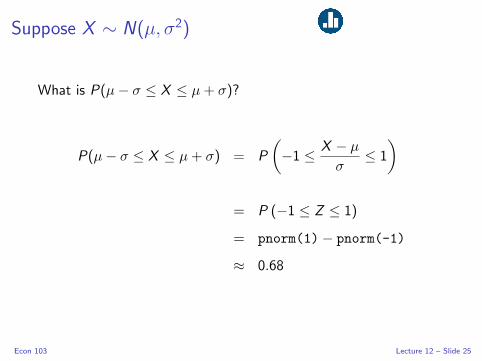
Suppose X ∼ N(µ, σ2)
What is P(µ− σ ≤ X ≤ µ+ σ)?
P(µ− σ ≤ X ≤ µ+ σ) = P
(−1 ≤ X − µ
σ≤ 1
)
= P (−1 ≤ Z ≤ 1)
= pnorm(1)− pnorm(-1)
≈ 0.68
Econ 103 Lecture 12 – Slide 25
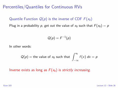
Percentiles/Quantiles for Continuous RVs
Quantile Function Q(p) is the inverse of CDF F (x0)
Plug in a probability p, get out the value of x0 such that F (x0) = p
Q(p) = F−1(p)
In other words:
Q(p) = the value of x0 such that
∫ x0
−∞f (x) dx = p
Inverse exists as long as F (x0) is strictly increasing.
Econ 103 Lecture 12 – Slide 26

Example: Median
The median of a continuous random variable is Q(0.5), i.e. the
value of x0 such that ∫ x0
−∞f (x) dx = 1/2
Econ 103 Lecture 12 – Slide 27

What is the median of a standard normal RV?
By symmetry, Q(0.5) = 0. R command: qnorm()
−4 −2 0 2 4
0.0
0.1
0.2
0.3
0.4
x
f(x)
Econ 103 Lecture 12 – Slide 28

90th Percentile of a Standard Normal
qnorm(0.9)≈ 1.28
−4 −2 0 2 4
0.0
0.1
0.2
0.3
0.4
x
f(x)
Econ 103 Lecture 12 – Slide 29

Using Quantile Function to find Symmetric Intervals
Suppose X is a standard normal RV. What is the value of c such
that P(−c ≤ X ≤ c) = 0.5?
−4 −2 0 2 4
0.0
0.1
0.2
0.3
0.4
x
f(x)
Econ 103 Lecture 12 – Slide 30

qnorm(0.75)≈ 0.67
Suppose X is a standard normal RV. What is the value of c such
that P(−c ≤ X ≤ c) = 0.5?
−4 −2 0 2 4
0.0
0.1
0.2
0.3
0.4
x
f(x)
Econ 103 Lecture 12 – Slide 31

qnorm(0.75)≈ 0.67
Suppose X is a standard normal RV. What is the value of c such
that P(−c ≤ X ≤ c) = 0.5?
−4 −2 0 2 4
0.0
0.1
0.2
0.3
0.4
x
f(x)
Econ 103 Lecture 12 – Slide 32

pnorm(0.67)-pnorm(-0.67)≈?
Suppose X is a standard normal RV. What is the value of c such
that P(−c ≤ X ≤ c) = 0.5?
−4 −2 0 2 4
0.0
0.1
0.2
0.3
0.4
x
f(x)
Econ 103 Lecture 12 – Slide 33

pnorm(0.67)-pnorm(-0.67)≈ 0.5
Suppose X is a standard normal RV. What is the value of c such
that P(−c ≤ X ≤ c) = 0.5?
−4 −2 0 2 4
0.0
0.1
0.2
0.3
0.4
x
f(x)
Econ 103 Lecture 12 – Slide 34

95% Central Interval for Standard Normal
Suppose X is a standard normal random variable. What value of c
ensures that P(−c ≤ X ≤ c) ≈ 0.95?
Econ 103 Lecture 12 – Slide 35

R Commands for Arbitrary Normal RVs
Let X ∼ N(µ, σ2) . Then we can use R to evaluate the CDF and
Quantile function of X as follows:
CDF F (x) pnorm(x, mean = µ, sd = σ)
Quantile Function Q(p) qnorm(p, mean = µ, sd = σ)
Notice that this means you don’t have to transform X to a
standard normal in order to find areas under its pdf using R.
Econ 103 Lecture 12 – Slide 36

Example from Homework: X ∼ N(0, 16)
One Way:
P(X ≥ 10) = 1− P(X ≤ 10) = 1− P(X/4 ≤ 10/4)
= 1− P(Z ≤ 2.5) = 1− Φ(2.5) = 1− pnorm(2.5)
≈ 0.006
An Easier Way:
P(X ≥ 10) = 1− P(X ≤ 10)
= 1− pnorm(10, mean = 0, sd = 4)
≈ 0.006
Econ 103 Lecture 12 – Slide 37

Lecture #13 – Sampling Distributions and Estimation I
Candy Weighing Experiment
Random Sampling Redux
Sampling Distributions
Estimator versus Estimate
Unbiasedness of Sample Mean
Standard Error of the Mean
Econ 103 Lecture 13 – Slide 1

Weighing a Random Sample
Bag Contains 100 Candies
Estimate total weight of candies by weighing a random sample of
size 5 and multiplying the result by 20.
Your Chance to Win
The bag of candies and a digital scale will make their way around
the room during the lecture. Each student gets a chance to draw 5
candies and weigh them.
Student with closest estimate wins the bag of candy!
Econ 103 Lecture 13 – Slide 2
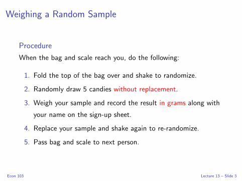
Weighing a Random Sample
Procedure
When the bag and scale reach you, do the following:
1. Fold the top of the bag over and shake to randomize.
2. Randomly draw 5 candies without replacement.
3. Weigh your sample and record the result in grams along with
your name on the sign-up sheet.
4. Replace your sample and shake again to re-randomize.
5. Pass bag and scale to next person.
Econ 103 Lecture 13 – Slide 3

Sampling and Estimation
Questions to Answer
1. How accurately do sample statistics estimate population
parameters?
2. How can we quantify the uncertainty in our estimates?
3. What’s so good about random sampling?
Econ 103 Lecture 13 – Slide 4

Random Sample
In Words
Select sample of n objects from population so that:
1. Each member of the population has the same probability of
being selected
2. The fact that one individual is selected does not affect the
chance that any other individual is selected
3. Each sample of size n is equally likely to be selected
In Math
X1,X2, . . . ,Xn ∼ iid f (x) if continuous
X1,X2, . . . ,Xn ∼ iid p(x) if discrete
Econ 103 Lecture 13 – Slide 5

Random Sample Means Sample With Replacement
I Without replacement ⇒ dependence between samples
I Sample small relative to popn. ⇒ dependence negligible.
I This means our candy experiment (in progress) isn’t bogus.
Econ 103 Lecture 13 – Slide 6

Example: Sampling from Econ 103 Class List
Popn. Mean = 67.5, Popn. Var. = 19.7
Height in Inches
His
togr
am D
ensi
ty
60 65 70 75
0.00
0.02
0.04
0.06
0.08
Use R to illustrate the in an example where we know the
population. Can’t do this in the real applications, but simulate it
on the computer. . .
Econ 103 Lecture 13 – Slide 7

Sampling Distribution of Xn =1n
∑ni=1 Xi
Choose 5 Students from Class List with Replacement
��
���
Sample 1
?
x1
?
Sample 2
?
x2
...
...
@@
@@@R
Sample M
?
xM
Repeat M times → get M different sample means
Sampling Dist: relative frequencies of the xi when M = ∞
Econ 103 Lecture 13 – Slide 8

Height of Econ 103 Students
Popn. Mean = 67.5, Popn. Var. = 19.7
Height in Inches
His
togr
am D
ensi
ty
60 65 70 75
0.00
0.02
0.04
0.06
0.08
Mean = 67.6, Var = 3.6
n = 5
62 64 66 68 70 72 74
050
010
0015
0020
00
Figure: Left: Population, Right: Sampling distribution of X5
Econ 103 Lecture 13 – Slide 9
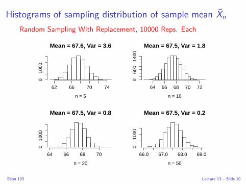
Histograms of sampling distribution of sample mean Xn
Random Sampling With Replacement, 10000 Reps. Each
Mean = 67.6, Var = 3.6
n = 5
62 66 70 74
010
00Mean = 67.5, Var = 1.8
n = 10
64 66 68 70 72
060
014
00
Mean = 67.5, Var = 0.8
n = 20
64 66 68 70
010
00
Mean = 67.5, Var = 0.2
n = 50
66.0 67.0 68.0 69.0
010
00
Econ 103 Lecture 13 – Slide 10

Population Distribution vs. Sampling Distribution of Xn
Popn. Mean = 67.5, Popn. Var. = 19.7
Height in Inches
His
togr
am D
ensi
ty
60 65 70 75
0.00
0.02
0.04
0.06
0.08
Sampling Dist. of Xn
n Mean Variance
5 67.6 3.6
10 67.5 1.8
20 67.5 0.8
50 67.5 0.2
Things to Notice:
1. Sampling dist. “correct on average”
2. Sampling variability decreases with n
3. Sampling dist. bell-shaped even though population isn’t!
Econ 103 Lecture 13 – Slide 11

Step 1: Population as RV rather than List of Objects
Old Way
In the 2016 election, 65,853,625 out of
137,100,229 voters voted for Hillary Clinton
New Way
Bernoulli(p = 0.48) RV
Old Way
List of heights for 97 million US adult males
with mean 69 in and std. dev. 6 in
New Way
N(µ = 69, σ2 = 36) RV
Second example assumes distribution of height is bell-shaped.
Econ 103 Lecture 13 – Slide 12

Step 2: iid RVs Represent Random Sampling from Popn.
Hillary Voters Example
Poll random sample of 1000 people who voted in 2016:
X1, . . . ,X1000 ∼ iid Bernoulli(p = 0.48)
Height Example
Measure the heights of random sample of 50 US males:
Y1, . . . ,Y50 ∼ iid N(µ = 69, σ2 = 36)
Key Question
What do the properties of the population imply about the
properties of the sample?
Econ 103 Lecture 13 – Slide 13

What does the population imply about the sample?
Suppose that exactly half of US voters chose Hillary Clinton in the
2016 election. If you poll a random sample of 4 voters, what is the
probability that exactly half were Hillary supporters?(4
2
)(1/2)2 (1/2)2 = 3/8 = 0.375
Econ 103 Lecture 13 – Slide 14
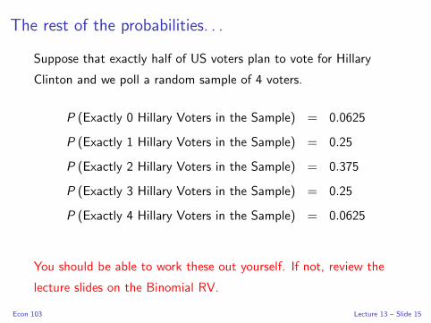
The rest of the probabilities. . .
Suppose that exactly half of US voters plan to vote for Hillary
Clinton and we poll a random sample of 4 voters.
P (Exactly 0 Hillary Voters in the Sample) = 0.0625
P (Exactly 1 Hillary Voters in the Sample) = 0.25
P (Exactly 2 Hillary Voters in the Sample) = 0.375
P (Exactly 3 Hillary Voters in the Sample) = 0.25
P (Exactly 4 Hillary Voters in the Sample) = 0.0625
You should be able to work these out yourself. If not, review the
lecture slides on the Binomial RV.
Econ 103 Lecture 13 – Slide 15

Population Size is Irrelevant Under Random Sampling
Crucial Point
None of the preceding calculations involved the population size: I
didn’t even tell you what it was! We’ll never talk about population
size again in this course.
Why?
Draw with replacement =⇒ only the sample size and the
proportion of Hillary supporters in the population matter.
Econ 103 Lecture 13 – Slide 16

(Sample) Statistic
Any function of the data alone, e.g. sample mean x = 1n
∑ni=1 xi .
Typically used to estimate an unknown population parameter: e.g.
x is an estimate of µ.
Econ 103 Lecture 13 – Slide 17

Step 3: Random Sampling ⇒ Sample Statistics are RVs
This is the crucial point of the course: if we draw a random
sample, the dataset we get is random. Since a statistic is a
function of the data, it is a random variable!
Econ 103 Lecture 13 – Slide 18

A Sample Statistic in the Polling Example
Suppose that exactly half of voters in the population support
Hillary Clinton and we poll a random sample of 4 voters. If we
code Hillary supporters as “1” and everyone else as “0” then what
are the possible values of the sample mean in our dataset?
(a) (0, 1)
(b) {0, 0.25, 0.5, 0.75, 1}
(c) {0, 1, 2, 3, 4}
(d) (−∞,∞)
(e) Not enough information to determine.
Econ 103 Lecture 13 – Slide 19

Sampling Distribution
Under random sampling, a statistic is a RV so it has a PDF if
continuous or PMF if discrete: this is its sampling distribution.
Sampling Dist. of Sample Mean in Polling Example
p(0) = 0.0625
p(0.25) = 0.25
p(0.5) = 0.375
p(0.75) = 0.25
p(1) = 0.0625
Econ 103 Lecture 13 – Slide 20

Contradiction? No, but we need better terminology. . .
I Under random sampling, a statistic is a RV
I Given dataset is fixed so statistic is a constant number
I Distinguish between: Estimator vs. Estimate
Estimator
Description of a general procedure.
Estimate
Particular result obtained from applying the procedure.
Econ 103 Lecture 13 – Slide 21

Xn is an Estimator = Procedure = Random Variable
1. Take a random sample: X1, . . . ,Xn
2. Average what you get: Xn = 1n
∑ni=1 Xi
x is an Estimate = Result of Procedure = Constant
I Result of taking a random sample was the dataset: x1, . . . , xn
I Result of averaging the observed data was x = 1n
∑ni=1 xi
Sampling Distribution of Xn
Thought experiment: suppose I were to repeat the procedure of
taking the mean of a random sample over and over forever. What
relative frequencies would I get for the sample means?
Econ 103 Lecture 13 – Slide 22

Mean of Sampling Distribution of Xn
X1, . . . ,Xn ∼ iid with mean µ
E [Xn] = E
[1
n
n∑i=1
Xi
]=
1
n
n∑i=1
E [Xi ] =1
n
n∑i=1
µ =nµ
n= µ
Hence, sample mean is “correct on average.” The formal term for
this is unbiased.
Econ 103 Lecture 13 – Slide 23
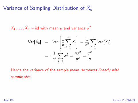
Variance of Sampling Distribution of Xn
X1, . . . ,Xn ∼ iid with mean µ and variance σ2
Var [Xn] = Var
[1
n
n∑i=1
Xi
]=
1
n2
n∑i=1
Var(Xi )
=1
n2
n∑i=1
σ2 =nσ2
n2=
σ2
n
Hence the variance of the sample mean decreases linearly with
sample size.
Econ 103 Lecture 13 – Slide 24

Standard Error
Std. Dev. of estimator’s sampling dist. is called standard error.
Standard Error of the Sample Mean
SE (Xn) =√Var
(Xn
)=√σ2/n = σ/
√n
Econ 103 Lecture 13 – Slide 25

Lecture #14 – Sampling Distributions and Estimation II
Bias of an Estimator
Why divide by n − 1 in sample variance?
Biased Sampling and the Candy-Weighing Experiment
Efficiency: Choosing between Unbiased Estimators
Mean-Squared Error: Choosing Between Biased Estimators
Consistency and the Law of Large Numbers
Econ 103 Lecture 14 – Slide 1
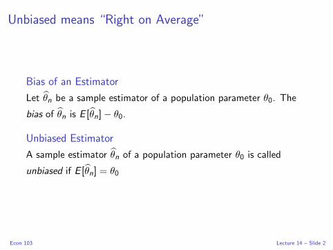
Unbiased means “Right on Average”
Bias of an Estimator
Let θn be a sample estimator of a population parameter θ0. The
bias of θn is E [θn]− θ0.
Unbiased Estimator
A sample estimator θn of a population parameter θ0 is called
unbiased if E [θn] = θ0
Econ 103 Lecture 14 – Slide 2
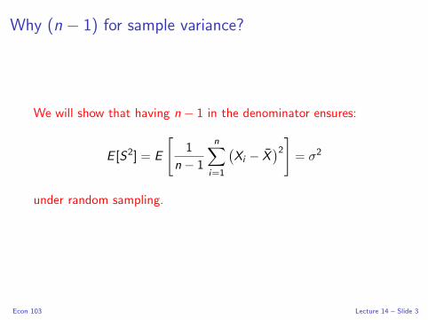
Why (n − 1) for sample variance?
We will show that having n − 1 in the denominator ensures:
E [S2] = E
[1
n − 1
n∑i=1
(Xi − X
)2]= σ2
under random sampling.
Econ 103 Lecture 14 – Slide 3

Why (n − 1) for sample variance?
Step # 1 – Tedious but straightforward algebra gives:
n∑i=1
(Xi − X
)2=
[n∑
i=1
(Xi − µ)2]− n(X − µ)2
You are not responsible for proving Step #1 on an exam.
Econ 103 Lecture 14 – Slide 4

n∑i=1
(Xi − X
)2=
n∑i=1
(Xi − µ+ µ− X
)2=
n∑i=1
[(Xi − µ)− (X − µ)
]2=
n∑i=1
[(Xi − µ)2 − 2(Xi − µ)(X − µ) + (X − µ)2
]=
n∑i=1
(Xi − µ)2 −n∑
i=1
2(Xi − µ)(X − µ) +n∑
i=1
(X − µ)2
=
[n∑
i=1
(Xi − µ)2
]− 2(X − µ)
n∑i=1
(Xi − µ) + n(X − µ)2
=
[n∑
i=1
(Xi − µ)2
]− 2(X − µ)
(n∑
i=1
Xi −n∑
i=1
µ
)+ n(X − µ)2
=
[n∑
i=1
(Xi − µ)2
]− 2(X − µ)(nX − nµ) + n(X − µ)2
=
[n∑
i=1
(Xi − µ)2
]− 2n(X − µ)2 + n(X − µ)2
=
[n∑
i=1
(Xi − µ)2
]− n(X − µ)2
Econ 103 Lecture 14 – Slide 5

Why (n − 1) for sample variance?
Step # 2 – Take Expectations of Step # 1:
E
[n∑
i=1
(Xi − X
)2]= E
[{n∑
i=1
(Xi − µ)2}
− n(X − µ)2
]
= E
[n∑
i=1
(Xi − µ)2]− E
[n(X − µ)2
]=
n∑i=1
E[(Xi − µ)2
]− n E
[(X − µ)2
]Where we have used the linearity of expectation.
Econ 103 Lecture 14 – Slide 6

Why (n − 1) for sample variance?
Step # 3 – Use assumption of random sampling:
X1, . . . ,Xn ∼ iid with mean µ and variance σ2
E
[n∑
i=1
(Xi − X
)2]=
n∑i=1
E[(Xi − µ)2
]− n E
[(X − µ)2
]=
n∑i=1
Var(Xi )− n E[(X − E [X ])2
]=
n∑i=1
Var(Xi )− n Var(X ) = nσ2 − σ2
= (n − 1)σ2
Since we showed earlier today that E [X ] = µ and Var(X ) = σ2/n
under this random sampling assumption.
Econ 103 Lecture 14 – Slide 7

Why (n − 1) for sample variance?
Finally – Divide Step # 3 by (n − 1):
E [S2] = E
[1
n − 1
n∑i=1
(Xi − X
)2]=
(n − 1)σ2
n − 1= σ2
Hence, having (n − 1) in the denominator ensures that the sample
variance is “correct on average,” that is unbiased.
Econ 103 Lecture 14 – Slide 8

A Different Estimator of the Population Variance
σ2 =1
n
n∑i=1
(Xi − X
)2
E [σ2] = E
[1
n
n∑i=1
(Xi − X
)2]=
1
nE
[n∑
i=1
(Xi − X
)2]=
(n − 1)σ2
n
Bias of σ2
E [σ2]− σ2 =(n − 1)σ2
n− σ2 =
(n − 1)σ2
n− nσ2
n= −σ2/n
Econ 103 Lecture 14 – Slide 9

How Large is the Average Family?
How many brothers and sisters are in your family,
including yourself?
Econ 103 Lecture 14 – Slide 10

The average number of children per family was
about 2.0 twenty years ago.
Econ 103 Lecture 14 – Slide 11
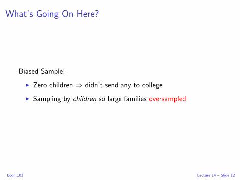
What’s Going On Here?
Biased Sample!
I Zero children ⇒ didn’t send any to college
I Sampling by children so large families oversampled
Econ 103 Lecture 14 – Slide 12
Candy Weighing: 49 Estimates, Each With n = 5
θ = 20× (X1 + . . .+ X5)
Summary of Sampling Dist.
Overestimates 45
Exactly Correct 0
Underestimates 4
E [θ] 1164 grams
SD(θ) 189 grams
Actual Mass: θ0 =932 grams
Histogram
Est. Weight of All Candies (grams)
Fre
quen
cy800 1000 1400
05
1015
Econ 103 Lecture 14 – Slide 13

What was in the bag?
100 Candies Total:
I 20 Fun Size Snickers Bars (large)
I 30 Reese’s Miniatures (medium)
I 50 Tootsie Roll “Midgees” (small)
So What Happened?
Not a random sample! The Snickers bars were oversampled.
Could we have avoided this? How?
Econ 103 Lecture 14 – Slide 14

Let X1,X2, . . .Xn ∼ iid mean µ, variance σ2 and define
Xn = 1n
∑ni=1 Xi . True or False:
Xn is an unbiased estimator of µ
(a) True
(b) False
TRUE!
Econ 103 Lecture 14 – Slide 15

Let X1,X2, . . .Xn ∼ iid mean µ, variance σ2. True or False:
X1 is an unbiased estimator of µ
(a) True
(b) False
TRUE!
Econ 103 Lecture 14 – Slide 16

How to choose between two unbiased estimators?
Suppose X1,X2, . . .Xn ∼ iid with mean µ and variance σ2
E [Xn] = E
[1
n
n∑i=1
Xi
]=
1
n
n∑i=1
E [Xi ] = µ
E [X1] = µ
Var(Xn) = Var
(1
n
n∑i=1
Xi
)=
1
n2
n∑i=1
Var(Xi ) = σ2/n
Var(X1) = σ2
Econ 103 Lecture 14 – Slide 17

Efficiency - Compare Unbiased Estimators by Variance
Let θ1 and θ2 be unbiased estimators of θ0. We say that θ1 is more
efficient than θ2 if Var(θ1) < Var(θ2).
Econ 103 Lecture 14 – Slide 18

Mean-Squared Error
Except in very simple situations, unbiased estimators are hard to
come by. In fact, in many interesting applications there is a
tradeoff between bias and variance:
I Low bias estimators often have a high variance
I Low variance estimators often have high bias
Mean-Squared Error (MSE): Squared Bias plus Variance
MSE (θ) = Bias(θ)2 + Var(θ)
Root Mean-Squared Error (RMSE):√MSE
Econ 103 Lecture 14 – Slide 19
Calculate MSE for Candy Experiment
Histogram
Est. Weight of All Candies (grams)
Fre
quen
cy
800 1000 1200 1400 1600
05
1015
E [θ] 1164 grams
θ0 932 grams
SD(θ) 189 grams
Bias = 1164 grams− 932 grams
= 232 grams
MSE = Bias2 + Variance
= (2322 + 1892) grams2
= 8.9545× 10⁴ grams2
RMSE =√MSE = 299 grams
Econ 103 Lecture 14 – Slide 20

Finite Sample versus Asymptotic Properties of Estimators
Finite Sample Properties
For fixed sample size n what are the properties of the sampling
distribution of θn? (E.g. bias and variance.)
Asymptotic Properties
What happens to the sampling distribution of θn as the sample size
n gets larger and larger? (That is, n → ∞).
Econ 103 Lecture 14 – Slide 21

Why Asymptotics?
Law of Large Numbers
Make precise what we mean by “bigger samples are better.”
Central Limit Theorem
As n → ∞ pretty much any sampling distribution is
well-approximated by a normal random variable!
Econ 103 Lecture 14 – Slide 22

Consistency
Consistency
If an estimator θn (which is a RV) converges to θ0 (a constant) as
n → ∞, we say that θn is consistent for θ0.
What does it mean for a RV to converge to a constant?
For this course we’ll use MSE Consistency:
limn→∞
MSE(θn) = 0
This makes sense since MSE(θn) is a constant, so this is just an
ordinary limit from calculus.
Econ 103 Lecture 14 – Slide 23
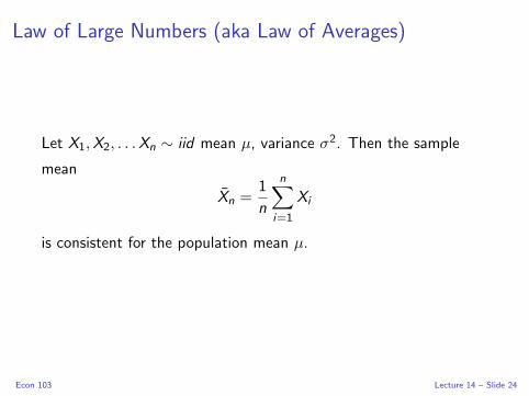
Law of Large Numbers (aka Law of Averages)
Let X1,X2, . . .Xn ∼ iid mean µ, variance σ2. Then the sample
mean
Xn =1
n
n∑i=1
Xi
is consistent for the population mean µ.
Econ 103 Lecture 14 – Slide 24

Law of Large Numbers (aka Law of Averages)
Let X1,X2, . . .Xn ∼ iid mean µ, variance σ2.
E [Xn] = E
[1
n
n∑i=1
Xi
]= µ
Var(Xn) = Var
(1
n
n∑i=1
Xi
)= σ2/n
MSE(Xn) = Bias(Xn)2 + Var(Xn)
=(E [Xn]− µ
)2+ Var(Xn)
= 0 + σ2/n
→ 0
Hence Xn is consistent for µEcon 103 Lecture 14 – Slide 25

Important!
An estimator can be biased but still consistent, as long as the bias
disappears as n → ∞
σ2 =1
n
n∑i=1
(Xi − X
)2
Bias of σ2
E [σ2]− σ2 =(n − 1)σ2
n− σ2 = − σ2/n → 0
Econ 103 Lecture 14 – Slide 26

Suppose X1,X2, . . . ,Xn ∼ iid N(µ, σ2). What is the sampling
distribution of Xn?
(a) N(0, 1)
(b) N(µ, σ2/n)
(c) N(µ, σ2)
(d) N(µ/n, σ2/n)
(e) N(nµ, nσ2)
Econ 103 Lecture 14 – Slide 27

But still, how can something random
converge to something constant?
Econ 103 Lecture 14 – Slide 28
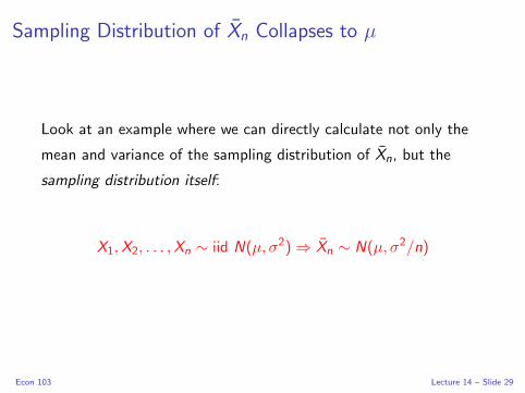
Sampling Distribution of Xn Collapses to µ
Look at an example where we can directly calculate not only the
mean and variance of the sampling distribution of Xn, but the
sampling distribution itself:
X1,X2, . . . ,Xn ∼ iid N(µ, σ2) ⇒ Xn ∼ N(µ, σ2/n)
Econ 103 Lecture 14 – Slide 29

Sampling Distribution of Xn Collapses to µ
X1,X2, . . . ,Xn ∼ iid N(µ, σ2 ⇒ Xn ∼ N(µ, σ2/n).
−4 −2 0 2 4
01
23
4
n = 1
−4 −2 0 2 4
01
23
4
n = 10
−4 −2 0 2 4
01
23
4
n = 50
−4 −2 0 2 4
01
23
4
n = 100
Figure: Sampling Distributions for Xn where Xi ∼ iid N(0, 1)Econ 103 Lecture 14 – Slide 30
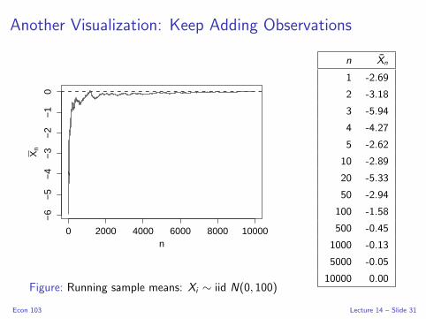
Another Visualization: Keep Adding Observations
0 2000 4000 6000 8000 10000
−6
−5
−4
−3
−2
−1
0
n
Xn
Figure: Running sample means: Xi ∼ iid N(0, 100)
n Xn
1 -2.69
2 -3.18
3 -5.94
4 -4.27
5 -2.62
10 -2.89
20 -5.33
50 -2.94
100 -1.58
500 -0.45
1000 -0.13
5000 -0.05
10000 0.00
Econ 103 Lecture 14 – Slide 31

Lecture #15 – Confidence Intervals I
Confidence Interval for Mean of Normal Population (σ2 Known)
Interpreting a Confidence Interval
Margin of Error and Width
Econ 103 Lecture 15 – Slide 1

Today – Simplest Example of a Confidence Interval
I Suppose the population is N(µ, σ2)
I We know σ2 but not µ
I Draw random sample X1,X2, . . . ,Xn ∼ iid N(µ, σ2)
I Observe value of sample mean xn (e.g. 69 inches)
I What is a plausible range for µ?
I How confident are we? Can we make this precise?
Next time we’ll look at more realistic and interesting examples. . .
Econ 103 Lecture 15 – Slide 2

Suppose X1,X2, . . . ,Xn ∼ iid N(µ, σ2). What is the sampling
distribution of√n(Xn − µ)/σ?
(a) N(µ, σ2)
(b) N(0, 1)
(c) N(0, σ)
(d) N(µ, 1)
(e) Not enough information to determine.
Econ 103 Lecture 15 – Slide 3
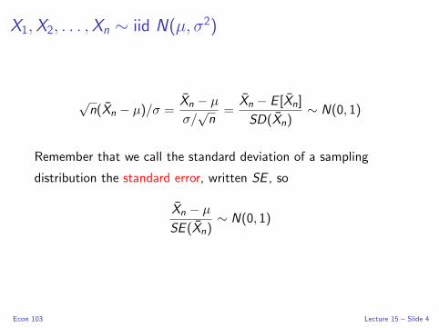
X1,X2, . . . ,Xn ∼ iid N(µ, σ2)
√n(Xn − µ)/σ =
Xn − µ
σ/√n
=Xn − E [Xn]
SD(Xn)∼ N(0, 1)
Remember that we call the standard deviation of a sampling
distribution the standard error, written SE , so
Xn − µ
SE (Xn)∼ N(0, 1)
Econ 103 Lecture 15 – Slide 4

What happens if I rearrange?
P
(−2 ≤ Xn − µ
SE (Xn)≤ 2
)= 0.95
P(−2 · SE ≤ Xn − µ ≤ 2 · SE
)= 0.95
P(−2 · SE − Xn ≤ −µ ≤ 2 · SE − Xn
)= 0.95
P(Xn − 2 · SE ≤ µ ≤ Xn + 2 · SE
)= 0.95
Econ 103 Lecture 15 – Slide 5

Confidence Intervals
Confidence Interval (CI)
Range (A,B) constructed from the sample data with specified
probability of containing a population parameter:
P(A ≤ θ0 ≤ B) = 1− α
Confidence Level
The specified probability, typically denoted 1− α, is called the
confidence level. For example, if α = 0.05 then the confidence
level is 0.95 or 95%.
Econ 103 Lecture 15 – Slide 6

Confidence Interval for Mean of Normal PopulationPopulation Variance Known
The interval Xn ± 2σ/√n has approximately 95% probability of
containing the population mean µ, provided that:
X1,X2, . . . ,Xn ∼ iid N(µ, σ2)
But how are we supposed to interpret this?
Econ 103 Lecture 15 – Slide 7

Confidence Interval is a Random Variable!
1. X1, . . . ,Xn are RVs ⇒ Xn is a RV (repeated sampling)
2. µ, σ and n are constants
3. Confidence Interval Xn ± 2σ/√n is also a RV!
Econ 103 Lecture 15 – Slide 8

Meaning of Confidence Interval
Formal Meaning
If we sampled many times we’d get many different sample means,
each leading to a different confidence interval. Approximately 95%
of these intervals will contain µ.
Rough Intuition
What values of µ are consistent with the data?
Econ 103 Lecture 15 – Slide 9

CI for Population Mean: Repeated Sampling
X1,X2, . . . ,Xn ∼ iid N(µ, σ2)
��
���
Sample 1
?
x1
?
x1 ± 2σ/√n
?
Sample 2
?
x2
?
x2 ± 2σ/√n
...
...
@@
@@@R
Sample M
?
xM
?
xM ± 2σ/√n
Repeat M times → get M different intervals
Large M ⇒ Approx. 95% of these Intervals Contain µ
Econ 103 Lecture 15 – Slide 10

Simulation Example: X1, . . . ,X5 ∼ iid N(0, 1), M = 20
●
●
●
●
●
●
●
●
●
●
●
●
●
●
●
●
●
●
●
●
−1.0 −0.5 0.0 0.5 1.0 1.5 2.0
Xn
Figure: Twenty confidence intervals of the form Xn ± 2σ/√n where
n = 5, σ2 = 1 and the true population mean is 0.Econ 103 Lecture 15 – Slide 11

Meaning of Confidence Interval for θ0
P(A ≤ θ0 ≤ B) = 1− α
Each time we sample we’ll get a different confidence interval,
corresponding to different realizations of the random variables A
and B. If we sample many times, approximately 100× (1− α)% of
these intervals will contain the population parameter θ0.
Econ 103 Lecture 15 – Slide 12

Confidence Intervals: Some Terminology
Margin of Error
When a CI takes the form θ ±ME , ME is the Margin of Error.
Lower and Upper Confidence Limits
The lower endpoint of a CI is the lower confidence limit (LCL),
while the upper endpoint is the upper confidence limit (UCL).
Width of a Confidence Interval
The distance |UCL− LCL| is called the width of a CI. This means
exactly what it says.
Econ 103 Lecture 15 – Slide 13

What is the Margin of Error
In the preceding example of a 95% confidence interval for the
mean of a normal population when the population variance is
known, which of these is the margin of error?
(a) σ/√n
(b) Xn
(c) σ
(d) 2σ/√n
(e) 1/√n
2σ/√n, since the CI is Xn ± 2σ/
√n
Econ 103 Lecture 15 – Slide 14

What is the Width?
In the preceding example of a 95% confidence interval for the
mean of a normal population when the population variance is
known, which of these is the width of the interval?
(a) σ/√n
(b) 2σ/√n
(c) 3σ/√n
(d) 4σ/√n
(e) 5σ/√n
4σ/√n, since the CI is Xn ± 2σ/
√n
Econ 103 Lecture 15 – Slide 15

Example: Calculate the Margin of Error
X1, . . . ,X100 ∼ iid N(µ, 1) but we don’t know µ.
Want to create a 95% confidence interval for µ.
What is the margin of error?
The confidence interval is Xn ± 2σ/√n so
ME = 2σ/√n = 2 · 1/
√100 = 2/10 = 0.2
Econ 103 Lecture 15 – Slide 16

Example: Calculate the Lower Confidence Limit
X1, . . . ,X100 ∼ N(µ, 1) but we don’t know µ.
Want to create a 95% confidence interval for µ.
We found that ME = 0.2. The sample mean x = 4.9. What is the
lower confidence limit?
LCL = x −ME = 4.9− 0.2 = 4.7
Econ 103 Lecture 15 – Slide 17

Example: Similarly for the Upper Confidence Limit. . .
X1, . . . ,X100 ∼ N(µ, 1) but we don’t know µ.
Want to create a 95% confidence interval for µ.
We found that ME = 0.2. The sample mean x = 4.9. What is the
upper confidence limit?
UCL = x +ME = 4.9 + 0.2 = 5.1
Econ 103 Lecture 15 – Slide 18
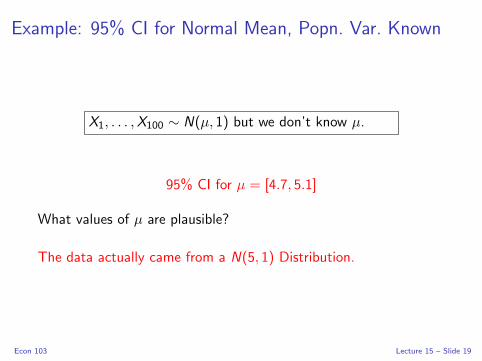
Example: 95% CI for Normal Mean, Popn. Var. Known
X1, . . . ,X100 ∼ N(µ, 1) but we don’t know µ.
95% CI for µ = [4.7, 5.1]
What values of µ are plausible?
The data actually came from a N(5, 1) Distribution.
Econ 103 Lecture 15 – Slide 19
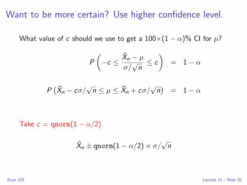
Want to be more certain? Use higher confidence level.
What value of c should we use to get a 100×(1− α)% CI for µ?
P
(−c ≤ Xn − µ
σ/√n
≤ c
)= 1− α
P(Xn − cσ/
√n ≤ µ ≤ Xn + cσ/
√n)
= 1− α
Take c = qnorm(1− α/2)
Xn ± qnorm(1− α/2)× σ/√n
Econ 103 Lecture 15 – Slide 20

−4 −2 0 2 4
0.0
0.1
0.2
0.3
0.4
x
f(x)
Econ 103 Lecture 15 – Slide 21
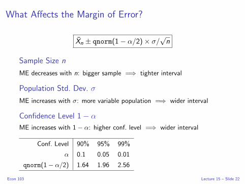
What Affects the Margin of Error?
Xn ± qnorm(1− α/2)× σ/√n
Sample Size n
ME decreases with n: bigger sample =⇒ tighter interval
Population Std. Dev. σ
ME increases with σ: more variable population =⇒ wider interval
Confidence Level 1− α
ME increases with 1− α: higher conf. level =⇒ wider interval
Conf. Level 90% 95% 99%
α 0.1 0.05 0.01
qnorm(1− α/2) 1.64 1.96 2.56
Econ 103 Lecture 15 – Slide 22

Lecture #16 – Confidence Intervals II
Comparing intervals with different confidence levels
What if the population is normal but σ is unknown?
What if the population isn’t normal? – The Central Limit Theorem
CI for a Proportion Using the Central Limit Theorem
Econ 103 Lecture 16 – Slide 1

Xn − 3SE Xn + 3SE
99.7%
Xn − 2SE Xn + 2SE
95%
Xn − SE Xn + SE
68%
Xn
Figure: Each CI gives a range of “plausible” values for the population mean µ,centered at the sample mean Xn. Values near the middle are “more plausible”in the sense that a small reduction in confidence level gives a much shorterinterval centered in the same place. This is because the sample mean isunlikely to take on values far from the population mean in repeated sampling.
Econ 103 Lecture 16 – Slide 2

Assume that: X1, . . . ,Xn ∼ iid N(µ, σ2)
σ Known
P
[−qnorm(1− α/2) ≤ Xn − µ
σ/√n
≤ qnorm(1− α/2)
]= 1− α
=⇒ Confidence Interval: Xn ± qnorm(1− α/2)× σ/√n
σ Unknown
Idea: estimate σ with S . Unfortunately:
Xn − µ
S/√n
IS NOT A NORMAL RV!
Econ 103 Lecture 16 – Slide 3
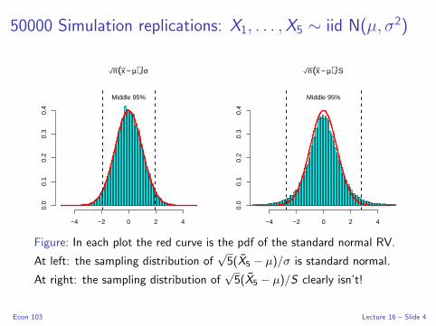
50000 Simulation replications: X1, . . . ,X5 ∼ iid N(µ, σ2)
−4 −2 0 2 4
0.0
0.1
0.2
0.3
0.4
n(x − µ) σ
Middle 95%
−4 −2 0 2 4
0.0
0.1
0.2
0.3
0.4
n(x − µ) S
Middle 95%
Figure: In each plot the red curve is the pdf of the standard normal RV.
At left: the sampling distribution of√5(X5 − µ)/σ is standard normal.
At right: the sampling distribution of√5(X5 − µ)/S clearly isn’t!
Econ 103 Lecture 16 – Slide 4

Student-t Random Variable
If X1, . . . ,Xn ∼ iid N(µ, σ2), then
Xn − µ
S/√n
∼ t(n − 1)
I Parameter: ν = n − 1 “degrees of freedom”
I Support = (−∞,∞)
I Symmetric around zero, but mean and variance may not exist!
I Degrees of freedom ν control “thickness of tails”
I As ν → ∞, t → Standard Normal.
Econ 103 Lecture 16 – Slide 5

Student-t PDFs
−4 −2 0 2 4
0.0
0.1
0.2
0.3
0.4
x
f(x)
ν = ∞ν = 3ν = 1
Econ 103 Lecture 16 – Slide 6

Who was “Student?”“Guinnessometrics: The Economic Foundation of Student’s t”
“Student” is the pseudonym used in 19 of 21
published articles by William Sealy Gosset, who
was a chemist, brewer, inventor, and self-trained
statistician, agronomer, and designer of
experiments ... [Gosset] worked his entire adult
life ... as an experimental brewer for one
employer: Arthur Guinness, Son & Company,
Ltd., Dublin, St. Jamess Gate. Gosset was a
master brewer and rose in fact to the top of the
top of the brewing industry: Head Brewer of
Guinness.
Econ 103 Lecture 16 – Slide 7

CI for Mean of Normal Distribution, Popn. Var. Unknown
Same argument as we used when the variance was known, except
with t(n − 1) rather than standard normal distribution:
P
(−c ≤ Xn − µ
S/√n
≤ c
)= 1− α
P
(Xn − c
S√n≤ µ ≤ Xn + c
S√n
)= 1− α
c = qt(1− α/2, df = n − 1)
Xn ± qt(1− α/2, df = n − 1)S√n
Econ 103 Lecture 16 – Slide 8

Comparison of CIs for Mean of Normal Distribution100× (1− α)% Confidence Level
X1, . . . ,Xn ∼ iid N(µ, σ2)
Known Population Std. Dev. (σ)
Xn ± qnorm(1− α/2)σ√n
Unknown Population Std. Dev. (σ)
Xn ± qt(1− α/2, df = n − 1)S√n
Econ 103 Lecture 16 – Slide 9

Comparison of Normal and t CIs
Table: Values of qt(1− α/2, df = n − 1) for various choices of n and α.
n 1 5 10 30 100 ∞α = 0.10 6.31 2.02 1.81 1.70 1.66 1.64
α = 0.05 12.71 2.57 2.23 2.04 1.98 1.96
α = 0.01 63.66 4.03 3.17 2.75 2.63 2.58
As n → ∞, t(n − 1) → N(0, 1)
In a sense, using the t-distribution involves making a “small-sample
correction.” In other words, it is only when n is fairly small that
this makes a practical difference for our confidence intervals.
Econ 103 Lecture 16 – Slide 10

Am I Taller Than The Average American Male?
Source: Centers for Disease Control (pg. 16)
Sample Mean 69 inches
Sample Std. Dev. 6 inches
Sample Size 5647
My Height 73 inches
SE(Xn) = s/√n
= 6/√5647
≈ 0.08
Assuming the population is normal,
Xn ± qt(1− α/2, df = n − 1) SE (Xn)
What is the approximate value of
qt(1-0.05/2, df = 5646)?
For large n, t(n − 1) ≈ N(0, 1), so the
answer is approximately 2
What is the ME for the 95% CI?
ME ≈ 0.16 =⇒ 69± 0.16
Econ 103 Lecture 16 – Slide 11

The Central Limit Theorem
Suppose that X1, . . . ,Xn are a random sample from a some
population that is not necessarily normal and has an unknown
mean µ. Then, provided that n is sufficiently large,
Xn − µ
S/√n
≈ N(0, 1)
We will use this fact to create approximate CIs for population
mean even if we know nothing about the population.
Econ 103 Lecture 16 – Slide 12

Example: Uniform(0,1) Population, n = 20
0.0 0.2 0.4 0.6 0.8 1.0
0.0
0.5
1.0
1.5
Uniform Population
x
f(x)
Sample Mean − Uniform Pop (n = 20)
0.3 0.4 0.5 0.6 0.7 0.80
500
1500
2500
Econ 103 Lecture 16 – Slide 13

Example: χ2(5) Population, n = 20
0 5 10 15 20 25
0.00
0.05
0.10
0.15
Chi−squared(5) Population
x
f(x)
Sample Mean − Chisq(5) Pop (n=20)
2 3 4 5 6 7 80
500
1500
2500
Econ 103 Lecture 16 – Slide 14
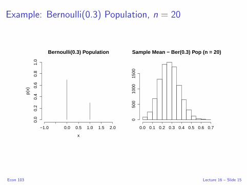
Example: Bernoulli(0.3) Population, n = 20
−1.0 0.0 0.5 1.0 1.5 2.0
0.0
0.2
0.4
0.6
0.8
1.0
Bernoulli(0.3) Population
x
p(x)
Sample Mean − Ber(0.3) Pop (n = 20)
0.0 0.1 0.2 0.3 0.4 0.5 0.6 0.70
500
1000
1500
Econ 103 Lecture 16 – Slide 15

Are US Voters Really That Ignorant?Pew: “What Voters Know About Campaign 2012”
The Data
Of 771 registered voters polled, only 39% correctly identified John
Roberts as the current chief justice of the US Supreme Court.
Research Question
Is the majority of voters unaware that John Roberts is the current
chief justice, or is this just sampling variation?
Assume Random Sampling...
Econ 103 Lecture 16 – Slide 16

Confidence Interval for a Proportion
What is the appropriate probability model for the sample?
X1, . . . ,Xn ∼ iid Bernoulli(p), 1 = Know Roberts is Chief Justice
What is the parameter of interest?
p = Proportion of voters in the population who know Roberts is
Chief Justice.
What is our estimator?
Sample Proportion: p = (∑n
i=1 Xi )/n
Econ 103 Lecture 16 – Slide 17

Sample Proportion is the Sample Mean!
X1, . . . ,Xn ∼ iid Bernoulli(p)
p =1
n
n∑i=1
Xi = Xn
E [p] = E
(1
n
n∑i=1
Xi
)=
1
n
n∑i=1
E [Xi ] =np
n= p
Var(p) = Var
(1
n
n∑i=1
Xi
)=
1
n2
n∑i=1
Var(Xi ) =np(1− p)
n2=
p(1− p)
n
SE (p) =√Var(p) =
√p(1− p)
n
SE (p) =
√p(1− p)
nEcon 103 Lecture 16 – Slide 18

Central Limit Theorem Applied to Sample Proportion
Central Limit Theorem: Intuition
Sample means are approximately normally distributed provided the
sample size is large even if the population is non-normal.
CLT For Sample Mean
Xn − µ
S/√n
≈ N(0, 1)
CLT for Sample Proportion
p − p√p(1−p)
n
≈ N(0, 1)
In this example, the population is Bernoulli(p) rather than normal.
The sample mean is p and the population mean is p.
Econ 103 Lecture 16 – Slide 19

Approximate 95% CI for Population Proportion
p − p√p(1−p)
n
≈ N(0, 1)
P
−2 ≤ p − p√p(1−p)
n
≤ 2
≈ 0.95
P
(p − 2
√p(1− p)
n≤ p ≤ p + 2
√p(1− p)
n
)≈ 0.95
Econ 103 Lecture 16 – Slide 20

100× (1− α) CI for Population Proportion (p)
X1, . . . ,Xn ∼ iid Bernoulli(p)
p ± qnorm(1− α/2)
√p(1− p)
n
Approximation based on the CLT. Works well provided n is large
and p isn’t too close to zero or one.
Econ 103 Lecture 16 – Slide 21

Example: Bernoulli(0.9) Population, n = 20
−1.0 0.0 0.5 1.0 1.5 2.0
0.0
0.2
0.4
0.6
0.8
1.0
Bernoulli(0.9) Population
x
p(x)
Sample Mean − Ber(0.9) Pop (n = 20)
0.6 0.7 0.8 0.9 1.00
500
1500
2500
Econ 103 Lecture 16 – Slide 22
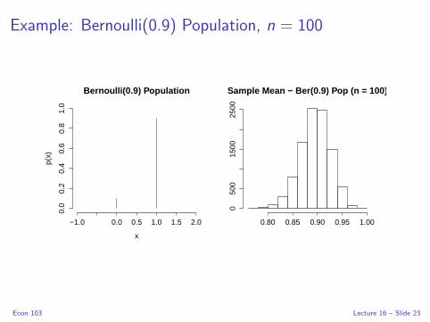
Example: Bernoulli(0.9) Population, n = 100
−1.0 0.0 0.5 1.0 1.5 2.0
0.0
0.2
0.4
0.6
0.8
1.0
Bernoulli(0.9) Population
x
p(x)
Sample Mean − Ber(0.9) Pop (n = 100)
0.80 0.85 0.90 0.95 1.000
500
1500
2500
Econ 103 Lecture 16 – Slide 23

Approximate 95% CI for Population Proportion
39% of 771 Voters Polled Correctly Identified Chief Justice Roberts
SE (p) =
√p(1− p)
n=
√(0.39)(0.61)
771≈ 0.018
What is the ME for an approximate 95% confidence interval?
ME ≈ 2× SE (Xn) ≈ 0.04
What can we conclude?
Approximate 95% CI: (0.35, 0.43)
Econ 103 Lecture 16 – Slide 24

Lecture #17 – Confidence Intervals III
Sampling Dist. of (X − Y ) – Normal Populations, Variances Known
CI for Difference of Population Means Using CLT
CI for Difference of Population Proportions Using CLT
Matched Pairs versus Independent Samples
Econ 103 Lecture 17 – Slide 1

Sampling Dist. of (Xn − Ym) – Normal Popns. Vars. Known
Suppose X1, . . . ,Xn ∼ iid N(µx , σ2x) indep. of Y1, . . . ,Ym ∼ iid N(µy , σ
2y )
SE (Xn − Ym) =
√σ2x
n+
σ2y
m(Xn − Ym
)− (µx − µy )
SE (Xn − Ym)∼ N(0, 1)
You should be able to prove this using what we’ve learned about RVs.
Econ 103 Lecture 17 – Slide 2

CI for (µX − µY ) – Indep. Normal Popns. σ2X , σ
2Y Known
(Xn − Ym)± qnorm(1− α/2) SE (Xn − Ym)
SE (Xn − Ym) =
√σ2x
n+
σ2y
m
Econ 103 Lecture 17 – Slide 3

CI for Difference of Population Means Using CLT
Setup: Independent Random Samples
X1, . . . ,Xn ∼ iid with unknown mean µX & unknown variance σ2X
Y1, . . . ,Ym ∼ iid with unknown mean µY & unknown variance σ2Y
where each sample is independent of the other
We Do Not Assume the Populations are Normal!
Econ 103 Lecture 17 – Slide 4

Difference of Sample Means Xn − Ym and the CLT
What We Have
Approx. sampling dist. for individual sample means from CLT:
Xn ≈ N(µX , S
2X/n
), Ym ≈ N
(µY , S
2Y /m
)What We Want
Sampling Distribution of the difference Xn − Ym
Use Independence of the Two Samples
Xn − Ym ≈ N
(µX − µY ,
S2X
n+
S2Y
m
)
Econ 103 Lecture 17 – Slide 5
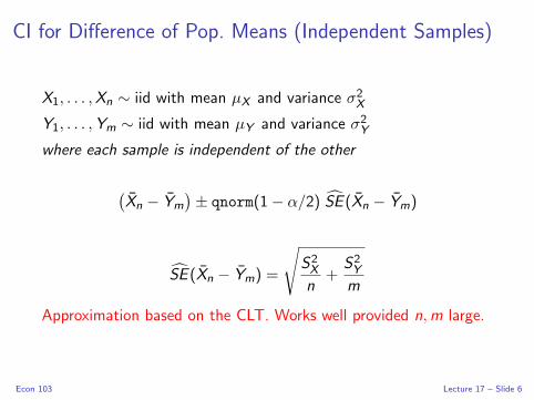
CI for Difference of Pop. Means (Independent Samples)
X1, . . . ,Xn ∼ iid with mean µX and variance σ2X
Y1, . . . ,Ym ∼ iid with mean µY and variance σ2Y
where each sample is independent of the other
(Xn − Ym
)± qnorm(1− α/2) SE (Xn − Ym)
SE (Xn − Ym) =
√S2X
n+
S2Y
m
Approximation based on the CLT. Works well provided n,m large.
Econ 103 Lecture 17 – Slide 6

The Anchoring Experiment
At the beginning of the semester you were each shown a “random
number.” In fact the numbers weren’t random: there was a “Hi”
group that was shown 65 and a “Lo” group that was shown 10.
You were randomly assigned to one of these two groups and shown
your “random” number. You were then asked what proportion of
UN member states are located in Africa.
Econ 103 Lecture 17 – Slide 7

Past Semester’s Anchoring Experiment
10 65
010
2030
4050
60
Anchoring Experiment
Ans
wer
“Lo” Group – Shown 10
mLo = 43
yLo = 17.1
s2Lo = 86
“Hi” Group – Shown 65
nHi = 46
xHi = 30.7
s2Hi = 253
Econ 103 Lecture 17 – Slide 8

ME for approx. 95% for Difference of Means
“Lo” Group
yLo = 17.1
mLo = 43
s2Lo = 86
SE (yLo)2 =
s2LomLo
= 2
“Hi” Group
xHi = 30.7
nHi = 46
s2Hi = 253
SE (xHi )2 =
s2HinHi
= 5.5
XHi − YLo = 30.7− 17.1 = 13.6
SE (XHi − YLo) =
√SE (XHi )2 + SE (YLo)2 =
√7.5 ≈ 2.7 ⇒ ME ≈ 5.4
Approximate 95% CI (8.2, 19) What can we conclude?
Econ 103 Lecture 17 – Slide 9

Confidence Interval for a Difference of Proportions via CLT
What is the appropriate probability model for the sample?
X1, . . . ,Xn ∼ iid Bernoulli(p) independently of
Y1, . . . ,Ym ∼ iid Bernoulli(q)
What is the parameter of interest?
The difference of population proportions p − q
What is our estimator?
The difference of sample proportions: p − q where:
p =1
n
n∑i=1
Xi q =1
m
m∑i=1
Yi
Econ 103 Lecture 17 – Slide 10
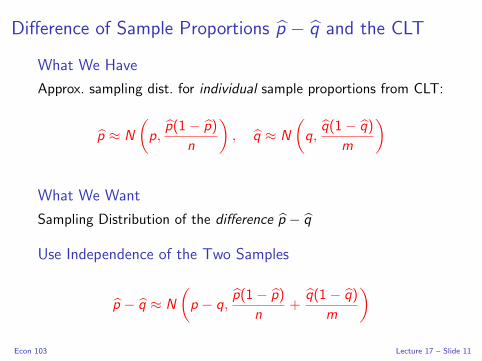
Difference of Sample Proportions p − q and the CLT
What We Have
Approx. sampling dist. for individual sample proportions from CLT:
p ≈ N
(p,
p(1− p)
n
), q ≈ N
(q,
q(1− q)
m
)
What We Want
Sampling Distribution of the difference p − q
Use Independence of the Two Samples
p − q ≈ N
(p − q,
p(1− p)
n+
q(1− q)
m
)Econ 103 Lecture 17 – Slide 11

Approximate CI for Difference of Popn. Proportions (p− q)
X1, . . . ,Xn ∼ iid Bernoulli(p)
Y1, . . . ,Ym ∼ iid Bernoulli(q)
where each sample is independent of the other
(p − q)± qnorm(1− α/2) SE (p − q)
SE (p − q) =
√p(1− p)
n+
q(1− q)
m
Approximation based on the CLT. Works well provided n,m large
and p, q aren’t too close to zero or one.
Econ 103 Lecture 17 – Slide 12
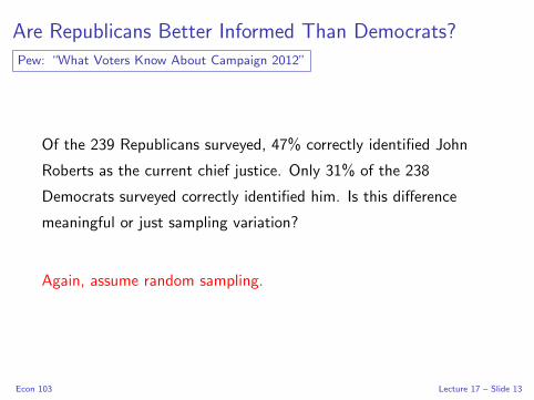
Are Republicans Better Informed Than Democrats?Pew: “What Voters Know About Campaign 2012”
Of the 239 Republicans surveyed, 47% correctly identified John
Roberts as the current chief justice. Only 31% of the 238
Democrats surveyed correctly identified him. Is this difference
meaningful or just sampling variation?
Again, assume random sampling.
Econ 103 Lecture 17 – Slide 13

ME for approx. 95% for Difference of Proportions
47% of 239 Republicans vs. 31% of 238 Democrats identified Roberts
Republicans
p = 0.47
n = 239
SE(p) =
√p(1− p)
n≈ 0.032
Democrats
q = 0.31
m = 238
SE(q) =
√q(1− q)
m≈ 0.030
Difference: (Republicans - Democrats)
p − q = 0.47− 0.31 = 0.16
SE(p − q) =
√SE(p)2 + SE(q)2 ≈ 0.044 =⇒ ME ≈ 0.09
Approximate 95% CI (0.07, 0.25) What can we conclude?
Econ 103 Lecture 17 – Slide 14

Which is the Harder Exam?
Here are the scores from two midterms:
Student Exam 1 Exam 2 Difference
1 57.1 60.7 3.6
2 77.1 77.9 0.7
3 83.6 93.6 10.0...
......
...
69 75.0 74.3 −0.7
70 96.4 86.4 −10.0
71 78.6 82.9 4.3
Sample Mean: 79.6 81.4 1.8
Is it true that students score, on average, better on Exam 2 or is
this just sampling variation?
Econ 103 Lecture 17 – Slide 15

Are the two samples independent?
Suppose we treat the scores on the first midterm as one sample
and the scores on the second as another. Are these samples
independent?
(a) Yes
(b) No
(c) Not Sure
Econ 103 Lecture 17 – Slide 16

Matched Pairs Data – Dependent Samples
The samples are dependent: each includes the same students:
Student Exam 1 Exam 2 Difference
1 57.1 60.7 3.6...
......
...
71 78.6 82.9 4.3
Sample Mean: 79.6 81.4 1.8
Sample Corr. 0.54
This is really a one-sample problem if we consider the difference
between each student’s score on Exam 2 and Exam 1. This setup
is referred to as matched pairs data.
Econ 103 Lecture 17 – Slide 17

Solving this as a One-Sample Problem
Let Di = Xi − Yi be the difference of student i ’s exam scores.
I calculated the following in R:
Dn =1
n
n∑i=1
Di ≈ 1.8
S2D =
1
n − 1
n∑i=1
(Di − D)2 ≈ 124
SE (Dn) = (SD/√n) ≈
√124/71 ≈ 1.3
Approximate 95% CI Based on the CLT:
1.8± 2.6 = (−0.8, 4.4) What is our conclusion?
Econ 103 Lecture 17 – Slide 18

How are the Independent
Samples and Matched Pairs
Problems Related?
Econ 103 Lecture 17 – Slide 19

Difference of Means = Mean of Differences?
Let Di = Xi − Yi be the difference of student i ’s exam scores.
True or False:
Dn = Xn − Yn
(a) True
(b) False
(c) Not Sure
Econ 103 Lecture 17 – Slide 20

Difference of Means Equals Mean of Differences
Dn =1
n
n∑i=1
Di =1
n
n∑i=1
(Xi − Yi ) = Xn − Yn
Student Exam 1 Exam 2 Difference
1 57.1 60.7 3.6...
......
...
71 78.6 82.9 4.3
Sample Mean: 79.6 81.4 1.8
Dn = 1.8
Xn − Yn = 81.4− 79.6 = 1.8 X
Econ 103 Lecture 17 – Slide 21

...But Correlation Affects the Variance
S2D =
1
n − 1
n∑i=1
(Di − Dn
)2=
1
n − 1
n∑i=1
[(Xi − Yi )−
(Xn − Yn
)]2=
1
n − 1
n∑i=1
[(Xi − Xn
)−
(Yi − Yn
)]2=
1
n − 1
n∑i=1
[(Xi − Xn
)2+
(Yi − Yn
)2 − 2(Xi − Xn
) (Yi − Yn
)]= S2
X + S2Y − 2SXY
= S2X + S2
Y − 2SXSY rXY
rXY > 0 =⇒ S2D < S2
X + S2Y
rXY = 0 =⇒ S2D = S2
X + S2Y
rXY < 0 =⇒ S2D > S2
X + S2Y
Econ 103 Lecture 17 – Slide 22

Dependent Samples – Calculating the ME
Student Exam 1 Exam 2 Difference
1 57.1 60.7 3.6...
......
...
71 78.6 82.9 4.3
Sample Var. 117 151 ?
Sample Corr. 0.54
117 + 151− 2× 0.54×√117× 151 ≈ 124 X
This agrees with our calculations based on the differences.
Econ 103 Lecture 17 – Slide 23
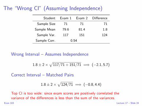
The “Wrong CI” (Assuming Independence)
Student Exam 1 Exam 2 Difference
Sample Size 71 71 71
Sample Mean 79.6 81.4 1.8
Sample Var. 117 151 124
Sample Corr. 0.54
Wrong Interval – Assumes Independence
1.8± 2×√117/71 + 151/71 =⇒ (−2.1, 5.7)
Correct Interval – Matched Pairs
1.8± 2×√
124/71 =⇒ (−0.8, 4.4)
Top CI is too wide: since exam scores are positively correlated thevariance of the differences is less than the sum of the variances.
Econ 103 Lecture 17 – Slide 24

CIs for a Difference of Means – Two Cases
Independent Samples
Two independent samples: X1, . . . ,Xn and Y1, . . . ,Ym.
Matched Pairs
Matched pairs (X1,Y1), . . . , (Xn,Yn) where Xi is not independent
of Yi but each pair (Xi ,Yi ) is independent of the other pairs.
Crucial Points
I Learn to recognize matched pairs and independent samples
setups since the CIs are different!
I Two equivalent ways to construct matched pairs CI:
1. Method 1: use sample mean and std. dev. of Di = Xi − Yi
2. Method 2: use Xn, Yn, along with SX , SY and rXY
Econ 103 Lecture 17 – Slide 25

Lecture #18 – Hypothesis Testing I
The Pepsi Challenge
Analogy between Hypothesis Testing and a Criminal Trial
Steps in a Hypothesis Test
Econ 103 Lecture 18 – Slide 1
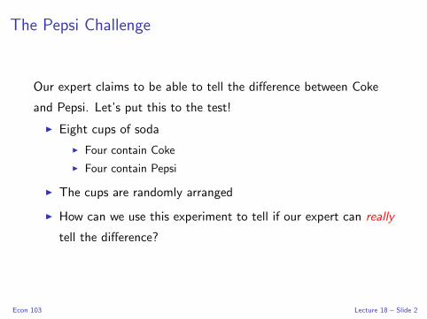
The Pepsi Challenge
Our expert claims to be able to tell the difference between Coke
and Pepsi. Let’s put this to the test!
I Eight cups of soda
I Four contain Coke
I Four contain Pepsi
I The cups are randomly arranged
I How can we use this experiment to tell if our expert can really
tell the difference?
Econ 103 Lecture 18 – Slide 2

The Results:
# of Cokes Correctly Identified:
What do you think? Can our expert really tell the difference?
(a) Yes
(b) No
Econ 103 Lecture 18 – Slide 3

If you just guess randomly, what is the probability of identifying all
four cups of Coke correctly?
I(84
)= 70 ways to choose four of the eight cups.
I If guessing randomly, each of these is equally likely
I Only one of the 70 possibilities corresponds to correctly
identifying all four cups of Coke.
I Thus, the probability is 1/70 ≈ 0.014
Econ 103 Lecture 18 – Slide 4

Probabilities if Guessing Randomly
# Correct 0 1 2 3 4
Prob. 1/70 16/70 36/70 16/70 1/70
Econ 103 Lecture 18 – Slide 5

# Correct 0 1 2 3 4
Prob. 1/70 16/70 36/70 16/70 1/70
If you’re just guessing, what is the probability of identifying at
least three Cokes correctly?
I Probabilities of mutually exclusive events sum.
I P(all four correct) = 1/70
I P(exactly 3 correct )= 16/70
I P(at least three correct) = 17/70 ≈ 0.24
Econ 103 Lecture 18 – Slide 6

The Pepsi Challenge
I Even if you’re just guessing randomly, the probability of
correctly identifying three or more Cokes is around 24%
I In contrast, the probability of identifying all four Cokes
correctly is only around 1.4% if you’re guessing randomly.
I We should probably require the expert to get them all right. . .
I What if the expert gets them all wrong? This also has
probability 1.4% if you’re guessing randomly. . .
That was a hypothesis test! We’ll go through the details in a
moment, but first an analogy. . .
Econ 103 Lecture 18 – Slide 7

Criminal Trial
I The person on trial is either innocent
or guilty (but not both!)
I “Innocent Until Proven Guilty”
I Only convict if evidence is “beyond a
reasonable doubt”
I Not Guilty rather than Innocent
I Acquit 6= Innocent
I Two Kinds of Errors:
I Convict the innocent
I Acquit the guilty
I Convicting the innocent is a worse
error. Want this to be rare even if it
means acquitting the guilty.
Hypothesis Testing
I Either the null hypothesis H0 or the
alternative H1 hypothesis is true.
I Assume H0 to start
I Only reject H0 in favor of H1 if there
is strong evidence.
I Fail to reject rather than Accept H0
I (Fail to reject H0) 6= (H0 True)
I Two Kinds of Errors:
I Reject true H0 (Type I)
I Don’t reject false H0 (Type II)
I Type I errors (reject true H0) are
worse: make them rare even if that
means more Type II errors.
Econ 103 Lecture 18 – Slide 8

How is the Pepsi Challenge a Hypothesis Test?
Null Hypothesis H0
Can’t tell the difference between Coke and Pepsi: just guessing.
Alternative Hypothesis H1
Able to tell which ones are Coke and which are Pepsi.
Type I Error – Reject H0 even though it’s true
Decide expert can tell the difference when she’s really just guessing.
Type II Error – Fail to reject H0 even though it’s false
Decide expert just guessing when she really can tell the difference.
Econ 103 Lecture 18 – Slide 9

How do we carry out a hypothesis test?
Step 1 – Specify H0 and H1
I Pepsi Challenge: H0 – our “expert” is guessing randomly
I Pepsi Challenge: H1 – our “expert” can tell which is Coke
Step 2 – Choose a Test Statistic Tn
I Tn uses sample data to measure the plausibility of H0 vs. H1
I Pepsi Challenge: Tn = Number of Cokes correctly identified
I Lots of Cokes correct ⇒ implausible that you’re just guessing
Econ 103 Lecture 18 – Slide 10

Step 3 – Calculate Distribution of Tn under H0
I Under the null = Under H0 = Assuming H0 is true
I To carry out our test, need sampling dist. of Tn under H0
I H0 must be “specific enough” that we can do the calculation.
I Pepsi Challenge:
# Correct 0 1 2 3 4
Prob. 1/70 16/70 36/70 16/70 1/70
Econ 103 Lecture 18 – Slide 11
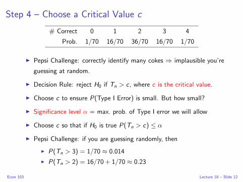
Step 4 – Choose a Critical Value c
# Correct 0 1 2 3 4
Prob. 1/70 16/70 36/70 16/70 1/70
I Pepsi Challenge: correctly identify many cokes ⇒ implausible you’re
guessing at random.
I Decision Rule: reject H0 if Tn > c , where c is the critical value.
I Choose c to ensure P(Type I Error) is small. But how small?
I Significance level α = max. prob. of Type I error we will allow
I Choose c so that if H0 is true P(Tn > c) ≤ α
I Pepsi Challenge: if you are guessing randomly, then
I P(Tn > 3) = 1/70 ≈ 0.014
I P(Tn > 2) = 16/70 + 1/70 ≈ 0.23
Econ 103 Lecture 18 – Slide 12

How do we carry out a hypothesis test?
# Correct 0 1 2 3 4
Prob. 1/70 16/70 36/70 16/70 1/70
Step 1 – Specify Null Hypothesis H0 and alternative Hypothesis H1
Step 2 – Choose Test Statistic Tn
Step 3 – Calculate sampling dist of Tn under H0
Step 4 – Choose Critical Value c
Step 5 – Look at the data: if Tn > c, reject H0.
Pepsi Challenge
If α = 0.05 we need c = 3 so that P(Tn > 3) ≤ α under H0.
Based on the results for our expert, would we reject H0?
Econ 103 Lecture 18 – Slide 13

Lecture #19 – Hypothesis Testing II
Test for the mean of a normal population (variance known)
Relationship Between Confidence Intervals and Hypothesis Tests
P-values
Econ 103 Lecture 19 – Slide 1

A Simple Example
Suppose X1, . . . ,X100 ∼ iid N(µ, σ2 = 9) and we want to test
H0 : µ = 2
H1 : µ 6= 2
Step 1 – Specify Null Hypothesis H0 and alternative Hypothesis H1 X
Step 2 – Choose Test Statistic Tn
If X is far from 2 then µ = 2 is implausible. Why?
Econ 103 Lecture 19 – Slide 2

Suppose X1, . . . ,X100 ∼ iid N(2, σ2 = 9). What is the sampling
distribution of X?
(a) N(0, 1)
(b) t(99)
(c) N(2, 0.3)
(d) N(2, 1)
(e) N(2, 0.09)
Econ 103 Lecture 19 – Slide 3

If Xn is far from 2, then µ = 2 is implausible
Since X1, . . . ,X100 ∼ iid N(µ, 9), if µ = 2 then X ∼ N(2, 0.09)
P(a ≤ X ≤ b) = P
(a− 2
3/10≤ X − 2
3/10≤ b − 2
3/10
)= P
(a− 2
0.3≤ Z ≤ b − 2
0.3
)where Z ∼ N(0, 1) so we see that if H0 : µ = 2 is true then
P(1.7 ≤ X ≤ 2.3) = P(−1 ≤ Z ≤ 1) ≈ 0.68
P(1.4 ≤ X ≤ 2.6) = P(−2 ≤ Z ≤ 2) ≈ 0.95
P(1.1 ≤ X ≤ 2.9) = P(−3 ≤ Z ≤ 3) > 0.99
Econ 103 Lecture 19 – Slide 4

Step 2 – Choose Test Statistic Tn
I Reject H0 : µ = 2 if the sample mean is far from 2.
I ⇒ Tn should depend on the distance from X to 2, i.e. |X − 2|.
I We can make our subsequent calculations much easier if we
choose a scale for Tn that is convenient under H0. . .
µ = 2 ⇒ X − 2 ∼ N(0, 0.09)
X − 2
0.3∼ N(0, 1)
So we will set Tn =
∣∣∣∣ X − 2
0.3
∣∣∣∣Econ 103 Lecture 19 – Slide 5

A Simple Example: X1, . . . ,X100 ∼ iid N(µ, σ2 = 9)
Step 1 – H0 : µ = 2, H1 : µ 6= 2 X
Step 2 – Tn =
∣∣∣∣ X − 2
0.3
∣∣∣∣ XStep 3 – If µ = 2 then
(X − 2
0.3
)∼ N(0, 1) X
Step 4 – Choose Critical Value c
(i) Specify significance level α.
(ii) Choose c so that P(Tn > c) = α under H0 : µ = 2.
Econ 103 Lecture 19 – Slide 6

Choose c so that P(Tn > c) = α under H0
Tn =
∣∣∣∣ X − 2
0.3
∣∣∣∣ and µ = 2 =⇒ X − 2
0.3∼ N(0, 1)
P
(∣∣∣∣ X − 2
0.3
∣∣∣∣ > c
)= α
1− P
(∣∣∣∣ X − 2
0.3
∣∣∣∣ ≤ c
)= α
P
(∣∣∣∣ X − 2
0.3
∣∣∣∣ ≤ c
)= 1− α
P
(−c ≤ X − 2
0.3≤ c
)= 1− α
Hence: c = qnorm(1− α/2) which should look familiar!
Econ 103 Lecture 19 – Slide 7

A Simple Example: X1, . . . ,X100 ∼ iid N(µ, σ2 = 9)
Step 1 – H0 : µ = 2, H1 : µ 6= 2 X
Step 2 – Tn =
∣∣∣∣ X − 2
0.3
∣∣∣∣ XStep 3 – If µ = 2 then
(X − 2
0.3
)∼ N(0, 1) X
Step 4 – c = qnorm(1− α/2) X
Step 5 – Look at the data: if Tn > c, reject H0
I Suppose I choose α = 0.05. Then c ≈ 2.
I I observe a sample of 100 observations. Suppose x = 1.34
Tn =
∣∣∣∣ x − 2
0.3
∣∣∣∣ = ∣∣∣∣1.34− 2
0.3
∣∣∣∣ = 2.2
I Since Tn > c , I reject H0 : µ = 2.
Econ 103 Lecture 19 – Slide 8

Reporting the Results of a Test
Our Example: X1, . . . ,X100 ∼ iid N(µ, 9)
I H0 : µ = 2 vs. H1 : µ 6= 2
I Tn = |(Xn − 2)/0.3|
I α = 0.05 =⇒ c ≈ 2
Suppose x = 1.34
Then Tn = 2.2. Since this is greater than c for α = 0.05, we reject
H0 : µ = 2 at the 5% significance level.
Suppose instead that x = 1.82
Then Tn = 0.6. Since this is less than c for α = 0.05, we fail to
reject H0 : µ = 2 at the 5% signifcance level.
Econ 103 Lecture 19 – Slide 9

General Version of Preceding Example
X1, . . . ,Xn ∼ iid N(µ, σ2) with σ2 known and we want to test:
H0 : µ = µ0
H1 : µ 6= µ0
where µ0 is some specified value for the population mean.
I |Xn − µ0| tells how far sample mean is from µ0.
I Reject H0 : µ = µ0 if sample mean is far from µ0.
I Under H0 : µ = µ0,Xn − µ0
σ/√n
∼ N(0, 1).
I Test statistic Tn =
∣∣∣∣ Xn − µ0
σ/√n
∣∣∣∣I Reject H0 : µ = µ0 if Tn > qnorm(1− α/2)
Econ 103 Lecture 19 – Slide 10

Suppose X1, . . . ,X64 ∼ iid N(µ, σ2 = 25) and we want to test
H0 : µ = 0 vs. H1 : µ 6= 0 with α = 0.32. If we observe x = 0.5
what is our decision?
(a) Reject H0
(b) Fail to Reject H0
(c) Not enough information to determine.
Tn =∣∣∣0.5−0
5/8
∣∣∣ = 0.5× 8/5 = 0.8, qnorm(1− 0.32/2) ≈ 1
Fail to reject H0
Econ 103 Lecture 19 – Slide 11

What is this test telling us to do?
Return to the example where H0 : µ = 2 vs. H1 : µ 6= 2 and
X1, . . . ,X100 ∼ iid N(µ, 9) with α = 0.05:
Reject H0 if
∣∣∣∣ Xn − 2
0.3
∣∣∣∣ > 2
Reject H0 if |Xn − 2| > 0.6
Reject H0 if (Xn < 1.4) or (Xn > 2.6)
Reject H0 : µ = 2 if Xn is far from 2. How far? Depends on choice
of α along with sample size and population variance.
Econ 103 Lecture 19 – Slide 12
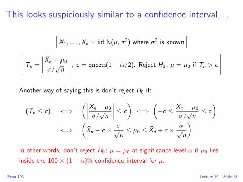
This looks suspiciously similar to a confidence interval. . .
X1, . . . ,Xn ∼ iid N(µ, σ2) where σ2 is known
Tn =
∣∣∣∣ Xn − µ0
σ/√n
∣∣∣∣ , c = qnorm(1− α/2), Reject H0 : µ = µ0 if Tn > c
Another way of saying this is don’t reject H0 if:
(Tn ≤ c) ⇐⇒(∣∣∣∣ Xn − µ0
σ/√n
∣∣∣∣ ≤ c
)⇐⇒
(−c ≤ Xn − µ0
σ/√n
≤ c
)⇐⇒
(Xn − c × σ√
n≤ µ0 ≤ Xn + c × σ√
n
)In other words, don’t reject H0 : µ = µ0 at significance level α if µ0 lies
inside the 100× (1− α)% confidence interval for µ.
Econ 103 Lecture 19 – Slide 13

CIs and Hypothesis Tests are Intimately Related
Our Simple Example
X1, . . . ,X100 ∼ iid N(µ, σ2 = 9) and observe x = 1.34
Test H0 : µ = 2 vs. H1 : µ 6= 2 with α = 0.05
Tn = 2.2, c = qnorm(1− 0.05/2) ≈ 2. Since Tn > c we reject.
95% Confidence Interval for µ
1.34± 2× 3/10 i.e. 1.34± 0.6 or equivalently (0.74, 1.94)
Another way to carry out the test. . .
Since 2 lies outside the 95% confidence interval for µ, if our
significance level is α = 0.05 we reject H0 : µ = 2.
Econ 103 Lecture 19 – Slide 14

X1, . . .X100 ∼ iid N(µX , 9) and Y1, . . . ,Y100 ∼ iid N(µY , 9)
Two researchers: H0 : µ = 2 vs. H1 : µ 6= 2 with α = 0.05
Researcher 1
I x = 1.34
I Tn = 2.2 > 2
I Reject H0 : µX = 2
Researcher 2
I y = 11.3
I Tn = 31 > 2
I Reject H0 : µY = 2
Both researchers would report “reject H0 at the 5% level” but
Researcher 2 found much stronger evidence against H0. . .
Econ 103 Lecture 19 – Slide 15

What if we had chosen a different significance level α?
Tn = 2.2, c = qnorm(1− α/2), Reject H0 : µ = 2 if Tn > c
α = 0.32 ⇒ c = qnorm(1− 0.32/2) ≈ 0.99 Reject
α = 0.10 ⇒ c = qnorm(1− 0.10/2) ≈ 1.64 Reject
α = 0.05 ⇒ c = qnorm(1− 0.05/2) ≈ 1.96 Reject
α = 0.04 ⇒ c = qnorm(1− 0.04/2) ≈ 2.05 Reject
α = 0.03 ⇒ c = qnorm(1− 0.03/2) ≈ 2.17 Reject
α = 0.02 ⇒ c = qnorm(1− 0.02/2) ≈ 2.33 Fail to Reject
α = 0.01 ⇒ c = qnorm(1− 0.01/2) ≈ 2.58 Fail to Reject
Econ 103 Lecture 19 – Slide 16

Result of Test Depends on Choice of α!
α = 0.32 ⇒ Reject
α = 0.10 ⇒ Reject
α = 0.05 ⇒ Reject
α = 0.04 ⇒ Reject
α = 0.03 ⇒ Reject
α = 0.02 ⇒ Fail to Reject
α = 0.01 ⇒ Fail to Reject
I If you reject H0 at a given choice
of α, you would also have rejected
at any larger choice of α.
I If you fail to reject H0 at a given
choice of α, you would also have
failed to reject at any smaller
choice of α.
Question
If α is large enough we will reject; if α is small enough, we won’t.
Where is the dividing line between reject and fail to reject?
Econ 103 Lecture 19 – Slide 17

P-Value: Dividing Line Between Reject and Fail to Reject
Tn = 2.2, c = qnorm(1− α/2), Reject H0 : µ = 2 if Tn > c
Question
Given that we observed a test statistic of 2.2, what choice of α
would put us just at the cusp of rejecting H0?
Answer
Whichever α makes c = 2.2! At this α we just barely fail to reject.
Econ 103 Lecture 19 – Slide 18

Calculating the P-value
Definition of a P-value
Significance level α such that the critical value c exactly equals the
observed value of the test statistic. Equivalently: α that lies
exactly on boundary between Reject and Fail to Reject.
Our Example
The observed value of the test statistic is 2.2 and the critical value
is qnorm(1− α/2), so we need to solve:
2.2 = qnorm(1− α/2)
pnorm(2.2) = pnorm (qnorm (1− α/2))
pnorm(2.2) = 1− α/2
α = 2× [1− pnorm(2.2)] ≈ 0.028
Econ 103 Lecture 19 – Slide 19

How to use a p-value?
Alternative to Steps 4–5
Rather than choosing α, computing critical value c and reporting
“Reject” or “Fail to Reject” at 100× α% level, just report p-value.
Example From Previous Slide
P-value for our test of H0 : µ = 2 against H1 : µ 6= 2 was ≈ 0.028
Using P-value to Test H0
Using the p-value we can test H0 for any α without doing any new
calculations! For p-value < α reject; for p-value ≥ α fail to reject.
Strength of Evidence Against H0
P-value measures strength of evidence against the null. Smaller p-value
= stronger evidence against H0. P-value does not measure size of effect.
Econ 103 Lecture 19 – Slide 20

Lecture #20 – Hypothesis Testing III
One-Sided Tests
Two-Sample Test For Difference of Means
Matched Pairs Test for Difference of Means
Econ 103 Lecture 20 – Slide 1
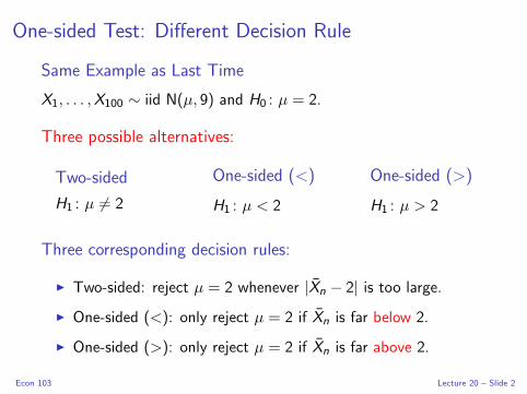
One-sided Test: Different Decision Rule
Same Example as Last Time
X1, . . . ,X100 ∼ iid N(µ, 9) and H0 : µ = 2.
Three possible alternatives:
Two-sided
H1 : µ 6= 2
One-sided (<)
H1 : µ < 2
One-sided (>)
H1 : µ > 2
Three corresponding decision rules:
I Two-sided: reject µ = 2 whenever |Xn − 2| is too large.
I One-sided (<): only reject µ = 2 if Xn is far below 2.
I One-sided (>): only reject µ = 2 if Xn is far above 2.
Econ 103 Lecture 20 – Slide 2

One-sided (>) Example: X1, . . . ,X100 ∼ iid N(µ, 9)
Null and Alternative
Test H0 : µ = 2 against H0 : µ > 2 with α = 0.05.
Test Statistic
Drop absolute value for one-sided test: Tn =Xn − 2
0.3
Decision Rule
Reject H0 : µ = 2 if test statistic is large and positive: Tn > c
Critical Value
Choose c so that P(type I error) = P(Tn > c |µ = 2) = 0.05
Under H0, Tn ∼ N(0, 1)
If Z ∼ N(0, 1) what value of c ensures P(Z > c) = 0.05?
Econ 103 Lecture 20 – Slide 3
One-sided (<) Example: X1, . . . ,X100 ∼ iid N(µ, 9)
Null and Alternative
Test H0 : µ = 2 against H1 : µ < 2 with α = 0.05.
Test Statistic
Drop absolute value for one-sided test: Tn =Xn − 2
0.3
Decision Rule
Reject H0 : µ = 2 if test statistic is large and negative: Tn < c
Critical Value
Choose c so that P(type I error) = P(Tn < c |µ = 2) = 0.05
Under H0, Tn ∼ N(0, 1)
If Z ∼ N(0, 1) what value of c ensures P(Z < c) = 0.05?
Econ 103 Lecture 20 – Slide 4

Critical Values – Two-sided vs. One-sided Tests: α = 0.05
−4 −2 0 2 4
0.0
0.1
0.2
0.3
0.4
Two−Sided Test
x
dnor
m(x
)
2.5%2.5%
−4 −2 0 2 40.
00.
10.
20.
30.
4
One−Sided Test (<)
x
dnor
m(x
)
5%
−4 −2 0 2 4
0.0
0.1
0.2
0.3
0.4
One−Sided Test (>)
x
dnor
m(x
)
5%
Two-Sided
Splits α = 0.05 between two tails: c = qnorm(1− 0.05/2) ≈ 1.96
One-Sided
One tail: c = qnorm(0.05) ≈ −1.64 for (<); qnorm(0.95) ≈ 1.64 for (>)
Econ 103 Lecture 20 – Slide 5

Example: X1, . . . ,X100 ∼ iid N(µ, 9), α = 0.05
Suppose x = 1.5 =⇒ (x − 2)/0.3 ≈ −1.67
Two-sided
H1 : µ 6= 2
Reject if |Tn| > 1.96
Tn = 1.67
Fail to reject
One-sided (<)
H1 : µ < 2
Reject if Tn < −1.64
Tn = −1.67
Reject
One-sided (>)
H1 : µ > 2
Reject if Tn > 1.64
Tn = −1.67
Fail to reject
I If One-sided (<) rejects, then one-sided (>) doesn’t and vice-versa.
I Two-sided and one-sided sometimes agree but sometimes disagree.
I One-sided test is “less stringent.”
Econ 103 Lecture 20 – Slide 6

Testing H0 : µ = µ0 when X1, . . . ,Xn ∼ iid N(µ, σ2)
Two-Sided
Reject H0 whenever
∣∣∣∣ Xn − µ0
σ/√n
∣∣∣∣ > qnorm(1− α/2)
One-Sided (<)
Reject H0 wheneverXn − µ0
σ/√n
< qnorm(α)
One-Sided (>)
Reject H0 wheneverXn − µ0
σ/√n
> qnorm(1− α)
Econ 103 Lecture 20 – Slide 7

One-sided P-value
I Only makes sense to calculate one-sided p-value when sign of test
stat. agrees with alternative:
I Preceding example: Tn = −1.67
I Calculate p-value for test vs. H1 : µ < 2 but not H1 : µ > 2
I Just as in two-sided test, p-value equals value of α for which c
exactly equals the observed test statistic:
I c = qnorm(α) for (<)
I c = qnorm(1− α) for (>)
I Example: −1.67 = qnorm(α) ⇐⇒ α = 0.047
I Use and report one-sided p-value in same way as two-sided p-value
Econ 103 Lecture 20 – Slide 8

Comparing One-sided and Two-sided Tests
I Two-sided test is the default.
I Don’t use one-sided unless you have a good reason!
I Relationship between CI and test only holds for two-sided.
I Why and when should we consider a one-sided test?
I Suppose we know a priori that µ < 2 is crazy/uninteresting
I Test of H0 : µ = 2 against H1 : µ > 2 with significance level α
has lower type II error rate than test against H1 : µ 6= 2.
I If you use a one-sided test you must choose (>) or (<) before
looking at the data. Otherwise the results are invalid.
Econ 103 Lecture 20 – Slide 9
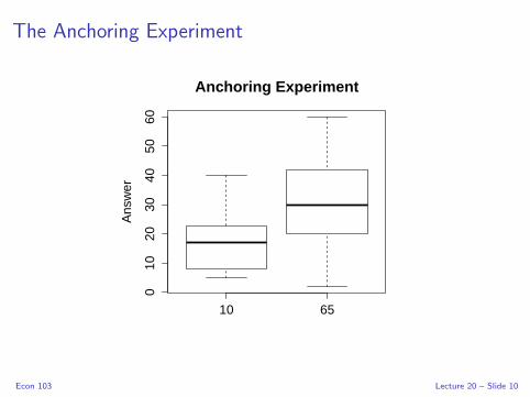
The Anchoring Experiment
10 65
010
2030
4050
60
Anchoring Experiment
Ans
wer
Econ 103 Lecture 20 – Slide 10

The Anchoring Experiment
Shown a “random” number and then asked what proportion of UN
member states are located in Africa.
“Hi” Group – Shown 65 (nHi = 46)
Sample Mean: 30.7, Sample Variance: 253
“Lo” Group – Shown 10 (nLo = 43)
Sample Mean: 17.1, Sample Variance: 86
Proceed via the CLT...
Econ 103 Lecture 20 – Slide 11
In words, what is our null hypothesis?
(a) There is a positive anchoring effect: seeing a higher random
number makes people report a higher answer.
(b) There is a negative anchoring effect: seeing a lower random
number makes people report a lower answer.
(c) There is an anchoring effect: it could be positive or negative.
(d) There is no anchoring effect: people aren’t influenced by
seeing a random number before answering.
Econ 103 Lecture 20 – Slide 12
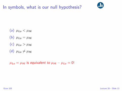
In symbols, what is our null hypothesis?
(a) µLo < µHi
(b) µLo = µHi
(c) µLo > µHi
(d) µLo 6= µHi
µLo = µHi is equivalent to µHi − µLo = 0!
Econ 103 Lecture 20 – Slide 13
Anchoring Experiment
Under the null, what should we expect to be true about the values
taken on by XLo and XHi?
(a) They should be similar in value.
(b) XLo should be the smaller of the two.
(c) XHi should be the smaller of the two.
(d) They should be different. We don’t know which will be larger.
Econ 103 Lecture 20 – Slide 14
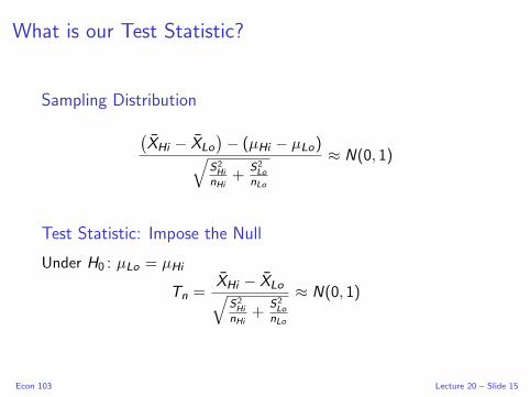
What is our Test Statistic?
Sampling Distribution
(XHi − XLo
)− (µHi − µLo)√
S2Hi
nHi+
S2Lo
nLo
≈ N(0, 1)
Test Statistic: Impose the Null
Under H0 : µLo = µHi
Tn =XHi − XLo√
S2Hi
nHi+
S2Lo
nLo
≈ N(0, 1)
Econ 103 Lecture 20 – Slide 15

What is our Test Statistic?XHi = 30.7, s2Hi = 253, nHi = 46
XLo = 17.1, s2Lo = 86, nLo = 43
Under H0 : µLo = µHi
Tn =XHi − XLo√
S2Hi
nHi+
S2Lo
nLo
≈ N(0, 1)
Plugging in Our Data
Tn =XHi − XLo√
S2Hi
nHi+
S2Lo
nLo
≈ 5
Econ 103 Lecture 20 – Slide 16

Anchoring Experiment Example
Approximately what critical value should we use to test
H0 : µLo = µHi against the two-sided alternative at the 5%
significance level?
α 0.10 0.05 0.01
qnorm(1− α) 1.28 1.64 2.33
qnorm(1− α/2) 1.64 1.96 2.58
... Approximately 2
Econ 103 Lecture 20 – Slide 17

Anchoring Experiment Example
Which of these commands would give us the p-value of our test of
H0 : µLo = µHi against H1 : µLo < µHi at significance level α?
(a) qnorm(1− α)
(b) qnorm(1− α/2)
(c) 1 - pnorm(5)
(d) 2 * (1 - pnorm(5))
Econ 103 Lecture 20 – Slide 18
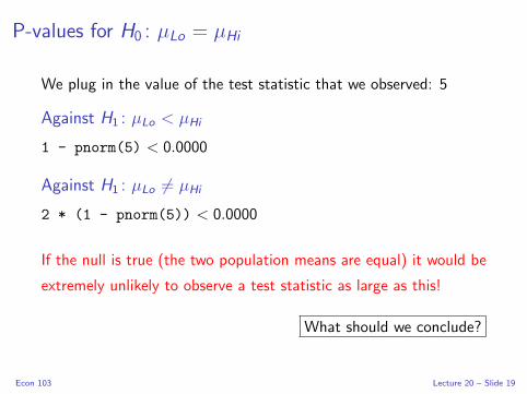
P-values for H0 : µLo = µHi
We plug in the value of the test statistic that we observed: 5
Against H1 : µLo < µHi
1 - pnorm(5) < 0.0000
Against H1 : µLo 6= µHi
2 * (1 - pnorm(5)) < 0.0000
If the null is true (the two population means are equal) it would be
extremely unlikely to observe a test statistic as large as this!
What should we conclude?
Econ 103 Lecture 20 – Slide 19

Which Exam is Harder?
Student Exam 1 Exam 2 Difference
1 57.1 60.7 3.6...
......
...
71 78.6 82.9 4.3
Sample Mean: 79.6 81.4 1.8
Sample Var. 117 151 124
Sample Corr. 0.54
Again, we’ll use the CLT.
Econ 103 Lecture 20 – Slide 20

One-Sample Hypothesis Test Using Differences
Let Di = Xi − Yi be (Midterm 2 Score - Midterm 1 Score) for student i
Null Hypothesis
H0 : µ1 = µ2, i.e. both exams were of the same difficulty
Two-Sided Alternative
H1 : µ1 6= µ2, i.e. one exam was harder than the other
One-Sided Alternative
H1 : µ2 > µ1, i.e. the second exam was easier
Econ 103 Lecture 20 – Slide 21

Decision Rules
Let Di = Xi − Yi be (Midterm 2 Score - Midterm 1 Score) for student i
Test Statistic
Dn
SE (Dn)=
1.8√124/71
≈ 1.36
Two-Sided Alternative
Reject H0 : µ1 = µ2 in favor of H1 : µ1 6= µ2 if |Dn| is sufficiently large.
One-Sided Alternative
Reject H0 : µ1 = µ2 in favor of H1 : µ2 > µ1 if Dn is sufficiently large.
Econ 103 Lecture 20 – Slide 22

Reject against Two-sided Alternative with α = 0.1?
Dn
SE (Dn)=
1.8√124/71
≈ 1.36
α 0.10 0.05 0.01
qnorm(1− α) 1.28 1.64 2.33
qnorm(1− α/2) 1.64 1.96 2.58
(a) Reject
(b) Fail to Reject
(c) Not Sure
Econ 103 Lecture 20 – Slide 23

Reject against One-sided Alternative with α = 0.1?
Dn
SE (Dn)=
1.8√124/71
≈ 1.36
α 0.10 0.05 0.01
qnorm(1− α) 1.28 1.64 2.33
qnorm(1− α/2) 1.64 1.96 2.58
(a) Reject
(b) Fail to Reject
(c) Not Sure
Econ 103 Lecture 20 – Slide 24
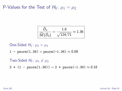
P-Values for the Test of H0 : µ1 = µ2
Dn
SE (Dn)=
1.8√124/71
≈ 1.36
One-Sided H1 : µ2 > µ1
1 - pnorm(1.36) = pnorm(-1.36) ≈ 0.09
Two-Sided H1 : µ1 6= µ2
2 * (1 - pnorm(1.36)) = 2 * pnorm(-1.36) ≈ 0.18
Econ 103 Lecture 20 – Slide 25

Lecture #21 – Testing/CI Roundup
One-sample Test for Proportion
Test for Difference of Proportions
Statistical vs. Practical Significance
Data-Dredging
Econ 103 Lecture 21 – Slide 1

Tests for Proportions
Basic Idea
The population can’t be normal (it’s Bernoulli) so we use the CLT
to get approximate sampling distributions (c.f. Lecture 18).
But there’s a small twist!
Bernoulli RV only has a single unknown parameter =⇒ we know
more about the population under H0 in a proportions problem than
in the other testing examples we’ve examined...
Econ 103 Lecture 21 – Slide 2

Tests for Proportions: One-Sample Example
From Pew Polling Data
54% of a random sample of 771 registered voters correctly
identified 2012 presidential candidate Mitt Romney as Pro-Life.
Sampling Model
X1, . . . ,Xn ∼ iid Bernoulli(p)
Sample Statistic
Sample Proportion: p =1
n
n∑i=1
Xi
Suppose I wanted to test H0 : p = 0.5
Econ 103 Lecture 21 – Slide 3

Tests for Proportions: One Sample Example
Under H0 : p = 0.5 what is the standard error of p?
(a) 1
(b)√
p(1− p)/n
(c) σ/√n
(d) 1/(2√n)
(e) p(1− p)
p = 0.5 =⇒√
0.5(1− 0.5)/n = 1/(2√n)
Under the null we know the SE! Don’t have to estimate it!
Econ 103 Lecture 21 – Slide 4

One-Sample Test for a Population Proportion
Sampling Model
X1, . . . ,Xn ∼ iid Bernoulli(p)
Null Hypothesis
H0 : p = Known Constant p0
Test Statistic
Tn =p − p0√
p0(1− p0)/n≈ N(0, 1) under H0 provided n is large
Econ 103 Lecture 21 – Slide 5

One-Sample Example H0 : p = 0.5
54% of a random sample of 771 registered voters knew Mitt Romney is Pro-Life.
Tn =p − p0√p0(1− p0)
n
= 2√771(0.54− 0.5)
= 0.08×√771 ≈ 2.2
One-Sided p-value
1 - pnorm(2.2) ≈ 0.014
Two-Sided p-value
2 * (1 - pnorm(2.2)) ≈ 0.028
Econ 103 Lecture 21 – Slide 6

Tests for Proportions: Two-Sample Example
From Pew Polling Data
53% of a random sample of 238 Democrats correctly identified
Mitt Romney as Pro-Life versus 61% of 239 Republicans.
Sampling Model
Republicans: X1, . . . ,Xn ∼ iid Bernoulli(p) independent of
Democrats: Y1, . . . ,Ym ∼ iid Bernoulli(q)
Sample Statistics
Sample Proportions: p =1
n
n∑i=1
Xi , q =1
m
m∑i=1
Yi
Suppose I wanted to test H0 : p = q
Econ 103 Lecture 21 – Slide 7

A More Efficient Estimator of the SE Under H0
Don’t Forget!
Standard Error (SE) means “std. dev. of sampling distribution” so
you should know how to prove that that:
SE (p − q) =
√p(1− p)
n+
q(1− q)
m
Under H0 : p = q
Don’t know values of p and q: only that they are equal.
Econ 103 Lecture 21 – Slide 8

A More Efficient Estimator of the SE Under H0
One Possible Estimate
SE =
√p(1− p)
n+
q(1− q)
m
A Better Estimate Under H0
SEPooled =
√π(1− π)
(1
n+
1
m
)where π =
np +mq
n +m
Why Pool?
If p = q, the two populations are the same. This means we can get
a more precise estimate of the common population proportion by
pooling. More data = Lower Variance =⇒ better estimated SE.
Econ 103 Lecture 21 – Slide 9

Two-Sample Test for Proportions
Sampling Model
X1, . . . ,Xn ∼ iid Bernoulli(p) indep. of Y1, . . . ,Ym ∼ iid Bernoulli(q)
Sample Statistics
Sample Proportions: p =1
n
n∑i=1
Xi , q =1
m
m∑i=1
Yi
Null Hypothesis
H0 : p = q ⇐ i.e. p − q = 0
Pooled Estimator of SE under H0
π =np +mq
n +m, SEPooled =
√π(1− π) (1/n + 1/m)
Test Statistic
Tn =p − q
SEPooled
≈ N(0, 1) under H0 provided n and m are large
Econ 103 Lecture 21 – Slide 10

Two-Sample Example H0 : p = q
53% of 238 Democrats knew Romney is Pro-Life vs. 61% of 239 Republicans
π =np +mq
n +m=
239× 0.61 + 238× 0.53
239 + 238≈ 0.57
SEPooled =√π(1− π) (1/n + 1/m) =
√0.57× 0.43(1/239 + 1/238)
≈ 0.045
Tn =p − q
SEPooled
=0.61− 0.53
0.045≈ 1.78
One-Sided P-Value
1 - pnorm(1.78)≈ 0.04
Two-Sided P-Value
2 * (1 - pnorm(1.78))≈ 0.08
Econ 103 Lecture 21 – Slide 11

Terminology I Have Intentionally Avoided Until Now
Statistical Significance
Suppose we carry out a hypothesis test at the α% level and, based
on our data, reject the null. You will often see this situation
described as “statistical significance.”
In Other Words...
When people say “statistically significant” what they really mean is
that they rejected the null hypothesis.
Econ 103 Lecture 21 – Slide 12

Some Examples
I We found a difference between the “Hi” and “Lo” groups in
the anchoring experiment that was statistically significant at
the 5% level based on data from a past semester.
I Our 95% CI for the proportion of US voters who know who
John Roberts did not include 0.5. Viewed as a two-sided test,
we found that the difference between the true population
proportion and 0.5 was statistically significant at the 5% level.
Econ 103 Lecture 21 – Slide 13
Why Did I Avoid this Terminology?
Statistical Significance 6= Practical Importance
I You need to understand the term “statistically significant” since it is
widely used. A better term for the idea, however, would be
“statistically discernible”
I Unfortunately, many people are confuse “significance” in the
narrow, technical sense with the everyday English word meaning
“important”
I Statistically Significant Does Not Mean Important!”
I A difference can be practically unimportant but statistically
significant.
I A difference can be practically important but statistically
insignificant.
Econ 103 Lecture 21 – Slide 14

P-value Measures Strength of
Evidence Against H0
Not The Size of an Effect!
Econ 103 Lecture 21 – Slide 15

Statistically Significant but Not Practically Important
I flipped a coin 10 million times (in R) and got 4990615 heads.
Test of H0 : p = 0.5 against H1 : p 6= 0.5
T =p − 0.5√
0.5(1− 0.5)/n≈ −5.9 =⇒ p-value ≈ 0.000000003
Approximate 95% Confidence Interval
p ± qnorm(1− 0.05/2)
√p(1− p)
n=⇒ (0.4988, 0.4994)
(Such a huge sample size that refined vs. textbook CI makes no difference)
Actual p was 0.499
Econ 103 Lecture 21 – Slide 16

Practically Important But Not Statistically Significant
Vickers: “What is a P-value Anyway?” (p. 62)
Just before I started writing this book, a study was published
reporting about a 10% lower rate of breast cancer in women who
were advised to eat less fat. If this indeed the true difference, low
fat diets could reduce the incidence of breast cancer by tens of
thousands of women each year – astonishing health benefit for
something as simple and inexpensive as cutting down on fatty
foods. The p-value for the difference in cancer rates was 0.07 and
here is the key point: this was widely misinterpreted as indicating
that low fat diets don’t work. For example, the New York Times
editorial page trumpeted that “low fat diets flub a test” and
claimed that the study provided “strong evidence that the war
against all fats was mostly in vain.” However failure to prove that a
treatment is effective is not the same as proving it ineffective.
Econ 103 Lecture 21 – Slide 17

Do Students with 4-Letter Surnames Do Better?Based on Data from Midterm 1 Last Semester
4-Letter Surname
x = 88.9
sx = 10.4
nx = 12
Other Surnames
y = 74.4
sy = 20.7
ny = 92
Difference of Means
x − y = 14.5
Standard Error
SE =√s2x /nx + s2y /ny ≈ 3.7
Test Statistic
T = 14.5/3.7 ≈ 3.9
Econ 103 Lecture 21 – Slide 18
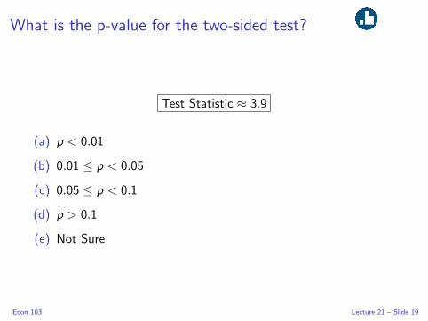
What is the p-value for the two-sided test?
Test Statistic ≈ 3.9
(a) p < 0.01
(b) 0.01 ≤ p < 0.05
(c) 0.05 ≤ p < 0.1
(d) p > 0.1
(e) Not Sure
Econ 103 Lecture 21 – Slide 19

What do these results mean?
Evaulate this statement in light of our hypothesis test:
Students with four-letter long surnames do better, on
average, on the first midterm of Econ 103 at UPenn.
(a) Strong evidence in favor
(b) Moderate evidence in favor
(c) No evidence either way
(d) Moderate evidence against
(e) Strong evidence against
Econ 103 Lecture 21 – Slide 20

I just did 134 Hypothesis Tests...
... and 11 of them were significant at the 5% level.
group sign p.value x.bar N.x s.x y.bar N.y s.y
26 first1 = P 1 0.000 93.8 3 2.9 75.5 101 20.4
70 id2 = 7 1 0.000 94.6 5 3.3 75.1 99 20.4
134 id8 = 0 1 0.000 92.6 7 4.9 74.8 97 20.5
5 Nlast = 4 1 0.001 88.9 12 10.4 74.4 92 20.7
90 id4 = 8 1 0.003 87.7 9 9.0 74.9 95 20.7
105 id6 = 8 1 0.003 88.1 5 5.8 75.4 99 20.6
109 id6 = 2 1 0.007 88.9 8 10.7 75.0 96 20.6
9 Nlast = 2 1 0.016 90.4 5 9.3 75.3 99 20.5
49 last1 = P -1 0.036 65.2 6 9.9 76.7 98 20.6
65 id2 = 1 1 0.038 84.3 9 10.1 75.3 95 20.9
117 id7 = 8 1 0.041 83.4 13 11.6 75.0 91 21.1
Econ 103 Lecture 21 – Slide 21

Data-Dredging
I Suppose you have a long list of null hypotheses and assume,
for the sake of argument that all of them are true.
I E.g. there’s no difference in grades between students with
different 4th digits of their student id number.
I We’ll still reject about 5% of the null hypotheses.
I Academic journals tend only to publish results in which a null
hypothesis is rejected at the 5% level or lower.
I We end up with the bizarre result that “most published
studies are false.”
I posted a reading about this on Piazza: “The Economist - Trouble
in the Lab.” To learn even more, see Ioannidis (2005)
Econ 103 Lecture 21 – Slide 22

Green Jelly Beans Cause Acne!xkcd #882
Figure: Go and read this comic strip: before today’s lecture you wouldn’t
have gotten the joke!
Econ 103 Lecture 21 – Slide 23

Lecture #22 – Regression II
The Population Regression Model
Inference for Regression
Example: Height and Handspan
Multiple Regression
Residual Standard Deviation and R2
Econ 103 Lecture 22 – Slide 1

Beyond Regression as a Data Summary
Based on a sample of Econ 103 students, we made the following graph of
handspan against height, and fitted a linear regression:
18 20 22 24 26
60
65
70
75
Handspan (cm)
He
igh
t (in
)
The estimated slope was about 1.4 inches/cm and the estimated
intercept was about 40 inches.
What if anything does this tell us about the relationship between height
and handspan in the population?
Econ 103 Lecture 22 – Slide 2
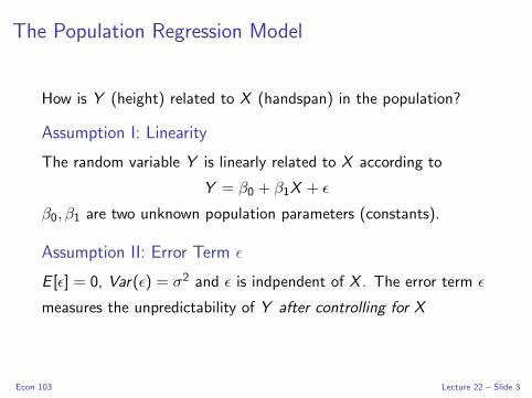
The Population Regression Model
How is Y (height) related to X (handspan) in the population?
Assumption I: Linearity
The random variable Y is linearly related to X according to
Y = β0 + β1X + ε
β0, β1 are two unknown population parameters (constants).
Assumption II: Error Term ε
E [ε] = 0, Var(ε) = σ2 and ε is indpendent of X . The error term ε
measures the unpredictability of Y after controlling for X
Econ 103 Lecture 22 – Slide 3

Predictive Interpretation of Regression
Under Assumptions I and II
E [Y |X ] = β0 + β1X
I “Best guess” of Y having observed X = x is β0 + β1x
I If X = 0, we predict Y = β0
I If two people differ by one unit in X , we predict that they will
differ by β1 units in Y .
The only problem is, we don’t know β0, β1...
Econ 103 Lecture 22 – Slide 4
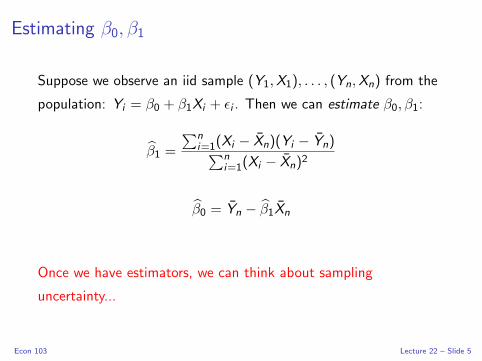
Estimating β0, β1
Suppose we observe an iid sample (Y1,X1), . . . , (Yn,Xn) from the
population: Yi = β0 + β1Xi + εi . Then we can estimate β0, β1:
β1 =
∑ni=1(Xi − Xn)(Yi − Yn)∑n
i=1(Xi − Xn)2
β0 = Yn − β1Xn
Once we have estimators, we can think about sampling
uncertainty...
Econ 103 Lecture 22 – Slide 5

Sampling Uncertainty: Pretend the Class is our Population
18 20 22 24 26
60
65
70
75
Handspan (cm)
He
igh
t (in
)
Figure: Estimated Slope = 1.4, Estimated Intercept = 40
Econ 103 Lecture 22 – Slide 6

Sampling Distribution of Regression Coefficients β0 and β1
Choose 25 Students from Class List with Replacement
��
���
Sample 1
?
β(1)0 , β
(1)1
?
Sample 2
?
β(2)0 , β
(2)1
...
...
@@
@@@R
Sample 1000
?
β(1000)0 , β
(1000)1
Repeat 1000 times → get 1000 different pairs of estimates
Sampling Distribution: long-run relative frequencies
Econ 103 Lecture 22 – Slide 7
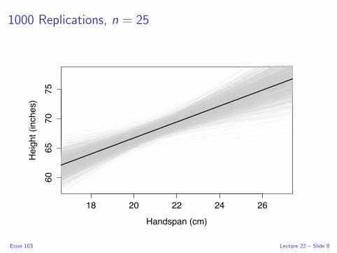
1000 Replications, n = 25
18 20 22 24 26
60
65
70
75
Handspan (cm)
He
igh
t (in
ch
es)
Econ 103 Lecture 22 – Slide 8

Population: Intercept = 40, Slope = 1.4
Intercept EstimatesFrequency
20 40 60
050
150
250
Slope Estimates
Frequency
0.5 1.5 2.50
50
100
150
200
250
Based on 1000 Replications, n = 25Econ 103 Lecture 22 – Slide 9

Inference for Linear Regression
Central Limit Theorem
β − β
SE (β)≈ N(0, 1)
How to calculate SE?
I Complicated
I Depends on variance of errors ε and all predictors in regression.
I We’ll look at a few simple examples
I R does this calculation for us
I Requires assumptions about population errors εi
I Simplest (and R default) is to assume εi ∼ iid(0, σ2)
I Weaker assumptions in Econ 104Econ 103 Lecture 22 – Slide 10

Intuition for What Effects SE (β1) for Simple Regression
SE (β1) ≈σ√n· 1
sX
I σ = SD(ε) – inherent variability of the Y , even after
controlling for X
I n is the sample size
I sX is the sampling variability of the X observations.
Econ 103 Lecture 22 – Slide 11

I treated the class as our population for the purposes of the
simulation experiment but it makes more sense to think of the
class as a sample from some population. We’ll take this
perspective now and think about various inferences we can draw
from the height and handspan data using regression.
Econ 103 Lecture 22 – Slide 12
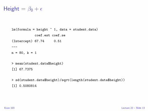
Height = β0 + ε
lm(formula = height ~ 1, data = student.data)
coef.est coef.se
(Intercept) 67.74 0.51
---
n = 80, k = 1
> mean(student.data$height)
[1] 67.7375
> sd(student.data$height)/sqrt(length(student.data$height))
[1] 0.5080814
Econ 103 Lecture 22 – Slide 13

Dummy Variable (aka Binary Variable)
A predictor variable that takes on only two values: 0 or 1. Used to
represent two categories, e.g. Male/Female.
Econ 103 Lecture 22 – Slide 14

Height = β0 + β1 Male +ε
lm(formula = height ~ sex, data = student.data)
coef.est coef.se
(Intercept) 64.46 0.56
sexMale 6.10 0.76
---
n = 80, k = 2
residual sd = 3.38, R-Squared = 0.45
> mean(male$height) - mean(female$height)
[1] 6.09868
> sqrt(var(male$height)/length(male$height) +
var(female$height)/length(female$height))
[1] 0.7463796
Econ 103 Lecture 22 – Slide 15

Height = β0 + β1 Male +ε
What is the ME for an approximate 95% confidence interval for
the difference of population means of height: (men - women)?
lm(formula = height ~ sex, data = student.data)
coef.est coef.se
(Intercept) 64.46 0.56
sexMale 6.10 0.76
---
n = 80, k = 2
residual sd = 3.38, R-Squared = 0.45
Econ 103 Lecture 22 – Slide 16

Height = β0 + β1 Handspan +ε
lm(formula = height ~ handspan, data = student.data)
coef.est coef.se
(Intercept) 39.60 3.96
handspan 1.36 0.19
---
n = 80, k = 2
residual sd = 3.56, R-Squared = 0.40
Econ 103 Lecture 22 – Slide 17
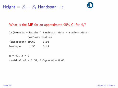
Height = β0 + β1 Handspan +ε
What is the ME for an approximate 95% CI for β1?
lm(formula = height ~ handspan, data = student.data)
coef.est coef.se
(Intercept) 39.60 3.96
handspan 1.36 0.19
---
n = 80, k = 2
residual sd = 3.56, R-Squared = 0.40
Econ 103 Lecture 22 – Slide 18

Simple vs. Multiple Regression
Terminology
Y is the “outcome” and X is the “predictor.”
Simple Regression
One predictor variable: Yi = β0 + β1Xi + εi
Multiple Regression
More than one predictor variable:
Yi = β0 + β1Xi1 + β2Xi2 + . . .+ βkXik + εi
I In both cases ε1, ε2, . . . , εn ∼ iid(0, σ2)
I Multiple regression coefficient estimates β1, β1, . . . , βk
calculated by minimizing sum of squared vertical deviations,
but formula requires linear algebra so we won’t cover it.
Econ 103 Lecture 22 – Slide 19

Interpreting Multiple Regression
Predictive Interpretation
Yi = β0 + β1Xi1 + β2Xi2 + . . .+ βkXik + εi
βj is the difference in Y that we would predict between two
individuals who differed by one unit in predictor Xj but who had
the same values for the other X variables.
What About an Example?
In a few minutes, we’ll work through an extended example of
multiple regression using real data.
Econ 103 Lecture 22 – Slide 20
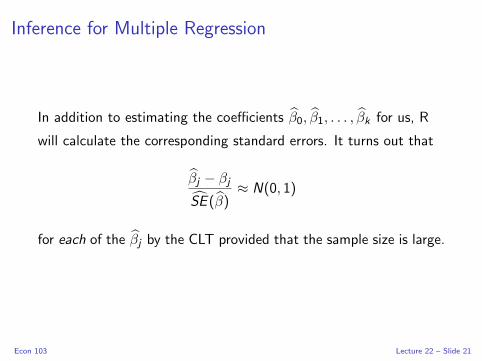
Inference for Multiple Regression
In addition to estimating the coefficients β0, β1, . . . , βk for us, R
will calculate the corresponding standard errors. It turns out that
βj − βj
SE (β)≈ N(0, 1)
for each of the βj by the CLT provided that the sample size is large.
Econ 103 Lecture 22 – Slide 21

Height = β0 + β1 Handspan +ε
What are residual sd and R-squared?
lm(formula = height ~ handspan, data = student.data)
coef.est coef.se
(Intercept) 39.60 3.96
handspan 1.36 0.19
---
n = 80, k = 2
residual sd = 3.56, R-Squared = 0.40
Econ 103 Lecture 22 – Slide 22
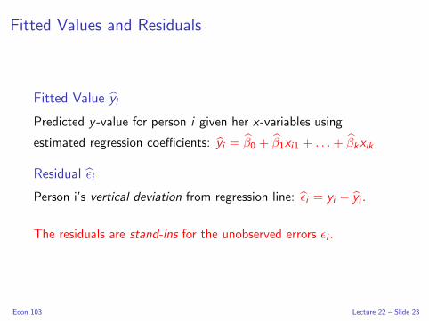
Fitted Values and Residuals
Fitted Value yi
Predicted y -value for person i given her x-variables using
estimated regression coefficients: yi = β0 + β1xi1 + . . .+ βkxik
Residual εi
Person i’s vertical deviation from regression line: εi = yi − yi .
The residuals are stand-ins for the unobserved errors εi .
Econ 103 Lecture 22 – Slide 23

Residual Standard Deviation: σ
I Idea: use residuals εi to estimate σ
σ =
√∑ni=1 ε
2i
n − k
I Measures avg. distance of yi from regression line.
I E.g. if Y is points scored on a test and σ = 16, the regression
predicts to an accuracy of about 16 points.
I Same units as Y (Exam practice: verify this)
I Denominator (n − k) = (# Datapoints - # of X variables)
Econ 103 Lecture 22 – Slide 24
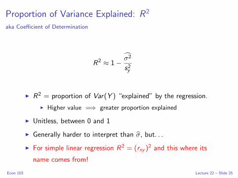
Proportion of Variance Explained: R2
aka Coefficient of Determination
R2 ≈ 1− σ2
s2y
I R2 = proportion of Var(Y ) “explained” by the regression.
I Higher value =⇒ greater proportion explained
I Unitless, between 0 and 1
I Generally harder to interpret than σ, but. . .
I For simple linear regression R2 = (rxy )2 and this where its
name comes from!
Econ 103 Lecture 22 – Slide 25

Height = β0 + β1 Handspan +ε
lm(formula = height ~ handspan, data = student.data)
coef.est coef.se
(Intercept) 39.60 3.96
handspan 1.36 0.19
---
n = 80, k = 2
residual sd = 3.56, R-Squared = 0.40
> cor(student.data$height, student.data$handspan)^2
[1] 0.3954669
Econ 103 Lecture 22 – Slide 26

Which Gives Better Predictions: Sex (a) or Handspan (b)?
lm(formula = height ~ sex, data = student.data)
coef.est coef.se
(Intercept) 64.46 0.56
sexMale 6.10 0.76
---
n = 80, k = 2
residual sd = 3.38, R-Squared = 0.45
lm(formula = height ~ handspan, data = student.data)
coef.est coef.se
(Intercept) 39.60 3.96
handspan 1.36 0.19
---
n = 80, k = 2
residual sd = 3.56, R-Squared = 0.40
Econ 103 Lecture 22 – Slide 27

Bring Your Laptop Next Time:
We’ll be Using R
Econ 103 Lecture 22 – Slide 28


![3.2 6.6 NYCON USED ON 215 4.2 32 2.5 OR (REVISION RECORD; 2 … · 2015-11-18 · 3.2 6.6 nycon used on 215 4.2 32 2.5 or (revision record; 2-poa customer drawing o ysk] (material)_.](https://static.fdocuments.us/doc/165x107/5f65ca506a664b2505403764/32-66-nycon-used-on-215-42-32-25-or-revision-record-2-2015-11-18-32-66.jpg)