DEPARTMENT OF ECONOMICS

Economic Value of Stock and Interest

Rate Predictability in the UK

Stephen Hall, University of Leicester, UK Kevin Lee, University of Leicester, UK

Kavita Sirichand, University of Leicester, UK

Working Paper No. 10/13 April 2010

Updated August 2010

The Economic Value of Stock and Interest Rate

Predictability in the UK�

Stephen Hall, Kevin Leeyand Kavita SirichandUniversity of Leicester, UK

August 2010

Abstract

This paper examines asset return predictability by comparing the out-of-sampleforecasting performance of both atheoretic and theory informed models of bond andstock returns. We evaluate forecasting performance using standard statistical crite-rion, together with a less frequently used decision-based criterion. In particular, foran investor seeking to optimally allocate her portfolio between bonds and stocks, weexamine the impact parameter uncertainty and predictability in returns have on howthe investor optimally allocates. We use a weekly dataset on UK Treasury Bill ratesand the FTSE All-Share Index over the period 1997 to 2007. Our results suggest thatin the context of investment decision making under an economic value criterion, theinvestor gains from not only assuming predictability but by modelling the bond andstock returns together.

Keywords: density forecasting, decision-based forecast evaluation, interest rateand stock return models, predictability and parameter uncertainty.

JEL Classi�cations: C32, C53, E43, E47

�We are grateful to Giorgio Valente for his helpful comments. Corresponding author: Kavita

Sirichand, Department of Economics, University of Leicester, Leicester, LE1 7RH, UK, email:

kayess62@googlemail.com.yStephen Hall and Kevin Lee would like to acknowledge the support of ESRC Grant Number RES-062-

23-1753.

1 Introduction

Evidence of predictability in asset returns has been reported by a number of studies

including Campbell (1987), Fama and French (1988a,b and 1989), Kandel and Stambaugh

(1996) and Ang and Bekaert (2007). They show variables including the dividend yield

and term structure variables, have predictive power for the stock return. This overturning

the long standing view held up until the 1970s in �nancial economics, that returns are

not predictable. Most of this evidence is based on studies that assess predictability from

a statistical standpoint, using measures like the signi�cance of estimated coe¢ cients, the

explanatory power of the regressors and the RMSEs of forecasts.

However, recent research argues that conventional statistical forecast evaluation crite-

ria, usually based on some measure of the forecasts error, may be inappropriate. Instead,

it would be more appropriate to evaluate forecast accuracy using pro�tability, given �rms

use forecasts to increase pro�ts, Leitch and Tanner (1991). Further, Granger and Pesaran

(2000) and Pesaran and Skouras (2004) argue that forecasts should be evaluated in the

decision making context for which they are intended. These studies advocate the use of

decision-based forecast evaluation1, where forecasts are judged in terms of their economic

value to the user, rather than in terms of forecast errors.

This paper �rst examines the impact of predictability in bond and stock returns,

together with the e¤ect of parameter uncertainty upon how an investor optimally allocates

her portfolio. Second, we consider if there is any economic value to the investor of bond

and stock return predictability.

Authors including West, Edison and Cho (1993), Pesaran and Timmermann (1995),

Xia (2001), Brooks and Persand (2003), Avramov (2002), Boudry and Gray (2003), and

Marquering and Verbeek (2004) have previously considered the economic value of pre-

dictability in returns within an asset allocation framework. Barberis (2000) considers

how asset return predictability a¤ects optimal portfolio choice for long horizon investors,

if this allocation di¤ers with the investment horizon and further the impact on allocation

when parameter uncertainty2 is incorporated3. Barberis de�nes no predictability as the

investor assuming that stock returns are i.i.d. and predictability as him believing that a

single lagged dividend yield term has predictive power for stock returns. In both cases

bond returns are assumed constant. Predictability has the e¤ect of making stocks look

less risky and parameter uncertainty makes them look more so. Barberis demonstrates

that the investment horizon may not be irrelevant if returns are predictable. Further,

even with parameter uncertainty there is su¢ cient predictability of returns, such that

investors allocate signi�cantly more to stocks the longer the horizon and that those who

ignore parameter uncertainty over allocate to stocks by a considerable amount.

1We may also refer to economic value measures, these are the same as decision-based measures.2Earlier studies by Klein and Bawa (1976), and Kandel and Stambaugh (1996) demonstrate the impor-

tance of parameter uncertainty in asset allocation.3He uses monthly US data for two assets: T-bills and the stock index to examine the potential horizon

e¤ects under buy-and-hold and dynamic optimal rebalancing strategies, in discrete time for an investor

with power utility over terminal wealth.

1

Recent studies that examine the predictive power of theory informed models under

decision-based criteria for exchange rates include Abhyankar, Sarno and Valente (2005,

henceforth ASV) and Garratt and Lee (2009, GL). Both �nd evidence of economic value

to exchange rate predictability, in that the realised terminal wealth of an investor who

assumes predictability is higher than that of the investor who assumes no predictability.

For interest rates, Della Corte, Sarno and Thornton (2008, DST) assess the validity of

the Expectations Hypothesis (EH) of the term structure of interest rates, to �nd that on

the basis of statistical tests the EH is rejected, but from an economic value perspective

favourable support is found.

The results reported by ASV, DST and GL illustrate that the forecasting performance

of models can be signi�cantly di¤erent depending on whether statistical or decision-based

evaluation techniques are used. To re-iterate the point made in Hall et al (2010), under

statistical measures atheoretic models like the random walk are di¢ cult to beat. But

under economic value methods encouraging evidence in favour of predictability, as captured

by theory informed models, is found. The studies described here bring to our attention

several key factors including the importance of predictability and parameter uncertainty

in asset allocation, generating density forecasts to capture the risk as well as the return

of the asset and the economic value to the investor of these forecasts.

The contributions of this paper are empirical. To my knowledge we are the �rst to

model both bond and stock returns, separately and jointly, and evaluate their predictability

in an asset allocation setting using economic value. Chordia et al (2005, pp. 87) argue

that "A negative information shock in stocks often causes a "�ight to quality" as investors

substitute safe assets for risky assets". Further, "when stocks are expected to show

weakness, investment funds often �ow to the perceived haven of the bond market, with that

shift usually going into reverse when, .., equities start to strengthen." Party (2001, cited in

Chorida et al (2005))4. Both of these statements highlight the dynamic relationship that

exists between bond and stock markets, this supports the need to model them together

and try to capture these interactions. That is, allow for the possibility that the variables

of one market have explanatory power for the variables of the other.

In brief, we compute the optimal portfolio allocation for a buy-and-hold investor with

power utility over terminal wealth using weekly UK data during 1997 week 10 to 2007 week

19 for two assets, the 1-month T-bill and the FTSE All-Share Index. We extend the work

of Barberis by allowing for the possibility of predictability in bond returns too and further

model the bond and stock returns jointly. Here under predictability the investor assumes

past values of the asset returns together with key stock and term structure variables, like

the dividend yield and interest rate spreads have explanatory power. We consider a set of

four models that assume varying degrees of bond and stock return predictability, all under

a VAR framework. We examine the impact predictability and parameter uncertainty have

on how the investor optimally allocates her portfolio. Both statistical and decision-based

criteria are used to evaluate the out-of-sample forecasting performance of the models, to

4Full reference is John Party, The Wall Street Journal, 1st August 2001, pp. C1.

2

ascertain if indeed there is economic value to bond and stock return predictability.

Our results do suggest that in the context of investment decision making under an

economic value criterion, the investor allocates di¤erently when she assumes predictability

to an investor who assumes that returns are not predictable. Moreover, she gains from

not only assuming predictability in both returns, but by modelling the bond and stock

returns jointly.

The setup of this paper is as follows Section 2 details how we model the interest rates

and stocks, the investment decision and the framework used to evaluate the economic value

of predictability when parameter uncertainty is both ignored and accounted for. Section

3 describes the dataset, the estimated models and provides a statistical evaluation of the

forecasting performance of each model. In Section 4 we judge the models� forecasting

performance by comparing the realised end-of-period wealth generated under each and

Section 5 concludes.

2 Optimal Allocation, Parameter Uncertainty & Predictabil-ity

We examine how a utility-maximising investor allocates her portfolio between 1-month

T-bills and the FTSE All-Share Index. That is, between the stock market and risk-free

bonds. We consider if there are gains in utility for an investor, who employs a theory

informed model to forecast interest rates and stock returns, in comparison to one who

believes that the returns are not predictable. Here we describe the models estimated

when we �rst ignore T-bill and stock return predictability and then when we consider

predictability. Further, we introduce how we measure the economic value of interest rates

and stock returns under predictability and parameter uncertainty.

When considering the predictability in interest rates we look to the EH of the term

structure of interest rates. It suggests that a n-period long rate is given by a weighted

average of current and future expected short m-period rates over n periods with the ad-

dition of a time invariant term premium. A further formulation of the EH describes the

yield spread by expected changes in the future short rate. If the yields share a common

stochastic trend then (q � 1) cointegrating vectors should exist, as implied by stationarybivariate spreads, in a set of q non-stationary yields. Assuming that yields are di¤erence

stationary and that there exists a cointegrating relationship between the n- and m-period

yields, then there exists a Wold representation which can be approximated by a VAR(p)

model that describes the change in the m-period rate and the spread between the n- and

m-period yields using past changes and spreads, see Campbell and Shiller (1991)5. Here

we use this VAR model, that embeds the cointegration implied by the EH to explain the

term structure and in turn forecast the yields. As such, we proceed assuming that if the

5Numerous tests of the EH have been carried out using various datasets and testing methods, with the

evidence in support of the EH being somewhat mixed, see Campbell and Shiller (1991); Taylor (1992);

Cuthbertson (1996); Cuthbertson, Hayes & Nitzsche (1996, 2003); Longsta¤ (2000); Sarno, Thornton and

Valente (2007).

3

investor believes bill returns are predictable she uses past yield changes and spreads to

forecast future returns. For the stock returns we follow previous studies including Kandel

and Stambaugh (1996) and Barberis (2000), and use the dividend yield to examine stock

return predictability. Such that if the investor believes stock returns are predictable she

uses dividend yields to forecast future returns.

2.1 Modelling Interest Rates and Stocks

Let rst be the return on the FTSE All-Share Index in week t, r(1)t be the return on a

1-month T-bill, both returns are continuously compounded monthly returns. dyt is the

dividend yield, the change in the 1-month T-bill rate �r(1)t = r(1)t � r(1)t�1 and the spread

between a n- and 1-month rate s(n;1)t = r(n)t � r(1)t for n = 3; 6; 12. We refer to rst and dyt

as the stock variables, and �r(1)t and s(n;1)t as the bond (or term structure, TS) variables.

In order to determine how the investor should optimally allocate her portfolio she requires

forecasts of r(1)t and rst : We consider four alternative models from which the investor could

derive these forecasts, generally each model can be summarised by the following VAR(p)

xt = �+

pXi=1

Bixt�i + �t (1)

where xt is a (q � 1) vector of variables, Bi is a (q � q) matrix of parameters, � is a(q � 1) vector of intercepts and �t is assumed to be a (q � 1) vector containing i:i:d seriallyuncorrelated errors with zero means and a positive de�nite covariance matrix �. The

exact composition of xt will depend upon the assumption made regarding predictability,

as detailed below.

The VAR framework enables one to examine how predictability a¤ects portfolio allo-

cation by changing the variables in the VAR. We propose four models for predicting the

returns on the T-bill and stock index, each incorporating varying degrees of predictability:

Barberis Non Predictability (BNP), Barberis Predictability (BP), Individual VARs (IV)

and the Joint VAR (JV) model.

The Barberis Non Predictability and Predictability models are named so, since they

are in the spirit of those estimated by Barberis (2000). These models assume that the

risk-free T-bill rate r(1) is constant6 and allow only for the possibility of predictability in

stock returns. Under the assumption of no predictability as in the BNP model, there are

no predictor variables in the VAR, the stock index returns are assumed to be i:i:d: such

that rst = �+ �t, i.e. a drift term plus a random error term. Hence xt = rst and Bi = 0:

However, under the assumption of predictability as in the BP model, the dividend yield

is included in the VAR, with xt = (rst ; z0t)0, zt = (z1;t; :::; zn;t)

0 and xt = � + Bzt�1 + �t.

Such that zt is a vector containing explanatory variables for the stock index return, i.e.

the dividend yield. Hence the �rst equation of the VAR speci�es the expected stock index

return as a function of the dividend yield, and the second equation speci�es the stochastic

evolution of the dividend yield.6The T-bill rate is assumed constant at the last value of the estimation sample, such that in the �rst

recursion it is �xed at its 2004 week 18 value.

4

Further, it is possible to relax this assumption of a constant T-bill rate and allow for

predictability in both T-bill and stock returns, we do this in two ways. First, using the IV

model, where the predictability of T-bill and stock returns are described separately by two

VARs (IV-BOND and IV-STOCK). The form of xt for the bond returns and the stock

returns are given by x(1)t =��r

(1)t ; s

(12;1)t ; s

(6;1)t ; s

(3;1)t

�0and xst = (rst ; dyt)

0 respectively.

Second, using the JV model, where the predictability of the bill and stock returns are

modelled jointly within a single system, here xt =�rst ; dyt;�r

(1)t ; s

(12;1)t ; s

(6;1)t ; s

(3;1)t

�0:

By modelling the predictability of T-bill and stock returns in these two ways allows

us to test whether it is bene�cial to the investor, in terms of wealth gains, to model the

two returns jointly. In that, by allowing for interactions and feedbacks to exist between

the bond and stock market, will the investor who uses the JV model to generate forecasts

of the T-bill rate and the return on stocks achieve a higher wealth? Each of these four

models are estimated when the parameter uncertainty, which is the uncertainty about the

true values of the model�s parameters, is both ignored and accounted for7.

In time T the buy-and-hold investor faces the problem of how to optimally allocate

her wealth over a H month investment horizon between 1-month T-bills and the FTSE

All-Share Index, where these two assets yield the continuously compounded returns r(1)Tand rsT respectively.

With an initial wealth of WT = 1 and ! being de�ned as the proportion of initial

wealth allocated to bonds8, the end-of-horizon wealth is given by

WT+H = ! exp

�HPi=1r(1)T+i�1

�+ (1� !) exp

�HPi=1rsT+(i�1)

�(2)

Further, risk aversion can be incorporated into the investor�s decision making, by

assuming that the utility gained from the end-of-horizon wealth follows that given by a

constant relative risk-aversion (CRRA) power utility function.

�(W ) =W 1�A

1�A (3)

where A is the coe¢ cient of risk aversion. The optimisation problem faced by the investor

in T is

max!ET f�(WT+H (!)) j T g (4)

where the investor computes the expectation above conditional upon the information set

available at T . Fundamental to this optimisation problem is the distribution the investor

employs to evaluate this expectation. The distribution used depends upon whether the

investor assumes predictability in bond and stock returns. To ascertain the in�uence of

predictability on allocation decisions, a comparison between the allocations of an investor

7We di¤erentiate between when the model is estimated subject to stochastic uncertainty only, and when

it is estimated subject to stochastic and parameter uncertainty by denoting them as BNP, BP, IV, JV and

BNPPU, BPPU, IVPU, JVPU respectively.

8Under the BNP and BP models the T-bill return is assumed to be constant, such thatHPi=1

r(1)

T+(i�1) =

H:r(1).

5

who ignores predictability, to that of one who takes it into account can be made. This

will now be discussed in greater detail below.

2.2 The Predictive Density Function

In this section we discuss the approach taken to estimate the density function in the case

where parameter uncertainty is not considered and when it is. The form of the density

P (XT+1;H j XT ) is determined by the types of uncertainty surrounding the forecasts, andhow the function is characterised and estimated. Here we follow the method proposed by

Garratt, Lee, Pesaran and Shin (2003 and 2006, GLPS) and GL, which takes a classical

view of the Bayesian approach9 to calculating the density function. This involves approx-

imations of certain probabilities of interest, thereby avoiding the need for priors. We will

now provide a summary of the methods described in GLPS and GL.

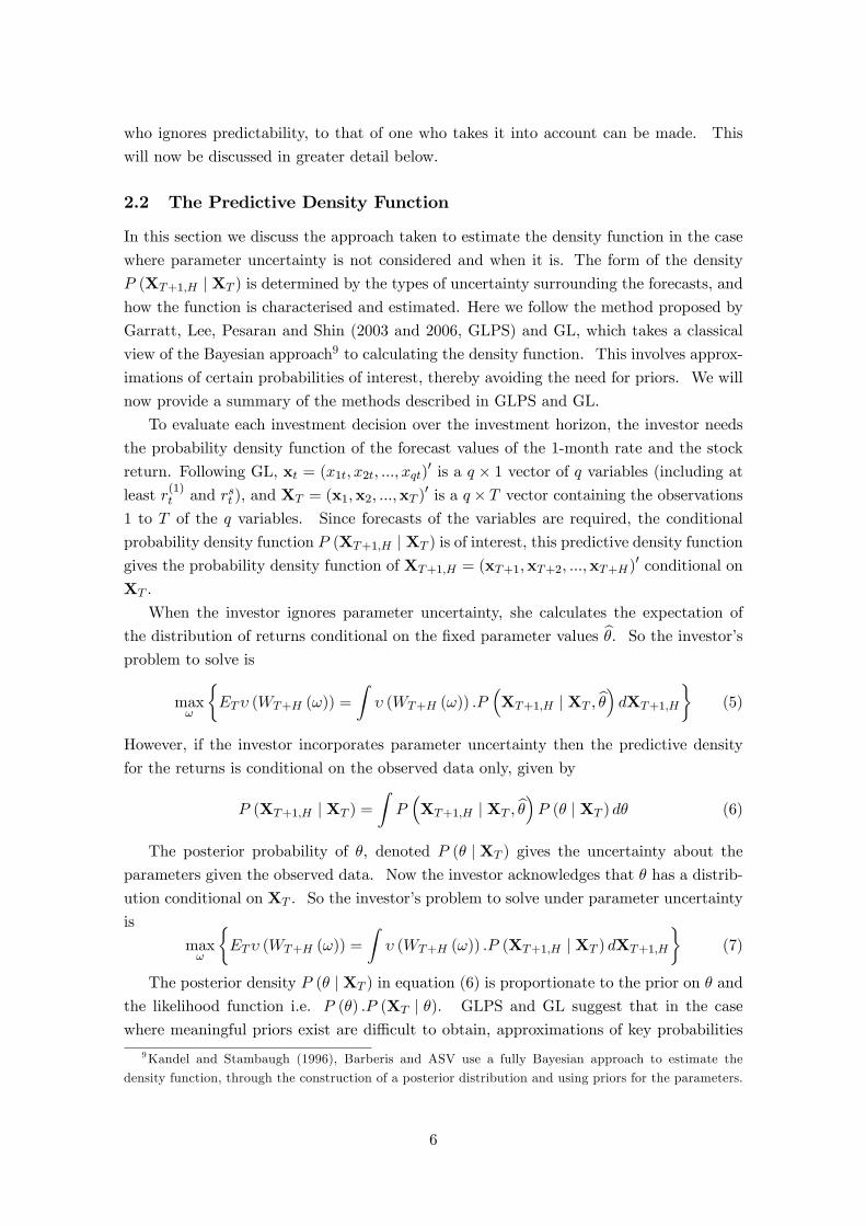
To evaluate each investment decision over the investment horizon, the investor needs

the probability density function of the forecast values of the 1-month rate and the stock

return. Following GL, xt = (x1t; x2t; :::; xqt)0 is a q � 1 vector of q variables (including at

least r(1)t and rst ), and XT = (x1;x2; :::;xT )0 is a q � T vector containing the observations

1 to T of the q variables. Since forecasts of the variables are required, the conditional

probability density function P (XT+1;H j XT ) is of interest, this predictive density functiongives the probability density function of XT+1;H = (xT+1;xT+2; :::;xT+H)

0 conditional on

XT :

When the investor ignores parameter uncertainty, she calculates the expectation of

the distribution of returns conditional on the �xed parameter values b�. So the investor�sproblem to solve is

max!

�ET� (WT+H (!)) =

Z� (WT+H (!)) :P

�XT+1;H j XT ; b�� dXT+1;H� (5)

However, if the investor incorporates parameter uncertainty then the predictive density

for the returns is conditional on the observed data only, given by

P (XT+1;H j XT ) =ZP�XT+1;H j XT ; b��P (� j XT ) d� (6)

The posterior probability of �, denoted P (� j XT ) gives the uncertainty about theparameters given the observed data. Now the investor acknowledges that � has a distrib-

ution conditional on XT . So the investor�s problem to solve under parameter uncertainty

is

max!

�ET� (WT+H (!)) =

Z� (WT+H (!)) :P (XT+1;H j XT ) dXT+1;H

�(7)

The posterior density P (� j XT ) in equation (6) is proportionate to the prior on � andthe likelihood function i.e. P (�) :P (XT j �). GLPS and GL suggest that in the case

where meaningful priors exist are di¢ cult to obtain, approximations of key probabilities

9Kandel and Stambaugh (1996), Barberis and ASV use a fully Bayesian approach to estimate the

density function, through the construction of a posterior distribution and using priors for the parameters.

6

needed to estimate the predictive density P (XT+1;H j XT ) can be used. They assume forthe posterior probability of �

� j XT!~N

�b�T ; T�1 bV�� (8)

where b�T is the maximum likelihood estimate of the true parameter value of �, and T�1 bV�is the asymtotic covariance matrix of b�T i.e. of the estimated parameters.

In this exercise we consider stochastic and parameter uncertainty, the uncertainty as-

sociated with the model and the estimated model parameters respectively. We appreciate

that interest rates and stock returns can be modelled under various assumptions, and thus

model the two returns in four di¤erent ways: BNP, BP, IV and JV models as described

above, which can all be summarised by equation (1).

For each of these models, through stochastic simulation techniques, an estimate of the

probability density function of the forecasts can be computed. Given that these simula-

tions provide an estimate of the predictive densities P�XT+1;H j XT ; b�� when parameter

uncertainty is ignored and P (XT+1;H j XT ) when it is considered, it is now possible toevaluate ET (� (WT+H) j T ) for a range of portfolio weights !: That is, � (WT+H (!)) is

computed eR times for each value of !: Then the mean across these eR replications is cal-culated, from which the investor chooses the weight ! that maximises the expected utility

ET� (WT+H (!)) : Here ! takes values 0, 0.01,...,0.99,1, where ! = 0 suggests all should

be allocated to bills, equally ! = 1 suggests that all should be allocated to stocks. The

weight is between 0 and 1, so we do not allow for short selling. Details of the estimation

procedure, how the computations are carried out and the method by which the errors are

calculated 10 are provided in Appendix A.

3 Modelling the UK Treasury Bill Rates and the FTSE All-Share Index

3.1 Returns Data

In this study we use weekly observations on the continuously compounded monthly returns

for both the 1-month T-bill11 r(1)t and the FTSE All-Share Index12 rst , and the dividend

yield dyt for the UK. These variables together with �r(1)t ; s

(3;1)t ; s

(6;1)t and s(12;1)t are used

in the analysis, refer to the Data Appendix for the de�nitions, sources and transformations

conducted. The entire sample period is from 1997 week 10 to 2007 week 19 (532 observa-

tions). Figures 1 and 2 plot the monthly stock return, the dividend yield, the monthly bill

return in levels and �rst di¤erences, and the three spreads over the entire sample. The10The errors can be drawn using either parametric or non-parametric methods (see GLPS (2006) p166-

168), here parameteric methods are utilised where the errors are assumed to be i:i:dN (0;�) serially

uncorrelated white noise errors.11The estimated yield curve data is used as opposed to actual T-bill data here, because data was

unavailable during some periods of our sample. However, we are satis�ed that the data used here is a fair

re�ection of what the investor would get, should she want to undertake an investment in T-bills.12We use the FTSE All-Share Index since it gives a broad portfolio of stocks.

7

monthly stock return takes an average value of 0.59% compared with 0.41% for the T-bill,

with a minimum and maximum of -17.72 to 15.32% and 0.26 to 0.60% respectively over

the whole sample. This corresponds to what we would expect, average returns from the

stock market tend to be higher, but there is a risk of making a loss. The return from the

1-month T-bill has a general downward trend up until the end of 2004, before increasing

until the end of the sample. The annual dividend yield takes an average value of 2.86%,

although there are some persistent deviations, the dividend yield exhibits mean reversion.

The yield di¤erence and spreads display mean reverting behaviour which is consistent with

a stationary process.

The four models are each estimated over the period 1997 week 10 to 2004 week 18

(374 observations) and then recursively at weekly intervals through to 1997 week 10

to 2005 week 18 (427 observations), giving 54 recursions in total. For each recursion

we generate h-step ahead out-of-sample forecasts13 for h = 1; 2; :::;H; ::: and the in-

vestment horizon H = 3; 6; 12; 18 and 24 months. So for the �rst recursion we fore-

cast over the period 2004 week 19 to 2006 week 18 and for the last recursion 2005

week 19 to 2007 week 19. For each recursion the investor will use his generated fore-

casts to determine the optimal allocation of his portfolio. Hence in this exercise we

will have 54 allocation decisions for each A and H, with which to compare the al-

locations and utility gains under each model without and with parameter uncertainty.

3.2 Estimating the Models

Here we describe how we estimate the four models and present the estimated regression

results for the �rst recursion14 over 1997 week 10 to 2004 week 18. We begin by employing

the ADF, PP and KPSS unit root tests to determine the order of integration of rst , dyt,

r(1)t , s

(3;1)t ; s

(6;1)t and s(12;1)t over the entire sample period, see Table 1. All three tests

indicate that rst and the spreads are found to be stationary in levels and r(1)t is di¤erence

stationary. As for dyt the unit root tests suggest it is non-stationary, but given the test

statistics are close to their respective critical values and the series exhibits mean reversion

we treat, like in previous studies, the dividend yield as stationary.

The optimal lag length for the IV and JV models is chosen by estimating a set of

VAR(p) with p = 0; 1; :::; 12 for each model over 1997 week 10 to 2004 week 18. The

optimal lag length is that which minimises the Schwarz Information lag selection criteria,

as well as satisfying the diagnostic checks, in particular the model�s residuals should be

free of serial correlation at the 5% level. Based on this, the lag length chosen was �ve for

the IV-STOCK model, six for the IV-BOND and JV models. Tables 2 to 8 summarise

the estimates with the diagnostics of the BNP, BP, IV and JV models.

13We denote the investment horizon H in months since r(1)t and rst are monthly returns. However, the

data has a weekly frequency, so when we refer to the �h-step�ahead forecasts each �step�is a week.14Estimates of each model for the �rst recursion only are provided, to give an overall impression of the

in-sample predictability. At the forecasting stage the models are estimated recursively.

8

Comparing the estimated BP model to the BNP model, Table 2 to 3, there is a small

gain in explanatory power by allowing for predictability in stock returns through the

inclusion of a single lagged dividend yield term. Further, all coe¢ cients in the estimated

BP model are signi�cantly di¤erent from zero. Moving from the BP to the IV-STOCK

model, Table 3 to 4, allows for past values of both rs and dy to in�uence current values.

A substantial gain in explanatory power for stock returns is observed. All the coe¢ cients

are jointly signi�cant, which suggests there are gains from relaxing the assumptions of no

and limited predictability made under the BNP and BP models. For each equation in

the IV-BOND model, Tables 5 and 6, the TS15 variables are jointly signi�cant. The JV

model, Table 7 and 8, is a generalisation of the individual VARs, allowing for feedbacks

between the two markets. In terms of explanatory power as indicated by R2, the gains

from modelling the two returns together are small. However, the stock variables are jointly

signi�cant in all the TS equations, but the TS variables are jointly signi�cant in the TS

equations only. This implies that causality exists from the stock market variables to the

TS variables, which provides support in favour of modelling the two markets together.

The diagnostics are satisfactory, there is indication of some serial correlation in the

stock equations of the BNP and BP models, but we want to replicate those estimated in

Barberis. In the IV and JV models we do not have serial correlation at the 5% level

and the explanatory power of the models is quite high. Rejection of the nulls that the

regression residuals are homoskedastic and normal is not surprising given that we are using

�nancial data. But we follow the assumptions made by the literature that also utilise

such data.

3.3 Statistical Forecast Evaluation

The root mean squared error (RMSE) provides a statistical evaluation of the out-of-sample

forecasting performance of each model. Table 9 gives the RMSEs of the bond and stock

return forecasts, for the forecast horizons H = 1; 3; 6; 12; 18 and 24 months for each model,

without and with parameter uncertainty being considered. Table 10 reports the ratio of

the RMSEs for each model to the benchmark model. A value of the ratio greater than

one indicates that the RMSE of the model is lower than that of the benchmark. The

benchmark taken is the BNP model which assumes r(1)t is constant and rst = �+�t, since it

assumes no predictability a comparison can be made with the other models which assume

varying degrees of predictability.

The RMSEs for forecasts of the bond returns indicate that only at H = 1 do the JV

and JVPU models beat the benchmark. The BNP, BP, BNPPU and BPPU models that

make the strong assumption that r(1)T+H is constant, outperform the other more theory

informed models at each horizon under this criteria. However, it can be seen that the

di¤erences in the RMSEs amongst the models are small. These results broadly correspond

to those found in the exchange rate forecasting literature, as summarised in ASV and GL.

Which in general �nd sophisticated theory informed models are outperformed by a simple

15TS is used to denote the term structure. The TS variables are �r(1)t ; s(3;1)t ; s

(6;1)t and s(12;1)t .

9

random walk.

With the stock returns, the RMSEs show that there is not a single model that performs

consistently well over all horizons. The JV and JVPU models perform the best atH = 1; 3

and 12, whereas the BP and BPPUmodels perform well atH = 6; 18 and 24. These results

suggest some gain in terms of forecasting performance from incorporating predictability

when modelling stock returns.

When comparing the size of the RMSEs of the two returns, there is greater variance

in the rst forecasts than the r(1)t forecasts. This is not surprising since stock returns are

more volatile and thus more di¢ cult to predict. In general, the RMSEs increase up until

H = 6 and 12 before decreasing. This suggests that the RMSEs for both the returns

are non-monotonic, i.e. they oscillate in relative value and do not just increase with H.

Although the RMSEs for both the returns are non-monotonic, the rates at which the two

are changing across the horizons are di¤erent. Over the shorter horizon, the rate at which

the RMSEs for r(1)t increase is smaller than the rate at which the RMSE for rst increases.

But over the longer horizon the rate at which the RMSE for r(1)t decreases is greater.

This statistical evaluation provides an indication of the forecasting performance of

each model. But does not provide a clear indication of how these models perform in an

investment decision making context, i.e. in terms of the economic value of the gains from

the models�forecasts.

4 E¤ects on Allocation

We now examine the implications for optimal allocations when the returns are either i.i.d.

or predictable, where the degree of predictability is varied and parameter uncertainty

is both ignored and accounted for. In the case where parameters are assumed �xed

the maximisation problem is given by equation (5) and under parameter uncertainty it

is given by (7). Figures 3 to 7 give the optimal allocations to bonds, 100!%, at each

investment horizon H = 3; 6; 12; 18; 24 months, for each model and for the levels of risk

aversion A = 2; 5 and 10; A = 10 is the highest level of risk aversion: The models are

estimated �rst over 1997 week 10 to 2004 week 18, the optimal weights are calculated

from the forecasts generated from each estimated model. Then moving forward one week

this is repeated, re-calculating expected wealth and utility to �nd the optimal weight for

this new augmented sample. This is repeated for each recursion, giving results for 54

recursions over the total evaluation period 2004 week 19 to 2007 week 19. The plots are

based on the optimal allocation averaged over the 54 recursions for a particular A, H and

model.

Figure 3 gives the optimal allocation under each model, when parameter uncertainty is

ignored, here allocations are conditional on the �xed parameter values estimated. A risk

aversion e¤ect is evident for all the models, where the investor allocates more to bonds

at all horizons the more risk averse she is. Further, under the BP, IV and JV models

the di¤erence in the allocation to bonds under each A increases with H, with di¤erences

of up to 65% being observed for an investor with A = 2 compared with A = 10. This

10

suggests that the allocation to bonds for a longer horizon investor greatly depends on how

risk averse they are.

It can be seen that the investment horizon is also important in determining how the

investor allocates. In the absence of horizon e¤ects, the short horizon investor allocates no

di¤erently than a long horizon investor. With horizon e¤ects there is a di¤erence betweenthe allocations of a short and long horizon investor, such that the �allocation curve�which

we de�ne as describing for a particular A how the investor allocates over H, has a slope.

Further, this curve may have a positive or negative slope, if the slope is positive then the

investor allocates more to bonds as H increases. Here strong horizon e¤ects are present

under all models. In general, we �nd as H increases under the BNP and BP models the

investor allocates more to bonds for all A. This is true for A = 5 and 10 under the IV

model, but for A = 2 the allocation to stocks increases with H. Equally, under the JV

model for A = 10 the investor increases her allocation to bonds with H, for A = 5 she

increases the allocation to stocks over the medium horizon before increasing the allocation

to bonds in the longer horizon, whereas with A = 2 the investor increase her allocation to

stocks with H.

In short, horizon e¤ects are present. But the extent of the e¤ect the investment

horizon has on the allocation depends upon the predictability assumptions the investor

makes. That is, which model she believes to be true and her level of risk aversion.

We will now try and provide an explanation for these allocation results by �rst con-

sidering the e¤ects of predictability (ignoring parameter uncertainty) and then the e¤ects

of parameter uncertainty.

4.1 Predictability E¤ects

In this exercise we consider four di¤erent models for forecasting interest rates and stock

returns. The atheoretic BNP and BP models assume no predictability in regard to bond

returns. Further, the BNP model assumes no variables are able to predict the stock

return. However, the BP model relaxes this assumption allowing for some predictability

in stock returns. On the opposite end of the spectrum, the theory informed IV and JV

models not only assume predictability, but as in the case of the JV model allow for the

possibility of feedbacks amongst the stock and term structure variables.

These models re�ect opposing views of whether bond and stock returns are predictable,

and further have a varying degree of predictability which increases as we move from the

BNP to BP to IV to JV model. If the investor assumes no predictability then she believes

in the BNP model. Conversely, if she assumes predictability she may believe in the BP,

IV or JV model depending on the extent of the predictability assumed. Ultimately, how

the investor allocates is determined by which model she believes to be a true depiction of

reality.

From Figure 3 it can be seen that the BNP model allocates the most to bonds, followed

by the BP, the IV and then the JV model at each A and H. Where the JV model allocates

the most to stocks. The di¤erence in allocation to bonds in some cases is over 70% amongst

11

the models, e.g. H = 24 and A = 2 the BNP model allocates 77% more to bonds than

the JV model.

Under no predictability, which is similar to assuming the stock returns follow a random

walk process, the variance of the cumulative log returns distribution �2 ! 1, i.e. thevariance continues to grow with the horizon. Whereas, when the return is modelled as

a stationary process, as is the case under predictability, then �2 ! long run mean i.e.

mean reversion of the variance of returns. In which case, stocks appear less risky in the

long run and are more attractive to long horizon investors, Fama and French (1988).

Under the BNP model we �nd horizon e¤ects, where the investor allocates more to

bonds as H increases. Under the assumption that log returns are independently and

identically normally distributed (assumption of normality is not necessary for this to hold)

the mean and variance of the cumulative log returns distribution grows proportionally

with the investment horizon16 i.e. H� and H�2 . For the risk averse investor with power

utility function, although return per unit of variance is the same as H increases, the higher

return is coupled with higher risk in absolute terms and since the investor is risk averse

she allocates less to stocks as H increases.

With predictability the investor recognises that rather than the returns being i.i.d.

they may be predictable, as is the case under the BP, IV and JV models. Now returns are

no longer independent, but the distribution of future returns is conditional on the current

and past values of the explanatory variables. In which case the mean and the variance

of the returns no longer grow linearly. Barberis highlights that under predictability the

variance of cumulative log stock returns may grow slower than linearly with H, such that

stocks appear comparatively less risky at longer horizons, resulting in higher allocations

to stocks as H increase.

With the BP model however, we �nd that it is the allocation to bonds that increases

with H. A possible explanation for this is that although we are now incorporating

predictability the gain in terms of explanatory power for stocks returns are small, R2

increases from 0% under the BNP model to just over 2% under the BP model, so the

increase in predictability is not su¢ cient for the investor to increase her allocation to

stocks with the horizon.

The bond returns are also modelled17 under the IV and JV models. So now both

returns will be subject to future uncertainty and ultimately the optimal allocation hinges

on how risky bonds look relative to stocks. With the IV model the investor allocates more

to stocks at all horizons than the BNP and BP models, i.e. allocation curve shifts down

for all A. This can be attributed to two factors, �rstly bond returns now look relatively

16rt;t+H = rt+1+rt+2+ :::+rt+H =) E(rt;t+H) = E (rt+1)+E (rt+2)+ :::+E (rt+H) = H�, where each

return has the same mean (identically distributed) and returns are independent in that one return does

not contain information about the other returns. Further, var (rt;t+H) = var (rt+1) + var (rt+2) + ::: +

var (rt+H) = H�2, where the returns are uncorrelated so there is no covariance term and all the variances

are equal (identically distributed).17Note when bond returns are modelled too, the variance of cumulative log bond returns may also grow

less than linearly with H. So now bond and stock returns may both be subject to these predictability

e¤ects.

12

more risky than they did under the BNP and BP models since the return is no longer

known with certainty. Secondly, stock predictability under the IV model has increased

dramatically, from 2% under the BP model to nearly 70%. Both of these factors make

stocks look more attractive.

Predictability increases further under the JV model, we expect an increase in the

allocation to the asset that has gained most from the increase in predictability. An

increase in the allocation to stocks at each H in comparison to the IV model is observed.

Thus stock returns appear to have gained more from modelling the returns jointly, so that

they appear less risky and the investor is more willing to hold them. For A = 2 stock

return predictability dominates as the investor increases the amount allocated to stocks

as H increases. For A = 5 stock return predictability dominates until H = 12, then

bond return predictability dominates such that the investor allocates more to bonds. For

A = 10 bond return predictability dominates as the investor increases allocation to bonds

with H.

Under the varying degrees of predictability that each model assumes, how the increased

predictability alters the optimal allocation depends, �rstly on which return (bond or stock)

bene�ts more from the predictability e¤ect18. Secondly, how risk averse the investor is.

As we move from the BNP to JV model the investor allocates more to stocks at each H,

so the allocation curves shifts down. This could be because the investor is able to predict

stocks better as we move from the BNP to the JV model, so she is prepared to allocate

more to stocks at every horizon for each A. But most evidently for A = 2, when moving

from BNP through to JV the slope of the allocation curve changes. For the IV and JV

models the investor is prepared to allocate substantially more to stocks at longer horizons,

which could be attributed to �2 growing less than linearly combined with the investor not

being very risk averse. Whereas for A = 10 the investor is very risk averse and increases

her allocation to bonds with H.

4.2 Parameter Uncertainty E¤ects

Figures 4 to 7 compare the allocations under each model when parameter uncertainty is

ignored to that when it is considered. Incorporating parameter uncertainty has the e¤ect

of increasing the variance of the distribution of cumulative returns. Further, the variance

increases faster than linearly with H in the case of i:i:d: returns, when this additional

uncertainty is accounted for. This increase in the variance serves to make the asset seem

riskier at longer horizons.

When the investor believes in the BNP model we indeed �nd that the allocation to

stocks is reduced by 0 to 2% with parameter uncertainty, the e¤ects are small over the

horizons considered. For the BP model this additional uncertainty increases the allocation

to bonds by up to 7%, with the e¤ect of parameter uncertainty decreasing as the investor

becomes more risk averse.18The predictability e¤ect results in the variance of cumulative log returns to grow less than linearly,

making the asset appear less risky at longer horizons.

13

Under the IV and JV models the bond returns are also being modelled, such that they

too are subject to parameter uncertainty. Now bonds look riskier than they did under

the BNP and BP models, so the optimal allocation hinges on which asset is a¤ected by

parameter uncertainty more and hence the riskiness of bonds relative to stocks.

Parameter uncertainty under the IV model has the e¤ect of increasing the allocation

to stocks by 3 to 10% in the short to medium horizon for A = 2 and 5, the increase is

smaller for A = 10, before the allocation to bonds increases in the longer horizon to levels

similar to those when parameter uncertainty is ignored. Here we �nd that the impact of

this uncertainty is di¤erent for each A, where the more risk averse the investor is, the less

willing she is to hold more stocks. Allocations emerge as being non-monotonic over H,

because the investor does not simply increase her allocation to stocks with the horizon,

but the slope of the curve actually changes over H. Over the short to medium horizon

it appears that the e¤ect of parameter uncertainty is greater on bond returns than stock

returns. That is, the variance of the cumulative stock returns is less than that of bonds,

�2rs < �2r1, making stocks look less risky and more being allocated to them. But over

the longer horizon the converse seems true, such that stocks look riskier and the optimal

allocation is equal to that when parameter uncertainty is ignored.

The e¤ect of parameter uncertainty is most apparent under the JV model, with allo-

cations to stocks increasing by up to 4% for A = 2, and by the same margin for A = 5

over the short to medium horizon before the allocation to bonds increases over the longer

horizon by 9 to 13%. The changes in allocation to bonds for A = 10 over the investment

horizon are similar to those observed for A = 5, but of a smaller magnitude. Again

allocations are non-monotonic for A = 5 and 10, in that after H = 12 the parameter

uncertainty risk is less for bonds, thus making them appear more attractive.

To explain the non-monotonic allocations that arise under parameter uncertainty, we

consider how the variances about the distribution of future predicted returns evolve over

the forecast horizon. In this case it is reasonable to expect the RMSEs and the variances

to be closely related, such thatwe use the RMSEs as an indication of how the variances

of the forecasts evolve19. Recall Tables 9 and 10, the non-monotonic RMSEs imply that

the variances of the forecasts are also non-monotonic20. This suggests that the variance

about the forecasts contracts and expands with H, so under parameter uncertainty the

asset will appear more risky at some horizons than at others. Further, the variances of the

two returns oscillate at di¤erent rates, such that the e¤ects of parameter uncertainty will

be di¤erent at di¤erent H, so at some horizons stocks will appear more risky than bonds

and at others less. This non-monotonicity combined with the fact that the variances of

the two returns expand and contract at di¤erent rates could provide an explanation for

the impact of parameter uncertainty observed here.

19Since the �2 gives the dispersion about the mean of the distribution and the RMSE measures the

dispersion about the actual value of a variable. Then the mean of the distribution will equal the actual

value if the distribution is unbiased, thus the RMSE will equal the �2 of the forecast.20Which as Hall and Hendry (1988, pp. 256-7) argue may not be so surprising, since non-monotonic

model standard errors may result in non-monotonic total standard errors.

14

We can see that as the investor becomes more risk averse, she is less prepared to allocate

more to stocks when parameter uncertainty is incorporated. Further, she is prepared to

allocate more to stocks under parameter uncertainty over the short to medium horizon,

but not at the longer horizons. Boudry and Gray (2003, BG) also �nd "negative horizon

e¤ects", where the investor allocates more to bonds at longer horizons. This is contrary

to Barberis, who �nds that parameter uncertainty reduces not eliminates the positive

horizon e¤ects. BG argue that their model contains more predictor variables that require

estimating than Barberis�, which introduces a signi�cant degree of parameter uncertainty.

Thus the perceived riskiness of stocks grows faster than linearly with H and allocation to

stocks decreases. Further, they state that this negative horizon e¤ect may be intensi�ed

by the fact that the investment is buy-and-hold, whereby the consequence of inaccurately

judging the level of predictability is more severe when the investor is locked-in for long

horizons.

In short, predictability has the e¤ect of making the assets appear less risky at longer

H, while parameter uncertainty makes the asset look more risky. The �nal allocation

depends on which e¤ect dominates for that asset. Additionally, since we consider two

assets-bonds and stocks, which of the two emerges as the less riskier.

4.3 Economic Evaluation of Forecasts

The RMSE is a statistical measure of forecast accuracy, here we focus on assessing forecast

performance using the economic value to an investor. An economic evaluation of the

forecast performance of each model is reported in Tables 11 to 13 21. We compute the

end-of-period wealth that the risk averse investor would have achieved over 2004 week 19

to 2007 week 19 had she allocated her portfolio as suggested by the optimal weights of

each model for a particular A and H. The optimal weight ! is calculated by solving the

utility maximisation problem22. These realised wealths are averaged over 54 recursions

and then ranked in descending order so the performance of each model can be compared.

Apart from the four models described above, under which we both ignore parameter

uncertainty and incorporate it to derive the optimal allocations, we also introduce three

passive �lazy� strategies. Under the lazy strategies the investor makes no attempt to

model or predict the returns, but instead either invests (1) all in bonds (AB), (2) all in

stocks (AS) or (3) half in bonds and half in stocks (HH). The top position is always

occupied by the lazy �all in stocks�strategy. Although it should be noted that during the

forecast horizon 2004 week 19 to 2007 week 19 over which this evaluation of the models

is made, the UK stock market was buoyant which explains the success of this strategy

here. Hence during times of market growth investing �all in bonds�would yield the lowest

realised wealth. Looking to positions 2 to 10, the success of the JV models (without and

with parameter uncertainty) is clear, with it occupying 2nd and 3rd place for almost all

21Like ASV and GL our measure of economic value is based on wealth.22The optimal weight is determined by the forecasts from the model. These weights are then combined

with actual/realised returns to give the realised end-of-horizon wealth.

15

A and H. The IV models come mostly 4th and 5th, followed by the BP models and then

the BNP models.

What emerges from these results is that the success of the model in terms of pro�tability

appears to be closely related to the level of predictability the investor assumes. Whereby

the more theory informed IV and JV models consistently outperform the more restricted

BP models and the atheoretic BNP models. Broadly speaking these results are not

sensitive to the investment horizon or level of risk aversion. This provides evidence

not only in favour predictability, but of modelling the two returns jointly as under the

JV models rather than separately, when we use economic value as a means to evaluate

forecasts.

5 Conclusion

For a utility maximising investor, we compare how the optimal allocations di¤er under

a set of atheoretic and theory informed models, and how it di¤ers when the investor

incorporates parameter uncertainty to when she ignores it. Further, we evaluate the

economic value of the out-of-sample forecasts of bond and stock returns generated under

each of these models. The investment decision is whether to invest in bonds or stocks,

this is examined in a framework that both ignores parameter uncertainty and explicitly

allows for it.

The key innovation here is that we model both returns by using the EH to model the

interest rate and the dividend yield to model the stock returns, and then evaluate interest

rate and stock predictability in an economic value framework. Under the assumption of

bond return predictability, we �rst model the bond and stock returns separately with their

predictor variables. Then secondly model the two returns jointly with all the predictor

variables. This joint modelling framework allows for the possibility of stock variables

to in�uence the term structure variables and vice versa. Over the sample investigated

here we �nd evidence to suggest that an investor seeking to optimally allocate her wealth

between UK bonds and stocks is better o¤, in terms of higher end-of-horizon wealth, by

assuming predictability in returns and further modelling both returns together, than an

investor who assumes no predictability.

We �nd the e¤ect of predictability on the optimal allocation is considerable, where the

optimal weights under predictability of returns are in some cases greatly di¤erent to those

under no predictability. In particular, the predictability in the bond and stock returns

led to more being allocated to stocks at each horizon, and under the IV and JV models

for A = 2 the investor increases the allocation to stocks with the horizon. These �ndings

lend support to the predictive ability of the stock and term structure models considered

here, and to modelling both returns jointly. The e¤ect of parameter uncertainty is not

large over the investment horizon considered here. Although Barberis reports signi�cant

e¤ects of parameter uncertainty on the optimal allocation these are prominent at longer

horizons, he considers horizons up to 10 years. At our comparatively shorter horizons of

up to 2 years, the magnitude of the impact is of similar proportions to those reported by

16

Barberis.

Using a statistical evaluation criterion i.e. RMSEs, the BNP and BP models outper-

form the models that assume predictability at almost all horizons when forecasting bond

returns. However, when forecasting stocks returns there is not a single model that out-

performs the others, the JV models perform well over the shorter horizons and the BNP

and BP models over the longer horizons. In general, under this statistical criterion the

Barberis models which assume no or limited predictability forecast well. Conversely, when

an economic value approach is used these Barberis models are the worst performing and

are outperformed by the theory based models. So we observe that the results from the

two di¤ering evaluation techniques do not entirely coincide, where the model that achieves

the lowest RMSE is not necessarily the one that will maximise realised wealths. It is ap-

parent from this that models and their forecasts need to be evaluated using appropriate

criteria. Here we want to know how to optimally allocate the portfolio, so it is necessary

to incorporate the investor�s feelings about risk and to consider the distribution about the

predicted returns, in which case the RMSE seems inadequate for this purpose.

The results show evidence of economic value to bond and stock return predictability.

As we increase the degree of predictability assumed in the model, when moving from

the BNP model right through to the JV model, there are increasing gains in terms of

economic value to the investor. Since the end-of-horizon wealth gained by the investor

who assumes bond and stock return predictability is greater, than one who assumes they

are not predictable. With the investor who assumes the highest level of predictability

here as given by the JV model, achieving the greatest end-of-horizon wealth.

To conclude we �nd further evidence to that reported by Abhyankar et al (2005),

Della Corte et al (2008), and Garratt and Lee (2009) amongst others, which highlights

the importance of having an evaluation criterion that re�ects the purpose for which the

forecasts are intended. Our results suggest that in the context of investment decision

making under an economic value criterion, the investor gains from not only assuming

predictability, but by modelling the bond and stock returns together.

17

Data AppendixHere we provide details of the source, de�nitions of the data together with any trans-

formations conducted.

Bond data : r(n)t

� Source: Bank of England, www.bankofengland.co.uk/statistics/yieldcurve/archive.htm

� De�nition: Nominal government spot interest rate for n months, obtained from �UK

Nominal Spot Curve�data at the short end is used, the curve is estimated using gilt

and gilt repos rates.

� Transformation: Using R(n)t the annualised 1-, 3-, 6- and 12-month rates, Wednesday

observations, to construct the n-month rate expressed as a monthly rate r(n)t =

lnh1 +

�R(n)t =100

�i1=12.

Stock data : rst

� Source: Datastream, mneumonic=DSR1

� Datastream De�nition: Data on FTSE All-Share Return Index RIt, where RIt =

return index on day t.

� Transformation: Using RIt, Wednesday observations, compute the continuouslycompounded monthly return rst = ln [RIt+4=RIt].

Dividend yield : dyt

� Source: Datastream, mneumonic=DY

� Datastream De�nition: "For sectors, dy is derived by calculating the total dividend

amount for a sector and expressing it as a percentage of the total market value for

the constituents of that sector."

� Although this de�nition makes reference to DY on day t, a plot of the series shows

that the dividend yield is between 2 and 4%, these magnitudes would suggest this is

an annual measure.

� Use the Wednesday observations of this series.

18

Appendix A: Using stochastic simulation to compute densityforecasts based on the VAR model

From equation (1), we can denote the maximum likelihood estimates of the model parame-

ters b� = �b�; B̂i; �̂� ; for i = 1 to p: In the absence of parameter uncertainty, the investor

assumes there is no uncertainty about the model parameters and they are �xed at the

estimated values, then the model is iterated forward to produce the point estimates of the

h-step ahead forecasts, conditional on the observed data XT and the estimated parameter

values b�x̂T+h = b�+ pP

i=1B̂ix̂T+h�i (9)

for h = 1; 2; :::;H; ::: Using the initial values of the variables xT;xT�1;:::;xT�p+1; these

forecasts are produced recursively. A detailed discussion of how, through stochastic

simulation techniques, an estimate of the probability density function of the forecasts can

be obtained is given in GLPS and GL (2009), here we provide a summary. Using the

methods described in GL and GLPS all of the steps below are conducted for each of the

four interest rate and stock models in turn.

Predictive density considering stochastic uncertainty only: P�XT+1;H j XT ; b��

1. Using the estimated model parameters b�, forecasts of the bill and stock returns aregenerated r(er)T+h for h = 1; :::;H:and er = 1; :::; eR. Here eR = 50; 000.

2. From the above forecasts, values of W (er;!)T+H can be calculated for each replication,

where ! = 0; :::; 1 increasing in steps of 0.01. So for each value of H i.e. forecast

horizon we have eR� 101 values of W (er;!)T+H , where H = 3, 6,12,18 and 24 months.

3. These wealths are used to calculate utility as given by the CRRA de�nition, �(er;!;A)T+H

where A = 2; 5 and 10. For the given values of !;A and H the expected utility is

given by averaging across the replications as follows

ET� (WT+H) =1eR

eRXer=1 �

(er;!;A)T+H

4. Hence for a given investment horizon H and level of risk A, the investor selects that

portfolio weight which maximises expected utility.

Predictive density considering stochastic and parameter uncertainty: P (XT+1;H j XT )

1. Using b� in-sample values of xT are simulated eH times, where t = 1; :::; T and eh =1; :::; eH. Here eR = 1000 and eH = 2000.

2. Using each of these eH �histories�of xT estimate the model. This yields eH sets of

parameter estimates b�(eh), one for each history generated.3. For each history compute eR replications of the h-step ahead point forecasts of xT ,

where er = 1; :::; eR:19

4. Repeat steps 2-4 from the stochastic uncertainty only method above for each history

and its corresponding set of eR simulated futures. Such that eH sets of ET� (WT+H)

are calculated for given values of !;A and H, where the aim is to select the portfolio

weight that maximises ET� (WT+H) for a given investment horizon H and level of

risk A; for each history eH:

20

Bibliography

1. Abhyankar, A., Sarno, L. & Valente, G. 2005, "Exchange rates and fundamentals: ev-

idence on the economic value of predictability", Journal of International Economics,

vol. 66, no. 2, pp. 325-348.

2. Avramov, D. 2002, "Stock return predictability and model uncertainty", Journal of

Financial Economics, vol. 64, no. 3, pp. 423-458.

3. Barberis, N. 2000, "Investing for the Long Run when Returns Are Predictable", The

Journal of Finance, vol. 55, no. 1, pp. 225-264.

4. Boudry, W. & Gray, P. 2003, "Assessing the Economic Signi�cance of Return Pre-

dictability: A Research Note", Journal of Business Finance & Accounting, vol. 30,

no. 9, pp. 1305-1326.

5. Campbell, J.Y. 1987, "Stock returns and the term structure", Journal of Financial

Economics, vol. 18, no. 2, pp. 373-399.

6. Campbell, J.Y. & Shiller, R.J. 1991, "Yield Spreads and Interest Rate Movements:

A Bird�s Eye View", The Review of Economic Studies, vol. 58, no. 3, Special Issue:

The Econometrics of Financial Markets, pp. 495-514.

7. Cuthbertson, K. 1996, "The Expectations Hypothesis of the Term Structure: The

UK Interbank Market", The Economic Journal, vol. 106, no. 436, pp. 578-592.

8. Cuthbertson, K. & Nitzsche, D. 2004, "Quantitative Financial Economics: Stocks,

Bonds and Foreign Exchange ", John Wiley & Sons.

9. Cuthbertson, K., Hayes, S. & Nitzsche, D. 2000/3, "Are German money market

rates well behaved?", Journal of Economic Dynamics and Control, vol. 24, no. 3,

pp. 347-360

10. Cuthbertson, K., Hayes, S. & Nitzsche, D. 1996, "The Behaviour of Certi�cate of

Deposit Rates in the UK", Oxford Economic Papers, vol. 48, no. 3, pp. 397-414.

11. Della Corte, P., Sarno, L. & Thornton, D.L. 2008, "The expectation hypothesis of

the term structure of very short-term rates: Statistical tests and economic value",

Journal of Financial Economics, vol. 89, no. 1, pp. 158-174.

12. Fama, E.F. 1984a, "The information in the term structure", Journal of Financial

Economics, vol. 13, no. 4, pp. 509-528.

13. Fama, E.F. 1984b, "Term premiums in bond returns", Journal of Financial Eco-

nomics, vol. 13, no. 4, pp. 529-546.

14. Fama, E.F. & French, K.R. 1989, "Business conditions and expected returns on

stocks and bonds", Journal of Financial Economics, vol. 25, no. 1, pp. 23-49.

21

15. Fama, E.F. & French, K.R. 1988, "Dividend yields and expected stock returns",

Journal of Financial Economics, vol. 22, no. 1, pp. 3-25.

16. Fama, E. & French, K. 1988, "Permanent and Temporary Components of Stock

Prices", Journal of Political Economy, vol. 96, no. 2, pp. 246.

17. Garratt, A. & Lee, K. 2009, "Investing Under Model Uncertainty: Decision Based

Evaluation of Exchange Rate Forecasts in the US, UK and Japan", forthcoming in

the Journal of International Money and Finance.

18. Garratt, A., Lee, K., Pesaran, M.H. & Shin, Y. 2006, "Global and National Macro-

econometric Modelling: A Long-Run Structural Approach", Oxford University Press,

Oxford.

19. Granger, C.W. & Pesaran, M. 2000, "Economic and Statistical Measures of Forecast

Accuracy", Journal of Forecasting, vol. 19, no. 7, pp. 537.

20. Hall, S.G. & Henry, S.G.B. 1988, "Macroeconomic Modelling contributions to eco-

nomic analysis", North-Holland Publishing Company.

21. Hall, S.G., Lee, K. & Sirichand, K. 2010, "Decision-Based Forecast Evaluation of UK

Interest Rate Predictability", University of Leicester Discussion Paper No. 10/9.

22. Kandel, S. & Stambaugh, R.F. 1996, "On the Predictability of Stock Returns: An

Asset-Allocation Perspective", The Journal of Finance, vol. 51, no. 2, pp. 385-424.

23. Klein, R.W. & Bawa, V.S. 1976, "The e¤ect of estimation risk on optimal portfolio

choice", Journal of Financial Economics, vol. 3, no. 3, pp. 215-231.

24. Leitch, G. & Tanner, 1991, "Economic forecast evaluation: Pro�ts versus the con-

ventional error measures", American Economic Review, vol. 81, no. 3, pp. 580.

25. Longsta¤, F.A. 2000, "The term structure of very short-term rates: New evidence

for the expectations hypothesis", Journal of Financial Economics, vol. 58, no. 3,

pp. 397-415.

26. Marquering, W. & Verbeek, M. 2004, "The economic value of predicting stock index

returns and volatility", Journal of Financial and Quantitative Analysis, vol. 39, no.

2, pp. 407-429.

27. Meese, R. & Rogo¤, 1983, "Empirical Change Rate Models of the Seventies", Journal

of International Economics, vol. 14, no. 1, pp. 3-24.

28. Merton, R.C. 1969, "Lifetime Portfolio Selection Under Uncertainty: the Continuous-

Time Case", Review of Economics & Statistics, vol. 51, no. 3, pp. 247.

29. Pesaran, M.H. 1997, "The Role of Economic Theory in Modelling the Long Run",

The Economic Journal, vol. 107, no. 440, pp. 178-191.

22

30. Pesaran, M.H. & Skouras, S. 2002, "Decision Based Methods for Forecast Evalua-

tion", In (eds) Clements, M.P. & Hendry, D.F. "A Companion to Economic Fore-

casting", Blackwell Publishers, Chapter 11, pp. 241-267.

31. Pesaran, M.H. & Timmermann, A. 1995, "Predictability of Stock Returns: Robust-

ness and Economic Signi�cance", Journal of Finance, vol. 50, no. 4, pp. 1201-1228.

32. Samuelson, P.A. 1969, "Lifetime Portfolio Selection by Dynamic Stochastic Pro-

gramming", Review of Economics & Statistics, vol. 51, no. 3, pp. 239.

33. Sarno, , Thornton, D. & Valente, 2007, "The Empirical Failure of the Expectations

Hypothesis of the Term Structure of Bond Yields", Journal of Financial & Quanti-

tative Analysis, vol. 42, no. 1, pp. 81-100.

34. Taylor, M.P. 1992, "Modelling the Yield Curve", The Economic Journal, vol. 102,

no. 412, pp. 524-537.

35. West, K., Edison, H. & Cho, D. 1993, "A utility-based comparison of some models

of exchange rate volatility", Journal of International Economics, vol. 35, no. 1-2,

pp. 23-45.

36. Yihong Xia 2001, "Learning about Predictability: The E¤ects of Parameter Un-

certainty on Dynamic Asset Allocation", Journal of Finance, vol. 56, no. 1, pp.

205-246.

23

Figure 1: Stock Return and Dividend Yield 1997 to 2007

24

Figure 2: Bond Return, Changes and Spreads 1997 to 2007

25

Figure 3: E¤ect of Predictability ignoring Parameter Uncertainty

26

Figure 4: Allocation under the BNP Model Without (solid line) and With (dotted line)

Parameter Uncertainty

27

Figure 5: Allocation under the BP Model Without (solid line) and With (dotted line)

Parameter Uncertainty

28

Figure 6: Allocation under the IV Model Without (solid line) and With (dotted line)

Parameter Uncertainty

29

Figure 7: Allocation under the JV Model Without (solid line) and With (dotted line)

Parameter Uncertainty

30

Table 1: Unit Root Tests

VariableADF t-statistic

(lag length)

PP adj t-statistic

(bandwidth)

KPSS LM statistic

(bandwidth)

rst �5:002(0)

��� �9:150(22)

��� 0:248(9)

dyt �2:005(1)

�2:107(4)

0:799(17)

���

�dyt �26:238(0)

��� �26:189(3)

��� 0:170(6)

r1t �0:888(0)

�1:184(12)

1:568(18)

���

�r1t �21:686(0)

��� �23:129(12)

��� 0:266(12)

���

s12;1t �3:121(0)

�� �3:141(8)

�� 0:114(17)

s6;1t �3:840(0)

��� �3:639(7)

��� 0:128(17)

s3;1t �4:454(1)

��� �4:700(4)

��� 0:141(17)

Critical Values

ADF Test PP Test KPSS Test

1% level �3:445 �3:445 0:739

5% level �2:868 �2:868 0:463

10% level �2:570 �2:570 0:347

Notes: The ADF test statistics are computed using ADF regressions with an intercept and �L�lagged

�rst di¤erences of the dependent variable. The order of augmentation in the Dickey-Fuller regressions

are chosen using the Schwarz Information Criterion, with maximum lag length of 20. The bandwidth for

both the PP and KPSS test was selected using the Newey-West (1994) method based on the Bartlett

Kernel. The PP test statistics are calculated with an intercept only in the underlying DF regressions.

Tests are performed on the entire sample 1997 week 10 to 2007 week 19. Null rejected at *** 1% level,

** 5% level, * 10% level of signi�cance.

Table 2: Estimation of Barberis No Predictability (BNP) Model

Equation rst

� 0:0026(0:0024)

R2 0:000b� 0:0471

eqnLL 612:42

�2N [2] 40:31���

�2SC [12] 246:35���

31

Table 3: Estimation of Barberis Predictability (BP) Model

Equation rst dyt

� �0:0385���(0:0132)

0:0004�(0:0002)

dyt�1 1:4813(0:4666)

��� 0:9845(0:0083)

���

R2 0:0238 0:9743b� 0:0466 0:0008

eqnLL 615:44 2118:61

�2N 53:83��� 2324:69���

�2H [1] 1:22 20:11���

�2SC [12] 240:30��� 18:70�

Notes: Standard errors in parenthesis (.). The R2; standard error of the regression (b�) ;log likelihood of

the equation (LL) presented, together with the chi-squared statistics for Breusch-Pagan Serial Correlation

test (SC), the Jarque-Bera Test for Normality (N), Breusch-Pagan-Godfrey test for Heteroskedasticity

(H). The BNP and BP models are estimated over 1997 week 10 to 2004 week 18 (364 observations), the

BNP model assumes that rst = �+ �t and the BP model assumes that both rst and dyt are determined

by a single lagged dividend yield term. Both assume that r1t is a constant taken at the last value in the

sample i.e. 2004 week 18. Null rejected at *** 1% level, ** 5% level, * 10% level of signi�cance.

32

Table 4: Estimation of Individual VAR-STOCK (IV-STOCK) Model

Equation rst dyt

rst�1 0:8488���(0:0520)

�0:0021(0:0009)

���

rst�2 0:0969(0:0680)

� 0:00002(0:0011)

rst�3 0:0395(0:0682)

0:0016(0:0011)

�

rst�4 �0:9627(0:0684)

��� �0:0253(0:0011)

���

rst�5 0:6429(0:0800)

��� 0:0174(0:0013)

���

dyt�1 �5:2877��(2:7871)

0:7973(0:0464)

���

dyt�2 �4:4200(3:0747)

� 0:0130(0:0512)

dyt�3 2:4994(3:0838)

�0:0089(0:0514)

dyt�4 25:6587(3:0723)

��� 0:6554(0:0512)

���

dyt�5 �18:0215(2:8277)

��� �0:4597(0:0471)

���

inpt �0:0111(0:0078)

� 0:00009(0:0001)

R2 0:6835 0:9925b� 0:0267 0:0004

Fstat 80:48��� 4862:61���

eqnLL 819:78 2330:93

Excl. rs terms 118:68��� 95:82���

Excl. dy terms 4:79��� 22793:15���

�2N [4] 377:63���

�2H [60] 273:46���

�2SC [4] 9:37�

Notes: Standard errors in parenthesis (.). The R2; standard error of the regression (b�) ;log likelihood

(LL) presented with the model diagnostic tests which are all carried out on the VAR residuals. No roots

of the characteristic polynomial lie outside the unit circle, so the VAR is stable. Chi-squared statistics

presented for: (N) the VAR Residual Normality Test (orthogonalization: residual correlation

(Doornik-Hansen) this test statistic is not sensitive to the ordering or the scale of the variables) for the

null that the residuals are multivariate normal, (H) the VAR Residual Heteroskedasticity Test (no cross

terms, but the conclusion was the same when cross terms were included), and (SC) the VAR Residual

Serial Correlation LM Test. "Excl ::: terms" tests the joint signi�cance of the excluded terms, we give

the F-statistic of the Wald test of these restrictions. The IV model for the stock returns is estimated of

order 5, over 1997 week 10 to 2004 week 18 (364 observations). Null rejected at *** 1% level, ** 5% level,

* 10% level of signi�cance.

33

Table 5: Estimation of Individual VAR-BOND (IV-BOND) Model

Equation �r1t s12;1t s6;1t s3;1t

�r1t�1 0:0261(0:0641)

0:0807(0:0924)

0:1005(0:0643)

� 0:0677(0:0403)

��

�r1t�2 �0:1324(0:0642)

�� 0:1024(0:0926)

0:1262(0:0644)

�� 0:0905(0:0404)

��

�r1t�3 �0:0401(0:0647)

0:0147(0:0933)

0:0340(0:0648)

0:0365(0:0407)

�r1t�4 0:0401(0:0647)

0:1181(0:0932)

0:1194(0:0648)

�� 0:0698(0:0407)

��

�r1t�5 �0:1556(0:0652)

��� 0:2144(0:0940)

�� 0:2256(0:0654)

��� 0:1635(0:0410)

���

�r1t�6 0:0637(0:0503)

�0:0425(0:0724)

�0:0015(0:0504)

�0:0056(0:0316)

s12;1t�1 0:2036(0:1694)

0:9127(0:2442)

��� 0:1289(0:1698)

0:0512(0:1065)

s12;1t�2 �0:0399(0:2085)

0:2616(0:3005)

0:0256(0:2089)

�0:0231(0:1311)

s12;1t�3 �0:1141(0:2099)

�0:2798(0:3025)

�0:2414(0:2103)

�0:1303(0:1320)

s12;1t�4 �0:1828(0:2102)

0:5160(0:3029)

�� 0:3192(0:2106)

� 0:1697(0:1321)

�

s12;1t�5 0:6021(0:2079)

��� �0:3520(0:2997)

� �0:1617(0:2084)

�0:0507(0:1307)

s12;1t�6 �0:2516(0:1729)

� 0:0471(0:2491)

�0:0724(0:1732)

�0:1011(0:1087)

s6;1t�1 �0:6234(0:4141)

� �0:0628(0:5969)

0:7338(0:4150)

�� 0:0820(0:2604)

s6;1t�2 0:0182(0:5081)

�0:2724(0:7323)

0:1476(0:5091)

0:1774(0:3195)

s6;1t�3 0:4275(0:5102)

0:6366(0:7353)

0:5034(0:5113)

0:1914(0:3208)

s6;1t�4 0:2740(0:510)

�1:2991(0:7350)

�� �0:7821(0:5111)

� �0:3879(0:3206)

s6;1t�5 �1:4676(0:5076)

��� 1:1729(0:7315)

� 0:6392(0:5086)

0:2476(0:3191)

s6;1t�6 0:3932(0:4273)

�0:1773(0:6158)

0:0961(0:4282)

0:2071(0:2687)

34

Table 6: Estimation of Individual VAR-BOND Model (continued)

s3;1t�1 1:1372(0:3693)

��� �0:0945(0:5322)

�0:2179(0:3700)

0:4756(0:2322)

��

s3;1t�2 �0:1628(0:4582)

0:0026(0:6604)

�0:1587(0:4592)

�0:1316(0:2881)

s12;1t�3 �0:2502(0:4590)

�0:7137(0:6615)

�0:5592(0:4599)

�0:2200(0:2886)

s3;1t�4 �0:0421(0:4587)

1:2917(0:6613)

�� 0:8299(0:4598)

�� 0:4046(0:2885)

�

s3;1t�5 0:8163(0:4595)

�� �0:9184(0:6623)

� �0:5250(0:4605)

�0:1750(0:2889)

s3;1t�6 0:2139(0:3898)

�0:3190(0:5617)

�0:3820(0:3906)

�0:3364(0:2451)

�

inpt �0:000001(0:000004)

�0:000011(0:000005)

�� �0:000006(0:000004)

� �0:000002(0:000002)

R2 0:2582 0:9353 0:9015 0:8264b� 0:0001 0:0001 0:0001 0:0000

Fstat 6:31��� 221:24��� 140:74��� 73:69���

eqnLL 3079:65 2945:51 3078:88 3249:95

Excl. �r1t terms 2:12� 1:17 1:87� 2:38��

Excl. s12;1t terms 1:78 4:03��� 0:78 0:60

Excl. s6;1t terms 1:82 0:89 1:12 0:48

Excl. s3;1t terms 1:76 1:02 0:99 1:89�

�2N [8] 55:65���

�2H [480] 730:43���

�2SC [16] 11:53

Notes: Standard errors in parenthesis (.). The R2; standard error of the regression (b�) ;log likelihood

(LL) presented with VAR residual diagnostic tests and the test of restrictions as detailed before. No

roots of the characteristic polynomial lie outside the unit circle, so the VAR is stable. The IV model for

the bond returns is estimated of order 6, over 1997 week 10 to 2004 week 18 (364 observations). Null

rejected at *** 1% level, ** 5% level, * 10% level of signi�cance.

35

Table 7: Estimation of Joint VAR (JV) Model

Equation rst dyt �r1t s12;1t s6;1t s3;1t

rst�1 0:8437(0:0559)

��� �0:0016(0:0009)

�� 0:00003(0:0001)

0:00002(0:0002)

�0:00005(0:0001)

�0:00009(0:0001)

rst�2 0:0955(0:0733)

� �0:00043(0:0012)

�0:00013(0:0002)

0:00005(0:0002)

0:00006(0:0002)

0:00009(0:0001)

rst�3 0:0280(0:0722)

0:0009(0:0012)

0:00019(0:0002)

�0:0003(0:0002)

�0:0002(0:0002)

�0:0001(0:0001)

rst�4 �0:9675(0:0723)

��� �0:0253(0:0012)

��� �0:0002(0:0002)

� 0:0011(0:0002)

��� 0:0007(0:0002)

��� 0:0003(0:0001)

���

rst�5 0:7132(0:1187)

��� 0:0217(0:0019)

��� 0:0002(0:0003)

�0:0004(0:0003)

�0:0004(0:0002)

� �0:0002(0:0002)

�

rst�6 �0:1010(0:1069)

�0:0059(0:0017)

��� �0:000087(0:0002)

�0:00006(0:0003)

0:000043(0:0002)

0:00007(0:0001)

dyt�1 �3:4884(3:4040)

0:8663(0:0550)

��� 0:0039(0:0071)

0:0041(0:0098)

0:0016(0:0069)

0:0018(0:0044)

dyt�2 �7:4658(4:0558)

�� �0:0966(0:0655)

� �0:0050(0:0085)

0:0029(0:0116)

0:0028(0:0082)

�0:0009(0:0053)

dyt�3 3:2377(3:3330)

�0:0071(0:0539)

0:0004(0:0070)

�0:00001(0:0096)

�0:0004(0:0068)

0:0006(0:0044)

dyt�4 24:7579(3:3222)

��� 0:6343(0:0537)

��� �0:0042(0:0070)

�0:0176(0:0095)

�� �0:0010(0:0067)

� �0:0029(0:0043)

dyt�5 �20:4026(4:0628)

��� �0:5584(0:0657)

��� 0:0068(0:0085)

0:0055(0:0117)

0:0049(0:0083)

0:0023(0:0053)

dyt�6 3:8254(3:4294)

0:1579(0:0554)

��� �0:0013(0:0072)

0:0033(0:0098)

0:0003(0:0070)

�0:0011(0:0045)

�r1t�1 44:3657(31:22)

� �0:1888(0:5045)

0:0345(0:0653)

0:0490(0:0895)

0:0810(0:0634)

0:0611(0:0407)

�r1t�2 �9:8129(31:1126)

0:2307(0:5028)

�0:1481(0:0651)

�� 0:1290(0:0892)

� 0:1449(0:0632)

�� 0:1010(0:0406)

���

�r1t�3 �20:7582(31:4388)

�0:1499(0:5080)

�0:0343(0:0657)

0:0358(0:0901)

0:0453(0:0638)

0:0374(0:0410)

�r1t�4 �0:8345(31:2922)

0:4512(0:5057)

0:0326(0:0654)

0:0999(0:0897)

0:1080(0:0635)

�� 0:0652(0:0408)

�

�r1t�5 5:1664(31:4400)

0:2952(0:5081)

�0:1546(0:0658)

��� 0:1807(0:0901)

�� 0:2059(0:0638)

��� 0:1551(0:0410)

���

�r1t�6 5:7750(24:2492)

0:2479(0:3919)

0:0682(0:0507)

� �0:0697(0:0695)

�0:0183(0:0492)

�0:0146(0:0316)

s12;1t�1 �45:0026(81:7993)

0:8657(1:3213)

0:1970(0:1710)

0:9253(0:2345)

��� 0:1357(0:1660)

0:0610(0:1067)

s12;1t�2 �48:8576(101:310)

�1:5758(1:6371)

�0:0487(0:2119)

0:1956(0:2905)

�0:0151(0:2056)

�0:0512(0:1321)

s12;1t�3 91:6225(101:889)

1:1484(1:6465)

�0:0599(0:2131)

�0:2590(0:2921)

�0:2352(0:2068)

�0:1281(0:1329)

s12;1t�4 13:1789(101:991)

1:0135(1:6481)

�0:2623(0:2133)

0:5374(0:2924)

�� 0:3419(0:2070)

�� 0:1874(0:1333)

�

s12;1t�5 �20:9624(100:933)

�1:5036(1:6310)

0:6723(0:2111)

��� �0:3337(0:2894)

�0:1568(0:2049)

�0:0592(0:1316)

s12;1t�6 �19:0208(84:3141)

0:7271(1:3625)

�0:3056(0:1763)

�� 0:1620(0:2417)

�0:0084(0:1711)

�0:0770(0:110)

36

Table 8: Estimation of Joint VAR Model (continued)

s6;1t�1 88:8499(200:813)

�3:4790(3:2450)

�0:6127(0:4199)

� �0:1499(0:5758)

0:6944(0:4076)

�� 0:0589(0:2619)

s6;1t�2 203:8494(247:846)

8:8052(4:0050)

�� 0:0261(0:5183)

�0:1192(0:7106)

0:2311(0:5030)

0:2267(0:3233)

s6;1t�3 �238:2515(248:877)

�5:2168(4:0217)

� 0:3597(0:5205)

0:3213(0:7136)

0:3375(0:5051)

0:1256(0:3246)

s6;1t�4 �83:3880(248:824)

�3:8379(4:0208)

0:3672(0:5203)

�1:0019(0:7134)

� �0:6166(0:5050)

�0:3113(0:3245)

s6;1t�5 82:6709(246:359)

6:3508(3:9810)

� �1:5152(0:5152)

��� 0:9559(0:7064)

� 0:5057(0:5000)

0:1922(0:3213)

s6;1t�6 43:2428(207:804)

�4:0780(3:3580)

0:4916(0:4346)

�0:4441(0:5958)

�0:04545(0:4218)

0:1585(0:2710)

s3;1t�1 �15:1047(180:825)

3:0517(2:9220)

1:1146(0:3781)

��� 0:0194(0:5185)

�0:1664(0:3670)

0:5014(0:2358)

��

s3;1t�2 �343:980(225:663)

� �9:2975(3:6466)

��� �0:1809(0:4719)

�0:0786(0:6470)

�0:1952(0:4580)

�0:1568(0:2943)

s3;1t�3 212:502(226:610)

4:7176(3:6619)

� �0:1935(0:4739)

�0:2940(0:6497)

�0:3398(0:4599)

�0:1431(0:2956)

s3;1t�4 120:809(225:803)

3:9380(3:6488)

�0:1221(0:4722)

0:8971(0:6474)

� 0:6008(0:4583)

� 0:2985(0:2945)

s3;1t�5 �70:8071(224:02)

�6:7076(3:620)

�� 0:8540(0:4685)

�� �0:7411(0:6423)

�0:410(0:4547)

�0:1196(0:2922)

s3;1t�6 �44:6769(189:193)

4:4755(3:0572)

� 0:1246(0:3956)

�0:0122(0:5425)

�0:2115(0:3840)

�0:2715(0:2468)

inpt �0:0119(0:0085)

� 0:00008(0:0001)

�0:00002(0:00002)

0:00004(0:00002)

� 0:00002(0:00002)

0:000003(0:00001)

R2 0:6710 0:9926 0:2611 0:9416 0:9080 0:8298b� 0:0271 0:0004 0:00006 0:00008 0:00006 0:00004

Fstat 21:74 1360:44 4:59 165:01 101:34 50:58

eqnLL 822:51 2336:48 3086:91 2971:09 3097:89 3260:17

Excl. rst terms 82:35��� 78:10��� 1:03 4:61��� 3:99��� 2:64��

Excl. dyt terms 4:40��� 13821:12��� 0:83 1:95� 1:20 0:31

Excl. �r1t terms 0:48 0:44 2:16�� 1:18 2:9�� 3:83���

Excl. s12;1t terms 0:32 0:57 3:43��� 19:33��� 0:80 0:86

Excl. s6;1t terms 0:37 1:16 3:15��� 0:66 3:65��� 1:17

Excl. s3;1t terms 0:67 0:88 3:99��� 0:52 1:32 1:47

Excl. stock terms 56:68��� 9301:20��� 2:30�� 3:48��� 2:61��� 1:76��

Excl. bond terms 0:62 0:77 6:70��� 333:43��� 196:51��� 89:49���

�2N [12] 295:87���

�2H [1512] 2123:63���

�2SC [36] 24:42�

Notes: Standard errors in parenthesis (.). The R2; standard error of the regression (b�) ;log likelihood

(LL) presented with VAR residual diagnostic tests and the test of restrictions as detailed before. No

roots of the characteristic polynomial lie outside the unit circle, so the VAR is stable. The JV model is

estimated of order 6, over 1997 week 10 to 2004 week 18 (364 observations). Null rejected at *** 1%

level, ** 5% level, * 10% level of signi�cance.

37

Table 9: Root Mean Squared Errors of Bond and Stock Returns

(a) Bond Returns�r1t�

Model H = 1 H = 3 H = 6 H = 12 H = 18 H = 24

BNP 3.02E-06 3.43E-06 3.98E-06 3.44E-06 1.77E-06 2.56E-07

BP 3.02E-06 3.43E-06 3.98E-06 3.44E-06 1.77E-06 2.56E-07

IV 3.04E-06 3.55E-06 4.51E-06 5.03E-06 3.05E-06 1.33E-06

JV 3.00E-06 3.44E-06 4.35E-06 4.99E-06 3.15E-06 1.46E-06

BNPPU 3.02E-06 3.43E-06 3.98E-06 3.44E-06 1.77E-06 2.56E-07

BPPU 3.02E-06 3.43E-06 3.98E-06 3.44E-06 1.77E-06 2.56E-07

IVPU 3.05E-06 3.59E-06 4.61E-06 5.07E-06 3.00E-06 1.26E-06

JVPU 3.01E-06 3.47E-06 4.43E-06 4.99E-06 3.06E-06 1.34E-06

(b) Stock Returns (rst )

Model H = 1 H = 3 H = 6 H = 12 H = 18 H = 24

BNP 0.001760 0.001599 0.002343 0.002479 0.002334 0.001431

BP 0.001607 0.001497 0.002316 0.002490 0.002316 0.001431

IV 0.001559 0.001520 0.002333 0.002482 0.002327 0.001430

JV 0.001533 0.001420 0.002368 0.002468 0.002360 0.001466

BNPPU 0.001762 0.001601 0.002340 0.002483 0.002333 0.001431

BPPU 0.001615 0.001505 0.002318 0.002485 0.002320 0.001429

IVPU 0.001504 0.001495 0.002314 0.002486 0.002327 0.001436

JVPU 0.001495 0.001411 0.002375 0.002477 0.002365 0.001470

Notes: The RMSEs are computed for each model for the horizons H = 1, 3, 6, 12, 18, 24 months as

follows

rP54i=1(rT+H�brT+H)i

54 where rT+H is the actual monthly return i.e. r1t and rst , brT+H is the

forecast and the di¤erence between the two (rT+H � brT+H) is computed for each recursion i, wherethere are 54 weekly recursions. The BNP, BP, IV and JV models are estimated subject to stochastic

uncertainty only. The BNPPU, BPPU, IVPU and JVPU models consider parameter uncertainty too.

38

Table 10: Ratio of RMSEs of Returns

(a) Bond Returns�r1t�

Model H = 1 H = 3 H = 6 H = 12 H = 18 H = 24

BNP 1.0000 1.0000 1.0000 1.0000 1.0000 1.0000

BP 1.0000 1.0000 1.0000 1.0000 1.0000 1.0000

IV 1.0073 1.0338 1.1339 1.4635 1.7241 5.2038

JV 0.9956 1.0033 1.0927 1.4508 1.7805 5.7062

BNPPU 1.0000 1.0000 1.0000 1.0000 1.0000 1.0000

BPPU 1.0000 1.0000 1.0000 1.0000 1.0000 1.0000

IVPU 1.0111 1.0456 1.1573 1.4734 1.6958 4.9097

JVPU 0.9986 1.0125 1.1118 1.4507 1.7309 5.2440

(b) Stock Returns (rst )

Model H = 1 H = 3 H = 6 H = 12 H = 18 H = 24

BNP 1.0000 1.0000 1.0000 1.0000 1.0000 1.0000

BP 0.9129 0.9361 0.9886 1.0043 0.9924 0.9999

IV 0.8859 0.9507 0.9959 1.0011 0.9970 0.9992

JV 0.8713 0.8883 1.0107 0.9953 1.0112 1.0247

BNPPU 1.0013 1.0013 0.9986 1.0016 0.9997 0.9999

BPPU 0.9174 0.9410 0.9894 1.0023 0.9942 0.9984

IVPU 0.8543 0.9349 0.9991 1.0028 0.9971 1.0031

JVPU 0.8495 0.8826 1.0136 0.9991 1.0135 1.0270

Notes: The above ratios are that of the RMSE for each model to the RMSE of the BNP model, which is

taken as the benchmark.

39

Table 11: Realised Wealth under each Strategy for A=2

Position H = 3 H = 6 H = 12 H = 18 H = 24

1st AS1:039024

AS1:090983

AS1:198814

AS1:303596

AS1:402846

2nd JVPU1:036934

JV1:085841

JV1:195839

JV1:301244

JV1:395425

3rd IVPU1:036653

JVPU1:080824

JVPU1:190218

JVPU1:288895

JVPU1:364283

4th BPPU1:036635

IVPU1:078341

IV1:179595

IV1:279403

IV1:359239

5th JV1:036284

IV1:076682

IVPU1:168318

IVPU1:267401

IVPU1:330711

6th IV1:036280

BP1:075567

BP1:166442

BP1:242216

BPPU1:280586

7th BP1:036424

BPPU1:073885

BPPU1:161321

BPPU1:234480

BP1:280391

8th BNP1:033901

BNP1:06513

HH1:122679

HH1:186747

HH1:248576

9th BNPPU1:033538

BNPPU1:059189

BNPPU1:106594

BNPPU1:135350

BNPPU1:162686

10th HH1:025256

HH1:057076

BNP1:106185

BNP1:133146

BNP1:158903

11th AB1:011487

AB1:023170

AB1:046544

AB1:069898

AB1:094306

.

Notes: The realised wealths above are the end-of-investment horizon wealths that the investor would

have achieved over 2004 week 19 to 2007 week 19 had he allocated according to the optimal weights for

each model, A and H. These have been averaged over the 54 recursions. The realised wealths for each

model are ranked in descending order, for a particular A and H. The table shows how the four models,

BNP, BP, IV and JV without and with parameter uncertainty perform, together with the lazy strategies

in terms of their achieved realised wealths. The actual realised wealths are given below the model code.

The BNP, BP, IV and JV models are estimated subject to stochastic uncertainty only. The BNPPU,

BPPU, IVPU and JVPU models consider parameter uncertainty too. The lazy strategies are �AS�is the

�all in stocks�, �AB�is the �all in 1-month�and �HH�is half in stocks and half in bonds.

40

Table 12: Realised Wealth under each Strategy for A=5

Position H = 3 H = 6 H = 12 H = 18 H = 24

1st AS1:039024

AS1:090983

AS1:198814

AS1:303596

AS1:402846

2nd JVPU1:036578

JV1:076580

JV1:182284

JV1:266296

JV1:311270

3rd JV1:036177

JVPU1:073879

JVPU1:172839

JVPU1:247169

JVPU1:290901

4th BP1:034746

IVPU1:067545

IV1:130203

IVPU1:188850

HH1:248576

5th IV1:034722

IV1:065844

IVPU1:129411

HH1:186747

IVPU1:226558

6th BPPU1:034379

BP1:063308

HH1:22679

IV1:185716

IV1:225723

7th IVPU1:034076

BPPU1:061854

BP1:110021

BP1:144193

BPPU1:170952

8th BNP1:031437

HH1:057076

BPPU1:108467

BPPU1:143424

BP1:169210

9th BNPPU1:031427

BNP1:045392

BNPPU1:071853

BNPPU1:096009

BNPPU1:121266

10th HH1:025256

BNPPU1:044855

BNP1:070828

BNP1:094976

BNP1:119881

11th AB1:011487

AB1:023170

AB1:046544

AB1:069898

AB1:094306

Notes: See those for Table (11).

41

Table 13: Realised Wealth under each Strategy for A=10

Position H = 3 H = 6 H = 12 H = 18 H = 24

1st AS1:039024

AS1:090983

AS1:198814

AS1:303596

AS1:402846

2nd JVPU1:034242

JVPU1:062446

JV1:127786

HH1:186747

HH

3rd JV1:033848

JV1:061033

JVPU1:127539

JVPU1:174776

JV1:204549

4th IV1:030925

HH1:057076

HH1:122670

JV1:174361

JVPU1:200687

5th IVPU1:030333

IVPU1:050169

IVPU1:090307

IVPU1:131481

IVPU1:161707

6th BP1:030233

IV1:047795

IV1:088793

IV1:127939

IV1:160499

7th BPPU1:030059

BP1:045415

BP1:078158

BP1:107021

BPPU1:132265

8th BNP1:025752

BPPU1:044642

BPPU1:077299

BPPU1:106430

BP1:131377

9th BNPPU1:025671

BNP1:034226

BNPPU1:059303

BNPPU1:082984

BNPPU1:107677

10th HH1:025256

BNPPU1:034002

BNP1:058743

BNP1:082416

BNP1:107207

11th AB1:011487

AB1:023170

AB1:046544

AB1:069898

AB1:094306

Notes: See those for Table (11).

42