Economic Transition, EntrepreneurialCapacity, and Intergenerational Distribution

Svend E. Hougaard Jensen, Tobias N. Rasmussenand Thomas F. Rutherford¤

October 8, 2002

Abstract

A de…ning feature of transition economies is the expansion of theprivate sector. Motivated by the observation that new enterprises intransition economies seem to have a strong preference for recruitingyoung people, this paper studies intergenerational redistribution follow-ing from market reforms that stimulate private sector activity and …rmcreation. We implement a theoretical model and …nd that in some casesmore than half of the current working age population may be madeworse o¤ by an increase in entrepreneurial capacity. This may help ex-plain why market reforms have been voted down despite their long-runbene…ts.

JEL classi…cations: O11; O21; O31; O33; C68

Keywords: Transition economies; Structural reforms; Economic growth;Intergenerational distribution; Dynamic general equilibrium models

¤We thank Oleh Havrylyshyn and Harry Trines for helpful comments and suggestions.Jensen: CEBR and University of Copenhagen; CEBR, Langelinie Allé 17, DK-2100 Copen-hagen OE, Denmark; E-mail: shj@cebr.dk. Rasmussen: IMF and CEBR; IMF, 700 19thStreet, N.W., Washington, D.C. 20431, USA; E-mail: trasmussen@imf.org. Rutherford: Uni-versity of Colorado and CEBR; University of Colorado, Boulder, CO 80309, USA; E-mail:rutherford@colorado.edu. Opinions expressed are those of the authors, and should not beassumed to be those of our employers.

1 Introduction

The introduction of free markets and extensions of property rights have pro-vided the opportunity for greater entrepreneurial activity in former Soviet-typesocieties. In fact, the role of the private sector has already increased signi…-cantly. For example, Fischer and Sahay (2001) report evidence that the privatesector share of GDP in transition economies has grown, on average, from about25 percent in 1989-94 to about 50 percent in 1995-97. Although other factorsmay have contributed to the high output growth rates observed in most transi-tion economies in recent years, advances in macroeconomic performance haveundoubtedly been associated with higher rates of investment in new knowledge,skills and work processes within the private sector.

The growth-enhancing e¤ects of market-oriented reforms would normallybe regarded as desirable and therefore be welcomed by the general public. Itis, however, widely believed that the transition process has had adverse dis-tributional e¤ects. This perception is broadly supported by available evidenceon the changes in the individual distribution of incomes and consumption pos-sibilities in transition economies. Indeed, the conventional wisdom is that thetransition process has implied a marked increase in inequality and poverty;see, e.g., Aghion and Commander (1999).1 Thus, the fact that the reform pro-cess has been held back in most transition economies may be given a politicaleconomy interpretation: too many groups in society have not bene…ted fromthe reforms and have therefore voted against them.

This paper studies distributional aspects associated with economic transi-tion. However, rather than approaching this from the perspective of di¤erentsocioeconomic groups (“rich vs. poor”), our focus is on the intergenerationalaspects (“young vs. old”). This dimension has, to our knowledge, been subjectof little academic attention so far. Our motivation for addressing this issueis mainly based on the following two characteristics of the transition process:First, new enterprises have a strong preference for recruiting young people,and, second, new enterprises pay better salaries than old enterprises. Antilaand Ylöstalo (1999) present detailed evidence of both stylized facts from the

1This may not generally be the case, however. For example, Keane and Prasad (2002)report evidence that while inequality in labor earnings rose markedly and consistently during1990-97, income and consumption inequality declined in 1990-92 and rose only moderatelyabove pre-transition levels by 1997.

1

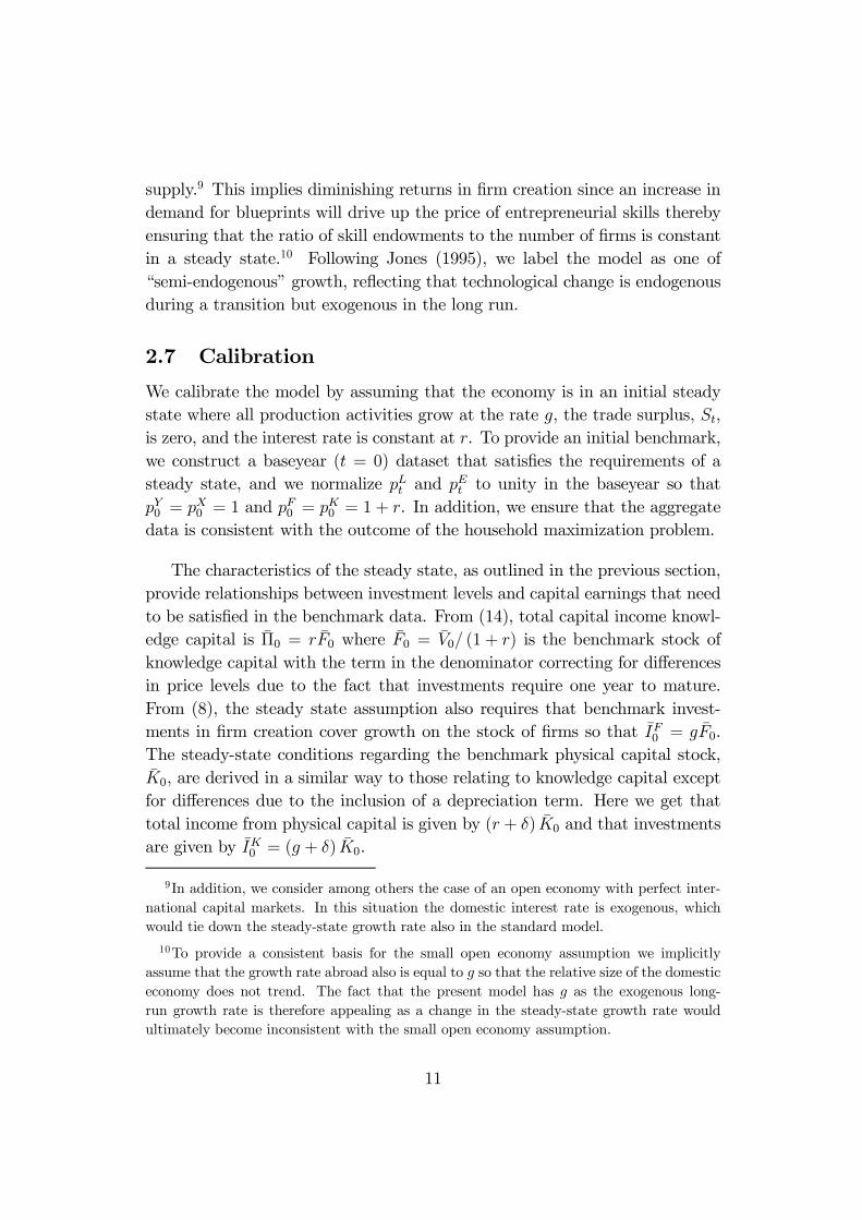
Baltic states in 1998: In Lithuania, for example, of those aged 30 and below,44 percent worked in new enterprises, whereas this was only the case 17 per-cent of those aged 50 and above. Similarly, in Estonia the average monthlysalary of workers in new enterprises was found to be about 30 percent higherthan the salary of workers in old enterprises. These numbers suggest thatthe young have bene…ted disproportionately from the creation of new privatesector enterprises.

There may be several reasons why old workers are less likely than youngworkers to be employed in a new enterprise. One possibility is that the youngare simply endowed with skills that are most demanded in the process of …rmcreation. Or it may be that people have to acquire these skills, and that thecost/bene…t trade-o¤ of this investment is more favorable to the young. Forexample, Friedberg (2002) …nds strong evidence in support of forward-lookingfactors in the decision to acquire computer skills: the number of years toretirement is shown to be an important determinant, which indicates that …xedcosts play a role in skill acquisition. Acquisition of the “entrepreneurial skills”that are valuable in new …rms may involve a similar element of …xed costs,which would make it less worthwhile for those with few years to retirement.

Against that background, the objective of this paper is to formalize thelinkages between economic transition and intergenerational welfare redistri-bution. Thereby, we should be in a better position to understand why thedi¤erent generational groups would, or would not, be likely to support the on-going reform process. For that purpose we develop a model with overlappinggenerations (OLG) and endogenous technological change through expandingproduct varieties. New …rms are created as a result of investments that relyon the input of entrepreneurial skills. Thus, it is entrepreneurial activity thatdrives economic growth.2 The increase in innovative capability associated withopening of the economy is modeled as an exogenous increase in household en-dowments of entrepreneurial skills. While we make various assumptions aboutwhich generations stand to gain from an increase in entrepreneurial possibili-ties, our base case re‡ects the empirical evidence from the Baltics as alluded

2That entrepreneurs play a crucial role for economic growth in transition economies isstrongly indicated by McMillan and Woodru¤ (2002) who argue that ”the success or failureof a transition economy can be traced in large part to the performance of its entrepreneurs”(p. 154).

2

to above. The central point here is that it seems reasonable to assume thatthe young are more responsible for the surge in innovative capacity than arethe old.

Our model has some similarities with the model used by Fougère andMérette (2000) to look at issues relating to population ageing. A central di¤er-ence is that while their endogenous growth mechanism relies on human capitalaccumulation, ours relies on …rm creation. The process of endogenous tech-nological change is important here for several reasons. First, it is capable ofgenerating the large increase in growth rates that have been observed in sometransition economies. In our model endowments of entrepreneurial skills con-stitute a small but …xed share of long-run output and a small increase in thelevel of these endowments may therefore have substantial e¤ects on the overalleconomy.3 Second, in combination with the OLG framework, the formulationof age-dependent levels of entrepreneurial skills can capture the idea that itis the young and future generations that generate the higher output level–andreceive the awards from doing so. Finally, the assumption that a long-runincrease in productivity is dependent on skill sets that are only fully availableamong young and future generations is consistent with the fact that manytransition economies have been slow to realize the high growth rates that werepredicted for them.

Our analysis generates several interesting results. Overall, we …nd thatan increase in entrepreneurial capacity causes not only a surge in economicactivity, but also a redistribution in favor of future generations. While it iswell-known that a transition to a higher income level may involve an initialperiod of rising inequality, we show that such a transition may in fact imply anabsolute reduction in the welfare of older generations. Unless it is fully o¤set byan immediate jump in investments, an increase in entrepreneurial capacity willtend to be associated with a reduction in the unit price of entrepreneurial skillsand a rise in interest rates. The current old thus su¤er from a higher relativeprice of consumption and experience capital losses on existing assets, but donot live long enough to gain from future increases in productivity. International

3This issue is related to the discussion of the determinants of the magnitude of the e¤ectsof trade liberalization. A standard model with constant returns to scale predicts e¤ects thatare much smaller than is generally thought to be the case. Consequently, several authors,including Rutherford and Tarr (2002), have proposed models for evaluating the e¤ects oftrade liberalization that operate with increasing returns to scale.

3

capital markets are important for this outcome, as they in‡uence the extent towhich higher investments can be …nanced without a¤ecting domestic prices andinterest rates. Thus, with imperfect international capital markets we …nd itpossible for a majority of current generations to experience an absolute welfareloss.4 From a political economy perspective this is an important insight, as ito¤ers a plausible explanation for the reluctance to embrace reform agendas intransition economies.

From here the paper proceeds in two main parts. Section 2 presents themodel in detail, including a characterization of the steady state and an outlineof the calibration method. Section 3 then o¤ers an analysis of the e¤ects ofan increase in entrepreneurial capacity, including a discussion of the role ofcapital mobility and other kinds of sensitivity analysis. Section 4 concludes.

2 The model

We work with an overlapping generations model in which economic growthis due to expanding product varieties. In this model, the development ofnew product varieties relies on the use of entrepreneurial skills. In later sec-tions of the paper we use the model to look at the intergenerational e¤ects ofan exogenous increase in entrepreneurial skills, re‡ecting the introduction ofentrepreneur-driven capitalism that characterizes transition economies and isassociated with a process of converging to a higher income level. The modelis deterministic and consumers and …rms have perfect foresight, so investmentdecisions are determined by the time paths of future prices. Final goods areproduced using intermediate inputs, are traded on world markets, and, with-out restrictions on the trade balance, a small open economy assumption meansthat the price is given from abroad. Firms producing intermediate inputs havea monopoly on their particular variety, and new …rms enter if the present value

4Our results rely on a formulation in which households only care about their own life-time consumption. If, alternatively, generations are altruistically linked consumption lossesexperienced by the old would be compensated by the gains expected for future generations.Studies of the advanced economies tend to …nd little or no evidence that such intergener-ational links play an important role, see, e.g., Altonji, Hayashi and Kotliko¤ (1992, 1997).This possibility may nevertheless play a part in explaining the willingness of older genera-tions to su¤er the adverse distributional e¤ects of the transition process. If so, our resultsmay be interpreted as the direct e¤ect on individual welfare excluding altruism.

4

of markup revenue, equal to the value of the …rm, covers the cost of developinga new …rm.

Investments in …rm creation produce “blueprints” where this term shouldbe interpreted broadly as the result of any kind of pro…t-driven activity thatdevelops new knowledge. Examples are inventions of new products or, moregenerally, anything that contributes to a more productive business environ-ment while also generating income for the developer. The number of inter-mediate …rms in the economy can therefore be interpreted as an index ofproductive knowledge. Similarly, the value of these “blueprints”–in our modelequal to the market value of …rms producing intermediates–is akin to the con-cept of knowledge capital. The focus of this paper is …rm creation takingplace within transition economies and not the mere application of inventionsdeveloped abroad.5 We therefore assume that there is no international marketfor blueprints or intermediate inputs in the model. This is reasonable giventhe broad interpretation of a blueprint applied here, as there are importantnon-tradable elements in what constitutes a productive business environment.Further, it is, arguably, exactly the unleashing of the capacity to apply existinghuman capital more productively that best characterizes transition economies.

The production side of the model builds on the endogenous growth frame-work originating in Romer (1987) and subsequently developed in, e.g., Romer(1990) and Barro and Sala-i-Martin (1996, ch. 6). An important di¤erencefrom the standard endogenous growth framework, however, is the presence ofentrepreneurial skills as an input in the production of blueprints for new …rms.In that respect, the production side of the model is essentially the same as theone presented in Rutherford and Tarr (2002). Entrepreneurial skills are mod-eled as exogenous endowments, which means that the number of intermediate…rms cannot in the long run grow faster than the …xed supply of skills. Anotherimportant di¤erence from most studies in the endogenous growth literature isthat we present numerical simulations that allow us to focus on transitional ef-fects rather than solely on analytically derived characterizations of the steadystate. The demand side of the model comprises overlapping generations withperfect foresight along the lines of Auerbach and Kotliko¤ (1987) and Altig,

5Markusen, Rutherford, and Tarr (2001) consider the e¤ects of knowledge imports bypresenting a model of expanding product varieties with both domestic and foreign varietiesof intermediates.

5

Auerbach, Kotliko¤, Smetters, and Walliser (2001). We now turn to a moredetailed description of each of the model’s building blocks.

2.1 Consumer behavior

Final consumption arises from overlapping generations of …nitely-lived house-holds. A household of generation j enters the economy at age 20, retires whenreaching age 60, and is identi…ed by the year t in which it enters the economy.For t = 0; 1; 2; :::, each household maximizes the utility of lifetime consumptionsubject to the budget constraint that the present value of lifetime consumptiondoes not exceed the present value of income:

maxcj;t

u(cj;t) =

j+39Xt=j

µ1

1 + ½

¶t¡j c1¡µj;t

1¡ µ ; (1)

s:t:

j+39Xt=j

pYt cj;t ·j+39Xt=j

¡pLt !

Lj;t + p

Et !

Ej;t

¢+ pF0

¹fj;0 + pK0¹kj;0;

where ½ is the utility discount rate, 1=µ is the intertemporal elasticity of sub-stitution, cj;t is consumption of the …nal good, !Lj;t and !

Ej;t are endowments of

labor and entrepreneurial skills, ¹fj;0 and ¹kj;0 are the exogenously given initialholdings of knowledge capital and physical capital, and the p’s are the corre-sponding present value prices.6 We normalize the world market price of …nalgoods to unity in future value, but domestic prices may di¤er due to changesin the exchange rate, which would then be re‡ected in the domestic inter-est rate. Consequently, in present value terms, pYt =

Qts=1 (1 + rs)

¡1, wherert = p

Yt¡1=p

Yt ¡1 is the interest rate in period t and where pY0 is the numeraire.

Each generation is endowed with both labor and entrepreneurial skills.For simplicity, we assume that the time pro…le of these endowments is ‡atover the life cycle. Furthermore, the aggregate labor supply is constant, soLt =

Pj !

Lj;t = Lt = ¹L 8 t. Entrepreneurial skills, in contrast, are subject to

exogenous growth, making this is the source of long-run economic development.In the baseline, each generations’ endowment of entrepreneurial skills is higherthan the previous generations’ by a factor g so

Pj !

Ej;t = ¹Et = ¹E0 (1 + g)

t. It isagainst this that we compare the e¤ects of a surge in the level of entrepreneurialcapacity.

6Throughout the paper, we express all prices in present value prices relative to time t = 0,and use bars to indicate quantity levels in the baseline.

6

2.2 Final good production

In each year t, the production of the …nal good, Yt, takes place under perfectcompetition using inputs of labor and di¤erentiated intermediate inputs, xi:

Yt = ÁY ¹L1¡®

NtXi=1

x®i;t;

where ÁY = ®¡® (1¡ ®)¡(1¡®) is a scaling parameter, ® is the cost share ofintermediate inputs, and Nt is the number of intermediate …rms at time t,which is proportional to the number of blueprints in the economy. The numberof intermediate …rms is taken as given in the production decision implying thatthere is constant return to scale from the producer perspective, while totalfactor productivity is increasing with Nt overall.

With symmetric …rms, each intermediate …rm produces the same quantityxi;t = xt, and the model may therefore conveniently be formulated in terms ofthe total number of intermediates:

Yt = ÁYN1¡®t

¹L1¡®X®t ;

where Xt= N txt is the aggregate output of intermediates. The aggregate levelof labor endowments is constant at ¹L and total input demands are given by

Xt = Nt

µÁY ®

pYtpXt

¶ 11¡®

¹L; (2)

¹L = (1¡ ®) pYt

pLtYt; (3)

where pXt is the price of intermediates, and the price of …nal goods is given by

pYt = N®¡1t

¡pXt¢® ¡

pLt¢1¡®

: (4)

2.3 Intermediate goods production

Firms produce intermediate output under monopolistic competition with vari-able costs resulting from inputs of …nal goods and physical capital. The sym-metry assumption implies that all …rms producing intermediates have the sametechnology, produce the same level of output, and charge the same price. Con-sequently, total output of intermediates may be expressed in terms of totalinputs:

Xt = ÁXK»tD

1¡»t ; (5)

7

where ÁX = ®¡1 (r + ±)» »¡» (1¡ »)¡(1¡»), r is the baseline interest rate, ± is

the depreciation rate of physical capital, » is the cost share of physical capitalservices, Kt is the stock of physical capital, and Dt are material inputs to theproduction of intermediates. The pro…t maximizing mark-up on the unit costof production is 1=®, so aggregate gross pro…t is ¦t = (1¡ ®) pXt Xt and themarket price of intermediates is

pXt =¡pRKt

¢» ¡pYt¢1¡»

; (6)

where pRKt is the price of physical capital services.

In addition to the variable cost of production, …rms producing intermedi-ates pay a …xed one-time fee for a blueprint, pFt , allowing the …rm to operatein perpetuity. The total equity of such …rms, i.e., the value of all intermediate-producing …rms, is equal to the present value of future pro…ts:

Vt = Nt

1Xs=t

(1¡ ®) pXs xs: (7)

This amount, Vt, may reasonably be interpreted as the knowledge capital ofthe economy.

2.4 Firm creation and capital accumulation

Investment takes place under perfect competition and the two types of capitalaccumulate according to standard convention. In the case of knowledge capital,investments require inputs of …nal goods, Bt, and entrepreneurial skills, Et:

Ft+1 = Ft + ÁNB°t E

1¡°t ; (8)

where ÁN = °¡° (1¡ °)¡(1¡°) and IFt = ÁNB°t E1¡°t is total investment in …rm

creation. We think of each new unit of knowledge capital as a blueprint with aprice pFt , and normalize the number of intermediate-producing …rms to unityin the benchmark so that Nt ¹F0 = Ft meaning that the establishment of anew …rm requires ¹F0 blueprints. With free entry and exit among producersof intermediates, the value of knowledge capital, as expressed in (7), is on themargin equal to the cost of …rm creation so Vt = pFt Ft. Competitive behavioramong investors means that the price of a blueprint, pFt , is equal to the resalevalue plus the rate of return, pRFt :

pFt = pFt+1 + p

RFt : (9)

8

Here cost minimization implies7

pFt+1 =¡pYt¢° ¡

pEt¢1¡°

; (10)

where pEt is the price of entrepreneurial skills and the return on a blueprint isthe monopoly pro…t from a unit of knowledge capital so pRFt = (1¡ ®) pXt Xt=Ft.Investment in physical capital only involves input of …nal goods and a

constant depreciation rate ± applies:

Kt+1 = (1¡ ±)Kt + IKt ; (11)

where IKt is gross investment in physical capital. Competitive behavior impliesthat the price of physical capital is given by

pKt = (1¡ ±) pKt+1 + (r + ±) pRKt ; (12)

where pKt+1 = pYt , and p

RKt = (rt + ±) p

Yt = (r + ±). Here, to simplify the exposi-

tion, we have normalized the rental price of physical capital so pRKt =pYt is equalto unity in the baseline, where r is the baseline interest rate. In a determinis-tic framework arbitrage between the two means of storing value implies thatknowledge capital and physical capital earn the same rate of return measuredin units of a common good.

2.5 Market clearance

Market clearance in the …nal goods market requires supply/demand balance atthe aggregate level as well as consistency with individual household demand:

Yt = Ct +Dt +Bt + IKt + St: (13)

whereP

j cj;t = Ct is the aggregate consumption level and St is the tradesurplus. With the small open economy assumption, the absence of restrictionson trade or international capital mobility means that pYt is given and …xes theeconomy’s interest rate at the rate r that applies on the world market. Whenthe economy cannot access international credit markets the domestic interestrate is endogenous and St = 0.

7This assumes that an equilibrium always involves positive investment levels, which is thecase for all the simulations under consideration. Corner solutions, in which (9) is replaced byan inequality exhibiting complementary slackness with IFt ¸ 0 are, however, accommodatedin our computational framework.

9

2.6 The steady state

To characterize the steady state, consider a given steady state interest rateequal to ~r so pYt = (1 + ~r)¡t, which from the de…nition of pRKt means thatpRKt =pYt is constant. From (6) we get that also pXt =p

Yt is constant, and, conse-

quently, from (2), (3), (4), (5), (8), and (11) we get gX = gN , g(pL=pY ) = gY ,gN = g(pL=pY ), gX = gD = gK, gF = gIF = gB = g, and gK = gIK , where theg’s indicate steady-state growth rates of the term in subscript. Since gF = gNby de…nition, combining these equations shows that all these growth rates arethe same and equal to g, the growth rate in entrepreneurial skills. Given thesegrowth rates, the market clearing condition (13) implies that g = gC = gS andhence we …nd that the steady-state growth rate of all components of productionand consumption are exogenously given.8

To derive the steady-state value of knowledge capital, note that (2) and aconstant pXt =p

Yt implies that the individual …rms’ output of intermediates is

constant so xt = x. From (7), and pXt+i = pXt (1 + ~r)

¡i the total present valueof knowledge capital at time t is then given by

Vt = Nt

1Xs=t

(1¡ ®) pXs x =1 + ~r

~r¦t: (14)

From Vt = pFt Ft andNt = Ft= ¹F0 it follows that pFt =p

Xt and p

Ft =p

Yt are constant.

Finally, from (9) and the expressions for pFt+1 and pRKt we conclude that pEt =p

Yt

is also constant. This means that total household income from entrepreneurialskills grows at the rate g, just as is the case for labor income. Inspection of thevarious price de…nitions shows that all other future-value prices are constant.

That the long-run growth rate in this model is exogenous di¤ers from thestandard expanding product varieties endogenous growth framework in whichlong-run growth is not tied down by the level of endowments but may bea¤ected by policy. The di¤erent outcome follows from our assumption that° < 1 so that investments in …rm creation in (8) involve an input that is in …xed

8The model exhibits the same feature if we include exogenous growth in Lt. In that casegN = g as here, but the model would also involve several other (exogenous) steady-stategrowth rates. To keep the analysis transparent, we keep Lt constant and focus on the engineof growth: e¤ective increases in entrepreneurial capacity.

10

supply.9 This implies diminishing returns in …rm creation since an increase indemand for blueprints will drive up the price of entrepreneurial skills therebyensuring that the ratio of skill endowments to the number of …rms is constantin a steady state.10 Following Jones (1995), we label the model as one of“semi-endogenous” growth, re‡ecting that technological change is endogenousduring a transition but exogenous in the long run.

2.7 Calibration

We calibrate the model by assuming that the economy is in an initial steadystate where all production activities grow at the rate g, the trade surplus, St,is zero, and the interest rate is constant at r. To provide an initial benchmark,we construct a baseyear (t = 0) dataset that satis…es the requirements of asteady state, and we normalize pLt and p

Et to unity in the baseyear so that

pY0 = pX0 = 1 and p

F0 = p

K0 = 1 + r. In addition, we ensure that the aggregate

data is consistent with the outcome of the household maximization problem.

The characteristics of the steady state, as outlined in the previous section,provide relationships between investment levels and capital earnings that needto be satis…ed in the benchmark data. From (14), total capital income knowl-edge capital is ¹¦0 = r ¹F0 where ¹F0 = ¹V0= (1 + r) is the benchmark stock ofknowledge capital with the term in the denominator correcting for di¤erencesin price levels due to the fact that investments require one year to mature.From (8), the steady state assumption also requires that benchmark invest-ments in …rm creation cover growth on the stock of …rms so that ¹IF0 = g ¹F0.The steady-state conditions regarding the benchmark physical capital stock,¹K0, are derived in a similar way to those relating to knowledge capital exceptfor di¤erences due to the inclusion of a depreciation term. Here we get thattotal income from physical capital is given by (r + ±) ¹K0 and that investmentsare given by ¹IK0 = (g + ±) ¹K0.

9In addition, we consider among others the case of an open economy with perfect inter-national capital markets. In this situation the domestic interest rate is exogenous, whichwould tie down the steady-state growth rate also in the standard model.

10To provide a consistent basis for the small open economy assumption we implicitlyassume that the growth rate abroad also is equal to g so that the relative size of the domesticeconomy does not trend. The fact that the present model has g as the exogenous long-run growth rate is therefore appealing as a change in the steady-state growth rate wouldultimately become inconsistent with the small open economy assumption.

11

To ensure that the aggregate data is consistent with the outcome of utilitymaximizing households, we follow the methodology laid out by Rasmussenand Rutherford (2002), which implies calibrating the utility discount rate ½so that

Pj¹fj;0 +

Pj¹kj;0 = ¹F + ¹K. For the numerical simulations presented

in the following, we adopt the parameter values presented in Table A.1., andthe corresponding social accounting matrix shown in Table A.2. This implies½ = 0:003 and the income/consumption pro…les shown in Figure 1, whereendowment income consists of income from sale of labor and entrepreneurialskills.11

Figure 1 about here

Given the ‡at pro…le of endowment income, the model implies a constantbaseline growth rate of consumption over the life cycle. Households accumulateassets during middle age and then dissave when old, as predicted by the life-cycle view of savings.12 Since knowledge capital and physical capital earn thesame net rate of return households are indi¤erent between the two types ofassets. To assign values to ¹fj;0 and ¹kj;0 we therefore assume that all householdshold the two asset types in the same proportion at all times in the initial steadystate.13

The numerical model is formulated over a 200-year horizon and solved inone-year intervals, thus capturing 40 overlapping generations at any point intime. The solution procedure involves imposing a number of terminal con-straints on the model to ensure that the outcome approximates the in…nite

11Consistency could also be achieved by setting ½ exogenously and calibrating either g orr. We choose to calibrate ½ as we view this parameter as the most uncertain. The resultingvalue of ½ = 0:003 is in any case similar to the value of 0.004 used in Altig, Auerbach,Kotliko¤, Smetters, and Walliser (2001) where this parameter is set exogenously.

12The calibrated consumption growth path is somewhat steep through the lifecycle. Amore realistic consumption pro…le could be obtained by imposing a more probable hump-shaped pro…le for e¤ective labor endowments, as it is done in, e.g., Auerbach and Kotliko¤(1987). We abstain from doing so to maintain simplicity.

13This assumption is important as it determines how di¤erent age groups are exposed tocapital gains and losses resulting from changing asset prices due to an unanticipated policychange.

12

horizon equilibrium path to the new steady-state equilibrium (see Rasmussenand Rutherford (2002) for details).14

3 Model results

Based on the rapid growth in new …rms, we think of the reform process intransition economies as closely related to the level of entrepreneurial capacity.Better opportunities for establishing and protecting property rights in thesecountries mean that entrepreneurs are more willing to undertake investments.Also, the greater integration into world markets that follows from market lib-eralization can reasonably be assumed to imply greater opportunities for dis-semination of knowledge. In particular, entrepreneurs may more easily adoptforeign knowledge about how …rm creation is most e¤ectively carried out. Thebottom line is that these countries have experienced a change of circumstancesthat have boosted …rm creation, and we capture this e¤ect in reduced form bya shock to the model that increases the overall level of entrepreneurial skills,Et =

Pj !

Ej;t. We then investigate the distributional consequences of how

increases !Ej;t are distributed among the di¤erent generations.

Table 1 about here

Table 1 shows the proportion of workers in the Baltic countries employedin enterprises established since the transition process began around 1988, asreported by Antila and Ylöstalo (1999). Two features stand out. First, afterjust a single decade a very large part of the workforce is now employed innew …rms. Second, workers in new …rms tend to be young. These results arecomplemented by other …gures also reported by Antila and Ylöstalo, whichshow that average salaries in the Baltic countries are substantially higher innew enterprises than they are in the rest of the economy, and that within newenterprises younger workers earn substantially higher wages than older workers

14The model is programmed in gams/mpsge and solved with the gams/path algorithm(see Rutherford (1999) and Ferris and Munson (2000)), and it is available from the authorsupon request.

13

relative to what is the case in the rest of the economy.15 Estonia, which hasbeen the most successful of the three transition economies, also presents themost extreme example. Here, average wages in new enterprises are about 30percent higher than the rest of the economy, and within new enterprises theunder 30-year-olds earn about 30 percent more than those over 50 while thetwo age groups earn about the same in the rest of the economy. All this pointsto a clear picture of developments that have favored younger workers.

One likely explanation for these developments is that younger workers havebene…ted by having a better match with the skills that are most valuable inthe new business environment. Presumably, younger workers are more inclined,and perhaps more able, to attain the set of skills–ranging from computer skillsto entrepreneurship–that have become especially valuable. Even if the abilityto obtain such new skills is the same, older generations have a shorter remain-ing life span and are therefore may be reluctant to undertake the investmentin acquiring these skills.16 While such considerations are probably true every-where, they are especially important in transition economies where economicrestructuring has suddenly introduced a wide disparity between the existingskill-base and the demands of the workplace.

To capture the relationship between the transition process, seen here as theforces accompanying an increase in …rm creation, and the advantage of beingyoung, we use the data in the last column of Table 1 to formulate the balticscenario. In this transition path generations who enter the economy in year 0 oranytime thereafter experience a proportional increase of their entrepreneurialendowment, !Ej;t, by ¯ so that Et = (1+¯) ¹Et for t ¸ 39. Generations with ages21 to 30 in year 0, in contrast, experience a smaller increase of 0:80¯; thosebetween ages 40 and 31 experience an increase of 0:62¯; those between ages 50and 41 experience an increase of 0:46¯; and those older than 51 experience nogain at all. This implies that in year t = 10 the increase in skill endowmentsaccruing to the di¤erent generations will be distributed in accordance withthe Baltic age pro…le of workers in new …rms. As such this is a simpli…edway of re‡ecting the observed bene…ts of being young in a model that does

15In this data, Latvia is an exception in that the age pro…le of wages in new enterprisesis not signi…cantly di¤erent from that in the rest of the economy, although average salariesin new enterprises are higher also in this country.16Friedberg (2002) …nds such an e¤ect in acquisition of computer skills in the U.S. where

evidence suggests that computer use is associated with a lower probability of retirement.

14

not distinguish between di¤erent types of skills or labor. In our numericalcalculations we investigate transition paths associated with ¯ = 0:1, i.e., anincrease in the long-run level of entrepreneurial skills of 10 percent.

Obviously, this approach represents only one of many possible interpreta-tions of the underlying causes for the developments summarized by the datain Table 1. For example, the relative disadvantage experienced by the old maysimply re‡ect that uncompetitive wage setting in favor of the old is more preva-lent in old enterprises. To put perspective on the importance of the speci…cdetails of the shock that is imposed on the model, we consider two alternativescenarios: uniform and young that bracket the range of possible allocationsof skill increases between the young and the old. In the uniform scenarioall generations share the same proportional increase in entrepreneurial endow-ments. In the young scenario only new generations, i.e., those entering theeconomy after year 0, bene…t. These two extreme cases would correspond to asituation where acquisition of entrepreneurial skills is entirely determined byan investment decision, and where the …xed cost of skill acquisition in one caseis so small that all generations undertake the investment, while the cost in theother case is so large that only new generations do.17

Since neither of the three shocks change the steady-state growth rate ofEt, the resulting steady state may be compared to the baseline by noting thatthis is equivalent to a simple re-scaling of the units in the model so that pLt =p

Et

increases by ¯. Consequently, all components of household income increaseby the same amount and there is no change in the steady-state interest rate.Using the logic of Section 2.6 we know that all aggregate production activities,as well as pLt =p

Yt , will continue to have a steady state growth rate equal to g,

while pXt =pYt and all other relative prices except those relating to p

Lt return to

the baseline level. As a result, aggregate consumption and all output level willalso increase by ¯, and from (13), this implies that the trade balance will returnto zero. The di¤erent shocks thus all have the same steady state impact, but,as we show in the next section, the transitional dynamics will di¤er markedly.

17With the Cobb Douglas technology in (8), the case where all generations bene…t soEt = (1 + ¯) ¹Et for 8 t ¸ 0 is equivalent to a situation with a one-time increase in the totalfactor productivity of …rm creation. This situation may also be interpreted as one wherebetter property rights make resources used for …rm creation more productive.

15

3.1 Transitional dynamics

When the model is exposed to a shock it will undergo a transition to a newsteady state. Investments in physical capital accumulation only require inputsof …nal goods, which are traded on the world market. With no restrictions onthe trade balance, the small open economy assumption means that the supplyof inputs to physical capital investments is perfectly elastic. Consequently,the economy would adjust immediately to a shock that only a¤ects the phys-ical capital stock and the interest rate would remain constant. In contrast,the shocks that we consider here involve the level of entrepreneurial capacity,which impacts on the steady-state number of …rms. Because one of the inputsto investment in …rm creation, entrepreneurial skills, is in …xed supply cost-minimization dictates that investments will only gradually bring the numberof …rms to the new steady-state level even if the interest rate is una¤ected.

The absence of credit markets has important implications for transitionaldynamics. A binding restriction on the level of the trade de…cit means that theeconomy cannot rely on imports to immediately adjust to a shock, but wouldadjust its exchange rate to match imports with exports. In such a situation,an increase in investments in …rm creation following from a shock to Et will bespread out over a number of years and the domestic interest rate changes overthe transition.18 Eventually, however, the model will reach the new steadystate where the interest rate has returned to r and all relative prices, exceptthose relating to pLt , will have returned to the initial level. Intuitively, to theextent that the increase in potential income in transition economies is relatedto an increase in stocks of knowledge or physical capital that are costly tobuild up too rapidly, it makes sense that it does not happen immediately.

3.1.1 Perfect capital mobility

We …rst consider a situation where there are no restrictions on the economy’sability to borrow abroad to …nance a temporary trade de…cit other than thatthe present value of exports must equal the present value of imports overthe in…nite horizon. Figure 2 shows the impact over the …rst part of thetransition following from the shock to Et. This situation implies an initial

18An extreme example of such a trade restriction would be to allow no trade whatsoever,in which case the model would simply be one of a closed economy.

16

de…cit as investors exploit the opportunity to …nance part of the initial increaseof investments in …rm creation on the world capital market.

Figure 2 about here

Since the interest rate and the price of …nal goods are in this setting givenby the level on the world market, pXt and p

Yt are both …xed at the baseline level.

From (2) we then get that xt = x, and we can follow the approach of Section2.6 to conclude that pFt and p

Et also are …xed at the baseline level. This implies

that all prices are unchanged except pLt , which by (3) grows over time at thesame rate as output, Yt, where also gYt = gNt. The evolution in the number of…rms, Nt, is consequently the driving force of the transitional dynamics. Pro…tmaximization means that investments in …rm creation are carried out up tothe point where the cost, as implied by (9), is equal to income as de…ned by(7). Since there is no depreciation of knowledge capital and both input andoutput prices of investments in …rm creation are unchanged, it follows from(8) that the level of these investments is proportional to Et.

Consider …rst the uniform scenario in which all generations bene…t fromthe productivity increase. Here Et = (1 + ¯) ¹Et 8 t ¸ 0 and IFt jumps im-mediately to the new steady state level, i.e., an increase by ¯. We can thenquantify the speed of the transition by noting that the actual number of …rms,Nt, is given by

Nt ¹F0 = ¹IF0 =g +t¡1Xs=0

(1 + ¯)¹IF0 (1 + g)s ;

which di¤ers from the steady-state level, N¤t , given by

N¤t¹F0 = (1 + ¯)¹I

F0 =g +

t¡1Xs=0

(1 + ¯)¹IF0 (1 + g)s = (1 + ¯)¹IF0 (1 + g)

t =g:

De…ning the speed of transition as the rate of change in ¹t, where ¹t =(N¤

t ¡Nt) =N¤t is the fraction of the remaining di¤erence from the steady state

number of …rms that vanishes in year t, we get ¹t = (1 + g)¡t ¯=(1 + ¯). In

other words, the speed of the transition is constant and equal to g. With a

17

2 percent annual growth rate in the steady state, this means that it takes 35years for the number of …rms to reach half of the long-run increase. In thebaltic and young scenarios Et only approaches the new steady state levelgradually and does not reach (1 + ¯) ¹Et until all generations in the economyare of the type that have bene…ted from the full productivity increase, whichhappens in year 39. Consequently, investments are initially lower and Nt, andhence also pLt and Yt, take longer to reach the new steady state level.

With all prices except pLt unchanged, the continuous increase in the numberof …rms means that all generations bene…t from the shock. Every generationentering the economy after year 0, as well as those of the current generationsthat are assumed to bene…t from higher endowment levels, experience a levelincrease in earnings from the sale of entrepreneurial skills. Over time eachgeneration that lives past year 0 also experiences increasing labor income dueto the rise in pLt . This produces the welfare gains shown in Panel A, where theequivalent variation ultimately levels o¤ at 10 percent corresponding to thelong-run increase in household income.19 ;20

With all generations experiencing an increase in life-cycle income, the shockcauses a jump in aggregate consumption, Ct. Output, Yt, on the other hand,is only growing gradually at the rate gNt , which, as shown in Panel B, meansa large initial trade de…cit when all generations experience the increase in en-trepreneurial skill earnings, but a smaller trade de…cit when household incomeis increasing more gradually as is the case when only new generations expe-rience the increase in entrepreneurial skill earnings. Subsequently, the tradebalance improves as household income grows at a slower rate than output,with the ratios Ct=Yt showing the inverse relationships of those appearing inPanel B. After a period with de…cits, the trade balance thus becomes positive,allowing debt incurred during the initial part of the transition to be paid back,and eventually the balance returns to zero.

19For the initial population the reported welfare changes relate to remaining life timeutility.

20To evaluate the signi…cance of the OLG demand system, it is useful to compare these re-sults to those arising with an Ramsey-type characterization of household demand. Assuminga single in…nitely-lived agent with an utility discount rate equal to (1 + r) = (1 + g)µ¡1 andotherwise maintaining the above parameterization produces the same baseline equilibrium.Here a 10 percent increase in this agents endowment of entrepreneurial skills results in anequivalent variation of 3.8 percent.

18

3.1.2 Imperfect capital mobility

We now consider a situation where trade is required to balance in every year,i.e., St = 0, and Figure 3 shows the results. As shown above, the long runimpact is the same as in the situation without any restrictions on the tradebalance. In contrast to that situation, however, pYt is no longer declining witha constant interest rate so all relative prices, not just those relating to pLt , arechanging during the transition. Without the possibility of using internationalcapital markets to …nance a temporary trade de…cit, the immediate increasein investments in …rm creation is smaller than before, implying a slower tran-sition. As shown in Panel A, in the uniform scenario it takes 40 years forthe number of …rms to reach half of the steady state increase, and, at theother extreme in the young scenario, the same adjustment takes almost 60years. Now the initial increase in investments requires households to foregoconsumption so that Ct=Yt must fall rather than increase as it did in the pre-vious case. From Panel B we see that these ratios are in all cases initiallydecreasing, re‡ecting gradually rising investment ratios. This contrasts to thesituation without the restriction on the trade balance where the impact on theCt=Yt ratio was positive in the …rst part of the transition.

Figure 3 about here

The changes in investment levels are accompanied by the developmentsin the relative prices shown in Panels C and D. From (8) and (10) we getthat Et = (1¡ °)

¡pYt =p

Et

¢°IFt . Hence, because the increase in entrepreneurial

capacity is not o¤set by a correspondingly large jump in investments there is aninitial reduction in pEt =p

Yt , where, in each of the three scenarios, the magnitude

of the initial decline re‡ects the magnitude of the increase in Et and is lessthan (1+¯). In subsequent years, the decline is in all cases reversed as IFt rises.The e¤ect on income is thus positive for generations that experience the fullincrease in skills but negative for those who are una¤ected. The relative price oflabor, pLt =p

Yt , like that of entrepreneurial skills, is also lower than in the case

with perfect capital mobility re‡ecting the smaller number of intermediate-producing …rms. Consequently, total household income from these two sourcesis growing more slowly than before.

19

As shown in Panel E, the shocks have a positive impact on the interestrate, which re‡ects the increasing demand for investments. In the youngscenario the interest rate is falling for the …rst few years. This is the result ofthe negative e¤ect on income of the decline in pEt =p

Yt for generations living in

the initial years, which causes an increase in the supply of savings that morethan o¤sets the e¤ect of increased investments. Inspecting (1) we note thatthe expression for total present value income appearing on the r.h.s. of thebudget constraint may be rewritten as

j+AXt=j

tYs=1

(1 + rs)¡1µpLtpYt!Lj;t +

pEtpYt!Ej;t

¶+ pF0

¹fj;0 + pK0¹kj;0:

This expression allows us to distinguish income changes due to the changes infuture value prices from those due to changes in the interest rate. The mostlypositive impact on interest rates tends to be welfare-worsening for the youngwho, as seen from Figure 1, are net borrowers, while the impact is positive forthe old who are net lenders.

The …nal source of income changes for generations living in year 0 is achange in pF0 and p

K0 , i.e. changes in the value of assets held at the time of the

shock. From (5) and cost minimizing behavior we get that

Xt =(r + ±)Kt

®»

·pXtpYt

¸ 1¡»»

:

Substituting this expression into (2) and noting that K0, N0, and pY0 (thenumeraire) are all unchanged from the benchmark, we get that also pX0 andhence X0 are unchanged. Equation (6) implies that pXt =p

Yt =

¡pRKt =pYt

¢»so

that pRK0 is also una¤ected by the shock. From (12) and pKt+1 = pYt thismeans that the same is true for pK0 . The only welfare e¤ect on account ofan initial change in asset values is therefore the change in pF0 . Since p

RFt =

(1¡ ®) pXt Xt=Ft the shock has no e¤ect on pRF0 , and from (9) and pFt+1 =¡pYt¢° ¡

pEt¢1¡°

we then get that the change in the price of knowledge capital is

given by 4pF0 =¡pE0¢1¡° ¡ 1. Consequently, the …rst period reduction in the

price of entrepreneurial skills is followed by a somewhat smaller reduction inthe price of knowledge capital. In e¤ect, a reduction in the cost of innovationcauses a fall in the unit value of existing knowledge, which imposes capitallosses on older generations.

20

The changes in incomes of the di¤erent generations are re‡ected in thewelfare changes shown in Panel F. The simulations show that in all scenariosthe change in income of the oldest generation due to the reduction in pF0 isof an order of magnitude greater than income changes due to other sourcesre‡ecting that older generations bene…t little from rising wages and that thechange in interest rates is small. Consequently, the oldest generation in allcases ends up with the largest welfare loss. On the other hand, the youngestgenerations living in year 0 all experience a welfare gain. These generationshave small asset holdings, and as a result they are not much a¤ected by thedecline in pF0 and they also bene…t more by living further into the years withrising wages.21

The negative impact of capital losses is particularly great in the uniformscenario since this case also implies the greatest increase in E0. Here, the oldestgeneration experiences a welfare loss of almost 1 percent, i.e. nearly 10 percentof the long run increase in welfare, and losses apply to all households olderthan 49 years of age. At the other extreme, in the young scenarios (whenonly new generations bene…t) capital losses are smaller, but here the e¤ecton entrepreneurial skill earnings is increasingly negative so that the welfareloss is smaller initially but extends to all households older than 37. In theintermediate case based on the Baltic experience the cut-o¤ age is 46, whichmeans that 35 percent of the initial population becomes worse o¤.

3.2 Sensitivity analysis

Table 2 shows the implications of the productivity shock with alternative pa-rameter values in the case with yearly trade balance restrictions. Using a lowervalue of the intertemporal elasticity of substitution, 1=µ, of 0.4 does not af-fect aggregate quantities in the baseline, but implies that households desire ahigher degree of consumption smoothing. Consequently, equivalent variationsdecline during the transition, as households are more adverse to the changingrelative prices that follow from the shock. The negative welfare e¤ect increasesthe share of the initial population that experiences a welfare loss.

21In this case, the Ramsey-type characterization of household demand results in an equiv-alent variation of 3.2 percent.

21

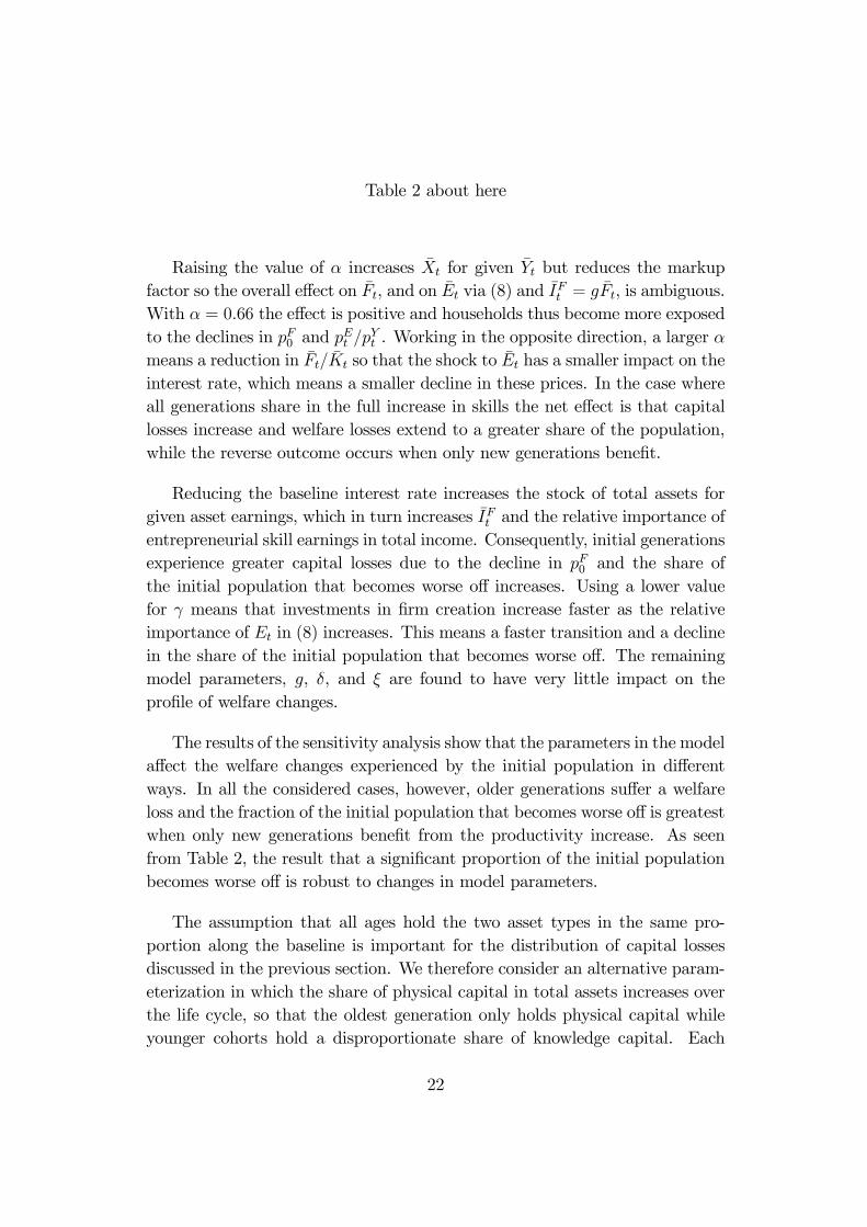
Table 2 about here

Raising the value of ® increases ¹Xt for given ¹Yt but reduces the markupfactor so the overall e¤ect on ¹Ft, and on ¹Et via (8) and ¹IFt = g ¹Ft, is ambiguous.With ® = 0:66 the e¤ect is positive and households thus become more exposedto the declines in pF0 and p

Et =p

Yt . Working in the opposite direction, a larger ®

means a reduction in ¹Ft= ¹Kt so that the shock to ¹Et has a smaller impact on theinterest rate, which means a smaller decline in these prices. In the case whereall generations share in the full increase in skills the net e¤ect is that capitallosses increase and welfare losses extend to a greater share of the population,while the reverse outcome occurs when only new generations bene…t.

Reducing the baseline interest rate increases the stock of total assets forgiven asset earnings, which in turn increases ¹IFt and the relative importance ofentrepreneurial skill earnings in total income. Consequently, initial generationsexperience greater capital losses due to the decline in pF0 and the share ofthe initial population that becomes worse o¤ increases. Using a lower valuefor ° means that investments in …rm creation increase faster as the relativeimportance of Et in (8) increases. This means a faster transition and a declinein the share of the initial population that becomes worse o¤. The remainingmodel parameters, g, ±, and » are found to have very little impact on thepro…le of welfare changes.

The results of the sensitivity analysis show that the parameters in the modela¤ect the welfare changes experienced by the initial population in di¤erentways. In all the considered cases, however, older generations su¤er a welfareloss and the fraction of the initial population that becomes worse o¤ is greatestwhen only new generations bene…t from the productivity increase. As seenfrom Table 2, the result that a signi…cant proportion of the initial populationbecomes worse o¤ is robust to changes in model parameters.

The assumption that all ages hold the two asset types in the same pro-portion along the baseline is important for the distribution of capital lossesdiscussed in the previous section. We therefore consider an alternative param-eterization in which the share of physical capital in total assets increases overthe life cycle, so that the oldest generation only holds physical capital whileyounger cohorts hold a disproportionate share of knowledge capital. Each

22

generation then has a short position in physical capital holdings for approxi-mately the …rst half of the life cycle.22 The decline in pF0 is the major sourcefor the welfare losses of older cohorts, so this alternative formulation reducesthe welfare losses experienced by the old by shifting them to the young, whichcauses the proportion of the initial population that becomes worse o¤ to de-cline. When only new generations experience an increase in entrepreneurialskills, the alternative formulation increases initial holdings of knowledge capi-tal of the pivotal generations around ages 30-40 in year zero, which causes anincrease in the proportion of the initial population, which is adversely a¤ected.

4 Concluding remarks

The transition process from command to market economy in Central and East-ern European countries has been characterized not only by a rapid increasein private sector economic activity, but typically also by worsening welfarefor older generations. In this paper we have presented an overlapping genera-tions model, augmented by endogenous growth operating through expandingproduct varieties, which is capable of generating these two “stylized facts”.

From a methodological perspective, we are not aware of any similar attemptto formalize the rise in private business formation in the context of transitioneconomies. Indeed, the model presented in this paper is notable because aconventional approach with constant returns to scale would fail to account forthe substantial increase in total factor productivity that has been experiencedby most transition economies. Also, we believe that the application of overlap-ping generations of intertemporally optimizing households represents a noveltyin the study of the transition process. More importantly, the combination ofendogenous technological change and an OLG demand system within a uni…ed

22The speci…c formula used to allocate asset holdings is here given by ¹a =

¸p39¡ aPa ¹ma=

Pa ¹ma

p39¡ a, where ¹a is the proportion of total baseline assets held

as knowledge capital at age a, ¹ma is total asset holdings by age, and ¸ = ¹Ft=¡¹Ft + ¹Kt

¢is the proportion of knowledge capital in total assets for the economy as a whole. A for-mulation that further reduces holdings of knowledge capital by the oldest generations, e.g.,by replacing the square root terms in the above expression by a power greater than onehalf, can produce the outcome that no generations experience a welfare loss in the uniformscenario. The baltic and young scenarios result in welfare losses for some generations nomatter what power is used.

23

analytical framework seems to capture two crucial elements of the transitionprocess.

From a policy perspective the conclusion of the paper is quite stark. In-deed, while market reforms are widely regarded as necessary for the creationof prosperity in the medium-to-longer term, they are very likely to be voteddown in a “democratic referendum”. In fact, in some scenarios shown in thepaper, more than half of the working age population is made worse o¤ bywindfall gains from market liberalization that increase long-run consumptionpossibilities. This outcome is possible because an increase in the economy’scapacity to generate new knowledge is likely to reduce the value of existingknowledge, which in‡icts capital losses on the old. As a result, there is adistinct possibility that the outcome of a democratic process would be a voteagainst market liberalization, despite its long-run bene…ts.23 Thus, the mostlikely obstacle to market reforms emerges from an intergenerational con‡ict inobjectives: older generations who bear the burden without reaping the gainsare likely to oppose reform. This may also help explain the apparent realityof life in transition economies where market-oriented reforms have often beenslow to be implemented. This is an interesting property of the model, notleast since many observers seem to have been surprised by the fact that thetransition takes so long time.

In future work we plan to extend the model in several directions. For ex-ample, while economic growth in the current version of the model is drivenby entrepreneurial activity, it would be interesting to allow for endogenousskill (human capital) formation. Also, as a successful implementation of mar-ket reforms would typically require a careful balance between both inter- andintragenerational fairness, we would like to consider a model encompassingseveral di¤erent socioeconomic groups within each generation.

ReferencesAghion, P., and S. Commander (1999): “On the Dynamics of Inequality in theTransition,” Economics of Transition, 7(2), 275–298.

23Jensen and Rutherford (2002) o¤er a similar political economy explanation why publicdebt reduction would almost surely be voted down in a referendum, even though it wouldmost likely be bene…cial from a welfare perspective.

24

Altig, D., A. Auerbach, L. Kotlikoff, K. Smetters, and J. Walliser(2001): “Simulating Fundamental Tax Reform in the United States,” AmericanEconomic Review, 91(3), 574–595.

Altonji, J., F. Hayashi, and L. Kotlikoff (1992): “Is the Extended Family Al-truistically Linked? Direct Tests Using Micro Data,” American Economic Review,82, 1177–1198.

(1997): “Parental Altruism and Inter Vivos Transfers: Theory and Evi-dence,” Journal of Political Economy, 105, 1121–1166.

Antila, J., and P. Ylöstalo (1999): Working Life Barometer in the BalticCountries. Finish Ministry of Labor, Helsinki.

Auerbach, A. J., and L. J. Kotlikoff (1987): Dynamic Fiscal Policy. Cam-bridge University Press, Cambridge, MA.

Barro, R. J., and X. Sala-I-Martin (1995): Economic Growth. McGraw-Hill,New York, NY.

Ferris, M. C., and T. S. Munson (2000): GAMS/PATH User Guide Version4.3GAMS Development Corporporation.

Fischer, S., and R. Sahay (2001): “The Transition Economies After Ten Years,”in Transition and Growth in Post-Communist Countries: The Ten-Year Experi-ence, ed. by L. T. Orlowski. Edward Elgar, Cheltenham.

Fougère, M., and M. Mérette (2000): “Population Aging, IntergenerationalEquity, and Growth: Analysis with an Endogenous Growth Overlapping Genera-tions Model,” in Using Dynamic General Equilibrium Models for Policy Analysis,ed. by G. W. Harrison, S. E. H. Jensen, L. H. Pedersen, and T. F. Rutherford.North-Holland, Amsterdam.

Friedberg, L. (2002): “The Impact of Technological Change on Older Workers:Evidence from Data on Computer Use,” Industrial and Labor Relations Review,to appear.

Jensen, S. E. H., and T. F. Rutherford (2002): “Distributional E¤ects ofFiscal Consolidation,” Scandinavian Journal of Economics, 104(3), 471–493.

Jones, C. I. (1995): “R&D-Based Models of Economic Growth,” Journal of Polit-ical Economy, 103(4), 759–784.

Keane, M. P., and E. S. Prasad (2002): “Inequality, Transfers and Growth:New Evidence from the Economic Transition in Poland,” Review of Economicsand Statistics, to appear.

25

Markusen, J., T. F. Rutherford, and D. G. Tarr (2001): “Foreign DirectInvestments in Services and the Domestic Market for Expertise,” NBERWP 7700,National Bureau of Economic Research, Cambridge, MA.

McMillan, J., and C. Woodruff (2002): “The Central Role of Entrepreneursin Transition Economies,” Journal of Economic Perspectives, 16, 153–170.

Rasmussen, T. N., and T. F. Rutherford (2002): “Modeling OverlappingGenerations in a Complementarity Format,” Journal of Economic Dynamics andControl, to appear.

Romer, P. M. (1987): “Growth Based on Increasing Returns Due to Specializa-tion,” American Economic Review, Papers and Proceedings, 77(2), 56–62.

(1990): “Endogenous Technological Change,” Journal of Political Economy,98(5), S71–S102.

Rutherford, T. F. (1999): “Applied General Equilibrium Modeling with MPSGEas a GAMS Subsystem: An Overview of the Modeling Framework and Syntax,”Computational Economics, 14, 1–46.

Rutherford, T. F., and D. Tarr (2002): “Trade Liberalization, Product Varietyand Growth in a Small Open Economy: A Quantitative Assesment,” Journal ofInternational Economics, 56, 247–272.

26

Appendix

Table A.1. Central Parameter Valuesr Baseline interest rate 0.05

g Baseline growth rate 0.02± Capital depreciation rate 0.101=µ Intertemporal elasticity of substitution 0.80

® Intermediates cost share in …nal good production 0.25» Capital cost share in intermediate good production 0.33

° Final goods cost share in …rm creation 0.33

Table A.2. Benchmark Social Accounting MatrixGoods Sectors Factors Institutions

Y X Y X L E K F C I

Y 4.2 91.7 4.1

X 25

Y 100

X 25

L 75

E 5.0

K 2.1

F 18.8

C 75 5.0 2.1 18.8

I 9.2

Notes: Values scaled so …nal good output = 100. Columns represent expenditures and rows

represent receipts. We assume that there are no imports or exports in the benchmark.

27

Table 1. Proportion of a given age group working in enterprises establishedafter 1988 (%)a

Level Balticsb relative

Age Estonia Latvia Lithuania Balticsb to “Under 30”

Under 30 45 54 44 48 100

30-39 40 39 36 38 80

40-49 32 33 23 29 62

Over 50 29 20 17 22 46

Average 37 37 30 34 72Source: Antila and Ylöstalo (1999) and authors’ own calculations. a1998 share of employed

between ages 16 and 64. bAverage of the three countries.

Table 2. Share of initial population that experiences a welfare loss (%)Scenario

uniform baltic youngBase case 27.5 35.0 57.51=µ = 0:4 35.0 42.5 62.5

® = 0:66 32.5 37.5 55.0r = 0:04 30.0 37.5 60.0

° = 0:1 25.0 32.5 55.0

Alternative distribution of initial assets 17.5 32.5 60.0Notes: Assumes that international trade is balanced in each year. The base case involves

1/µ = 0:8, ® = 0:25, r = 0:05, and ° = 0:33.

Figure 1: Baseline income and consumption profiles

Figure 2: Impact of an increase in the entrepreneurial skills of select genera-tions. International trade balanced intertemporally over the infinite horizon.

Figure 3: Impact of an increase in the entrepreneurial skills of select genera-tions. International trade balanced in each year.