ECONOMIC STUDIES DEPARTMENT OF ECONOMICS SCHOOL OF ... · Kolmannessa esseessä testaan hypoteesia...
104
ECONOMIC STUDIES DEPARTMENT OF ECONOMICS SCHOOL OF ECONOMICS AND COMMERCIAL LAW GÖTEBORG UNIVERSITY 147 _______________________ ESSAYS ON THE POLITICAL ECONOMY OF LAND USE CHANGE Johanna Jussila Hammes ISBN 91-85169-06-4 ISSN 1651-4289 print ISSN 1651-4297 online
Transcript of ECONOMIC STUDIES DEPARTMENT OF ECONOMICS SCHOOL OF ... · Kolmannessa esseessä testaan hypoteesia...

ECONOMIC STUDIES
DEPARTMENT OF ECONOMICS SCHOOL OF ECONOMICS AND COMMERCIAL LAW
GÖTEBORG UNIVERSITY 147
_______________________
ESSAYS ON THE POLITICAL ECONOMY OF LAND USE CHANGE
Johanna Jussila Hammes
ISBN 91-85169-06-4 ISSN 1651-4289 print ISSN 1651-4297 online

Essays on the Political Economy of Land Use
Change
Johanna Jussila Hammes
Department of Economics
Göteborg University
Box 640
S-40530 Göteborg
E-mail: [email protected]
18 November 2005

ii

Contents
Introduction ix
0.1 Related literature . . . . . . . . . . . . . . . . . . . . . . . . . . . xi
0.2 Essay I: Land taxation, lobbies and technological change: internal-
izing environmental externalities . . . . . . . . . . . . . . . . . . . xiv
0.3 Essay II: Agricultural trade liberalization and deforestation: Polit-
ical economy connections? . . . . . . . . . . . . . . . . . . . . . . xv
0.4 Essay III: An empirical examination of land taxation in EU-15 . . xvii
1 Land Taxation, Lobbies and Technological Change: InternalizingEnvironmental Externalities 1
1.1 Introduction . . . . . . . . . . . . . . . . . . . . . . . . . . . . . . 2
1.2 The Model . . . . . . . . . . . . . . . . . . . . . . . . . . . . . . . 5
1.3 The Politically Optimal Tax Rate . . . . . . . . . . . . . . . . . . 9
1.4 Technological Change . . . . . . . . . . . . . . . . . . . . . . . . . 12
1.5 Conclusions . . . . . . . . . . . . . . . . . . . . . . . . . . . . . . 15
1.A Appendix . . . . . . . . . . . . . . . . . . . . . . . . . . . . . . . 19
1.B Appendix . . . . . . . . . . . . . . . . . . . . . . . . . . . . . . . 21
1.C Appendix . . . . . . . . . . . . . . . . . . . . . . . . . . . . . . . 22
1.D Appendix . . . . . . . . . . . . . . . . . . . . . . . . . . . . . . . 23
1.E Appendix . . . . . . . . . . . . . . . . . . . . . . . . . . . . . . . 23
2 Agricultural Trade Liberalization and Deforestation: Political Econ-omy Connections? 25
2.1 Introduction . . . . . . . . . . . . . . . . . . . . . . . . . . . . . . 26
2.2 The Model . . . . . . . . . . . . . . . . . . . . . . . . . . . . . . . 30
2.3 Determination of Equilibrium . . . . . . . . . . . . . . . . . . . . 33
2.3.1 Adjustment of land use . . . . . . . . . . . . . . . . . . . . 33
2.3.2 Determination of the equilibrium tari¤ . . . . . . . . . . . 34
2.3.3 The e¤ect of contributions on tari¤s . . . . . . . . . . . . . 38
2.3.4 The e¤ect of trade liberalization on land allocation . . . . 38
2.4 Extensions . . . . . . . . . . . . . . . . . . . . . . . . . . . . . . . 41
iii

iv2.4.1 Exogenous land subsidy . . . . . . . . . . . . . . . . . . . 41
2.4.2 Co-operative lobbying . . . . . . . . . . . . . . . . . . . . 44
2.5 Conclusions . . . . . . . . . . . . . . . . . . . . . . . . . . . . . . 45
3 An Empirical Examination of Land Taxation in EU-15 513.1 Introduction . . . . . . . . . . . . . . . . . . . . . . . . . . . . . . 52
3.2 The Theoretical Model . . . . . . . . . . . . . . . . . . . . . . . . 55
3.3 Empirical Speci�cation of the Model . . . . . . . . . . . . . . . . 58
3.3.1 Data and Variable Description . . . . . . . . . . . . . . . . 58
3.3.2 Speci�cation of the Equations . . . . . . . . . . . . . . . . 63
3.4 Empirical Results . . . . . . . . . . . . . . . . . . . . . . . . . . . 65
3.4.1 Estimating the Elasticities . . . . . . . . . . . . . . . . . . 65
3.4.2 Estimates for the Land Tax . . . . . . . . . . . . . . . . . 66
3.5 Conclusions . . . . . . . . . . . . . . . . . . . . . . . . . . . . . . 70
3.A Appendix . . . . . . . . . . . . . . . . . . . . . . . . . . . . . . . 76

Acknowledgements
I wish to express my gratitude to my supervisor Thomas Sterner for seeing to the
�nancing of Per Fredriksson�s stay at the University of Gothenburg during 2003.
Per helped me to get started with writing by introducing the Grossman-Helpman
model to me. He also provided valuable comments on the draft versions of the
articles included in this thesis. I am greatly indebted to him for all his support.
Great thanks are also due to the discussant at my licentiate seminar in June
2004, Toke Aidt, and the discussant at my �nal seminar, François Salanie. I also
wish to thank the other people who have made comments on the articles included
in this volume, namely Thomas Sterner, Lennart Flood, Ola Olsson and Klaus
Hammes. Finally, I am grateful to Yves Plees at the EU Commission for answering
my data-related questions and for providing me with some of the data used in the
third essay of the thesis.
I also wish to thank Heather Congdon Fors for the lunches we have enjoyed
together over the past �ve years, and for not taking the side of bullies.
Finally, I am grateful to Klaus Hammes for everything. Without your encour-
agement and support, our discussions, your answers to my stupid questions or
your introduction to panel econometrics, I could never have made it.
Gothenburg, Sweden, May 2005
Johanna Jussila Hammes
v

vi
Till Klaus

viiABSTRACT
This thesis consists of three articles. The two �rst ones construct theoretical modelsfor land use change between agriculture and forestry in the presence of lobbies repre-senting both sectors. The third article tests empirically the hypothesis forwarded in the�rst essay.
In the �rst essay we assume that agricultural land use causes a negative externalityas compared to forestry. The government attempts to internalize this with the help ofa land tax on agriculture. The tax a¤ects the allocation of land between agricultureand forestry. We �nd that in social optimum the government imposes a land tax onagriculture because of the negative externality. In political optimum, if lobby groupsorganize in the agricultural and forestry sectors, their land demand elasticities determinewhether land will be taxed or subsidized. Then, if land demand in agriculture is inelasticenough, land might be subsidized. This is contrary to the received public economicswisdom of taxing goods with low elasticities and constitutes a political economy avenuethrough which the elasticity of land demand a¤ects the tax rate. We further show thatif there is technological progress in agriculture, land demand by agriculture increasesand land demand by forestry falls. Then, it would be socially optimal for the land tax toincrease in technology, but in the political optimum, i.e., if the government is susceptibleto lobbying, the tax rate will rather fall. This reallocates more than a socially optimalamount of land from agriculture to forestry.
In the second essay we examine the determination of domestic trade policy whenthe world market price of food changes and a¤ects land demand by the agriculturaland forestry sectors when forestland, besides producing private goods, also produces apositive externality. We �nd that an increase in the price of food raises the value ofland, which redistributes land towards the agricultural sector. It further increases theagricultural lobby�s clout and reduces that of the forestry lobby. The agricultural lobby�spolitical contribution increases and that by the forestry lobby falls, which raises therelative tari¤ rate on agriculture. The resulting deforestation in the political equilibriumis excessive from a social point of view, and may be higher than would be the case ifthe relative world market prices prevailed also domestically. It further gives a countrya perceived comparative advantage in agricultural production. These results are notchanged by the inclusion of an exogenous land use subsidy to forestry, or if we consideran umbrella lobby group that solves the con�ict between the two competing lobbiesinternally.
In the third essay we test the hypothesis that governments determine the taxa-tion of agricultural land by taking into account both contributions by agricultural andforestry lobbies, and social welfare. We �nd empirical support to our hypothesis thata strengthening of the agricultural lobby lowers the land tax and that environmentalconcerns a¤ect the tax, the e¤ect being exponential rather than linear. We further �ndsome evidence for the hypothesis that technological progress a¤ects land taxation. Thee¤ect works through the e¤ect of technology on the negative externality produced bythe agricultural sector. Finally, we �nd some support for a hypothesis suggesting thatricher farmers lobby more and consequently get a higher land subsidy.

viiiABSTRAKTITämä kokoelma koostuu kolmesta artikkelista. Näistä kaksi ensimmäistä kehittävät
teoreettisia malleja maan käytön selittämiseksi maa- ja metsätaloussektoreilla. Ole-tuksena on, että kummankin sektorin tuottajia voi edustaa eturyhmä. Kolmannessaartikkelissa testaan empiirisesti ensimmäisessä esseessä kehitettyä teoriaa.
Ensimmäisessä esseessä oletan että maatalousmaan käyttö aiheuttaa negatiivisiaulkoisia kustannuksia metsätaloussektoriin verrattuna. Poliitikot yrittävät sisäistäänäitä kustannuksia maatalousmaasta maksetun maaveron avulla. Maavero vaikuttaamaankäyttöön sekä maa-, että metsätaloussektorilla. Malli näyttää kuinka yhteiskun-nallisessa optimissa valtio verottaa maatalousmaata negatiivisten ulkoisten kustannustensisäistämiseksi. Poliittisessa optimissa, jos eturyhmiä muodostuu sekä maa-, että met-sätaloussektorille, maan kysyntäelastisiteetit määräävät josko maatalousmaan käyttöäverotetaan vai tuetaan. Jos maan kysyntäelastisiteetti maataloudessa on tarpeeksimatala, maatalousmaan käyttöä voidaan näin ollen tukea verottamisen sijaan. Tämähavainto on päinvastainen julkistalouden tutkimuksessa yleensä tehtyyn löytöön siitä,että niiden hyödykkeiden, joiden kysyntäelastisiteetti on matalin, verotus tulisi olla ko-rkeinta. Esseessä tehty päinvastainen löydös muodostaa täten poliittis-taloustieteellisenmekanismin jonka kautta maan kysyntäelastisiteetti vaikuttaa maan verotukseen. Näytänmyös esseessä kuinka teknillinen kehitys maataloudessa madaltaa maan kysyntäelastisi-teettia tällä sektorilla ja kasvattaa sitä metsätaloudessa. Yhteiskunnan kannalta tässätapauksessa olisi optimaalista jos maan verotus kiristyisi, mutta poliittisessa optimissa,eli kun poliitikot ovat vastaanottavaisia eturyhmien painostukselle, veroaste laskee.Tästä on seurauksena se, että enemmän maata kuin mikä olisi yhteiskunnallisesti opti-maalista käytetään maatalouteen, ja vastaavasti metsätalouteen käytetyn maan määrälaskee yhteiskunnallisesta näkökulmasta liian alas.
Kokoelman toisessa esseessä tutkin sitä, kuinka pieni maa määrittää maa- ja metsä-taloussektoreiden välisen suhteellisen tullin kun ruoan maailmanmarkkinahinta nousee,ja kun maan käyttö metsätalouteen aiheuttaa positiivisia ulkoisia kustannuksia. Tutkinmyös sitä, kuinka tulli vaikuttaa maan käyttöön kummallakin sektorilla. Näytän kuinkaruoan hinnan nousu vaikuttaa maan arvoon, mikä uudelleenallokoi maata maataloussek-torin suuntaan. Maataloussektorin eturyhmän intressit myös kasvavat, mikä nostaa senpoliitikoille antaman kampanja-avustuksen määrää, kun taas metsätaloussektorin etu-ryhmän avustus laskee. Seurauksena maatalousmaan osuus koko maankäytöstä on su-urempi kuin mikä olisi yhteiskunnallisesti optimaalista. Seurauksena voi myös olla ettäkotimaa saa suuremman havaitun suhteellisen edun maataloustuotteiden tuotannossakun mitä sillä oikeasti on. Tulokset eivät muutu vaikkai metsätalousmaan tuottamaulkoinen hyöty sisäistäistettäisiinkin maatuen avulla.
Kolmannessa esseessä testaan hypoteesia siitä, että poliitikot määrittävät maat-alousmaan veroasteen ottaen huomioon niin maa- kuin metsätaloussektorien eturyhmienpainostuksen, ja että myös yhteiskunnallinen hyöty vaikuttaa veroasteeseen. Löydänempiiristä tukea hypoteesille, että maatalouseturyhmän vahvistuminen madaltaa maanverotusta maataloudessa. Tukea löytyy myös hypoteesille ympäristötekijöiden vaikutuk-sesta veroasteeseen: tämä vaikutus on kuitenkin ei-lineaarinen ja, odotusten vastaisesti,se laskee veroastetta ympäristövaikutuksen ollessa alhainen. Jonkin verran tukea löy-dän myös hypoteesille teknillisen kehityksen vaikutuksesta maan verotukseen, joskinvaikutus toimii maan kysynnän kautta ennemmin kuin suorana vaikutuksena veroast-eeseen. Lopulta löydän jonkin verran tukea hypoteesille, joka esittää että rikkaammatmaanviljelijät kykenevät vaikuttamaan veroasteeseen enemmän kuin köyhät, näin ollensaaden enemmän maankäyttötukia.

Introduction
ix

xThis dissertation consists of three articles studying the change in land use
between the agricultural and the forestry sectors, given various changes in the
environment that the sectors operate in. I construct political economy models
based on Grossman and Helpman [27] for the determination of a land tax on
agriculture and of trade tari¤s on agriculture and forestry, respectively, in the
presence of two lobby groups that attempt to in�uence the government�s decision-
making. The �rst two articles in the thesis are theoretical, and the third one tests
empirically the theory presented in the �rst article.
The aim of this thesis is to add to our understanding of the process of land
use change between agriculture and forestry. Often, this is seen as a process of
deforestation. As can be seen from Table 1, between 1990 and 2000 the percentage
share of forestland fell considerably in Africa and in Central and South America.
At the same time, the arable land area increased in these regions, albeit not quite
enough to alone explain the fall in forest area. On the other hand, over the 1990s,
the forested area actually expanded in Europe and some other developed regions.
At the same time, the arable land area has fallen somewhat in these regions.
Forest area, % Arable landarea, %
Region 1990 2000 1990 1999Africa 29.51 27.27 5.884 6.504Asia 22.26 22.06 19.08 17.40Australia and Oceania 21.15 21.19 6.328 6.218Caribbean 24.22 24.78 23.75 25.87Central America 34.17 30.17 12.48 12.96EU-15 and EFTA 34.04 35.02 22.11 21.13Europe, non-EU + Russia 47.83 48.70 41.40 11.20Middle East and North Africa 2.282 2.33 6.620 6.853North America 25.39 25.60 12.60 12.11South America 51.78 49.70 5.181 5.516
Table 1: Forest and arable land area in selected regions as percentages of totalland area. Source: WDI 2002
The articles included in this thesis study events that tend to increase agricul-
ture�s share of total land, especially if the government is susceptible to lobbying
by the agriculturalists. Nevertheless, because of the symmetry of the model, if the
same factors that tend to increase agriculture�s share of total land were applied
to forestry, the forested share of land would increase. Furthermore, the models
can easily be applied to other areas of economic activity where two sectors use a
common factor of production that is in short supply.
In the thesis, I examine two di¤erent types of policy instruments, namely land
taxes and trade taxes. The �rst type of taxation is rather unusual, although, as

xican be seen from Table 2, most of the OECD member countries collect revenue
from "Recurrent tax on immovable property," of which land taxes are a part.
Table 2 also gives �gures on "Subsidy based on area planted/animal numbers,"
to give an idea of the subsidies paid to agricultural land use.
Trade taxes are much more common. In the second article included in this
thesis, I examine how import tari¤s or export subsidies (import subsidies or export
taxes) on the agricultural and the forestry sector are a¤ected by an increase in
the world market price of food. This is a relevant question to study towards the
background of the Doha round of trade talks, of which the liberalization of trade
in agricultural goods is an integral part. Liberalization of trade in agricultural
goods should lead to an increase in the world market price of food because of the
removal of export subsidies by, especially, the European Union. These subsidies
are presently depressing the price of food on the world market. In this study,
however, we assume the foreign trade liberalization to be exogenous since we do
not examine the negotiation process behind international trade agreements.
In the following I will give a brief review of the relevant literature. After this
I will shortly present each essay entering this thesis.
0.1 Related literature
The theoretical background to the articles included in this dissertation is Gross-
man and Helpman�s [27] seminal article, where, based on Bernheim and Whin-
ston�s [5] principle-agent theory, they study the determination of trade tari¤s in
a small economy in the presence of industry lobby groups that give campaign
contributions to the agent, the government. Whereas Bernheim and Whinston�s
model sets the ground for the study of the principle-agent relationships and the
resulting Nash-equilibrium, Grossman and Helpman popularize the approach and
show how the equilibrium is a¤ected by the fact that not all groups in a society
are able to organize a lobby group.
Grossman and Helpman�s article has by now spawned a huge literature exam-
ining as well the determination of tari¤s from a theoretical point of view (see, e.g.,
Grossman and Helpman [28], Dixit [16] or many others), empirical examinations of
tari¤determination (e.g., Goldberg and Maggi [26], Gawande and Bandyopadhyay
[24], Eicher and Osang [19] or Ederington and Minier [18]) as the determination
of certain other policy areas, such as environmental policy (e.g., Fredriksson [22],
[23], Aidt [1], Schleich [35] and so on). The articles in this collection can be
considered to belong to this latter strand of literature. The innovation here is
to study how the equilibrium changes when the sectors are no longer studied in

xii
Recurrent tax onimmovable property,millions of USD
Subsidy based on areaplanted/animal num-bers, millions of USD
Country 1995 2001 1995 2001Australia 5169,6 4933,2 0 19,3Austria 626,4 486,3Belgium 34,4 36,6Canada 19024,6 20377,6 134,5 405,7Czech Republic 143,1 120,1 12,8 181,5Denmark 1843 1761,5European Union 31636,4 25034,5Finland 600,9 540,2France 27788,8 22879,5Germany 9590,2 8103,6Greece 223,6 337,5Hungary 48,3 124,8 0 62,7Iceland 85,5 83,5 0 0Ireland 534,4 589,3Italy 8854,9 8658Japan 109185,6 86538,3 0 0Korea 3554,8 2718,8 15,8 195,5Luxembourg 23,9 19,3Mexico 631,2 1284,6 11,9 72,1Netherlands 3232,3 3077,7New Zealand 1079,9 885,9 0 0Norway 440,7 313,6 431,9 368,2Poland 1413,2 2291,2 0 43,5Portugal 411,3 478,9Slovak Republic - 0 115,8 95,6Spain 3768,6 3974,1Sweden 2139,7 2052Switzerland 511,6 424,2 830,1 534,6Turkey 0 158,6 0 0United Kingdom 35651,2 48001,5United States 203451 263773 2470 2043,4
Table 2: Recurrent taxes on immovable property (4120) and Subsidy based onarea planted/animal numbers (C). Source: SourceOECD.

xiiiisolation from one another. I thus add a general equilibrium e¤ect to the previous
models.
The present essays, besides drawing heavily on the Grossman-Helpman model,
are closely related to other strands of economic literature as well. In the �rst
essay I examine the determination of a land tax on the agricultural sector in
the presence of negative externalities arising from land use to agriculture. The
literature on taxing land is both old and extensive, starting from Ricardo [34] and
George [25], with more modern treatises including Feldstein [21], Calvo et al. [9],
Lindholm [31] and Eaton [17]. A common feature to this literature, which the
article in the present thesis does not share, is that they consider the e¤ect of land
taxation on general welfare when the motive for taxing land is to raise government
revenue, and to spur economic growth. Here land is taxed because of the negative
externalities arising from land use. Therefore, the two strands of literature are
not directly comparable. Nevertheless, the article included in this dissertation is
able to explain the rarity of land taxation by lobbying, an explanation missing
from the previous literature on land taxation.
The second essay in this collection is closely related to the literature on declin-
ing industries (see, e.g., Hillman [29], Cassing and Hillman [10], Brainard and
Verdier [7], [8] and Damania [12], [13]). Especially the four latter articles are
of interest since they, too, take the Grossman-Helpman model as their point of
departure. These models are partial equilibrium models, however, and therefore
they fail to consider the e¤ect present in the essay included in this collection,
where a boom in one sector leads to a decline in another because of changes in the
factor markets. This feature connects the article to the literature on the Dutch
disease (e.g., Corden and Neary [11], Barbier [2]), which examines the coexistence
within the traded goods sector of progressing and declining sub-sectors. Most
often it further assumes that the booming sector is of an extractive kind, and
the boom places the traditional manufacturing sector under pressure. This has
a tendency to result in "de-industrialization." In the article included here, the
booming sector is the agricultural one, and the declining industry is the forestry
sector. The analysis here is somewhat lacking, however, since I do not consider
the e¤ects on a sector that is not open for international competition, which is the
case with much of the Dutch disease literature.
Finally, there are several interesting strands of literature which the present
studies do not touch upon explicitly. The �rst of these is the question of lobby
organization. The literature examining the organization of lobbies within the
general framework of the Grossman-Helpman model is rather new, but is growing
fast. It was pioneered by Mitra [33], who studies both endogenous lobby formation
and endogenous trade policies. He assumes that a lobby forms if the rents it

xivgenerates are su¢ cient to cover �xed costs of lobby formation. Damania and
Fredriksson [14] show that more collusive industries, which have greater collusive
pro�ts, have a greater incentive to lobby. The lobby organization is determined
by whether the �rms contribute to an industry lobby or not in the �rst stage
of the game. The aim of the lobby is then to in�uence the determination of
an environmentally motivated tax. In Magee [32], the author develops a model
where an industry bargains with a government policymaker over the campaign
contributions it must o¤er in exchange for each level of tari¤ protection received.
"Taking the tari¤ schedule as given, individual �rms decide whether to cooperate
with the other �rms in the industry lobbying e¤ort or to defect from the e¤ort"
(Magee [32]). Le Breton and Salanie [30] for their part examine lobby organization
when the type of politician is not known. Finally, Damania and Fredriksson [15]
study the e¤ects of trade liberalization on environmental policy outcomes when
collective action is endogenous.
Another interesting strand of literature is that examining the strategies taken
by lobby groups. Thus, Sloof and van Winden [36] examine the choice that an
interest group makes between using lobbying (or "words") and pressure (or "ac-
tions") in order to in�uence the policymaker. The approach is game-theoretic,
and the analysis comes to the conclusion that it may make sense for the lobby
groups �rst to establish their credibility by taking action. Not until then will the
policymaker take their words seriously. Bennedsen [3] for his part makes a survey
of how the relationship between interest groups and decision makers can be ana-
lyzed. Bennedsen and Feldmann [4] show how campaign contributions crowd out
lobbying that uses information provision as the chosen instrument for in�uence.
0.2 Essay I: Land taxation, lobbies and techno-
logical change: internalizing environmental
externalities
In the �rst article of the thesis I examine the determination of land taxation
on agriculture in the presence of negative externalities arising from land use by
that sector, and when at most two lobbies organize to in�uence the government�s
decision-making about the tax rate. The two lobbies that may organize represent
the two sectors that are directly a¤ected by the tax, namely agriculture and
forestry. Since the tax a¤ects the cost of land both for agriculture and for forestry,
it has an impact on the pro�ts of both sectors. Consequently, both sectors have
an incentive to organize a lobby group to in�uence the government�s decision-

xvmaking. The e¤ect of lobbying on the land tax rate depends, however, on how
susceptible the government is to lobbying. I end the paper by considering the
e¤ect that technological change in agriculture has both on the land tax rate and
on the ensuing allocation of land between agriculture and forestry.
As for the results, I �nd that in the social optimum, i.e., when the government
only considers social welfare in its decision-making, it will impose a land tax on
agriculture because of the negative externality arising from this sector. However,
in the political optimum, i.e., when the government considers both contributions
given by the lobby groups and the social welfare when making its decision, given
that two lobby groups organize, the land demand elasticities determine whether
land will be taxed or subsidized. Consequently, if land demand in agriculture is
inelastic enough, land may be subsidized. This is to the contrary of the received
public economics wisdom of taxing goods with low elasticities of demand, and
constitutes therefore a political economy avenue through which the elasticity of
land demand a¤ects the land tax in a negative direction. The e¤ect makes sense,
however, since the more inelastic land demand is in a sector, the more that sector
will bear of the tax burden. It then has great incentives to see to the lowering of
the tax rate.
I further show how land augmenting technological change in agriculture strength-
ens the agricultural lobby by making the sector�s land demand more inelastic. At
the same time, technological change has the e¤ect of making land demand by
forestry more elastic, which will a¤ect the power balance between the two lobby
groups. I show how technological change by itself will reallocate land from forestry
towards agriculture. Because of the negative externality arising from land use to
agriculture, it would then be socially optimal for the government to raise the land
tax rate. However, because of its e¤ect on relative lobby strength, technologi-
cal progress will lower land taxation on agriculture in the political equilibrium.
Political economy considerations consequently lead to excessive deforestation in
small economies where the government is susceptible to lobbying in the face of
exogenous technological progress in agriculture.
0.3 Essay II: Agricultural trade liberalization and
deforestation: Political economy connections?
In the second article I study how an increase in the world market price of food
a¤ects the relative tari¤ rate between agriculture and forestry when both sectors
use land in production and where land demand is variable. I further assume that
the forestry sector�s land use produces a positive external e¤ect in the form of, for

xviinstance, watershed and/or biodiversity protection and carbon sequestration.
Because of the positive externality produced by the forestry sector, that sector
gets a relatively higher import tari¤ or export subsidy (import subsidy/export
tax) than the agricultural sector in the social optimum. An increase in the world
market price of food has the e¤ect of increasing the marginal bene�t from forests,
which leads the government to mitigate the e¤ect of an increase in the price of
food by lowering the relative tari¤ rate on agriculture further. Hillman [29] shows
that the domestic price of goods moves in the same direction as the world market
price, however. Consequently, an increase in the world market price of food leads
to an increase in the relative output price of food to logs, but by a lesser amount
than the increase in the world market price. This mitigates the e¤ect that the
increase in the world market price of food has on land allocation, so that land will
be reallocated from forestry to agriculture, but to a lesser degree than would be
dictated by the change in the world market price.
In the political optimum things change, however. Then it is possible for the
agricultural sector to get a higher relative tari¤ rate than that given to forestry,
despite the positive externality. This may be the case if the value of production in
agriculture is su¢ ciently high. Furthermore, in the political optimum the relative
tari¤ rate on agriculture increases in the world market price of food. The output
price of food increases by more than the world market price, and more than the
socially optimal amount of land will be reallocated from forestry to agriculture.
Besides, the country gets a perceived, rather than real, comparative advantage in
agricultural goods because its domestic output price seems to be higher than the
world market price because of the political distortion in its relative tari¤s.
I further relate the analysis to the literature on the Dutch disease. The Dutch
disease literature, as was explained above, examines changes in production in the
traded goods sector when the world market price of one good increases. This
leads to a decline in some sectors, because a booming sector draws more factors
of production to itself from these sectors. The Dutch disease type of analysis has
typically been used to study the decline of the manufacturing sector in countries
that start exploiting energy resources. In the present context, we study a boom
in agriculture. Then, in the social optimum, the government mitigates the ef-
fects of the boom by lowering the trade taxation of the agricultural sector. In
the political optimum, however, the changes in the government�s policies, due to
changes in lobbying, actually multiply the e¤ect of the international price move-
ments. Therefore, we show how political economy considerations may aggravate
the Dutch disease and actually help make it a real disease if some sector declines
more than would be dictated by its relative world market price.
I end the paper by considering an exogenous subsidy to the forestry sector�s

xviiland use. Except that in this case some (or all) of the positive externality from
forestry will be internalized by the subsidy, the above results do not change. Thus,
regardless of the presence of the externality, a resource boom in agriculture will
lead to excessive trade protection given to that sector and to deforestation that
is excessive from a social optimum point of view.
0.4 Essay III: An empirical examination of land
taxation in EU-15
In the last paper of the collection I empirically test the hypothesis forwarded in
Essay I. The data used comes mainly from the EU Commission�s FADN data-
base [20], and from Eurostat, and covers the 15 "old" European Union member
countries1 for the years 1990-2002, with some exceptions.
According to the theory, lobby strength is inversely proportional to the elas-
ticity of land demand in each respective sector. Lobby strength in turn a¤ects
the land tax rate so that a strengthening of the agricultural lobby lowers the tax,
and a strengthening of the forestry lobby raises the tax. The elasticities of land
demand used to calculate a measure of lobby strength are estimated in the article
by using the weighted average cost of capital, rWACC , as a proxy for the value of
land. The reason for this choice of proxy for land value, rather than using the
bookkeeping value or calculating a market value for land, is that the value of land
is dependent on the land tax and, consequently, endogenous. Since the market
rate of interest measures the cost of borrowing for investment in land, but also
applies to other forms of capital, it is less likely that changes in the land tax rate
in�uence it. Therefore, this is taken to be an exogenous measure of the cost of
land.
I further include a measure for the negative externalities arising from agricul-
ture by including a measure of the expenditure on fertilizers and crop protection,
fertilizerik. According to the theory, the e¤ect from the externality is not lin-
ear, however. For this reason I include the measure fertilizerik both in levels
and squared. According to the theory, the externality raises the land tax rate.
Furthermore, the e¤ect increases in land use for agriculture.
Finally, I attempt to test the hypothesis that technological change a¤ects the
land tax rate by including interactions of various variables with a measure of
technological progress in agriculture. According to the theoretical speci�cation of
the estimating equation, technology does not a¤ect the land tax rate directly but
1Belgium, Denmark, Germany, Greece, Spain, France, Ireland, Italy, Luxembourg, theNetherlands, Austria, Portugal, Finland, Sweden and the UK.
xviiithrough its impact on land demand and the land price. Therefore, I include the
technology variable both to the land demand elasticity estimating equation and
as interactions into the land tax estimating equation.
I �nd empirical support to the hypothesis that a strengthening of the agri-
cultural lobby, by lowering its land demand elasticity, lowers the land tax rate.
There is, however, scant support to the hypothesis that the forestry lobby, when
it organizes, has any e¤ect on the land tax rate. Furthermore, expenditure on
fertilizers and crop protection a¤ect the tax rate. The e¤ect is not quite the same
as hypothesized, however, but serves to lower the land tax rate at low levels of ex-
penditure, and only raises the land tax rate at high levels of expenditure. Finally,
I �nd some support for the hypothesis about the e¤ect of technology. The e¤ect
seems to work through the interaction with the negative externality. Furthermore,
the level of technology in agriculture a¤ects land demand by the forestry sector
negatively.
I end the essay by running a short test of a hypothesis forwarded by Bombardini
[6] that richer farmers lobby more and get consequently a lower land tax rate. I �nd
some support for the hypothesis, although the results are not entirely conclusive.

Bibliography
[1] T. S. Aidt. Political internalization of economic externalities and environ-
mental policy. Journal of Public Economics, 69(1):1�16, 1998.
[2] E. B. Barbier. Agricultural expansion, resource booms and growth in Latin
America: Implications for long run economic development. World Develop-
ment, 32(1):137�157, 2004.
[3] M. Bennedsen. Lobbyisme. Nationaløkonomisk Tidsskrift, 137:135�149, 1999.
[4] M. Bennedsen and S. E. Feldmann. Lobbying legislatures. Journal of Political
Economy, 110(4):919�945, 2002.
[5] B. D. Bernheim and M. D. Whinston. Menu auctions, resource allocation,
and economic in�uence. Quarterly Journal of Economics, 101(1):1�32, 1986.
[6] M. Bombardini. Firm Heterogeneity and Lobby Participation. PhD thesis,
Massachusetts Institute of Technology, 2004.
[7] S. L. Brainard and T. Verdier. Lobbying and adjustment in declining indus-
tries. European Economic Review, 38(3-4):586�595, April 1994.
[8] S. L. Brainard and T. Verdier. The political economy of declining industries:
Senescent industry collapse revisited. Journal of International Economics,
42:221�237, 1997.
[9] G. A. Calvo, L. J. Kotliko¤, and C. A. Rodriguez. The incidence of a tax
on pure rent: A new (?) reason for and old answer. Journal of Political
Economy, 87(4):869�874, 1979.
[10] J. H. Cassing and A. L. Hillman. Shifting comparative advantage and senes-
cent industry collapse. American Economic Review, 76(3):516�523, June
1986.
[11] W. M. Corden and J. P. Neary. Booming sector and de-industrialisation in
a small open economy. Economic Journal, 92:825�848, 1982.
xix

xx[12] R. Damania. In�uence in decline: Lobbying in contracting industries. Eco-
nomics and Politics, 14(2):209�223, July 2002.
[13] R. Damania. Protectionist lobbying and strategic investment. Economic
Record, 79(244):57�69, March 2003.
[14] R. Damania and P. G. Fredriksson. On the formation of industry lobby
groups. Journal of Economic Behavior and Organization, 41:315�335, 2000.
[15] R. Damania and P. G. Fredriksson. Trade policy reform, endogenous lobby
group formation, and environmental policy. Journal of Economic Behavior
and Organization, 52:47�69, 2003.
[16] A. Dixit. Special-interest lobbying and endogenous commodity taxation.
Eastern Economic Journal, 22(4):375�388, 1996.
[17] J. Eaton. Foreign-owned land. American Economic Review, 78(1):76�88,
1988.
[18] J. Ederington and J. Minier. Reconsidering the empirical evidence on the
Grossman-Helpman model of endogenous protection. Working Paper Series,
April 2003.
[19] T. Eicher and T. Osang. Protection for sale: An empirical investigation:
Comment. American Economic Review, 92(5):1702�1710, 2002.
[20] European Commission. Community committee on the farm accountancy data
network (FADN): De�nitions of variables used in FADN standard results,
2002. RI/CC 882 Rev. 7.0.
[21] M. Feldstein. The surprising incidence of a tax on pure rent: A new answer
to an old question. Journal of Political Economy, 85(2):349�360, 1977.
[22] P. G. Fredriksson. The political economy of pollution taxes in a small open
economy. Journal of Environmental Economics and Management, 33:44�58,
1997.
[23] P. G. Fredriksson. The political economy of trade liberalization and environ-
mental policy. Southern Economic Journal, 65(3):513�525, 1999.
[24] K. Gawande and U. Bandyopadhyay. Is protection for sale? Evidence on
the Grossman-Helpman theory of endogenous protection. The Review of
Economics and Statistics, 82(1):139�152, 2000.

xxi[25] H. George. Framåtskridandet Och Fattigdomen : En Undersökning Af Or-
saken Till de Industriella Kriserna Och Fattigdomens Tillväxt Jemsides Med
Tillväxande Rikedom. Schultz, Upsala, 1884.
[26] P. K. Goldberg and G. Maggi. Protection for sale: An empirical investigation.
The American Economic Review, 89(5):1135�1155, December 1999.
[27] G. M. Grossman and E. Helpman. Protection for sale. American Economic
Review, 84:833�850, 1994.
[28] G. M. Grossman and E. Helpman. Trade wars and trade talks. Journal of
Political Economy, 103(4):675�708, Aug. 1995.
[29] A. L. Hillman. Declining industries and political-support protectionst mo-
tives. American Economic Review, 72(5):1180�1187, December 1982.
[30] M. Le Breton and F. Salanie. Lobbying under political uncertainty. Journal
of Public Economics, 87:2589�2610, 2003.
[31] R. W. Lindholm. Public choice and land tax fairness. American Journal of
Economics and Sociology, 38(4):349�356, 1979.
[32] C. Magee. Endogenous trade policy and lobby formation: An application
to the free-rider problem. Journal of International Economics, 57:449�471,
2002.
[33] D. Mitra. Endogenous lobby formation and endogenous protection: A
long-run model of trade policy determination. American Economic Review,
89(5):1116�1134, 1999.
[34] D. Ricardo. On the Principles of Political Economy and Taxation. Batoche
Books, Kitchener, Ontario, Canada, 1817. Reprinted in 2001.
[35] J. Schleich. Environmental quality with endogenous domestic and trade poli-
cies. European Journal of Political Economy, 15:53�71, 1999.
[36] R. Sloof and F. V. Winden. Show them your teeth �rst! A game-theoretic
analysis of lobbying and pressure. Public Choice, 104:81�120, 2000.

xxii

Chapter 1
Land Taxation, Lobbies andTechnological Change:Internalizing EnvironmentalExternalities
Johanna Jussila Hammes1
Abstract: We study the determination of a land tax on agriculture in the presence oftwo lobbies, when agricultural land use causes a negative externality as compared to forestry.The tax a¤ects the allocation of land between agriculture and forestry. We �nd that in socialoptimum the government imposes a land tax on agriculture because of the negative externality.In political optimum, if lobby groups organize in the agricultural and forestry sectors, their landdemand elasticities determine whether land will be taxed or subsidized. Then, if land demandin agriculture is inelastic enough, land might be subsidized. This is contrary to the receivedpublic economics wisdom of taxing goods with low elasticities and constitutes a political economyavenue through which the elasticity of land demand a¤ects the tax rate. We further show thatif there is technological progress in agriculture, land demand by agriculture increases and landdemand by forestry falls. Then, it would be socially optimal for the land tax to increase intechnology, but in the political optimum, i.e., if the government is susceptible to lobbying, thetax rate will rather fall. This reallocates more than a socially optimal amount of land fromagriculture to forestry.
JEL Classi�cation: D29, D72, H23
Keywords: land tax, technological change, land use, deforestation
1The author thanks the Swedish International Development Cooperation Agency (Sida) for�nancing. Great thanks are also due to Per Fredriksson, Toke Aidt, François Salanie, KlausHammes, the participants at the EAERE-FEEM-VIU Summer School in Environmental andResource Economics 2003 and the seminar participants at the University of Gothenburg forcomments.
1

21.1 Introduction
Optimal land allocation between agriculture and forestry has been mainly studied
as a dynamic resource use problem (e.g., Ehui and Hertel [8], Ehui et al. [9],
Barbier and Damania [2]). These analyses yield the optimal steady-state forest
stock, and examine also the e¤ect of other factors, such as technology, fertilizer
use or social discount rates. Barbier and Damania [2] further derive the optimal
deforestation rate in the presence of lobbies and given that the government is
corruptible. They �nd that government corruptibility has an impact on the rate
at which agricultural land increases.
The aim of this paper is to contribute to our understanding of land use change
between agriculture and forestry by analyzing two factors that can in�uence such
a process. Thus, we start by considering the e¤ects of lobbying and of govern-
ment susceptibility to lobbying on the level of policy instruments that aim at
internalizing negative externalities arising from agriculture, and how this a¤ects
land allocation between agriculture and forestry. Secondly, we study how improve-
ments in agricultural technology impact on the optimal share of agricultural land.
In a closed economy with a stable population, an improvement in agricultural
technology that increases the marginal productivity of land should lead to land
reallocation away from agriculture since it leads to a fall in the price of agricul-
tural goods. It is perceivable, however, that if a small country is able to export
at a given price, then an improvement in agricultural technologies, by increasing
the productivity of land in agriculture, increases demand for agricultural land and
thereby leads to deforestation.
This paper studies the latter case. Thus, we assume that a small open economy
attempts to internalize a negative externality arising from agricultural land use
with the help of a �rst-best policy instrument, namely a land tax on agriculture.2
The question naturally arises as to why the expansion of agricultural land, at the
expense of forests, is bad. The answer lies in the externalities that the two land
uses produce. Thus, agricultural land use causes loss of watershed protection, loss
2Another oft-used policy instrument to in�uence land use is zoning. The literature on zoning,which is often also concerned with property taxes, examines questions such as land value changedue to zoning, and its implications to, for instance, income distribution (see, e.g., Henneberry andBarrows, [17], who examine the e¤ect of zoning of agricultural land on land value). The emphasisis often on land use for agriculture on one hand and residential, industrial and commercial useon the other.The emphasis here is on the land at the margin between agriculture and forestry; i.e., the land
that in the case of a land use change between the two sectors either gets deforested or a¤orested.We are not aware of the existense of zoning to determine this land use boundary, with the possibleexception of natural parks. We therefore deem zoning not to be a relevant policy instrumentfor our case. For the determination of zoning versus taxes we refer the reader to Netzer [22],which is a volume investigating the impact of various tax mechanisms on regulating land use,or to Pogodzinski and Sass [24] for a political theory of zoning.

3of biodiversity, increased erosion, pesticide, herbicide and fertilizer run-o¤, etc.
However, it is perceivable that the agricultural sector also produces some positive
externalities, for instance in the form of an open landscape. For this reason, we
consider a negative net externality arising from agriculture.
Land taxes have been studied extensively in the past, although the research has
concentrated on the e¤ect of land taxation on economic growth.3 Land taxes as
an instrument for environmental policy is largely missing from the literature. This
might be partly due to the fact that land taxes rarely exist in reality (Lindholm
[19]).4 Lindholm�s explanation to the rarity of land taxation derives from the
analysis of these taxes as an instrument for economic growth, and is based on the
di¤erence between e¢ ciency and economic justice, where in decision-making the
latter tends to weigh in more than the former.
By way of including lobby groups that attempt to in�uence the government�s
policy, this paper o¤ers an alternative explanation to the rarity of land taxation
or to why land use in agriculture is sometimes subsidized rather than taxed. We
formulate a political economy model of the determination of a land tax on the
agricultural sector in a world where two sectors, agriculture and forestry, use land
in production. The model is based on Bernheim and Whinston�s [3] principle-
agent model with menu auctions, which Grossman and Helpman [15] extend to
trade policy formation. Unlike the "traditional" land tax literature, the tax here
does not arise from a revenue motive for taxation but rather from the need to
internalize a negative externality.
Grossman and Helpman�s model has by now spawned a large literature ex-
amining environmental policy determination.5 The contribution of the present
paper to this literature is twofold. Firstly, we introduce a general equilibrium
e¤ect arising from competition for, and a change in factor use arising from the
introduction of the policy instrument. Thus, we assume that both the agricul-
tural and the forestry sectors use land in production and compete for it, and that
land use by neither sector is �xed.6 A common feature to all the other political
3The case for taxing land in order to spur economic growth is strong. For instance, George[14], Feldstein [11], Calvo et al. [4] and Eaton [7] all argue in its favor, mainly because landtaxation is seen to encourage capital formation and therefore, to bene�t economic growth.
4Nevertheless, out of the OECD member countries Austria, Denmark, France, Greece, Hun-gary, Italy, Japan, Korea, Luxembourg, the Netherlands, New Zealand, Poland, and the UKreport revenue from a "land tax."
5See, e.g., Fredriksson [12] and [13], Aidt [1], Schleich [27], Eliste and Fredriksson [10], andConconi [5].
6Of the previous studies examining the political economy of environmental policy the onethat is closest to this one is by Aidt [1]. Aidt includes three factors of production: labor, sector-speci�c capital and raw materials (e.g., oil or environmental goods such as clean water). Theuse of raw materials causes an externality and the imposition of an environmental tax changesthe use of these. There is, however, no competition for the raw materials in Aidt�s model, andconsequently, no price changes, as there is competition for and change in the price of land in

4economy models based on Grossman and Helpman is that they assume that the
(industrial) lobbies organize around a �xed sector-speci�c input factor. Assuming
sector speci�c capital insulates the rest of the economy from the policy considered.
We further examine the e¤ect of technological change in agriculture on policy-
making.7 Technological change in agriculture raises the productivity of land
thereby leading to an increase in its value, and resulting in land reallocation
from the less towards the more productive sector. This is in line with Ehui and
Hertel [8], who show that technological progress in agriculture lowers the optimal
steady-state forest stock. What we add is the e¤ect of technological change on the
land tax rate. We show that technological progress in agriculture increases land
demand by that sector and lowers land demand by forestry. This has the e¤ect
of making land demand by agriculture more inelastic, and making it more elas-
tic in forestry, consequently strengthening the agricultural lobby and weakening
the forestry lobby. This leads to a lowering of the land tax rate in the political
optimum, i.e., given that the government is susceptible to lobbing. It would nev-
ertheless be socially optimal for the tax rate to actually increase in technological
change. The fall in the land tax leads to excessive land allocation towards agri-
culture from a social point of view, and consequently, causes deforestation. This
e¤ect might further explain the rarity of land taxation, and its falling popularity
as agricultural technologies have improved.
The paper is organized as follows. Section 1.2 presents the formal model. In
Section 1.3 we use the characterization of the government�s maximization problem
to solve for the politically optimal land tax rate. In that section we further study
how lobby strength a¤ects the possibility of land use in agriculture being subsi-
dized instead of being taxed. In Section 1.4 we examine the e¤ect of technological
progress in agriculture on the land tax rate and on land allocation. Section 1.5
concludes.
the present model.7Technological change in agriculture has arisen from several sources. It is the result of
breeding over thousands of years, advances in fertilizer, pesticide and herbicide production anduse, increased use of machines, and the use of genetically modi�ed organisms. Technologicalchange in forestry for its part seems to have arisen from the increased use of machines in forestryand from the selection of tree species to be planted (although, whether this is technologicalprogress can be contested). Nowadays also GM techniques seem to be becoming importantin raising productivity in forestry (see, e.g., The Economist [28]). Historically, however, itseems that productivity in agriculture has risen faster than that in forestry; increases in forestproduction arise rather from the inclusion of new areas to wood production.Therefore, considering that it is rather di¢ cult to get a tree to grow faster whereas increasing
agricultural yields seems to be easier, we deem it justi�ed to assume that over history, agricul-tural technologies have progressed relative to technology in forestry. This justi�es our studyof technological change in agriculture rather than in forestry. Nevertheless, the set-up of themodel is such that the case for technological change in forestry would be symmetric to that inagriculture.

51.2 The Model
Consider a small open economy consisting of N individuals with identical, addi-
tively separable preferences. We normalize N = 1 without loss of generality. Each
individual maximizes a utility function of the form Uh = xO +P
i=A; F ui (xi) �� (TA), where xO denotes consumption of a numeraire good O and xi consumption
of food and logs, which will be indexed by i; j 2 fA; Fg, i 6= j. The sub-utilityfunctions ui (xi) are di¤erentiable, increasing and strictly concave. The net dam-
ages from land use for agriculture, � (TA), where TA is land use by the agricultural
sector, are di¤erentiable, increasing and strictly convex. Land use in sector F ,
TF , is assumed not to cause any (net) externalities.
The numeraire good O has a domestic and world market price equal to one.
The domestic and world market price of food and logs equals pi. With these
preferences each consumer demands di (pi) units of good i, where di (pi) is the
inverse of the marginal utility function u0i (xi). The remainder of a consumer�s
income E is devoted to the numeraire good. The consumer thus attains indirect
utility given by v (p; E) = E + S (p)� � (TA), where p � (pA; pF ) is the vectorof output prices of the non-numeraire goods and S (p) =
Pi2fA; Fg ui [di (pi)]
�P
i2fA; Fg pidi (pi) is the consumer surplus from goods A and F . Consumption
of the numeraire good produces no consumer surplus.
The numeraire good O is produced using labor alone, with constant returns to
scale and an input-output coe¢ cient equal to one. We assume that the aggregate
labor supply, l, is su¢ ciently large to ensure a positive output of this good. It
is then possible to normalize the wage rate to one (w = 1). Goods A and F
are produced using labor and land, also with constant returns to scale. The
aggregate rent accruing to land in sector i = fA; Fg is denoted by �i (pi; zi; Hi).Hotelling�s lemma gives the industry�s land demand curve @�i
@zi= �Ti.8
Allocation of land between the sectors is not �xed but land demand Ti is a
function Ti (pi; zi; Hi). Hi is a technology parameter on land use (see Romer
[26]) and zi is the cost of land.9 For simplicity, we assume land demand to be
falling but linear in land price, so that @Ti@zi= Ti2 < 0, Ti22 = 0 and Ti23 = 0. The
production function of good i is given by yi � yi (HiTi; Li), where Li is labor
demand.10
The government has only one policy instrument at its disposal, namely a land
tax or subsidy on the agricultural sector. Since the tax is used to internalize a
8Because a change in land price, and consequently, land demand, also a¤ects sector j, wefurther obtain a general equilibrium e¤ect on that sector�s land demand: @�j@zi
= �Tj @zj@zi.
9Hi is assumed to be exogenous since, as we study a small open economy, the country importstechnological innovations from abroad.10The "technology" or the "e¤ectiveness of land use" parameter Hi used here is of the same
form as that used in the Solow growth model. We thus refer to HiTi as e¤ective land use.

6negative externality arising from land use, it is the �rst-best policy instrument.
Revenue from the tax (cost of the subsidy) is distributed (collected) in a lump-sum
fashion to the consumers.11
The ad-valorem land tax drives a wedge between the value of land z and the
cost of land to the agricultural sector, zA. The tax (subsidy) is denoted by the
parameter tA, such that zA � (1 + tA) z. The cost of land to sector F equals thevalue of land, z. tA > 0 denotes a land tax and �1 < tA < 0 a land subsidy.12 Theland tax (subsidy) generates the per capita government revenue (expenditure) of
R (tA; z) = tAzTA: (1.1)
Individuals collect income from several sources. Firstly, they supply their labor
endowment, lh, whereP
h lh = l is the aggregate labor supply, inelastically to the
competitive labor market and receive the wage income wlh = lh. Secondly, each
individual receives (pays) an equal share of any government revenue, R (tA; z).
Thirdly, the farmers and foresters use a share �ih of land in sector i and obtain the
rent from land. It is perceivable that a person uses land both for agriculture and
forestry. We allow for this possibility and assume that a share �A of the population
uses agricultural land in production, a share �F uses land under forests and a share
�AF = �A \ �F uses land for both uses. We further assume the existence of agroup of workers that constitute a share �W = 1 � (�A + �F � �AF ) > 0 of thepopulation, who own no land. Finally, land owners get income from land, given
by z (TA + TF ).
The users of land in use i are assumed to have similar interests in the land
tax and to form a lobby group to in�uence the government�s tax policy. The
formation of lobby groups is not modeled here; the reader is referred to Olson
[23], or for models of lobby organization based on Grossman and Helpman [15]
to Mitra [21], Magee [20] and Le Breton and Salanie [18]. We assume that at
most two groups, the agricultural and the forestry lobby, overcome the free riding
problem inherent to interest group organization and organize, following Aidt [1],
functionally specialized lobby groups that o¤er a menu of contributions to the
government depending on its choice of land tax policy. That a lobby group is
11The political economy models often assume that besides for normative reasons, such as theinternalization of externalities, taxes are also raised in order to in�uence the income distribution(see, e.g., Grossman and Helpman [15]), which provides a reason for the government to needto raise tax revenue. The argument cannot reasonably be used here, however, since farmersusually are rather in the receiving end of income transfers. Therefore, the only justi�cationfor a land tax on agriculture here is the negative externality arising from agricultural land use.Alternatively we could argue for some non-modeled government sector of the economy needingtax revenue.12The lower restriction arises from an assumption that the cost of land for the agricultural
sector is always positive.

7functionally organized means that it only cares about pro�ts to the sector it
represents, and does not consider other sources of income, for instance government
transfers or income from labor and land to its members. The organized land
users coordinate their political activities so as to maximize the respective lobby�s
welfare. The lobby representing industry i thus submits a contribution schedule
Ci (tA) that maximizes
vi = Wi (tA; z)� Ci (tA) , (1.2)
where
Wi (tA; z) � �i�i [pi; zi; Hi] (1.3)
gives the gross of contribution pro�ts (welfare) of the members of lobby group i.
Facing the contribution schedules o¤ered by the various lobbies the incumbent
government sets the land tax (subsidy). The government�s objective is to maxi-
mize its own welfare. We assume that the government cares about the contribu-
tions paid by the lobbies and possibly also about social welfare. The government�s
objective function is assumed to be linear and is given by
G =Xi2B
Ci (tA) + aW (tA; z) ; a � 0 (1.4)
where B is the set of organized industries, and
W (tA; z) � l +Xi=A; F
�i [pi; zi; Hi] +R (tA; z) + S (p) + z � � (TA) (1.5)
measures the average (gross) welfare. Parameter a represents the government�s
weighing of a unit of social welfare compared to a unit of contributions and is
taken to measure the government�s non-susceptibility to lobbying (the higher the
a, the less susceptible the government is to lobbying).
The total amount of land available is normalized to one so that
TA [pA; (1 + tA) z; HA] + TF [pF ; z; HF ] = 1. (1.6)
We can use this to solve for the equilibrium value of land as a function of the
output prices, the land tax rate and the technologies available. We denote this
functional relationship by z (p; tA; H), where H is the vector of technologies.
According to Ricardo [25] and Calvo et al. [4], a tax on land rents gets fully
capitalized in the value of land. This was refuted by Feldstein [11], who nev-
ertheless allows for a fall in land price as a land tax is introduced. We obtain
the change in the value of land when a land tax is introduced by di¤erentiating

8equation (1.6) with respect to tA to obtain13 ; 14
@z=@tAz
= � TA2(1 + tA)TA2 + TF2
< 0; (1.7)
Figure 1.1 exempli�es the situation. Thus, due to the increased land demand
by the forestry sector as land in agricultural use is being taxed, the tax will not
necessarily be wholly capitalized in the value of land.
TA(pA, zA, HA) TF(pF, z, HF)
TAso(pA, zA, HA)
zz
zCz0
TFTFC TF
0TA/0TF/0
z z
Figure 1.1: Land demand by agriculture is given by the TA (pA; zA; HA) curvefrom the left and land demand by forestry by the TF (pF ; z; HF ) curve from theright. The socially optimal land demand by agriculture is given by the dottedline T soA (pA; zA; HA). Starting from the equilibrium land allocation indicated byTF , the government imposes a land tax. If the tax is capitalized entirely in thevalue of land, this falls to zC . At zC the forestry sector demands TCF of land,whereas land demand by agriculture is still 1�TF . Land demand exceeds supply,which will drive up the value of land. The new equilibrium is found at the landallocation given by T 0F at which the equilibrium value of land is z0.
Changes in the taxation of land thus a¤ect the allocation of land between the
two land using sectors. We formulate the following lemma to elaborate on the
changes in land demand:
Lemma 1.1 An increase in the land tax leads to a decrease in land demand byagriculture and to an increase in land demand by forestry.
13It is further easy to verify that �1 � dz=dtAz < 0 given that tA � �TF2
TA2, where the RHS is
negative.14The second order condition of the land price function with respect to the land tax is given
by @2z=@t2Az =
2T 2A2[(1+tA)TA2+TF2]
2 > 0.

9Proof. Totally di¤erentiating land demand in each sector with respect to tA andsubstituting in (3.14) yields for agriculture dTA
dtA= @TA
@zA
@zA@tA
= zTA2TF2(1+tA)TA2+TF2
< 0 and
for forestry dTFdtA
= @TF@z
@z@tA
= � zTA2TF2(1+tA)TA2+TF2
> 0:
The derivation of the equilibrium in di¤erentiable strategies follows Grossman
and Helpman [15], Dixit [6] and Fredriksson [12] and is reproduced in Appendix
1.A. To summarize, we model policy making under lobby in�uence as a two-stage
common agency game. In the �rst stage, lobbies confront politicians with their
contribution schedules, which are assumed to be globally truthful, continuous, and
di¤erentiable at least in the neighborhood of an equilibrium. In the second stage,
policy makers unilaterally or cooperatively set environmental policies and receive
the corresponding political contributions. The assumption of global truthfulness
implies that the politically optimal policy vector can be characterized by the
following equation:
Xi=A; F
5Wi (tA) + a5W (tA) = 0: (1.8)
1.3 The Politically Optimal Tax Rate
We di¤erentiate the lobbies�welfare functions given by equation (3.7) and the
general welfare function given by (3.12) with respect to tA and enter the obtained
derivatives into (3.15) to �nd the equilibrium characterization of the government�s
policy choice given by
� IA�ATA�z + (1 + tA)
@z
@tA
�� IF�FTF
@z
@tA
+ a
�tAzTA2
�z + (1 + tA)
@z
@tA
�� �0 (TA)TA2
�z + (1 + tA)
@z
@tA
��= 0: (1.9)
The second order condition of equation (1.9) is discussed in Appendix 1.B.
Ii is an indicator variable taking a value of one if lobby i organizes and zero
otherwise. Substituting in the partial of z given by (3.14) we can simplify this
and solve for the equilibrium ad valorem land tax given implicitly by tA = zA�zz,
namely
t0A = �0
"�IA�A"AT; z
+IF�F"FT; z
+a�0 (T 0A)
z0
#: (1.10)
"iT; z = �@Ti@zi
ziTi> 0 denotes the price elasticity of land demand in sector i. The

10
multiplicand �0 ="AT; z
a"AT; z+IA�Ais positive. The maximization problem thus yields a
modi�ed Ramsey rule. The superscript 0 denotes the politically optimal values of
the variables. Appendix 1.C solves for the tax equation using speci�ed functional
forms for the land demand and the externality equations. We also demonstrate
an example of the circumstances under which the second order condition of the
equilibrium characterization is satis�ed.
Equation (1.10) gives the ad valorem land tax rate as a sum of three com-
ponents. The �rst two arise from lobbying by the respective lobby, where lobby
A lobbies for a lower tax rate (the �rst term is negative), whereas lobby F lob-
bies for a higher tax rate (the positive second term). The lobbying e¤ects arise
from the impact of the land tax on pro�ts in the respective sector. Thus, the tax
raises the cost of land to agriculture but lowers the value of land (see (3.14)), and
thereby lowers the cost of land to forestry. A higher tax therefore lowers pro�ts
in agriculture and increases them in forestry. Each lobby�s strength is inversely
proportional to its elasticity of land demand: the more elastic the land demand,
the lower the lobby strength. The third term represents the marginal damages
from agricultural land use and serves to raise the tax rate.
We start by establishing a benchmark by examining the social optimum:
Proposition 1.1 In social optimum, the government imposes a land tax on agri-culture.
Proof. In social optimum the government is not susceptible to lobbying, i.e.,
a ! 1. The tax equation simpli�es to tsoA =�0(T 0A)z0
, which is unambiguously
positive.
Therefore, in the social optimum the government imposes a land tax on agri-
culture that is equal to the marginal damage from agricultural land use.
Turning to lobbying, we note that it is lobbying by the agricultural land-owners
that creates an ambiguity to the tax.15 If this lobby is strong enough, we might
even observe a subsidy to land use in agriculture.
Proposition 1.2 Land use in agriculture can be subsidized given that 1) the agri-cultural lobby organizes, 2) the government is susceptible to lobbying, and 3) land
demand in the agricultural sector is su¢ ciently inelastic.
Proof. Land use in agriculture is subsidized if equation (1.10) is negative. Solving
15As is obvious from equation 1.10, lobbying draws the tax in opposite directions. Thus, itis also possible that the socially optimal tax rate is achieved in the presence of lobbying. Thiswill be the case if the elasticity of land demand in agriculture is equal to the elasticity of landdemand in forestry, weighted by the strength of the respective lobby: "AT; z =
IA�AIF�F
"FT; z.

11for the elasticity of land demand in agriculture yields the following condition:
0 < "AT; z <IA�Az"
FT; z
IF�F z + a�0 (TA) "FT; z
:
If the agricultural lobby does not organize, the RHS is equal to zero and it is
impossible for the agricultural sector to negotiate a subsidy for itself. However, if
the agricultural lobby organizes and if its land demand is su¢ ciently inelastic, it
is possible for that sector to get a land subsidy instead of a tax. If, however, the
government is not susceptible to lobbying (i.e., if a ! 1), the RHS approacheszero and the case where land use in agriculture is subsidized becomes increasingly
unlikely.
If land demand in agriculture is inelastic, even a small tax increases the cost
of land to agriculture considerably. Therefore, the sector has a lot at stake in the
tax, which gives it an incentive to lobby more vehemently for a lower tax/greater
subsidy. On the other hand, if the sector has a very elastic land demand, the
cost increase from a land tax will be small and the sector will not have a great
incentive to lobby for a lower tax.
In a similar manner, the forestry lobby�s incentives to lobby depend on the
elasticity of land demand in that sector. The more inelastic its land demand, the
more it will lobby for a higher land tax on agriculture.16 The rationale for this is
similar to that for the agricultural sector.
These results contrast to the usual public economics �ndings about taxes.
In that literature it is usually found that the government, in order to raise tax
revenue, should tax most heavily those sectors where the demand for, in this case,
land is the most inelastic. This is, for instance, the case in the above-mentioned
literature on land taxes as an instrument for economic growth (see, e.g., George
[14], Feldstein [11] or Calvo et al. [4]). Here, the more inelastic the land demand
in agriculture, the lower the tax will be. What we have found is thus a political
economy channel of in�uence from the agricultural lobby, where that sector will
be taxed less, not more, as its elasticity of land demand falls. This e¤ect is
nevertheless counterweighted by the fact that the forestry sector gains more from
a high tax on agriculture the more inelastic its own land demand is, and that sector
will lobby for a higher tax. Even this motivation for high taxes on the agricultural
16The land tax tA is unambiguously positive in the presence of both lobbies if 1) the elas-ticity of land demand in agriculture is low: 0 < "AT; z <
IA�Aza�0(TA)
, given that 0 < "FT; z <
IF�F z"AT; z
IA�Az�a�0(TA)"AT; z, i.e., if land demand in forestry is inelastic also, or if 2) land demand in
agriculture is elastic: IA�Aza�0(TA)
< "AT; z, given thatIF�F z"
AT; z
IA�Az�a�0(TA)"AT; z
< "FT; z, where the LHS is
negative. Therefore, if land demand in agriculture is elastic, land in agriculture will always betaxed since the su¢ cient condition for this is that land demand elasticity for forestry is positive,which always holds.

12sector di¤ers from the "normal" public economics explanation, however.
Finally, it is clear from equation (1.10) that as a!1 , i.e., as the government�s
susceptibility to lobbying decreases, the tari¤ rate approaches social optimum.
This is regardless of which lobby has originally been stronger.
1.4 Technological Change
In this section we analyze the e¤ect of technological change on the equilibrium
land tax rate. Technological change is taken to be exogenous.
From equation (1.6), using the envelope theorem, we �nd the derivative of
the land value function with respect to HA: @z@HA
= � TA3(1+tA)TA2+TF2
� 0, where@TA@HA
= TA3 � 0 (see Appendix 1.D) is the partial of the land demand function inagriculture to the technology parameter. From (1.6) we further obtain the change
in land demand as agricultural technologies improve:
Lemma 1.2 As better technologies become available to agriculture (HA increases),the agricultural sector�s net demand for land increases and the forestry sector�s
demand for land falls.
Proof. Total land use in the model is constant, so that dTAdHA
+ dTFdHA
= 0. SincedTFdHA
= TF2@z@HA
< 0, it must be that dTAdHA
> 0.
Turning to the e¤ect of technological change on the land tax rate, we di¤eren-
tiate the equilibrium tax equation (1.10) totally with respect to HA and rearrange
to yield
dtAdHA
=IA�A (1 + tA) ["z; HA � "TA; HA ]
aHA"AT; z� IF�F ["z; HA + "TF ; HA ]
aHA"FT; z
+�00 (TA)TA"TA; HA � �0 (TA) "z; HA
zHA: (1.11)
We denote the elasticity of land demand to technological change by "TA; HA =dTidHA
HATi> 0 and by "TF ; HA = � dTF
dHA
HATF> 0 for the agricultural and the forestry
sector, respectively. The elasticity of land price to technology is given by "z; HA =dzdHA
HAz> 0. The derivatives of the price elasticities of land demand are given by
@"AT; z@HA
="AT; z ["z; HA � "TA; HA + "tA; HA ]
HA� 0 (1.12a)
@"FT; z@HA
="FT; z ["z; HA + "TF ; HA ]
HA> 0: (1.12b)

13"tA; HA =
dtAdHA
HAtA? 0 is the elasticity of the land tax to technology. We sum the
e¤ect of technological change on lobby strength in the following proposition:
Proposition 1.3 Land demand by agriculture becomes more inelastic in agricul-tural technology thus strengthening the agricultural lobby. Land demand by forestry
becomes more elastic thus weakening the forestry lobby.
Proof. As for the agricultural lobby, there are two forces in play determiningwhether its elasticity of land demand falls or increases. We prove the direction
of change by contradiction. Thus, were the land value e¤ect, "z; HA, in (1.12a) to
dominate the land demand e¤ect, "TA; HA, then technological change would lead
to a fall in land demand by agriculture. From lemma 1.2 this is clearly not the
case, thus showing that the land demand e¤ect dominates the land value e¤ect,
and consequently rendering the change in the elasticity of land demand negative.
Land demand by agriculture thus becomes more inelastic in technological change
in agriculture.
Further, from equation (1.12b) it is clear that land demand becomes more
elastic in the forestry sector as the agricultural technologies improve. Thus, both
the land price ("z; HA) and the land demand ("TF ; HA) e¤ects work in the same
direction for the forestry sector. The consequence of technological change in agri-
culture is then to weaken the forestry lobby.
In Appendix 1.E we show how the technology e¤ect works using de�ned land
demand and externality functions.
The e¤ect of technological change on the land tax rate is therefore a sum of
several in�uences. The �rst term in (2.15) arises from the change in the strength
of the agricultural lobby, which was shown to increase in proposition 1.3. The
term is thus negative, and the agricultural lobby attempts to lower the land tax
rate more the better the technologies it has access to.
The second term in (2.15) arises from the change in the strength of the forestry
lobby. In proposition 1.3 we showed that the forestry lobby is weakened by tech-
nological progress in agriculture. The e¤ect is due to the increase in the value of
land, which is reinforced by the ensuing fall in land demand by forestry. A fall in
the strength of the forestry lobby has the e¤ect of lowering the land tax. Finally,
the term on the second line of (2.15) arises from the second and the �rst order
changes in the damages function, respectively. This term is of an ambiguous sign,
but we will discuss its likely sign below.
In order to set a benchmark, we start the analysis of (2.15) from the social
optimum.
Proposition 1.4 In the social optimum the land tax increases in technological
change.

14Proof. In social optimum, equation (2.15) simpli�es to
dtAdHA
=�00 (TA)TA"TA; HA � �0 (TA) "z; HA
zHA:
This expression is positive i¤
�00 (TA)TA"TA; HA > �0 (TA) "z; HA : (13)
The term on the LHS of (13) arises from the e¤ect that technological change
has on land demand by agriculture, and how this a¤ects the damage function. The
term on the RHS arises from the e¤ect that technological change has on the value
of land. From lemma 1.2 land demand in agriculture increases in technological
change. Therefore, the LHS is greater than the RHS, and the land tax increases
in technological change in the social optimum.
The two opposing e¤ects shown in proposition 1.4 thus arise from the two
e¤ects that technological change has on agricultural land use. The negative term
(��0(TA)"z; HAzHA
) arises from the fact that technological change raises the value of
land, and therefore lowers land demand by agriculture. This mitigates the negative
externality arising from agricultural land use. The positive (�00(TA)TA"TA; HA
zHA) e¤ect
arises from the direct land demand e¤ect found in lemma 1.2. Thus, technological
progress increases land demand by agriculture thereby aggravating the negative
externality.
Changes in lobbying, induced by technological change, complicate the analysis.
We summarize the e¤ect in the following proposition:
Proposition 1.5 In the political optimum the land tax falls in technological change.
Proof. Solving (2.15) for a when it is positive ( dtAdHA
� 0) yields
a � �z�IA�A (1 + tA) ["z; HA � "TA; HA ] "FT; z � IF�F ["z; HA + "TF ; HA ] "AT; z
"AT; z"
FT; z [�
00 (TA)TA"TA; HA � �0 (TA) "z; HA ]:
(14)
We showed in proposition 1.4 why equation (13) has to hold. Consequently,
the denominator of (14) is positive, with the sign of the RHS being determined
by the numerator. If no lobbies organize (IA = IF = 0), we have the socially
optimal solution and the land tax increases in technology. If only the forestry
lobby organizes, the numerator is positive rendering the whole RHS positive, and
land tax increases in technological progress only at high enough values of a, i.e.,
given that the government is not susceptible to lobbying. If only the agricultural
lobby organizes, the numerator is likewise positive and the land tax increases in
technology only if the government is su¢ ciently non-susceptible to lobbying. At

15low values of a, then, the land tax falls in technological change regardless of which
or whether both of the lobbies organize.
The �nding in proposition 1.5 is due to two factors. The �rst is the increase in
the strength of the agricultural lobby, and the second is the fall in the strength of
the forestry lobby, which both serve to lower the land tax in the political optimum.
The �ndings in this section have consequences to what happens to the alloca-
tion of land between the agricultural and the forestry sectors. Regardless of which
lobby is stronger in the initial situation, and consequently, regardless of whether
the land tax is set above or below the socially optimal tax rate, if the government
is susceptible to lobbying, once technological progress takes place in agriculture
the land tax will fall. Over time, as agricultural technologies progress relative
to technology in forestry, it becomes more and more likely that the agricultural
sector will dominate the tax-setting game. Then, the land tax will be set at a level
that is below the socially optimal level. This has the e¤ect of reallocating land
from forestry to agriculture to a greater degree than would be socially optimal.
Thus, lobbying by the agricultural sector, coupled with technological progress in
agriculture and the ensuing weakening in the strength of the forestry lobby, will
lead to excessive deforestation from a social point of view.
1.5 Conclusions
The �ndings in this paper pertain to the inclusion of a political process in order
to determine the land tax rate. We further consider the impact of technological
change in agriculture on the equilibrium land tax rate and the allocation of land
between agriculture and forestry.
Without including resource dynamics, we can explain a similar e¤ect to that
found by Barbier and Damania [2], namely that the relative share of agriculture of
total land is bound to be higher in countries where the government is susceptible
to lobbying. We have a di¤erent explanation to this, however. Thus, whereas
Barbier and Damania�s �nding is based on lobbying for higher concessions to land
conversion, in our model it is possible that an agricultural lobby is able to thwart
the government�s (assumed) attempts to internalize negative externalities arising
from agriculture with the help of a land tax. If the agricultural lobby either
manages to lower the land tax or to turn it into a land subsidy, this e¤ect will
reallocate land from forestry to agriculture more than would be socially optimal.
It is, however, possible that a forestry lobby would be able to stop this fall in the
land tax rate, in which case the opposite result would be obtained.

16We further show how technological progress in agriculture a¤ects the land tax
rate and therefore nuances the picture given by Ehui and Hertel [8], who show
that the steady-state forest stock falls in technological progress in agriculture.
Thus, technological progress strengthens the agricultural lobby but weakens the
forestry lobby. If the government is susceptible to lobbying, this will prompt a fall
in the land tax rate (or an increase in the subsidy) in technological change. Then,
over time, as the agricultural technologies have progressed, that lobby has become
more and more powerful as compared to the forestry lobby, and more than the
socially optimal amount of land has been allocated to agriculture.
We therefore o¤er two reasons for the low land taxes observed in the real
world, the �rst being lobbying by the agricultural lobby, and the second being
technological progress in agriculture. These explanations can be contrasted to
the analysis by Lindholm [19], who explained the rarity of land taxation with
considerations of equity versus e¢ ciency. In order to further examine the political
versus public economics motives for land taxation, we would have to construct a
model of lobbying in a public economics setting. This is left for future research.
Bibliography
[1] T. S. Aidt. Political internalization of economic externalities and environ-
mental policy. Journal of Public Economics, 69(1):1�16, 1998.
[2] E. B. Barbier and R. Damania. Corruption, trade and resource conversion.
Paper presented at the Workshop on "Trade, Biodiversity and Resources",
University of Tilburg, the Netherlands, September 5-6, 2002, July 2003.
[3] B. D. Bernheim and M. D. Whinston. Menu auctions, resource allocation,
and economic in�uence. Quarterly Journal of Economics, 101(1):1�32, 1986.
[4] G. A. Calvo, L. J. Kotliko¤, and C. A. Rodriguez. The incidence of a tax on
pure rent: A new (?) reason for an old answer. Journal of Political Economy,
87(4):869�874, 1979.
[5] P. Conconi. Green lobbies and transboundary pollution in large open
economies. Journal of International Economics, 59(2):399�422, 2003.
[6] A. Dixit. Special-interest lobbying and endogenous commodity taxation.
Eastern Economic Journal, 22(4):375�388, 1996.
[7] J. Eaton. Foreign-owned land. American Economic Review, 78(1):76�88,
1988.
[8] S. K. Ehui and T. W. Hertel. Deforestation and agricultural productivity in
the Côte d�Ivoire. American Journal of Agricultural Economics, 71(3):703�
711, 1989.
[9] S. K. Ehui, T. W. Hertel, and P. V. Preckel. Forest resource depletion, soil
dynamics, and agricultural productivity in the tropics. Journal of Environ-
mental Economics and Management, 18:136�154, 1990.
[10] P. Eliste and P. G. Fredriksson. Environmental regulations, transfers, and
trade: Theory and evidence. Journal of Environmental Economics and Man-
agement, 43:234�250, 2002.
17

18[11] M. Feldstein. The surprising incidence of a tax on pure rent: A new answer
to an old question. Journal of Political Economy, 85(2):349�360, 1977.
[12] P. G. Fredriksson. The political economy of pollution taxes in a small open
economy. Journal of Environmental Economics and Management, 33:44�58,
1997.
[13] P. G. Fredriksson. The political economy of trade liberalization and environ-
mental policy. Southern Economic Journal, 65(3):513�525, 1999.
[14] H. George. Framåtskridandet Och Fattigdomen : En Undersökning Af Or-
saken Till de Industriella Kriserna Och Fattigdomens Tillväxt Jemsides Med
Tillväxande Rikedom. Schultz, Upsala, 1884.
[15] G. M. Grossman and E. Helpman. Protection for sale. American Economic
Review, 84:833�850, 1994.
[16] G. M. Grossman and E. Helpman. Interest Groups and Trade Policy. Prince-
ton University Press, Princeton and Oxford, 2002.
[17] D. M. Henneberry and R. L. Barrows. Capitalization of exclusive agricultural
zoning into farmland prices. Land Economics, 66(3):249�258, 1990.
[18] M. Le Breton and F. Salanie. Lobbying under political uncertainty. Journal
of Public Economics, 87:2589�2610, 2003.
[19] R. W. Lindholm. Public choice and land tax fairness. American Journal of
Economics and Sociology, 38(4):349�356, 1979.
[20] C. Magee. Endogenous trade policy and lobby formation: An application
to the free-rider problem. Journal of International Economics, 57:449�471,
2002.
[21] D. Mitra. Endogenous lobby formation and endogenous protection: A
long-run model of trade policy determination. American Economic Review,
89(5):1116�1134, 1999.
[22] D. Netzer, editor. The Property Tax, Land Use and Land Use Regulation.
Elgar in association with the Lincoln Institute of Land Policy, Cheltenham,
U.K. and Northampton, Mass., 2003.
[23] M. Olson. The Logic of Collective Action : Public Goods and the Theory of
Groups. Harvard University Press, Cambridge, Mass., 1965.

19[24] J. Pogodzinski and T. R. Sass. The theory and estimation of endogenous
zoning. Regional Science and Urban Economics, 24(5):601�630, 1994.
[25] D. Ricardo. On the Principles of Political Economy and Taxation. Batoche
Books, Kitchener, Ontario, Canada, 1817. Reprinted in 2001.
[26] D. Romer. Advanced Macroeconomics. McGraw Hill, New York, 2nd edition,
2001.
[27] J. Schleich. Environmental quality with endogenous domestic and trade poli-
cies. European Journal of Political Economy, 15:53�71, 1999.
[28] The Economist. Genetically modi�ed arboriculture: Down in the forest,
something stirs. The Economist, January 6th 2005.
1.A Appendix
In this appendix we show the derivation of the equilibrium characterization, equa-
tion (3.15). It is based on Grossman and Helpman [15], whose analysis in turn is
based on Bernheim and Whinston [3].
Let Z denote the set of possible land taxes from which the government may
choose. Z is bound so that land tax must lie between some minimum tA and
some maximum tA. Lemma 2 of Bernheim and Whinston [3] (Proposition 2 in
Grossman and Helpman [15]) implies that an equilibrium to the tax-setting game
can be characterized as follows:
Proposition 1.6�fC0i gi2B , t0A
�is a subgame-perfect Nash equilibrium of the
land tax setting game if and only if:
1. C0i is feasible for all i 2 B
2. t0A maximizesP
i2B C0i (tA) + aW (tA) on Z
3. t0A maximizes Wj (tA) � C0i (tA) +P
i2B C0i (tA) + aW (tA) on Z for every
j 2 B
4. for every j 2 B there exists a tA 2 Z that maximizesP
i2B C0i (tA)+aW (tA)
on Z such that C0j (tA) = 0.
Condition [1] restricts each lobby�s contribution schedule to be
among those that are feasible (i.e., contributions must be non-negative
and no greater than the aggregate income available to the lobby�s
members). Condition [2] states that, given the contribution schedules

20o¤ered by the lobbies, the government sets... policy to maximize its
own welfare...
Condition [3] stipulates that, for each lobby j, the equilibrium price
vector must maximize the joint welfare of that lobby and the govern-
ment, given the contribution schedules o¤ered by the other lobbies...
[Condition 4] requires that for every i there must exist a policy
that elicits a contribution of zero from lobby i which the government
�nds equally attractive as the equilibrium policy [t0A]. (Grossman and
Helpman [16]: 120, 128).
We assume that the lobbies set political-contribution functions that are di¤er-
entiable, at least around the equilibrium point t0A. With contribution functions
that are di¤erentiable, the fact that t0A maximizes vi + G (condition 3) implies
that a �rst order condition is satis�ed at t0A, namely,
rW 0j
�t0A��rC0j
�t0A�+Xi2B
rC0i�t0A�+ arW
�t0A�= 0 for all j 2 B: (15)
However, the government�s maximization of G in condition 2 requires the fol-
lowing �rst-order condition:
Xi2B
rC0i�t0A�+ arW
�t0A�= 0: (16)
Substituting (16) into equation (15) implies
rC0i�t0A�= rWi
�t0A�for all i 2 B: (17)
"Equation [17] establishes that the contribution schedules all are locally truthful
around [t0A]; that is, each lobby sets its contribution schedule so that the marginal
change in the contribution for a small change in policy matches the e¤ect of
the policy change on the lobby�s gross welfare" (Grossman and Helpman [16]:
121). Turning next to truthfulness, we note that "this is a contribution schedule
that everywhere re�ects the true preferences of the lobby" (p. 122). A truthful
contribution function takes the form
CTj (tA; Mj) = max [0; Wj (tA)�Mj] (18)
for some Mj. Truthful schedules are di¤erentiable, except possibly where the
contribution becomes nil. This is because the gross bene�t functions are di¤eren-
tiable. Following from Bernheim and Whinston�s [3] arguments (see p. 122-123

21in Grossman and Helpman [16]), we note that the equilibrium strategies of the
lobbies are truthful Nash equilibria. The equilibrium tax of any truthful Nash
equilibrium satis�es
t0A = argmaxtA2Z
"Xj2B
Wj (tA) + aW (tA)
#: (19)
From equation (19) we know that truthful contribution schedules induce the
government to behave as if it were maximizing a social-welfare function that weighs
di¤erent members of the society di¤erently. Thus, since we here consider func-
tionally specialized lobbies, the organized lobby groups�pro�ts receive a weight of
(1 + a) and those not so represented receive the smaller weight a. The externality
also receives a weight a.
Summing �nally both sides of equation (17) over i and substituting the result
into equation (16) yields equation (3.15).
1.B Appendix
The maximization problem requires that the equilibrium characterization func-
tion has a negative second order condition for a maximum. The fact that the
lobby groups are functionally specialized poses a bit of a challenge in this respect,
however. Thus in the agricultural sector, welfare is actually falling in the land
tax and reaches a minimum at some tax rate. This yields a positive second order
condition. For the forestry sector, there are two opposing e¤ects in play, and
this sector�s welfare function has a maximum given that TF > � zTF22, i.e., given
that its land demand is high enough. The general welfare function has a negative
second order condition given that tA <(1+tA)TA2+TF2
3TA2+ 2�0(TA)��00(TA)zTF2
3z, i.e., that
the land tax is lower than some positive �gure. In the following, we will assume
this to be the case.
The second order condition of the equilibrium characterization is given by
IA�AzTA2TF2 (2TA � zTF2)� IF�F (zTF2 + 2TF ) zT 2A2[(1 + tA)TA2 + TF2]
2
+ afz (TA2 + TF2)� [2tAz � 2�0 (TA) + �00 (TA) zTF2]TA2g zTA2TF2
[(1 + tA)TA2 + TF2]2
which is negative given that a � � IA�AzTF2(2TA�zTF2)�IF�F zTA2(zTF2+2TF )fz(TA2+TF2)�[2tAz�2�0(TA)+�00(TA)zTF2]TA2gzTF2 . The
denominator (including the minus sign in front of the expression) is positive
whereas the �rst term in the numerator is negative and, assuming that land de-
mand in forestry is high enough for its welfare function to have a maximum, the

22second term is positive. If no lobbies organize (IA = IF = 0), it is su¢ cient that
a � 0 for the second order condition to be non-positive. If the lobbies organize,however, it is straightforward to show that TF <
IA�ATF2(2TA�zTF2)2IF�FTA2
� zTF22
is a
su¢ cient condition to ensure the negativity of the second order condition. If this
condition does not hold, then a has to be strictly positive for the second order
condition to hold.
1.C Appendix
In this appendix we derive the land tax equation and its properties using spec-
i�ed functional forms for land demand by respective sectors and the externality
equation.
Land demand in agriculture is given by TA = HA�(1 + tA) z, and land demandin forestry by TF = HF � z, where we will normalize HF = 1 yielding TF = 1� z.The negative net externality from agricultural land use is given by � (TA) = b
2T 2A,
with b > 0.
The �rst order derivatives of the land demand functions are given by TA2 =
TF2 = �1. Solving further for the value of land from TA+TF = 1 yields z = HA2+tA
.
This has the �rst order derivative @z@tA
= � HA(2+tA)
2 < 0 and the second order
derivative @2z@t2A
= 2HA(2+tA)
3 > 0.
Substituting the land value function into the land demand functions yields
land demand by agriculture, TA = HA2+tA
, and by forestry, TF =(2+tA)�HA
2+tA. Thus,
at a su¢ ciently high level of technology in agriculture, i.e., if HA � 2 + tA, landdemand by forestry is zero. Substituting these into equation (1.9) yields
� IA�AHA2 + tA
�HA2 + tA
� (1 + tA)HA
(2 + tA)2
�+ IF�F
(2 + tA)�HA2 + tA
HA
(2 + tA)2
+a
��tA
HA2 + tA
�HA2 + tA
� (1 + tA)HA
(2 + tA)2
�+ b
HA2 + tA
�HA2 + tA
� (1 + tA)HA
(2 + tA)2
��= 0: (20)
The elasticities of land demand in equation (1.10) are given by "AT; z = 1 and
"FT; z =HA
(2+tA)�HA . Simplifying (20) yields
tA =�IA�AHA + IF�F (2�HA) + abHA
aHA � IF�F: (21)
Furthermore, in the social optimum we have tA = b.
The second order condition of the equilibrium characterization, (20), sim-

23
pli�es into3IA�A
�HA2+tA
�2�IF�F
�(2+tA)�2HA
2+tA
�+a(2tA�3b�2)
�HA2+tA
�2(2+tA)
2 , which is negative if
b > IA�Aa�
IF�F
�1� 2HA
2+tA
�3a�
HA2+tA
�2 + 2(2+tA)3
. If no lobbies organize, the second order condi-
tion is negative if b > 2(2+tA)3
. If a! 0, b will have to be arbitrarily large for the
condition to hold.
The land tax given by equation (2.2) is negative given that the denominator
is positive i¤ IA�A > IF�F (2�HA)HA
+ ab, and if the denominator is negative i¤
IA�A <IF�F (2�HA)
HA+ ab.
1.D Appendix
In this appendix we prove the sign taken by the �rst order derivative of the land
demand function with respect to Hi. We start by solving for the marginal product
of land as
yiT =pj (1 + ti)Hjy
jT
pi (1 + tj)Hi. (22)
Totally di¤erentiating equation (22) with respect to Hi yields
dyiTdHi
= yiTT
�@Ti@Hi
+@Ti@zi
@zi@Hi
�+ yiTL
�@Li@Hi
+@Li@zi
@zi@Hi
�=pj (1 + ti)Hjpi (1 + tj)Hi
1
pjHj
@zj@Hi
� yjTHi
!: (23)
Substituting in the �rst order condition of the marginal product of the labor
-function with respect to Hi:dyiLdHi
= yiLT
�@Ti@Hi
+ @Ti@zi
@zi@Hi
�+yiLL
�@Li@Hi
+ @Li@zi
@zi@Hi
�= 0
and @zj@Hi
= (1 + tj)@z@Hi
and simplifying yields
Ti3 =@Ti@Hi
= �yiLLy
iT
Hi�i; (24)
where yiT > 0 is the marginal productivity of land. Since we assume that the
production function yi is increasing in Ti and Li but at a falling rate, we have
yiTT < 0 and yiLL < 0. �i = y
iTTy
iLL � (yiTL)
2> 0. This completes the proof.
1.E Appendix
In this appendix we continue with the same functional forms as those used in
Appendix 1.C. In that appendix we solved for the value of land as z = HA2+tA
, and

24for land demand functions TA = HA
2+tAand TF =
(2+tA)�HA2+tA
. Di¤erentiating land
value with respect to technology yields dzdHA
= 12+tA
� HA(2+tA)
2dtAdHA
> 0 from lemma
1.2. Taking the cross derivative of land value with respect to the land tax and
technology yields @2z@tA@HA
= � 1(2+tA)
2 +HA
(2+tA)2@tA@HA
.
Examining the elasticities entering into equation (2.15), "AT; z = 1 and "FT; z =
HA(2+tA)�HA . Furthermore, "z; HA = 1 � HA
2+tA
dtAdHA
, "TA; HA = 1 � HA2+tA
dtAdHA
and
"TF ; HA = �HA
�2+tA+HA
dtAdHA
�[(2+tA)�HA](2+tA) . Substituting these into equation (2.15) and sim-
plifying yieldsdtAdHA
= �IF�F [(2 + tA)� 2HA]HA (aHA � 1)
: (25)
Equation (25) is positive if a > 1 � HA and tA < 2 (HA � 1), i.e., if HA < 1,
given that the government is not very susceptible to lobbying and given that the
land tax rate is su¢ ciently low. Otherwise the land tax will fall in technological
progress. Furthermore, in social optimum (25) simpli�es into dtAdHA
= 0. Conse-
quently, the change in lobbying by the forestry lobby is the only thing a¤ecting
the change in the land tax as agricultural technologies improve under the present
speci�cation. The direction of the change in the land tax, however, depends on the
level of technology in the agricultural sector and the government�s susceptibility
to lobbying.

Chapter 2
Agricultural Trade Liberalizationand Deforestation: PoliticalEconomy Connections?
Johanna Jussila Hammes1
Abstract: This paper examines the determination of domestic trade policy when the worldmarket price of food changes and a¤ects land demand by the agricultural and forestry sectorswhen forestland, besides producing private goods, also produces a positive externality. We �ndthat an increase in the price of food raises the value of land, which redistributes land towardsthe agricultural sector. It further increases the agricultural lobby�s clout and reduces that of theforestry lobby. The agricultural lobby�s political contribution increases and that by the forestrylobby falls, which raises the relative tari¤ rate on agriculture. The resulting deforestation in thepolitical equilibrium is excessive from a social point of view, and may be higher than would bethe case if the relative world market prices prevailed also domestically. It further gives a countrya perceived comparative advantage in agricultural production. These results are not changedby the inclusion of an exogenous land use subsidy to forestry.
JEL Classi�cation: D72, F18, Q17
Keywords: Agricultural trade liberalization, Doha round, Dutch disease, deforestation,
perceived comparative advantage.
1The author thanks Per Fredriksson, Ola Olsson, Klaus Hammes, François Salanie and theseminar participants at the Department of Economics, University of Gothenburg for valuablecomments.
25

262.1 Introduction
Export subsidies paid by the industrialized countries to agricultural exports de-
press the price of food on the world market.2 Since removing these barriers to
trade is part of the Doha round of trade negotiations, success in these talks is
likely to lead to an increase in the world market price of food. It is therefore
possible that the trade negotiations could lead to a boom in agriculture in some
countries.3 A boom in agriculture has consequences to other sectors, most no-
tably by increasing the demand for agricultural land as the value of agricultural
produce increases. The value of land increases, which in turn might lead to the so
called Dutch-disease (see, e.g., Corden and Neary [11]), i.e., to a decline in other
industries, e.g., in forestry. Barbier [3] discusses the possibility of resource booms
of this type having dwarfed economic growth in Latin America.
The two most frequently cited connections between international trade liber-
alization and renewable resource management deal with overexploitation of the
resources in the presence of poorly de�ned property rights (see, e.g., Chichilnisky
[10]; Brander and Taylor [7], [8]), and with trade sanctions that may be linked to
resource management practices. Barbier and Damania [4], using the framework
proposed by Grossman and Helpman [16], further study the e¤ect of government
corruptibility on land conversion rates, and how changes in the terms of trade
a¤ect government policy towards resource conversion. They �nd evidence sup-
porting the hypothesis that land conversion rates are higher in countries with
corruptible governments and that an improvement in the terms of trade increases
deforestation. Important cross-e¤ects exist that may mitigate the resource con-
version rates, however.
The aim of this paper is to contribute to our understanding of how an increase
in the world market price of food impacts land allocation between agriculture and
forestry in the presence of lobbies, and of when the government is susceptible to
lobby contributions. We construct a principle-agent menu auctions model based
on Grossman and Helpman [16], borrowing also from Brainard and Verdier [5]
and Damania [12]. We assume that foreign trade liberalization increases the price
of food on the world market exogenously. This raises the value of marginal prod-
uct in agriculture, which leads to an increase in land demand by the agricultural
sector in a small open economy. The e¤ect is similar to that found in the Dutch
2Agricultural subsidies, including export subsidies, are widely used by the industrializedcountries, especially by the European Union (EU). As the EU is a large actor in the worldmarket, by standard trade theory, export subsidies paid by it depress the world market price ofthe subsidized goods.
3For instance, Brazil and Argentina have been mentioned as likely "winners" from the Dohatalks in this respect. Generally, the so-called Cairns group should gain from the liberalizationof agricultural trade.

27disease literature where there exist both booming and lagging sub-sectors within
the traded goods sector, which is explained by the fact that capital moves from the
declining (manufacturing) sector towards the booming (energy) sector thus result-
ing in "de-industrialization" (see Corden and Neary [11]).4 Thus, in the present
model land will be reallocated from the sector with the lower value of marginal
product to the sector with the higher value, until these are again equalized. Fur-
thermore, by including lobbies for each respective land-using sector, we are able
to study the e¤ect of a change in lobby strength and of government susceptibility
to lobbying on land allocation. This is new to the Dutch disease literature, which
to our knowledge has so far not incorporated the e¤ect of government policies for-
mally into the model. Thus, a change in the relative output price and the ensuing
change in land allocation a¤ect the strength of the lobbies in the two land-using
sectors. This, too, has consequences for the trade tari¤s (export subsidies), output
prices and �nally, land allocation. We compare the outcome of the lobbying game
to the situation as it would be if the government was not susceptible to lobbying,
i.e., the social optimum.
The paper is closely related not only to the political economy, principle-agent
literature (Grossman and Helpman [16], Barbier and Damania [4]), but also to the
literature on declining industries and on the Dutch disease.5 Brainard and Verdier
[5], [6] study the question of declining industries within the framework proposed by
Grossman and Helpman and show, among other things, that because of lobbying,
the equilibrium tari¤ rate, albeit declining in industry decline, converges to a
higher level than would be the case in the absence of lobbying. However, their
model is a partial equilibrium one and examines industry decline solely due to a
decline in the international price of one good. Damania [12] shows in a two period
model where lobbying takes place only during the �rst period, that an industry
that is assumed to decline gives a higher contribution than an industry that is
assumed to expand. His result is based on the proposition that an industry in
decline is constrained in its ability to raise revenue through production and has
therefore a greater incentive to protect pro�ts by lobbying for more favorable
treatment. Damania [13] shows how underinvestment in technology, combined
with a threat of declining contributions, leads both to underinvestment and to
4The Dutch disease should be seen as a benign phenomenon since an increase in the worldmarket price of a traded good increases incomes for a country that produces that good. Mostof the Dutch disease literature is, however, concerned with industry decline due to booms inresources, which are considered to hinder industrialization (see, besides Corden and Neary [11],also Barbier [3]).
5The literature on declining industries aims at explaining how persistent protection emerges.Once protection has been instituted, it tends to persist, even if the industry is declining inthe sense that it is getting less competitive vis-à-vis foreign competitors and its production isdeclining. Early political economy explanations to the phenomenon are Hillman [19] and Cassingand Hillman [9].

28excessive protection.
Within the Dutch disease literature, Barbier [3] discusses agricultural land use
expansion and deforestation in Latin America, showing how agricultural land use
expansion may actually have reduced welfare in these countries and hindered their
industrial development. Sunderlin and Wunder [27] �nd preliminary support for a
hypothesis that a boom in the oil sector may actually reduce deforestation. Love
[21] and Richards [25] both note that the e¤ect that the Dutch disease has on the
sectorial composition of output not only depends on changes in relative prices,
but that the government policies also have an impact on the outcome. Neither
constructs a formal model to explain how exactly the government in�uences the
result, however.
The present model includes the government explicitly. Also, it di¤ers from the
above-mentioned studies in several other respects. Unlike Brainard and Verdier
[5], [6] and Damania [12], [13], it does not consider a declining industry and an
expanding industry separately, but both at the same time within a general equi-
librium model. The modeling of an explicit connection between two sectors also
distinguishes the present study from the literature examining the determination
of optimal tari¤s in the presence of environmental externalities (see, e.g., Fredriks-
son [14], [15], Aidt [1] or Schleich [26]), which do not consider the e¤ect of trade
protection in one sector on other sectors. Further, whereas Barbier and Dama-
nia [4] study the e¤ects of government corruptibility and changes in the terms of
trade on deforestation, the emphasis here is more on changes in lobby strength.
The model is able to explain both industry decline and expansion simultaneously
because of the inclusion of two sectors using a common and variable input factor.
The processes of industrial expansion and decline are thus endogenized, so that
what determines production is the relative output price of the two land using sec-
tors, i.e., the sectorial composition is determined by the country�s terms of trade.
This links the study to the Dutch disease literature, which studies how and why
some sectors start to decline when others boom. In our model the e¤ect works
through the use of land in production, rather than through the labor market as in
Corden and Neary [11]. Furthermore, our model of the Dutch disease is somewhat
incomplete in that we do not consider the e¤ects on manufacturing (a possible
third industry that is open for international competition), or on a closed sector
(services). We therefore examine how something reminiscent of the Dutch disease
may lead to deforestation, not because of a boom in this sector like in the property
rights literature (see Chichilnisky [10], Brander and Taylor [7], [8]) but because of
a boom in agriculture.
Although the present paper considers the agricultural and forestry sectors, the
analysis could easily be extended to other sectors using a common and adjustable

29factor of production. It could for instance be applied to two sectors using energy
or capital in production when total energy production or the amount of available
capital is restricted, but able to move between sectors.
Furthermore, we consider positive externalities arising from forested land.
These can be thought of as public goods produced by forests, such as watershed
protection, erosion control, carbon sequestration, biodiversity protection etc. It
is also possible to imagine positive externalities from agriculture, for instance
an open landscape. Therefore, the measure we include is one of a positive net
externality from forested land.
The �ndings of the model are as follows: In the social optimum, the forestry
sector gets a higher relative trade tari¤ or export subsidy than the agricultural
sector, because of the positive externality that this sector�s land use produces.
Increases in the world market price of food then lead to a relative increase in the
tari¤ (export subsidy) on forestry, thus partially o¤setting the increase in the price
of food. In the political optimum, however, an increase in the world market price
of food leads to increased political contributions by the agricultural lobby, and to
a decrease in the contributions by the forestry lobby. This has the consequence
of increasing the relative trade protection given to agriculture as compared to
forestry, which in turn yields a higher relative output price for food than would
be socially optimal. Land demand by agriculture increases and land demand by
forestry falls by more than would be socially optimal. In an extreme case, the
agricultural sector may even get a higher output price relative to forestry than
would be the case in the absence of trade protection altogether. The forestry
sector declines, as is consistent with the Dutch disease hypothesis, due to a fall
in its relative output price and the ensuing move of factors of production away
from that sector. However, the presence of lobbies leads to a greater degree of
contraction in forestry than would be the case were the lobbies absent from the
model. Furthermore, the higher than socially optimal level of trade protection
given to agriculture creates a perceived, as opposed to real, comparative advantage
in the production of food.
We end the paper with short sections considering how the results change in
the presence of an exogenous land use subsidy to forestry or when the two lobby
groups unite under a common umbrella lobby group. Regardless of whether the
(positive) subsidy is set at the socially optimal level or not, it makes it more likely
that the agricultural sector gets a relatively higher tari¤/subsidy than the forestry
sector. Otherwise, the above results do not change. The same result applies to the
presence of the umbrella lobby group, which determines its direction of lobbying
from the relative value of production in the two sectors.
The paper is organized as follows: the next section delineates the basic struc-

30ture of the model. In Sections 2.3.1 and 2.3.2 we solve the model backwards,
showing how land use changes in the output price in agriculture and solving for
the equations showing changes in tari¤ determination and lobbying. In Section
2.3.3 we consider the change in tari¤s due to changes in contributions. Section
2.3.4 summarizes the �ndings and analyzes the e¤ect on land demand. In Section
2.4 we examine some extensions to the model; in Section 2.4.1 we include an ex-
ogenously given land use subsidy to forestry, and in Section 2.4.2 we consider the
e¤ect of an umbrella lobby group. Finally, Section 2.5 concludes.
2.2 The Model
Consider a small open economy consisting of N individuals with identical, addi-
tively separable preferences. We normalize N to one without loss of generality.
Each individual maximizes a utility function of the form Uh = cO+P
i=A; F ui (ci)+
� (TF ), where cO denotes consumption of the numeraire good and ci consumption
of good i, indexed by A; F = fi; jg ; i 6= j, where A stands for agricultural
goods (food) and F for forestry goods (logs). The sub-utility functions ui (ci) are
di¤erentiable, increasing and strictly concave. � (TF ) measures the positive net
externalities arising from forest land, where Ti measures the use of land by sector
i. The bene�t function is assumed to be di¤erentiable, increasing and strictly
concave.
Good O serves as a numeraire with a domestic and world market price equal
to one. The domestic price of good i equals pi, and the world market price equals
pwi . With these preferences, each consumer demands di (pi) units of good i, where
di (pi) is the inverse of the marginal utility function u0i (ci). The remainder of a
consumer�s income, E, is devoted to the numeraire good. The consumer thus
attains an indirect utility level given by v (p; E; TF ) = E + S (p) + � (TF ),
where p = (pA; pF ) is the vector of domestic prices of the non-numeraire goods
and S (p) =P
i=A; F ui [di (pi)] �P
i=A; F pidi (pi) is the consumer surplus arising
from goods A and F . Consumption of the numeraire good creates no consumer
surplus.
The numeraire good O is produced using labor only, with constant returns
to scale and an input-output coe¢ cient equal to one. We assume the aggregate
labor supply, l, to be large enough to ensure a positive output of this good. It
is then possible to normalize the wage rate to one, which means that we do not
consider changes in wages. Food and logs are produced using both land and labor.
Production exhibits constant returns to scale and all the goods are produced under

31perfect competition. The pro�t accruing to sector i is denoted by
�i (pi; Ti) = piyi (Ti; Li)� zTi � Li � Ci (p; pw) ; (2.1)
where yi (Ti; Li) is the production function and Ci (p; pw) is industry i�s political
contribution. Since we are mainly interested in changes in land use, Ti, and not
in changes in labor, Li, we will in the following suppress the notation on labor
demand.
The total land area is normalized to one and consequently, the total land
allocation is given by
T (pA; z) + T (pF ; z) = 1: (2.2)
This can be solved for the cost of land as a function of output price: z (p).
Di¤erentiating (2.2) with respect to pi, we �nd that the land price increases in
output price: @z@pi> 0.6
The government has two policy instruments at its disposal, namely a trade
tari¤ or a subsidy, �i, for each sector i. The domestic price is given by pi =
(1 + �i) pwi . A positive �i denotes an import tari¤ (export subsidy), and a negative
�i denotes an import subsidy (export tax).7 The revenue from the import tari¤s
or export taxes (cost of the subsidies) is distributed (collected) in a lump-sum
fashion to (from) the consumers. The tari¤s (subsidies) generate the following
per capita government revenue (expenditure):
R (p) =Xi=A; F
�ipwi fdi (pi)� yi [Ti (pi; z)]g : (2.3)
Individuals collect income from several sources. They supply their labor en-
dowment, lh, whereP
h lh = l is the aggregate labor supply, inelastically to the
competitive labor market receiving wage income wlh = lh. Secondly, they re-
ceive (pay) an equal share of any government revenue R (p). Thirdly, farmers and
foresters use a share !hi of land in sector i and obtain the rent from land. We as-
sume that a person can be both a farmer and a forester, and that if any changes in
land use arise, they will take place within this group of persons so that the shares
of land users in both uses remain constant throughout. Thus, the size of neither
lobby, seen in terms of the number of its members, will change. A share !A of the
population then uses agricultural land in production and a share !F uses forest
land. A share !AF = !A \!F of the population uses land of both types. There isfurther a group of workers present that constitute !W = 1�(!A + !F � !AF ) > 0
6 @z@pi
= �@Ti@pi
@Ti@z +
@Tj@z
> 0, where @Ti@pi
> 0 and @Ti@z < 0.
7In order to guard ourselves against negative output prices, we further assume that �1 < �i.

32of the population. Workers own no land. Finally, those owning the land obtain
income from land equal to z (TA + TF ) = z.
Those using land in each respective sector have a common interest in the
trade taxation of their sector. The formation of lobby groups is not modeled here;
the reader is referred to Olson [24], or for formal models of endogenous lobby
organization in the presence of trade taxation to Mitra [23], Magee [22] and Le
Breton and Salanie [20]. We assume that at most two groups overcome the free
riding problem inherent to interest group organization and organize, following Aidt
[1], functionally specialized lobby groups making a menu of contribution o¤ers
to the government, depending on the latter�s choice of trade policy. The lobby
representing sector i thus submits a contribution schedule Ci (�) that maximizes
vi = Wi (�; z)� Ci (�) ; (2.4)
where
Wi (�; z) = �i (pi; Ti) : (2.5)
In order to study the e¤ect of foreign agricultural trade liberalization we follow
Brainard and Verdier [5], and Grossman and Helpman [16]. We examine a one
period set-up with three stages where prior to the beginning of the game both the
world market and the domestic prices have been constant. At the beginning of the
game the international price of food rises so that pw0A < pwA, where the superscript
0 denotes values before the price change. The price remains constant thereafter.
The world market price of logs will be constant throughout so that pw0F = pwF , and
consequently, pw0A
pw0F<
pwApwF. A price rise in agriculture a¤ects forestry through the
e¤ect it has on the cost of land to both sectors.
Prior to the beginning of the game the economy is in equilibrium and the
�rms produce at a point where the price equals marginal cost. This determines
the equilibrium output yi (T 0i ) and the equilibrium land demand T 0i .
The timing structure of the lobbying game is such that the industry moves
�rst, determining its menu of contributions, Ci, contingent on the chosen trade
policy. In the second step, the government decides the level of trade taxation and
consequently, the vector of domestic prices, taking the lobbies�contributions into
consideration. In the third step, the lobbies adjust their land use, Ti, and produce
their output using Ti of land. The model is solved backwards.

332.3 Determination of Equilibrium
2.3.1 Adjustment of land use
We start by examining the industries�land use adjustment decisions, i.e., the �nal
outcome of the model. Industry i chooses its optimal land use taking the domestic
price level and the political contributions as given. We obtain the change in land
use from equation (2.2):
Lemma 2.1 An increase in the output price of agricultural goods, pA, leads to anincrease in land demand by agriculture and to a fall in land demand by forestry.
Proof. Totally di¤erentiating land demand in forestry with respect to pA yieldsdTFdpA
= @TF@z
@z@pA
< 0, because land demand falls in the price of land z, @TF@z
< 0,
and we showed above that the price of land increases in pi. Totally di¤erentiating
land demand in agriculture yields dTAdpA
=h@TA@pA
+ @TA@z
@z@pA
i? 0. However, from
(2.2) we know that the total land use is �xed and we must have dTAdpA
+ dTFdpA
= 0.
Consequently, dTAdpwA
> 0.
It is straightforward to show that TF falls in both of the components of
pA = (1 + �A) pwA and that TA increases in both of the components of pA. It
does therefore not matter whether the world market price of food increases, or
whether the tari¤/subsidy rate on agriculture increases; the e¤ect on land alloca-
tion is the same. It is, however, possible that changes in pwA impact �A and have
therefore a multiplicative e¤ect on land allocation. Whether this is the case will
be examined below.
We further note that lemma 2.1 shows how land will be reallocated towards
a growing sector. This result is in line with the Dutch disease hypothesis (see,
e.g., Corden and Neary [11]), which predicts that in an economy with two sectors
sharing a common factor of production, a change in the terms of trade to the
advantage of one sector leads to the contraction of the other sector due to changes
in the factor markets. It further illustrates the importance of studying industry
decline in a general equilibrium setting, and not in isolation from the rest of the
economy as in Brainard and Verdier [5], [6]. Their model does not allow for e¤ects
such as the present one, where a boom in one industry negatively a¤ects other
industries and might lead to their decline
It remains to be shown how the tari¤/subsidy rate on agriculture changes in
the world market price of agricultural goods. We therefore turn to the political
process determining the tari¤ rate.

342.3.2 Determination of the equilibrium tari¤
Fully anticipating the industry�s land adjustment and output response, the gov-
ernment chooses the vector of tari¤s to maximize
maxpi
G (p; T) =Xi=A; F
Ci (p; pw) + aW (p; T) ; (2.6)
where
W (p; T) = l +Xi=A; F
[piyi (Ti)� zTi] +R (p) + S (p) + z + � (TF ) (2.7)
measures the average (gross) welfare. Starting our examination from the social
optimum, we formulate the following proposition:
Proposition 2.1 In the social optimum, the government gives relatively moreprotection (a higher tari¤ rate or a greater export subsidy) to the forestry sector
than to agriculture.
Proof. In social optimum, i.e., in a situation where the government gives noweight to the lobbies (a ! 1), equation (2.6) simpli�es to maxpi G (p; T) =W (p; T). Di¤erentiating and solving, using the balanced trade condition yields8
�soA � �soF = ��0 (TF ) �
soA "TF ; pA
"MA; pA
< 0; (2.8)
whereMi (pi; z) = di (pi)�yi [Ti (pi; z)] is the import demand (export supply)function if positive (negative) and "Mi
(pi) = � piMi
dMi
dpiis the elasticity of import
demand (export supply) if positive (negative). "TF ; pA = � pATF
dTFdpA
> 0 is the
elasticity of land demand in forestry to the output price of agricultural goods and
�nally, �soi =T soF
pwi Msoiis the ratio of forest area to the value of imports or exports
in sector i in the social optimum. dMi
dpi= d0i (pi) � @yi
@Ti
@Ti@pi� @yi
@Ti
@Ti@z
@z@pi
< 0 anddMj
dpi= � @yj
@Tj
@Tj@z
@z@pi> 0.
If the numerator of (2.8) is negative, so is the denominator, and if the numera-
tor is positive, so is the denominator, because �soA and "MA; pA always get the same
sign. The rest of the terms in the numerator are positive. The negative sign in
front of the expression then renders it negative.
The socially optimal tari¤ rate is driven by four terms. Its main component is
the marginal change in the positive externality from forests: if this term is equal
8The balanced trade condition states that the value of imports must equal the valueof exports: MO + pwi Mi + pwj Mj = 0. Totally di¤erentiating and rearranging yields(@MO=@pi)+p
wj (@Mj=@pi)
pwi (@Mi=@pi)= �1. The change in MO arises from the change in labor available
to that sector. Assuming that the term is small, we set @MO
@pi= 0.

35to zero, then it would be socially optimal to have the same tari¤/subsidy rate on
both sectors. Since our model gives the optimal relative tari¤ rate rather than
the optimal tari¤ for each sector, it is not clear that free trade in this situation is
optimal, but even that solution would belong to the set of optimal relative tari¤
rates.
However, assuming that the marginal bene�ts from forestland are positive,
free trade in both sectors is no longer optimal; but in absence of other policy
instruments to internalize the positive externality from forestland, the government
uses trade taxation to obtain the socially optimal allocation of land between the
two sectors. Then it is optimal to have a lower relative tari¤/subsidy rate on
agriculture than on forestry. It is, however, noteworthy that the trade policy
is not the �rst-best policy instrument; this would be a subsidy to land use in
forestry. Thus, rather than discouraging deforestation directly, the tari¤/subsidy
increases the output price and therefore production by the forestry sector, and
consequently indirectly increases that sector�s demand for land. We will study
the determination of trade policy in the presence of an exogenously given subsidy
to land use in forestry in Section 2.4.
The relative tari¤ rate is driven also by three other terms, the �rst one be-
ing the ratio of forestland to the world market value of imports/exports in the
agricultural sector. The greater this term, i.e., the greater the forestland area, or
the lower the world market value of imports/exports in the agricultural sector,
the higher the di¤erence between the relative tari¤ rates. Secondly, the greater
the elasticity of demand for forestland, "TF ; pA, and �nally, the more inelastic the
import/export demand in agriculture, "MA; pA, the greater the di¤erence in the
relative tari¤ rates.
Examining further how the socially optimal relative tari¤ rate changes in a
rise in the world market price of food, totally di¤erentiating (2.8) with respect to
pwA yields
d (�soA � �soF )dpwA
= ��00 (TF )
�dTFdpA
�2(1 + �A)
pwAdMA
dpA
+�0 (TF )
dTFdpAh
pwAdMA
dpA
i2 �pAd2MA
dp2A+dMA
dpA
�:
(2.9)
The �rst term on the RHS of (2.9) is negative, the second term being of indeter-
minate sign because d2MA
dp2A> 0 and dMA
dpA< 0. Assuming that the change is driven
by the e¤ect on the externality, i.e., the �rst term on the RHS, we obtain that the
relative tari¤/subsidy rate falls in pwA in the social optimum. In other words, be-
cause more land will be allocated towards agriculture, the marginal bene�ts from
the remaining forestland increase. This necessitates a fall in the tari¤/subsidy

36rate on agriculture relative to that on forestry.
Turning to the political optimum and the e¤ect of lobbying, parameter a in
(2.6) represents the government�s weighing of a unit of social welfare to a unit
of contributions. The higher the a, the less weight the government gives to the
lobbies and the more weight to the general welfare. The justi�cation for this form
of a government utility function has been discussed extensively by, among others,
Grossman and Helpman [16]. Maximizing (2.6) yields
IidCid�i
+ IjdCjd�i
= �apwi��ip
wi
dMi
dpi+ �jp
wj
dMj
dpi+ �0 (TF )
dTFdpi
�; (2.10)
where Ii is an indicator variable taking the value of one if lobby i organizes and
zero otherwise. Thus in equilibrium, the sum of industry contributions equals the
deadweight loss from trade protection.
The industries�maximization problem is given by equation (2.4), using equa-
tion (2.5). Thus, each industry chooses its contribution to maximize its pro�ts
with respect to �i:
yi [Ti (pi; z)]� Ti (pi; z)@z
@pi=dCi=d�ipwi
(2.11a)
�Tj (pj; z)@z
@pi=dCj=d�ipwi
; (2.11b)
where we assume that yi [Ti (pi; z)] > Ti (pi; z) @z@pi . Industry i�s lobbying at the
margin is thus determined by the e¤ect that an increase in that sector�s output
price has on its production, and by how much the change in output price increases
the production costs. Therefore, for sector i there is both a positive and negative
e¤ect from a rise in its output price. For sector j there is only the negative
e¤ect due to the increase in the cost of land and consequently, cost of production.
Thus, a higher import tari¤ or export subsidy to sector i (lower import subsidy
or export tax) will solicit a higher contribution from that sector by (2.11a), but a
lower contribution from sector j by (2.11b).
Equations (2.11a) and (2.11b) constitute what Grossman and Helpman [16]
term "local truthfulness." In equilibrium the industries choose contribution sched-
ules that satisfy conditions (2.10), (2.11a) and (2.11b), which leaves the politician
just indi¤erent between the socially optimal relative tari¤/subsidy rate, and in-
troducing the tari¤s desired by the industries and receiving the associated con-
tributions. Using the balanced trade condition, the equilibrium tari¤ rate can be

37expressed in a modi�ed Ramsey form:
�A � �F =IApAyA � [IATA + IFTF ] z"pA; z
apwAMA"MA; pA
� �0 (TF ) �A"TF ; pA"MA; pA
(2.12a)
�F � �A =IFpFyF � [IATA + IFTF ] z"pF ; z
apwFMF "MF ; pF
+�0 (TF ) �F "TF ; pF
"MF ; pF
; (2.12b)
where "Mi; pi, Mi (pi; z) and �i were de�ned above, and "z; pi =pizdzdpi> 0 is the
elasticity of the land price to output price in sector i. "TF ; pF = pFTF
dTFdpF
> 0,
and "TF ; pA = � pATF
dTFdpA
> 0 as above. The second term on the RHS in (2.12a) is
the same as in equation (2.8), except that we have here included the politically
optimal ratio of forest land to the value of imports/exports, �i instead of the
socially optimal ratio. The �rst term on the RHS arises from lobbying and is
made up of the value of production by sector i minus the e¤ect that the increase
in the cost of land has on pro�ts. Thus, because a higher tari¤on sector i increases
its pro�ts, that sector, given that the lobby organizes, lobbies for a higher tari¤
rate (piyi), but because the higher output price increases the cost of land to both
sectors, given that both lobbies organize, they both lobby for a lowering of the
relative tari¤ rate for sector i (�z"z; pi).From equations (2.12a) and (2.12b) it is clear that the agricultural sector may
get relatively more protection than the forestry sector under certain circumstances.
We formulate this in the following proposition:
Proposition 2.2 Given that the value of the agricultural sector�s production ishigh enough, that sector will get relatively more protection (a higher tari¤ rate or
a greater export subsidy) than the forestry sector.
Proof. Examining which sector will get a higher tari¤ (export subsidy) in thepolitical optimum, we note that �A � �F > 0 i¤ IApAyA � a�0 (TF )TF "TF ; pA >[IATA + IFTF ] z"pA; z.
�A � �F > 0 further implies that �F � �A < 0, which yields IFpFyF +
a�0 (TF )TF "TF ; pF < [IATA + IFTF ] z"pF ; z. Assuming that "pA; z = "pF ; z, sector
A will get a higher tari¤than sector F i¤IApAyA > IFpFyF+a�0 (TF )TF ["TF ; pF + "TF ; pA ].
Thus, the agricultural sector will get a higher tari¤ rate (export subsidy) than
the forestry sector if the value of it�s production is high enough both to overweigh
the value of production in forestry, and the by a weighted marginal externality
(the last term on the RHS). The more susceptible the government is to lobbying,
the smaller the a and the less this term weighs in.
Even in the political optimum the positive externality arising from forestland
thus serves to raise the relative tari¤ rate or the export subsidy on forestry. Nev-
ertheless, given either that the government is very susceptible to lobbying or that

38the value of production in agriculture is high enough, this may not su¢ ce to give
the forestry sector more protection than is given to the agricultural sector.
2.3.3 The e¤ect of contributions on tari¤s
In order to shed more light to the change of the tari¤ rate in contributions, fol-
lowing Damania [12], we di¤erentiate equation (2.1) with respect to Ci (p; pw)
and Cj (p; pw) to �nd
d�idCi
pwi yi � Tidz
dCi� 1 = 0 (2.13a)
d�idCj
pwi yi � Tidz
dCj� dCidCj
= 0; (2.13b)
where dzdCi
= pwi@z@pi
d�idCi+ pwj
@z@pj
d�jdCi
? 0 is assumed to be "small." We obtain dCidCj
=
�1� a dWdCj
by di¤erentiating equation (2.6) with respect to Cj. Setting a! 0 we
obtain dCidCj
= �1, which we, for simplicity, assume to be the case here.
Rearranging equation (2.13a) we then obtain d�idCi
=1+Ti
dzdCi
pwi yi> 0 as long as
1 + TidzdCi
> 0. From (2.13b) we similarly obtain d�idCj
=�1+Ti dz
dCj
pwi yi< 0 as long as
�1 + Ti dzdCj < 0. Intuitively, the �rst result makes sense since if higher politicalcontributions did not yield higher tari¤s, �rms would have no incentive to lobby
(Damania [12]). Even the latter result makes sense since lobby j lobbies for a
lower tari¤/subsidy to sector i, and consequently, its contribution must have this
e¤ect for lobbying to be sensible.
It can further be easily shown that sector i�s "own" contribution has a greater
e¤ect on its tari¤/subsidy rate than the contribution of sector j, i.e., d�idCi
> � d�idCj,
i¤hdzdCi+ dz
dCj
i= pwi
hd�idCi+ d�i
dCj
i@z@pi+ pwj
hd�jdCj
+d�jdCi
i@z@pj
> 0. IfhdzdCi+ dz
dCj
i= 0,
then it does not matter which sector lobbies, since the contributions have similar
e¤ects, and ifhdzdCi+ dz
dCj
i< 0, then sector j�s contribution has a greater e¤ect
than sector i�s.
2.3.4 The e¤ect of trade liberalization on land allocation
In this section we conclude the implications of an increase in the world market
price of food on land use in both agriculture and forestry.9 We interpret changes
in the international prices as unilateral foreign trade liberalization.10 This can be
9The case where the world market price of food falls is analogous.10International price �uctuations in agricuture are also in�uenced by factors other than trade
liberalization. The most powerful of these factors would seem to be the weather. Whereas the

39thought of, for instance, as the e¤ect of unilateral liberalization of agricultural
trade by the EU or the US on small countries. Whereas we recognize the prob-
ability of such unilateral exogenous trade liberalization to be low, the reciprocal
trade liberalization demanded from, especially, the developing countries tends to
be in areas other than agriculture and forestry, such as in industrial goods and
services. Since we have included neither trade in manufactures, nor the interna-
tional negotiation process in the model, we consider it su¢ cient to take foreign
trade liberalization as exogenous.11 Thus, an increase in pwA is interpreted either
as caused by a lowering of (increase in) an import tari¤ (subsidy) or the removal
of (increase in) an export subsidy (tax) in large foreign countries. A fall in pwA is
caused by an opposite action by the foreign countries.
We summarize the e¤ect of an increase in the world market price of food on
the relative tari¤ rate in the following proposition:
Proposition 2.3 In the political optimum, the relative tari¤ rate in agricultureto forestry increases in the world market price of food.
Proof. We obtain the change in the relative tari¤ rate to the world market
price of food by di¤erentiating (�A � �F ) with respect to pwA to obtaind(�A��F )dpwA
=@�A@CA
@CA@pwA
+ @�A@CF
@CF@pwA
� @�F@CA
@CA@pwA
� @�F@CF
@CF@pwA. This can be signed using equations (2.11a)
and (2.11b) along with equations (2.13a) and (2.13b), which yields d(�A��F )dpwA
> 0.
As was shown in lemma 2.1, an increase in the output price of food leads to
land reallocation from forestry to agriculture. How much the output price changes
depends, however, both on changes to the world market price of food, pwA, and
on changes to the tari¤/subsidy rate in agriculture, �A. We obtain the change
in the output price of food to a change in the world market price of food asdpAdpwA
= (1 + �A)+ pwA@�A@pwA. For the forestry sector this yields a change in land use of
dTFdpwA
=
�(1 + �A) + p
wA
d�AdpwA
�@TF@z
@z
@pA< 0 (2.14a)
and for the agricultural sector, land use changes by
dTAdpwA
=
�(1 + �A) + p
wA
d�AdpwA
� �@TA@pA
+@TA@z
@z
@pA
�> 0: (2.14b)
e¤ect of exceptionally good or bad weather is passing, however, the e¤ect of trade liberalizationshould result in structural changes to the economy, which have an impact on prices even in alonger perspective.11For an analysis of how the multilateral trading system and trade negotiations work, see,
e.g., Bagwell and Staiger (1999). For an analysis of reciprocal trade liberalization between twolarge countries, see, e.g., Grossman and Helpman (1995).

40The tari¤/subsidy on agriculture falls in the social optimum as shown in Sec-
tion 2.3.2, i.e.,d(�soA ��soF )
dpwA< 0. This mitigates the land use change both in forestry
and in agriculture by making the multiplicandh(1 + �A) + p
wAd�AdpwA
ismaller. Conse-
quently, the government acts to counter the e¤ect of the increase in the world mar-
ket price of food on land allocation to some extent. Nevertheless, even in the social
optimum land will be reallocated towards agriculture given that �d�AdpwA
< (1+�A)pwA
,
which we assume to be the case.12
Since the tari¤/subsidy rate on agriculture increases in pwA from proposition 2.3,
land use in forestry falls by the amount given by equation (2.14a), where d�AdpwA
>
0. In a corresponding way, land demand by agriculture increases. The change
in land demand in the political equilibrium is reinforced by the change in the
tari¤/subsidy on agriculture, and land demand in forestry falls by more than would
be socially optimal. Similarly, land demand by agriculture increases more than
would be socially optimal. The political economy considerations consequently
lead to excessive deforestation from a socially optimal point of view.
We end by examining what happens to the relative output prices. We noted
in Section 2.2 that pw0Apw0F
<pwApwF. Starting by studying the social optimum, we know
that �soA � �soF < 0 and that �A falls in pwA. We then havepso0A
pso0F<
pw0Apw0F
<psoApsoF<
pwApwF,
i.e., we know that the relative output price after the increase in pwA lies between
the initial relative output price and the world market price, and that since the
domestic price moves in the same direction as the world market price (see Hillman
[19]), the output price is nevertheless higher than the initial relative world market
price.
Turning to the political optimum, we simplify the analysis by assuming that in
period 0 the tari¤ rates were set at their socially optimal levels. We then obtain
two cases. In the �rst one the tari¤ rate on agriculture increases in pwA as shown
in proposition 2.3, but not enough for the relative tari¤/subsidy rate to become
positive, i.e., we still have �A � �F < 0. Then, psoApsoF
< pApF<
pwApwF, i.e., we know
that the politically optimal output price is lower than the world market price,
but that it is nevertheless higher than the socially optimal relative price. If the
tari¤/subsidy on agriculture rises su¢ ciently so that �A��F becomes positive, weobtain the result that psoA
psoF<
pwApwF< pA
pF, i.e., that the relative output price actually
exceeds the world market price. This sends the signal that the country has a
comparative advantage in agriculture, which, considering the positive externality
arising from forestland is not the case in reality.
12Hillman [19] shows that the domestic price moves in the same direction as the world marketprice. Therefore, even though the fall in the tari¤/subsidy on agriculture serves to counter theincrease in pwA to some extent, it will not negate the e¤ect completely.

41Relating the above analysis to a standard Dutch disease -type of examination
using socially optimal tari¤s, we note that the government would use trade taxa-
tion on agriculture and forestry to counter the e¤ect of a rise in the world market
price of agriculture, therefore alleviating the e¤ect of the boom. If, however, the
government is susceptible to lobbying, the price rise strengthens the agricultural
lobby so that the relative tari¤ rate turns more to that sector�s advantage. The
inclusion of lobbying thus reallocates more land than would be socially optimal to-
wards agriculture. In the extreme case where the absolute level of tari¤s/subsidies
given to agriculture actually exceeded those given to forestry (i.e., if �A � �F ispositive), the relative output price of food to logs would be above the world mar-
ket price. This has the e¤ect of allocating more land to agriculture than what
would be dictated by the world market price even in the absence of the positive
externality. A boom in agriculture therefore worsens the situation. Consequently,
according to our analysis, political economy considerations may easily worsen a
"Dutch disease" where productive resources move from one sector to another as
a response to world market price changes. Whereas the initial, "socially optimal"
movement of resources raises the national income, the political economy consider-
ations really lead to a "disease" since the situation, in the present context, would
only lead to excessive deforestation. Similarly, in the more traditional Dutch dis-
ease -type of contexts the type of e¤ect delineated here would lead to an excessive
contraction of, for instance, the manufacturing industries (analogous to forestry
here).
Finally, it is noteworthy that trade taxation by countries that are susceptible
to lobbying and that have more productive agricultural sectors as compared to
the forestry sector get a perceived, as compared to real, comparative advantage
in the production of food. This �nding complements the �nding by Chichilnisky
[10], who shows how poorly de�ned property rights may lead to a similar situation
and consequently, to excessive resource use.
2.4 Extensions
2.4.1 Exogenous land subsidy
In this section we will brie�y consider how the introduction of an optimal policy
instrument in order to internalize the positive externality from forestland, namely
a subsidy to land use in forestry, would a¤ect the equilibrium trade tax/subsidy
rate. To consider an exogenous land use subsidy is naturally unsatisfactory since
political economy considerations certainly a¤ect the determination of such a tax
as well. In order to keep the model tractable, however, we will contend ourselves

42with an exogenous subsidy rather than endogenizing it. For the political economy
of land taxation in the presence of externalities, we refer the reader to Hammes
[18].
We consider an exogenously determined land use subsidy to forestry, denoted
by sF . Equation (2.1) for the forestry sector then becomes
�F (pF ; TF ) = pFyF (TF ; LF )� (z � sF )TF � CF (p; pw) ; (1�)
whereas the pro�t function of the agricultural sector does not change. Total land
use is given by
TA (pA; z) + TF (pF ; z; sF ) = 1; (2�)
which yields the cost of land function as z � z (p; sF ). The cost of land increasesin the subsidy: @z
@sF> 0.13
Total government revenue is given by
R (p; s) =Xi=A; F
�ipwi [di (pi)� yi [Ti (pi; z; si)]]� sFTF : (3�)
Since the land use subsidy is exogenous, it does not a¤ect the results in lemma
2.1. Solving for the socially optimal relative tari¤/subsidy rate, i.e., maximizing
equation (2.6) when a!1 yields
�soA � �soF =[sF � �0 (TF )] �0A"TF ; pA
"MA; pA
: (8�)
It is clear that if the land use subsidy is set at its socially optimal level so
that it equals the marginal utility from forestland, sF = �0 (TF ), then the socially
optimal relative tari¤ rate is zero. Consequently, in this case the government does
not have to use tari¤s/subsidies in order to internalize the negative externality.
If the land use subsidy is set at a lower than optimal level, the government
will however use trade tari¤s/subsidies in order to correct for the externality and
will, as before, give relatively more protection to the forestry sector, i.e., �soA � �soFis negative. If the subsidy is higher than the marginal utility from the externality,
this is corrected for by giving more protection to the agricultural sector relative to
the forestry sector and consequently, �soA � �soF is positive. Therefore, the inclusionof the exogenous subsidy creates an ambiguity to the sign of equation (8�) as
compared to equation (2.8).
13Di¤erentiating (2�) with respect to sF yields @z@sF
= � @TF =@sF(@TA=@z)+(@TF =@z)
, where we assume
that land demand by forestry increases in the subsidy: @TF@sF> 0.

43As for the political optimum, the government�s maximization problem yields
IidCid�i
+ IjdCjd�i
= �apwi��ip
wi
dMi
dpi+ �jp
wj
dMj
dpi� s@TF
@z
@z
@pi+ �0 (TF )
dTFdpi
�; (9�)
and for the lobby groups we obtain marginal conditions equal to those given in
(2.11a) and (2.11b). Solving for the equilibrium relative trade taxes/subsidies in
the political optimum yields
�A � �F =IApAyA � [IATA + IFTF ] z"z; pA
apwAMA"MA; pA
+[s� �0 (TF )] �A"TF ; pA
"MA; pA
(12a�)
�F � �A =IFpFyF � [IATA + IFTF ] z"z; pF
apwFMF "MF ; pF
� [s� �0 (TF )]TF "TF ; pFpwFMF "MF ; pF
:(12b�)
These are again similar to equations (2.12a) and (2.12b) except for the land
subsidy, sF , entering the latter term on the RHS. Solving for when the agricultural
sector gets a relatively higher tari¤ rate than the forestry sector, i.e., when �A ��F > 0, yields, by a calculation similar to that executed in the proof of proposition
2.2,
IApAyA > IFpFyF � a [s� �0 (TF )]TF ["TF ; pF + "TF ; pA ] : (2.15)
If sF = �0 (TF ), the latter term on the RHS is equal to zero. It is then easy to
see that given that the agricultural sector organizes a lobby group, it is su¢ cient
for the value of its production to be greater than the forestry sector�s production
value for the agricultural sector to get a higher tari¤/subsidy than the forestry
sector. If sF < �0 (TF ), then the latter term on the RHS is positive, thus raising
the value of production in agriculture, which is required for that sector to get a
higher tari¤/subsidy rate, as before, and if sF > � (TF ), the higher subsidy to
land use in forestry actually aids the agricultural lobby�s attempts to get a higher
tari¤ rate relative to the forestry sector.
Consequently, the inclusion of an exogenous land use subsidy to the forestry
sector does not change the results obtained above in Section 2.3.2, except that
it makes it easier for the agricultural lobby to obtain a more favorable tari¤
rate than in its absence. This is because if there is a land use subsidy given to
the forestry sector, lobbying only determines the relative tari¤ rate between the
two sectors, and considerations of internalizing the positive externality enter the
calculation only to the extent to which the land use subsidy deviates from the
optimal subsidy. Consequently, even in the presence of a land use subsidy to
forestry, a strengthening of the agricultural lobby because of an increase in pwAwill lead to excessive deforestation according to an analysis similar to the one
executed in Section 2.3.4.

442.4.2 Co-operative lobbying
In some countries, such as Finland and Sweden, one umbrella lobby group rep-
resents both those owning agricultural land and those owning forest land.14 Al-
though separate "sections" exist both for agriculture and forestry within the um-
brella group, it is possible that the umbrella lobby group co-ordinates actions
between the two sections so as to prevent them from competing in lobbying.
In order to study this we solve the model above for the case where only one
lobby group exists that coordinates lobbying both for the agricultural and the
forestry sectors. The lobby group�s objective function becomes
WL (�; z) = �A (pA; TA) + �F (pF ; TF ) ; (5�)
where �i is given by equation 2.1. The government�s problem remains the same
as above.
We solve the lobby group�s maximization problem, equation (2.4) for respective
tari¤ rate, keeping the other tari¤ rate constant and assuming that the lobby
group organizes so that we supress the indicator variable I for lobby organization.
Substituting the resulting expression into the government�s objective function 2.6
and solving for the equilibrium tari¤ rates yields
�A � �F =pAyA � z"z; pAapwAMA"MA
(pA)� �
0 (TF ) �A"TF ; pA"MA
(pA)(12a�)
�F � �A =pFyF � z"z; pFapwFMF "MF
(pF )+�0 (TF ) �F "TF ; pF
"MF(pF )
: (12b�)
As before, in social optimum we have �A � �F < 0 because of the externality.Lobbying again introduces an ambiguity to the relative tari¤ rate. Thus, it is
possible that the relative tari¤ rate �A � �F is positive if
pAyA > pFyF + a�0 (TF )TF ("TF ; pA + "TF ; pF ) :
This condition is similar to that found above, except for the absence of the in-
dicator variable. Therefore, even though an umbrella lobby group hinders the
competition between the two lobbies, the direction of lobbying will still be de-
termined by the value of production in each sector, mitigated by the marginal
externality.
It is thus possible that even an umbrella lobby group that maximizes the sum
of pro�ts from the two sectors lobbies for a higher tari¤ rate in agriculture relative
14In Finland that lobby group is MTK (Maa- ja metsätaloustuottajain Keskusliitto) and inSweden LRF (Lantbrukarnas Riksförbund).

45to that in forestry. This has all the same consequences to land allocation as those
delineated in section 2.3.4.
2.5 Conclusions
In this study we have considered the e¤ect that a rise in the world market price
of food has on land use change between agriculture and forestry in the presence
of two lobbies. We have added to the literature examining tari¤ determination
(e.g., Grossman and Helpman [16], Schleich [26]) a general equilibrium e¤ect,
which, through a mechanism reminiscent of the so-called Dutch disease, leads to a
contraction in one sector as the other sector expands. We further show that if the
government is not susceptible to lobbying, it will use trade taxation to counter the
e¤ect that an increase in the world market price of food has on forests, so that the
change in land allocation will be less than what would be the case in the absence
of trade taxation and externalities from the model. If, however, the government
is susceptible to lobbying, the increase in the strength of the agricultural lobby,
due to a higher world market price, will lead to an opposite e¤ect and more land
will be allocated to agriculture than what would be socially optimal.
Another �nding of this paper is that qualifying the �ndings from the senescent
industry literature. We have shown that their results depend on the assump-
tions; mainly that the declining industry is studied in isolation from the rest of
the economy. Rather than declining industries being able to lobby preferential
tari¤/subsidy treatment to themselves, in the present model the government will
mitigate the e¤ect of an increase in the world market price in the social optimum
because of a positive externality from the declining industry, not as a result of
increased lobbying by the declining forestry sector. We thus �nd an e¤ect quite to
the contrary to the declining industry literature where declining industries lobby
more than growing ones.
The analysis of the Dutch disease in this study is somewhat lacking, however,
since we have not considered the e¤ects of changes in labor demand andmovements
of capital. Nevertheless, the changes in land use can be compared to the e¤ect of
changes in capital. Thus, what we show is how the equilibrium outcome changes
when lobbying by interested lobby groups is taken into account and a¤ect the
�nal allocation of productive resources. Explicitly including capital and labor
movements into the model is however left for future research.
Finally, our results also add to the understanding of factors driving inter-
national trade. Thus, the susceptibility of a government to lobbying, together
with the presence of lobbies, may lead to a country setting its relative levels of

46trade taxation in such a way that it gets a perceived, as compared to real, com-
parative advantage in one sector, in the present case agriculture. This leads to
over-conversion of forestland to agriculture.

Bibliography
[1] T. S. Aidt. Political internalization of economic externalities and environ-
mental policy. Journal of Public Economics, 69(1):1�16, 1998.
[2] K. Bagwell and R. W. Staiger. An economics theory of GATT. American
Economic Review, 89(1):215�248, March 1999.
[3] E. B. Barbier. Agricultural expansion, resource booms and growth in Latin
America: Implications for long run economic development. World Develop-
ment, 32(1):137�157, 2004.
[4] E. B. Barbier and R. Damania. Corruption, trade and resource conversion.
Paper presented at the Workshop on "Trade, Biodiversity and Resources",
University of Tilburg, the Netherlands, September 5-6, 2002, July 2003.
[5] S. L. Brainard and T. Verdier. Lobbying and adjustment in declining indus-
tries. European Economic Review, 38(3-4):586�595, April 1994.
[6] S. L. Brainard and T. Verdier. The political economy of declining industries:
Senescent industry collapse revisited. Journal of International Economics,
42:221�237, 1997.
[7] J. A. Brander and M. S. Taylor. International trade and open-access renew-
able resources: The small open economy case. Canadian Journal of Eco-
nomics, 30(3):526�552, 1997.
[8] J. A. Brander and M. S. Taylor. Open access renewable resources: Trade and
trade policy in a two-country model. Journal of International Economics,
44(2):181�209, 1998.
[9] J. H. Cassing and A. L. Hillman. Shifting comparative advantage and senes-
cent industry collapse. American Economic Review, 76(3):516�523, June
1986.
[10] G. Chichilnisky. North-south trade and the global environment. American
Economic Review, 84(4):851�874, 1994.
47

48[11] W. M. Corden and J. P. Neary. Booming sector and de-industrialisation in
a small open economy. Economic Journal, 92:825�848, 1982.
[12] R. Damania. In�uence in decline: Lobbying in contracting industries. Eco-
nomics and Politics, 14(2):209�223, July 2002.
[13] R. Damania. Protectionist lobbying and strategic investment. Economic
Record, 79(244):57�69, March 2003.
[14] P. G. Fredriksson. The political economy of pollution taxes in a small open
economy. Journal of Environmental Economics and Management, 33:44�58,
1997.
[15] P. G. Fredriksson. The political economy of trade liberalization and environ-
mental policy. Southern Economic Journal, 65(3):513�525, 1999.
[16] G. M. Grossman and E. Helpman. Protection for sale. American Economic
Review, 84:833�850, 1994.
[17] G. M. Grossman and E. Helpman. Trade wars and trade talks. Journal of
Political Economy, 103(4):675�708, Aug. 1995.
[18] J. J. Hammes. Land Taxation, Lobbies and Technological Change: Internal-
izing Environmental Externalities. PhD thesis, University of Gothenburg,
2005.
[19] A. L. Hillman. Declining industries and political-support protectionist mo-
tives. American Economic Review, 72(5):1180�1187, December 1982.
[20] M. Le Breton and F. Salanie. Lobbying under political uncertainty. Journal
of Public Economics, 87:2589�2610, 2003.
[21] R. Love. Drought, Dutch disease and controlled transition in Botswana agri-
culture. Journal of Southern African Studies, 20(1):71�83, 1994.
[22] C. Magee. Endogenous trade policy and lobby formation: An application
to the free-rider problem. Journal of International Economics, 57:449�471,
2002.
[23] D. Mitra. Endogenous lobby formation and endogenous protection: A
long-run model of trade policy determination. American Economic Review,
89(5):1116�1134, 1999.
[24] M. Olson. The Logic of Collective Action : Public Goods and the Theory of
Groups. Harvard University Press, Cambridge, Mass., 1965.

49[25] D. G. Richards. Booming-sector economic activity in Paraguay 1973-96: A
case of Dutch disease? Journal of Development Studies, 31(2):310�333, 1994.
[26] J. Schleich. Environmental quality with endogenous domestic and trade poli-
cies. European Journal of Political Economy, 15:53�71, 1999.
[27] W. D. Sunderlin and S. Wunder. The in�uence of mineral exports on the vari-
ability of tropical deforestation. Environment and Development Economics,
5(3):309�332, 2000.

50

Chapter 3
An Empirical Examination ofLand Taxation in EU-15
Johanna Jussila Hammes1
Abstract: We test the hypothesis that governments determine the taxation of agriculturalland by taking into account both contributions by agricultural and forestry lobbies, and socialwelfare. According to the theory, lobby strength is inversely proportional to the elasticityof land demand by respective sector. Furthermore, we assume that fertilizer, herbicide andpesticide use by agriculture causes a negative externality from that sector. We �nd empiricalsupport to our hypothesis that a strengthening of the agricultural lobby lowers the land tax andthat environmental concerns a¤ect the tax, the e¤ect however being exponential rather thanlinear. We further �nd some evidence for the hypothesis that technological progress a¤ects landtaxation. The e¤ect works through the e¤ect of technology on the negative externality producedby the agricultural sector. Finally, we �nd some support for a hypothesis suggesting that richerfarmers lobby more and consequently get a higher land subsidy.
JEL Classi�cation: C23, D29, D72, H23
Keywords: Land tax, technology, EU-15, panel data
1The author thanks Lennart Flood, Thomas Sterner, Per Fredriksson and François Salanie forcomments. Great thanks are also due to Klaus Hammes for comments, fruitful discussions and anintroduction to panel econometrics. Finally, I am thankful to Yves Plees at the EU Commissionfor providing me with some of the data and for answering my data-related questions.
51

523.1 Introduction
Land taxes contribute a disappearingly small proportion of government revenue;
this regardless of the literature advocating land taxes in order to boost government
revenue and economic growth, which is both old and extensive. It starts with
David Ricardo [26], although the greatest proponent of land taxation historically
was Henry George [19]. More modern treatises include Feldstein [14], Calvo et
al. [5] and Eaton [8], who all come to the conclusion that land taxes are good
for the general welfare. Lindholm [25] discusses the fact that land is rarely taxed.
His explanation is based on a distinction between equity and e¢ ciency, where in
practice the former seems to prevail thus preventing the use of land taxes. Jussila
Hammes [24] o¤ers an alternative explanation by constructing a political economy
model where the presence of agricultural lobbying and technological progress in
agriculture explains why land is not taxed but rather subsidized. The aim of
this paper is to test the latter model empirically, using 1990-2002 data from 15
European Union countries.
According to the theoretical model underlying this investigation, land taxation
is determined by two factors, namely the relative strength of the lobbies in the two
sectors that use land as a factor of production, agriculture and forestry, and by
the environmental externalities that agriculture produces. The model is based on
Grossman and Helpman�s [22] principal-agent model with menu auctions, which
they use to theoretically study the determination of trade taxation. Grossman
and Helpman�s model has been tested empirically by Goldberg and Maggi [20]
and by Gawande and Bandyopadhyay [18], who both found empirical support,
and by Eicher and Osang [10] who compare its performance to other empirical
models attempting to explain trade protection. Grossman and Helpman�s model
fares well also in this comparison. Ederington and Minier [9] further include into
their examination the simultaneous determination of several policy instruments,
and still �nd support for Grossman and Helpman�s model.
The literature examining the determination of areas of policy other than trade
policy within the general framework proposed by Grossman and Helpman has
also �ourished. Fredriksson and Svensson [17] examine the determination of en-
vironmental policy when the government is corruptible and possibly unstable,
�nding support for their hypothesis that not only do corruptibility and political
instability as such impact on the level of environmental policy, but that these
two factors interact. Damania, Fredriksson and List [6] study the conjunction of
trade policy, corruption, and environmental policy, again �nding support for the
hypothesis that the e¤ect of trade liberalization on environmental policy depends
on the degree of governmental corruption. Fredriksson and Mani [16] study the

53e¤ect of trade openness and political stability on environmental policymaking.
They �nd empirical support for their hypothesis that trade integration a¤ects
the stringency of environmental policies because of changes in industry bribery
behavior, and that the e¤ect is conditional on the degree of political stability.
Barbier and Damania [3] examine the e¤ect of government corruption and trade
liberalization on deforestation, again �nding empirical support for the hypothesis
that corruption matters for the deforestation rate, and that corruption and trade
openness interact in determining the deforestation rate.
The theoretical chain of in�uence in the present paper works as follows: Like
in Grossman and Helpman [22], the government is susceptible to lobbying and
decides its land taxation policy as a weighted sum of contributions by the a¤ected
industries and considerations of social welfare. The agricultural lobby attempts
to in�uence the government in order to secure a lower level of land taxation, or
preferably, a higher land subsidy. The forestry sector for its part su¤ers if land
use in agriculture is subsidized since the two sectors compete for land with each
other, and subsidized land use in agriculture increases that sector�s demand for
land and thereby increases the cost of land to forestry. Therefore, the forestry
lobby lobbies the government to raise the land tax on agriculture.
The estimation of lobby strength in the present study di¤ers somewhat from
Goldberg and Maggi [20] and Gawande and Bandyopadhyay [18]. Both of these
studies construct measures of lobby organization from lobby contributions to Po-
litical Action Committees, along with using previously estimated elasticities of
import demand as measures of lobby strength. We do not have data on lobby
contributions; instead we estimate whether or not the forestry lobby organizes,
using data on forest stock per capita in each respective country. The assumption
is that if the forest stock per capita is high enough, the economic stakes in forestry
are great enough for a lobby to form. We further assume that the agricultural
lobby always organizes. Furthermore, since prior estimates of the land demand
elasticities in the various European countries are not available, we have been forced
to estimate the elasticity of land demand in respective sector and country. Follow-
ing the theoretical argument in Section 3.2, the relative lobby strength equals the
inverse of the elasticity of land demand, multiplied by an indicator variable for the
forestry sector indicating whether or not that lobby organizes in each respective
country. This distinguishes our study also from Eicher and Osang [10], who use
lobby contributions to estimate the strength of each lobby.
We further assume that land use for agriculture produces a negative net exter-
nality as compared to forestry. The main source of this externality is assumed to
be fertilizer, pesticide and herbicide run-o¤ from �elds. Other possible sources of
external e¤ects would include changes in biodiversity, although this works in both

54ways, CO2 sequestration by growing forests, watershed protection by forests and
amenities from an open landscape. Assuming that the latter sources of external
e¤ects more or less cancel each other out, we consider a negative net externality
from agriculture, and approximate it by including measures for expenditure on
fertilizers and crop protection. The e¤ect of the externality is assumed to be to
raise the level of land taxation.
An additional question of interest in the present inquiry is the e¤ect that tech-
nological change in agriculture has on land taxation. In order to shed light to
this e¤ect, besides running a regression with lobby strength and an environmen-
tal variable in it, we run three regressions with varying measures for the level of
technological progress in agriculture. The evidence for the relevance of these vari-
ables is not quite straightforward, however. One of the proxies gets insigni�cant
coe¢ cients throughout, the second one gets signi�cant coe¢ cients going in the
opposite direction from the predicted and the third one works as expected with
signi�cant coe¢ cients. Therefore, we do not make any de�nite conclusions about
the e¤ect of technological change but note that it nevertheless seems to have some
e¤ect on land taxation.
Finally, we run a tentative test of the hypothesis forwarded by Bombardini [4],
who suggests that larger �rms, in our case farmers, are more likely to organize a
lobby and besides, give greater contributions to lobbies which in turn leads to more
advantageous policies to those sectors with larger �rms. We �nd some support for
the hypothesis that the level of land taxation is lower the larger the economic size
of agricultural holdings. However, these results are somewhat inconclusive since
one of the two measures that we include is insigni�cant, although with the correct
sign. The other measure used is nevertheless signi�cant thus indicating that the
larger the average size of farms, the lower the land taxation or the greater the
land subsidization.
The two main results of the paper, however, are �rstly to �nd empirical support
for our theoretical proposition of the importance of lobby strength in determining
the level of taxation. The empirical examination lends support for the hypothesis
that land tax policy is set after lobbying by the two lobby groups. Furthermore,
we �nd evidence indicating that the greater the expenditure on fertilizers and
crop protection, the higher the land tax. The e¤ect is not linear however, and
moreover, at low levels of expenditure this e¤ect actually serves to lower the land
tax.
The paper is organized as follows. In Section 3.2 we brie�y review the theory
developed in Jussila Hammes [24]. In Section 3.3.1 we discuss the data and its
sources, and in Section 3.3.2 we present the empirical speci�cation of the theoret-
ical model. Section 3.4 discusses the regression results, where in Section 3.4.1 we

55present results for the estimation of the elasticities of land demand in agriculture
and forestry, and in Section 3.4.2 the results for the land tax. Finally, Section 3.5
concludes.
3.2 The Theoretical Model
In this section we brie�y review the theoretical model underlying our empirical
examination.
Assume a continuum of individuals, normalizing population size to one. Indi-
viduals have identical preferences, given by Uh = xO +P
i=A; F ui (xi) � � (TA),where xO denotes consumption of the numeraire good and xi consumption of good
i = fA; Fg, i 6= j, food and logs, respectively. ui is increasing and concave, andthe damage function from agricultural land use, � (TA), where TA is land use in
agriculture, is increasing and convex. These preferences imply demand di (pi),
which is the inverse of u0i (xi). The indirect utility of an individual with income
E is given by v (p; E) = E +S (p)�� (TA), where S (p) is the consumer surplusand pi is the exogenously given output price of good i.
The numeraire good is produced using labor alone, and goods A and F are
produced using land and labor. We assume the labor supply l to be large enough
to ensure a positive supply of the numeraire good. The wage rate can then be
normalized to one. The return to land in sector i depends on pi, the cost of land
zi and technology Hi: �i (pi; zi; Hi). Hotelling�s lemma @�i@zi
= �Ti (pi; zi; Hi)yields land demand by sector i.
The government has only one policy instrument at its disposal, namely a land
tax or subsidy on agriculture.2 The tax introduces a wedge between the value
of land, z, and the cost of land to agriculture, zA � (1 + tA) z, where tA > 0
represents a land tax and �1 < tA < 0 a land subsidy. The value of land is
determined from the constraint on total land:
TA (pA; zA; HA) + TF (pF ; zF ; HF ) = 1; (3.1)
which yields z (p; tA; H). The value of land falls in the land tax:
@z=@tAz
= � (@TA=@zA)
(1 + tA) (@TA=@zA) + (@TF=@z)< 0: (3.2)
The government redistributes the revenue from (the cost of) the land tax
(subsidy), which is given by R (tA; z) = tAzTA, in a lump-sum fashion to (from)
2For a discussion on the determination of several simultaneous policy instruments, see Dixit[7], Schleich [27] and Ederington and Minier [9].

56all citizens. Summing all indirect utilities over individuals yields the aggregate
welfare function:
W (tA) � l +Xi=A; F
�i (pi; zi; Hi) +R (tA; z) + S (p) + z � � (TA) : (3.3)
We assume that at most two lobbies organize, namely one for agriculture and
one for forestry. Following Aidt [1], the lobbies are assumed to be functionally
specialized. Summing over the indirect utilities of the lobby members yields the
lobby�s aggregate welfare:
Wi (tA) � �i (pi; zi; Hi) : (3.4)
Lobby i�s objective is given byWi (tA)�Ci (tA), where Ci (tA) denotes the con-tributions paid to the government. The government�s objective is a combination
of welfare and contributions:
G =Xi=A; F
Ci (tA) + aW (tA) ; a > 0; (3.5)
where a represents the government�s weighing of a unit of social welfare to a
unit of contributions. The higher the a, the less weight the government gives to
contributions, and the land tax is set according to what is considered to be socially
optimal.
The equilibrium is derived in di¤erentiable strategies and follows Grossman
and Helpman [22], Dixit [7] and Fredriksson [15]. Thus, policy making is mod-
eled under lobby in�uence as a two-stage common agency game. The politically
optimal policy vector can be characterized by the following equation:
Xi=A; F
rWi (tA) + arW (tA) = 0: (3.6)
Di¤erentiating equations (3.3) and (3.4), and substituting them into (3.6) and
using (3.2) yields the equilibrium land tax rate:
tA = �0
"� IA"AT; z
+IF"FT; z
+a�0 (TA)
z
#; (3.7)
where "iT; z = �@Ti@zi
ziTi> 0 is the price elasticity of land demand, Ii is an indicator
variable a taking value of one if lobby i 2 fA; Fg organizes and zero otherwise,and �0 =
"AT; za"AT; z+IA
> 0. The �rst and the second terms on the RHS arise from
lobbying by the agricultural and the forestry sector, respectively. The last term

57arises from the negative net externality from agriculture. Note that the sign of
the tax equation depends on the elasticity of land demand in agriculture. Thus,
we might have a land subsidy if a is su¢ ciently low and given that land demand
in agriculture is su¢ ciently inelastic:
0 < "AT; z <IAz"
FT; z
IF z � a�0 (TA) "FT; z: (3.8)
It is further noteworthy that in social optimum (if a ! 1 or if no lobbies
organize) land will always be taxed: tsoA =�0(TA)z
> 0.
We can now formulate the �rst prediction of our model:
Proposition 3.1 Given that the government is susceptible to lobbying:
1. A fall in the elasticity of land demand in agriculture lowers the land tax.
2. A fall in the elasticity of land demand in forestry raises the land tax.
3. The coe¢ cient on the term measuring the impact of the agricultural lobby is
equal to the negative of the coe¢ cient on the term measuring the impact of
the forestry lobby, and equals �0 for agriculture.
4. The e¤ect of the externality on the land tax is non-linear. It serves to raise
the tax more the more convex the damage function.
As was noted above, land demand is a function of technologies. We normal-
ize technology in forestry to one and examine the e¤ect of an improvement in
agricultural technologies. The value of land increases in agricultural technology:
@z
@HA= � @TA=@HA
(1 + tA) (@TA=@zA) + (@TF=@z)> 0: (3.9)
An improvement in the agricultural technologies increases land demand by agri-
culture and lowers it by forestry. This is so because dTFdHA
= @TF@z
@z@HA
< 0 anddTAdHA
+ dTFdHA
= 0.
Totally di¤erentiating the tax equation (3.7) with respect to HA yields the
e¤ect of technological change on the land tax rate:
dtAdHA
=IA (1 + tA) ("z; HA � "TA; HA)
aHA"AT; z� IA ("z; HA + "TF ; HA)
aHA"FT; z
+�00 (TA)TA"TA; HA � �0 (TA) "z; HA
zHA; (3.10)
where "TA; HA = dTAdHA
HATA
> 0 and "TF ; HA = � dTFdHA
HATF
> 0 is the elasticity of
land demand to technology in agriculture and forestry, respectively, and "z; HA =

58dzdHA
HAz> 0 is the elasticity of land price to technology. Technological change
lowers the price elasticity of land demand in agriculture, "AT; z, and it makes land
demand in forestry, "FT; z, more elastic:
@"AT; z@HA
="AT; z ("z; HA � "TA; HA + "tA; HA)
HA� 0 (3.11a)
@"FT; z@HA
="FT; z ("z; HA + "TF ; HA)
HA> 0: (3.11b)
"tA; HA =dtAdHA
HAtA? 0 is the elasticity of the land tax to technology.
It is then straightforward to show that the land tax falls in technological
progress if the government is susceptible to lobbying, whereas it would be so-
cially optimal for the tax rate to increase in technology (see Jussila Hammes
[24]). These observations yield the model�s second prediction:
Proposition 3.2 The e¤ect of technological change is:
1. To increase land demand by agriculture and to reduce it by forestry.
2. To make land demand by agriculture more inelastic and to make land de-
mand by forestry more elastic. This leads to a fall in the land tax rate due
to changes in lobbying.
3. To worsen the environmental externality by increasing agriculture�s share of
land. This serves to raise the land tax.
4. To increase the value of land and therefore lower land demand in agriculture
to some extent as compared to a situation with constant land demand. This
lowers the negative externality and serves to lower the land tax.
3.3 Empirical Speci�cation of the Model
3.3.1 Data and Variable Description
We test the predictions in propositions 3.1 and 3.2 using data from EU-15 coun-
tries3 for the 1990 to 2002 period, except for Austria, Finland and Sweden, for
which only the years 1995-2002 are used,4 and Greece, France and the United
Kingdom, for which 1990-2001 data is used. The data comes from a number of
3These are Belgium, Denmark, Germany, Greece, Spain, France, Ireland, Italy, Luxembourg,the Netherlands, Austria, Portugal, Finland, Sweden and the United Kingdom.
4These countries joined the EU in 1995 and therefore, data from the FADN is only availablefrom this year onwards.

59sources, the main ones being the Farm Accountancy Data Network (FADN) Public
Database (European Commission [12]), the Farm Return (European Commission
[11]), which underlies the FADN, and the Eurostat. Additional data comes from
FAOSTAT [13], and the World Development Indicators [30]. The advantage of
getting most of the used variables from the FADN and the Farm Return is that
these data are comparable across countries. The data in these sources comes from
surveys of farms in the EU member countries, and has been weighted to yield an
aggregate measure for an average farm in each country.
Table 3.2 in the Appendix contains a short description of the variables used
and Table 3.3 includes the summary statistics. We will do the estimation in two
steps, �rst estimating the elasticity of land demand for agriculture and forestry,
respectively, and then proceeding to �t the land tax equation.
We start the description of the data from variables used to estimate the elastic-
ities of land demand. Data on land use for agriculture, expressed as a percentage
of total land area, agrareakt, and for forestry, forareakt, come mainly from Eu-
rostat.5 As a proxy of food production per hectare, agrprodkt, we use data from
the FADN, summing variables Total output of crops & crop production and To-
tal output of livestock & livestock products, given in constant 1995 ECU/euro,
divided by the Total utilized agricultural area. For forestry production we use
data on roundwood production in cubic meters per hectare from FAOSTAT [13]
to obtain the variable forprodkt.
As a proxy for the level of technology in agriculture we use the yield of wheat
in 100 kg/ha, wheatkt, from the FADN. To measure labor costs we include the
variable wagekt which is Wages and social security charges of wage earners in
constant 1995 ECU/Euro.
As a proxy for the cost of land we use the weighted average cost of capi-
tal, rWACCkt. This is calculated from information in the FADN as rWACCkt =
w1ktrDkt+w2ktrEkt, where rDkt is interest rate on debt, de�ned as the Interest paid
divided by the sum of Long and medium term loans and Short term loans. The
weight on the interest rate on debt, w1kt, is given by the ratio of Total liabilities
to Total assets. The interest rate on equity, rEkt, is de�ned as the ratio of Cash
�ow to the Net worth (total assets - liabilities), and the weight on rEkt, w2kt, is
given as the ratio of Net worth to Total assets.
Using the weighted average cost of capital as a proxy for the cost of land has
both several advantages and several disadvantages. Among the disadvantages are
the strong assumptions we have to make about arbitrage between di¤erent kinds of
5The data series for forest area were quite limited for some countries, however, and have beenamended by data from FAOSTAT [13], WDI2002 [30] and the national statistical o¢ ces�home-pages, and some missing observations between two existing data points have been extrapolated.

60assets, and the assumption of perfectly functioning capital markets. Furthermore,
since we assume the interest rate on land to be equal to the interest rate on
capital, we have to assume the risk to be the same for both types of assets. Since
the European capital markets are among the best-functioning in the world, despite
national di¤erences, we deem these caveats, although being important to consider,
not to be of such great gravity as to impede our use of the measure.
On the positive side, as is clear from the theoretical part of the paper, a unit
measure of land value, for instance land value per hectare, would be endogenous
to the model. This is because the value of land is a¤ected both by the taxes and
the subsidies paid to agriculture. Since the amount of data points available is
limited, solving the problem by two-stage estimation is deemed to be too costly
with regard to the degrees of freedom available.6 A measure of the interest rate
applicable to the farmers on the other hand can be considered to be exogenous to
the model. Since it not only applies to lending for investment in land but also to
capital, changes in land taxation are not likely to have a great e¤ect on it.
Finally, we have chosen to calculate a proxy for the cost of land by ourselves
instead of simply using the bookkeeping value of land since this allows us to obtain
a market value for land. This is considered important since it is the market value
that drives the farmer�s decisions; not the bookkeeping value. Besides, the above
reasoning about the endogeneity of a measure for the unit value of land also applies
to the bookkeeping value of land.
In order to obtain an estimate of the slope of the land demand curve for each
country separately, we have created multiplicative dummy variables denoted by
rWACCkkt, where k denotes the country in question.7 Variables rWACCkkt take the
value of rWACCkt for country k, and zero otherwise.
The dependent variable in the land tax estimating equation is the land tax or
subsidy paid per hectare, landtaxkt, which has been calculated using data from
the Farm Returns database and from the FADN. It is de�ned as Taxes on land
and buildings minus Compensatory payments/area payments, divided by the Total
utilized agricultural area. The Compensatory payments/area payments have been
paid to producers as part of the reform of the Common Agricultural Policy (CAP)
in 1992. The development of the level of land taxation, averaged over all the 15
countries for each year, is depicted in Figure 3.1.
The existence of the CAP might pose a problem to our argument of studying
6For the estimation of import demand elasticities using such a procedure, see, e.g., Shiells etal. [28].
7bel for Belgium, den for Denmark, deu for Germany, ell for Greece, esp for Spain, frafor France, ire for Ireland, ita for Italy, lux for Luxembourg, ned for the Netherlands, ostfor Austria, por for Portugal, fin for Finland, sve for Sweden and �nally, uki for the UnitedKingdom.

61
100
80
60
40
20
0
20
1989 1990 1991 1992 1993 1994 1995 1996 1997 1998 1999 2000 2001 2002
Figure 3.1: landtaxkt in 1995 constant ECU/euro per hectare, averaged for eachyear across the sample.
land taxes set independently by sovereign states. This is because within the CAP,
subsidies to agriculture are not decided by each respective country independently,
but jointly within the European Communities (EC). Therefore, it might be argued
that what we are testing is land taxation at a European level. While accepting
that the argument is not entirely without a point, we would nevertheless like to
argue for our use of the data. The reason for this is that whereas the subsidies are
decided within the CAP, the taxes are still set by each country independently. As
our dependent variable measures the net tax, which is positive if the taxes paid
for land are greater than the subsidies obtained from the CAP, and negative if the
subsidies exceed the taxes, the net rate of land taxation is still set independently
by each country. Thus, while the countries by themselves cannot subsidize land
use according to our use of the measure, they still determine whether land will be
taxed or subsidized in net terms.
According to the theory, lobbying explains land taxation. Consequently, we
construct a variable for relative lobby strength using the elasticities of land de-
mand calculated from the �rst stage regression: rellobbystrengthkt = � 1agrelastkt
+IFkt
forelastkt. The exact calculation of agrelastkt and forelastkt will be explained in
Section 3.3.2. IFkt is an indicator variable taking a value of one if the forestry
lobby in country k organizes and zero otherwise. A quick search on the inter-
net reveals, however, that forest owners in all EU countries organize some sort
of lobby. In order to get an idea of the strength of these lobbies we use data on
the Growing stock per capita (m3 overbark/population) in 1995, obtained from
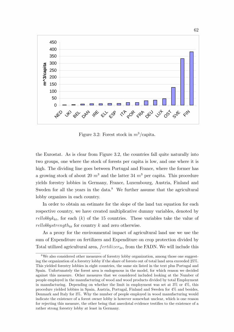
62
050
100150200250300350400450
NEDUKI
BELDAN
IRE
ELLESP ITA
PORFRA
DEULU
XOST
SVE FIN
m^3
/cap
ita
Figure 3.2: Forest stock in m3/capita.
the Eurostat. As is clear from Figure 3.2, the countries fall quite naturally into
two groups, one where the stock of forests per capita is low, and one where it is
high. The dividing line goes between Portugal and France, where the former has
a growing stock of about 20 m3 and the latter 34 m3 per capita. This procedure
yields forestry lobbies in Germany, France, Luxembourg, Austria, Finland and
Sweden for all the years in the data.8 We further assume that the agricultural
lobby organizes in each country.
In order to obtain an estimate for the slope of the land tax equation for each
respective country, we have created multiplicative dummy variables, denoted by
rellobbykkt, for each (k) of the 15 countries. These variables take the value of
rellobbystrengthkt for country k and zero otherwise.
As a proxy for the environmental impact of agricultural land use we use the
sum of Expenditure on fertilizers and Expenditure on crop protection divided by
Total utilized agricultural area, fertilizerkt, from the FADN. We will include this
8We also considered other measures of forestry lobby organization, among those one suggest-ing the organization of a forestry lobby if the share of forests out of total land area exceeded 25%.This yielded forestry lobbies in eight countries, the same six listed in the text plus Portugal andSpain. Unfortunately the forest area is endogenous in the model, for which reason we decidedagainst this measure. Other measures that we considered included looking at the Number ofpeople employed in the manufacturing of wood and wood products divided by total Employmentin manufacturing. Depending on whether the limit in employment was set at 3% or 4%, thisprocedure yielded lobbies in Spain, Austria, Portugal, Finland and Sweden for 4% and besides,Denmark and Italy for 3%. Why the number of people employed in wood manufacturing wouldindicate the existence of a forest owner lobby is however somewhat unclear, which is one reasonfor rejecting this measure, the other being that anecdotal evidence testi�es to the existence of arather strong forestry lobby at least in Germany.

63variable in levels and squared, as fertilizer2kt. Furthermore, an inspection of the
land tax/subsidy data reveals a structural break in the CAP policy. The new area
subsidies were introduced in the EU countries either from the beginning of 1993
or 1994. For this reason, for those countries that introduced the new scheme in
1993 we have included the dummy variable cap1993kt that takes a value of one
for 1990-92 and zero otherwise. For those countries that introduced the scheme
in 1994 we included the dummy variable cap1994kt, which takes the value of for
1990-93 and zero otherwise.
The construction of a variable measuring the level of technology, wheatkt, was
explained above. Alternative proxies to technology are the number of tractors
per hectare of agricultural land (tractorkt) or the number of internet users per
100 individuals in the population (internetkt). However, for tractorkt there is no
data available for Luxembourg and the Belgian �gures also include the tractors
in Luxembourg. For internetkt it is questionable how well a measure of internet
users out of the total population actually captures the level of technology in agri-
culture. In order to include the possible interaction e¤ect between technology and
lobby strength we include the interaction variable lobbywheatkt (lobbytractorktand lobbyinternetkt when tractorhakt and internetkt are included in the regres-
sion, respectively). To study the possible interaction with expenditure on fertil-
izers and crop protection, we have created the interaction variable fertwheatkt(ferttractorkt, fertinternetkt) and fert2wheatkt (fert2tractorkt, fert2internetkt).
3.3.2 Speci�cation of the Equations
Equation (3.7) constitutes the basis for the empirical speci�cation. However,
strictly taken, we cannot claim to test the theoretical model as we do not have an
alternative hypothesis against which to test the performance of the model. The
problem arises from the fact that unfortunately, we are not aware of a suitable
alternative model against which we might test our model. Nevertheless, we test
for the zero restriction on coe¢ cients, and a rejection of this null will be inter-
preted as lending support for the theoretical model. We will further compare the
performance of our model against the hypothesis presented in Bombardini [4] to
examine if the explanation forwarded by her to explain the strength of various
lobbies bears more weight than the simple model constructed here.
In order to go from the theoretical speci�cation to an empirical one, we need
to introduce an error term and specify its distribution. We assume the error term
to be iid with mean zero and variance �2 and introduce it as additive to the rest

64of the variables, so that the estimating equation becomes
landtaxkt = a10+
15Xk=1
a1krellobbykkt+a116fertilizerkt+a
117fertilizer
2kt+X
1kta
1+e1kt;
(3.12)
where X1kt is a vector of the dummy variables cap1993kt and cap1994kt indicating
changes in the CAP policy. The elasticities of land demand entering into the
calculation of rellobbykkt, agrlobbykt and forlobbykt are estimated from
agrareakt = cA0 +
15Xk=1
cAk rWACCkkt + cA16wheatkt +X
Aktc
A + eAkt (3.13a)
and
forareakt = cF0 +
15Xk=1
cFk rWACCkkt + cF16wheatkt +X
Fktc
F + eFkt: (3.13b)
Xikt is a vector of controls including wagekt, agrprodkt and forprodkt. We expect
the coe¢ cients of interest, cik, to be negative since land demand is expected to
fall as the cost of land increases. We further expect cA16 to be positive so that
technological progress in agriculture increases land demand by agriculture, and cF16to be negative so that technological progress in agriculture reduces land demand
by forestry.
Using the slope coe¢ cient estimates from equation (3.13a), the price elasticity
of land demand in agriculture in each country and each time period is calculated
as agrelastkt = �cAkrWACCkt
agrareakt. Similarly, from (3.13b) we obtain for the forestry
sector forelastkt = �cFkrWACCkt
forareakt. The thus calculated elasticities vary both among
countries and among the periods. This is assumed to depend on the changes
in the underlying variables, namely the output price of good j and changes in
technologies.
Following proposition 3.1 we expect the sign of a1k in (3.12) to be positive so
that if land demand by agriculture becomes more inelastic, re�ecting an increase in
the strength of the agricultural lobby, � 1agrelastkt
+ 1forelastkt
falls thus lowering the
land tax. If land demand by forestry becomes more inelastic, re�ecting an increase
in the strength of the forestry lobby, the term increases therefore increasing the
tax. Both the sign of a116 and of a117 are expected to be positive so that an increase
in the environmental impact of agriculture leads to an increase in the land tax
rate.
In order to examine the e¤ect of technological change on land taxation, we
also estimate the following equation, where the e¤ect of technology is given by its

65interaction with lobby strength and the use of fertilizers:
landtaxkt = a20 +
15Xk=1
a2krellobbykkt + a216fertilizerkt + a
217fertilizer
2kt
a218lobbywheatkt + a219fertwheatkt + a
220fert
2wheatkt +X1kta
1 + e1kt: (3.14)
To test the robustness of the technology variable, we further estimate equations
including the interactions of internetkt and the interactions of tractorkt instead
of the interactions of wheatkt.
The expected signs of the coe¢ cients on the added variables in (3.14) follow
from proposition 3.2. Thus, we expect the sign of a218 to be negative if the govern-
ment is susceptible to lobbying; but zero otherwise. a219 is expected to be negative,
and a220 is expected to be positive.
3.4 Empirical Results
3.4.1 Estimating the Elasticities
In estimating the elasticities of land demand in agriculture and forestry (equations
(3.13a) and (3.13b), respectively), which are used to calculate a measure of lobby
strength, the Woolridge [29] test indicated autocorrelation in the errors and the
likelihood ratio test indicated heteroscedasticity. For this reason we used feasible
GLS correcting both for heteroscedasticity and autocorrelation (AR(1) errors) in
the estimation (see, e.g., Baltagi [2], Greene [21] or Hsiao [23] for how to correct
for these ailments in error terms). The results from the regression are given in
Table 3.4 in the Appendix.
As can be seen fromTable 3.4, some of the estimates of parameters�cA1 ; :::; c
A15
and
�cF1 ; :::; c
F15
have a signi�cant positive sign, whereas others are insigni�cant.9
In order to avoid an unnecessary loss of observations, we have kept even the pos-
itive estimates, and obtain consequently negative estimates for the elasticity of
land demand for these countries. Similarly, we have used the insigni�cant values
where they exist to calculate the elasticities for those countries. The calculation
of the elasticities of land demand using the parameter estimates was explained in
Section 3.3.2.9Possible reasons for positive and signi�cant estimates include, along the lines of Shiells et
al. [28]: 1. industry characteristics and/or nonprice factors that have been omitted, or 2. themeasure of the cost of land, rWACC , may not have captured underlying price changes. It isfurther possible that there is too little variation in the land use variable, especially for forestry,for the elasticity to be estimated correctly.

66Country i Obs Mean Std. devFrance A 13 58.45 7.141
F 13 18.57 1.935Spain A 14 39.43 10.42
F 12 0 0Italy A 14 29.62 5.962
F 12 0 0The Netherlands A 14 15.32 4.651
F 14 0 0Luxembourg A 14 8.213 1.231
F 13 6.035 .9481Germany A 14 7.875 1.076
F 13 5.948 .8451Ireland A 14 5.539 1.174
F 12 0 0Denmark A 14 4.769 1.184
F 14 0 0Portugal A 14 4.302 1.479
F 13 0 0United Kingdom A 13 3.252 .5835863
F 13 0 0Belgium A 14 2.944 .2007
F 14 0 0Austria A 8 2.322 .1915
F 7 3.163 .2765Greece A 12 1.251 .1889
F 12 0 0Finland A 8 .1396 .0222
F 7 1.525 .2450Sweden A 8 .0568 .0048
F 6 .7474 .0734
Table 3.1: The strength of lobby i=A, F in each respective country, absolute valueof the lobby strength estimate.
In order to use the elasticity estimates in the land tax equation, we construct
variables for the strength of each respective lobby. We report these in Table 3.1.
The countries are listed in the decending order of the absolute mean strength of
their agricultural lobby. The table is topped by France, followed by Spain and
Italy, while the countries having the weakest agricultural lobbies are Finland and
Sweden.
3.4.2 Estimates for the Land Tax
The estimation results of the land tax equation (3.12) are given in Table 3.5,
column (2) in the Appendix; Column (1) contains a regression with fertilizer

67entered only linearly. Results for the technology variables (3.14) are given in Table
3.6. Even here we run the regressions using feasible GLS (Baltagi [2], Greene [21],
Hsiao [23]), correcting both for heteroscedasticity and for autocorrelation (AR(1)
errors). The reason is that the Woolridge [29] test indicated autocorrelation and
that the likelihood ratio test indicated heteroscedasticity of the errors, as shown
in Tables 3.5 and 3.6. Moreover, since we lack data for tractorkt for Luxembourg
in column (3) of Table 3.6, the variables rellobbyluxkt were dropped from the
regressions including this variable.
In our interpretation we will here concentrate on column (2) of Table 3.5. The
reason for including column (1) was merely to show that fertilizer, if entered
only linearly into the regression, does not get a signi�cant coe¢ cient, but that
the e¤ect from this variable is non-linear. Nevertheless, column (1) illustrates
the robustness of the coe¢ cient estimates for the rest of the variables even in the
presence of omitted variables.
The interpretation of the variable rellobbykkt in column (2) of Table 3.5 is
somewhat involved. Theoretically, if the variable rellobbykkt takes a positive value,
this indicates that the forestry lobby is stronger than the agricultural one, and vice
versa if the variable is negative. Then, if the coe¢ cient for rellobbykkt is positive,
a fall in the strength of the agricultural lobby or an increase in the strength of
the forestry lobby would lead to an increase in the land tax. Similarly, if land
demand in agriculture would become more inelastic and that sector�s lobby would
thereby become strengthened, rellobbykkt would fall and the land tax would fall
(the land subsidy would increase). Among the countries where the forestry lobby
does organize, none has a negative estimate for the elasticity of land demand in
both sectors. This poses the �rst interpretation di¢ culty. The second di¢ culty
arises from the fact that some countries where the forestry lobby does not organize
have negative elasticities of land demand in agriculture. A negative elasticity in
rellobbykkt = � 1agrelastkkt
+ 1forelastkkt
leads to that lobby�s in�uence going in the
same direction as the competing lobby�s.
Based on a comparison between the results and the signs of the elasticities
of land demand in the two sectors, we come to the following interpretation: in
essence, the agricultural lobby determines the sign of the coe¢ cient for rellobbykkteven in those countries where the forestry lobby organizes. Thus, for those coun-
tries for which the elasticity of land demand in agriculture is positive, the coe¢ -
cient for rellobbykkt is as a rule positive.10 Then, the e¤ect of lobbying works the
same way as described above: a strengthening of the agricultural lobby is man-
10Only counting those countries that have coe¢ cients signi�cant at least at the 10% level, thisapplies to Germany, (Greece), Italy, Finland and Sweden. The exception is the Netherlands,where the elasticity of land demand in agriculture is negative but the coe¢ cient on rellobbynedktis negative and signi�cant at 1%.

68ifested by the elasticity of land demand approaching zero from the right, which
leads to a fall in rellobbykkt and lowers the land tax. For those countries that have
a negative elasticity of land demand in agriculture, the coe¢ cient for rellobbykktis as a rule negative. In this case, the agricultural lobby is stronger the closer
its elasticity of land demand is to zero, but approaching from the left. Then, a
fall in rellobbykkt signi�es a strengthening of the agricultural lobby, and the land
tax falls lower the stronger the lobby is, because of the negative coe¢ cient for
rellobbykkt. Only considering those countries that have coe¢ cients signi�cant at
the 10% level, this works for Denmark and the UK. The coe¢ cients for the rest
of the countries are insigni�cant at the 10% level of signi�cance. Therefore, in
order to interpret the coe¢ cients for rellobbykkt, we need to know the sign of the
elasticity of land demand in agriculture for the country in question.
Turning to the measure of the environmental impact of agriculture on land
taxation, fertilizerit and fertilizer2 in column (2) of Table 3.5, the linear e¤ect
is negative, which is rather surprising; but the squared e¤ect is positive, as pre-
dicted. The marginal e¤ect of expenditure on fertilizers and crop production at
the minimum expenditure level (57.19 e/ha) on the land tax is �0:1345, at themean value of the expenditure (158.7 e/ha) it is �0:0208 and at the maximumexpenditure (409.8 e/ha) it is 0:2608. At low levels of expenditure on fertilizers
and crop production we thus �nd that this expenditure actually lowers the land
tax, which is contrary to the theoretical predictions. Only at a high enough level
of expenditure will the e¤ect be to raise the land tax.
The results for the technology variables included in a regression given by equa-
tion (3.14) are shown in Table 3.6; Table 3.7 gives the correlation between some of
the included variables. From column (1) of Table 3.6 it is clear that lobbywheatkt,
fertwheatkt, and fert2wheatkt are insigni�cant. Thus, either there is no e¤ect
from technology directly on the land tax, the yield of wheat per hectare is not a
good proxy for this or the insigni�cant coe¢ cient has to do with the fact that we
already used this variable to estimate the land demand elasticities explained in
section 3.4.1.
Turning to the alternative de�nitions of the level of technology, lobbyinternetki,
fertinternetkt and fert2internetkt, all are signi�cant but get signs opposite to
those predicted in proposition 3.2. However, as we already noted above, it is not
clear why the number of internet users out of 100 individuals in the population
would be a good proxy for the level of technology in agriculture.
Finally, lobbytractorki is insigni�cant but ferttractorkt and fert2tractorkt are
highly signi�cant and get the predicted signs. This yields some credence to our
hypothesis that technological change a¤ects land taxation, but combined with the
inconclusive results for the other proxies used, we take these results with some

69caution.
We end this section by examining an alternative theoretical speci�cation based
on Bombardini [4], without presenting the underlying theory in any detail. Bom-
bardini�s argument is that the size of a �rm a¤ects its incentives to participate
in industry lobbies: larger �rms are more likely to lobby. She tests her theory by
estimating an equation for the coverage ratio of non-tari¤ barriers to imports in-
cluding measures for the average �rm size in industry i and the standard deviation
of �rm size, �nding empirical support for the theory. Following her argument, in
order to ascertain ourselves that we have not missed some crucial variables from
our examination of the determination of land taxes, we run the following regres-
sion:
landtaxkt = a30 +
15Xk=1
a3krellobbykkt ++a316fertilizer + a
217fertilizer
2
+ a318firm_sizekt +X3kta
3 + e3kt; (3.15)
where we will use two di¤erent measures of firm_size, namely econsizekt, which
measures the average farm size in each respective country in European Size Units
(see European Commission [12]) and net_inckt, which gives the net income of a
farm calculated as the gross farm income minus the balance of current subsidies
and taxes in 1995 constant ECU/Euro.11
As for the sign of the new variable, Bombardini�s argument is that sectors
with larger �rms and a greater spread of �rm sizes lobby more and therefore have
a greater impact on trade protection. Translated into our model, the argument
would predict that a greater average farm size leads to greater farmer contributions
to the farmer lobby, which in turn would result in lower land taxation. The
expected sign of a318 is thus negative. The results from the regressions in (3.15)
are given in columns (3) and (4) of Table 3.5.
With regard to the coe¢ cients of the variables measuring the e¤ect of lobby
strength, rellobbykkt, the results are very similar to column (2), further empha-
sizing the robustness of the model. Also the coe¢ cients on fertilizerkt and
fertilizer2kt are signi�cant at least at the 10% level, and the squared term still gets
the predicted sign. The coe¢ cient for econsizekt is further signi�cant at the 10%
level and has the predicted negative sign. However, the coe¢ cient on net_incktis insigni�cant, although it has the predicted sign.
We thus conclude that land taxation policy in Europe seems to be partly driven
11Unfortunately we do not have data for the standard deviation of farm size in the di¤erentcountries.

70by what we interpret to be environmental concerns, but in a non-linear way so
that at a low level of impact from expenditure on fertilizers and crop protection,
the land tax actually falls in the expenditure, whereas at higher levels it increases.
Whether we have actually captured an e¤ect from environmental concerns by our
proxy or not might, however, be disputed, as it might be measuring something
else as well. What this other "thing" that fertilizerkt might be measuring is
not obvious, however, and therefore we are happy to stick to our de�nition of
concern for negative externalities. The support for Bombardini�s hypothesis is
not conclusive either, considering that one of the measures included fares fairly
well but the other one does not. Nevertheless, it seems that the size of farms might
have an impact. Finally, it is clear that the elasticity of land demand in agriculture
has a strong e¤ect on land taxation, and that this e¤ect goes in the opposite
direction from the regular public economics prediction, which stipulates that taxes
on sectors with more inelastic (land) demand should be higher. Therefore, we
deem to have found a political economy e¤ect from agricultural lobbying on land
taxation in Europe.
3.5 Conclusions
In this paper we test a theoretical model developed in Jussila Hammes [24], ex-
plaining the rarity of land taxation and the spread of land subsidies in the Euro-
pean Union, using data from 15 EU countries covering mainly the years 1990-2002.
We present a hypothesis according to which land taxation is in essence determined
by only two variables, namely the relative strength of the agricultural and forestry
lobbies as measured by their inverse elasticity of land demand to land price, and
by environmental factors. We further study whether technological change in agri-
culture can be expected to a¤ect the determination of land taxation.
The empirical �ndings give general support to the hypothesis that relative
lobby strength drives land taxation. Thus, the countries with signi�cant coe¢ -
cients for the lobby strength variable have the expected sign on that variable. The
main indication from this is that a strengthening of the agricultural lobby in a
country lowers its level of land taxation. The result seems rather robust.
We further found support for the hypothesis that expenditure on fertilizers and
crop protection positively a¤ects the land tax. Our results are, however, quali�ed
in the sense that the e¤ect is positive only at high levels of expenditure; at low
levels of expenditure it actually serves to lower the tax rate. We also found some
support for the hypothesis forwarded by Bombardini [4] that a larger average
economic size of farms should lower land taxation. The support found for this

71theory is rather tentative, however.
We also obtained some support for including technology directly into the es-
timating equation. Thus, for one of the proxies used for technology, the interac-
tion term between technology and expenditure on fertilizers and crop protection,
and the interaction with squared expenditure, were signi�cant and got the ex-
pected signs. These results are taken to broadly indicate a certain disregard by
the government of the lobbies in the face of technological progress in agriculture.
However, according to the theory, technological progress works mainly through its
e¤ect on land demand. The evidence from the regressions of land demand against
among other variables a proxy for technology is mixed, however, indicating that
agricultural technologies impact the forest area negatively, but does not show an
e¤ect on agricultural land demand directly. This aspect of the matter would thus
require further study and possibly more advanced econometric modeling.

72

Bibliography
[1] T. S. Aidt. Political internalization of economic externalities and environ-
mental policy. Journal of Public Economics, 69(1):1�16, 1998.
[2] B. H. Baltagi. Econometric Analysis of Panel Data. John Wiley and Sons,
Ltd., Chichester, second edition, 2001.
[3] E. B. Barbier and R. Damania. Corruption, trade and resource conversion.
Paper presented at the Workshop on "Trade, Biodiversity and Resources",
University of Tilburg, the Netherlands, September 5-6, 2002, July 2003.
[4] M. Bombardini. Firm Heterogeneity and Lobby Participation. PhD thesis,
Massachusetts Institute of Technology, 2004.
[5] G. A. Calvo, L. J. Kotliko¤, and C. A. Rodriguez. The incidence of a tax on
pure rent: A new (?) reason for an old answer. Journal of Political Economy,
87(4):869�874, 1979.
[6] R. Damania, P. G. Fredriksson, and J. A. List. Trade liberalization, corrup-
tion, and environmental policy formation: Theory and evidence. Journal of
Environmental Economics and Management, 46:490�512, 2003.
[7] A. Dixit. Special-interest lobbying and endogenous commodity taxation.
Eastern Economic Journal, 22(4):375�388, 1996.
[8] J. Eaton. Foreign-owned land. American Economic Review, 78(1):76�88,
1988.
[9] J. Ederington and J. Minier. Reconsidering the empirical evidence on the
Grossman-Helpman model of endogenous protection. Working Paper Series,
April 2003.
[10] T. Eicher and T. Osang. Protection for sale: An empirical investigation:
Comment. American Economic Review, 92(5):1702�1710, 2002.
[11] European Commission. Commission regulation (EC) no 1837/2001. O¢ cial
Journal of the European Communities, 2001.
73

74[12] European Commission. Community committee on the farm accountancy data
network (FADN): De�nitions of variables used in FADN standard results,
2002. RI/CC 882 Rev. 7.0.
[13] FAOSTAT Data. Last accessed October, 2004.
[14] M. Feldstein. The surprising incidence of a tax on pure rent: A new answer
to an old question. Journal of Political Economy, 85(2):349�360, 1977.
[15] P. G. Fredriksson. The political economy of pollution taxes in a small open
economy. Journal of Environmental Economics and Management, 33:44�58,
1997.
[16] P. G. Fredriksson and M. Mani. Trade integration and political turbulence:
Environmental policy consequences. Advances in Economic Analysis and
Policy, 4(2), 2004.
[17] P. G. Fredriksson and J. Svensson. Political instability, corruption and policy
formation: The case of environmental policy. Journal of Public Economics,
87:1383�1405, 2003.
[18] K. Gawande and U. Bandyopadhyay. Is protection for sale? Evidence on
the Grossman-Helpman theory of endogenous protection. The Review of
Economics and Statistics, 82(1):139�152, 2000.
[19] H. George. Framåtskridandet Och Fattigdomen : En Undersökning Af Or-
saken Till de Industriella Kriserna Och Fattigdomens Tillväxt Jemsides Med
Tillväxande Rikedom. Schultz, Upsala, 1884.
[20] P. K. Goldberg and G. Maggi. Protection for sale: An empirical investigation.
The American Economic Review, 89(5):1135�1155, December 1999.
[21] W. H. Greene. Econometric Analysis. Prentice Hall International, Inc., New
Jersey, fourth edition, 2000.
[22] G. M. Grossman and E. Helpman. Protection for sale. American Economic
Review, 84:833�850, 1994.
[23] C. Hsiao. Analysis of Panel Data. Cambridge University Press, Cambridge,
second edition, 2003.
[24] J. Jussila Hammes. Land Taxation, Lobbies and Technological Change: Inter-
nalizing Environmental Externalities. PhD thesis, University of Gothenburg,
2005.

75[25] R. W. Lindholm. Public choice and land tax fairness. American Journal of
Economics and Sociology, 38(4):349�356, 1979.
[26] D. Ricardo. On the Principles of Political Economy and Taxation. Batoche
Books, Kitchener, Ontario, Canada, 1817. Reprinted in 2001.
[27] J. Schleich. Environmental quality with endogenous domestic and trade poli-
cies. European Journal of Political Economy, 15:53�71, 1999.
[28] C. R. Shiells, R. M. Stern, and A. V. Deardor¤. Estimates of the elastici-
ties of substitution between imports and home goods for the United States.
Weltwirtschaftliches Archiv, 122(3):497�519, 1986.
[29] J. M. Wooldridge. Econometric Analysis of Cross Section and Panel Data.
MIT Press, Cambridge, MA, 2002.
[30] World Bank. World development indicators. CDROM, 2002.

763.A Appendix
Variable Explanationagrarea Agricultural area as a percentage of total land areaagrlobby Estimated strength of the agricultural lobbyagrprod Total output of (crops&crop production + livestock&livestock
products) per hectare in 1995 constant ECU/Euro per hectareeconsize Economic size of holding expressed in European size unitsfertilizer Expenditure on fertilizers and crop protection per hectare in
1995 constant ECU/Euro per hectareforarea Forestland area as a percentage of total land areaforlobby Estimated strength of the forestry lobbyforprod Roundwood production in m3 per hectaregdp_cap GDP per capita in 1995 constant ECU/EuroIF Indicator variable taking the value of one if forestry lobby in
country k organizes.internet Internet users per 100 individuals in the populationlandtax Land tax/subsidy per hectare in 1995 constant ECU/Euro per
hectarenet_inc Net income of the farm: gross farm income - balance current
subsidies & taxes in 1995 constant ECU/Eurorellobbystrength Estimated relative strength of the two lobbies: -1=agrlobby+
(IF=forlobby)rWACC Weighted average cost of capital, proxy for cost of land (and
capital)wage_h Wages and social security charges of wage earners in 1995
constant ECU/Eurowheat Yield of wheat in 100 kg per hectaretractorha Number of tractors per hectare
Table 3.2: List of variables

77Variable Obs Mean Std. Dev. Min Maxagrarea 208 .4652 .1807 .0704 .7455agrlobby 188 -3.173 21.43 -61.09 71.39agrprod 189 2324 1943 596.5 9251econsize 189 43.20 30.13 5.7 137.7fertilizer 189 158.7 80.48 57.19 409.8forarea 195 .2890 .1777 .0710 .7612forlobby 175 .6130 6.572 -22.31 21.03forprod 181 2.870 1.404 .5755 7.9gdp_cap 203 19722 7283 7900 45300internet 194 11.58 14.73 0 57.31landtax 177 -62.71 61.43 -176.6 54.12net_inc 189 35916 25721 3808 110004rellobbystrength 175 -3.153 26.35 -61.1 93.7rWACC 189 .0835 .0406 .015 .2102wage 189 5287 5341 535 23614wheat 189 57.12 21.92 0 109.1tractorha 194 62.01 25.05 26.7 108.6
Table 3.3: Summary statistics

78
Dependent vari-able:
agrareakt forareakt
rWACCbel -0.7785056*** -0.293096***(.0482315) (.0705559)
rWACCden 1.355016*** -1.571366***(.1424403) (.2172002)
rWACCdeu -0.7515357*** 0.6026201***(.1595806) (.1140492)
rWACCell -1.520815*** -0.2299352***(.1119753) (.0792161)
rWACCesp -0.1419929*** 0.0975611(.0477221) (.0705923)
rWACCfra 0.0543783** -0.0859813**(.0248438) (.042575)
rWACCire 1.888549*** -3.768449***(.2676372) (.3742937)
rWACCita -0.2429307** -0.2729497*(.108033) (.1466985)
rWACC lux -0.6176339*** 0.5861839***(.1141742) (.1055002)
rWACCned -0.3944809*** 0.0016871(.0982068) (.1815456)
rWACCost -1.414034*** 1.000711***(.0522203) (.0608267)
rWACCpor -1.263744*** 0.3881291***(.1565942) (.111149)
rWACCfin -3.054602*** 2.963305***(.5676258) (.5533346)
rWACCsve -14.24265*** 8.164517***(1.524096) (.9537566)
rWACCuki 2.812686*** -2.616738***(.4816264) (.4157366)
wheat -.0000228 -.0002399**(.0000628) (.0001169)
Observations 161 161LR test, �2 (14) 254.36 245.60Woodridge test,F (1; 14)
29.702 15.438
Table 3.4: Agricultural and forestry land demand function slope estimates. FGLSregressions. Standard errors in parentheses are adjusted for heteroscedasticity andautocorrelation (panel-speci�c AR(1) errors). ***, **, * denote signi�cance at the1, 5 and 10 percent levels, respectively. Each regression includes a constant anda number of control variables, not reported.

79
Dep. var. landtax (1) (2) (3) (4)
rellobbybel 3.758 .3565 -2.360 .8261(2.669) (2.972) (4.357) (2.850)
rellobbyden -10.63** -9.622** -7.809* -8.691*(4.163) (4.155) (4.377) (4.480)
rellobbydeu 4.941*** 4.551*** 4.324*** 4.609***(1.436) (1.447) (1.265) (1.395)
rellobbyell 22.81* 16.80 24.58* 18.47(13.13) (12.28) (13.56) (13.30)
rellobbyesp .0744 .1037 .3332 .1466(.1844) (.1772) (.2116) (.2255)
rellobbyfra -.1647 -.0731 -.3264 -.1344(.4387) (.4246) (.3467) (.4170)
rellobbyire 4.295 3.947 2.564 3.725(3.117) (3.131) (3.100) (3.212)
rellobbyita 1.126** .9165* 1.257*** 1.119***(.4852) (.4875) (.4723) (.4246)
rellobbylux .3810 .1513 .0302 .2358(.4263) (.4197) (.4774) (.4191)
rellobbyned -2.075*** -2.239*** -3.428*** -2.268***(.5842) (.5930) (1.045) (.5823)
rellobbyost 1.674 1.627 3.084 1.887(4.956) (4.998) (5.055) (5.023)
rellobbypor 1.936 3.039 4.594** 3.261(2.498) (2.541) (2.271) (2.674)
rellobbyfin 20.67*** 17.45** 19.60*** 18.76**(6.729) (7.062) (6.991) (7.549)
rellobbysve 49.70*** 50.88*** 53.33*** 52.17***(10.63) (10.16) (11.81) (11.13)
rellobbyuki -6.645*** -5.607*** -2.687 -5.829***(2.191) (2.148) (3.172) (2.185)
fertilizer .0620 -.1986* -.2222* -.1769*(.0388) (.1178) (.1312) (.1016)
fertilizer2 .00056** .00062** .00052**(.00025) (.00028) (.00021)
econsize -.3177*(.1881)
net_inc -.000029(.00015)
Observations 163 163 163 163LR test, �2 (14) 110.1 112.4 98.98 100.4Woolridge test,F (1; 14)
14.91 15.17 14.49 15.19
Table 3.5: FGLS regressions. Standard errors in parentheses are adjusted for het-eroscedasticity and autocorrelation (AR(1) errors). ***, **, * denote signi�canceat the 1, 5 and 10 percent levels, respectively. Each regression includes a constantand two dummy variables, cap1993 and cap1994, not reported.

80Dep. var. landtax (1) (2) (3)
rellobbybel .5035 .9652 5.547(3.699) (2.998) (5.079)
rellobbyden -9.217** -8.667* -7.682**(4.323) (4.451) (3.833)
rellobbydeu 4.595*** 4.836*** 5.129***(1.447) (1.512) (.9753)
rellobbyell 24.68** 16.78 31.56**(12.09) (13.74) (12.62)
rellobbyesp .0114 .2567 -1.345(.4327) (.2290) (.8770)
rellobbyfra -.0406 -.1491 .4601(.6615) (.3899) (.7926)
rellobbyire 3.621 1.983 5.585*(3.377) (3.326) (3.368)
rellobbyita .8622 .8645* -.3948(.8850) (.4993) (2.958)
rellobbylux .1283 .7014(.4280) (.4836)
rellobbyned -2.427* -2.642*** -3.252(1.314) (1.023) (2.361)
rellobbyost 1.634 3.695544 15.29***(5.034) (4.980) (5.884)
rellobbypor 2.737 4.496** .1199(2.589) (2.252) (2.546)
rellobbyfin 17.03** 21.48*** 45.96***(7.182) (7.363) (9.983)
rellobbysve 50.96*** 64.61*** 69.87***(10.17) (13.84) (13.17)
rellobbyuki -5.778** -7.649*** 4.686(2.493) (2.469) (3.359)
fertilizer -.4024** -.2746** -2.505***(.2001) (.1256) (.3818)
fertilizer2 .0016** .00057** .0087***(.0008) (.0003) (.0013)
lobbywheat .0020 lobbyinternet .0274* lobbytractor .0330(.0154) (.0167) (.0290)
fertwheat .0018 fertinternet -.0034** ferttractor .0222***(.0020) (.0015) (.0039)
fert2wheat -.00001 fert2internet .00002*** fert2tractor -.00009***(8.6e-06) (5.8e-06) (.00001)
Observations 163 162 151LR test, �2 (14) 112.9 108.3 80.99Woolridge test,F (1; 14)
20.95 15.10 18.959
Table 3.6: FGLS regressions. Standard errors in parentheses are adjusted for het-eroscedasticity and autocorrelation (AR(1) errors). ***, **, * denote signi�canceat the 1, 5 and 10 percent levels, respectively. Each regression includes a constantand two dummy variables, cap1993 and cap1994, not reported.

81
econsize fertilizer fertilizer2 fertinternet fert2internetferttractor
fertilizer 0.5832 1fertilizer2 0.5775 0.9701 1fertinternet 0.6219 0.2528 0.2455 1fert2internet0.6384 0.4164 0.4199 0.9349 1ferttractor 0.4866 0.9254 0.9249 0.2491 0.3869 1fert2tractor 0.5427 0.9286 0.9811 0.2284 0.3907 0.9538fertwheat 0.7775 0.9106 0.9155 0.3331 0.4748 0.8543fert2wheat 0.6725 0.9155 0.9714 0.2911 0.4553 0.8905lobbyinternet-0.4457 -0.2175 -0.1993 -0.7213 -0.7358 -0.1707lobbytractor 0.0021 -0.2256 -0.1978 -0.0602 -0.1534 -0.2670lobbywheat -0.1899 -0.2815 -0.2440 -0.1227 -0.2166 -0.1682net_inc 0.9191 0.7351 0.7343 0.4452 0.5379 0.6437
Table 3.7: Correlation coe¢ cients.
fert2tractor fertwheat fert2wheat lobbyinternetlobbytractor lobbywheat
fertwheat 0.8951 1fert2wheat 0.9697 0.9569 1lobbyinternet-0.1655 -0.2716 -0.2287 1lobbytractor -0.2088 -0.1942 -0.1958 0.4264 1lobbywheat -0.1838 -0.3098 -0.2653 0.4739 0.8192 1net_inc 0.7025 0.8873 0.8063 -0.3680 -0.0945 -0.2542
Table 3.8: Correlation coe¢ cients.