1

Economic Integration and the two margins of trade: An

application to the Euro-Mediterranean agreements

Sami Bensassi*

Laura Márquez-Ramos*

Inmaculada Martínez-Zarzoso**

Abstract

According to trade theory, preferential trade agreements increase international trade through a reduction in artificial trade barriers. In recently developed models with imperfect competition and heterogeneous firms, lower trade costs increase bilateral trade through an increase of the number of exporting firms (the extensive margin of trade) and a rise in the mean value of individual shipments (the intensive margin of trade). In these models, the influence of trade costs on bilateral trade results from a combination of three parameters, which affect both margins: the distance elasticity of transportation costs, the price elasticity and the degree of firm heterogeneity. In this paper, a decomposition of a structural gravity equation derived from Chaney’s (2008) model is presented. Using highly disaggregated export data for seven countries (Algeria, Egypt, Jordan, Lebanon, Morocco, Syria and Tunisia) between 1995 and 2008, we estimate the impact of the recently signed trade agreements with the EU on both trade margins and we provide empirical evidence of the validity of the theoretical predictions.

KEYWORDS: Euro-Mediterranean agreements, Trade Integration, intensive and

extensive margins.

JEL CODES: F10

* Department of Economics and Institute of International Economics, Universitat Jaume I Campus del Riu Sec, 12071 Castellón, Spain ** Department of Economics and Institute of International Economics, Universitat Jaume I Campus del Riu Sec, 12071 Castellón, Spain and Ibero-American Institute for Economic Research, University of Goettingen, Germany. Financial support from the Spanish Ministry of Education and Science (SEJ 2007-67548).) is gratefully acknowledged. Email: martinei@eco.uji.es. The authors would like to thank the participants in the Workshop in International Economics held in Goettingen for their helpful and constructive comments.

2

1. INTRODUCTION

In 1995 the European Union (EU) and fourteen countries of the Mediterranean basin

decided to commit to a deeper economic integration by signing “new generation”

integration agreements. This commitment was named the Barcelona Process. Fourteen

years later, two of the fourteen countries have already joined the EU (Malta and

Cyprus), two are candidates to join the EU (Croatia and Turkey), and a new country,

Libya, has joined the process in 2000. Table 1 shows a summary of the trade integration

process between the EU and the Euro-Mediterranean countries:

TABLE 1 – Evolution of trade integration in the Euro-Mediterranean region

Country PTA Med to EU Commitment to the Barcelona Process

Enforcement of the new Cooperation Agreement

PTA EU to Med

Algeria 1978 1995 2005 2017 Egypt 1978 1995 2004 2016 Israel - 1995 2000 2012 Jordan 1978 1995 2002 2014 Lebanon 1978 1995 2006 2018 Libya 1978 2000 no no Mauritania 1978 1995 no no Morocco 1978 1995 2000 2012 PalestinianTerritories - 1995* 1997* 2001* Syria 1978 1995 no no Tunisia 1978 1995 1998 2008

*The agreement with the Palestinian Authority is a transitory agreement which due to the political situation has not been applied.

The first cooperation agreement including a preferential trade agreement (PTA) between

the EU and the Middle East and North Africa (MENA) countries dates from the end of

the 70’s. The PTA signed was asymmetric since the EU removed the taxes charged on

the industrial products originated from the signing countries, however, the signing

3

countries maintained trade barriers in order to protect their developing industries and to

keep revenues from custom duties.

Although trade relations between Mauritania, Libya and Syria and the EU are still today

regulated by the agreements signed 30 years ago, other MENA countries have chosen to

sign new agreements. These agreements add two main innovations. Firstly, the

agreements also open the MENA markets to the EU’s products. The signing countries

have to relax all the taxes paid on the industrial products originated from the Union in a

period of twelve years, the planning for each type of product being precisely stipulated

in the agreement. Secondly, rules of origin for the signing countries have been

modified. In the precedent agreements these rules were particularly narrow (Hoekman,

1998, Francois et al., 2005) since only products made quite entirely in the signing

country or incorporating spare parts from the EU could easily enter free of duty in the

EU.

The question of the potential effect of the new series of bilateral Euro-Mediterranean

free trade agreements on trade has been particularly controversial. A number of authors

(Deardorff et al, 1996; Deardorff, 1999; Hoekman and Konan, 1999, 2005) have

underlined that the outcome of these agreements could be negative for the MENA

countries in terms of trade, growth and revenue in a short horizon. Their views are

based on the lost revenue from import duties that the MENA countries will suffer

following the agreement and from the diversion of consumption induced by the inflow

of European products.

In the positive side, it can be argued that in a word of global production networks, a

country facing less tight rules of origin could see its export capacity increased. Indeed,

the new FTAs give the MENA countries the opportunity to increase their exports to the

4

EU by deploying a Mediterranean production network. They also force industries that

were overprotected to become more productive in order to be able to compete with

European producers in their home market. Hence, these agreements should contribute to

modify the composition of trade between the two shores of the Mediterranean Sea.

This paper aims to provide empirical evidence of the effects of the current Euro-

Mediterranean agreements on trade, particularly the effect of the adoption of new rules

of origin. In order to do so, the effect of Euro-Mediterranean trade integration is

considered by analyzing the effects on both, intensive and extensive margins (Chaney,

2008). We use data on the exports of the MENA countries1

This paper is organized as follows. Section 2 presents the theoretical framework and the

empirical model. Section 3 presents data and the methodology used. Section 4 presents

the main results. Finally, the last section concludes.

to the four biggest

continental European Countries, Germany, France, Italy and Spain.

1 We have excluded from our work Israel, the Palestinian Authority, Libya and Mauritania. Israel is excluede due to the differences between this economy compared to the other MENA countries, and the Palestinian Authority, Libya and Mauritania due to lack of data.

5

2. THE EURO-MED AGREEMENTS

To understand the impact of the Euro-Med process on exports from the Mediterranean

countries to the EU, we have to focus first on the evolution over time of the signed

agreements. We differentiate between the direct effects resulting from an increase of the

EU openness to the Mediterranean products inherent to the process and the indirect

effects that could result from an increase in openness of the Mediterranean countries to

European products.

Concerning direct effects, as we have already mentioned, industrial products originating

from the Mediterranean countries were authorized to enter free of custom duties into the

European Union since 1978. Only marginal changes have occurred since then (some

provisions concerning the United Kingdom and Ireland in 1978 have for example

disappeared). It is mainly in agricultural products that the EU opens its frontiers within

the framework of the Barcelona Process. In this paper we focus instead on the effects of

changes in the rules of origin adopted as a consequence of the new agreements. The

determination of the geographic origin of the products is crucial and could hinder all

attempts of real integration. In this sense, the rules of origin (RoO) adopted with the

Barcelona process have changed in comparison to the previously existent after 1978.

According to these, if a product is wholly obtained or produced completely within one

country the product shall be deemed having origin in that country. For a product which

has been produced in more than one country the product shall be determined to have

origin in the country where the last substantial transformation took place. The EU’s

most commonly used rule is that a substantial transformation takes place when there is

change in the product tariff classification line. An alternative criterion is that the value

of the intermediate good originated from outside the FTA has to stay under a certain

percentage (often between 40 and 50%) of the value of the final good, or a particular

6

production process is used to transform the product. The main novelty introduced by

the new agreements is the so-called diagonal cumulation, which is one of the three main

types of cumulation. The other two forms are bilateral and full cumulation. Bilateral

cumulation means that two countries within the agreement can use without any limits

materials coming from each other. All PTAs allow for bilateral cumulation. Diagonal

cumulation means that materials originated from a third country also linked by an

agreement to one of the signing countries could be used without any limits by the other

signing country. If Spain has for example an FTA with Iceland and signs an FTA with

Morocco which includes the possibility of diagonal cumulation between Iceland and

Morocco, intermediate products from Iceland used as intermediates in a Moroccan good

will be consider as originating from Morocco. Finally, full cumulation allows

intermediate processing to be split in any way between the parties to the PTA provided

that when added together all inputs used are sufficient to fulfill the rule of origin

(Augier, Gasiorek and Lai-Tong, 2005; Karray 2003). Full cumulation is currently

operated by the European Economic Area (EEA) and between the Community and

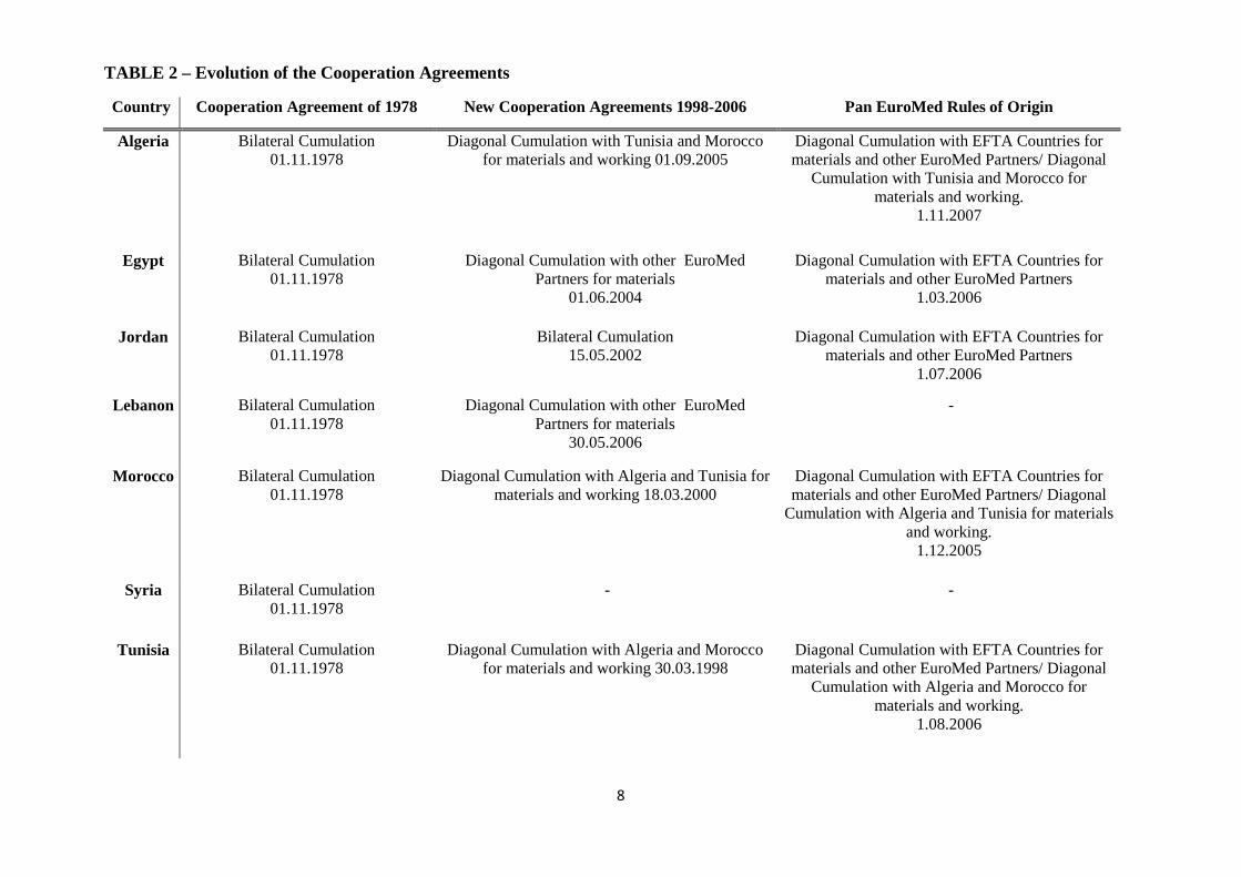
Algeria, Morocco and Tunisia. Table 2 shows how the rules concerning the cumulation

possibilities have evolved over time for the Mediterranean countries. As can be seen in

the last column of Table 2, after the adoption of the Pan-European cumulation System

in 1997 a system of Pan-Euro-Mediterranean cumulation of origin is being created. This

new system amends protocols on rules of origin annexed to the various agreements

(IP/05/1256). As noted by Augier et al. (2005) “moving to a system of diagonal

cumulation of origin widens the possible source of intermediate suppliers to all those

countries which are part of that system”. The exporters of the Mediterranean countries

could use intermediate goods from more efficient partners inside the agreement of from

7

the rest of the world2

. Consequently exports from the Mediterranean countries to EU

should increase.

2 As one of the Med countries could use intermediate goods from one of his partner in the agreement as it is its own goods it let more “space” for using intermediate goods from the rest of the world.

8

TABLE 2 – Evolution of the Cooperation Agreements

Country Cooperation Agreement of 1978 New Cooperation Agreements 1998-2006 Pan EuroMed Rules of Origin

Algeria Bilateral Cumulation 01.11.1978

Diagonal Cumulation with Tunisia and Morocco for materials and working 01.09.2005

Diagonal Cumulation with EFTA Countries for materials and other EuroMed Partners/ Diagonal

Cumulation with Tunisia and Morocco for materials and working.

1.11.2007

Egypt Bilateral Cumulation 01.11.1978

Diagonal Cumulation with other EuroMed Partners for materials

01.06.2004

Diagonal Cumulation with EFTA Countries for materials and other EuroMed Partners

1.03.2006

Jordan Bilateral Cumulation 01.11.1978

Bilateral Cumulation 15.05.2002

Diagonal Cumulation with EFTA Countries for materials and other EuroMed Partners

1.07.2006

Lebanon Bilateral Cumulation 01.11.1978

Diagonal Cumulation with other EuroMed Partners for materials

30.05.2006

-

Morocco Bilateral Cumulation 01.11.1978

Diagonal Cumulation with Algeria and Tunisia for materials and working 18.03.2000

Diagonal Cumulation with EFTA Countries for materials and other EuroMed Partners/ Diagonal

Cumulation with Algeria and Tunisia for materials and working.

1.12.2005

Syria Bilateral Cumulation 01.11.1978

- -

Tunisia Bilateral Cumulation 01.11.1978

Diagonal Cumulation with Algeria and Morocco for materials and working 30.03.1998

Diagonal Cumulation with EFTA Countries for materials and other EuroMed Partners/ Diagonal

Cumulation with Algeria and Morocco for materials and working.

1.08.2006

9

Finally, the Barcelona Process encourages the Mediterranean countries to further

integrate the service sectors (transport and finance sector for example) and to

homogenize their procedures (standardization, metrology, quality controls, and

conformity assessment) with the EU members. This measures should decreases the

transactions cost between the EU and its partners, however few progresses seems to

have been done in these domains (European Commission Reports on Neighboring 2004,

2005,2008). We will notice mainly the signature of open sky agreement between the EU

and Morocco in 2007.

In regard to the indirect effects with the Barcelona Process and the entry into force of

FTA agreements between the EU and the Mediterranean countries, the European

products will have duty free access to the south and east Mediterranean markets after a

twelve years period during which the custom duties are progressively abolished. This

change is expected to have an impact on the imports of the Mediterranean countries. As

trade barriers applied to intermediate goods from the European Union in these countries

are reduced and those intermediates became less expensive, final goods produced by

Maghreb and Mashrek exporters could also be sold at lower prices. Consequently, the

end of customs duties at the frontier of the south and east Mediterranean markets could

imply an increase in exports of these countries due to the lower costs of imported inputs.

Figure 1 shows the main expected effects of the Barcelona Process on exports from the

south and east Mediterranean countries.

10

FIGURE 1. The Barcelona Process

Note: RoW stands for Rest of the World (meaning all the countries outside the Barcelona Process)

In the empirical part of the paper we aim to estimate the overall impact of the Barcelona

Process. To do so we measure if the exports of the south and east Mediterranean

countries have increase due to the entry into force of the cooperation agreements. We

are particularly interested in the way the Barcelona Process could create trade, that is to

say we investigate if the process will impact the exports through the creation of new

trade (more varieties exported) or trough the exploitation of previously existent

comparative advantages (increase in the average quantity exported of the existing

flows). Next, we aim to specifically disentangle whether those liberalization effects are

due to a change in the rules of origin (direct effect) or to the liberalization of imported

inputs from the EU.

11

3. HETEROGENEOUS FIRMS AND THE TWO MARGINS OF TRADE

A major concern in the traditional literature on the formation of free trade agreements

(FTAs) has been whether these areas generate welfare gains for the individual countries

that engage in these processes. Since the 1950s (Viner 1950), many authors have

contributed to this debate, especially in the 1990s when studies based on the gravity

model proliferated (Frankel et al. 1995, 1996, 1998; Soloaga and Winters, 2001).

Indeed, the effect of FTAs on trade has been commonly analysed using a gravity model

of trade, with the dependent variable being the aggregate value of trade between two

countries and modelling the agreements with dummy variables. Some recent studies for

aggregated trade are Carrère (2006), Magee (2008) and Martínez-Zarzoso, Nowak-

Lehmann and Horsewood (2009). Most of these recent papers rely on a model that

assumes iceberg trade costs3

The theoretical models used to generate the gravity equation usually assume

homogeneous firms within a country and consumer love of variety. These two

assumptions imply that all products are traded to all destinations. However, empirical

observation indicates that few firms export and exporting firms commonly sell in a

limited number of countries. This empirical fact has led to the development of the so-

called new-new trade theories based on firm heterogeneity in productivity and fixed cost

of exporting (Melitz, 2003). These new theories predict the existence of a productivity

threshold for each country that firms have to exceed in order to become exporters. As a

result two margins of trade emerge: the extensive margin (the set of exporters or set of

and symmetric firms. In this setting, consumers buy

positive quantities of all varieties and aggregated trade values react to trade cost

reductions in exactly the same way as firm-level quantities and.

3 Iceberg trade costs mean that for each good that is exported a certain fraction melts away during the trip as if an iceberg were shipped across the ocean.

12

products exported) and the intensive margin (the size of its exports). Chaney (2008)

shows that a higher elasticity of substitution makes the intensive margin more sensitive

to changes in trade barriers, whereas it makes the extensive margin less sensitive. The

reasoning is as follows: when goods are highly differentiated (the elasticity of

substitution is low), the demand for each individual variety is relatively insensitive to

changes in trade costs and, then, trade barriers have little impact on the intensive margin

of trade. Otherwise, as trade barriers decrease, some firms with a low productivity level

are able to enter into the markets and, hence, when goods are highly differentiated, these

new entrants are relatively large compared to the firms that are already exporting.

Therefore, the extensive margin is strongly affected by trade barriers when the elasticity

of substitution is low. The reverse holds when the elasticity of substitution is high.

In this context we can express the quantity of a variety from origin country i to

destination country j (qij) as

( )

=

−

j

ijijij P

tpEq ~

σ

(1)

where Ej denotes country j’s total expenditure on the differentiated product, (pitij) is the

price of product i at destination j, pi varies across destinations due to positive iceberg

transport costs, tij. ( )∑ −=i

ijij tpP )1(~ σ is a price index and σ is the elasticity of

substitution, which is constant across varieties4 (CES).5

Since the quantity traded of each variety is in most cases not observable, adding two

assumptions: a) all varieties in the origin are symmetric and b) the destinations will

consume all the varieties in equal quantity, allows multiplying the quantity per variety

4 Varieties refer to different products that are substitutes in consumption. 5 The constant elasticity of substitution (CES) assumption is made in order to obtain a simple model that is easily derived and with testable implications.

13

(qij) by prices (pi) and by the number of varieties (ni) to obtain total trade values. The

outcome is

( )

==

−

j

ijiiijijiiij P

tppnEqpnT ~

σ

(2)

In equation (2) the quantity per variety is the only component of Tij that has bilateral

variation. Following Hillberry and Hummels (2008), we are able to examine each of the

components of total trade values in a more flexible way since not only data on quantities

are available, but also prices and the range of products vary across origin and

destinations. Therefore we need to relax some of the assumptions made above. Prices

may vary across destinations, if the elasticity of substitution is not constant or if

transport costs are not iceberg costs (Hummels and Skiba, 2004). Consequently for a

given year t, we can assume:

ijijijij qpnT = (3)

At least three reasons have been suggested in the literature to explain why the range of

trade products might vary with trade cost. First, goods produced in different locations

(origin and destination) can be homogeneous. In this case, if production costs in origin

and destination are very similar or the trade costs are sufficiently large, these goods will

not be traded. Additionally, the higher transport costs are, the more likely products are

to be non-traded goods. Second, if goods are differentiated by country of origin, each

country producing a different variety has to incur in a fixed cost to sell the product in

each destination country. Therefore, not all the varieties will be shipped to each

destination and the number of varieties traded will depend negatively on the magnitude

of trade costs. Finally, not all varieties are consumer goods. Intermediate inputs that are

used in the production of final goods would only be exported to destination j if country j

14

produces the final good. Due to “just in time” production processes intermediates are

more likely to be traded over short distances. We focus on the first and second

explanations and assume that both, the number of varieties and the quantity traded are

negatively affected by trade costs.

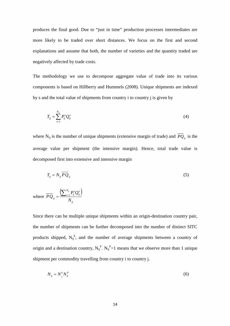
The methodology we use to decompose aggregate value of trade into its various

components is based on Hillberry and Hummels (2008). Unique shipments are indexed

by s and the total value of shipments from country i to country j is given by

∑=

=ijN

s

sij

sijij QPT

1

(4)

where Nij is the number of unique shipments (extensive margin of trade) and ijPQ is the

average value per shipment (the intensive margin). Hence, total trade value is

decomposed first into extensive and intensive margin

ijijij QPNT = (5)

where ( )

ij

sij

N

ss

ijij N

QPQP

ij∑ == 1

Since there can be multiple unique shipments within an origin-destination country pair,

the number of shipments can be further decomposed into the number of distinct SITC

products shipped, Nijk, and the number of average shipments between a country of

origin and a destination country, NijF. Nij

F>1 means that we observe more than 1 unique

shipment per commodity travelling from country i to country j.

Fij

kij NNN

ij= (6)

15

The average value per shipment can also be further decomposed into average price and

average quantity per shipment:

( ) ( )ijij

ij

N

s ijN

s ij

N

ssij

sij

ij QPN

Q

Q

QPQP

ij

ij

ij

== ∑∑∑ =

=

= 1

1

1 (7)

By substituting equations (6) and (7) into (5) we can decompose total trade between two

countries into four different components:

ijijFij

kij QPNNT

ij= (8)

The quantity measure is tons for all commodities. Using a common unit allows us to

aggregate over different products and compare prices (import unit values) across all

commodities.

We now have two decomposition levels. The first is given by equation (5) and

decomposes total trade value into the range of products traded and the average value per

product. The second, given by equation (8), decomposes these two components into

another two each: the number of distinct SITC goods shipped, the number of average

shipments between a country of origin and a destination country, and average price and

average quantity, respectively. Taking logs for the first and second level decompositions

and adding the time dimension, t we obtain:

ijtijtijt QPNT lnlnln += (9)

ijtijtFijt

kijt QPNNT

ijtlnlnlnlnln +++= (10)

Next we analyse how each of the components of equation (10) co-vary with distance

and with other trade-related costs. The variable of interest is trade cost reductions

induced by trade liberalisation between the European Union and the Maghreb countries

16

considered. Before specifying the empirical model, we state a number of hypotheses

that are based on recent theories of international trade under imperfect competition and

heterogeneous firms. Melitz (2003) introduced firm heterogeneity in a general

equilibrium model of international trade. Chaney (2008) extended Melitz’s model to

multiple countries with asymmetric trade barriers and derives three predictions for

aggregated trade. The first prediction states that for aggregated bilateral trade flows his

model predicts that the elasticity of exports with respect to trade barriers is larger than

in the absence of firm heterogeneity and larger than the elasticity for each individual

firm. A reduction of variable cost has two effects. First, it increases the size of exports

of each exporter and second, it allows new firms to enter the market. Therefore, the

extensive margin amplifies the impact of variable costs.

In more homogeneous sectors, aggregated exports are very sensitive to changes in

transportation costs because many firms enter and exit when variable costs change. The

elasticity of exports with respect to variable costs does not depend on the elasticity of

substitution between goods. However, the elasticity of exports with respect to fixed

costs is negatively related to the elasticity of substitution. This is in contrast with

models with a representative firm, according to which the elasticity of exports with

respect to transport costs equals the elasticity of substitution minus one.

Further, with respect to the two margins of trade, Chaney (2008) shows that in the

presence of firm heterogeneity, the extensive margin and the intensive margin are

affected in different directions by the elasticity of substitution. The impact of trade

barriers is strong in the intensive margin for high elasticities of substitution

(homogeneous products), whereas the impact is mild on the extensive margin. The

author proves that the dampening effect on the extensive margin dominates the

magnifying effect on the intensive margin.

17

We are interested in knowing whether these predictions hold for trade flows in the

Mediterranean region. In order to test some of the abovementioned predictions, the

estimating equation takes the following form:

ijkttkijt

ijjtitjtitjiijkt

ColonyCA

DPOPPOPGPDGDPX

ελγαα

αααααβα

+++++

++++++=

76

54321 lnlnlnlnlnln

(11)

where γk and λt are industry (at two digit level) and year fixed effects and αi and βj are

importer and exporter fixed effects. εijkt is an error term and ln(Xijkt) is in turn the log of

the average value per shipment (intensive margin), and the log of the range of shipments

(extensive margin), as described in equation (9). GDPit and GDPjt denote Gross

Domestic Product of the importer and the exporter country in year t, respectively and

POPij and POPjt denote the respective populations. Dij is the geographical distance

between the trading-countries’ capitals and FTAijt denote Free Trade Agreements

dummies that take the value of one when both countries have implemented a

cooperation agreement in year t, zero otherwise. As an extension, the change in the

agreements over the rules of origin, the quantity of intermediate products originating

from the European Union and from the Rest of the World could be included instead of

the FTA dummies to account for the transmission channels of the free trade agreements.

Finally, colony is a dummy that takes the value of one when the trading partner had a

colonial relationship in the past, zero otherwise.

Since OLS is linear, the coefficient on total imports will be equal to the sum of the

coefficients on the two margins. A further decomposition can be done, using each of the

components in equation (10) as dependent variable in equation (11).

18

4. DATA, SOURCES AND VARIABLES

The main data source is Eurostat. We use the external trade detailed database which

covers both extra- and intra-EU trade. In particular, extra-EU trade statistics provide

data for the trade in goods between the MENA countries and four Member States

(France, Italy, Germany and Spain). The products are classified according to the

Standard International Trade Classification (SITC) codes at the SITC 5-digit level. Only

manufactured products are taken into consideration (categories 5 to 8). Income and

population data are taken from the World Development Indicators Database 2008 and

distance and colonial links from CEPII. Table 3 provides a summary of the data and

sources used in this paper.

TABLE 3 – Variable descriptions and sources of data.

Dependent Variables Description Source Xij : Exports from i to j Nominal X Eurostat

Nij : Extensive Margin Number of type of products exported from i t j Eurostat

AVij : Intensive Margin Average Value of the products exported from i to j Eurostat

AQij : Average Quantity Average Quantity of the products exported from i to j Eurostat

APij : Average Price Average Price of the products exported from i to j Eurostat

19

Independent Variables Description Source Yi : Exporter’s income Exporter’s GDP, PPP (current $) WDI Yj : Importer’s income Importer’s GDP, PPP (current $) WDI

FTA dummy Dummy variable = 1 if the

trading partners have an FTA, 0 otherwise

European Commission

D_cumulation Dummy variable = 1 if the RoO allow diagonal cumulation with

the other MENA countries European Commission

Pan_EuroMed_RoO Dummy variable = 1 if the countries have adopted Pan

EuroMed RoO European Commission

Input_EUi

Import value of machinery from four European Economies

(current $) OECD

Input_RoWi Import value of machinery from the Rest of the World (current $) OECD

Distij : Distance Distances between country capitals of trading partners (km) CEPII

Colonyij : Dummy variable = 1 if the

trading partners had colonial links in the past, 0 otherwise

CEPII

The extensive and intensive margin, average price and average quantity of products

exported from the MENA to France, Italy, Germany and Spain over the period 1995-

2007 are calculated by using export values and export quantities. Among our

independent variables Input_EU and Input_RoW are used as proxies for intermediate

inputs coming from the main countries of the European Union (France, Germany, Italy,

Spain and the United Kingdom) or alternatively, from the main producers of the Rest of

the World (Japan, South Korea, Honk Kong, USA). The source for these tow variables

is the OECD database on exports and in particular we use exports from the main

20

countries of the European Union and the Rest of the world to each Mediterranean

country of Nuclear Reactors, Boilers, machinery (Section 84 of the harmonized system

commodity classification).

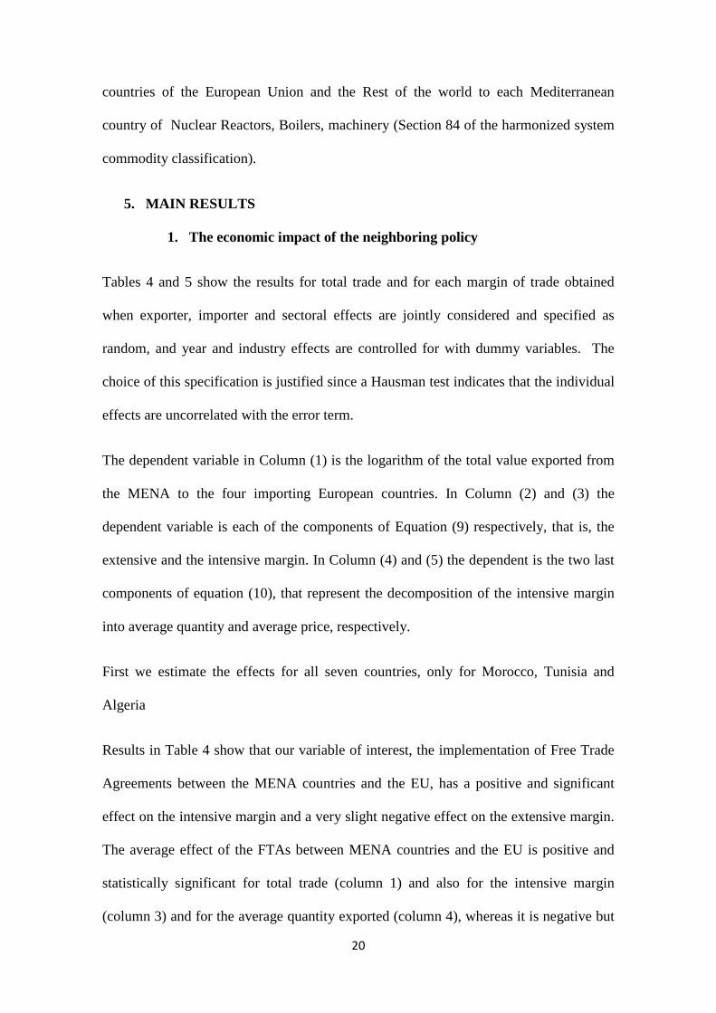
5. MAIN RESULTS

1. The economic impact of the neighboring policy

Tables 4 and 5 show the results for total trade and for each margin of trade obtained

when exporter, importer and sectoral effects are jointly considered and specified as

random, and year and industry effects are controlled for with dummy variables. The

choice of this specification is justified since a Hausman test indicates that the individual

effects are uncorrelated with the error term.

The dependent variable in Column (1) is the logarithm of the total value exported from

the MENA to the four importing European countries. In Column (2) and (3) the

dependent variable is each of the components of Equation (9) respectively, that is, the

extensive and the intensive margin. In Column (4) and (5) the dependent is the two last

components of equation (10), that represent the decomposition of the intensive margin

into average quantity and average price, respectively.

First we estimate the effects for all seven countries, only for Morocco, Tunisia and

Algeria

Results in Table 4 show that our variable of interest, the implementation of Free Trade

Agreements between the MENA countries and the EU, has a positive and significant

effect on the intensive margin and a very slight negative effect on the extensive margin.

The average effect of the FTAs between MENA countries and the EU is positive and

statistically significant for total trade (column 1) and also for the intensive margin

(column 3) and for the average quantity exported (column 4), whereas it is negative but

21

only significant at 10 percent level for the extensive margin. Turning to the second

level decomposition of equation (10), the first component of average value per shipment

(columns 4 - Table 4), average quantities shipped are higher after the FTA entered into

force, whereas the FTA variable is not significant when the average price component is

used as dependent variable.

With respect to the additional explanatory variables, we obtained the expected positive

and statistically significant effect for the GDP of the importing and exporting countries.

Geographical distance presents a negative and significant coefficient, except for the

average price, which shows a positive distance coefficient (this result has also been

obtained in results for a sample of Latin American countries, see Martínez-Zarzoso and

Wilmsmeier, 2009; Hillberry and Hummels, 2008). The decomposition of the influence

of distance on trade shows a greater effect on the intensive margin (column 3 - Table 4),

for all industrial products. About 29% of the distance effect on trade works through the

extensive margin (i.e. 0.427/(1.044+0.427)); 71% of the increase in disaggregate trade

flows comes from larger average shipments. Previous research finds the opposite

picture, with the extensive margin being more important than the intensive margin

(Hillberry and Hummels, 2008; Mayer and Ottaviano, 2008). Our results are very

different to Mayer and Ottaviano (2008), who analyze French and Belgian individual

export flows and show that 75% of the distance effect on trade comes from the

extensive margin.

Finally, sharing colonial links and language fosters exports from MENA countries to the

EU; 43% of the increase in disaggregate trade flows comes from the extensive margin (a

wider variety of products traded), whereas 57% of the increase in disaggregate trade

flows comes from larger average shipments.

22

TABLE 4 - Main estimation results for all countries and sectors

Xij Nij AVij AQij APij lgdpi_euro 1.264*** 0.287*** 0.779*** 0.658*** 0.241** 8.278 5.812 5.985 4.047 2.27 lgdpe_euro 0.290*** 0.084*** 0.228** * 0.114 -0.002 3.398 2.763 3.234 1.207 -0.028 Ld -1.507*** -0.427*** -1.044*** -1.491*** 0.414*** -9.85 -6.978 -8.765 -8.811 4.005 FTA 0.081* -0.025* 0.113*** 0.08* -0.015 1.819 -1.744 2.854 1.649 -0.451 Colony 1.273*** 0.568*** 0.743*** 0.564** 0.085 7.018 7.392 5.418 2.793 0.651 Constant -19.087*** -5.489*** -8.936** -5.81 -3.26 -4.106 -3.498 -2.296 -1.188 -1.023 R-squared 0.092 0.081 0.06 0.041 0.003 r2_o 0.1274876 0.0970905 0.094264 0.0609608 0.0298642 N 11480 11496 11480 10917 10917 Rmse 1.320634 0.4120877 1.191463 1.392733 0.9288741

Notes: ***, **, *, indicate significance at 1%, 5% and 10%, respectively. T-statistics are in brackets. The dependent variable is the natural logarithm of exports in value (current US$). Income (Y) and distance (Dist) are also in natural logarithms. The estimation uses White’s heteroscedasticity-consistent standard errors. Tval denotes total trade, Extm denotes extensive margin, Intm denotes intensive margin, Avq denotes average quantity and avp denotes average price.

Our first results consistently show that the new FTA agreements signed between the

MENA countries and the European Union have fostered export of these countries to

some of their main European partners. Furthermore, we find that this increase in exports

has been channeled by an increase of the intensive margin of trade. The MENA

countries export more of the products they already exported in the past. This fact is in

line with what we know of the industrial structure of these countries and with the

explanation proposed by Chaney (2008) concerning how reductions in trade costs

influence the two margins of trade. MENA are mainly producers of goods with low

technological content, which are highly substitutable on the international market. In this

23

case, Chaney (2008) states that the main impact of a decrease in trade barriers will be

through the intensive margin.

Next, we estimate the effects only for Maghreb countries: Morocco, Tunisia and

Algeria. The main reason is that these countries have full cumulation.

TABLE 5 - Main results for Maghreb. All Sectors

Xij Nij AVij AQij APij lgdpi_euro 1.886*** 0.426*** 1.376*** 1.265*** 0.259 7.599 5.805 6.246 5.004 1.643 lgdpe_euro -1.802*** -0.551*** -1.177*** -1.086*** -0.084 -9.796 -9.191 -7.417 -5.122 -0.659 ld -1.934*** -0.345** -1.539*** -2.016*** 0.440* -6.612 -3.05 -6.333 -5.997 2.145 FTA 0.256*** 0.032 0.213*** 0.218** -0.034 3.646 1.444 3.38 2.789 -0.675 Colony 2.089*** 0.815*** 1.282*** 1.026*** 0.148 8.57 8.045 6.57 3.637 0.816 _cons 16.500* 5.262* 11.46 9.684 -2.075 2.137 2.194 1.683 1.18 -0.405 R-squared 0.134 0.104 0.093 0.06 0.005 r2_o 0.158 0.152 0.099 0.052 0.0436 N 5207 5211 5207 5065 5065 Rmse 1.251025 0.3794191 1.143219 1.313111 0.8562009

Notes: ***, **, *, indicate significance at 1%, 5% and 10%, respectively. T-statistics are in brackets. The dependent variable is the natural logarithm of exports in value (current US$). Income (Y) and distance (Dist) are also in natural logarithms. The estimation uses White’s heteroscedasticity-consistent standard errors. Tval denotes total trade, Extm denotes extensive margin, Intm denotes intensive margin, Avq denotes average quantity and avp denotes average price.

These results show that our variable of interest, the creation of a FTA between North

African countries and the EU, has a greater effect on the intensive margin than on the

extensive margin. The effect of the FTA between North African countries and the EU is

positive and statistically significant for total trade (column 1) and also for the intensive

margin (column 3) and for the average quantity exported (column 4), whereas it is also

positive but only significant at 10 percent level for the intensive margin. The

decomposition of the influence of FTA on trade shows that this effect on trade works

24

through both margins: around 13 % works through the extensive margin and around

87% works through the intensive margin, although the estimated coefficient for the

extensive margin is only marginally significant. Turning to the second level

decomposition of equation (10) (columns 4 - Table 5), average quantities shipped are

higher after the FTA entered into force, whereas the FTA variable is not significant

when the average price component is used as dependent variable.

With respect to the additional explanatory variables, we obtained the expected positive

and statistically significant effect for the GDP of the importing country, but not for the

exporter GDP which is negatively signed and thus indicates that a higher GDP is

associated with a decrease in exports to the four European countries considered. We still

need to find an explanation for this negative effect. We also estimated the model

including population variables (or GDP per capita), but since they are highly correlated

with GDPs the coefficients cannot be jointly estimated in a consistent way.

Geographical distance presents a negative and significant coefficient, as with all the

exporting countries. The decomposition of the influence of distance on trade shows also

a greater effect on the intensive margin (column 3 - Table 5), for all sampled products.

About 18% of the distance effect on trade works through the extensive margin (i.e.

0.345/(1.539+0.345)); 82% of the increase in disaggregate trade flows comes from

larger average shipments. And finally, the variables sharing colonial links and language

present very similar results for this narrower sample of countries; 39% of the increase in

disaggregate trade flows comes from the extensive margin (a wider variety of products

traded), whereas 61% of the increase in disaggregate trade flows comes from larger

average shipments.

25

The effect of the bilateral FTAs on trade is also estimated for each sector (at one digit-

level SITC) and for each exporter. Table 6 shows the main results for the FTA variable

for each section of the SITC. The various sectors are not equally impacted by the

agreements. The coefficient of the FTA variable is non-significant for the Section 8

(Miscellaneous manufactured articles), whereas it is significant and positive for the

intensive margin and the average quantity exported for Section 5 (Chemicals and related

products), 6 (Manufactured goods classified chiefly by material) and 7 (Machinery

transport equipment). Only for Section 5 the coefficient is significant for the extensive

margin. The results are in line with the idea that the main changes induce by the FTA

come through the intensive margin of trade. In contrast, the results for each country in

Table 7 give a different picture.

TABLE 6 - Main results for each product category. Seven Countries

Xij Nij AVij AQij APij Sector

5 - Chemicals and related products

0.305*** 0.088*** 0.248** 0.243* -0.076

2.836 2.719 2.513 2.002 -1.001

6 - Manufactured goods classified chiefly by material

0.12 -0.023 0.162** 0.183* 0.038

1.387 -0.813 2.157 1.899 0.711

7 - Machinery and transport equipment

0.160* 0 0.182** 0.210** -0.056

1.974 -0.013 2.5 2.504 -0.896

8 - Miscellaneous manufactured articles

-0.043 -0.021 0.019 0.034 0.031

-0.564 -0.803 0.286 0.426 0.526 Notes: ***, **, *, indicate significance at 1%, 5% and 10%, respectively. T-statistics are in brackets. The dependent variable is the natural logarithm of exports in value (current US$). Income, population and distance are also in natural logarithms. The estimation uses White’s heteroscedasticity-consistent standard errors. Tval denotes total trade, extm denotes extensive margin, intm denotes intensive margin, vaq denotes average quantity and avp denotes average price.

The coefficient of the FTA variable is positive and significant for total exports for each

country with the only exception of Jordan for which the coefficient is positive but not

26

significant. It seems that we could divide the MENA countries into two groups: the

countries with a significant and positive coefficient for the extensive margin and a non-

significant coefficient for the intensive margin (Jordan, Lebanon and Morocco) and the

countries with a significant and positive coefficient on the intensive margin of trade and

a non-significant coefficient on the extensive margin (Algeria) or with a significant but

less important effect on the extensive than on the intensive margin of trade (Egypt and

Tunisia).

TABLE 7 - Main results for each country

Xij Nij AVij AQij APij Countries Algeria 0.942*** 0.103 0.797** 0.473 0.311 2.91 0.891 2.118 1.434 1.425

Egypt 0.739*** 0.102* 0.638*** 0.540* -0.382***

3.949 1.903 3.769 2.061 -3.648

Jordan 0.453 0.309*** 0.249 -1.084*** 0.174

1.438 2.721 0.894 -3.014 0.726 Lebanon 0.612* 0.311*** 0.251 -0.534 0.413* 2.014 3.099 0.982 -1.487 2.105 Morocco 0.484** 0.190*** 0.24 0.633*** -0.031 2.469 3.641 1.314 3.309 -0.276 Tunisia 1.272*** 0.255*** 0.619*** 0.404** 0.111 6.625 5.165 3.599 2.3 1.116

Notes: ***, **, *, indicate significance at 1%, 5% and 10%, respectively. T-statistics are in brackets. The dependent variable is the natural logarithm of exports in value (current US$). Income, population and distance are also in natural logarithms. The estimation uses White’s heteroscedasticity-consistent standard errors. Tval denotes total trade, extm denotes extensive margin, intm denotes intensive margin, vaq denotes average quantity and avp denotes average price

2. Disentangling FTA effects

We replace our variable FTA by four different variables designed to take in account

particular aspects of the agreement.

The extended model is given by

27

(12)

where D_Cumulation takes the value of one when the rules of origin allow diagonal

cumulation with the other MENA countries, zero otherwise; Pan-EuroMed_RoO takes

the value of one when a country has Pan EuroMed RoO, zero otherwise; MIEUit denotes

importer machinery from the EU and MIRoWit denotes importer machinery from the

rest of the world. Next, we estimate an extended model for all countries and for each

sector. We are not able to estimate the extended model for each country since our

variables imported inputs from the EU and from RoW are country specific.

The coefficients for Diagonal cumulation are significant and positive for total trade, the

average value of exports and their average quantity. It is negative and significant for the

average price. The coefficients for the Pan Euro Med rules of origin are significant and

positive for total trade and for the extensive margin (number of goods exported). The

coefficient of the variable Inputs from the EU is positive and significant for the average

price of the MENA exports and negative and significant for the average quantity of the

MENA exports. The coefficient of Inputs from the rest of the world is negative for total

trade and also for the number of goods exported.

TABLE 8 –Channels through which trade is impacted

Xij Nij AVij AQij APij lgdpi_euro 1.243*** 0.287*** 0.768*** 0.662*** 0.233** 8.188 5.842 5.913 4.069 2.197 lgdpe_euro 0.349*** 0.125*** 0.227** 0.355*** -0.185** 3.299 3.462 2.496 3.034 -2.396 Ld -1.367*** -0.354*** -0.982*** -1.495*** 0.473*** -8.393 -5.599 -7.527 -8.229 4.24 D_cumulation 0.125** 0.008 0.120** 0.208*** -0.112*** 2.629 0.522 2.802 3.986 -3.195 Pan_EuroMed_RoO 0.103* 0.075*** 0.027 0.065 -0.052

ijktijkijkt

ijkttkitit

ijtijjtitijkt

whereMIRoWMIEUColony

CumulationPanECumulationDDGPDGDPX

νµε

ελγααα

αααααα

+=

++++++

++++++=

876

52514210 __lnlnlnln

28

1.633 3.731 0.483 0.917 -1.11 linput_eu 0.098 0.044 0.063 -0.244** 0.250*** 1.016 1.415 0.739 -2.296 3.54 linput_row -0.177** -0.106*** -0.067 -0.064 -0.027 -2.801 -5.138 -1.208 -0.919 -0.564 Colony 1.213*** 0.534*** 0.717*** 0.537** 0.077 6.676 7.016 5.153 2.633 0.584

_cons -19.635*** -5.951*** -9.111* -5.496 -3.697

-4.232 -3.81 -2.336 -1.12 -1.156 R-squared 0.092 0.082 0.06 0.043 0.005 r2_o 0.1329493 0.1076868 0.0961964 0.0603867 0.0313113 N 11480 11496 11480 10917 10917 Rmse 1.322085 0.4123629 1.192141 1.392123 0.9279655

Notes: ***, **, *, indicate significance at 1%, 5% and 10%, respectively. T-statistics are in brackets. The dependent variable is the natural logarithm of exports in value (current US$). Income (Y) and distance (Dist) are also in natural logarithms. The estimation uses White’s heteroscedasticity-consistent standard errors. Tval denotes total trade, Extm denotes extensive margin, Intm denotes intensive margin, Avq denotes average quantity and avp denotes average price.

Interestingly, each sector of production present different impacts for each channel

(Table 9). For example, the coefficients for Diagonal Cumulation are highly significant

and positive for total trade and for the average value and the average quantity of exports

for the Section 5 and 6, whereas the coefficients for the Pan Euro Med RoO are mainly

significant and positive for total trade and for the extensive margin for section 7 and 8.

Coefficients are also significant for the input from the European Union for the same

section. The coefficients for the inputs from the RoW are significant and negative

mainly for section 8.

These results indicate that the adoption of diagonal cumulation between the MENA

countries has an impact on their export to Europe mainly through the intensive margin

of trade, and more specifically through the average quantity exported. Strikingly

different are the results to cumulate origin with new countries from the north of Europe

(Pan Euro Med RoO), for which the main effect on exports comes through the extensive

margin. The decreasing price of European input has an interesting effect, for the

29

sections with lower technological content (sections 5 and 6). The inclusion of European

inputs decreases the average quantity of the exports but increase their average price.

One could easily imagine that these results could translate an increase of the quality of

the goods produced by the MENA due to the integration of more European spare parts.

In the sector with the higher technological content, section 7, European inputs have a

strong and positive effect on both margins of trade. It is more difficult to interpret the

results for the inputs from the rest of the world.

30

TABLE 9 –Channels through which trade is impacted. Sectoral results

Xij Nij AVij AQij APij Sector

5 - Chemicals and related products

D_cumulation 0.334*** 0.092** 0.262** 0.398*** -0.156** 2.974 2.617 2.544 3.188 -1.995

Pan_EuroMed_RoO -0.165 0.117** -0.275* -0.351** 0.093 -1.14 2.403 -2.039 -2.139 0.975

linput_eu -0.166 0.009 -0.169 -0.607** 0.407** -0.706 0.127 -0.807 -2.295 2.763

linput_row -0.054 -0.022 -0.005 0.008 -0.133 -0.386 -0.513 -0.037 0.048 -1.574

6 - Manufactured goods classified chiefly by material

D_cumulation 0.334*** 0.062* 0.289*** 0.342*** -0.05 3.57 2.069 3.582 3.318 -0.857

Pan_EuroMed_RoO 0.096 0.07* 0.035 0.127 -0.064 0.75 1.709 0.311 0.869 -0.769

linput_eu -0.23 0.116* -0.325* -0.596** 0.301** -1.205 1.874 -1.932 -2.757 2.595

linput_row -0.196 -0.188*** -0.009 0.102 -0.150** -1.565 -4.615 -0.081 0.782 -2.444

7 - Machinery and transport equipment

D_cumulation 0.061 0.015 0.06 0.246** -0.194** 0.688 0.559 0.749 2.675 -2.883

Pan_EuroMed_RoO 0.217* 0.101** 0.125 0.263* -0.142 1.796 2.832 1.151 1.959 -1.456

linput_eu 0.528*** 0.149** 0.446*** 0.103 0.381** 3.175 2.748 3.01 0.593 2.901

linput_row -0.161 -0.102*** -0.081 -0.09 -0.011 -1.509 -3.026 -0.874 -0.873 -0.141

8 - Miscellaneous manufactured articles

D_cumulation 0.006 0.024 0.026 0.142* -0.051 0.071 0.873 0.361 1.657 -0.799

Pan_EuroMed_RoO 0.288** 0.082** 0.230** 0.215* 0.039 2.767 2.325 2.532 1.913 0.44

linput_eu 0.497*** 0.035 0.525*** 0.615*** -0.097 2.937 0.558 3.624 3.624 -0.775

linput_row -0.415*** -0.181*** -0.284** -0.398*** 0.051 -3.857 -4.973 -3.147 -3.581 0.692

Notes: ***, **, *, indicate significance at 1%, 5% and 10%, respectively. T-statistics are in brackets. The dependent variable is the natural logarithm of exports in value (current US$). Income (Y) and distance

31

(Dist) are also in natural logarithms. The estimation uses White’s heteroscedasticity-consistent standard errors. Tval denotes total trade, Extm denotes extensive margin, Intm denotes intensive margin, Avq denotes average quantity and avp denotes average price.

6. CONCLUSIONS

In this paper, the effect of Euro-Mediterranean agreements on international trade is

evaluated by using disaggregated trade data. These agreements should contribute to

modified trade patterns between the two shores of the Mediterranean Sea. We apply

some of recently developed models of trade (Chaney, 2008) to depict the impact of FTA

on the extensive and intensive margins of trade. We focus on exports from MENA

countries to the four biggest continental European economies, Germany, France, Italy

and Spain.

Our first results seem to confirm a positive and significant effect of the new FTA on the

exports of MENA countries to their main European partners. This effect should find its

root in the new rules of origin agreed between the two groups of countries. As we have

seen the main channel in the transformation of the structure of exports from Algeria,

Morocco, and Tunisia to their European counterparts is through the intensive margin.

More of the products already exported previously by the Maghreb countries are sent to

Europe.

A plausible explanation of the reason why the adoption of new rules of origin have

resulted in the increase of trade is that the new rules have allowed the integration of

better quality/less expensive intermediate goods in the goods produced by the Maghreb

countries consequently enhancing the demand for these goods on the European markets.

With our sectoral result we partially confirm this hypothesis, since the effect of an

increase in the inputs imported from the EU has a positive effect on MENA’s exports of

sophisticated manufactured products, with the only exception of chemicals and related

32

products. This effect is channeled by an increase of the extensive and intensive margins

of trade for machinery and transport equipment, by an increase of the extensive margin

for manufactured goods classified chiefly by material and by an increase of the intensive

margin for miscellaneous manufactured articles. Further research on more disaggregated

products is desirable to know whether export diversification is actually a consequence of the

change in the rules of origin.

33

REFERENCES

• Augier, P., Gasiorek, M and Lai Tong, C. (2005),. "The impact of rules of origin

on trade flows" Economic Policy 20(43), 567-624.

• Carrère, C. (2006), “Revisiting the effects of regional trade agreements on trade

flows with proper specification of the gravity model” European Economic

Review 50 (2), 223-247.

• Chaney, T. (2008), Distorted Gravity: The Intensive and Extensive Margins of

International Trade, American Economic Review 98:4, 1707-1721.

• Deardorff, A. (1999). Economic implications of Europe-Maghreb trade agreements.

Technical report.

• Deardorff, A., D. Brown, and R. Stern (1996). Some economic effects of the free trade

agreement between Tunisia and the European Union. Technical report.

• Francois, J. F., M. McQueen, and G. Wignaraja (2005). “European union-developing

country FTAs: overview and analysis”. World Development 33(10), 1545 – 1565.

• Frankel JA, Stein E, Wei S-J (1995) “Trading blocs and the Americas: the natural, the

unnatural, and the super-natural”. J Dev Econ 47(1):61–95

• Frankel JA, Stein E, Wei S-J (1996) Regional trading arrangements: natural or

supernatural. Am Econ Rev 86(2):52–56

• Frankel JA, Stein E, Wei S-J (1998) “Continental trading blocs: are they natural or

supernatural”. In: Frankel, JA (ed) The regionalization of the world economy.

University of Chicago Press, Chicago, pp 91–113

• Karray, B. (2003). "The Rules of Origin in the Euro-Mediterranean economic

space". In Euro-Med Integration and the 'Ring of Friends': The Mediterranean's

European Challenge, Vol IV, Xuereb, Peter G., Eds. European Documentation

and Research Centre.

34

• Hillberry, R. and Hummels, D. (2008), Trade Responses to Geographical

Frictions: A Decomposition Using Micro-Data, European Economic Review 52,

527–550.

• Hoekman, B. (1998). Free trade agreements in the Mediterranean : a regional path

towards liberalisation. The Journal of North African Studies 3(2), 89 – 104.

• Hoekman, B. and D. E. Konan (1999, May). Deep integration, nondiscrimination, and

Euro-Mediterranean free trade. Policy Research Working Paper Series 2130, The World

Bank.

• Hoekman, B. and D. E. Konan (2005). Deepening Egypt-US trade integration:

Economic implications of alternative options. Technical report.

• Hummels, D. and Skiba, A. (2004) Shipping the Good Apples Out? An

Empirical Confirmation of the Alchian-Allen Conjecture, Journal of Political

Economy, 112(6), 1384-1402.

• Magee, C.S.P. (2008), .New Measures of Trade Creation and Trade Diversion,. Journal

of International Economics, 75, 349-362.

• Martinez-Zarzoso, I. (2009), On Transport Costs and Sectoral Trade: Further Evidence

for Latin-American Imports from the European Union, forthcoming in Grabriele Tondl

(ed.) European Community Studies Association of Austria Publication Series.

• Martinez and Wilmsmeier (2010) Martinez-Zarzoso, I. and Wilmsmeier, G.

"Determinants of maritime transport costs - a panel data analysis"

Transportation Planning and Technology 33.1: 117-136.

• Martínez-Zarzoso, I., Nowak-Lehmann D., F. and Horsewood, N.. (2009) “Are

Regional Trading Agreements Beneficial? Static and Dynamic Panel Gravity

Models” North American Journal of Economics and Finance 20, 46-65.

35

• Mayer, T. and Ottaviano, G. I. P. (2007)2008??in text, The Happy Few: New

Facts on the Internationalisation of European Firms, Bruegel-CEPR EFIM 2007

Report, Bruegel Blueprint Series.

• Melitz, M. J. (2003) “The Impact of Trade on Intra-Industry Reallocations and

Aggregate Industry Productivity.” Econometrica, 71(6): 1695–1725.

• Soloaga, I. and L. A.Winters, (2001) “Regionalism in the Nineties: What Effect on

Trade?” North American Journal of Economics and Finance 12(1), 1-29.

• Viner J (1950) The customs union issue. Carnegie Endowment for International Peace,

New York

• World Bank (2008), World Development Indicators Database, Washington, US.

• World Factbook (2009) Central Intelligence Agency. US Government.

https://www.cia.gov/library/publications/the-world-factbook/.

36

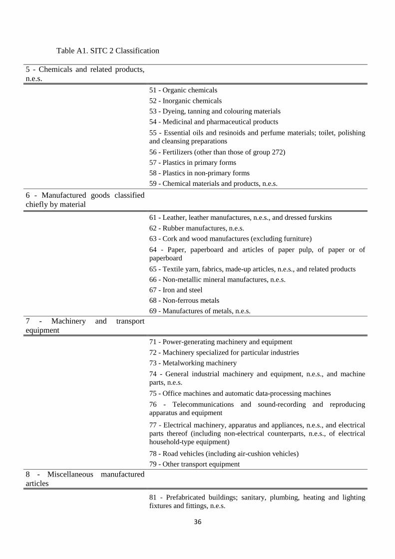
Table A1. SITC 2 Classification

5 - Chemicals and related products, n.e.s.

51 - Organic chemicals 52 - Inorganic chemicals 53 - Dyeing, tanning and colouring materials 54 - Medicinal and pharmaceutical products

55 - Essential oils and resinoids and perfume materials; toilet, polishing and cleansing preparations

56 - Fertilizers (other than those of group 272) 57 - Plastics in primary forms 58 - Plastics in non-primary forms 59 - Chemical materials and products, n.e.s. 6 - Manufactured goods classified chiefly by material

61 - Leather, leather manufactures, n.e.s., and dressed furskins 62 - Rubber manufactures, n.e.s. 63 - Cork and wood manufactures (excluding furniture)

64 - Paper, paperboard and articles of paper pulp, of paper or of paperboard

65 - Textile yarn, fabrics, made-up articles, n.e.s., and related products 66 - Non-metallic mineral manufactures, n.e.s. 67 - Iron and steel 68 - Non-ferrous metals 69 - Manufactures of metals, n.e.s. 7 - Machinery and transport equipment

71 - Power-generating machinery and equipment 72 - Machinery specialized for particular industries 73 - Metalworking machinery

74 - General industrial machinery and equipment, n.e.s., and machine parts, n.e.s.

75 - Office machines and automatic data-processing machines

76 - Telecommunications and sound-recording and reproducing apparatus and equipment

77 - Electrical machinery, apparatus and appliances, n.e.s., and electrical parts thereof (including non-electrical counterparts, n.e.s., of electrical household-type equipment)

78 - Road vehicles (including air-cushion vehicles) 79 - Other transport equipment 8 - Miscellaneous manufactured articles

81 - Prefabricated buildings; sanitary, plumbing, heating and lighting fixtures and fittings, n.e.s.

37

82 - Furniture, and parts thereof; bedding, mattresses, mattress supports, cushions and similar stuffed furnishings

83 - Travel goods, handbags and similar containers 84 - Articles of apparel and clothing accessories 85 - Footwear

87 - Professional, scientific and controlling instruments and apparatus, n.e.s.

88 - Photographic apparatus, equipment and supplies and optical goods, n.e.s.; watches and clocks

89 - Miscellaneous manufactured articles, n.e.s. Source : United Nations, 2009.

38

Table A.2. Cumulation Rules

Cumulation Rules. Mediterranean Countries

Algeria (01.09.2005)

Euro-Mediterranean Association Agreement, OJ L 265, 10.10.2005

Protocol No 6

OJ L 297 of 15.11.2007

Bilateral, diagonal and full cumulation

Tunisia (01.03.1998)

Euro-Mediterranean Association Agreement , OJ L 97, 30.03.1998, p.2.

Protocol No 4

OJ L 260 of 21.9.2006

Bilateral, diagonal and full cumulation

Morocco (01.03.2000)

Euro-Mediterranean Association Agreement, OJ L 70, 18.03.2000, p.2

Protocol No 4

OJ L 336 of 21.12.2005

Bilateral, diagonal and full cumulation

Israel (01.06.2000)

Euro-Mediterranean Association Agreement , OJ L 147, 21.06.2000, p.3

Protocol No 4

OJ L 20 of 24.1.2006

Bilateral and diagonal cumulation

Palestinian Authority of the West Bank and the Gaza Strip (01.07.1997)

Euro-Mediterranean Interim Association Agreement , OJ L 187, 16.07.1997, p.3.

Protocol No 3

OJ L 187 of 16.07.1997

Bilateral cumulation

Egypt (01.06.2004)

Mediterranean Association Agreement, OJ L304 of 30.09.2004, p.39

Protocol No 4

OJ L 73 of 13.3.2006

Bilateral and diagonal cumulation

Jordan (01.05.2002)

Euro-Mediterranean Association Agreement, OJ L 129, 15.05.2002, p.3.

Protocol No 3

OJ L 209 of 31.7.2006

Bilateral and diagonal cumulation

Lebanon (01.03.2003 Interim Agreement)

Euro-Mediterranean Association Agreement, OJ L 143, 30.05.2006, p.2.

Protocol No 4

OJ L 143, 30.05.2006, p. 73

Bilateral cumulation

Syria (01.07.1977)

Cooperation Agreement, OJ L 269, 27.09.1978, p.2.

Protocol No 2

Bilateral cumulation

Source: http://ec.europa.eu/taxation_customs/customs/customs_duties/rules_origin/preferential/article_779_en.htm#paneuro.