Economic Impact Analysis for the Final Vegetable Oil Processing ...

United States Office Of Air Quality EPA-452/R-01-005Environmental Protection Planning And Standards January 2001Agency Research Triangle Park, NC 27711 FINAL REPORT

Air

Economic Impact Analysis for the FinalVegetable Oil Processing NESHAP

Final Report

Economic Impact Analysis for the Proposed Vegetable Oil

Processing NESHAP

U.S. Environmental Protection AgencyOffice of Air Quality Planning and Standards

Innovative Strategies and Economics Group, MD-15Research Triangle Park, NC 27711

Prepared Under Contract By:

Research Triangle InstituteCenter for Economics Research

Research Triangle Park, NC 27711

January 2001

This report has been reviewed by the Emission Standards Division of the Office of Air QualityPlanning and Standards of the United States Environmental Protection Agency and approved forpublication. Mention of trade names or commercial products is not intended to constituteendorsement or recommendation for use. Copies of this report are available through the LibraryServices (MD-35), U.S. Environmental Protection Agency, Research Triangle Park, NC 27711, orfrom the National Technical Information Services 5285 Port Royal Road, Springfield, VA 22161.

iii

CONTENTS

Section Page

Executive Summary . . . . . . . . . . . . . . . . . . . . . . . . . . . . . . . . . . . . . . . . . . . . . ES-1

1 Introduction . . . . . . . . . . . . . . . . . . . . . . . . . . . . . . . . . . . . . . . . . . . . . . . . . . . . 1-1

1.1 Scope and Purpose . . . . . . . . . . . . . . . . . . . . . . . . . . . . . . . . . . . . . . . . . 1-1

1.2 Organization of the Report . . . . . . . . . . . . . . . . . . . . . . . . . . . . . . . . . . . 1-2

2 Industry Profile . . . . . . . . . . . . . . . . . . . . . . . . . . . . . . . . . . . . . . . . . . . . . . . . . . 2-1

2.1 Production . . . . . . . . . . . . . . . . . . . . . . . . . . . . . . . . . . . . . . . . . . . . . . . 2-2

2.2 Market Data . . . . . . . . . . . . . . . . . . . . . . . . . . . . . . . . . . . . . . . . . . . . . . 2-42.2.1 Quantity Data . . . . . . . . . . . . . . . . . . . . . . . . . . . . . . . . . . . . . . . 2-42.2.2 Baseline and Historical Price Data . . . . . . . . . . . . . . . . . . . . . . . 2-6

2.3 Affected Producers . . . . . . . . . . . . . . . . . . . . . . . . . . . . . . . . . . . . . . . . 2-102.3.1 Manufacturing Facilities . . . . . . . . . . . . . . . . . . . . . . . . . . . . . 2-102.3.2 Companies . . . . . . . . . . . . . . . . . . . . . . . . . . . . . . . . . . . . . . . . 2-21

2.4 Consumption and Uses of Vegetable Oils and Meals . . . . . . . . . . . . . 2-242.4.1 Vegetable Oil Consumption and Uses . . . . . . . . . . . . . . . . . . . 2-242.4.2 Oilseed Meal Consumption and Uses . . . . . . . . . . . . . . . . . . . 2-26

3 Engineering Cost Analysis . . . . . . . . . . . . . . . . . . . . . . . . . . . . . . . . . . . . . . . . . 3-1

3.1 Control Options and Costs . . . . . . . . . . . . . . . . . . . . . . . . . . . . . . . . . . . 3-23.1.1 Control Options . . . . . . . . . . . . . . . . . . . . . . . . . . . . . . . . . . . . . 3-23.1.2 Control Costs . . . . . . . . . . . . . . . . . . . . . . . . . . . . . . . . . . . . . . . 3-5

3.2 National Emissions Reductions and Compliance Costs . . . . . . . . . . . . 3-8

iv

4 Economic Impact Analysis . . . . . . . . . . . . . . . . . . . . . . . . . . . . . . . . . . . . . . . . 4-1

4.1 Economic Analysis Inputs . . . . . . . . . . . . . . . . . . . . . . . . . . . . . . . . . . . 4-14.1.1 Producer Characterization . . . . . . . . . . . . . . . . . . . . . . . . . . . . . 4-14.1.2 Vegetable Oil and Meal Markets . . . . . . . . . . . . . . . . . . . . . . . . 4-24.1.3 Regulatory Control Costs . . . . . . . . . . . . . . . . . . . . . . . . . . . . . . 4-2

4.2 Economic Impact Methodology . . . . . . . . . . . . . . . . . . . . . . . . . . . . . . . 4-5

4.3 Economic Model Assumptions . . . . . . . . . . . . . . . . . . . . . . . . . . . . . . . 4-84.3.1 Operational Assumptions . . . . . . . . . . . . . . . . . . . . . . . . . . . . . . 4-84.3.2 Numerical Assumptions . . . . . . . . . . . . . . . . . . . . . . . . . . . . . . . 4-9

4.3.2.1 Elasticity Assumptions . . . . . . . . . . . . . . . . . . . . . . . . 4-94.3.2.2 Allocation of Compliance Costs to Oils and Meals . 4-114.3.2.3 Allocation of Seed Costs to Oils and Meals . . . . . . . 4-11

4.4 Economic Impact Results . . . . . . . . . . . . . . . . . . . . . . . . . . . . . . . . . . . 4-124.4.1 Market-Level Results . . . . . . . . . . . . . . . . . . . . . . . . . . . . . . . . 4-124.4.2 Industry-Level Results . . . . . . . . . . . . . . . . . . . . . . . . . . . . . . . 4-124.4.3 Social Costs of the Regulation . . . . . . . . . . . . . . . . . . . . . . . . . 4-16

5 Small Business Impacts . . . . . . . . . . . . . . . . . . . . . . . . . . . . . . . . . . . . . . . . . . . 5-1

6 Assumptions and Limitations of the Economic Model . . . . . . . . . . . . . . . . . . . 6-1

References . . . . . . . . . . . . . . . . . . . . . . . . . . . . . . . . . . . . . . . . . . . . . . . . . . . . . . . . . . . R-1

Appendix A Economic Model of The U.S. Vegetable Oil and Meal Markets . . . . . A-1

Appendix B Estimates of the Demand and Supply Elasticities for Vegetable Oilsand Meals . . . . . . . . . . . . . . . . . . . . . . . . . . . . . . . . . . . . . . . . . . . . . . . . B-1

Appendix C Economic Model Sensitivity Analysis . . . . . . . . . . . . . . . . . . . . . . . . . . C-1

v

LIST OF FIGURES

Number Page

2-1 Simplified Solvent Extraction Process for Vegetable Oils . . . . . . . . . . . . . . . . 2-22-2 U.S. Consumption of Fats and Oils by Use, 1995 . . . . . . . . . . . . . . . . . . . . . . 2-262-3 U.S. Processed Feeds by Type, 1995 . . . . . . . . . . . . . . . . . . . . . . . . . . . . . . . . 2-28

4-1 Supply Curve for a Representative Affected Facility . . . . . . . . . . . . . . . . . . . . 4-64-2 Market Equilibrium Without and With Regulation . . . . . . . . . . . . . . . . . . . . . . 4-7

vi

LIST OF TABLES

Number Page

2-1 Summary of Output Shares Relative to Input Volumes (short tons) . . . . . . . . . 2-32-2 U.S. Inventories, Production, Foreign Trade, and Apparent Consumption of

Vegetable Oils by Market: 1995 (short tons) . . . . . . . . . . . . . . . . . . . . . . . . . . 2-52-3 Prices of Vegetable Oils, 1990-1996 (cents/lb) . . . . . . . . . . . . . . . . . . . . . . . . . 2-72-4 Prices of Meal and Similar Products, 1990-1996 (cents/lb) . . . . . . . . . . . . . . . 2-82-5 Prices of Oilseeds: 1990-1996 (cents/lb) . . . . . . . . . . . . . . . . . . . . . . . . . . . . . 2-92-6(a) Solvent Extraction Corn Oil Manufacturing Facilities and Locations . . . . . . . 2-112-6(b) Solvent Extraction Cottonseed Oil Manufacturing Facilities

and Locations . . . . . . . . . . . . . . . . . . . . . . . . . . . . . . . . . . . . . . . . . . . . . . . . . . 2-122-6(c) Solvent Extraction Soybean Oil Manufacturing Facilities

and Locations . . . . . . . . . . . . . . . . . . . . . . . . . . . . . . . . . . . . . . . . . . . . . . . . . . 2-142-6(d) Solvent Extraction Other Vegetable Oil Manufacturing

Facilities and Locations . . . . . . . . . . . . . . . . . . . . . . . . . . . . . . . . . . . . . . . . . . 2-182-7 Baseline Vegetable Oil Volumes and Shares by Market and Extraction

Method: 1995 (short tons) . . . . . . . . . . . . . . . . . . . . . . . . . . . . . . . . . . . . . . . . 2-202-8 Sales and Employment Data for Solvent Extraction Vegetable

Oil Companies . . . . . . . . . . . . . . . . . . . . . . . . . . . . . . . . . . . . . . . . . . . . . . . . . 2-222-9 Per Capita Consumption of Vegetable Oils: 1990-1996 (lbs) . . . . . . . . . . . . 2-252-10 Per Capita Consumption of Meal Products: 1990-1996 (lbs) . . . . . . . . . . . . . 2-27

3-1 Summary of Control Technologies Assigned to Model Plants . . . . . . . . . . . . . 3-43-2 Cost Estimates for MACT Floor Control Technologies for

Each Model Plant (1995 dollars) . . . . . . . . . . . . . . . . . . . . . . . . . . . . . . . . . . . . 3-63-3 Incremental Cost Estimates for Above-the-MACT-Floor Control

Technologies for Each Model Plant (1995 dollars) . . . . . . . . . . . . . . . . . . . . . . 3-93-4 Summary of National Emissions and Costs for the MACT Floor and

Above-the- MACT-Floor Control Scenarios (1995 dollars) . . . . . . . . . . . . . . 3-10

4-1 Summary of Baseline Vegetable Oil and Meal Values: 1995 . . . . . . . . . . . . . . 4-34-2 Distribution of Facility-Level Compliance Cost-to-Sales Ratios: 1995 . . . . . . 4-44-3 Elasticity Estimates Used in the Economic Impact Analysis . . . . . . . . . . . . . . 4-10

vii

4-4 Summary of Market-Level Impacts of Vegetable Oil Production NESHAP: 1995 . . . . . . . . . . . . . . . . . . . . . . . . . . . . . . . . . . . . . . 4-13

4-5 Summary of Industry-Level Impacts of Vegetable Oil ProductionNESHAP: 1995 . . . . . . . . . . . . . . . . . . . . . . . . . . . . . . . . . . . . . . . . . . . . . . . . 4-15

4-6 Summary of Distributional Industry Impacts of Vegetable Oil Production NESHAP: 1995 . . . . . . . . . . . . . . . . . . . . . . . . . . . . . . . . . . . . . . . . . . . . . . . . 4-17

4-7 Distribution of the Social Costs Associated with the Vegetable Oil ProductionNESHAP: 1995 . . . . . . . . . . . . . . . . . . . . . . . . . . . . . . . . . . . . . . . . . . . . . . . . 4-18

5-1 Summary Data for Small Companies: 1995 . . . . . . . . . . . . . . . . . . . . . . . . . . . 5-35-2 Capacity and Compliance Cost Comparisons for Small and

Large Companies: 1995 . . . . . . . . . . . . . . . . . . . . . . . . . . . . . . . . . . . . . . . . . . 5-45-3 Summary of Cost-to-Sales Ratios for the Vegetable Oil

NESHAP: 1995 (%) . . . . . . . . . . . . . . . . . . . . . . . . . . . . . . . . . . . . . . . . . . . . . 5-55-4 Distribution of Cost-to-Sales Ratios for the Vegetable Oil

NESHAP: 1995 . . . . . . . . . . . . . . . . . . . . . . . . . . . . . . . . . . . . . . . . . . . . . . . . . 5-65-5 Summary of Company Cost-to-Sales Ratios for Companies That

Own Cottonseed Facilities: 1995 (%) . . . . . . . . . . . . . . . . . . . . . . . . . . . . . . . . 5-85-6 Distribution of Cost-to-Sales Ratios for Companies That Own Cottonseed

Facilities: 1995 . . . . . . . . . . . . . . . . . . . . . . . . . . . . . . . . . . . . . . . . . . . . . . . . . 5-95-7 Summary of Facility Cost-to-Sales Ratios for Cottonseed

Facilities: 1995 (%) . . . . . . . . . . . . . . . . . . . . . . . . . . . . . . . . . . . . . . . . . . . . . 5-105-8 Summary of Small Business Impacts of Vegetable Oil Production

NESHAP: 1995 . . . . . . . . . . . . . . . . . . . . . . . . . . . . . . . . . . . . . . . . . . . . . . . . 5-12

ix

LIST OF ACRONYMS

2SLS two-stage least squares

AC annualized capital investment

CBI confidential business information

CSRs cost-to-sales ratios

EIA economic impact analysis

FTEs full-time equivalents

GDP gross domestic product

HAPs hazardous air pollutants

HHIs Herfindahl-Hirschman indexes

ISEG Innovative Strategies and Economics Group

LP lost production

LDAR leak detection and repair

LPC lost production costs (operating costs and foregone profits incurredwhile the plant is shut down to install capital)

MACT maximum achievable control technology

MRR monitoring, recordkeeping, and reporting costs

NAICS North American Industry Classification System

NESHAP National Emission Standard for Hazardous Air Pollutants

O&M operating and maintenance costs

OAQPS Office of Air Quality Planning and Standards

OLS ordinary least squares

RFA Regulatory Flexibility Act

SBA Small Business Administration

x

SBREFA Small Business Regulatory Enforcement Fairness Act of 1996

SIC Standard Industrial Classification

SRC solvent recovery credit

tpd tons per day

tpy tons per year

USDA U.S. Department of Agriculture

VOCs volatile organic compounds

ES-1

EXECUTIVE SUMMARY

This report analyzes the economic impacts of an air pollution regulation to reduceemissions of hexane, which is a solvent, generated in the production of crude vegetable oilsand meals. Hexane is a hazardous air pollutant (HAP). This analysis presents the economicimpacts of two regulatory alternatives. The first alternative is the MACT floor, and the EPAis promulgating this regulatory alternative. The economic impact results are also presentedfor an above-the-MACT-floor alternative, and these results are presents for comparisonpurposes only.

How do emissions of HAPs occur in the production of vegetable oils and meals?

Emissions of HAPs from the production of vegetable oil and meal originate from thetransfer and storage of solvent (hexane); potential leaks of solvent from piping and tanks;process vents (solvent recovery section, meal dryer, and meal cooler); and solvent retained inthe crude oil or meal after processing.

Which markets are affected by the regulation?

The affected markets are those for crude soybean oil and meal, crude cottonseed oiland meal, crude corn oil and corn germ meal, and other types of crude vegetable oil and meal. Other types include safflower, sunflower, flaxseed, canola, and peanut oils and meals. Themarkets for refined vegetables oils are not directly affected.

Which producers will be affected?

In 1995, the baseline year of the analysis, the affected producers are the 106 vegetableoil processing facilities that produce vegetable oil and meal using a solvent extractionprocess. Both new and existing producers will be affected. A total of 31 companies areidentified as owners of these vegetable oil and meal plants.

How many small businesses will be affected?

Based on Small Business Administration (SBA) definitions, 15 small companiesowned and operated 21 facilities, or 20 percent of all solvent extraction facilities in 1995.

ES-2

What are the compliance costs associated with the regulation?

The costs that each facility will incur include capital costs; operating and maintenancecosts; monitoring, recordkeeping, and reporting costs; and lost production costs (operatingcosts and lost profits incurred while process changes are implemented). On an annualizedbasis, the compliance costs for plants operating in 1995 and for three plants that beganoperation in 1996 were estimated at $12.3 million with the maximum achievable controltechnology (MACT) floor scenario and $204.6 million with the more stringent above-the-MACT-floor scenario.

What are the expected emissions reductions as a result of the regulation?

The U.S. Environmental Protection Agency (EPA) estimates that a 25 percentreduction in emissions will be achieved with the MACT floor scenario, and a 43 percentreduction in emissions will be achieved with the above-the-MACT-floor scenario.

How large are the compliance costs relative to sales for the entire industry?

Cost-to-sales ratios (CSRs) were calculated at the facility level by dividing theregulatory compliance costs by facility revenue. For the MACT floor scenario, 104 of the106 facilities have CSRs below 1 percent, two have CSRs from 1 to 2 percent, and no facilityhas a CSR above 2 percent. For the above-the-floor scenario, 17 facilities have CSRs below1 percent, 44 have CSRs from 1 to 2 percent, and 45 have CSRs above 2 percent.

How do the compliance costs relative to sales compare for small businesses?

Under the floor scenario, average CSRs are 0.30 percent for small companies and0.04 percent for large companies. Under the above-the-floor scenario, average CSRs are 2.97percent for small companies and 0.45 percent for large companies.

What are the overall expected effects on prices, output, and revenues?

Under the floor scenario, prices for individual vegetable oils and meals are expectedto increase by one-half of 1 percent or less, output is expected to decline by approximatelyone-third of 1 percent or less, and revenues are expected to increase by one-tenth of 1percent. Under the above-the-floor scenario, prices for vegetable oils and meals are expectedto increase by 2 to 13 percent under the above-the-floor scenario, output is expected todecline by 1 to 6 percent, and revenues are expected to increase by 4 percent.

ES-3

What are the predicted effects of the regulation on employment in the industry?

Employment is expected to decrease by 12 individuals under the floor scenario and by350 individuals under the above-the-floor scenario.

Are any facilities predicted to close under the regulation?

No product-line or facility closures are predicted with the floor option. Sixproduct-line closures and three facility closures are predicted with the above-the-floor option.

Will this regulation pose a significant impact on a substantial number of small entities?

No. Under the floor scenario with lost production costs, the screening analysis(CSRs) and the market impact analysis do not show a significant impact on a substantialnumber of small entities. The potential for negative impacts is greater under the above-the-floor scenario.

How have economic conditions changed in the affected industries since 1995, thebaseline year of the analysis?

The markets for oilseeds, oils, and meals exhibit a great deal of volatility over time. Since 1995, the prices of the primary oilseeds and similar inputs used in the production ofvegetable oils and meals generally increased, while the prices of crude vegetables and mealsgenerally decreased. However, the magnitude of the compliance costs relative to sales didnot increase substantially using 1999 data compared to using 1995 data. In 2000, economicconditions in these industries have generally improved.

1-1

SECTION 1

INTRODUCTION

The U.S. Environmental Protection Agency (referred to as EPA or the Agency) is

developing an air pollution regulation for reducing emissions of hexane generated in the

production of crude vegetable oils and related products. These products include crude

soybean oil and meal, crude cottonseed oil and meal, crude corn oil and corn germ meal, and

crude specialty vegetable oils and meals. The regulation does not apply to facilities that

refine crude vegetable oil. EPA’s Office of Air Quality Planning and Standards (OAQPS) is

developing the National Emission Standard for Hazardous Air Pollutants (NESHAP) under

Section 112 of the Clean Air Act Amendments of 1990 to limit these emissions. The

Innovative Strategies and Economics Group (ISEG) has developed this economic impact

analysis (EIA) to support the evaluation of impacts associated with the regulatory alternatives

considered for this NESHAP. This report presents economic impacts of the maximum

achievable control technology (MACT) floor regulatory alternative promulgated by the EPA

and economic impacts for an above-the-MACT-floor regulatory alternative for comparison

purposes.

1.1 Scope and Purpose

This report evaluates the economic impacts of pollution control requirements in the

production of vegetable oils and related products that are designed to reduce releases of

hazardous air pollutants (HAPs) into the atmosphere. The Clean Air Act’s purpose is to

protect and enhance the quality of the nation’s air resources (Section 101(b)). Section 112 of

the Clean Air Act Amendments of 1990 establishes the authority to set national emissions

standards for 189 HAPs. Emissions of HAPs from the production of vegetable oil and meal

originate from the transfer and storage of solvent (hexane); potential leaks of solvent from

piping and tanks; process vents (solvent recovery section, meal dryer, and meal cooler); and

solvent retained in the crude oil or meal after processing (Midwest Research Institute, 1995).

1Most vegetable oil production processes use solvent extraction. Mechanical extraction accounts for less than 6percent of production of vegetable oils.

1-2

The NESHAP will apply to all existing and new major sources that manufacture

vegetable oil and related products using solvent extraction processes.1 A major source is

defined as a stationary source or group of stationary sources located within a contiguous area

and under common control that emits, or has the potential to emit, 10 tons or more of any one

HAP or 25 tons or more of any combination of HAPs. In 1995, an estimated 106 processing

facilities produce crude vegetable oil and related products in the United States using solvent

extraction processes. Some of these facilities process multiple oilseed types (e.g., soybean,

cottonseed, corn, safflower, sunflower, canola, peanut). Based on 1995 emissions data, EPA

has determined that all of these facilities are major sources of HAPs.

To reduce emissions of HAPs, the Agency establishes MACT standards. The term

“MACT floor” refers to the minimum control technology on which MACT standards can be

based. For existing major sources, the MACT floor is the average emissions limitation

achieved by the best performing 12 percent of sources (if there are 30 or more sources in the

category or subcategory). The MACT can be more stringent than the floor, considering costs,

nonair quality health and environmental impacts, and energy requirements. The estimated

costs for individual plants to comply with the MACT are inputs into the economic impact

analysis presented in this report.

This report analyzes the economic effects of the MACT standard on existing sources.

The MACT standard is the same for both new and existing soybean plants, which contribute

the majority of HAP releases, but slightly more stringent for new plants that process other

oilseed types. However, the economic impacts of the regulation on new sources of all types

are expected to be minimal. Newly installed equipment is expected to be already in

compliance with the MACT standard and no add-on control equipment will be necessary.

Therefore, this report does not explicitly analyze the impact of the regulation on new sources.

However, because the baseline year of the analysis is 1995, this report describes changes in

economic conditions of the affected industries since that time.

1.2 Organization of the Report

The remainder of this report is divided into five sections that describe the

methodology and present results of this analysis:

1-3

� Section 2 provides a summary profile of the production of crude vegetable oilsand related products. It presents data on market volumes and prices,manufacturing plants, and the companies that own and operate these plants.

� Section 3 reviews the regulatory control options and associated costs ofcompliance. This section is based on EPA’s engineering analysis conducted insupport of the NESHAP.

� Section 4 details the methodology for assessing the economic impacts of theNESHAP and the results of the analysis, which include market, industry, andsocial cost impacts.

� Section 5 provides the Agency’s analysis of the regulation’s impact on smallbusinesses.

� Section 6 describes the assumptions used in this analysis.

In addition to these sections, Appendix A describes the economic model used to predict the

economic impacts of the NESHAP, Appendix B provides information on the elasticities of

demand and supply used in the model, and Appendix C provides the results of sensitivity

analyses on the model assumptions.

1These minor products are not described as part of this summary profile because available data are insufficientto characterize them.

2-1

SECTION 2

INDUSTRY PROFILE

Most crude vegetable oil and related products are produced using solvent extraction

processes (affected facilities), although a small proportion is still produced using mechanical

or hydraulic extraction processes (unaffected facilities). The affected products produced by

vegetable oil facilities are classified in the following North American Industry Classification

System (NAICS) codes:

� NAICS 311221, Wet Corn Products and NAICS 311211 Flour and Other GrainMill Products—corn oil and corn germ meal;

� NAICS 311222, Soybean Products—soybean oil and soybean meal; and

� NAICS 311223, Other Oilseed Products—oils and meals of cottonseed, canola,flaxseed, rice, safflower, sunflower, and other oilseeds.

In addition to these primary products, other minor products, such as hulls, linters, and

lecithin, are produced as well.1

This section provides a summary profile of the vegetable oil and related products

industries as background information for understanding the technical and economic aspects

of the industries. Section 2.1 presents a brief overview of the production process.

Section 2.2 provides market data on U.S. production, consumption, foreign trade, and prices.

Section 2.3 describes the affected U.S. processing facilities and the companies that own

them. Finally, Section 2.4 provides data on the consumers and uses of vegetable oils and

related products.

2.1 Production

Figure 2-1 shows a simplified process diagram for vegetable oils and related products.

Oilseeds, such as soybeans and cottonseed, or similar inputs, such as peanuts, rice, and corn

2-2

Preparation

Oil Extraction

Solvent Recovery

Cake, Meal, andOther Products

Crude Oil Product

Desolventizing/Toasting/Drying/

Cooling

Oilseeds or Similar Inputs

Hexane

Oilseeds fromPreparation

Solvent and Extracted Flakes Solvent and Crude Oil RecycledSolvent

Hulls

Hexane

RecycledSolvent

Figure 2-1. Simplified Solvent Extraction Process for Vegetable Oils

germ, are dehulled, cracked and flaked, and prepared for oil extraction. Hexane is added to

dissolve the oil in the prepared oilseed or similar input and then recovered in a desolventizing

(evaporation) process. Recovered hexane is then recycled for reuse in the process.

Crude oil products produced at these facilities are then transferred to a refining

facility where they are prepared for human consumption. Meal products are either further

processed into a variety of products for human consumption or prepared for use in animal

feeds.

Based on the data, it appears that facilities produce relatively fixed proportions of

their outputs to the oilseeds or similar inputs. Table 2-1 shows the average shares of oil

production and meal production volumes relative to oilseed volumes based on U.S.

Department of Agriculture (USDA) data for the years 1975 through 1996 and on the EPA

facility database for 1995. Soybeans generate an average of 18.2 percent oil and 79.2 percent

meal, with 2.6 percent shrink or waste by weight based on USDA data. These numbers are

2-3

similar to the figures provided by David Ailor (1998) of the National Oilseed Processors

Association (18.5 percent oil, 79 percent meal, 2.5 percent shrink and waste) and based on

the EPA facility database (19.0 percent oil; 74.5 percent meal; and 6.5 percent shrink, waste,

and hulls). Based on USDA data, cottonseed generated an average of 16.2 percent oil and

45.7 percent meal, with the remainder going to other products, and based on the EPA facility

database, cottonseed generated an average of 16.4 percent oil and 46.0 percent meal. USDA

does not report comparable figures for corn germ or the other oilseed types. However, based

on the EPA facility database, corn germ is on average 43.1 percent oil and 56.6 percent meal.

All other oilseeds are on average 39.5 percent oil and 57.6 percent meal.

Table 2-1. Summary of Output Shares Relative to Input Volumes (short tons)

TotalCrushedVolume

Oil Product Meal Product

ProductionVolume

Share(%)

ProductionVolume

Share(%)

USDA (1975 - 1996)a

Soybean

Mean 29,991,290 5,472,871 18.2% 23,740,258 79.2%

Standard deviation 7,451,987 1,423,299 0.45% 5,950,354 1.16%

Cottonseed

Mean 3,636,076 588,727 16.2% 1,660,773 45.7%

Standard deviation 482,524 94,383 0.96% 281,226 2.65%

EPA Facility Database(1995)b

Corn 2,477,695 1,066,819 43.1% 1,401,546 56.6%

Cottonseed 3,794,066 622,308 16.4% 1,744,562 46.0%

Soybean 41,920,179 7,968,264 19.0% 31,225,572 74.5%

All other 2,601,092 1,026,335 39.5% 1,497,886 57.6%

a The USDA reports total crushed volumes based on a marketing year beginning September 1. These volumeshave been adjusted to reflect a marketing year beginning October 1 to be consistent with reported oil andmeal production.

b Oil and meal product quantities for seven facilities have been adjusted to be consistent with reported totalcrushed volumes.

Source: U.S. Department of Agriculture. 1997c. Oil Crops Situation and Outlook Yearbook. Washington,DC: Government Printing Office.

2-4

Because the calculated percentages based on USDA data were fairly constant over

time and because the major trade associations verified that these percentages remain constant,

fixed production proportions are assumed in the EIA. Thus, predicted changes in oil and

meal production due to the effects of the regulation were verified against these percentages as

part of the EIA.

2.2 Market Data

This section presents baseline 1995 data for production, exports, imports, and

apparent consumption of each of the three primary oil products and their associated meal

products, as well as other vegetable oils and meals combined. Because the prices for these

products are volatile, both historical and recent price data are included for the major outputs

and the oilseed inputs.

2.2.1 Quantity Data

Table 2-2 provides baseline 1995 data on production, exports, imports, and apparent

consumption of corn oil, cottonseed oil, soybean oil, all other vegetable oils combined, corn

germ meal, cottonseed meal, soybean meal, and all other meals combined, as reported by the

USDA and Department of Commerce.

In 1995, soybean oil accounted for 74 percent of all vegetable oil production.

Approximately 15 percent of soybean oil production was exported. Even greater percentages

of the other oils were exported: 37 percent of corn oil, 23 percent of cottonseed oil, and

62 percent of all other vegetable oils combined. Small quantities of corn, cottonseed, and

soybean oil were imported, but nearly half of all other vegetable oils combined were

imported. Most of this quantity was canola oil, which is currently produced in only small

quantities in the United States.

As with the oil products, soybean meal made up the majority of meal production,

accounting for 92 percent of all meals combined in 1995. Approximately 19 percent of

soybean meal was exported, compared to 5 percent of cottonseed meal and 13 percent of all

other meals. Production and import data were unavailable for corn germ meal. The United

States imports insignificant quantities of soybean and cottonseed meal but imports

approximately half of all other meals (canola, flaxseed, and sunflower).

2-5

Table 2-2. U.S. Inventories, Production, Foreign Trade, and Apparent Consumption ofVegetable Oils by Market: 1995 (short tons)

MarketBeginningInventory Production Imports Exports

EndingInventory

ApparentConsumptiona

Oil products

Corn oil 45,091 1,121,703 4,495 415,270 98,203 657,816

Cottonseed oil 57,370 645,925 106 147,281 47,424 508,697

Soybean oil 527,616 7,818,128 13,616 1,143,544 704,447 6,511,369

All other vegetableoilsb

135,042 1,015,792 529,125 632,625 146,792 900,542

Total, oils 765,118 10,601,548 547,341 2,338,719 996,865 8,578,423

Meal products

Corn germ meal NA NA NA 61,950 NA NA

Cottonseed meal 94,900 1,826,100 0 89,700 21,200 1,810,100

Soybean meal 241,117 33,340,037 65,405 6,491,570 290,100 26,864,889

All other mealsc 16,512 1,091,571 936,570 138,469 16,512 1,889,673

Total, meals 352,529 36,257,708 1,001,975 6,781,688 327,812 30,564,662

All other productsd NA 3,781,800 NA NA NA NA

a Apparent Consumption = Beginning Inventory + Production + Imports – Exports – Ending Inventoryb Includes canola, flaxseed, peanut, safflower, and sunflower volumes.c Includes canola, flaxseed, and sunflower volumes.d Includes cottonseed hulls, lecithin, cottonseed linters, and soybean hulls.

Sources: U.S. Department of Agriculture, Economic Research Service. Oil Crops Yearbook. [computer file]. Last updated January 1998.

U.S. Department of Commerce. 1996a. 1995 Current Industrial Reports—Fats and Oils: OilseedCrushings. M20J. Washington, DC: Government Printing Office.

U.S. Bureau of the Census. 1998a. U.S. Exports History: Historical Summary 1993-1997 on CD-ROM [machine readable data file]. Washington, DC: Bureau of the Census.

U.S. Bureau of the Census. 1998b. U.S. Imports History: Historical Summary 1993-1997 on CD-ROM [machine readable data file]. Washington, DC: Bureau of the Census.

2-6

All other vegetable oil products totaled 3.8 million tons in 1995. These include

products such as hulls, lecithin, and cottonseed linters. Because of insufficient data, these

products are not included in the EIA.

2.2.2 Baseline and Historical Price Data

Historical price data for 1990 through 1999 for crude vegetable oils are presented in

Table 2-3, with the 1995 baseline year of analysis in boldface. While the prices for corn,

cottonseed, and soybean enter the model individually, the prices of canola, flaxseed, peanut,

safflower, and sunflower are combined into a weighted average price for all other vegetable

oils (see Table 4-1). Prices of oil tend to fluctuate greatly from year to year and appear to

have peaked in 1994 for many of the oils and then fallen in 1995 and each year since then.

The decrease in prices is attributable primarily to changes in the international markets for oil.

In particular, crushing capacities in South America and Europe have expanded, thus reducing

the demand for vegetable oil exports to these countries (USDA, 1999c).

Prices for oilseed meal and similar products are listed in Table 2-4 for 1990 through

1999, with the baseline 1995 data again in boldface. As with oil prices, these prices fluctuate

greatly from year to year. For these products, prices appear to have peaked in 1993, fallen in

1994 and 1995, peaked again in 1996 and 1997, and then fallen drastically in 1998 and 1999.

As with the prices for vegetable oils, these decreases are most likely attributable to a

reduction in export demand for meals. Thus, for both vegetable oils and meals, prices

received by vegetable oil processors were higher in 1995 than in recent years.

A large percentage of the costs of producing vegetable oils and meals is the cost of

the raw agricultural inputs. In Table 2-5, their prices are presented for 1990 through 1999,

with baseline 1995 data in boldface. Because these are agricultural commodities, acres

planted and weather conditions influence the output in any given year; thus, prices tend to be

volatile. In 1995, prices of oilseeds and similar inputs were substantially higher than in 1999

with the exception of cottonseed. Thus, while output prices for most vegetable oils and

meals have fallen recently for most oilseed types, the cost of the primary input has fallen also.

The situation for cottonseed is different than for the other oilseeds because cottonseed is

being used increasingly as a dairy cow feed.

2-7

Table 2-3. Prices of Vegetable Oils, 1990-1996 (cents/lb)

Corn Cottonseed Soybean Canolaa Flaxseed Peanut Safflower Sunflower

1990 25.40 23.90 23.40 24.40 40.10 45.70 55.10 22.10

1991 28.40 20.70 20.30 21.30 34.50 38.06 49.20 23.40

1992 24.00 21.40 19.30 20.30 30.70 25.03 60.00 22.90

1993 21.80 26.00 22.70 23.70 31.70 34.10 70.00 26.80

1994 27.30 27.10 27.90 28.90 32.50 45.91 59.00 31.10

1995 26.60 26.80 26.80 27.80 35.00 41.57 59.00 28.90

1996 26.50 25.90 23.80 24.80 37.10 40.20 59.00 24.66

1997 24.85 26.51 23.27 24.27 36.25 47.20 59.00 23.45

1998 30.33 31.03 25.73 26.73 36.00 47.21 59.00 24.24

1999 23.36 23.95 17.60 18.60 36.00 38.25 59.00 19.00

a USDA does not report a crude canola oil price; thus, it was approximated as one cent per pound over the soybean oil price (Marine, 1999).

Sources: U.S. Department of Agriculture. 2000. Agricultural Statistics 2000. Washington, DC: Government Printing Office.

U.S. Department of Agriculture, Economic Research Service. 1999b. Oil Crops Yearbook. [computer file]. Last updatedNovember 1999.

U.S. Department of Agriculture, Economic Research Service. 2000. Oil Crops Outlook. September 13, 2000.

U.S. Department of Agriculture. 1997a. Agricultural Statistics 1997. Washington, DC: Government Printing Office.

U.S. Department of Agriculture. 1992. Agricultural Statistics 1992. Washington, DC: Government Printing Office.

U.S. Department of Agriculture, Economic Research Service. 1998. Oil Crops Yearbook. [computer file]. Last updated January1998.

2-8

Table 2-4. Prices of Meal and Similar Products, 1990-1996 (cents/lb)

Corn Germ Meala Cottonseed Soybean Sunflower Flaxseed Peanut

1990 4.76 7.79 9.08 4.57 6.63 NA

1991 5.09 6.74 9.21 4.36 6.37 NA

1992 5.18 7.23 9.38 3.96 6.40 NA

1993 4.39 8.29 9.94 4.51 7.03 NA

1994 4.48 7.53 9.13 4.37 6.00 8.40

1995 4.42 6.16 8.69 3.62 5.20 6.84

1996 5.82 10.01 12.33 6.33 8.28 10.04

1997 4.20 9.42 13.32 5.32 7.71 10.99

1998 3.25 6.22 8.14 3.74 5.15 9.36

1999 3.11 5.54 7.08 3.33 4.37 4.99

NA = Not available.

a Computed by adding $7 per short ton to reported corn gluten feed price (Brenner, 1999).

Sources: U.S. Department of Agriculture, Economic Research Service. 1997. Feed Yearbook. [computer file]. Last updated April 1997.

U.S. Department of Agriculture, Economic Research Service. 2000. Feed Yearbook. [computer file]. Last updated May 2000.


U.S. Department of Agriculture, Economic Research Service. 1999b. Oil Crops Yearbook. [computer file]. Last updated November1999.

U.S. Department of Agriculture, Economic Research Service. Oil Crops Outlook. October 14, 1997.

U.S. Department of Agriculture, Economic Research Service. Oil Crops Outlook. November 13, 1996.

U.S. Department of Agriculture, Economic Research Service. Oil Crops Outlook. March 13, 1996.


U.S. Department of Agriculture, Economic Research Service. Oil Crops Outlook. September 13, 1999.


2-9

Table 2-5. Prices of Oilseeds: 1990-1996 (cents/lb)

Corn Germa Cottonseed Soybean Peanuts Sunflower Flaxseed Canola Safflower Rice

1990 10.92 6.01 9.70 NA 11.53 12.25 NA NA 6.90

1991 12.21 4.41 9.33 NA 10.19 7.31 NA NA 7.34

1992 10.32 4.59 9.26 NA 9.10 6.71 9.84 13.10 7.03

1993 9.37 5.72 10.07 NA 11.63 7.59 10.57 14.83 5.98

1994 11.74 5.14 10.18 NA 12.97 8.03 11.03 14.80 8.22

1995 11.44 4.96 9.75 NA 10.83 9.02 11.10 14.60 7.62

1996 11.40 6.03 12.13 NA 12.37 10.62 12.30 16.93 9.59

1997 10.69 6.07 12.40 NA 11.39 10.87 11.83 16.30 9.99

1998 13.04 5.99 10.08 NA 12.51 10.47 10.63 14.60 9–10

1999 10.04 4.99 7.61 NA 9.15 7.82 8.65 13.87 9–10

NA = Not available.

a Corn germ price is computed as follows: 0.43 × corn oil price (Brenner, 1999).

Sources: U.S. Department of Agriculture. 1997a. Agricultural Statistics 1997. Washington, DC: Government Printing Office.




U.S. Department of Agriculture. 1997b. Agricultural Prices: 1996 Summary. Washington, DC: Government Printing Office.

U.S. Department of Agriculture, National Agriculture Statistics Service. 2000. Agricultural Prices: 1999 Summary. Washington,DC: Government Printing Office.

U.S. Department of Agriculture, Economic Research Service. 1998. Rice Yearbook. [computer file]. Last updated November 1998.


2-10

2.3 Affected Producers

The following section briefly describes vegetable oil processing facilities and the

companies that own them. It also presents the information used to determine the proportion

of products produced by affected solvent extraction facilities versus unaffected mechanical

extraction facilities.

2.3.1 Manufacturing Facilities

Tables 2-6(a) through 2-6(d) provide information on the facilities that produced crude

vegetable oils and meals in the baseline year 1995 and that will be affected by the NESHAP.

In addition, the tables indicate which facilities have closed since 1995 and list new facilities

that have begun operations since 1995. All of these facilities use solvent extraction processes

and are major sources of HAPs. The facilities are organized by the following product

categories:

� corn oil (as represented by NAICS 311221 Wet Corn Products, and NAICS311211 Flour and Other Grain Mill Products)—As shown in Table 2-6(a), sixcompanies owned and operated eight facilities producing corn oil in 1995. Inaddition, one corn oil facility also produces safflower oil. Since 1995, one facilityhas closed.

� cottonseed oil (included in NAICS 311223 Other Oilseed Products)—As shownin Table 2-6(b), 12 companies owned and operated 25 cottonseed oil facilities in1995. In addition, one cottonseed oil facility also produces safflower oil, twofacilities also produce peanut oil, and one facility also produces corn oil. Since1995, ten cottonseed oil facilities have closed or become dormant and three newfacilities have opened.

� soybean oil (as represented by NAICS 311222 Soybean Products)—As shown inTable 2-6(c), 13 companies own and operate 62 soybean oil facilities. Since1995, four soybean oil facilities have closed or become dormant and nine newsoybean oil facilities have opened.

� minor vegetable oils (included in NAICS 311223 Other Oilseed Products)—Thisclassification includes all other producers of vegetable oils, including canola,flaxseed, peanut, rice, safflower, and sunflower oils. As shown in Table 2-6(d),six companies owned and operated 11 facilities. Five of these facilities producemore than one type of vegetable oil product. Since 1995, two facilities haveceased operations.

2-11

Table 2-6(a). Solvent Extraction Corn Oil Manufacturing Facilities and Locations: 1995

Company Name Facility Name Facility Location Other Types Produced

Archer Daniels Midland Archer Daniels Midland Co. Clinton IA

Archer Daniels Midland Co. Decatur IL

Bunge Corporation Bunge Corp.a Danville IL

Cargill Incorporated Cargill Inc. Eddyville IA

Cargill Inc. Memphis TN

CPC International CPC International Bedford Park IL

Mitsubishi Corporation California Oils Richmond CA Safflower

Tate and Lyle PLC A.E. Staleyb Loudon TN

a Also produces corn oil using a mechanical extraction process.b Dormant or closed after 1995.

Source: Ailor, David C., National Oilseed Processors Association. July 25, 2000. “Comments of the Vegetable Oil MACT Coalition on theNational Emission Standards for Hazardous Air Pollutants: Solvent Extraction for Vegetable Oil Production, 40 C.F.R. Part 63Subpart GGGG, Air Docket No. A-97-59.” Memorandum.

National Cotton Council of America. July 25, 2000. “Comments of the National Cotton Council and National Cottonseed ProductsAssociation on the Proposed National Emission Standards for Hazardous Air Pollutants: Solvent Extraction for Vegetable OilProduction (65 FR 34252; May 26, 2000) (Air Docket No. A-97-59). Memorandum.

2-12

Table 2-6(b). Solvent Extraction Cottonseed Oil Manufacturing Facilities and Locations: 1995


Archer Daniels Midland Southern Cotton Oil Co. Memphis TN

Southern Cotton Oil Co. Port Gibson MS

Southern Cotton Oil Co. Lubbock TX Corn

Southern Cotton Oil Co. Levelland TX

Southern Cotton Oil Co. N Little Rock AR

Southern Cotton Oil Co.a Quanah TX Peanut

Southern Cotton Oil Sweetwater TX Peanut

Chickasha Cotton Oil Mill Chickasha Cotton Oila Casa Grande AZ

Clinton Cotton Oil Milla Clinton OK

Lamesa Cotton Oil Mill Lamesa TX

Rio Grande Oil Milla Harlingen TX

Delta Oil Mill Delta Oil Mill Jonestown MS

Dunavant Enterprises Anderson Claytona Phoenix AZ

Anderson Claytona Chowchilla CA

Hartsville Oil Mill Incorporated Hartsville Oil Mill Darlington SC

J.G. Boswell J.G. Boswell Corcoran CA Safflower

Osceola Products Osceola Products Co.a Kennett MO

Osceola Products Co.a Osceola AR

Plains Cooperative Oil Mill Incorporated Plains Co-op Oil Mill Lubbock TX

Planter’s Cotton Oil Mill Planter’s Cotton Oil Mill Inc. Pine Bluff AR

Producers Cooperative Mill Producers Cooperative Oil Mill Oklahoma City OK

(continued)

2-13

Table 2-6(b). Solvent Extraction Cottonseed Oil Manufacturing Facilities and Locations: 1995 (Continued)


Valley Cooperative Mills Valley Co-op Oil Mill Harlingen TX

Yazoo Valley Oil Mill, Incorporated Yazoo Valley Oil Milla Helena AR

Yazoo Valley Oil Mill Greenwood MS

Yazoo Valley Oil Milla West Monroe LA

New Facilities Opened Since 1995

Alimenta Alimenta Vienna GA Peanut

Archer Daniels Midland Southern Cotton Oil Richmond TX

Chickasha Cotton Oil Mill Chickasha Cotton Oil Tifton GA

a Dormant or closed after 1995.



2-14

Table 2-6(c). Solvent Extraction Soybean Oil Manufacturing Facilities and Locations: 1995


Ag Processing Ag Processing Inc. Eagle Grove IA

Ag Processing Inc. Sergeant Bluff IA

Ag Processing Inc. Mason City IA

Ag Processing Inc. St Joseph MO

Ag Processing Inc. Manning IA

Ag Processing Inc. Dawson MN

Ag Processing Inc. Assoc. Sheldon IA

Archer Daniels Midland Archer Daniels Midland Processing Mankato MN

Archer Daniels Midland SoybeanProcessing

Kansas City MO

Archer Daniels Midland Co. Des Moines IA

Archer Daniels Midland Co.a Decatur IL

Archer Daniels Midland Co. Lincoln NE

Archer Daniels Midland Co. Frankfort IN

Archer Daniels Midland Co. Mexico MO

Archer Daniels Midland Co. Fremont NE

Archer Daniels Midland Co. Kershaw SC

Archer Daniels Midland Co.b Clarksdale MS

Archer Daniels Midland Co. Fostoria OH

Archer Daniels Midland Co. Galesburg IL

Archer Daniels Midland Co. Fredonia KS

Archer Daniels Midland Co. Little Rock AR

Archer Daniels Midland Co. Taylorville IL

Archer Daniels Midland Co. Valdosta GA

(continued)

2-15

Table 2-6(c). Solvent Extraction Soybean Oil Manufacturing Facilities and Locations: 1995 (Continued)

Company Name Facility Name Facility LocationOther Types

Produced

Bunge Corporation Bunge Corp. Decatur AL

Bunge Corp. Marks MS

Bunge Corp. Vicksburg MS

Bunge Corp. Cairo IL

Bunge Corp. Destrehan LA

Bunge Corp. Soybean Processing Emporia KS

Bunge Corp. Danville IL

Cargill Incorporated Cargill Inc. Fayetteville NC

Cargill Inc. Sidney OH

Cargill Inc. Sioux City IA

Cargill Inc. Raleigh NC

Cargill Inc. Guntersville AL

Cargill Inc. Des Moines IA

Cargill Inc. Chesapeake VA

Cargill Inc. Iowa Falls IA

Cargill Inc. Bloomington IL

Cargill Inc. Kansas City MO

Cargill Inc. Wichita KS

Cargill Inc. Gainesville GA

Cargill Inc. Cedar Rapids IA

Cargill Inc. Lafayette IN

Cargill Inc. Protein Products Cedar Rapids IA

(continued)

2-16



Central Soya Company Central Soya Co. Decatur IN

Central Soya Co. Gibson City IL

Central Soya Co. Bellevue OH

Central Soya Co. Delphos OH

Central Soya Co. Marion OH

Harvest States Cooperative Honeymead Processing/Refining Mankato MN

Moorman Manufacturing Moorman Manufacturing Co.c Quincy IL

Quincy Soybean Co.b Helena AR

Quincy Soybean Co.c Quincy IL

Owensboro Grain Company Owensboro Grain Co. Owensboro KY

Perdue Farms Perdue Farms Inc. Cofield NC

Perdue Farms Inc. Salisbury MD

Riceland Foods Incorporated Riceland Foods Inc. Stuttgart AR

Rose Acre Farm Incorporated Rose Acre Seymour IN

Southern Soya Corporation Southern Soya Corp.b Estill SC

Townsends Townsendsb Millsboro DE

New Facilities Opened Since 1995

Ag Processing Ag Processing Hastings NE

Ag Processing Ag Processing Emmetsburg IA

Bunge Corporation Bunge Corporation Council Bluffs IA

Central Soya Company Central Soya Co. Morristown IN

Consolidated Grain and Barge Consolidated Grain and Barge Mt. Vernon IN

(continued)

2-17



New Facilities Opened Since 1995(continued)

CF Processing CF Processing Creston IA

Incobrasa Incobrasa Gilman IL

South Dakota Soybean Processors South Dakota Soybean Processors Volga SD

Zeeland Farm Soya Zeeland Farm Soya Zeeland MI

a Two facilities are listed at this location.b Dormant or closed since 1995.c Currently owned by ADM.



2-18

Table 2-6(d). Solvent Extraction Other Vegetable Oil Manufacturing Facilities and Locations: 1995

Company Name Facility Name Facility Location Types Produced

Archer Daniels Midland Archer Daniels Midland Co. Velva ND Canola

Archer Daniels Midland Co.a Augusta GA Canola and peanut

Archer Daniels Midland Co. Red Wing MN Flaxseed and sunflower

Northern Sun Enderlin ND Sunflower

Northern Sun Goodland KS Sunflower

Cargill Incorporated Cargill Inc. West Fargo ND Flaxseed, sunflower

Stevens Industries Dawson GA Canola and peanut

Lubrizol Corporation SVO Specialty Products Culbertson MT Canola, safflower, andsunflower

Oilseeds International Oilseeds Internationala Grimes CA Safflower

Rito Partnership Rito Partnershipb Stuttgart AR Rice

Sessions Company Sessions Company Enterprise AL Peanut

a Dormant or closed after 1995.b The rice oil facility will not be subject to the regulation. However, its production volumes are included in the total for the other vegetable oil

types to protect confidentiality.



2Because oil and meal are complementary outputs, this analysis also assumes that the soybean meal volume inthe EPA database is the market volume. However, USDA reports a higher volume of soybean mealproduction than the EPA database.

2-19

Many cottonseed facilities in particular have ceased operations in the past few years

because of changes in the market for cottonseed. The feed value of cottonseed has risen

relative to the value of oil and meal products processed from cottonseed (USDA, 1997b).

Thus, the price of cottonseed has risen, making cottonseed oil and meal production less

profitable. Facilities owned by small businesses have been particularly affected; of the ten

cottonseed facilities that have closed, seven are owned by small businesses. However, three

new cottonseed facilities have also opened since 1995.

Sales and employment information is not included in Tables 2-6(a) through 2-6(d)

because these data are confidential business information (CBI). For use in the EIA model,

sales at the facility level were calculated by multiplying the quantities produced at each

facility, which is CBI, by the average prices reported by USDA. Facility-level employment

data were available directly as CBI.

In addition to these affected facilities, some facilities in the industry produce

vegetable oil and meal products using mechanical extraction processes. Because of a lack of

data on these unaffected facilities, they were modeled as one aggregate unaffected facility for

each type of vegetable oil.

Table 2-7 presents the 1995 baseline data on affected and unaffected product

volumes. These data are used to determine the production volume of the industry attributable

to the representative unaffected facility. Total 1995 production volumes by type were

obtained from the USDA (see Table 2-2). The volume produced by affected facilities was

obtained by adding the production volumes of the affected facilities in the EPA facility

database. The volume produced by unaffected facilities was obtained by subtracting affected

facility volume from total volume reported by the USDA. For soybean oil and several of the

individual all other oil and meal products, production volume in the EPA facility database

exceeded USDA reported production. In these cases, the facility database volumes were used

as the baseline market values rather than the USDA reported volumes. Because the soybean

oil production volume in the EPA database was assumed to be the market volume, this

analysis assumes there are no unaffected soybean facilities.2

2-20

Table 2-7. Baseline Vegetable Oil Volumes and Shares by Market and Extraction Method: 1995 (short tons)

MarketTotal

Volume

Solvent Extraction Mechanical Extraction

Number ofFacilities Volume

VolumeShare (%)

Number ofFacilitiesa Volume

VolumeShare (%)

Oil products

Corn oil 1,121,703 9 1,066,819 95.1% NA 54,884 4.9%

Cottonseed oil 645,925 25 622,308 96.3% NA 23,617 3.7%

Soybean oil 7,968,264 62 7,968,264 100.0% NA 0 0.0%

All other vegetable oilsb 1,093,411 15 1,026,335 93.9% NA 67,076 6.1%

Total, oils 10,829,303 106 10,683,726 98.7% 145,577 1.3%

Meal products

Corn germ meal 1,473,651 9 1,401,546 95.1% NA 72,105 4.9%

Cottonseed meal 1,826,100 25 1,744,562 95.5% NA 81,538 4.5%

Soybean meal 31,225,572c 62 31,225,572 100.0% NA 0 0.0%

All other mealsb 1,583,559 15 1,497,886 94.6% NA 85,673 5.4%

Total, meals 38,151,242 106 35,869,566 94.0% NA 2,281,676 6.0%

a Modeled as a representative plant.b Includes canola, flaxseed, peanut, rice, safflower, and sunflower volumes.c In the economic impacts model, the volume of meal produced by solvent extraction plants was assumed to be the total market volume for

consistency with soybean oil.

NA = not available.

Source: U.S. Department of Agriculture, Economic Research Service. 1998. Oil Crops Yearbook. [computer file]. Last updated January 1998.

3In cases where sales and employment data were not available, the EPA facility information in the CBI file wasused in the EIA based on the assumption that each company owns only the facilities identified therein.

4Sales and employment data were obtained from publicly available sources and reflect the most recentlyavailable information.

2-21

2.3.2 Companies

A total of 31 companies were identified as owners of vegetable oil manufacturing

plants using the solvent extraction method in 1995. Table 2-8 lists these companies.3 In

addition to the number of facilities owned during 1995, information on sales and employment

at the company level is included as well.4 Archer Daniels Midland (31 facilities) and Cargill

Incorporated (19 facilities) own the largest number of these facilities (47.2 percent of total

solvent extraction facilities).

Firm size is likely to be a factor in the distribution of the impacts of the NESHAP on

companies. Grouping the firms by size facilitates the analysis of small business impacts as

required by the Regulatory Flexibility Act (RFA) of 1982 as amended by the Small Business

Regulatory Enforcement Fairness Act of 1996 (SBREFA). Firms are grouped into small and

large categories using Small Business Administration (SBA) general size standard definitions

for NAICS codes. These size standards are provided either by number of employees or by

annual receipt levels, depending on NAICS code. The SBA defines a small business for

industries affected by this regulation as follows:

� Corn Oil (NAICS 311221)—fewer than 750 total employees and (NAICS311211)—fewer than 500 employees;

� Cottonseed Oil (NAICS 311223)—fewer than 1,000 total employees;

� Soybean Oil (NAICS 311222)—fewer than 500 total employees; and

� All Other Vegetable Oils (NAICS 311223)—fewer than 1,000 total employees.

Based on these definitions, 15 companies can be classified as small businesses or potentially

small. Two firms do not have employment data available and are included as potentially

small businesses. As of 1995, these 15 companies owned and operated 21 facilities, or

20 percent of all solvent extraction facilities.

2-22

Table 2-8. Sales and Employment Data for Solvent Extraction Vegetable Oil Companies Included in the 1995Baseline

Company NameOrganization

TypeNumber ofFacilities

Sales($ million)

TotalEmployment

YearReported

SmallBusiness

Ag Processing Private 7 $1,370.0 3,000 1995 NoArcher Daniels Midland Company Public 31 $13,314.0 14,811 1996 NoBunge Corporation Private 8 $2,570.0 3,000 1996 NoCargill Incorporated Private 19 $62,570.0 73,000 1996 NoCentral Soya Company Private 5 $1,000.0 1,200 1994 NoChickasha Cotton Oil Company Private 4 $93.0 600 1995 YesCPC International Public 1 $9,844.0 55,300 1996 NoDelta Oil Mill Private 1 $22.5 90 1996 YesDunavant Enterprisesa Private 2 $720.0 2,000 1995 NoHartsville Oil Mill Incorporated Private 1 $20.0 100 1996 YesHarvest States Cooperativeb Private 1 $1,000.0 2,400 1996 NoJ.G. Boswell Private 1 $80.0 1,000 1993 YesLubrizol Corporationc Public 1 $1,600.0 4,358 1996 NoMitsubishi Corporationd Foreign 1 $166,300.0 36,000 1996 NoMoorman Manufacturinge Private 3 $800.0 3,500 1996 NoOilseeds International NA 1 NA NA NA YesOsceola Products Private 2 $438.0 189 1996 YesOwensboro Grain Company Private 1 $450.0 195 1996 YesPerdue Farms Private 2 $2,000.0 19,000 1996 NoPlains Cooperative Oil Mill,Incorporated

Private 1 $128.0 108 1995 Yes

Planter’s Cotton Oil Mill Private 1 $35.0 100 1996 YesProducers Cooperative Mill Private 1 $35.0 100 1996 YesRiceland Foods Incorporated Private 1 $807.6 2,000 1996 NoRito Partnership NA 1 NA NA NA Yes

(continued)

2-23

Table 2-8. Sales and Employment Data for Solvent Extraction Vegetable Oil Companies Included in the 1995Baseline (continued)

Company NameOrganization

TypeNumber ofFacilities

Sales($ million)

TotalEmployment

YearReported

SmallBusiness

Rose Acre Farm Incorporated Private 1 $152.0 900 1996 NoSessions Company Private 1 $30.0 100 1994 YesSouthern Soya Corporation Private 1 NA 89 1996 YesTate and Lyle PLCf Foreign 1 $7,315.4 17,743 1996 NoTownsends Private 1 $270.0 3,000 1993 NoValley Cooperative Mills Private 1 $32.0 100 1992 YesYazoo Valley Oil Mill, Incorporated Private 3 $113.7 300 1996 YesTotal 106 NA NA 15

NA = not available

Note: The Small Business Administration (SBA) defines a small business for industries affected by this regulation as follows:Corn Oil (NAICS 311221) = fewer than 750 total employees and 500 employees for NAICS 311211.Cottonseed Oil (NAICS 311223) = fewer than 1,000 total employees.Soybean Oil (NAICS 311222) = fewer than 500 total employeesAll Other Vegetable Oils (NAICS 311223) = fewer than 1,000 total employees.

a Owns Anderson Clayton. Queensland Cotton Holdings Limited acquired Anderson Clayton in September 1997.b Owns Honeymead Processing.c Owns SVO Specialty Products.d Owns California Oils.e Owns Quincy Soybeans. Archer Daniels Midland Company acquired Moorman in late 1997.f Owns A.E. Staley.

Sources: 1997 Directory of Corporate Affiliations. 1997. Vol. 5: International Public and Private Companies. New Providence, RI: NationalRegister Publishing.Dun & Bradstreet. 1998. Dun & Bradstreet Market Identifiers [computer file]. New York, NY: Dialog Corporation.Hoover’s Incorporated. 1998. Hoover’s Company Profiles. Austin, TX: Hoover’s Incorporated. <http://www.hoovers.com/>.Information Access Corporation. 1997. Business Index [computer file]. Foster City, CA: Information Access Corporation.Mitsubishi Corporation. Annual Report 1996. <http://www.mitsubishi.co.jp/en/investor/gr.html>.Standard and Poor’s Corporations [computer file]. Palo Alto, CA: Dialog Information Service.

2-24

2.4 Consumption and Uses of Vegetable Oils and Meals

Vegetable oils are consumed in both edible and inedible products. Oilseed meal

products are consumed both as products for human consumption and as animal feeds. This

section describes consumption and uses of each type of product.

2.4.1 Vegetable Oil Consumption and Uses

In Table 2-9, per capita consumption of corn, cottonseed, soybean, and other

vegetable oils is provided for 1990 through 1999, with the baseline 1995 data in boldface.

Per capita consumption of most vegetable oils has been relatively stable over this time period.

However, soybean oil consumption has been steadily increasing at an average annual growth

rate of 2 percent, and canola oil consumption more than doubled, with an average annual

growth rate of 10 percent. Soybean oil consumption is by far the highest, at nearly 60 pounds

per capita per year in 1999. Corn, cottonseed, and canola oil consumption quantities are each

a few pounds per year, and flaxseed, peanut, safflower, and sunflower consumption quantities

are for the most part each less than 1 pound per year.

In 1995, the baseline year of the analysis, approximately 71.2 percent of all fats and

oils were consumed in edible products, and 28.8 percent were consumed in inedible products.

As Figure 2-2 illustrates, the edible uses include baking and frying fats (28.5 percent), salad

or cooking oil (31.9 percent), margarine (8.7 percent), and other edible products

(2.0 percent). The most significant inedible product uses are animal feed (11.1 percent) and

fatty acids (9.3 percent), but inedible product uses also include soap, paint and varnish, resins

and plastics, lubricants, and other products.

The vegetable oils affected by the regulation make up an estimated 64 percent of the

21 billion pounds of consumption of all fats and oils. In terms of edible uses, these vegetable

oils are often preferred to their substitutes because they have low saturated fat content.

However, functional characteristics of the oils, such as melting behavior, crystal structure,

resistance to oxidation, and flavor, affect preferences as well. Edible substitute products

include coconut oil, palm oil, palm kernel oil, edible tallow, butter, and lard.

2-25

Table 2-9. Per Capita Consumption of Vegetable Oils: 1990-1999 (lbs)

Calendar Year Corn Cottonseed Soybean Canola Flaxseed Peanut Safflower Sunflower

1990 4.26 3.17 48.88 2.21 0.67 0.79 0.39 0.73

1991 4.64 3.91 47.71 2.81 0.67 0.77 0.19 0.99

1992 4.76 4.16 49.08 3.37 0.62 0.82 0.10 1.36

1993 4.76 3.82 51.30 4.10 0.61 0.84 0.18 0.68

1994 4.76 3.50 49.90 4.49 0.64 0.75 0.17 0.54

1995 5.03 3.89 49.78 4.69 0.61 0.77 0.18 0.65

1996 5.06 3.81 51.72 4.51 0.59 0.73 0.11 0.67

1997 4.70 3.68 54.38 4.28 0.57 0.76 0.26 0.76

1998 4.74 3.53 57.08 4.59 0.57 0.79 0.28 0.75

1999 4.95 2.94 58.14 5.02 0.57 0.78 0.31 0.93

Average AnnualGrowth Rate

1.8% –0.2% 2.0% 10.0% –1.6% 0.1% 10.3% 7.0%

Note: In cases where monthly data were unavailable, the calendar year data were estimated based on marketing year month shares of thecalendar year. For example, an estimate of a 1996 consumption quantity based on data reported for an October marketing year would becalculated as follows: (9/12) � 1995 marketing year quantity + (3/12) � 1996 marketing year quantity.

Sources: U.S. Department of Agriculture, Economic Research Service. 1998. Oil Crops Yearbook. [computer file]. Last updated January1998.



U.S. Department of Agriculture, Economic Research Service. Oil Crops Outlook. September 13, 1999.


U.S. Department of Commerce, Bureau of the Census. National Monthly Population Estimates: 1980-2000.<http://www.census.gov/population/www/estimates/nation1htm>. Last updated November 2, 2000.

2-26

Total Consumption21,157.4 million pounds

Baking andfrying fats

28.5%

Salad orcooking oils

31.9%Margarine

8.7%

Fatty acids9.3%

Other inedible8.5%

Other edible2.0%

Feed11.1%

Figure 2-2. U.S. Consumption of Fats and Oils by Use, 1995

Source: U.S. Department of Commerce. 1996b. 1995 Current Industrial Reports—Fats and OilseedCrushings, Production, Consumption, and Stocks. M20K. Washington, DC: Government PrintingOffice.

In terms of inedible uses, these vegetable oils are used in smaller quantities than some

of their more specialized substitutes. Inedible substitute products include both the edible

substitute products listed above as well as the following oils that are used only in inedible

products: linseed oil, tall oil, caster oil, tung oil, and inedible tallow.

2.4.2 Oilseed Meal Consumption and Uses

In Table 2-10, per capita consumption of corn germ meal, cottonseed meal, soybean

meal, and other meals is provided for 1990 through 1999, with baseline 1995 data in

boldface. Most meal products are consumed in animal feed products, but an estimate of the

proportion of these products used for animal feed versus human consumption is not available.

Soybean products in particular are used in a variety of protein products (i.e., soy flour

concentrates and isolates) in addition to animal feed products. Hence, the approximately

200 pounds per capita consumption

2-27

Table 2-10. Per Capita Consumption of Meal Products 1990-1999 (lbs)

Corn GermMeal Cottonseed Soybean Canola Flaxseed Peanut Sunflower

1990 NA 10.32 181.23 2.97 1.05 1.16 2.49

1991 NA 14.73 182.54 4.28 1.00 1.47 3.01

1992 NA 13.12 183.89 5.06 0.90 1.67 3.81

1993 NA 11.22 190.05 7.10 0.86 1.33 3.21

1994 NA 11.10 200.32 8.26 0.84 1.32 3.06

1995 NA 13.84 204.58 9.09 0.93 1.61 4.49

1996 NA 12.05 203.65 9.43 0.84 1.41 3.59

1997 NA 12.39 207.98 11.28 1.31 1.01 3.60

1998 NA 11.22 217.99 12.60 1.33 0.81 4.11

1999 NA 8.92 225.69 13.52 1.28 NA 4.47

Average AnnualGrowth Rate

NA 0.1% 2.5% 19.0% 2.7% –2.5% 8.6%

Note: In cases where monthly data were unavailable, the calendar year data were estimated based on marketing year month shares of thecalendar year. For example, an estimate of a 1996 consumption quantity based on data reported for an October marketing year would becalculated as follows: (9/12) � 1995 marketing year quantity + (3/12) � 1996 marketing year quantity.

NA = not available.

Sources: U.S. Department of Agriculture, Economic Research Service. 1998. Oil Crops Yearbook. [computer file]. Last updated January1998.


U.S. Department of Agriculture. 1997a. Agricultural Statistics 1997. Washington, DC: Government Printing Office.


U.S. Department of Commerce, Bureau of the Census. National Monthly Population Estimates: 1980-2000. <http://www.census.gov/population/www/estimates/nation1.htm>. Last updated November 2, 2000.

2-28

Total Use42,362 metric tons

Soybean meal57.0%

Cottonseed meal6.3%

Other oilseedmeals4.4%

Gluten feedand meal

1.9%

Animal proteins6.9%

Other feeds23.4%

Figure 2-3. U.S. Processed Feeds by Type, 1995

Source: U.S. Department of Agriculture, Economic Research Service. 1997. Feed Yearbook. [computerfile]. Last updated April 1997.

per year of soybean meal is a combination of animal feed uses and human uses. The other

meals, which account for anywhere from less than one pound per capita to a dozen pounds

per capita, are used in a combination of animal feed and human uses as well. As shown, the

average annual growth rates for meal products over this period are positive with the

exception of peanut meal. Canola meal experienced the largest annual growth rate at 19

percent.

Of the processed feed uses, soybean meal has the largest portion of the market at

57.0 percent of all processed feeds (see Figure 2-3). Cottonseed meal makes up 6.3 percent,

and other oilseed meals (linseed, peanut, sunflower, and canola) make up 4.4 percent. These

products compete with animal proteins (6.9 percent) and other feed products (23.4 percent)

such as millfeeds.

1Three additional plants using solvent extraction processes come on line in 1996. The cost and emissions datain this section include data from these plants although they are not included in the 1995 baseline economicanalysis.

3-1

SECTION 3

ENGINEERING COST ANALYSIS

This section presents the Agency’s estimates of the compliance costs associated with

the NESHAP on the production of vegetable oils and meals. This regulation will affect all

106 facilities (baseline 1995) that use a solvent extraction process to extract oil from oilseeds

or similar agricultural inputs (e.g., soybean, cottonseed, corn germ) because all are major

sources of HAPs.1 These 106 facilities operated 119 product lines during the 1995 to 1996

time period. The primary solvent used in the extraction process is a commercial grade

hexane comprising 60 to 70 percent n-hexane (CAS No. 110-54-3), which is a HAP (Zukor

and Riddle, 1998). The balance of the solvent composition is a blend of hexane isomers,

which are volatile organic compounds (VOCs).

All vegetable oil facilities operate some type of solvent collection and recovery

system. These systems collect solvent-laden process gas streams from a number of key

process units such as the extractor, desolventizer-toaster, process evaporators, and distillation

columns. The solvent collection and recovery system then routes the gathered process gas

streams to a recovery device that is usually a packed-bed mineral oil scrubber. In addition to

the collection and recovery system, source reduction techniques are used as well. By

optimizing the system’s performance, process solvent losses are minimized.

Hexane emissions in vegetable oil production facilities occur from the following ten

general sources:

� the main vent (5 to 20 percent of emissions),

� the meal dryer vent and the meal cooler vent (10 to 30 percent of emissionscombined),

� crude meal (10 to 40 percent of emissions),

3-2

� crude oil (5 to 15 percent of emissions),

� equipment leaks (1 to 25 percent of emissions),

� solvent storage tank leaks (1 to 5 percent of emissions),

� process wastewater collection (1 to 5 percent of emissions),

� facility startups and shutdowns (10 to 20 percent of emissions), and

� operational upsets (1 to 20 percent of emissions) (Zukor and Riddle, 1998).

As described in this section, the Agency estimated the compliance costs for each facility to

install the necessary equipment and process controls that will reduce emissions and bring

each facility into compliance with the NESHAP. The estimation of these costs is currently

applied to existing facilities, although new sources may be considered later. Control options

and costs are described in Section 3.1. National emissions reductions and compliance costs

are described in Section 3.2.

3.1 Control Options and Costs

The NESHAP will limit the gallons of HAP loss per ton of seeds processed rather

than establish regulatory requirements at each emission point. This approach allows industry

the flexibility to implement the most cost-effective method to reduce overall HAP loss and

minimizes the costs associated with monitoring, recordkeeping, reporting, and other

administrative requirements for both industry and the regulatory agencies (Durham, 1998).

The remainder of this section describes the controls based on plant characteristics and

then summarizes their associated costs. In addition to capital costs and operating and

maintenance costs, this section describes monitoring, recordkeeping, and reporting costs and

lost production costs.

3.1.1 Control Options

Solvent losses vary among plants based primarily on the oilseed type, desolventizing

method used, oilseed processing rate, and oilseed prepressing operations. To determine

control options, plants were subcategorized into the following:

� “soybean” plants processing soybeans in both conventional and specialtydesolventizers;

� “corn germ” plants processing corn germ with a wet or dry milling process;

2One facility combined reported solvent usage for three oilseed types and thus is treated as a single facilityproduct line.

3-3

� “large cottonseed” plants processing 120,000 tons or more of cottonseed per yearas well as plants processing sunflower seed; and

� “small cottonseed” plants processing fewer than 120,000 tons of cottonseed peryear as well as plants processing canola seed, flaxseed, peanuts, and safflowerseed.

To develop model plants, the “soybean” plants were characterized as processing 2,200 tons of

seed per day. “Large cottonseed” and “corn germ” plants were characterized as processing

1,100 tons of seed per day. “Small cottonseed” plants were characterized as processing

400 tons of seed per day. All but specialty soybean plants, which were assumed to operate

300 days per year, were assumed to operate 330 days per year.

Based on their needed emissions reductions to meet the MACT floor, plants were

assigned to one of the following model plants:

� Model MACT Plant: 0 percent emissions reduction;

� Model Plant 1: 30 percent emissions reduction;

� Model Plant 2: 50 percent emissions reduction; and

� Model Plant 3: 70 percent emissions reduction.

One additional model plant was developed to represent soybean facilities operating a

specialty desolventizer. This model plant was used only for calculating impacts for the

“above-the-MACT-floor” option.

Of 119 facility product lines, 42 (35.2 percent) were assigned to the Model

MACT Plant, 50 (42.0 percent) were assigned to Model Plant 1, 17 (14.3 percent) were

assigned to Model Plant 2, and 10 (8.4 percent) were assigned to Model Plant 3 (Zukor and

Snyder, 2000).2 The control technologies assigned to each model plant are described in

Table 3-1. These include, for example, installing additional trays in the desolventizer to

increase residence time (Model Plants 1 and 2), installing an oil dryer in the oil distillation

system (Model Plants 2 and 3), and implementing a leak detection and repair program for

fugitive equipment leaks (Model Plant 3).

3-4

In addition to these controls, the Agency also evaluated an above-the-MACT-floor

option, which is more stringent than the MACT floor. For this option, plants would be

required to install a fabric filter and catalytic incinerator to the combined exhaust from the

meal dryer and cooler vents (Zukor and Snyder, 2000). The fabric filter is installed to

remove excess particulate matter in the exhaust stream prior to entering the catalytic

incinerator. The catalytic incinerator is capable of reducing the volume of HAP and VOC

emissions in the exhaust stream by approximately 95 percent. These controls were assumed

to be added on after the plant installed controls to achieve the MACT floor. Unlike the

Table 3-1. Summary of Control Technologies Assigned to Model Plants

Model Plant

Required EmissionsReduction toMeet MACT Assigned Control Technologies

MACT Plant 0% None

Model Plant 1

30% Install two additional trays in the desolventizer toprovide increased residence time.

ModelPlant 2

50% Install two additional trays in the desolventizer toprovide increased residence time.

Install an oil dryer in the oil distillation system toreduce the residual solvent content in the oil product.

Install a refrigerated condenser on the main vent torecover solvent vapors in the exhaust.

ModelPlant 3

70% Install a completely new, counter-current desolventizer.

Install an oil dryer in the oil distillation system toreduce the residual solvent content in the oil product.

Install a refrigerated condenser on the main vent torecover solvent vapors in the exhaust.

Vent standing and working losses from fixed-roofstorage tanks to the existing solvent recovery system.

Implement a leak detection and repair (LDAR) programfor fugitive equipment leaks.

Source: Zukor, C. and J. Snyder, Alpha-Gamma Technologies, Inc. November 10, 2000. “Final Summary ofEmission Reductions and Control Costs Associated with Achieving the MACT Floor and a ControlOption Above the MACT Floor.” Memorandum submitted to the Vegetable Oil NESHAP ProjectFile.

3-5

control technologies to achieve the MACT floor, no vegetable oil processing plants currently

have a catalytic incinerator in place.

3.1.2 Control Costs

Control costs were estimated for both the MACT floor and the above-the-MACT-

floor options. Compliance costs to achieve the MACT floor include the following

components:

� O&M: operating and maintenance costs;

� MRR: monitoring, recordkeeping, and reporting costs;

� AC: capital investment annualized over 15 years at 7 percent interest;

� SRC: solvent recovery credit (cost savings due to increased reuse of solvent); and

� LPC: lost production costs annualized over 15 years at 7 percent interest(operating costs and foregone profits incurred while the plant is shut down toinstall capital).

The estimated compliance costs for the model plants were scaled to reflect the

processing rate of each affected facility. Table 3-2 presents the MACT floor estimated HAP

emissions reductions, total capital investment costs, annual costs by type, and

cost-effectiveness for each subcategory within each model plant. Soybean model plants

range from 112 to 607 tons per year in HAP emissions reductions at an annual cost of

$227,000 to $575,000 per year. Cost per ton emission reduction measures decrease from

$2,026 per ton of HAP for Model Plant 1 to $948 per ton of HAP for Model Plant 3. Corn

germ model plants range from 112 to 607 tons per year in HAP emissions reductions at an

annual cost of $185,000 to $511,000 per year with associated cost per ton emission reduction

measures of $1,649 to $842 per ton. Large cottonseed model plants range from 139 to 759

tons per year in HAP emissions reductions at an annual cost of $170,000 to $423,000 per year

with associated cost per ton emission reduction measures of $1,222 to $558 per ton. Finally,

small cottonseed model plants range from 71 to 386 tons per year in HAP emissions

reductions at an annual cost of $115,000 to $286,000 per year with associated cost per ton

emission reduction measures of $1,626 to $740 per ton. In all subcategories, plants requiring

larger emissions reductions can achieve them at lower average cost (i.e., $/ton of HAPs) than

plants requiring small emissions reductions.

3-6

Table 3-2. Cost Estimates for MACT Floor Control Technologies for Each Model Plant (1995 dollars)(Continued)

Model Plant

HAPEmissionsReduction(tons/yr)

TotalCapital

Investment($103)

Annualized Costs ($103/yr)aCost Per Ton

EmissionReduction

($/ton HAP)

Costs Applyto EmissionsReduction

Range O&M MRR AC SRC LPC Total

Model Plant 3

Soybean 607 $2,771 $237 $40 $305 $185 $178 $575 $948�60

percentCorn Germ 607 $2,995 $246 $40 $329 $185 $81 $511 $842

Large Cottonseed 759 $2,618 $230 $40 $287 $231 $97 $423 $558

Small Cottonseed 386 $1,371 $181 $40 $150 $118 $32 $286 $740

a O&M—Operation and Maintenance Cost MRR—Monitoring, Recordkeeping and Reporting CostsAC—Annualized Capital Costs (15 years at 7%) SRC—Solvent Recovery Credit (cost savings)LPC—Annualized Lost Production Cost (15 years at 7%) Total Annual Cost = O&M + MRR + AC – ( SRC) + LPC

Source: Zukor, C. and J. Snyder, Alpha-Gamma Technologies, Inc. November 10, 2000. “Final Summary of Emission Reductions andControl Costs Associated with Achieving the MACT Floor and a Control Option Above the MACT Floor.” Memorandum submittedto the Vegetable Oil NESHAP Project File.

3-7

Table 3-2. Cost Estimates for MACT Floor Control Technologies for Each Model Plant (1995 dollars)

Model Plant

HAPEmissionsReduction(tons/yr)

TotalCapital

Investment($103)

Annualized Costs ($103/yr)aCost Per Ton

EmissionReduction

($/ton HAP)

Costs Applyto EmissionsReduction

Range O&M MRR AC SRC LPC Total

Model Plant 1

Soybean 112 $600 $56 $40 $66 $34 $99 $227 $2,0261 to 39percentCorn Germ 112 $681 $59 $40 $75 $34 $45 $185 $1,649

Large Cottonseed 139 $582 $55 $40 $63 $42 $54 $170 $1,222

Small Cottonseed 71 $320 $44 $40 $35 $22 $18 $115 $1,626

Model Plant 2

Soybean 260 $892 $116 $40 $98 $79 $139 $313 $1,20540 to 59percentCorn Germ 260 $951 $119 $40 $104 $79 $63 $247 $952

Large Cottonseed 325 $805 $113 $40 $89 $99 $76 $219 $673

Small Cottonseed 166 $463 $100 $40 $51 $51 $25 $165 $994

(continued)

3-8

Table 3-3 presents the above-the-MACT-floor estimated HAP emissions reductions,

total capital investment costs, annual costs by type, and cost per ton emission reduction for

each of the following types of plants: small cottonseed, large cottonseed and corn germ,

conventional soybean, and specialty soybean. HAP emissions reductions range from 27 tons

per year for small cottonseed plants to 566 tons per year for large-size specialty soybean

(2,200 tons per day). Annualized costs for the above-the-MACT-floor scenario include

operating and maintenance costs; annualized capital costs; monitoring, recordkeeping, and

reporting costs; and lost production costs. The costs shown in Table 3-3 are incremental to

the costs for the MACT floor. Lost production costs are assumed to be the same as those

associated with the MACT floor controls. Because the add-on equipment incinerates rather

than recovers solvent, no additional solvent recovery credits are associated with it.

Annualized costs range from $762,000 per year for small cottonseed plants to $19,890,000

per plant for large-size specialty soybean plants (2,200 tons per day). Cost per ton emission

reduction measures range from $15,293 per ton for large cottonseed and corn germ to

$51,462 per ton for small-size specialty soybean plants (220 tons per day).

3.2 National Emissions Reductions and Compliance Costs

Under the NESHAP, the Agency estimates that a 25 percent reduction in emissions

will be achieved with the MACT floor option and a 43 percent reduction in emissions will be

achieved with the above-the-MACT-floor option (Table 3-4). With the MACT floor option,

VOC emissions are expected to decline by 10,600 tons per year, and HAP emissions are

expected to decline by 6,800 tons per year. With the above-the-MACT-floor option, VOC

emissions are expected to decline by 18,300 tons per year, and HAP emissions are expected

to decline by 11,700 tons per year.

Total annual compliance costs for plants operating in 1995 and for three plants that

began operation in 1996 were estimated at $12.3 million with the MACT floor option and

$204.6 million with the above-the-MACT-floor option. With the MACT floor option, cost

per ton emission reduction measures are $1,200 per ton of VOC reductions and $1,800 per

ton of HAP reductions. With the above-the-MACT-floor option, cost per ton emission

reduction measures are $11,200 per ton of VOC reductions and $18,400 per ton of HAP

reductions.

3-9

Table 3-3. Incremental Cost Estimates for Above-the-MACT-Floor Control Technologies for Each Model Plant(1995 dollars)

Model Plant

HAPEmission

Reductions(tons/yr)a

TotalCapital

Investment ($103)

Annualized Costs($103/yr)b Cost Per Ton

EmissionReduction

($/ton HAP)O&M MRR AC SRC LPC Total

SmallCottonseed

27 $591 $686 $20 $56 $0 $0 $762 $28,222

Large Cottonseed andCorn Germ

82 $873 $1,157 $20 $77 $0 $0 $1,254 $15,293

Conventional Soybean

56 $1,163 $1,754 $20 $98 $0 $0 $1,872 $33,429

Specialty Soy: 220 tpdc 39 $1,295 $1,880 $20 $107 $0 $0 $2,007 $51,462

Specialty Soy: 770 tpdc 185 $4,532 $6,580 $20 $375 $0 $0 $6,975 $37,703

Specialty Soy: 2,200 tpdc 566 $12,948 $18,800 $20 $1,070 $0 $0 $19,890 $35,141

a HAP emission reductions achieved by the catalytic incinerator are estimated as 95 percent of the remaining HAP emissions released from thecombined meal dryer and cooler vents after applying MACT floor controls.

b O&M—Operation and Maintenance Cost MRR—Monitoring, Recordkeeping, and Reporting CostsAC—Annualized Capital Costs (15 years at 7%) SRC—Solvent Recovery Credit (cost savings)LPC—Annualized Lost Production Cost (15 years at 7%) Total Annual Cost = O&M + MRR + AC – ( SRC) + LPC

c tpd—tons per day.Source: Zukor, C. and J. Snyder, Alpha-Gamma Technologies, Inc. November 10, 2000. “Final Summary of Emission Reductions and

Control Costs Associated with Achieving the MACT Floor and a Control Option Above the MACT Floor.” Memorandum to theVegetable Oil NESHAP Project File.

3-10

Table 3-4. Summary of National Emissions and Costs for the MACT Floor and Above-the-MACT-Floor Control Scenarios (1995 dollars)a

Control Option

Emissions Reductions(tons/yr)

OverallEmissionsReduction(percent)

Total AnnualCost

(million $)

Cost Per Ton EmissionReduction

($/ton)

VOC HAP VOC HAP

MACT Floor 10,600 tons 6,800 tons 25% $12.3 $1,200 $1,800

Above MACT Floor 18,300 tons 11,700 tons 43% $204.6 $11,200 $18,400

a Totals include all facilities operating in 1995 as well as three facilities that began operation in 1996.

Source: Zukor, C. and J. Snyder, Alpha-Gamma Technologies, Inc. November 10, 2000. “Final Summary ofEmission Reductions and Control Costs Associated with Achieving the MACT Floor and a ControlOption Above the MACT Floor.” Memorandum submitted to the Vegetable Oil NESHAP ProjectFile.

4-1

SECTION 4

ECONOMIC IMPACT ANALYSIS

The rule to control emissions of HAPs from vegetable oil and meal processing

facilities will affect the entire U.S. industry directly (through imposition of compliance costs)

or indirectly (through changes in market prices). Implementation of the rule will increase the

costs of production at solvent extraction plants. As described in Section 3, these costs vary

across facilities depending on their physical characteristics and baseline controls. The

response of producers to these additional costs determines the economic impacts of the

regulation. Specifically, the cost of the regulation may induce some owners to close their

operations (entire facility or individual product lines) or to change their current operating

rates. These choices affect, and in turn are affected by, the market price for vegetable oils

and meals.

This section describes the data and approach used to estimate the economic impacts

of the regulation for baseline year 1995. Section 4.1 presents the inputs for the economic

analysis, including producer characterization, market characterization, and compliance costs

of the regulation. Section 4.2 describes the approach to estimating the economic impacts on

the industry, and Section 4.3 describes the assumptions of the model. Finally, Section 4.4

presents the results of the EIA.

4.1 Economic Analysis Inputs

Inputs to the economic analysis include a baseline characterization of vegetable oil

and meal producers, their markets, and the estimated costs of complying with the regulation.

Each input is described briefly below.

4.1.1 Producer Characterization

The baseline characterization of vegetable oil and meal producers is based primarily

on the facility responses to EPA’s Section 114 questionnaires (hereafter called EPA’s facility

database). This information includes oilseed purchases, oil production, meal production,

by-product production, capacity, number of employees, facility location, and company

ownership. These facility-specific data on existing major sources were supplemented with

4-2

secondary information on market volumes and market prices from the USDA and on trade

from the U.S. International Trade Commissions. Using these data, the Agency developed

product-specific cost equations for this analysis (described fully in Appendix A).

4.1.2 Vegetable Oil and Meal Markets

Table 4-1 provides 1995 data on the U.S. vegetable oil and meal markets for use in

this analysis. The market prices for each product were obtained from the USDA. Market

output for each product is the sum of U.S. production and foreign imports. The affected

portion of U.S. production of each product is the sum of the individual facility production

levels taken from EPA’s facility database, while the unaffected portion is derived as the

difference between the reported U.S. production and affected production volumes (see Table

2-7). Foreign trade data on exports and imports of these products are from the U.S.

International Trade Commission and the USDA.

4.1.3 Regulatory Control Costs

As described in Section 3, the Agency developed compliance cost estimates for each

of the vegetable oil and meal facilities affected by the regulation. Two control scenarios were

considered and thus two sets of costs were developed. The scenarios are as follows:

� the MACT floor including lost production costs and

� the above-the-floor option including lost production costs.

The equipment needed to comply with the MACT floor is an upgrade of existing equipment

at vegetable oil production facilities. In contrast, the equipment needed to comply with the

above-the-floor option is additional equipment added on to the existing process after it is

upgraded to the MACT floor.

Compliance costs are either fixed with regard to the level of production or vary with

the level of production. The costs that are fixed include the following:

� annualized total capital investment (capital recovery)—costs to comply with theMACT floor as well as above-the-floor equipment costs are annualized over15 years at 7 percent;

� the catalytic incinerator required for the above-the-floor option must be replacedevery 2 years; thus, its cost is annualized over 2 years at 7 percent;

4-3

Table 4-1. Summary of Baseline Vegetable Oil and Meal Values: 1995

Baseline

Oil Product Meal Product

CornMarket Price ($/short ton) $532.00 $88.40

Market Output (tpy) 1,126,198 1,473,651

Domestic Production 1,121,703 1,473,651

Solvent Extraction 1,066,819 1,401,546

Mechanical Extraction 54,884 72,105

Exports 415,270 61,950

Imports 4,495 0

CottonseedMarket Price ($/short ton) $536.00 $123.20

Market Output (tpy) 646,031 1,826,100

Domestic Production 645,925 1,826,100

Solvent Extraction 622,308 1,744,562


Exports 147,281 89,700

Imports 106 0

SoybeanMarket Price ($/short ton) $536.00 $173.80




Mechanical Extraction 0 0

Exports 1,143,544 6,491,570

Imports 13,616 65,405

All Other Market Price ($/short ton) $658.82 $93.22





Exports 632,625 138,469

Imports 529,125 936,570

4-4

Table 4-2. Distribution of Facility-Level Compliance Cost-to-Sales Ratios: 1995

MACT Floor with LPa Above-the-Floor with LPa

Number Share Number Share

0–1% 104 78.1% 17 16.0%

1–2% 2 1.9% 44 41.5%

>2% 0 0.0% 45 42.5%

TOTAL 106 100.0% 106 100.0%

a LP represents lost production costs that may be incurred due to the downtime to install new capitalequipment.

� monitoring, recordkeeping, and reporting—fixed cost per facility; and

� lost production costs.

The costs that vary with the level of production include

� operation and maintenance costs for the control equipment, less the cost savingsfrom reduced solvent purchases.

Because costs were estimated at the facility level but each facility produces oil and

meal jointly, compliance costs were allocated to each product at the facility based on

assumptions described in Section 4.3. Once allocated to each product, compliance costs were

divided by total production of each product at each affected facility to obtain a per-unit

compliance cost or “cost shifter.”

As one indicator of the impact of the regulation, cost-to-sales ratios (CSRs) were

estimated at the facility level by dividing the regulatory compliance costs by facility revenue.

Facility revenues were obtained by multiplying market prices as reported by the USDA by

facility-level production. Table 4-2 presents facility-level CSRs for each of the two

regulatory scenarios. For the MACT floor scenario with lost production costs, 104 of the

106 facilities have CSRs below 1 percent, two have CSRs from 1 to 2 percent, and no facility

has a CSR above 2 percent. For the above-the-floor scenario with lost production costs,

17 facilities have CSRs below 1 percent, 44 have CSRs from 1 to 2 percent, and 45 have

CSRs above 2 percent.

The Agency also evaluated whether these CSRs would change substantially using

1999 data because economic conditions in the industry are different than they were in 1995.

4-5

The compliance costs were projected to 1999 using the producer price index, revenues were

calculated using 1999 market prices, and CSRs were then recomputed. Based on these

calculations, only one facility switched from the 0–1 percent to 1–2 percent category, and all

other facilities had increased CSRs of less than 0.1 percent. Thus, this analysis suggests that

the results of the economic impact analysis would not differ substantially using more recent

data.

The Agency also considered other potential indicator measures including the ratio of

compliance costs to gross margins or profits for the industry. In general, reliable

independently verifiable data are unavailable to compute these ratios for the industry, and the

data that are available are severely limited. In particular, only three of the 31 affected

companies are publicly traded and thus have publicly available financial statements. For

these three companies, the cost-to-profit ratios of the regulation are substantially less than 1

percent.

4.2 Economic Impact Methodology

This section summarizes the Agency’s economic approach to modeling the responses

of vegetable oil and meal producers and markets to the imposition of the regulation. In

conducting an economic analysis and determining the economic impacts, the analyst should

recognize the alternatives available to each producer in response to the regulation and the

context of these choices. The Agency evaluated the economic impacts of this NESHAP

using a market-based approach that gives producers the choice of whether to continue

producing these products and, if so, to determine the optimal level consistent with market

signals.

The Agency’s approach is soundly based on standard microeconomic theory, employs

a comparative statics approach, and assumes certainty in relevant markets. Prices and

quantities were determined in perfectly competitive markets for each vegetable oil and meal

product. Production decisions involve whether a firm with plant and equipment already in

place purchases inputs to produce outputs. These are called short-run decisions since the

plant and equipment are fixed. A profit-maximizing firm will operate existing capital as long

as the market price for its output exceeds its per-unit variable production costs. As long as

the market price even marginally exceeds the average variable (operating) costs, the facility

will cover not only the cost of its variable inputs but also part of its capital costs. In the short

run, a profit-maximizing firm will not pass up an opportunity to recover part of its fixed

investment in the plant and equipment.

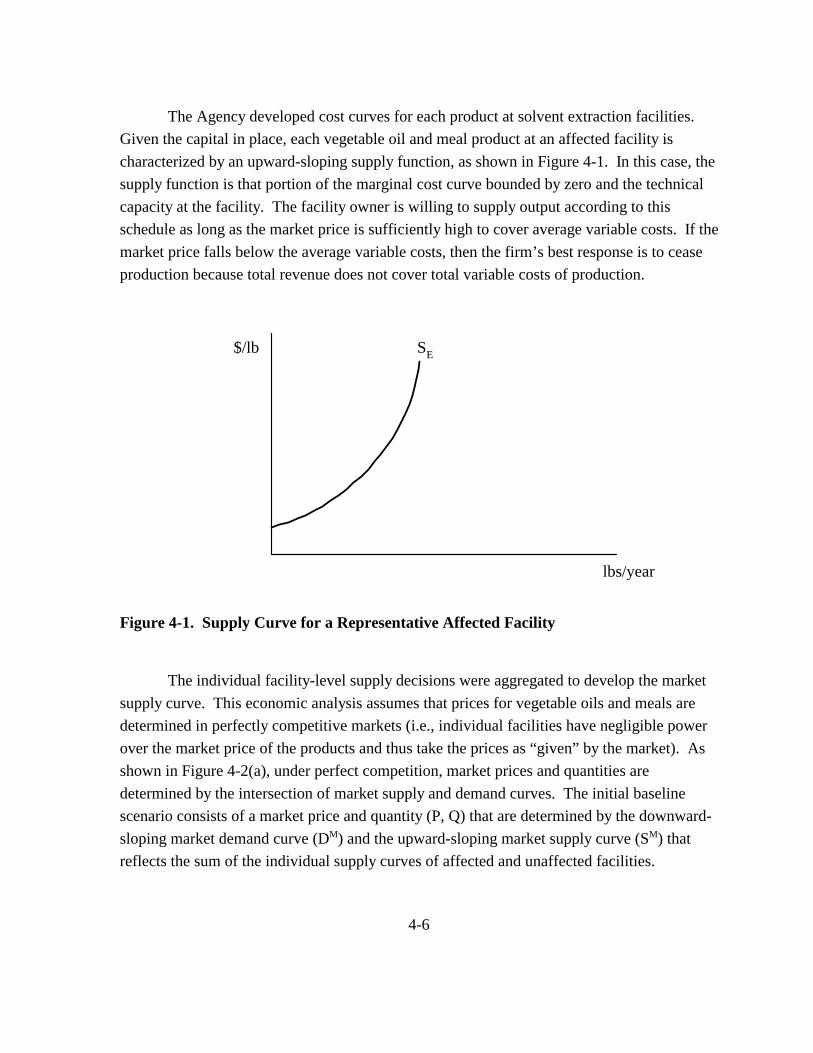
4-6

$/lb SE

lbs/year

Figure 4-1. Supply Curve for a Representative Affected Facility

The Agency developed cost curves for each product at solvent extraction facilities.

Given the capital in place, each vegetable oil and meal product at an affected facility is

characterized by an upward-sloping supply function, as shown in Figure 4-1. In this case, the

supply function is that portion of the marginal cost curve bounded by zero and the technical

capacity at the facility. The facility owner is willing to supply output according to this

schedule as long as the market price is sufficiently high to cover average variable costs. If the

market price falls below the average variable costs, then the firm’s best response is to cease

production because total revenue does not cover total variable costs of production.

The individual facility-level supply decisions were aggregated to develop the market

supply curve. This economic analysis assumes that prices for vegetable oils and meals are

determined in perfectly competitive markets (i.e., individual facilities have negligible power

over the market price of the products and thus take the prices as “given” by the market). As

shown in Figure 4-2(a), under perfect competition, market prices and quantities are

determined by the intersection of market supply and demand curves. The initial baseline

scenario consists of a market price and quantity (P, Q) that are determined by the downward-

sloping market demand curve (DM) and the upward-sloping market supply curve (SM) that

reflects the sum of the individual supply curves of affected and unaffected facilities.

4-7

P

Ss

qs qm Q

Solvent ExtractionFacilities

Sm SM

DM

P P+ =

Mechanical ExtractionFacilities

Market

a) Baseline Equilibrium

P

q′s qm Q′Solvent Extraction

Facilities

Sm SM′

DM

P P+ =

Mechanical ExtractionFacilities

Market

b) With Regulation Equilibrium

P′

Ss

qs q′m Q

SM

P′ P′

S′s

Figure 4-2. Market Equilibrium Without and With Regulation

Now consider the effect of the regulatory control costs. These costs include the

variable component consisting of the operating and maintenance costs and the nonvariable

component consisting of the compliance capital equipment required for the regulatory option.

Incorporating the regulatory control costs involves shifting upward the supply curve for each

affected facility by the per-unit compliance cost. As a result of the upward shift in the supply

4-8

curve for each affected facility, the market supply curve for each affected vegetable oil will

shift upward to reflect the increased costs of production at solvent-extraction facilities.

The estimated per-unit annual compliance cost of the MACT standard was

incorporated into the baseline market scenario as shown in Figure 4-2(b). In the baseline

scenario without the standards, at the projected price, P, the industry would produce total

output, Q, with solvent-extraction facilities producing the amount qs and mechanical

extraction facilities accounting for Q minus qs, or qm. The regulation raises the average total

cost (annual capital costs plus operating and maintenance) of solvent extraction facilities,

causing their supply curves to shift upward from Ss to Ss� and the market supply curve to shift

upward to SM�. At the new equilibrium with the regulation, the market price increases from P

to P� and market output (as determined from the market demand curve, DM) declines from Q

to Q�. This reduction in market output is the net result of reductions at solvent extraction

facilities and increases at mechanical extraction facilities.

To estimate the economic impacts of the regulation under this scenario, EPA

operationalized the conceptual model described above in a Lotus 1-2-3 multiple spreadsheet

model for each vegetable oil and meal market. Appendix A provides the details of the

operational market model for this economic analysis. In summary, this model characterizes

domestic and foreign producers and consumers of each product and their behavioral

responses to the imposition of the regulatory compliance costs. These costs are expressed per

pound of product for each facility and serve as the input to the market model, or the “cost

shifters” of the baseline supply curves at the facility. Given these costs for directly affected

facilities, the model determines a new equilibrium solution in a comparative static approach

with higher market prices and reductions in output of each product.

4.3 Economic Model Assumptions

In developing and implementing the economic model, several assumptions were

necessary. These assumptions are either numerical or operational. This section describes

each type of assumption.

4.3.1 Operational Assumptions

The operational assumptions of the model influence the structure and coverage of the

model. They are as follows:

4-9

� The domestic markets for crude vegetable oils and meals are perfectlycompetitive.

� The U.S. may potentially influence the price of crude vegetable oils and meals inthe world market (i.e., the U.S. is not a price-taker).

� Vegetable oils and meals are produced in fixed proportions relative to the oilseedinputs.

� The markets for by-products and co-products of the vegetable oil and mealproduction process will be unaffected by the regulation.

� The markets for specialty use products, which are primarily produced from crudemeals, will be unaffected by the regulation.

� The baseline year for the analysis, which is 1995, is representative of a typicalyear for the industry.

� The markets for the other vegetable oils and meals (canola, flaxseed, peanut,safflower, and sunflower) are sufficiently similar that they can be combined.

In Section 6, each of these operational assumptions is explained further. In addition,

the impact of each assumption on the results of the model is described. For example, if 1995

was a better than typical year for the industry, then the estimated percentage price effects

would appear smaller for the baseline year than in a typical year. However, based on the

estimates of the CSRs using 1999 data, as described in Section 4.1.3, the results of the model

would likely not differ substantially using more recent data.

4.3.2 Numerical Assumptions

The numerical assumptions of the economic model are the actual values used in

developing the spreadsheet model. These include the demand, supply, and trade elasticities

used in the model as well as the methods for allocating seed costs and compliance costs to the

joint oil and meal products at each facility. These assumptions are described briefly below.

4.3.2.1 Elasticity Assumptions

In determining the elasticity values to use in the economic model, the Agency

reviewed the economics literature and estimated econometric models. Appendix B describes

each paper that cites relevant elasticity estimates and presents the results of the independent

econometric estimates. The elasticities used in the model, which were obtained from both

sources, are listed in Table 4-3 (see Section B.4 for a more complete description).

4-10

In general, the demand elasticities used in the model were obtained from the

independent econometric estimates. The one exception is that the econometrically estimated

cottonseed oil demand elasticity was outside the range of the econometric estimates; thus, an

estimate from the literature was used. In the case of supply elasticities, the values used are

based on estimates in the literature for soybean products.

To investigate the impacts of alternative elasticity values on the economic model

results, EPA conducted a sensitivity analysis. The economic model was run using, in one

case, the elasticity values expected to generate the greatest effects and, in the other case, the

elasticity values expected to generate the smallest effects. These results are presented in

Table 4-3. Elasticity Estimates Used in the Economic Impact Analysis

Product Elasticity Used for the EIA

Demand Elasticities Corn oil –0.39

Cottonseed oil –0.65

Soybean oil –0.34

All other oils –0.33

Corn germ meal –0.46

Cottonseed meal –1.01

Soybean meal –0.27

All other meals –0.64

Supply Elasticities Corn oil 0.44

Cottonseed oil 0.44

Soybean oil 0.44

All other oils 0.44

Corn germ meal 0.28

Cottonseed meal 0.28

Soybean meal 0.28

All other meals 0.28

Import Supply Elasticities All products 1.00

Export Demand Elasticities All products –1.00

4-11

Appendix C. In general, the projected effects of the regulation are not particularly sensitive

to changes in the elasticity values.

4.3.2.2 Allocation of Compliance Costs to Oils and Meals

Facility-level compliance costs were allocated to oil and meal products produced at

the facility based on the relative shares of revenue generated by each product. First,

facility-level revenues were calculated for oils and for meals and then expressed as a

proportion relative to total revenue from both products. Then, facility-level compliance costs

were then allocated to each product using these proportions.

This method is preferable to allocating compliance costs based on the proportion of

the weight of the respective products relative to the weight of the oilseed input. This is

because oil generates more revenue relative to its weight than meal. (For example, soybeans

are approximately 20 percent oil and 80 percent meal by weight, but oil generates 45 percent

and meal generates 55 percent of the revenue.) Thus, this method would allocate too much of

the compliance costs to meal.

4.3.2.3 Allocation of Seed Costs to Oils and Meals

Similar to the issue with compliance costs, seed costs were allocated separately to

vegetable oils and oilseed meals to facilitate construction of supply curves for each individual

product. Seed costs were allocated to each product based on its proportion of revenue. First,

facility-level revenues were calculated at each plant using market prices for oils and meals,

and seed costs were calculated using market prices for oilseeds. The industry average

percentage of the oilseed cost relative to total revenue (averaged over oilseed types) was used

to allocate oilseed cost to each individual product. For cottonseed, the average proportion of

cottonseed cost relative to total revenue is approximately 61 percent. Thus, it was assumed

that 61 percent of the revenue generated from cottonseed oil is the cost of cottonseed used in

its production, and 61 percent of the revenue generated from cottonseed meal is the cost of

cottonseed used in its production. For soybeans, the average value is approximately

85 percent and for corn germ, the average value is approximately 77 percent. Since market

prices are missing for most of the other types of oilseeds and oilseed products, 73 percent,

which is the average of the soybean value and cottonseed value, was assumed.

4-12

4.4 Economic Impact Results

This section provides the economic impacts of the MACT regulation. The model

results are summarized below as market-, industry-, and society-level impacts due to the

regulation.

4.4.1 Market-Level Results

Table 4-4 compares 1995 baseline values with the projected effects of the two

regulatory scenarios for each of the eight vegetable oil and meal markets. Compliance costs

are ten to 12 times larger for the above-the-floor option than the MACT floor option and

therefore have much greater market-level effects. In all cases, the following changes occur:

� market price increases,

� production by domestic solvent extraction facilities decreases,

� production by domestic mechanical extraction facilities increases or remainsunchanged,

� exports decrease, and

� imports increase.

Under the floor scenario, the size of the effects in percentage change terms is similar

across all of the markets. Price increases for oils range from 0.16 percent for all other

vegetable oils to 0.48 percent for cottonseed and corn oil. Output decreases range from 0.11

percent for all other vegetable oil to 0.35 percent for cottonseed oil. In the meal markets,

price increases range from 0.10 percent for all other vegetable oils to 0.34 percent for corn

germ meal. Output decreases range from 0.07 percent for all other vegetable meals to 0.27

percent for cottonseed meal.

4.4.2 Industry-Level Results

Table 4-5 compares the 1995 baseline industry measures with the effects of the two

regulatory scenarios for the total domestic industry, domestic solvent extraction facilities, and

domestic mechanical extraction facilities. As with the market-level effects, effects are greater

for the above-the-floor option compared to the floor option. The following general changes

are projected to occur:

� industry revenues increase as a result of higher market prices that offset decreasesin output,

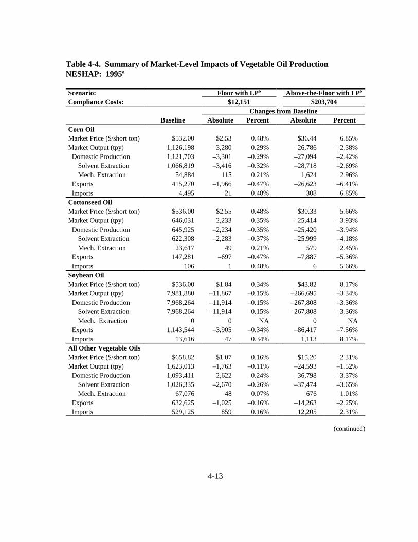
4-13

Table 4-4. Summary of Market-Level Impacts of Vegetable Oil ProductionNESHAP: 1995a

Scenario: Floor with LPb Above-the-Floor with LPb

Compliance Costs: $12,151 $203,704Changes from Baseline

Baseline Absolute Percent Absolute PercentCorn OilMarket Price ($/short ton) $532.00 $2.53 0.48% $36.44 6.85%Market Output (tpy) 1,126,198 –3,280 –0.29% –26,786 –2.38%

Domestic Production 1,121,703 –3,301 –0.29% –27,094 –2.42%Solvent Extraction 1,066,819 –3,416 –0.32% –28,718 –2.69%Mech. Extraction 54,884 115 0.21% 1,624 2.96%

Exports 415,270 –1,966 –0.47% –26,623 –6.41%Imports 4,495 21 0.48% 308 6.85%

Cottonseed OilMarket Price ($/short ton) $536.00 $2.55 0.48% $30.33 5.66%Market Output (tpy) 646,031 –2,233 –0.35% –25,414 –3.93%

Domestic Production 645,925 –2,234 –0.35% –25,420 –3.94%Solvent Extraction 622,308 –2,283 –0.37% –25,999 –4.18%Mech. Extraction 23,617 49 0.21% 579 2.45%

Exports 147,281 –697 –0.47% –7,887 –5.36%Imports 106 1 0.48% 6 5.66%

Soybean OilMarket Price ($/short ton) $536.00 $1.84 0.34% $43.82 8.17%Market Output (tpy) 7,981,880 –11,867 –0.15% –266,695 –3.34%

Domestic Production 7,968,264 –11,914 –0.15% –267,808 –3.36%Solvent Extraction 7,968,264 –11,914 –0.15% –267,808 –3.36%Mech. Extraction 0 0 NA 0 NA

Exports 1,143,544 –3,905 –0.34% –86,417 –7.56%Imports 13,616 47 0.34% 1,113 8.17%

All Other Vegetable OilsMarket Price ($/short ton) $658.82 $1.07 0.16% $15.20 2.31%Market Output (tpy) 1,623,013 –1,763 –0.11% –24,593 –1.52%

Domestic Production 1,093,411 2,622 –0.24% –36,798 –3.37%Solvent Extraction 1,026,335 –2,670 –0.26% –37,474 –3.65%Mech. Extraction 67,076 48 0.07% 676 1.01%

Exports 632,625 –1,025 –0.16% –14,263 –2.25%Imports 529,125 859 0.16% 12,205 2.31%

(continued)

4-14

Table 4-4. Summary of Market-Level Impacts of Vegetable Oil ProductionNESHAP: 1995a (Continued)

Scenario: Floor with LPb Above-the-Floor with LPb

Compliance Costs: $12,151 $203,704Changes from Baseline

Baseline Absolute Percent Absolute PercentCorn Germ MealMarket Price ($/short ton) $88.40 $0.30 0.34% $11.33 12.81%Market Output (tpy) 1,473,651 –3,304 –0.22% –84,725 –5.75%

Domestic Production 1,473,651 –3,304 –0.22% –84,725 –5.75%Solvent Extraction 1,401,546 3,373 –0.24% –87,201 –6.22%Mech. Extraction 72,105 69 2,476

Exports 61,950 –212 –0.34% –7,036 –11.36%Imports 0 0 NA 0 NA

Cottonseed MealMarket Price ($/short ton) $123.20 $0.34 0.27% $4.38 3.56%Market Output (tpy) 1,826,100 –5,019 –0.27% –63,320 –3.47%

Domestic Production 1,826,100 –5,019 –0.27% –63,320 –3.47%Solvent Extraction 1,744,562 –5,081 –0.29% –64,122 –3.68%Mech. Extraction 81,538 62 0.08% 802 0.98%

Exports 89,700 –244 –0.27% –3,082 –3.44%Imports 0 0 NA 0 NA

Soybean MealMarket Price ($/short ton) $173.80 $0.47 0.27% $12.49 7.19%Market Output (tpy) 31,290,977 –35,793 –0.11% –892,586 –2.85%

Domestic Production 31,225,572 –35,970 –0.12% –897,287 –2.87%Solvent Extraction 31,225,572 –35,970 –0.12% –897,287 –2.87%

Mechanical Extraction 0 0 NA 0 NAExports 6,491,570 –17,571 –0.27% –435,309 –6.71%Imports 65,405 178 0.27% 4,701 7.19%

All Other Vegetable OilMealsMarket Price ($/short ton) $93.22 $0.10 0.10% $1.86 1.99%Market Output (tpy) 2,520,129 –1,729 –0.07% –32,548 –1.29%

Domestic Production 1,583,559 –2,704 –0.17% –51,186 –3.23%Solvent Extraction 1,497,886 –2,729 –0.18% –51,660 –3.45%Mechanical Extraction 85,673 25 0.03% 474 0.55%

Exports 138,469 –144 –0.10% –2,702 –1.95%Imports 936,570 975 0.10% 18,638 1.99%

a Facilities that began operation in 1996 or later years are not included in the analysis.b LP represents lost production costs that may be incurred due to the downtime to install new capital

equipment. NA = not available.

4-15

Table 4-5. Summary of Industry-Level Impacts of Vegetable Oil ProductionNESHAP: 1995a

Floor with LPb Above-the-Floor with LPb

Changes from BaselineBaseline Absolute Percent Absolute Percent

Total IndustryRevenues ($103) $11,963,996 $17,728 0.1% $447,584 3.7%

Costs ($103) $10,567,809 –$6,394 –0.1% –$216,276 –2.0%

Post-regulatory $0 $12,076 NA $163,977 NA

Oil and Meal Production $10,567,809 –$18,470 –0.2% –$380,253 –3.6%

Gross Profits ($103) $1,396,186 $24,122 1.7% $663,860 47.5%

Operating Entities

Product-Line Closures NA 0 NA 6 NA

Facility Closures NA 0 NA 3 NA

Employment Loss NA –12 NA –350 NA

Solvent ExtractionRevenues ($103) $11,853,542 $17,264 0.1% $440,414 3.7%

Costs ($103) $10,482,567 –$6,477 –0.1% –$217,808 –2.1%


Production $10,482,567 –$18,554 –0.2% –$381,785 –3.6%

Gross Profits ($103) $1,370,975 $23,741 1.7% $658,222 48.0%

Operating Entities

Product Lines 111 0 0.0% 6 5.4%

Facilities 106 0 0.0% 3 2.8%

Employment 5,673 –12 –0.2% –350 –6.2%

Mechanical ExtractionRevenues ($103) $110,454 $464 0.4% $7,170 6.5%

Costs ($103) $85,242 $84 0.1% $1,532 1.8%

Post-regulatory $0 $0 0.0% $0 0.0%

Production $85,242 $84 0.1% $1,532 1.8%

Gross Profits ($103) $25,212 $380 1.5% $5,638 22.4%

Operating Entities

Product Lines NA NA NA NA NA

Facilities NA NA NA NA NA

Employment NA NA NA NA NA


equipment.NA = not available.

4-16

� net industry costs decrease,

� production costs decrease for solvent extraction facilities due to decreasedproduction levels,

� production costs increase for mechanical extraction facilities due to increasedproduction levels,

� gross industry profits increase (revenue less direct costs of production andcompliance costs), and

� industry employment decreases due to decreased production levels and/or lineclosures.

No product-line or facility closures are predicted with the floor option, including lost

production costs. Six product-line closures and three facility closures are predicted with the

above-the-floor option. However, it should be noted that the estimates of facility and

product-line closures are sensitive to the accuracy of the baseline characterization of facilities

and the estimation of their costs to comply with the NESHAP.

Although total gross profits for solvent extraction facilities are projected to increase

1.7 percent under the floor option, some facilities are projected to experience decreased gross

profits. Facilities with profit losses are those with higher than average variable production

costs (labor, energy, and materials) and/or compliance costs relative to the facilities with

profit gains. Facilities with profit gains benefit from increased market price and the ability to

pass some of the regulatory costs on to consumers.

Table 4-6 separates the number of facilities projected to experience profit losses from

those projected to experience profit gains. The factors differentiating facilities with profit

losses and those with profit gains are as follows:

� profit losers have smaller capacity facilities (one-third of the size of profitgainers),

� profit losers have greater solvent loss ratios per ton of oilseed (two to four times greater than profit gainers), and

� profit losers have greater compliance costs per ton of oilseed (four times greater

than profit gainers).

4.4.3 Social Costs of the Regulation

The social costs of a regulation are traditionally measured as changes in both

consumer and producer economic welfare (see Appendix A for a more complete discussion).

4-17

Table 4-6. Summary of Distributional Industry Impacts of Vegetable Oil ProductionNESHAP: 1995a


Solvent Extraction Facilities

WithProfit Loss

With ProfitGain Total

WithProfit Loss

With ProfitGain Total

Number

Facility Capacity (tpd) 21 85 106 22 84 106

Total 11,362 161,841 173,203 13,610 159,593 173,203

Average Per Facility 541 1,904 1,634 619 1,900 1,634

Annual Solvent Loss

Total (103 gallons) 2,419 13,577 15,996 2,682 13,314 15,996

Gallons per Ton of Oilseed 0.84 0.28 0.31 0.84 0.28 0.31

Incremental Compliance Costs

Total ($103/yr) $2,502 $9,649 $12,151 $54,191 $149,513 $203,704

Per ton of oilseed $0.87 $0.20 $0.24 $16.93 $3.14 $4.01

Change in Gross Profits ($103/yr)c –$1,184 $24,925 $23,741 –$16,885 $675,106 $658,222

Change in Employment (FTEs)d –7 –5 –12 –213 –137 –350


equipment.c Gross profits calculated as revenue less costs of production including oilseed costs.d FTEs = Full-time equivalents.

The vegetable oil NESHAP directly affects consumers and producers of vegetable oils and

meals. Consumers experience reductions in economic welfare (i.e., consumer surplus) due to

increased market prices and decreased market quantity. Producers may experience either

increases or decreases in economic welfare (i.e., producer surplus) as a result of increased

market prices, decreased costs of production, and imposition of the compliance costs.

Table 4-7 compares the welfare effects of the NESHAP on domestic consumers,

domestic producers, and foreign producers. Consumer surplus decreases in all eight

4-18

Table 4-7. Distribution of the Social Costs Associated with the Vegetable OilProduction NESHAP: 1995a


Social Cost Component Change in Value ($103)

Consumer Surplus –$36,929 –$842,168

Corn Oil –$2,845 –$40,554

Cottonseed Oil –$1,644 –$19,207

Soybean Oil –$14,649 –$343,893

All Other Vegetable Oils –$1,734 –$24,470

Corn Germ Feed –$446 –$16,212

Cottonseed Meal –$613 –$7,865

Soybean Meal –$14,752 –$385,322

All Other Vegetable Meals –$244 –$4,645

Producer Surplus $24,846 $675,388

Domestic Producers $24,122 $663,860

Solvent Extraction $23,741 $658,222

Mechanical Extraction $380 $5,638

Foreign Producers $725 $11,528

Social Costs of Regulation –$12,083 –$166,780


equipment.

vegetable oil and meal markets under both regulatory scenarios. Consumer surplus losses

range from $36.9 million for the floor option to $842.2 million for the above-the-floor option

including lost production costs. Domestic producer surplus increases under both regulatory

scenarios, although, as noted in Section 4.4.2, some producers gain while others lose.

Foreign producer surplus increases as a result of higher prices and increased imports. In

total, the social costs of the regulation range from $12.1 million to $166.8 million.

1Company-level sales figures used for this analysis were obtained from publicly available sources.

5-1

SECTION 5

SMALL BUSINESS IMPACTS

This regulatory action will potentially affect owners of vegetable oil and meal

processing facilities. Firms or individuals that own these facilities are legal business entities

that have the capacity to conduct business transactions and make business decisions that

affect the facility. The legal and financial responsibility for compliance with a regulatory

action ultimately rests with these owners who must bear the financial consequences of their

decisions. Environmental regulations like this rule affect all businesses, large and small, but

small businesses may have special problems in complying with such regulations.

The RFA of 1980 requires that special consideration be given to small entities

affected by federal regulation. The RFA was amended in 1996 by SBREFA to strengthen the

RFA’s analytical and procedural requirements.

This section identifies the small businesses that will be affected by this NESHAP and

provides a screening-level analysis to assist in determining whether this rule imposes a

significant impact on a substantial number of small businesses. The screening-level analysis

described in this section is a “sales test,” which computes the annualized compliance costs as

a percentage of sales for each company.1 In addition, this section provides information about

the likely impact on small businesses after accounting for producer responses to the

regulation and resulting changes in market prices and output for vegetable oils and meals.

Information on cottonseed facilities is provided separately because they make up a

disproportionate number of the facilities owned by small companies.

The SBA defines a small business involved in vegetable oil and meal processing as

follows:

� Corn Oil (NAICS 311221)—fewer than 750 total employees;

� Corn Oil Dry Milling (NAICS 311211)—fewer than 500 total employees;

5-2

� Cottonseed Oil (NAICS 311223)—fewer than 1,000 total employees;

� Soybean Oil (NAICS 311222)—fewer than 500 total employees; and

� All Other Vegetable Oils (NAICS 311223)—fewer than 1,000 total employees.

Based on these definitions, 15 companies, which are listed in Table 5-1, can be classified as

small or potentially small businesses. Two firms without available employment data are

included as potentially small businesses. As of 1995, these 15 companies owned and

operated 21 facilities, or 20 percent of all solvent extraction facilities.

For the purposes of assessing the impact of this rule on these small businesses, the

Agency calculated the share of annual compliance cost relative to baseline sales for each

company. For this screening-level analysis, annual compliance costs were defined as the

engineering control costs imposed on these companies; thus, they do not reflect the changes

in production expected to occur in response to imposition of these costs and the resulting

market adjustments. Table 5-2 compares total compliance costs for small and large

companies for each of the two scenarios. Small companies own 20 percent of the facilities

and incur compliance costs of $2.2 million (18 percent) under the floor with lost production

costs scenario and $21.1 million (10 percent) under the above-the-floor with lost production

costs scenario.

Mean, minimum, and maximum CSRs under each scenario are presented in

Table 5-3. Mean CSRs for all companies are 0.16 percent under the floor with lost

production costs scenario and 1.62 percent under the above-the-floor with lost production

costs scenario. Under the floor scenario, the mean CSR for small companies is 0.30 percent,

ranging from a low of 0.03 to 0.61 percent, while the mean ratio is 0.04 percent for large

companies. Under the above-the-floor scenario, the mean CSR for small companies is

2.97 percent, and the mean CSR for large companies is 0.45 percent. Table 5-4 presents the

distribution of CSRs for small, large, and all companies combined for each of the scenarios.

All large and small companies have CSRs less than 1 percent under the floor scenario. Under

the above-the-floor scenario, 13 small companies and three large companies have CSRs

above 1 percent.

5-3

Table 5-1. Summary Data for Small Companies: 1995

Company NameNumber of

Affected FacilitiesSales

($ million)Total

Employment Year ReportedChickasha Cotton Oil Company 4 $93.0 600 1995Delta Oil Mill 1 $22.5 90 1996Hartsville Oil Mill Incorporated 1 $20.0 100 1996J.G. Boswell 1 $80.0 1,000 1993Oilseeds International 1 NA NA NAOsceola Products 2 $50.0 170 1996Owensboro Grain Company 1 $450.0 195 1996Plains Cooperative Oil Mill, Inc. 1 $128.0 108 1995Planter’s Cotton Oil Mill 1 $35.0 100 1996Producers Cooperative Mill 1 $35.0 100 1996Rito Partnershipa 1 NA NA NASessions Company 1 $30.0 100 1994Southern Soya Corporation 1 NA 89 1996Valley Cooperative Mills 1 $32.0 100 1992Yazoo Valley Oil Mill, Inc. 3 $113.7 300 1996TOTAL 21 NA NA NA

NA = Not available.

a Rito Partnership operates a rice oil facility that will not be subject to the regulation. It is included in the aggregate totals to maintainconfidentiality in the tables that present production data.

Note: The Small Business Administration (SBA) defines a small business for industries affected by this regulation as follows:Corn Oil (NAICS 311221) = fewer than 750 total employeesCorn Oil Dry Milling (NAICS 311211) = fewer than 500 total employeesCottonseed Oil (NAICS 311223) = fewer than 1,000 total employeesSoybean Oil (NAICS 311222) = fewer than 500 total employeesAll Other Vegetable Oils (NAICS 311223) = fewer than 1,000 total employees

Sources: Information Access Corporation. 1997 Business Index [computer file]. Foster City, CA: Information Access Corporation.The Dialog Corporation. 1997. Dun & Bradstreet Market Identifiers [computer file]. New York, NY: Dun & Bradstreet. <http://www.profound.com>.

5-4

Table 5-2. Capacity and Compliance Cost Comparisons for Small and Large Companies: 1995

Capacity (tons per day) Compliance Costs ($103)

Company Size

Number of Companies

Number of Facilities

Share of Facilities Total Share

Floor with LPa

Above-the-Floor with LP

Small 15 21 19.8% NR NR $2,153 $21,089

Large 16 85 80.2% NR NR $9,998 $182,615

TOTAL 31 106 100.00% 172,803 100.00% $12,151 $203,704

NR = Not reported to avoid disclosure of CBI.

a LP represents lost production costs that may be incurred due to the downtime to install new capital equipment.

5-5

Table 5-3. Summary of Cost-to-Sales Ratios for the Vegetable Oil NESHAP: 1995 (%)

Scenario

Floor with LPa Above-the-Floor with LP

Company Size Mean Min Max Mean Min Max

Small 0.30 0.03 0.61 2.97 0.51 6.11

Large 0.04 <0.01 0.11 0.45 <0.01 1.30

TOTAL 0.16 <0.01 0.61 1.62 <0.01 6.11


5-6

Table 5-4. Distribution of Cost-to-Sales Ratios for the Vegetable Oil NESHAP: 1995

Scenario

Floor with LPa Above-the-Floor with LP

Number Share Number Share

Small Companies

0-1% 15 100.0% 2 13.3%

1-2% 0 0.0% 2 13.3%

>2% 0 0.0% 11 73.3%

TOTAL 15 100.0% 15 100.0%

Large Companies

0-1% 16 100.0% 13 81.3%

1-2% 0 0.0% 3 18.8%

>2% 0 0.0% 0 0.0%

TOTAL 16 100.0% 16 100.0%

All Companies

0-1% 31 100.0% 15 48.4%

1-2% 0 0.0% 5 16.1%

>2% 0 0.0% 11 35.5%

TOTAL 31 100.0% 31 100.0%


2In 1995, 25 cottonseed facilities were operating. Since then, ten of these facilities have closed. Closures havebeen particularly high in this industry because cottonseed is being used increasingly as a dairy feed. Thevalue of cottonseed as a feed product has risen relative to its value in producing oil and meal products(Wedegaertner, 1999). Hence, cottonseed oil and meal processing has become less profitable.

5-7

Because small businesses affected by this regulation own many cottonseed processing

facilities and several of these facilities have closed since the baseline year of analysis,2 the

Agency undertook additional analysis to determine whether companies that operate these

facilities will experience significant economic impacts as a result of the regulation. CSRs

were calculated both for the plants included in the 1995 baseline and then for currently

operating plants using publicly available sales data. Under the floor with lost production

costs scenario, the average CSR for small companies that owned cottonseed processing

facilities in 1995 falls below 1 percent (0.31 percent) with a maximum value of 0.59 percent

(see Tables 5-5 and 5-6). None of these companies have CSRs above 1 percent. However,

under the above-the-floor with lost production costs scenario, the average CSR in 1995 is 2.9

percent with a maximum value of 4.3 percent. All ten companies have CSRs above 1

percent, eight of which are greater than 2 percent. Although ten cottonseed facilities have

closed since 1995, excluding the compliance costs for facilities not currently operating does

not significantly alter the analysis. The one exception is that two companies no longer

operate any cottonseed facilities and therefore are not affected under the above-the-floor

scenario.

CSRs for companies that own cottonseed facilities were also calculated using facility

revenues as the denominator rather than publicly available company sales data. These facility

CSRs exclude revenues that companies may generate from operations other than vegetable oil

production. In this case, for the nine cottonseed processing facilities operating in 1995 and

still currently operating that are owned by small businesses, the average facility-level CSR is

0.28 percent and ranges from 0.05 percent to 0.52 percent (see Table 5-7). Thus, the results

are not substantially different using facility-level revenues instead of company sales. In

addition, the facility CSRs for compliance cost data cottonseed facilities were recomputed

using 1999 price data and projected to 1999 using the producer price index. The purpose of

this analysis was to determine whether cottonseed facility CSRs would change substantially

using more recent data. For the cottonseed processing facilities operating in 1995 and still

operating currently that are owned by small businesses, the average facility-level CSR

increased to only 0.33 percent with a range from 0.06 percent to 0.58 percent.

5-8

Table 5-5. Summary of Company Cost-to-Sales Ratios for Companies That Own Cottonseed Facilities: 1995 (%)

Operating 1995a Currently Operatingb

Floor with LPc Above-the-Floor with LP Floor with LP Above-the-Floor with LP

Company Size Mean Min Max Mean Min Max Mean Min Max Mean Min Max

Small 0.31 0.03 0.59 2.91 1.01 4.32 0.22 0.03 0.51 2.35 0.86 4.32

Large 0.02 0.02 0.02 0.37 0.23 0.50 0.01 <0.01 0.02 0.24 <0.01 0.47

TOTAL 0.26 0.02 0.59 2.49 0.23 4.32 0.18 <0.01 0.51 1.96 <0.01 4.32

a Companies with cottonseed facilities operating in 1995.b Companies with cottonseed facilities currently operating.c LP represents lost production costs that may be incurred due to the downtime to install new capital equipment.

5-9

Table 5-6. Distribution of Cost-to-Sales Ratios for Companies That Own Cottonseed Facilities: 1995


Floor with LPc Above-the-Floor with LP Floor with LP Above-the-Floor with LP

Number Share Number Share Number Share Number Share

Small Companies

0-1% 10 100.0% 0 0.0% 9 100.0% 1 11.1%

1-2% 0 0.0% 2 20.0% 0 0.0% 3 33.3%

>2% 0 0.0% 8 80.0% 0 0.0% 5 55.6%

TOTAL 10 100.0% 10 100.0% 9 100.0% 9 100.0%

Large Companies

0-1% 2 100.0% 2 100.0% 2 100.0% 1 100.0%

1-2% 0 0.0% 0 0.0% 0 0.0% 0 0.0%

>2% 0 0.0% 0 0.0% 0 0.0% 0 0.0%

TOTAL 2 100.0% 2 100.0% 2 100.0% 1 100.0%

All Companies

0-1% 12 100.0% 2 16.7% 11 100.0% 2 27.3%

1-2% 0 0.0% 2 16.7% 0 0.0% 3 27.3%

>2% 0 0.0% 8 66.7% 0 0.0% 5 45.5%

TOTAL 12 100.0% 12 100.0% 11 100.0% 10 100.0%

a Companies with cottonseed facilities operating in 1995.b Companies with cottonseed facilities currently operating.c LP represents lost production costs that may be incurred due to the downtime to install new capital equipment.

5-10

Table 5-7. Summary of Facility Cost-to-Sales Ratios for Cottonseed Facilities: 1995 (%)


Floor with LPc

Company Size Mean Minimum Maximum Mean Minimum Maximum

Small 0.54 0.05 1.57 0.28 0.05 0.52

Large 0.25 0.07 0.64 0.20 0.07 0.52

TOTAL 0.43 0.05 1.57 0.25 0.05 0.52

a Facilities operating in 1995.b Facilities currently operating.c LP represents lost production costs that may be incurred due to the downtime to install new capital equipment.

5-11

In summary, the Agency’s screening analysis does not suggest a significant negative

impact on a substantial number of small companies under the MACT floor alternative

promulgated by the EPA (this scenario includes lost production costs). The economic

impacts model verifies that the effects of taking into account market adjustments are small.

However, the potential for negative impacts is greater under the above-the-floor scenario.

Table 5-8 summarizes the economic impacts of the regulation on small companies.

Gross profits are projected to increase by 0.2 percent for small companies under the floor

with lost production costs scenario. The projected effects of the above-the-floor with lost

production costs scenario are greater than the floor scenario, but no closures are expected

under either of the scenarios.

5-12

Table 5-8. Summary of Small Business Impacts of Vegetable Oil Production NESHAP: 1995

Floor with LPa Above-the-Floor with LPa

Changes From Baseline

Baseline Absolute Percent Absolute Percent

Revenues ($103) $780,636 –$793 –0.1% $13,629 1.7%

Costs ($103) $665,767 –$1,010 –0.2% –$7,777 –1.2%


Production $665,767 –$3,141 –0.5% –$27,363 –4.1%

Gross Profits ($103) $114,869 $217 0.2% $21,405 18.6%

Operating Entities

Product Lines 21 0 0.0% 0 0.0%

Facilities 20 0 0.0% 0 0.0%

Employment NR –6 NR –59 NR

NA = Not available.NR = Not reported to avoid disclosure of CBI.


6-1

SECTION 6

ASSUMPTIONS AND LIMITATIONS OF THE ECONOMIC MODEL

In developing the economic model of the vegetable oil and meal markets, several

assumptions were necessary to make the model operational. These assumptions are in

addition to the numerical assumptions described in Section 4.3.2 (i.e., elasticity values and

allocation of both seed costs and compliance costs to individual products). In this section,

each operational assumption is listed and explained. Possible impacts and limitations of the

model resulting from each assumption are then described.

Assumption: The domestic markets for crude vegetable oils and meals are perfectlycompetitive.

Explanation: Assuming that the markets for crude vegetable oils and meals are perfectly

competitive implies that individual producers cannot individually affect the prices they

receive for their products. The measures available to determine whether a market is perfectly

competitive are the four-firm concentration ratios (CR4) and the Herfindahl-Hirschman

indexes (HHIs). The most recently available measures are based on SIC code-level data for

1992. Based on the 1992 data, the CR4s for vegetable oils range from a low of 62 percent for

SIC 2074 (Cottonseed Oil Mills) to a high of 89 percent for SIC 2076 (Vegetable Oil Mills,

Except Corn, Soybean, and Cottonseed). Similarly, the HHIs range from a low of 1,430 for

SIC 2074 to a high of 2,119 for SIC 2076. These concentration measures considered in

isolation imply that the vegetable oil industry is moderately imperfectly competitive.

However, given the homogeneous nature of crude vegetable oils and meals and that there

appear to be large economies of scale in their production, the assumption of perfect

competition is appropriate.

Possible impact: If the markets for crude vegetable oils and meals were in fact imperfectly

competitive, implying that individual producers can exercise market power and thus affect

the prices they receive for their products, the economic model would understate possible

price increases due to the regulation and the social costs of the regulation. Under imperfect

competition, producers would be able to pass along more of the costs of the regulation to

consumers; thus, consumer surplus losses would be greater.

6-2

Assumption: The U.S. is not a price-taker on the world market for crude vegetable oilsand meals; that is, the U.S. may influence the price of these products on the worldmarket.

Explanation: Assuming that the U.S. is not a price-taker on the world market for these

products implies that the U.S. is “large” relative to the rest of the world. That is, the U.S.

ships a sufficient quantity of these products that changes in the volume of products imported

or exported may affect prices in the world market. Thus, producers in the U.S. have the

opportunity to pass along some portion of the costs of the regulation to the consumers of

crude vegetable oils and meals (i.e., to the facilities that further process the product for

consumption by humans or animals).

Possible impact: If the U.S. was instead a price-taker on the world market for crude

vegetable oils and meals, producers in the U.S. would not be able to pass along the costs of

the regulation to consumers of these products. If U.S. companies that export crude vegetable

oils and meals attempted to raise prices as a result of the regulation, importing countries

would instead purchase from countries other than the U.S. Likewise, U.S. companies would

be unable to raise prices of these products domestically because consumers of crude

vegetable oils and meals would instead import all these products at the lower world price.

Thus, U.S. producers would have to fully absorb the costs of the regulation, and consumers

would bear none of the costs of the regulation. The potential impact under this scenario on

individual producers is estimated by the CSRs that are documented in Section 4.

Assumption: Crude vegetable oils and meals are produced in fixed proportions relativeto the oilseed inputs.

Explanation: Assuming that crude vegetable oils and meals are produced in fixed

proportions implies that facilities cannot alter the ratio of oil to meal from a given oilseed in

response to the regulation. This assumption is appropriate in light of our calculations using

production data from the USDA and information provided by the trade associations (see

Section 2.1).

Possible impact: If, in fact, facilities could alter the proportion of oil to meal, then facilities

could potentially alter the proportion in response to the regulation and thus could alleviate

some of the burden of the regulation. In particular, a facility may choose to produce more of

the product that generates higher revenues by weight (i.e., oil). However, it appears

technically infeasible for facilities to alter the proportion.

6-3

Assumption: The markets for by-products and co-products of the vegetable oil andmeal production process will be unaffected by the regulation.

Explanation: Products such as cottonseed linters, hulls, and lecithin are produced either as

by-products or co-products of the production process for vegetable oils and meals. These

markets could be potentially affected by the regulation if the regulation changes the

throughput of oilseeds in the production process. They are not modeled in this analysis

because there is insufficient data to characterize their markets (e.g., prices and output at each

facility), and they generate a relatively smaller share of revenue compared to oils and meals.

Possible impact: Because the prices and output of by-products and co-products are assumed

unchanged as a result of the regulation, the analysis may either understate or overstate

changes to revenue and costs for individual facilities. It is expected that the net effects of

these potential revenue and cost changes on individual facilities are minimal and would not

significantly alter the primary conclusions of the EIA.

Assumption: The markets for specialty use products, which are produced primarilyfrom crude meal, will be unaffected by the regulation.

Explanation: Specialty use products that are produced by vegetable oil mills include

products such as soy protein, tofu, and infant formula ingredients. The production processes

for these products are proprietary to the plant producing them, and only a handful of plants

produce each of these products. Thus, data to characterize these markets are unavailable.

Possible impact: These specialty use products generate higher revenues than crude meal;

thus, revenues are understated in the model for the plants that produce them. Therefore, the

impacts of the regulation on these plants appear larger than they may be in actuality.

Assumption: The baseline year of the analysis, which is 1995, is representative of atypical year for the industry.

Explanation: The engineering costs of the regulation are estimated for all facilities that

produced crude vegetable oils and meals in 1995. In order for the economic model to be

consistent, all costs, prices, and quantities must be denominated in the same year. In

addition, for consistency between market-level data and facility-level data, both must be

representative of the same year.

Possible impact: If 1995 was a good year relative to typical conditions (i.e., with high output

prices and low input prices), then the impacts of the regulation would appear to be smaller (in

6-4

percentage terms) than they would be for a typical year. As discussed in Section 2, the

markets for vegetable oils and meals and for the oilseeds used in their production exhibit a

great deal of volatility over time. Based on price data for the 1990s, 1995 appears to have

been a relatively good year for vegetable oil producers. To evaluate whether the results of the

economic model would differ substantially using more recent data, facility-level CSRs were

calculated using 1999 data. Based on these calculations, the CSRs increased by less than 0.1

percent except for one facility. Thus, it appears that the results of a model using 1999 data

would not differ substantially from the results using 1995 data. It is likely that the projected

percentage changes in the economic variables would increase slightly, but the overall

economic effects of the MACT floor scenario would still be small. According to a recent

USDA publication, the economic conditions of the vegetable oil and meal industries have

improved in 2000 (USDA, 2000).

Assumption: The markets for specialty oils and meals, which include canola, flaxseed,peanut, safflower, and sunflower, are sufficiently substitutable that they can beconsidered in the same market.

Explanation: Because relatively few facilities produce each of the specialty oils and meals,

and because these products are grouped in the NAICS definitions, they are considered to be

in a single market in the economic analysis. The price in the model for the oilseed input and

the oil and meal outputs are computed as weighted averages of the prices of the individual

products. By grouping these products into a single market, it is assumed that these products

are highly substitutable for one another.

Possible impact: The impacts of the regulation on speciality oils and meals may be

potentially understated or overstated because they are grouped in the analysis. However, the

impacts on each as projected by the economic model are small. There are only a handful of

producers of each of these products, and data on prices of some of the products are not

available; thus, it is not possible to model each market separately.

R-1

REFERENCES

1997 Directory of Corporate Affiliations. 1997. Vol. 5: International Public and Private

Companies. New Providence, RI: National Register Publishing.

Agriculture and Agri-Food Canada. September 1998. “An Evaluation of Oilseed Trade

Liberalization.” <http://aceis.agr.ca/policy/epad/en...pubs/wp-tp/

tms/98034tp/toc/toc.htm>.

Ailor, David C., National Oilseed Processors Association, to Linda Chappell, U.S.

Environmental Protection Agency. May 5, 1998. “NOPA Responses on EPA’s

March 1998 Draft ‘Vegetable Oil Production: Industry Profile and

Initial/Supplemental to Questions on the Industry’.”

Ailor, David C., National Oilseed Processors Association. July 25, 2000. “Comments of the

Vegetable Oil MACT Coalition on the National Emission Standards for Hazardous

Air Pollutants: Solvent Extraction for Vegetable Oil Production, 40 C.F.R. Part 63

Subpart GGGG, Air Docket No. A-97-59.” Memorandum.

Baumel, C.P. 1996. “Expanded Soybean Processing Capacity Could Impact Margins.”

Feedstuffs 68(May 20):37-41.

Brenner, Kyd, Corn Refiners Association, Inc. E-mail to Mary Muth, Research Triangle

Institute. March 15, 1999.

Chern, Wen S., Edna T. Loehman, and Steven T. Yen. 1995. “Information, Health Risk

Beliefs, and the Demand for Fats and Oils.” The Review of Economics and Statistics

77(3):555-64.

Dun & Bradstreet. 1998. Dun & Bradstreet Market Identifiers [computer file]. New York,

NY: Dialog Corporation.

Durham, J.F. June 12, 1998. “Vegetable Oil MACT—Notes for 6/16/98 Teleconference.”

Delivered to participants of the Vegetable Oil MACT teleconference.

R-2

Hoover’s Incorporated. 1998. Hoover’s Company Profiles. Austin, TX: Hoover’s

Incorporated. <http://www.hoovers.com/>.

Huang, K.S. 1993. U.S. Demand for Food: A Complete System of Price and Income Effects.

U.S. Department of Agriculture, Economic Research Service. Bulletin 1821.

Washington, DC.

Information Access Corporation. 1997. Business Index [computer file]. Foster City, CA:

Information Access Corporation.

Lence, S.H., D.J. Hayes, and W.H. Meyers. 1995. “The Behavior of Forward-Looking Firms

in the Very Short Run.” American Journal of Agricultural Economics

77(November):922-934.

Marine, C. Lockwood, Marine Associates. Facsimile to Mary Muth, Research Triangle


Meyers, W.H., P. Westhoff, D.L. Stephens, B.L. Buhr, M.D. Helmar, and K.J. Stephens.

January 1993. “FAPRI U.S. Agricultural Sector Elasticities Volume I: Crops.”

Center for Agricultural and Rural Development, Iowa State University, Ames, Iowa.

Technical Report 92-TR 25.

Midwest Research Institute. November 1995. “Emission Factor Documentation for AP-42,

Section 9.11.1. Vegetable Oil Processing.” Prepared for the U.S. Environmental

Protection Agency, Office of Air Quality Planning and Standards, Emission Factor

and Inventory Group. Cary, NC: Midwest Research Institute.

Mitsubishi Corporation. Annual Report 1996. <http://www.mitsubishi.co.jp/en/

investor/gr.html>.

National Cotton Council of America. July 25, 2000. “Comments of the National Cotton

Council and National Cottonseed Products Association on the Proposed National

Emission Standards for Hazardous Air Pollutants: Solvent Extraction for Vegetable

Oil Production (65 FR 34252; May 26, 2000) (Air Docket No. A-97-59).

Memorandum.

Standard and Poor’s Corporations [computer file]. Palo Alto, CA: Dialog Information

Service.

R-3

Ugarte, D., University of TN at Knoxville. Telecon with Mary Muth, Research Triangle


U.S. Bureau of Census. 1998a. U.S. Exports History: Historical Summary 1993-1997 on

CD-ROM [machine readable data file]. Washington: Bureau of the Census.

U.S. Bureau of Census. 1998b. U.S. Imports History: Historical Summary 1993-1997 on

CD-ROM [machine readable data file]. Washington, DC: Bureau of the Census.

U.S. Department of Agriculture. 1992. Agricultural Statistics 1992. Washington, DC:

Government Printing Office.

U.S. Department of Agriculture. 1997a. Agricultural Statistics 1997. Washington, DC:


U.S. Department of Agriculture. 1997b. Agricultural Prices: 1996 Summary. Washington,

DC: Government Printing Office.

U.S. Department of Agriculture. 1997c. Oil Crops Situation and Outlook Yearbook.

Washington, DC: Government Printing Office.

U.S. Department of Agriculture, Economic Research Service. 1997. Feed Yearbook.

[computer file]. Last updated April 1997.

U.S. Department of Agriculture, Economic Research Service. Oil Crops Outlook.

November 13, 1996.

U.S. Department of Agriculture, Economic Research Service. Oil Crops Outlook. March 13,

1996.

U.S. Department of Agriculture, Economic Research Service. Oil Crops Outlook. October

14, 1997.

U.S. Department of Agriculture, Economic Research Service. 1998. Oil Crops Yearbook.

[computer file]. Last updated January 1998.


November 12, 1998.

U.S. Department of Agriculture, Economic Research Service. Rice Yearbook. [computer

file]. Last updated November 1998.

R-4

U.S. Department of Agriculture, Economic Research Service. Sugar and Sweetener

Yearbook. [computer file]. Last updated January 1998.


September 13, 1999a.

U.S. Department of Agriculture, Economic Research Service. 1999b. Oil Crops Yearbook.

[computer file]. Last updated November 1999.

U.S. Department of Agriculture, Economic Research Service. October 1999c. “Oil Crops

Yearbook—Summary.” ERS-OCS-1099.

U.S. Department of Agriculture. 2000. Agricultural Statistics 2000. Washington, DC:


U.S. Department of Agriculture, Economic Research Service. 2000. Oil Crops Outlook.

September 13, 2000.

U.S. Department of Agriculture, Economic Research Service. 2000. Feed Yearbook.

[computer file]. Last updated May 2000.

U.S. Department of Agriculture, National Agriculture Statistics Service. 2000. Agricultural

Prices: 1999 Summary. Washington, DC: Government Printing Office.

U.S. Department of Commerce, Bureau of the Census. National Monthly Population

Estimates: 1980-2000. <http://www.census gov/population/www/

estimates/nation1.htm>. Last updated November 2, 2000.

U.S. Department of Commerce, Bureau of the Census. 1995. 1992 Census of Manufactures,

Industry Series—Fats and Oils. MC92-1-20D. Washington, DC: Government

Printing Office.

U.S. Department of Commerce, Bureau of the Census. 1995. 1992 Census of Manufactures,

Industry Series—Grain Mill Products. MC92-1-20D. Washington, DC:


U.S. Department of Commerce. 1996a. 1995 Current Industrial Reports—Fats and Oils:

Oilseed Crushings. M20J. Washington, DC: Government Printing Office.

R-5

U.S. Department of Commerce. 1996b. 1995 Current Industrial Reports—Fats and Oilseed

Crushings, Production, Consumption, and Stocks. M20K. Washington, DC:


U.S. Department of Energy, Energy Information Administration. State Energy Price and

Expenditure Report 1994 [computer file].

<http://www.eia.doe.gov/emev/sep/states.html>. Last modified June 25, 1997.

U.S. Department of Labor, Bureau of Labor Statistics. BLS LABSTAT database.

<http://www.bls.gov>. Data extracted on March 3, April 15, and April 22, 1998.

Wedegaertner, T., Cotton, Inc. Telecon with Mary Muth, Research Triangle Institute.

August 17, 1999.

Yen, S.T., and W.S. Chern. 1992. “Flexible Demand Systems with Serially

Correlated Errors: Fat and Oil Consumption in the United

States.” American Journal of Agricultural Economics 74(3):689-697.

Zukor, C. and B. Riddle. June 1, 1998. “Vegetable Oil Production Process Description.”

Alpha-Gamma Technologies, Inc. Memorandum to the Vegetable Oil NESHAP

Project File.

Zukor, C. and J. Snyder, Alpha-Gamma Technologies, Inc. November 10, 2000. “Final

Summary of Emission Reductions and Control Costs Associated with Achieving the

MACT Floor and a Control Option Above the MACT Floor.” Memorandum

submitted to the Vegetable Oil NESHAP Project File.

A-1

APPENDIX A

ECONOMIC MODEL OF THE U.S. VEGETABLE OIL AND MEAL MARKETS

Implementation of the MACT standards will affect the costs of production in the U.S.

vegetable oil industry for existing solvent extraction plants. Responses at the facility level to

these additional costs collectively determine the market impacts of the regulation.

Specifically, the cost of the regulation may induce some facilities to alter their current level

of production or to close. These choices affect, and in turn are affected by, the market price

for each product. The EIA employs standard concepts in microeconomics to model the

supply of each product and the impacts of the regulation on production costs and the output

decisions of facilities. The main elements are the following:

� characterize production of each product at the individual facility and marketlevels,

� characterize demand for each product, and

� develop the solution algorithm to determine the new post-regulatory equilibrium.

A.1 Supply of Vegetable Oils and Related Products

Market supply of vegetable oil and related products (Qs) can be expressed as the sum

of domestic and foreign supply, or imports, that is,

Qs = qs + qI (A.1)

where qs is the domestic supply of a particular product, which is the sum of production from

solvent and mechanical extraction facilities, and qI is the foreign supply, or imports. Each of

these supply components is described below.

A.1.1 Solvent Extraction Facilities

Individual supply functions were developed for each vegetable oil and related product

at solvent extraction facilities. Producers of vegetable oils and related products have the

ability to vary output in the face of production cost changes. Upward-sloping supply curves

for vegetable oils and related products were developed to allow these facilities to respond in

1Chemicals are an input into vegetable oil and meal production but are not included here because they are anextremely small proportion of total production costs and because we expect little variation in costs acrossfacilities.

A-2

qj � j � 2

Ij

p

12 (A.2)

this manner to the imposition of regulatory costs. For this analysis, the generalized Leontief

profit function was used to derive the supply curve for vegetable oils and related products at

each facility. This functional form was appropriate given the fixed-proportion material input

(oilseeds) and the variable-proportion inputs of chemicals, labor, electricity, and energy. By

applying Hotelling’s lemma to the generalized Leontief profit function, the following general

form of the supply functions for each vegetable oil and related product was obtained:

where p is the net market price for each product after subtracting the cost of the oilseed input,

Ij is the variable production cost variable (described below), j and are model parameters,

and j indexes producers (i.e., individual solvent extraction facilities). The theoretical

restrictions on the model parameters that ensure upward-sloping supply curves are j � 0 and

< 0.

Figure A-1 illustrates the theoretical supply function represented by Eq. (A.2). As

shown, the upward-sloping supply curve is specified over a productive range with a lower

bound of zero that corresponds with a shutdown price equal to and an upper bound2

4 2j

� Ij

given by the productive capacity of qMj that is approximated by the supply parameter j. The

curvature of the supply function is determined by the parameter.

To obtain the empirical specification of Eq. (A.2), the variable production cost

variable, Ij, was first constructed. It was calculated as a cost-share weighted index of

regional- and state-level average hourly earnings (wj), average fuel prices (fj), and electricity

prices (ej).1 The Ij variable therefore varies across facilities because of all three variables

(w,f,e). The cost shares used to weight the variable cost components vary by the four

A-3

$/qj

p*

qj/tq *j γj = q M

j

4γj2

β 2i

· I j

Figure A-1. Theoretical Supply Function for Solvent Extraction Facilities

vegetable oil product classifications—corn oil, cottonseed oil, soybean oil, and all other

vegetable oils. These shares, which were computed from the U.S. Department of

Commerce’s 1992 Census of Manufactures, are shown in Table A-1.

Regional- and state-level wage, fuel, and electricity variables were converted into

indexes normalized to the median value of each variable. Table A-2 provides the normalized

indexes used for each product by state. This conversion allows each variable to be measured

in terms of a relative index for use in deriving the cost-share weighted variable production

cost index. The facility-specific index was computed as follows:

Ij = SL wj + Sf fj + Seej

where SL is the cost share for labor, Sf is the cost share for fuel, and Se is the cost share for

energy used in the production of vegetable oils (from Table A-1).

Using these constructed values for Ij, the parameter was computed by substituting

an econometrically estimated or assumed market supply elasticity for a particular vegetable

oil or related product ( ), the average annual production level of solvent extraction facilities

(q), the variable production cost index (I), and the market price of the product (p) into the

following equation:

2Total annual compliance cost estimates, provided by EPA’s engineering analysis, include capital costs, annualoperating and maintenance costs, and applicable monitoring costs. These costs are estimated at the facilitylevel and allocated to each product using revenue shares at each facility.

A-4

�� 4qIp

– 12

.(A.3)

Baseline 1995 market prices and average annual production levels of each product were

provided in Table 4-1. The parameter for each product was then calculated by

incorporating these values into Eq. (A.3).

Supply Function Intercept. The intercept of the supply function, j, approximates

the productive capacity and varies across products at each facility. This parameter does not

influence the facility’s production responsiveness to price changes as does the parameter.

Thus, the parameter j is used to calibrate the model so that each solvent extraction facility’s

supply equation is exact using the baseline production data for 1995.

Regulatory Response. The production decisions at solvent extraction facilities are

affected by the total annual compliance costs, cj, which are expressed per ton of product.2

Each supply equation is directly affected by the regulatory control costs, which enter as a net

Table A-1. Cost Shares of Variable Production Factors by Market

SIC Market Labor Fuels Electricity

2046 Corn oil 36.4% 35.8% 27.9%

2074 Cottonseed oil 50.7% 13.9% 35.3%

2075 Soybean oil 44.3% 33.2% 22.5%

2076 Minor vegetable oils 56.9% 20.2% 22.8%

Sources: U.S. Department of Commerce, Bureau of the Census. 1995. 1992 Census of Manufactures,Industry Series—Fats and Oils. MC92-1-20D. Washington, DC: Government Printing Office.

U.S. Department of Commerce, Bureau of the Census. 1995. 1992 Census of Manufactures,Industry Series—Grain Mill Products. MC92-1-20D. Washington, DC: Government PrintingOffice.

A-5

Table A-2. Variable Cost Indexes by Region: 1995

State Labor Index Fuel Index Electricity IndexAL 0.79 0.77 0.93AR 0.81 0.95 1.04AZ 0.86 1.14 1.27CA 1.20 1.03 1.60DE 0.87 0.99 1.04GA 0.90 1.01 1.03IA 1.13 1.17 0.87IL 1.10 1.21 1.17IN 1.10 1.00 0.89KS 1.03 1.01 1.11KY 1.02 1.01 0.73LA 0.83 0.85 0.95MD 1.15 1.04 1.19MN 1.05 1.04 0.99MO 1.06 1.15 1.04MS 0.72 0.92 1.01MT 1.06 1.04 0.74NC 0.87 0.98 1.11ND 0.95 0.92 1.06NE 0.98 1.16 0.90OH 1.22 1.12 0.93OK 0.79 0.81 0.92SC 0.78 0.85 0.91TN 1.05 0.90 1.02TX 0.88 0.99 0.96VA 1.04 0.83 0.94

Sources: U.S. Department of Labor, Bureau of Labor Statistics. BLS LABSTAT database. <http://www.bls.gov>. Data extracted on March 3, 1998.

U.S. Department of Energy, Energy Information Administration. State Energy Price and ExpenditureReport 1994 [computer file]. <http://www.eia.doe.gov/emev/sep/states.html>. Last modifiedJune 25, 1997.

A-6

q sj � j � 2

Ij

pj –cj

12

. (A.4)

q m � A m p (A.5)

q I � A I p I (A.6)

price change (i.e., pj - cj). Thus, the supply function for each existing facility from Eq. (A.2)

becomes:

The total annual compliance costs per ton were calculated given the annual production per

facility and the regulatory cost estimates for each facility provided by the engineering

analysis.

A.1.2 Mechanical Extraction Facilities

Mechanical extraction facilities are not directly affected by the regulation and were

modeled as a single representative supplier. Supply of vegetable oils and related products

from these facilities (qm) can be expressed by the following general formula for each product:

where p is the market price for the product, is the domestic supply elasticity (see Appendix

B), and Am is a multiplicative supply parameter that calibrates the supply equation for each

product given data on price and the supply elasticity to replicate the observed 1995 level of

production from these facilities.

A.1.3 Foreign Supply (Imports)

Similar to mechanical extraction facilities, foreign producers are not directly affected

by the regulation but are included in the model as a single representative supplier. Supply of

vegetable oils and related products from foreign producers (qI) can be expressed by the

following general formula for each product:

where p is the market price for the product, I is the import supply elasticity (see Appendix

B), and AI is a multiplicative supply parameter that calibrates the supply equation for each

A-7

q d � B d p d (A.8)

q x � B x p x (A.9)

product given data on price and the foreign supply elasticity to replicate the observed 1995

level of imports.

A.2 Demand for Vegetable Oils and Related Products

Market demand for vegetable oil and related products (Qd) can be expressed as the

sum of domestic and foreign demand as follows:

Qd = qd + qx (A.7)

where qd is the domestic demand and qx is the foreign demand, or exports, as described

below. Each of these demand components is described below.

A.2.1 Domestic Demand

Domestic demand for vegetable oils and related products can be expressed by the

following general formula for each product:

where p is the market price for the product, d is the domestic demand elasticity (see

Appendix B), and Bd is a multiplicative demand parameter that calibrates the demand

equation for each product given data on price and the domestic demand elasticity to replicate

the observed 1995 level of domestic consumption.

A.2.2 Foreign Demand (Exports)

Foreign demand, or exports, for vegetable oils and related products can be expressed

by the following general formula for each product:

where p is the market price for the product, x is the assumed export demand elasticity (see

Appendix B), and Bx is a multiplicative demand parameter that calibrates the foreign demand

equation for each product given data on price and the foreign demand elasticity to replicate

the observed 1995 level of exports.

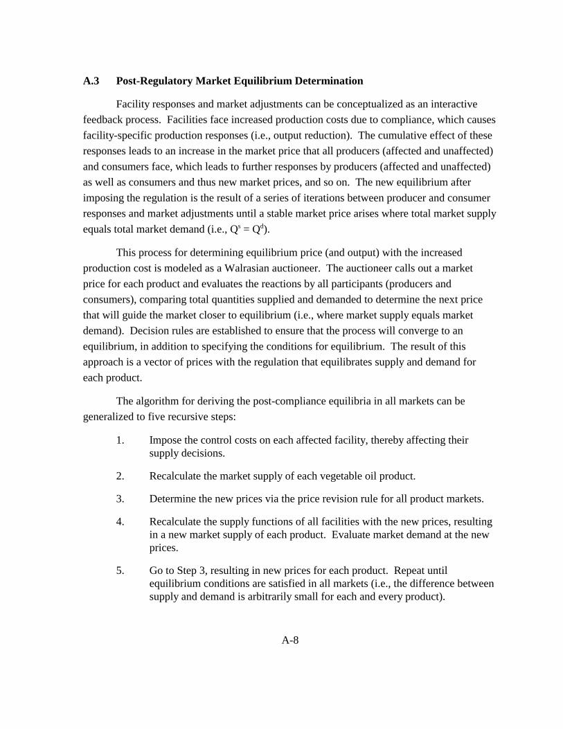
A-8

A.3 Post-Regulatory Market Equilibrium Determination

Facility responses and market adjustments can be conceptualized as an interactive

feedback process. Facilities face increased production costs due to compliance, which causes

facility-specific production responses (i.e., output reduction). The cumulative effect of these

responses leads to an increase in the market price that all producers (affected and unaffected)

and consumers face, which leads to further responses by producers (affected and unaffected)

as well as consumers and thus new market prices, and so on. The new equilibrium after

imposing the regulation is the result of a series of iterations between producer and consumer

responses and market adjustments until a stable market price arises where total market supply

equals total market demand (i.e., Qs = Qd).

This process for determining equilibrium price (and output) with the increased

production cost is modeled as a Walrasian auctioneer. The auctioneer calls out a market

price for each product and evaluates the reactions by all participants (producers and

consumers), comparing total quantities supplied and demanded to determine the next price

that will guide the market closer to equilibrium (i.e., where market supply equals market

demand). Decision rules are established to ensure that the process will converge to an

equilibrium, in addition to specifying the conditions for equilibrium. The result of this

approach is a vector of prices with the regulation that equilibrates supply and demand for

each product.

The algorithm for deriving the post-compliance equilibria in all markets can be

generalized to five recursive steps:

1. Impose the control costs on each affected facility, thereby affecting theirsupply decisions.

2. Recalculate the market supply of each vegetable oil product.

3. Determine the new prices via the price revision rule for all product markets.

4. Recalculate the supply functions of all facilities with the new prices, resultingin a new market supply of each product. Evaluate market demand at the newprices.

5. Go to Step 3, resulting in new prices for each product. Repeat untilequilibrium conditions are satisfied in all markets (i.e., the difference betweensupply and demand is arbitrarily small for each and every product).

A-9

A.4 Economic Welfare Impacts

The economic welfare implications of the market price and output changes of

vegetable oils and related products with the regulations can be examined using two slightly

different tactics, each giving a somewhat different insight but the same implications: changes

in the net benefits of consumers and producers based on the price changes and changes in the

total benefits and costs of these products based on the quantity changes. This analysis

focuses on the first measure—the changes in the net benefits of consumers and producers.

Figure A-2 depicts the change in economic welfare by first measuring the change in

consumer surplus and then the change in producer surplus. In essence, the demand and

supply curves previously used as predictive devices are now being used as a valuation tool.

This method of estimating the change in economic welfare with the regulation divides

society into consumers and producers. In a market environment, consumers and producers of

the good or service derive welfare from a market transaction. The difference between the

maximum price consumers are willing to pay for a good and the price they actually pay is

referred to as “consumer surplus.” Consumer surplus is measured as the area under the

demand curve and above the price of the product. Similarly, the difference between the

minimum price producers are willing to accept for a good and the price they actually receive

is referred to as “producer surplus.” Producer surplus is measured as the area above the

supply curve and below the price of the product. These areas can be thought of as

consumers’ net benefits of consumption and producers’ net benefits of production,

respectively.

In Figure A-2, baseline equilibrium occurs at the intersection of the demand curve, D,

and supply curve, S. Price is Pl with quantity Ql. The increased cost of production with the

regulations will cause the market supply curve to shift upward to S�. The new equilibrium

price of the product is P2. With a higher price for the product there is less consumer welfare,

all else being unchanged. In Figure A-2(a), area A represents the dollar value of the annual

net loss in consumers’ benefits with the increased price. The rectangular portion represents

the loss in consumer surplus on the quantity still consumed, Q2, while the triangular area

represents the foregone surplus resulting from the reduced quantity consumed, Ql–Q2.

In addition to the changes in consumer welfare, there are also changes in producer

welfare with the regulations. With the increase in market price, producers receive higher

revenues on the quantity still purchased, Q2. In Figure A-2(b), area B represents the increase

in revenues due to this increase in price. The difference in the area under the supply curve up

A-10

P1

P2

Q1Q2

S

S’

D

Q/t

$/Q

(a) Change in Consumer Surplus with Regulation

P1

P2

Q1Q2

S

S’

D

Q/t

$/Q

(b) Change in Producer Surplus with Regulation

P1

P2

Q1Q2

S

S’

D

Q/t

$/Q

(c) Net Change in Economic Welfare with Regulation

A

B

C

D

Figure A-2. Economic Welfare Changes with Regulation: Consumer and ProducerSurplus

A-11

to the original market price, area C, measures the loss in producer surplus, which includes the

loss associated with the quantity no longer produced. The net change in producer welfare is

represented by area B–C.

The change in economic welfare attributable to the compliance costs of the regulation

is the sum of consumer and producer surplus changes, that is, – (A) + (B–C). Figure A-2(c)

shows the net (negative) change in economic welfare associated with the regulation as area

D. However, this analysis does not include the benefits that occur outside the market (i.e.,

the value of the reduced levels of air pollution with the regulation). Including this benefit

may reduce the net cost of the regulation or even make it positive.

B-1

APPENDIX B

ESTIMATES OF THE DEMAND AND SUPPLY ELASTICITIES FOR VEGETABLEOILS AND MEALS

This appendix summarizes the demand and supply elasticities used in the economic

impacts model. Because oils and meals for each of corn germ, cottonseed, soybean, and all

other oilseeds combined are modeled individually, estimates of elasticities were required for

each. In cases for which sufficient data were available, EPA estimated the elasticities; in

other cases, the elasticities were obtained directly from the economics literature or assumed

based on similar products’ elasticities.

Section B.1 reviews previous elasticity estimates obtained from the economics

literature. In Section B.2, the elasticity estimation procedure used by EPA is described.

Section B.3 discusses the results of the estimation procedure. Finally, the elasticities used in

the EIA are summarized in Section B.4.

B.1 Review of Previous Elasticity Estimates

The economics literature provides seven sources of estimates of either the demand

elasticities or the supply elasticities for particular vegetable oil or oilseed meal products. The

relevant elasticity estimates from each source are summarized below in reverse chronological

order.

Ugarte (1999)

In developing a national model of the agricultural sector, Ugarte used elasticity

estimates for soybean products as inputs into the analysis. The elasticities used in his model

are based on estimates in the literature. They are as follows:

� soybean meal demand –0.6

� soybean oil demand –0.1

� soybean meal export demand –0.85

� soybean oil export demand –0.75

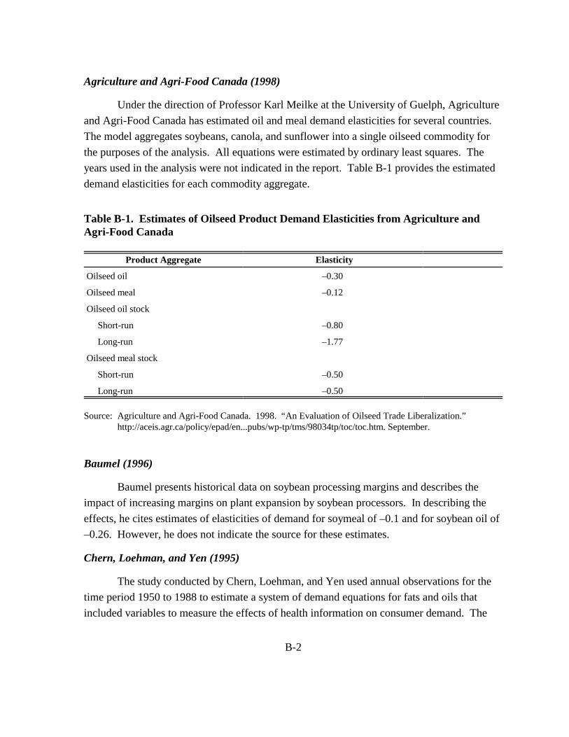
B-2

Agriculture and Agri-Food Canada (1998)

Under the direction of Professor Karl Meilke at the University of Guelph, Agriculture

and Agri-Food Canada has estimated oil and meal demand elasticities for several countries.

The model aggregates soybeans, canola, and sunflower into a single oilseed commodity for

the purposes of the analysis. All equations were estimated by ordinary least squares. The

years used in the analysis were not indicated in the report. Table B-1 provides the estimated

demand elasticities for each commodity aggregate.

Baumel (1996)

Baumel presents historical data on soybean processing margins and describes the

impact of increasing margins on plant expansion by soybean processors. In describing the

effects, he cites estimates of elasticities of demand for soymeal of –0.1 and for soybean oil of

–0.26. However, he does not indicate the source for these estimates.

Chern, Loehman, and Yen (1995)

The study conducted by Chern, Loehman, and Yen used annual observations for the

time period 1950 to 1988 to estimate a system of demand equations for fats and oils that

included variables to measure the effects of health information on consumer demand. The

Table B-1. Estimates of Oilseed Product Demand Elasticities from Agriculture andAgri-Food Canada

Product Aggregate Elasticity

Oilseed oil –0.30

Oilseed meal –0.12

Oilseed oil stock

Short-run –0.80

Long-run –1.77

Oilseed meal stock

Short-run –0.50

Long-run –0.50

Source: Agriculture and Agri-Food Canada. 1998. “An Evaluation of Oilseed Trade Liberalization.”http://aceis.agr.ca/policy/epad/en...pubs/wp-tp/tms/98034tp/toc/toc.htm. September.

B-3

components of their system are butter, corn oil, cottonseed oil, lard, peanut oil, and soybean

oil. Table B-2 provides the estimated demand elasticities for each; standard errors are not

included because the authors did not report them.

The elasticity estimates indicate that all fats and oil products are inelastic, and

cottonseed oil is more elastic than corn oil, peanut oil, and soybean oil. While all of these

results appear reasonable, the estimates of the cross-price elasticities and expenditure

elasticities, which are not reported here, are not. For example, the expenditure elasticities for

corn oil and peanut oil are negative, which would suggest that consumers reduce their

purchases of these products as their income increases. Furthermore, we would expect

vegetable oils to be substitutes for one another, yet cross-price elasticities suggest that many

are complements (e.g., peanut oil and cottonseed oil).

Lence, Hayes, and Meyers (1995)

As part of a model to understand forward trading and storage of soybeans, Lence,

Hayes, and Meyers estimated supply elasticities for soybean oil and meal. The data used to

estimate the model are monthly observations for the period September 1965 through

December 1986, and elasticities are evaluated at the sample means. The estimated supply

elasticities from their “very-short-run” and “short-run” models are presented in Table B-3

along with their standard errors. In either case, the supply elasticities are very inelastic. In

Table B-2. Estimates of Demand Elasticities for Fats and Oils from Chern, Loehman,and Yen Using Annual Data, 1950 to 1988

Product Elasticity

Butter –0.816

Corn oil –0.235


Lard –0.263

Peanut oil –0.242

Soybean oil –0.292

Source: Chern, Wen S., Edna T. Loehman, and Steven T. Yen. 1995. “Information, Health Risk Beliefs, andthe Demand for Fats and Oils.” The Review of Economics and Statistics 77(3):555-64.

B-4

the “very-short-run” model, the elasticities for soybean oil and meal differ, but in the “short-

run” model, they indicate the same supply price responsiveness for each. These differences

likely occur because soybean meal is perishable and more costly to store than soybean oil;

therefore, quantity supplied is less responsive to price changes in the very short run.

Huang (1993)

Huang used annual observations for the time period 1953 to 1990 to estimate

elasticities for the fats and oils subgroup within a complete system of demand equations for

food commodities. The components of the fats and oils subgroup were butter, margarine

(which is produced using vegetable oils), and all other fats and oils. Table B-4 presents the

estimated demand elasticities, standard errors, and percentages of each type in the total fats

and oils consumer budget. All the elasticities indicate that demand is very inelastic for these

products.

Table B-3. Estimates of Supply Elasticities for Soybean Oil and Meal from Lence,Hayes, and Meyers Using Monthly Data, September 1965 to December 1986

ProductVery-Short-Run Supply

ElasticityShort-Run Supply

Elasticity

Soybean oil 0.42(0.10)

0.23(0.09)

Soybean meal 0.11(0.04)

0.23(0.11)

Note: Standard errors are indicated in parentheses.Source: Lence, S.H., D.J. Hayes, and W.H. Meyers. 1995. “The Behavior of Forward-Looking Firms in the

Very Short Run.” American Journal of Agricultural Economics 77(November):922-934.

B-5

Meyers et al. (1993)

The model developed by Meyers et al. estimates supply and demand elasticities for a

number of agricultural crops using annual data from 1965/1970 (the actual year depends on

the crop) through 1992. They calculated elasticities at the average 1985 through 1989 prices

and quantities. Among the commodities included in their analysis are soybean oil and meal.

Table B-5 presents the estimated supply and demand elasticities; standard errors were not

provided in the report and thus are not included here. The demand elasticities are nearly

perfectly inelastic, indicating almost no change in purchases of soybean oil or meal in

response to price changes. The supply elasticities are inelastic as well but larger in absolute

value than the demand elasticities.

Table B-4. Estimates of Demand Elasticities for Fats and Oils from Huang UsingAnnual Data, 1953 to 1990

Type of Product Estimated Elasticity Standard Error

Butter –0.2428 0.1613

Margarine –0.0087 0.1470

Other fats and oils –0.1393 0.0650

Source: Huang, K.S. 1993. U.S. Demand for Food: A Complete System of Price and Income Effects. U.S. Department of Agriculture, Economic Research Service. Bulletin 1821.

Table B-5. Estimates of Demand and Supply Elasticities for Soybean Oil and Mealfrom Meyers et al. Using Annual Data, 1965/1970 to 1992

Product Supply Elasticity Demand Elasticity

Soybean oil 0.660 –0.061

Soybean meal 0.323 –0.097

Source: Meyers, W.H., P. Westhoff, D.L. Stephens, B.L. Buhr, M.D. Helmar, and K.J. Stephens. January1993. “FAPRI U.S. Agricultural Sector Elasticities Volume I: Crops.” Center for Agricultural andRural Development, Iowa State University, Ames, Iowa. Technical Report 92-TR 25.

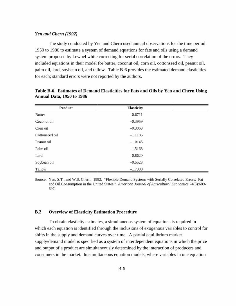
B-6

Yen and Chern (1992)

The study conducted by Yen and Chern used annual observations for the time period

1950 to 1986 to estimate a system of demand equations for fats and oils using a demand

system proposed by Lewbel while correcting for serial correlation of the errors. They

included equations in their model for butter, coconut oil, corn oil, cottonseed oil, peanut oil,

palm oil, lard, soybean oil, and tallow. Table B-6 provides the estimated demand elasticities

for each; standard errors were not reported by the authors.

B.2 Overview of Elasticity Estimation Procedure

To obtain elasticity estimates, a simultaneous system of equations is required in

which each equation is identified through the inclusions of exogenous variables to control for

shifts in the supply and demand curves over time. A partial equilibrium market

supply/demand model is specified as a system of interdependent equations in which the price

and output of a product are simultaneously determined by the interaction of producers and

consumers in the market. In simultaneous equation models, where variables in one equation

Table B-6. Estimates of Demand Elasticities for Fats and Oils by Yen and Chern UsingAnnual Data, 1950 to 1986

Product Elasticity

Butter –0.6711

Coconut oil –0.3959

Corn oil –0.3063


Peanut oil –1.0145

Palm oil –1.5168

Lard –0.8620

Soybean oil –0.5523

Tallow –1.7380

Source: Yen, S.T., and W.S. Chern. 1992. “Flexible Demand Systems with Serially Correlated Errors: Fatand Oil Consumption in the United States.” American Journal of Agricultural Economics 74(3):689-697.

B-7

feed back into variables in another equation, the error terms are correlated with the

endogenous variables (price and output). In comparison, single-equation ordinary least

squares (OLS) estimation of individual equations will lead to biased and inconsistent

parameter estimates because it does not account for the correlation of the error term with the

endogenous variables.

Exogenous variables influencing the demand for vegetable oils and oilseed meals

include measures of general economic activity (such as U.S. gross domestic product [GDP]),

population, and the prices of substitutes. Exogenous variables influencing the level of supply

of vegetable oils and oilseed meals include measures of the change in the costs of production

caused by changes in prices of key inputs like oilseeds, fuel, electricity, and labor.

The supply/demand system for each vegetable oil and oilseed meal at the wholesale

level can be defined as follows:

Qtd = f(Pt,Zt) + ut (B.1)

Qts = g(Pt,Wt) + vt (B.2)

Qtd = Qt

s (B.3)

Eq. (B.1) shows per capita quantity demanded as a function of price, Pt; a vector of demand

shifters, Zt (e.g., measures of economic activity and substitute prices); and an error term, ut.

Eq. (B.2) represents quantity supplied as a function of price and a vector of supply shifters,

Wt (e.g., input prices), and an error term, vt, while Eq. (B.3) specifies the equilibrium

condition that quantity supplied equals quantity demanded, creating a system of three

equations with three endogenous variables. The interaction of the specified market forces

solves this system, generating equilibrium values for the variables Pt* and Qt

*=Qtd*=Qt

s*.

To generate estimates separately of either the demand elasticities or the supply

elasticities, the two-stage least squares (2SLS) regression procedure can also be used. The

first stage of the 2SLS procedure involves regressing the observed price against the supply

and demand “shifter” variables that are exogenous to the system. This first stage produces

fitted (or predicted) values for the price variable that are, by definition, highly correlated with

the true endogenous variable, the observed price, and uncorrelated with the error term. In the

second stage, these fitted values are then employed as observations of the right-hand side

price variable in the demand function. These fitted values are uncorrelated with the error

term by construction and thus do not incur the endogeneity bias. By converting all variables

B-8

into natural logarithms, each coefficient on the price variable yields an estimate of the

constant elasticity of demand or supply for each vegetable oil or oilseed meal product.

Elasticities estimated in this manner for vegetable oil and oilseed meals were used in the

economic impacts model.

B.3 Results of Elasticity Estimation

The data used in the elasticity estimation for vegetable oils and meals are annual

time-series data covering the period 1984 through 1996 and were obtained primarily from

USDA publications, including Agricultural Statistics, Oil Crops Yearbook, Oil Crops

Situation and Outlook, and Sugar and Sweetener Yearbook.

B.3.1 Demand Equation Estimation

Demand equations were estimated using a general specification where the per capita

quantity consumed is expressed as a function of own-price, per capita income (for oil

products but not meal products), price of the primary substitute, trend, and trend squared.

Trend and trend squared were included as a general way to model the effects of changes in

tastes and preferences for vegetable oils and oilseed meals. All variables were converted to

natural logs, and all price and income variables were deflated by the implicit GDP deflator.

The endogenous variables in the equations are per capita consumption, own-price, and the

price of the primary substitute. The price of the primary substitute was included as an

endogenous variable because oil products substitute readily for one another as do meal

products; therefore, consumption of each is jointly determined with the price of its

substitutes. The exogenous variables include per capita income, trend, and trend squared.

The list of instruments includes these exogenous variables in addition to supply factors

influencing the price of the product: the price of the oilseed input, wages at the three-digit

SIC level, and the producer price index for fuel.

Using this model, reasonable estimates were obtained for cottonseed oil, cottonseed

meal, soybean oil, and soybean meal. For corn oil, none of the regressors in the model are

significant other than its price and trend. Dropping all of the other regressors in the model

results in a reasonable estimate of the demand elasticity and a reasonable adjusted R2. The

results of these five models are provided in Table B-7.

Sufficient data were not available to estimate a demand equation for corn germ meal.

Sufficient data were available to estimate demand for linseed oil, linseed meal, sunflower oil,

and sunflower meal, but the data series are too volatile to obtain reasonable estimates. Thus,

B-9

Table B-7. Results of Econometric Estimation of Oilseed Product Demand Equations

DependentVariable—Regressor

Corn Oil Cottonseed OilCottonseed

Meal Soybean Oil Soybean Meal

Per CapitaCorn Oil

Consumption

Per CapitaCottonseed OilConsumption

Per CapitaCottonseed

MealConsumption

Per CapitaSoybean Oil

Consumption

Per CapitaSoybean MealConsumption

Intercept 2.640(4.38)

–14.249(–1.37)

–2.682(–0.43)

3.927(1.46)

5.287(33.95)

Price –0.387(–2.22)

–0.245(–0.32)

–1.011(–1.60)

–0.340(–1.92)

–0.268(–0.75)

Substitute pricea — –3.635(–1.32)

1.517(0.99)

0.133(0.19)

0.178(0.51)

Income — 0.537(0.77)

— 0.412(2.07)

—

Trend 0.016(2.61)

0.212(2.80)

0.032(0.70)

0.035(1.80)

0.021(1.63)

Trend squared — –0.008(–2.19)

–0.002(–0.76)

–0.001(–1.27)

0.001(0.07)

Adjusted R2 0.722 0.7305 0.643 0.885 0.895

Durbin-Watson 2.753 2.050 2.527 2.001 2.282

Observations 13 13 13 13 13

Notes:1. Numbers in parentheses are t-ratios (coefficient estimate divided by its standard error).2. All variables are in natural logs.

a Substitute commodity prices used were as follows:cottonseed oil equation: soybean oilcottonseed meal equation: producer price index for animal feedsoybean oil equation: cottonseed oilsoybean meal equation: cottonseed meal

B-10

elasticities for corn germ meal and the other oilseed products were assumed based on the

available estimates.

B.3.2 Supply Equation Estimation

Supply equations were estimated using a general specification where quantity was

expressed as a function of price, wages at the three-digit SIC level, the price of the oilseed

input, and the price index for fuel. All variables were converted to natural logs, and all price

variables were deflated by the implicit GDP deflator. The endogenous variables in the

equations are price and quantity, and all others are assumed exogenous. The list of

instruments includes these exogenous variables in addition to demand factors influencing the

price of the product: income, price of substitutes, trend, and trend squared.

Reasonable estimates of the supply elasticities were not obtained and thus are not

reported here. Supply of these products is most likely a more complicated process than can

be represented by this simple model. In particular, inventories of products likely influence

the supply response of producers. As a result, supply elasticity estimates used in the EIA

were chosen based on values from the economics literature for soybean oil and meal.

B.4 Results of Elasticity Estimation

Table B-8 summarizes the domestic demand and supply elasticities and the trade

elasticities from the literature and from independent econometric estimates. In addition, the

elasticities used in the EIA are indicated. Corn oil and soybean demand elasticities used in

the EIA were obtained directly from the econometric estimates because they are similar to

those reported in the literature. The cottonseed demand elasticity used in the EIA is the

middle value of the econometrically estimated and reported values because the

econometrically estimated elasticity fell outside the range of reported values. The demand

elasticity for all other oils is a simple average of the three elasticities for the other oils.

Cottonseed meal and soybean meal demand elasticities were obtained directly from the

econometric estimates. The soybean meal estimate from the literature is similar to the

econometric estimate, and no estimates for cottonseed meal were available from the

literature. The demand elasticity used for corn germ meal and all other meals is a simple

average of the cottonseed meal and soybean meal econometric estimates.

The supply elasticities for oils and meals are based on estimates in the literature for

soybean oil and meal. For each of these products, two estimates were available; thus, the

elasticities used in

B-11

Table B-8. Summary of Elasticity Estimates for Vegetable Oils and Meals

ProductLiteratureEstimates

EconometricEstimates

Elasticity Usedfor the EIA

DemandElasticities

Corn oil –0.235, –0.306 –0.387 –0.39

Cottonseed oil –0.646, –1.118 –0.245 –0.65

Soybean oil -0.292, -0.610,-0552, -0.1a

–0.340 –0.34

All other oils –0.242 (peanut)–1.014 (peanut)

–0.33b

Corn germ meal –0.46

Cottonseed meal –1.011 –1.01

Soybean meal –0.097, -0.6a –0.268 –0.27

All other meals –0.64c

SupplyElasticities

Corn oil 0.44d

Cottonseed oil 0.44d

Soybean oil 0.660, 0.230 0.44d

All other oils 0.44d

Corn germ meal 0.28e

Cottonseed meal 0.28e

Soybean meal 0.323, 0.230 0.28e

All other meals 0.28e

Import SupplyElasticities

All products 1.00f

Export DemandElasticities

All products –1.00f

a Value was used in a model developed by Ugarte but was not econometrically estimated.b Average of corn oil, cottonseed oil, and soybean oil econometric estimates.c Average of cottonseed meal and soybean meal econometric estimates.d Midpoint of soybean oil supply elasticities from the literature.e Midpoint of soybean meal supply elasticities from the literature.f Value is assumed.

B-12

the EIA are an average of the elasticities from each source. For lack of other information, the

soybean elasticities were used for the cottonseed, corn germ, and all other oils and meals as

well.

In general, trade elasticities are expected to be more elastic than domestic supply and

demand elasticities. Except for soybean oil and meal export demand, elasticity values are not

available from either econometric estimates or the literature. For these soybean products,

however, the values reported by Ugarte are assumed rather than econometrically estimated.

Thus, the values of –1 and 1 are assumed for the export demand and import supply

elasticities respectively for all vegetable oil and meal products.

C-1

APPENDIX C

ECONOMIC MODEL SENSITIVITY ANALYSIS

A sensitivity analysis was conducted to determine the effects of different demand and

supply elasticity estimates under the MACT floor regulatory alternative promulgated by the

EPA. This analysis assumes lost production costs. Table C-1 presents the sets of elasticities

used in the analysis reported in Section 4 and for two sensitivity analyses. Sensitivity

Analysis A uses the most inelastic demand elasticities and the most elastic supply elasticities

from the literature (see Table B-6). These elasticities are expected to result in the greatest

predicted changes in consumer and producer surplus and the greatest social costs of the

regulation. Sensitivity Analysis B uses the most elastic demand elasticities and the most

inelastic supply elasticities from the literature. Likewise, these elasticities are expected to

result in the smallest predicted changes.

The following results are presented:

� market-level impacts of the NESHAP (Table C-2),

� industry-level impacts of the NESHAP (Table C-3),

� distribution of industry impacts of the NESHAP by profit losers and profit gainers(Table C-4),

� distribution of the social costs associated with the NESHAP (Table C-5), and

� small business impacts of the NESHAP (Table C-6).

In general, the projected effects of the regulation are not particularly sensitive to changes in

the elasticity values. However, predicted price, output, trade, revenue, and consumer and

producer surplus are greater under Sensitivity Analysis A relative to the base values and less

under Sensitivity Analysis B.

C-2

Table C-1. Summary of Market-Level Impacts of Vegetable Oil Production NESHAP: 1995

Primary Sensitivity Analysis Aa Sensitivity Analysis Bb

Demand Supply Demand Supply Demand Supply

Oils

Corn –0.39 0.44 –0.235 0.66 –0.39 0.23

Cottonseed –0.65 0.44 –0.245 0.66 –1.118 0.23

Soybean –0.34 0.44 –2.92 0.66 –0.61 0.23

All Other –0.46 0.44 –0.257c 0.66 –1.044 0.23

Meals

Corn Germ –0.64d 0.28 –0.55d 0.32 –0.64d 0.23

Cottonseed –1.01 0.28 –1.01 0.32 –1.01 0.23

Soybean –0.27 0.28 –0.097 0.32 –0.268 0.23

All Other –0.64d 0.28 –0.55d 0.32 –0.64d 0.23

a Inelastic demand/elastic supply.b Elastic demand/inelastic supply.c Average of corn, cottonseed, soybean.d Average of cottonseed, soybean.

C-3

Table C-2. Summary of Market-Level Impacts of Vegetable Oil Production NESHAP: 1995

Inelastic Demand/Elastic Supply Primary

Elastic Demand/Inelastic Supply

Changes from Baseline

Scenario Baseline Absolute Percent Absolute Percent Absolute Percent

Corn OilMarket Price ($/short ton) $532.00 $3.40 0.64% $2.53 0.48% $1.65 0.31%Market Output (tpy) 1,126,198 –3,705 –0.33% –3,280 –0.29% –2,141 –0.19%Domestic Production 1,121,703 –3,734 –0.33% –3,301 –0.29% –2,155 –0.19%

Solvent Extraction 1,066,819 –3,965 –0.37% –3,416 –0.32% –2,194 –0.21%Mechanical Extraction 54,884 232 0.42% 115 0.21% 39 0.07%

Exports 415,270 –2,640 –0.64% –1,966 –0.47% –1,282 –0.31%Imports 4,495 29 0.64% 21 0.48% 14 0.31%

Cottonseed OilMarket Price ($/short ton) $536.00 $4.14 0.77% $2.55 0.48% $1.18 0.22%Market Output (tpy) 646,031 –2,070 –0.32% –2,233 –0.35% –1,551 –0.24%Domestic Production 645,925 –2,071 –0.32% –2,234 –0.35% –1,552 –0.24%

Solvent Extraction 622,308 –2,191 –0.35% –2,283 –0.37% –1,564 –0.25%Mechanical Extraction 23,617 120 0.51% 49 0.21% 12 0.05%

Exports 147,281 –1,130 –0.77% –697 –0.47% –324 –0.22%Imports 106 1 0.77% 1 0.48% 0 0.22%

Soybean OilMarket Price ($/short ton) $536.00 $2.29 0.43% $1.84 0.34% $0.94 0.17%Market Output (tpy) 7,981,880 –13,370 –0.17% –11,867 –0.15% –9,285 –0.12%Domestic Production 7,968,264 –13,428 –0.17% –11,914 –0.15% –9,309 –0.12%

Solvent Extraction 7,968,264 –13,428 –0.17% –11,914 –0.15% –9,309 –0.12%Mechanical Extraction 0 0 NA 0 NA 0 NA

Exports 1,143,544 –4,864 –0.43% –3,905 –0.34% –1,996 –0.17%Imports 13,616 58 0.43% 47 0.34% 24 0.17%

(continued)

C-4

Table C-2. Summary of Market-Level Impacts of Vegetable Oil Production NESHAP: 1995 (Continued)





All Other Vegetable OilsMarket Price ($/short ton) $658.82 $1.57 0.24% $1.07 0.16% $0.48 0.07%Market Output (tpy) 1,623,013 –2,112 –0.13% –1,763 –0.11% –1,214 –0.07%Domestic Production 1,093,411 –3,374 –0.31% –2,622 –0.24% –1,600 –0.15%


Exports 632,625 –1,506 –0.24% –1,025 –0.16% –461 –0.07%Imports 529,602 1,262 0.24% 859 0.16% 386 0.07%

Corn Germ MealMarket Price ($/short ton) $88.40 $0.36 0.41% $0.30 0.34% $0.26 0.30%Market Output (tpy) 1,473,651 –3,447 –0.23% –3,304 –0.22% –2,868 –0.19%Domestic Production 1,473,651 –3,447 –0.23% –3,304 –0.22% –2,868 –0.19%

Solvent Extraction 1,401,546 –3,542 –0.25% –3,373 –0.24% –2,918 –0.21%Mechanical Extraction 72,105 95 0.00% 69 49 0.00%

Exports 61,950 –254 –0.41% –212 –0.34% –184 –0.30%Imports 0 0 NA 0 NA 0 NA

Cottonseed MealMarket Price ($/short ton) $123.20 $0.37 0.30% $0.34 0.27% $0.29 0.23%Market Output (tpy) 1,826,100 –5,561 –0.30% –5,019 –0.27% –4,292 –0.24%Domestic Production 1,826,100 –5,561 –0.30% –5,019 –0.27% –4,292 –0.24%


Exports 89,700 –271 –0.30% –244 –0.27% –209 –0.23%Imports 0 0 NA 0 NA 0 NA

(continued)

C-5

Table C-2. Summary of Market-Level Impacts of Vegetable Oil Production NESHAP: 1995 (Continued)





Soybean MealMarket Price ($/short ton) $173.80 $0.62 0.36% $0.47 0.27% $0.42 0.24%Market Output (tpy) 31,290,977 –32,124 –0.10% –35,793 –0.11% –31,689 –0.10%Domestic Production 31,225,572 –32,359 –0.10% –35,970 –0.12% –31,846 –0.10%

Solvent Extraction 31,225,572 –32,359 –0.10% –35,970 –0.12% –31,846 –0.10%Mechanical Extraction 0 0 NA 0 NA 0 NA

Exports 6,491,570 –23,210 –0.36% –17,571 –0.27% –15,509 –0.24%Imports 65,405 235 0.36% 178 0.27% 157 0.24%

All Other Vegetable OilMealsMarket Price ($/short ton) $93.22 $0.12 0.13% $0.10 0.10% $0.08 0.09%Market Output (tpy) 2,520,129 –1,810 –0.07% –1,729 –0.07% –1,459 –0.06%Domestic Production 1,583,559 –2,982 –0.19% –2,704 –0.17% –2,282 –0.14%


Exports 138,469 –173 –0.12% –144 –0.10% –122 –0.09%Imports 936,570 1,172 0.13% 975 0.10% 823 0.09%

NA = Not available.

C-6

Table C-3. Summary of Industry-Level Impacts of Vegetable Oil Production NESHAP: 1995





Total Industry

Revenues ($103) $11,963,996 $27,959 0.2% $17,728 0.1% $10,048 0.1%

Costs ($103) $10,698,845 –$6,926 –0.1% –$6,394 –0.1% –$2,888 –0.0%

Post-regulatory $0 $12,056 NA $12,076 NA $12,102 NA

Oil and Meal Production $10,698,845 –$18,982 –0.2% –$18,470 –0.2% –$14,989 –0.1%

Gross Profits ($103) $1,265,151 $34,885 2.8% $24,122 1.7% $12,936 0.8%

Operating Entities

Product Line-Closures NA 0 NA 0 NA 0 NA

Facility Closures NA 0 NA 0 NA 0 NA

Employment Loss NA –15 NA –12 NA –6 NA

Solvent Extraction

Revenues ($103) $11,853,542 $27,222 0.2% $17,264 0.1% $9,802 0.1%

Costs ($103) $10,611,376 –$7,089 –0.1% –$6,477 –0.1% –$2,923 –0.0%


Production $10,611,376 –$19,145 –0.2% –$18,554 –0.2% –$15,025 –0.1%

Gross Profits ($103) $1,242,166 $34,310 2.8% $23,741 1.7% $12,725 0.8%

Operating Entities

Product Lines 111 0 0.0% 0 0.0% 0 NA

Facilities 106 0 0.0% 0 0.0% 0 NA

Employment 5,673 –15 –0.3% –12 –0.2% –6 NA

(continued)

C-7

Table C-3 Summary of Industry-Level Impacts of Vegetable Oil Production NESHAP: 1995 (Continued)





Mechanical Extraction

Revenues ($103) $110,454 $737 0.7% $464 0.4% $246 0.2%

Costs ($103) $87,469 $162 0.2% $84 0.1% $36 0.0%

Post-regulatory $0 $0 0.0% $0 0.0% $0 0.0%

Production $87,469 $162 0.2% $84 0.1% $36 0.0%

Gross Profits ($103) $22,985 $574 2.5% $380 1.5% $211 0.7%

Operating Entities

Product Lines NA NA NA NA NA NA NA

Facilities NA NA NA NA NA NA NA

Employment NA NA NA NA NA NA NA

NA = Not available.

C-8

Table C-4. Summary of Distributional Industry Impacts of the Vegetable Oil Production NESHAP: 1995

Floor

Supply Elasticity Inelastic Demand/Elastic Supply Primary Elastic Demand/Inelastic Supply

Solvent Extraction Facilities

With Profit Loss

With Profit Gain Total

With Profit Loss


With Profit Loss


Number 17 89 106 21 85 106 32 74 106

Facility Capacity (tonsper day)

Total 8,062 165,141 173,203 11,362 161,841 173,203 24,977 148,226 173,203

Per Facility 474 1,856 1,634 541 1,904 1,634 781 2,003 1,634

Annual Solvent Loss

Total (103 gallons) 1,584 14,412 15,996 2,419 13,577 15,996 3,981 12,015 15,996

Gallons per Ton ofOilseed

0.86 0.29 0.31 0.84 0.28 0.31 0.70 0.27 0.31

IncrementalCompliance Costs

Total ($103/yr) $1,867 $10,284 $12,151 $2,502 $9,649 $12,151 $3,808 $8,343 $12,151

Per Ton of Oilseed $1.01 $0.21 $0.24 $0.87 $0.20 $0.24 $0.67 $0.19 $0.24

Change in GrossProfits ($103/yr)a

–$1,038 $35,349 $34,310 –$1,184 $24,925 $23,741 –$1,473 $14,198 $12,725

Change inEmployment (FTEs)b

–8 –7 –15 –7 –5 –12 –3 –3 –6

a Gross profits calculated as revenue less costs of production including oilseed costs.b FTEs = Full-time equivalents.

C-9

Table C-5. Distribution of the Social Costs Associated with the Vegetable OilProduction NESHAP: 1995

Floor with Lost Production Costs

InelasticDemand/Elastic

Supply Primary

ElasticDemand/Inelastic

Supply

Social Cost Component Change in Value ($103)

Consumer Surplus –$48,321 –$36,929 –$25,007

Corn Oil –$3,827 –$2,845 –$1,854

Cottonseed Oil –$2,673 –$1,644 –$763

Soybean Oil –$18,259 –$14,649 –$7,476

All Other Vegetable Oils –$2,548 –$1,734 –$779

Corn Germ Feed –$537 –$446 –$387

Cottonseed Meal –$680 –$613 –$524

Soybean Meal –$19,504 –$14,752 –$13,017

All Other Vegetable Meals –$294 –$244 –$206

Producer Surplus $35,915 $24,846 $13,314

Domestic Producers $34,885 $23,122 $12,936

Solvent Extraction $34,310 $23,741 $12,725

Mechanical Extraction $574 $380 $211

Foreign Producers $1,030 $725 $379

Social Costs of Regulation –$12,407 -$12,083 –$11,693

C-10

Table C-6. Summary of Small Business Impacts of Vegetable Oil Production NESHAP: 1995

Floor with Lost Production Costs

Inelastic Demand/ElasticSupply Primary

Elastic Demand/InelasticSupply


Baseline Absolute Percent Absolute Percent Absolute Percent

Revenues ($103) $780,636 -$396 –0.1% –$793 –0.1% –$739 –0.1%

Costs ($103) $665,767 –$1,507 –0.2% –$1,010 –0.2% –$185 –0.1%


Production $665,767 –$3,633 –0.5% –$3,141 –0.5% –$2,324 –0.4%

Gross Profits ($103) $114,869 $1,111 1.1% $217 0.2% –$554 –0.4%

Operating Entities

Product Lines 21 0 0.0% 0 0.0% 0 0.0%

Facilities 20 0 0.0% 0 0.0% 0 0.0%

Employment NR –7 NR –6 NR –2 NR

NA = Not available.NR = Not reported to avoid disclosure of CBI.

Economic Impact Analysis for the Final Vegetable Oil Processing ...

Documents

Transcript of Economic Impact Analysis for the Final Vegetable Oil Processing ...