Economic Growth: Extensions - Discover Economics to the Solow Growth Model 1. ... India Indonesia...

1

Economic Growth: ExtensionsEconomic Growth: Extensions

2

ECN 101 MACROECONOMICSECN 101 MACROECONOMICS slide 1

Road Map to this LectureRoad Map to this Lecture1. Extensions to the Solow Growth Model

1. Population Growth2. Technological growth3. The Golden Rule

2. Endogenous Growth Theory1. Human capital and increasing returns to

scale

3


Population GrowthPopulation GrowthAssume that the population (labor force) grow at rate n. (n is exogenous)

L nL∆

=

E.g.: Suppose L = 1000 in year 1 and the population is growing at 2%/year (n = 0.02).

Then ∆L = n L = 0.02 × 1000 = 20,so L = 1020 in year 2.

4


BreakBreak--even investmenteven investment(δ +n)k = break-even investment,

the amount of investment necessary to keep k constant.

Break-even investment includes:

δk to replace capital as it wears out

nk to equip new workers with capital(otherwise, k would fall as the existing capital stock would be spread more thinly over a larger population of workers)

5


The equation of motion for The equation of motion for kkWith population growth, the equation of motion for k is

∆k = s f(k) − (δ +n)k

break-even investment

actual investment

6


The Solow Model diagramThe Solow Model diagram

Investment, break-even investment

Capital per worker, k

sf(k)

(δ+ n )k

k*

∆k = s f(k) − (δ +n)k

7


The impact of population growthThe impact of population growth



sf(k)

(δ+n1)k

k1*

(δ+n2)k

k2*

An increase in ncauses an increase in break-even investment,leading to a lower steady-state level of k.

8


Prediction:Prediction:

Higher n ⇒ lower k*.

And since y = f(k) , lower k* ⇒ lower y* .

Thus, the Solow model predicts that countries with higher population growth rates will have lower levels of capital and income per worker in the long run.

9


Chad

Kenya

Zimbabwe

Cameroon

Pakistan

Uganda

India

Indonesia

IsraelMexico

Brazil

Peru

Egypt

Singapore

U.S.

U.K.

Canada

FranceFinlandJapan

Denmark

IvoryCoast

Germany

Italy

100,000

10,000

1,000

1001 2 3 40

Income per person in 1992(logarithmic scale)

Population growth (percent per year) (average 1960 –1992)

International Evidence on Population International Evidence on Population Growth and Income per PersonGrowth and Income per Person

10


The Golden Rule with Population GrowthThe Golden Rule with Population Growth

To find the Golden Rule capital stock, we again express c* in terms of k*:

c* = y* − i*

= f (k*) − (δ +n)k*

c* is maximized when MPK = δ + n

or equivalently, MPK − δ = n

In the Golden Rule Steady State,

the marginal product of capital net of

depreciation equals the population growth rate.

In the Golden In the Golden Rule Steady State, Rule Steady State,

the marginal product of the marginal product of capital net of capital net of

depreciation equals the depreciation equals the population growth rate.population growth rate.

11


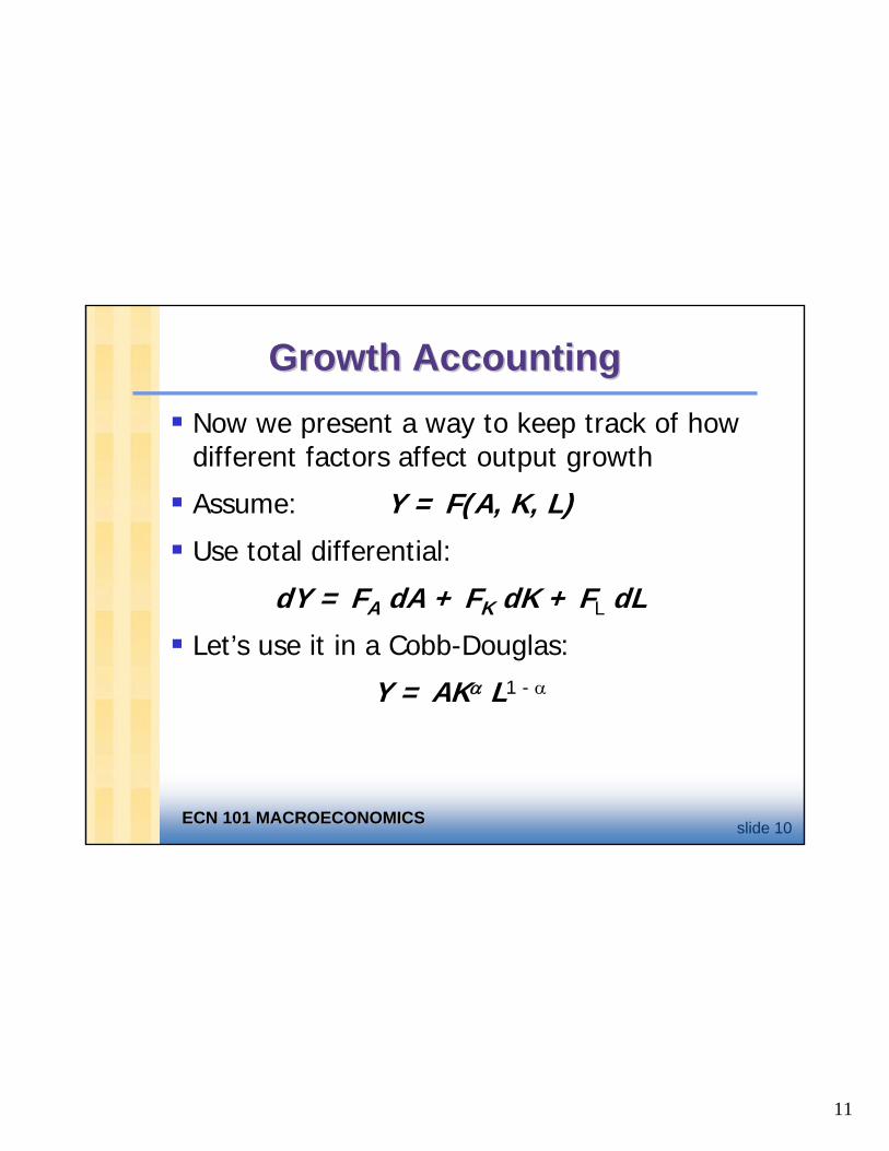
Growth AccountingGrowth AccountingNow we present a way to keep track of how different factors affect output growth

Assume: Y = F(A, K, L)

Use total differential:

dY = FA dA + FK dK + FL dL

Let’s use it in a Cobb-Douglas:

Y = AKα L1 - α

12


Growth Accounting, cont.Growth Accounting, cont.Notice that for the Cobb-Douglas– FA = Y/A– FK = α Y/K– FL = (1 - α) Y/L

Hence:

13


Growth Accounting, cont.Growth Accounting, cont.Notice

dY/Y ≅ ∆ Y/Y ≅ %change in Y

From the previous derivations:

%∆ Y = %∆ TFP + % ∆ K + % ∆ L

In the U.S., α ≅ 0.3 and 1 - α ≅ 0.7

14


U.S. Growth AccountingU.S. Growth Accounting

0.91.61.23.71990-99

0.61.61.23.41980-90

1.01.21.43.61970-80

1.81.21.44.41960-70

1.31.01.03.31950-60

∆ A/A(1 - α) ∆ L/Lα ∆ K/K∆ Y/YYears

SOURCE OF GROWTH(avg. % increase p. year)

15


TechnologyTechnologySo far,

the production technology is held constantincome per capita is constant in the steady state.

However, neither is true in the real world:1929-2001: U.S. real GDP per person grew by a factor of 4.8, or 2.2% per year. examples of technological progress abound…

16


Examples of technological progressExamples of technological progress

The real price of computer power has fallen an average of 30% per year over the past three decades.

The average car built in 1996 contained more computer processing power than the first lunar landing craft in 1969.

Modems are 22 times faster today than two decades ago.

Since 1980, semiconductor usage per unit of GDP has increased by a factor of 3,500.

1981: 213 computers connected to the Internet2000: 60 million computers connected to the Internet

17


Tech. progress in the Solow modelTech. progress in the Solow model

A new variable: E = labor efficiency

Assume: Technological progress is labor-augmenting: it increases labor efficiency at the exogenous rate g:

EgE∆

=

18



We now write the production function as:

where L ×E = the number of effective workers. – Hence, increases in labor efficiency have

the same effect on output as increases in the labor force.

( , )Y F K L E= ×

19


Tech. progress in the Solow modelTech. progress in the Solow modelNotation:

y = Y/LE = output per effective worker k = K/LE = capital per effective worker

Production function per effective worker:y = f(k)

Saving and investment per effective worker:s y = s f(k)

20


Tech. progress in the Solow modelTech. progress in the Solow model(δ + n + g)k = break-even investment:

the amount of investment necessary to keep k constant.

Consists of:δk to replace depreciating capital

n k to provide capital for new workers

g k to provide capital for the new “effective” workers created by technological progress

21





sf(k)

(δ+n +g )k

k*

∆k = s f(k) − (δ +n +g)k

22


SteadySteady--State Growth Rates in the State Growth Rates in the Solow Model with Tech. ProgressSolow Model with Tech. Progress

n + gY = y ×E ×L Total output

g(Y/L ) = y ×E Output per worker

0y = Y/ (L ×E )Output per effective worker

0k = K/ (L ×E )Capital per effective worker

Steady-state growth rateSymbolVariable

23


The Golden RuleThe Golden RuleTo find the Golden Rule capital stock, express c* in terms of k*:

c* = y* − i*

= f (k*) − (δ +n +g)k*

c* is maximized when MPK = δ + n + g

or equivalently, MPK − δ = n + g

In the Golden Rule Steady State,

the marginal product of capital

net of depreciation equals the

pop. growth rate plus the rate of tech progress.

In the Golden In the Golden Rule Steady State, Rule Steady State,

the marginal the marginal product of capital product of capital

net of depreciation net of depreciation equals the equals the

pop. growth rate pop. growth rate plus the rate of plus the rate of tech progress.tech progress.

24


Evaluating the Rate of SavingEvaluating the Rate of SavingUse the Golden Rule to determine whether our saving rate and capital stock are too high, too low, or about right.

To do this, we need to compare (MPK − δ ) to (n + g ).

If (MPK − δ ) > (n + g ), then we are below the Golden Rule steady state and should increase s.

If (MPK − δ ) < (n + g ), then we are above the Golden Rule steady state and should reduce s.

25


Evaluating the Rate of SavingEvaluating the Rate of SavingTo estimate (MPK − δ ), we use

three facts about the U.S. economy:

1. k = 2.5 yThe capital stock is about 2.5 times one year’s GDP.

2. δ k = 0.1 yAbout 10% of GDP is used to replace depreciating capital.

3. MPK×k = 0.3 yCapital income is about 30% of GDP

26


Evaluating the Rate of SavingEvaluating the Rate of Saving1. k = 2.5 y

2. δ k = 0.1 y

3. MPK × k = 0.3 y

0 12 5..

k yk yδ

= 0 10 04

2 5.

..

δ = =⇒

To determine δ , divide 2 by 1:

27


Evaluating the Rate of SavingEvaluating the Rate of Saving1. k = 2.5 y

2. δ k = 0.1 y

3. MPK × k = 0.3 y

MPK 0 32 5..

k yk y×

= 0 3MPK 0 12

2 5.

..

= =⇒

To determine MPK, divide 3 by 1:

Hence, MPK − δ = 0.12 − 0.04 = 0.08

28


Evaluating the Rate of SavingEvaluating the Rate of SavingFrom the last slide: MPK − δ = 0.08

U.S. real GDP grows an average of 3%/year, so n + g = 0.03

Thus, in the U.S.,MPK − δ = 0.08 > 0.03 = n + g

Conclusion:

The U.S. is below the Golden Rule steady state: The U.S. is below the Golden Rule steady state: if we increase our saving rate, we will have faster if we increase our saving rate, we will have faster growth until we get to a new steady state with growth until we get to a new steady state with higher consumption per capita.higher consumption per capita.

29


Effects of Increases in Parameters on the Solow Effects of Increases in Parameters on the Solow Growth ModelGrowth Model

IncreasesIncreasesUpUpDecreasesg

No changeNo changeDownDownDecreasesδ

No changeIncreasesDownUpDecreasesn

No changeNo changeUpUpIncreasess

Permanent Growth Rate of Y/L

Permanent Growth Rate of Y

Level of Y/L

Level of Y

Equilibrium K/Y

The Effect on…When there is an increase in the parameter…

30


Policies to increase the saving ratePolicies to increase the saving rateReduce the government budget deficit(or increase the budget surplus)

Increase incentives for private saving:reduce capital gains tax, corporate income tax, estate tax as they discourage savingreplace federal income tax with a consumption taxexpand tax incentives for IRAs (individual retirement accounts) and other retirement savings accounts

31


Allocating the economyAllocating the economy’’s investments investment

In the Solow model, there’s one type of capital.

In the real world, there are many types,which we can divide into three categories:– private capital stock– public infrastructure– human capital: the knowledge and skills

that workers acquire through education

How should we allocate investment among these types?

32


Allocating the economyAllocating the economy’’s investment: s investment: two viewpointstwo viewpoints

1. Equalize tax treatment of all types of capital in all industries, then let the market allocate investment to the type with the highest marginal product.

2. Industrial policy: Govt should actively encourage investment in capital of certain types or in certain industries, because they may have positive externalities (by-products) that private investors don’t consider.

33


Possible problems with industrial policyPossible problems with industrial policy

The govt may not have the ability to “pick winners” (choose industries with the highest return to capital or biggest externalities).

Concern that politics (e.g. campaign contributions) rather than economics would influence which industries get preferential treatment.

34


4. Encouraging technological progress4. Encouraging technological progress

Patent laws:encourage innovation by granting temporary monopolies to inventors of new products

Tax incentives for R&D

Grants to fund basic research at universities

Industrial policy: encourage specific industries that are key for rapid tech. progress (subject to the concerns on the preceding slide)

35


CASE STUDY: CASE STUDY: The Productivity SlowdownThe Productivity Slowdown

1.5

1.8

2.6

2.3

2.0

1.6

1.8

2.2

2.4

8.2

4.9

5.7

4.3

2.9

1972-951948-72

U.S.

U.K.

Japan

Italy

Germany

France

Canada

Growth in output per person(percent per year)

36


Possible explanationsPossible explanations

Measurement problemsIncreases in productivity not fully measured.– But: Why would measurement problems

be worse after 1972 than before?

Oil pricesOil shocks occurred about when productivity slowdown began.– But: Then why didn’t productivity speed up

when oil prices fell in the mid-1980s?

37


Possible explanationsPossible explanations

Worker quality1970s - large influx of new entrants into labor force (baby boomers, women).New workers are less productive than experienced workers.

The depletion of ideasPerhaps the slow growth of 1972-1995 is normal and the true anomaly was the rapid growth from 1948-1972.

38


CASE STUDY: CASE STUDY: I.T. and the I.T. and the ““new economynew economy””

2.9

2.5

1.1

4.7

1.7

2.2

2.7

1.5

1.8

2.6

2.3

2.0

1.6

1.8

2.2

2.4

8.2

4.9

5.7

4.3

2.9

1995-20001972-951948-72

U.S.

U.K.

Japan

Italy

Germany

France

Canada

Growth in output per person(percent per year)

39


CASE STUDY: CASE STUDY: I.T. and the I.T. and the ““new economynew economy””

Apparently, the computer revolution didn’t affect aggregate productivity until the mid-1990s.

Two reasons:1. Computer industry’s share of GDP much

bigger in late 1990s than earlier. 2. Takes time for firms to determine how to

utilize new technology most effectively

The big questions: Will the growth spurt of the late 1990s continue? Will I.T. remain an engine of growth?

40


Growth empirics:Growth empirics: Confronting the Confronting the Solow model with the factsSolow model with the facts

Solow model’s steady state exhibits balanced growth - many variables grow at the same rate.

Solow model predicts Y/L and K/L grow at same rate (g), so that K/Y should be constant.

This is true in the real world.

Solow model predicts real wage grows at same rate as Y/L, while real rental price is constant. Also true in the real world.

41


ConvergenceConvergenceSolow model predicts that, other things equal, “poor” countries (with lower Y/L and K/L ) should grow faster than “rich” ones.

If true, then the income gap between rich & poor countries would shrink over time, and living standards “converge.”

In real world, many poor countries do NOT grow faster than rich ones. Does this mean the Solow model fails?

42


ConvergenceConvergenceNo, because “other things” aren’t equal.

In samples of countries with similar savings & pop. growth rates, income gaps shrink about 2%/year.In larger samples, if one controls for differences in saving, population growth, and human capital, incomes converge by about 2%/year.

What the Solow model really predicts is conditional convergence - countries converge to their own steady states, which are determined by saving, population growth, and education. And this prediction comes true in the real world.

43


Factor accumulation vs. Factor accumulation vs. Production efficiencyProduction efficiency

Two reasons why income per capita are lower in some countries than others:1. Differences in capital (physical or human)

per worker2. Differences in the efficiency of production

(the height of the production function)

Studies: both factors are importantcountries with higher capital per worker (phys or human) also tend to have higher production efficiency

44


Factor accumulation vs. Factor accumulation vs. Production efficiencyProduction efficiency

Explanations:Production efficiency encourages capital accumulationCapital accumulation has externalities that raise efficiencyA third, unknown variable causes cap accumulation and efficiency to be higher in some countries than others

Studies: countries with higher phys or human capital per worker also tend to have higher production efficiency

45


Endogenous Growth TheoryEndogenous Growth TheorySolow model:– sustained growth in living standards is due

to tech progress– the rate of tech progress is exogenous

Endogenous growth theory:– a set of models in which the growth rate of

productivity and living standards is endogenous

46


A basic modelA basic modelProduction function: Y = AKwhere A is the amount of output for each unit of capital (A is exogenous & constant)

Key difference between this model & Solow: MPK is constant here, diminishes in Solow

Investment: sYDepreciation: δK

Equation of motion for total capital:

∆K = sY − δK

47


A basic modelA basic model∆K = sY − δK

Y K sAY K

δ∆ ∆= = −

If sA > δ, then income will grow forever, and investment is the “engine of growth.”

Here, the permanent growth rate depends on s. In Solow model, it does not.

Divide through by K and use Y = AK to get:

48


Does capital have diminishing returns Does capital have diminishing returns or not?or not?

Yes, if “capital” is narrowly defined (plant & equipment).

Perhaps not, with a broad definition of “capital” (physical & human capital, knowledge).

Some economists believe that knowledge exhibits increasing returns.

49


A twoA two--sector modelsector modelTwo sectors:– manufacturing firms produce goods– research universities produce knowledge that

increases labor efficiency in manufacturing

u = fraction of labor in research (u is exogenous)

Mfg prod func: Y = F [K, (1-u )EL]

Res prod func: ∆E = g (u )E

Cap accumulation: ∆K = sY − δK

50


A twoA two--sector modelsector modelIn the steady state, mfg output per worker and the standard of living grow at rate ∆E/E = g (u ).

Key variables:s: affects the level of income, but not its

growth rate (same as in Solow model)u: affects level and growth rate of income

Question: Would an increase in u be unambiguously good for the economy?

51


Three facts about R&D in the real worldThree facts about R&D in the real world

1. Much research is done by firms seeking profits.

2. Firms profit from research because• new inventions can be patented, creating a stream

of monopoly profits until the patent expires• there is an advantage to being the first firm on

the market with a new product

3. Innovation produces externalities that reduce the cost of subsequent innovation.

Much of the new endogenous growth theory attempts to incorporate these facts into models to better understand tech progress.

52


Is the private sector doing enough R&D?Is the private sector doing enough R&D?

The existence of positive externalities in the creation of knowledge suggests that the private sector is not doing enough R&D.

But, there is much duplication of R&D effort among competing firms.

Estimates: The social return to R&D is at least 40% per year. Thus, many believe govt should encourage R&D

Economic Growth: Extensions - Discover Economics to the Solow Growth Model 1. ... India Indonesia...

Documents

Transcript of Economic Growth: Extensions - Discover Economics to the Solow Growth Model 1. ... India Indonesia...