Economic Growth and European Integration:

A Counterfactual Analysis

Nauro F. Campos (Brunel University and IZA-Bonn)

Fabrizio Coricelli (Paris School of Economics and CEPR-London)

Luigi Moretti (University of Padova)

This version: April 2013

COMMENTS ARE WELCOME

BUT PLEASE DO NOT QUOTE, CITE OR

DISTRIBUTE/UPLOAD THIS PRELIMINARY DRAFT

Abstract: We estimate the growth and productivity effects from becoming a member of the European Union (EU). We simulate time series of hypothetical economic growth and productivity trajectories, which show how these would have developed if the countries that became EU members in the 1973, 1980s, 1995 and 2004 enlargements had not joined the EU. Using this model, we identify large positive effects from EU membership. These effects differ across countries and over time, but are negative in only one case (Greece.) We calculate that without European integration, per capita incomes would have been, on average, approximately 10 percent lower today.

Keywords: economic growth, European Union, synthetic counterfactuals JEL classification: C33, F15, F43, O52

1  

1. Introduction

The formal process of European Integration is now more than half a century old. The

events surrounding the Second World War provided the key motivation for this process.

Although from the outset it was a process much driven by politics, considerations about its

economic benefits have always been paramount (Martin, Mayer and Thoenig, 2008, 2012).

There is an extensive debate about the economic benefits generated by the process

of European integration, which encompasses various estimates of the benefits, in terms of

economic growth and productivity, from trade liberalization, the single market and the

common currency.1 There are difficult challenges in assessing these benefits because of

endogeneity problems, omitted variables, and measurement errors. Arguably the most

severe and long lasting difficulty has been the construction of credible counterfactual

scenarios. Counterfactuals are essential to isolate the effects of particular policies and to

identify causal relationships. Yet, as Boldrin and Canova warn, “historical counterfactuals

(what would have happened if transfers had not taken place?) are hard to construct” (2001,

p.7). In the same vein, Boltho and Eichengreen caution that “imagining the counterfactual

is no easy task” (2008, p.13). Although there is a broad consensus on their relevance,

counterfactuals are notoriously difficult to construct. This paper takes advantage of recent

econometric techniques designed for this purpose and presents estimates of the growth and

productivity effects from European Integration using the synthetic counterfactuals method

(or “synthetic control methods for causal inference in comparative case studies”) pioneered

by Abadie and Gardeazabal (2003).2 It presents new evidence for these effects at country

and regional levels, and for the various EU enlargements (1973, the 1980s, 1995 and

2004.)3

Among the questions guiding this research: Are there economic benefits from                                                             1 See among others Badinger and Breuss (2010), Baldwin (1989), Baldwin and Seghezza (1996), Berger and Nitsch (2008), and Frankel (2010). 2 See Imbens and Wooldridge (2009) for a discussion of synthetic counterfactuals and how it compares to other recent econometric methods of program evaluation. 3 We use the term European Union (or EU for short) for convenience throughout, that is, even when referring to what was then called the European Economic Community (up to 1967) or the European Communities (until 1992).

2  

European Integration or are these mostly political? Do EU members grow faster? Can

these growth and productivity differentials be causally associated with EU membership?

More specifically, what would have been the growth rates of per capita GDP and labor

productivity in these countries had they not become full-fledged EU members?

In order to construct credible counterfactuals, we take advantage of the “simplicity”

(or binarity) of membership in the EU, as well as of the fact that the EU has experienced

four major increases in membership (enlargements) in the last four decades (1970s, 1980s,

1990s and 2000s). But there are at least three important difficulties one should bear in

mind: in terms of the complexity of integration, its timing and regarding inter-temporal

comparisons. The first difficulty refers to the complexity of integration. Although EU

membership is ultimately binary (a country is or is not a full-fledged EU member), one just

needs to consider the continuum in terms of economic integration to realize the main

limitations of using such dummy variable approach.4 There are many areas over which

economies integrate (finance, goods, services, technology and capital, etc.) and it is

plausible that the process of integration varies across these areas and over time. Also recall

that the Golden Age of European economic growth, which is the period from 1950 to 1973

(see Temin, 2002, as well as Table 1), coincides with the launching and take-off of the

formal process of economic and political integration. This exacerbates the complexity of the

construction of relevant counterfactuals.

Insert Table 1 about here

The second difficulty is about timing. EU membership is announced in advance.

International investors, for example, may know with certainty that a country will become a

                                                            4 Dorucci, Firop, Fratzscher and Mongelli (2004) and Friedrich, Schnabel and Zettelmeyer (2012) construct indexes of economic integration in Europe. Brou and Ruta (2011) model the relationship between political and economic integration.

3  

full-fledged EU member, and sometimes with many years notice.5 Therefore, the benefits

from EU membership may have been substantially anticipated or spread over time, in

some cases well before the official date of EU accession. Anticipation effects reduce the

relevance of the actual official date of EU accession as “treatment”.

A third important difficulty is that although the consecutive increases in EU

membership (enlargements) allow one to compare and contrast the pre- and post-

membership performance of members with that of non-members, the fact that these

enlargements were spread over time, one in each of the last four decades (1970s, 1980s,

1990s and 2000s), makes such direct comparisons substantially less straightforward. Not

only the group of countries that, for example, Greece joined in 1981 is very different from

that Slovakia joined in 2004, but also the economic situation in 1981 and 1986 differs from

that in 1995 and even more so in 2004 and 2007, when the most recent enlargement took

place. The fact that countries “join when ready” and that there have been numerous

enlargements (and thus fewer candidates for meaningful comparisons) make it even more

difficult to generate sound estimates of the growth dividends from European integration.6

However, the three difficulties highlighted above bias downward the effects of integration

and thus the estimates obtained in our analysis can be considered as conservative

estimates or a lower bound of the growth and productivity effects of EU accession.

The main results are as follows. The estimated growth and productivity effects from

EU membership are positive and substantial but there is considerable heterogeneity across

countries once they become full-fledged members of the EU. More specifically, per capita

GDP or productivity growth rates increase with EU membership in Denmark, Ireland,

United Kingdom, Portugal, Spain, Austria, Estonia, Hungary, Poland, Latvia, Slovenia and

Lithuania. The growth effects tend to be smaller, albeit still mostly positive, for Finland,

                                                            5 This anticipation effect is not uncommon. For instance, the effects of the euro on bilateral trade are detected already for 1998, which is the year before the adoption of the common currency (see Frankel, 2010, pp.177-179 for a discussion). 6 It should also be taken into consideration that the “readiness criteria” has changed between 1973 and 2007.

4  

Sweden, Czech Republic and Slovakia. Note important differences within the latter group

between productivity and GDP growth results. Finally, and rather surprisingly, the

evidence supports the view that only one country (Greece) experienced smaller GDP or

productivity growth rates after EU accession. The negative effect has been persistent,

lasting for 15 years after accession, during the period 1981 to 1996. Further research is

clearly needed to provide a fuller understanding of why Greece turned out to be exceptional

in this regard. We expect payoffs from such research to be high as they can throw light on

the Greek crisis during the Great Recession, and hopefully even suggest ways out of it.

Regarding the magnitude of these effects, estimates in the literature cover a wide range:

European per capita incomes would be 5 percent lower (Boltho and Eichengreen, 2008) to

20 percent lower (Badinger, 2005) if integration did not take place. Although we believe

that ours are lower bound estimates, for the reasons above, our estimates suggest that on

average the effect is approximately 10 percent. That is, we per capita European incomes in

the absence of the economic and political integration process would have been about ten

percent lower today. Notice this is an average: there are important variations across

countries, enlargements as well as over time.

It should be noted that this set of results is robust to various measures of GDP and

productivity growth, to whether we focus on the dynamic or on average effects of EU

membership, to changes in the donor pool of countries (ranging from the whole world to

very few countries in the EU physical neighbourhood, with the results we report based on a

intermediary pool), to substantial changes in the covariates used in the estimation, and to

whether one focuses on country-level data or on regional level-data.

The paper is organized as follows. Section 2 briefly discusses previous attempts at

estimating the growth effects from EU membership. Section 3 presents the synthetic

counterfactual methodology. Section 4 introduces our data set and baseline results. Section

5 discusses various sensitivity checks including further evidence on the anticipation

effects, from regional data and difference-in-difference estimates. Section 6 concludes.

5  

2. Growth and Productivity Effects from European Integration

The objective of this section is to briefly and selectively review previous efforts to estimate

the growth and productivity effects of EU membership.7 In spite of the destruction caused

by the Second World War, economic recovery took place relatively quickly and already by

1951 most countries show levels of per capita GDP that are the same or above their pre-

war levels (Crafts and Toniolo, 2008). This somewhat quick recovery was followed by a

period often called the Golden Age of European growth (Temin 2002). As shown in Table 1,

between 1950 and 1973 Western and Eastern Europe grew at truly unprecedented rates

(see Eichengreen 2007 for a detailed account and a review of the various attendant

theories). Among the various explanations, integration figures prominently. The rapid and

comprehensive policy of trade liberalization generated huge growth payoffs particularly in

the 1960s and in the context of both the EU-6 and EFTA. It is indeed remarkable that the

process of European Integration does not seem to stop or reverse since the 1950s: when it

slowed down it did so only in terms of its depth, as it clearly progressed horizontally as the

first enlargement took place in 1973 (with the accession of the UK, Ireland and Denmark).

Similarly, the 1980s see two other increases in EU membership (Greece in 1981 and Spain

and Portugal in 1986), followed by a substantial deepening thanks to the Single Market

policy. This again is followed by another enlargement in 1995 (Austria, Finland and

Sweden) and another deepening with the common currency, which finally is followed by

the largest of the enlargements in 2004 (and Bulgaria and Romania in 2007). All of these

developments have generated substantial growth and productivity payoffs to the point that

many attach exceptionality to Europe, which is the only region in the world in which one

finds strong evidence of unconditional beta and sigma convergences. Indeed, per capita

incomes in Europe have been able to catch-up with the U.S. very clearly, at least until

1995, when the gap seems to have started to widen again. Three important caveats being

that these gaps behave very differently when considering per capita GDP or GDP per hour

                                                            7 Badinger and Breuss (2010) provide an authoritative survey.

6  

worked (Gordon 2011), that there are substantial cross-country variation in Europe, and

that the Great Recession has had a substantial impact on these more recent trends.

One of the earliest concerns of the literature on the growth and productivity effects

of EU membership was to offer finer and ever more detailed measures of the extent and

depth of the process of economic integration itself. The early literature hence conjectured

that the effects of integration on growth worked through the effects of integration on trade

(for a critical view see Slaughter, 2001). Indeed, one of the more traditional controversies

was whether the link between integration and growth was due to the effects of trade on

capital accumulation or to trade-induced technological progress. Baldwin and Seghezza

(1996) provide an excellent survey of this earlier literature and conclude that European

integration has helped to accelerate European growth because the evidence showed that

trade liberalization boosted investment in physical capital in Europe. An important issue

with the earlier literature is that the evidence it generates focuses on the effects of

international trade on growth and often assumes that all the increase in the trade is driven

purely by intra-European integration efforts (downplaying globalization.)

Endogenous growth models could more easily accommodate the issue of economic

integration.8 Coupled with the looming of a substantial enlargement of the number of EU

members, this helped to focus attention on the growth dividend from EU membership

proper. A seminal contribution is the work by Rivera-Batiz and Romer (1991), who

emphasized that economic integration for countries with similar incomes per capita leads

to long run growth effects if it accelerates technological innovation through larger R&D

activities leading to new ideas. Such effects can be achieved through larger trade in goods

if the production of ideas does not need the stock of knowledge as an input (in the so-called

lab-equipment model). It postulates that the production of ideas uses the same inputs as

manufacturing (labor, human and physical capital). In this case, the larger market for

                                                            8 Jones and Romer (2010) propose an updated Kaldor list of stylized facts that stresses the importance of integration: “Fact 1: Increases in the extent of the market. Increased flows of goods, ideas, finance, and people—via globalization, as well as urbanization—have increased the extent of the market for all workers and consumers” (p. 229). See also Acemoglu (2009).

7  

trade of goods arising from integration leads to a scale effect: all available inputs in both

countries contribute to technological innovation and thus higher long-term growth. In

contrast, when production of ideas uses the stock of existing knowledge, ideas (in the

knowledge based model), trade in goods is not sufficient for generating a permanent

growth effect through economic integration. In this case, growth effects arise only if, in

addition to larger trade in goods, economic integration also leads to larger flows of ideas

between countries. In summary, the effects of economic integration on growth are highly

dependent on specific channels leading to possible long-term benefits either through larger

flows of trade of goods or flows of ideas (Ventura, 2005). Furthermore, the growth dividend

depends as well on the degree of similarity in terms of incomes per capita of the countries

involved in the integration. Finally, models of economic integration generally abstracts

from the role of institutional characteristics of the countries involved. In view of the

theoretical difficulties in deriving clear-cut effects of economic integration on growth,

empirical analysis is crucial to assess the possible growth dividends of economic

integration.

There is a large economic history literature on European Integration.9 This is

closely related to (and broadly supported by) a rich growth accounting literature (e.g.

O’Mahony and Timmer, 2009). It is also worth mentioning that there is a vigorous

literature that associates integration (for instance, in terms of Structural Funds) with

economic growth at the regional level (see Becker, Egger and von Ehrlich, 2010). While the

historical literature rarely generates estimates of the growth dividends from integration,

the regional literature rarely do so for long periods of time and at the national level.

One of the earlier empirical papers on the growth dividend at the country level, over

a considerable period of time, is Henrekson, Thorstensson and Thorstensson (1997), which

studied the growth effects of European integration in the European Community vis-à-vis

that of its then competitor, EFTA, the European Free Trade Association. Using regression

                                                            9 Se among others Boltho and Eichengreen (2008) and Crafts and Toniolo (2008).

8  

analysis their results suggest that both EC and EFTA memberships do in fact have a

positive and significant effect on economic growth, and also that there was no significant

difference between EC and EFTA membership. Yet, they argue that these results were not

completely robust with respect to changes in the set of control variables and to

measurement errors and that they suggest that regional integration may not only affect

resource allocation, but also long-run growth rates.10

Another important contribution is Badinger (2005). This paper constructs an index

of economic integration reflecting global (GATT) and regional (European) integration of the

EU member states. It is mostly interested in evaluating whether any growth dividend one

can identify from this integration measure is permanent or temporary. The paper uses a

growth accounting framework with a panel of fifteen EU member states over the period

1950–2000. The main finding refers to the difficulty in finding permanent growth effects

and that the level effects, although sizeable, are also not satisfactorily robust.

Nevertheless, based on these estimates Badinger calculates that “GDP per capita of the EU

would be approximately one-fifth lower today if no integration had taken place since 1950.”

Boltho and Eichegreen (2008) discuss from an economic history perspective each of

the major institutional milestones in the process of European economic integration.

Particularly interesting from our point of view is that the main concern from these authors

is to delineate possible counterfactuals, mostly based on their extensive historical

knowledge. They provide a lucid criticism of mainstream econometric estimates and ask,

for instance, “if the European Coal and Steel Community had not been created, would

European countries have found other ways of restarting production and trade in the

products of their iron and steel industries? If the Common Market had not been

established, would the major Western European economies have found other ways of

commensurately increasing their intra trade? If the European Monetary System had not

                                                            10 Vandhout (2009) presents comparable results in that in a panel setting he fails to establish growth effects from the length of time a country has been a member of the EU (nor from a dummy variable for EU membership.)

9  

been created, would they have found other ways of stabilizing their exchange rates?”

Despite the fact that the paper does not carry out a quantitative analysis, the authors

provocatively “conclude that European incomes would have been roughly 5 per cent lower

today in the absence of the EU.” The idea that the central difficulty in satisfactorily

identifying the growth dividend from EU membership is, in their words, “fully specifying

the counterfactual” resonates with the objectives of this paper.

Finally, one of the latest important efforts in this line of inquiry is that of Kutan

and Tinit (2007). They develop an endogenous growth model to investigate the impact of

European Union (EU) integration on convergence and productivity growth. Their

attendant empirical analysis uses structural break tests and data envelopment analysis to

examine the accession process covering the last five members to join the EU15, namely,

Spain, Portugal, Austria, Finland, and Sweden, “along with France as the benchmark

country.” Their results reveal improved rates of productivity growth after accession over

and above the Union benchmark level, and increased pace of overall growth due to capital

accumulation as a result, they argue, mostly of EU’s Structural and Cohesion Funds.

In summary, there is an important literature that has attempted to directly address

the issue of the growth dividends from EU membership. Most of it uses panel data

econometrics and information on the 1980s and 1990s enlargements to make statements

about the size of these growth payoffs and whether or not they can be said to be permanent

(or temporary). We fully echo Boltho and Eichengreen’s concern that one main difficulty in

these exercises is the satisfactory identification of a benchmark, of a baseline country for

comparison or, to use the terminology we favour in this paper, a fully specified

counterfactual. It is our view that the literature so far has not addressed this difficulty

satisfactorily. The ultimate goal of this paper is to generate a credible set of

counterfactuals.

10  

3. Synthetic counterfactuals: Methodological and data issues

Our aim is to empirically investigate whether membership in the European Union

generated significant payoffs in terms of GDP per capita and productivity growth. In order

to do that, we use a recently developed methodology, synthetic control methods for causal

inference in comparative case studies, or in short, synthetic counterfactuals. It was

developed by Abadie and Gardeazabal (2003) and Abadie, Diamond, and Hainmueller

(2010, 2012).11 As its name suggests, it generates counterfactual scenarios. We implement

it to estimate what would have been the levels of per capita GDP and labor productivity in

a given country if it had not become a full-fledged member of the European Union at the

time it did. The synthetic control method is intended to estimate the effect of a given

intervention (in our case, EU membership) by comparing the evolution of an aggregate

outcome variable (in this case, per capita GDP or labor productivity) for a country affected

by the intervention vis-à-vis the evolution of the same aggregate outcome for a synthetic

control group. For instance, one research question we answer below is: what would have

been the level of per capita GDP or productivity in Finland after 1995 if Finland had not

become a full-fledge member of the EU in 1995? In this paper, we answer similar questions

for all countries that became EU members in the 1973, 1980s, 1995 and for all but two of

those in the 2004 enlargement (data availability force the exclusion of Malta and Cyprus).

The method focuses on the construction of the “synthetic control group,” or in the

words of Imbens and Wooldridge, an “artificial control group” (2009, p. 72). It does so by

searching for a weighted combination of other units (countries), which are chosen to mimic

as close as possible the country affected by the intervention, for a set of predictors of the

outcome variable.12 The evolution of the outcome for the synthetic control group is an

                                                            11 Imbens and Wooldridge (2009) discuss the synthetic counterfactuals method and how it fits among other recent developments of the econometrics of program evaluation. 12 We have experimented with various “country donor pools” and the results below are robust to the most dramatic changes, that is, to using the whole world or a few selected EU geographical neighbors. The results reported in this paper are for an “intermediary” donor pool, which is originally from Bower and Turrini (2010) and contains: Argentina, Australia, Belarus, Brazil, Canada, Chile, China, Hong Kong, Colombia, Croatia, Egypt, Indonesia, Iceland, Israel, Japan, Korea, Morocco, Mexico, Macedonia, Malaysia, Norway, New Zealand, Philippines, Russia, Singapore, Switzerland, Thailand, Tunisia, Turkey, Ukraine, and Uruguay.

11  

estimate of the counterfactual. It shows what the behaviour of the outcome variable (in our

case, per capita GDP and labor productivity) would have been for the affected country if

the intervention had happened in the same way as in the control group.13

More formally, for the general case of the synthetic counterfactuals methodology,

the estimation of average treatment effect on the treated units can be represented by:

(1)

where is the outcome of a treated unit i (in our case, country) at time t, while is

country i’s outcome at time t had it not been subjected to treatment (in our case, had it not

become a full-fledge member of the European Union). We do observe the outcome of the

treated country after the treatment (with ), but we do not observe what the

outcome of this country would be in the absence of treatment (i.e., we do not know the

counterfactual, , for ). Abadie, Diamond, and Hainmueller (2010) propose a method

to identify and estimate the above dynamic treatment effect ( ) considering the potential

outcome for the country’s ∈ under the following general model:

(2)

(3)

(4)

where is a vector of independent variables at country level (either time-invariant or

time-variant); is a vector of parameters; is a unknown common factor; is a country

specific unobservable; is a transitory shock with mean equal to zero; and ,

where is dummy variable which takes value 1 when the country ∈ is exposed to the

treatment, and zero otherwise.

Now suppose we observe the outcome and a set of determinants of the outcome

for 1countries, where 1is the treated country and 2, … , 1are the untreated

                                                            13 Abadie and Gardeazabal (2003) investigate “what would have been the levels of per capita GDP in the Basque country in Spain if it had not experienced terrorism?” Abadie, Diamond, and Hainmueller (2010) present two further examples: “what would have been cigarette consumption in California without Proposition 99?” and “what would have been the per capita GDP of West Germany without reunification?” (2012). Other recent papers using this method include Campos and Kinoshita (2010) on foreign direct investment, Lee (2011) on inflation targeting and Billmeier and Nannicini (forthcoming) on trade liberalization.

12  

countries, for each period ∈ 1, where the intervention on country 1begins at time

with 1 . In order to construct a counterfactual, a weighted average of (with

2,… , 1, and ) is estimated to approximate (for ), taking into account

the covariates Z. In particular, the set of weights is , … , , with 0 (for

2,… , 1) and ∑ 1, thus pre-treatment:

∑ (5)

and

∑ (6)

For the choice of the optimal ∗, consider, in matrix notation, the ( 1) vector

of treated country 1’s characteristics in the pre-treatment period (which may or may not

include the pre-treatment outcome’s path); ( ) vector of the same characteristics for

the control or “donor” countries; and, V a ( ) symmetric and positive semi definite

matrix, which measures the relative importance of the characteristics included in X. The

optimal vector of weights ∗must solve the following minimization problem:

min ′ (7)

s.t. 0 0 (for 2,… , 1) and ∑ 1

that is, ∗is selected according to a specific metric in order to minimize the pre-treatment

distance between the vector of treated country’s characteristics and the vector of potential

synthetic control characteristics. In other words, it is chosen to minimize the mean squared

error of pre-treatment outcomes.14

The synthetic counterfactual is then constructed using the optimal weight ∗, so

that ∑ ∗ (with is an approximate estimation of . The treatment effects are

estimated as:

∑ ∗ for all . (8)

The path of the weighted average of untreated countries (i.e. the synthetic control)

                                                            14 In this paper we use the distance metric available in the STATA econometric software (the relevant STATA command is called synth). See Abadie, Diamond, and Hainmueller (2010) for further technical details.

13  

hence mimics the path of the treated country in the absence of treatment. The accuracy of

the estimation depends on the pre-treatment “distance” of the synthetic control with

respect to the treated country. All else the same, a longer pre-treatment period allows for a

more accurate calibration of the synthetic control. Moreover, the structural parameters

reflected in the estimated set of weights should ideally vary little over time so as to

generate a satisfactory mimic of the treated country in the post-treatment period.

The synthetic counterfactuals method requires the following two identification

assumptions: (1) the choice of the pre-treatment characteristics should include variables

that can approximate the path of the treated country, but should not include variables

which anticipate the intervention effects proper; and (2) the donor countries used to obtain

the synthetic control must not be affected by the treatment.

The first assumption implies that the treatment effects are not anticipated, that is,

that they start in full at the exact date assigned for the start of the treatment. In our

analysis, the absence of anticipation effects means that the growth effects of EU

membership are to be observed only after each candidate country effectively becomes a full-

fledged member. If agents form expectations that anticipate these effects, the synthetic

counterfactual method will generate a lower-bound estimate of the true effect because part

of the full effect occurs before the start of the treatment (EU accession in this case.)15

The second assumption requires that countries selected for the donor pool used to

obtain the synthetic control group should not be affected by the treatment. Although this

assumption clearly holds when one defines the treatment as “full-fledged EU membership,”

it must be recognized that integration is more likely a continuum, and certainly not a

dummy variable.16 Having in the donor pool some countries that are integrated with the

EU but not full-fledged members should also generate lower-bound or conservative

                                                            15 Anticipating our results, in the synthetic counterfactuals below, we do find interesting evidence of anticipation. It is quite noticeable in the 2004 enlargement, slightly noticeable in the 1995 enlargement and practically unnoticeable in the 1973 and 1980s enlargements. We develop this argument below. 16 See Dorucci, Firop, Fratzscher and Mongelli (2004) and Friedrich, Schnabel and Zettelmeyer (2012) for continuous indexes of economic integration in Europe, and König and Ohr (2012) for a review of recent attempts.

14  

estimates of the true effect of membership, assuming that the level of per capita GDP or

productivity in these “not formally integrated” countries would have been lower without

“partial integration.” 17

Our choice of pre-treatment characteristics follows the extensive empirical growth

literature and, in particular, the specification used by Abadie and Gardeazabal (2003.) It

includes the investment share of PPP Converted GDP Per Capita at 2005 constant prices,

openness at 2005 constant prices (imports plus exports as a percentage of GDP), population

growth and population (all from Penn World Tables 7.0), share of agriculture in value

added, share of industry in value added, secondary gross school enrollment (percentage),

tertiary gross school enrollment, and population density (all from the World Bank’s World

Development Indicators.)18

This synthetic control approach represents an extension of the differences-in-

differences framework by allowing the effects on unobserved variables on the outcome to

vary over time. This is similar to the “policy-experiment approach” discussed among

others by Henry (2007). Moreover, it “allow(s) researchers to perform inferential exercises

about the effects of the event or intervention of interest that are valid regardless of the

number of available comparison units, the number of available time periods, and whether

aggregate or individual data are used for the analysis” (Abadie, Diamond, and

Hainmueller, 2010). This method handles endogeneity and omitted variable concerns but

has as a drawback the fact that it “does not allow to assess the significance of the results

using standard (large-sample) inferential techniques, because the number of observations

in the control pool and the number of periods covered by the sample are usually quite small

in comparative case studies” (Bilmeier and Nannicini, forthcoming). Although in our case

the number of periods is relatively small, we do believe we have enough observations in the                                                             17Baldwin notes that “Nations such as Switzerland and Norway resisted joining but have instead signed agreements that oblige them to implement most EU laws in exchange for equal access to the EU market. They have, however, no formal input in the lawmaking process. Most nations in Europe looked at this ‘regulation without representation’ and decided they would have more control inside the EU despite Qualified Majority Voting” (2008 p. 128). 18 Note that the variables value added, share of industry and agriculture are not available (yearly) for Eastern European countries and Greece.

15  

control pool to assess the level of statistical significance of our results. Here we implement

a novel yet simple solution to deal with this matter, namely using the difference-in-

difference estimator for the actual vis-à-vis the synthetic series. This allows us to make

statements about the statistical significance of the effect of EU membership on economic

growth and productivity on average, before and after.

4. Synthetic counterfactuals: Baseline results

Figures 1 to 4 report our baseline synthetic counterfactual results using the method and

data described above. There are two series plotted in each graph. The series represented by

the continuous line shows the actual per capita GDP (or labor productivity) of the country

in question, while the series represented by a dashed line shows the synthetic

counterfactual we estimate. Recall that the question guiding each one of these exercises is:

What would have been the GDP (or productivity levels) of the country in question if it had

not become an EU member in the year it did? The synthetic counterfactuals are presented

for each country in all four EU enlargements, namely for Denmark, Ireland and the UK in

1973, Greece, Portugal and Spain in the 1980s Southern enlargement, for Austria, Finland

and Sweden in the 1995 Northern enlargement and for the Eastern European countries in

the 2004 enlargement.19 The results are presented for two growth measures (per capita

GDP and labor productivity) and for a donor pool of countries originally used by Bower and

Turrini (2010).20

Insert Figures 1 to 4 here

Consider the evolution of real per capita GDP in Spain between 1970 and 2008. This

is the graph in the center of the Figure. Spain became a full-fledged member of the EU in

1986 and hence in our exercise we specify this as the year the treatment was administered

                                                            19 We have excluded from our analysis Cyprus and Malta because their relative small size (and the difficulties this generate to find good matching experiences) and Bulgaria and Romania because the period post-EU membership is precariously short. 20 The reported results are robust to large changes in donor pool (from the whole world to selected EU neighbours) which suggests that this donor pool is not a critical aspect of our estimation.

16  

(as shown by the vertical dotted line in the Figure). The weights for the countries in the

donor pool are reported in the Appendix. For example, the “synthetic Spain” is constructed

on the basis of weights of approximately 52% to Australia and 19% to Argentina (and, for

example, 0% for Albania or Brazil.) The graph shows the actual Spanish per capita GDP

levels between 1970 and 2008 (continuous line) with the dotted line plotting the same

values for the synthetic counterfactual, that is, for a synthetic Spain (which by

construction or estimation) did not become a full-fledge EU member in 1986. The results

suggest that per capita GDP in Spain would be considerably lower had it not joined the EU

in 1986. Indeed, they show it would have been lower in every single year since 1986. The

actual and the synthetic Spain series move together before 1986, while they start to

systematically diverge in or around 1986, indicating that there was little anticipation or

delay of the effects from EU membership. Furthermore, the gap between actual and

synthetic Spain seems to be constant, indicating that the benefits from EU membership

are more likely to be permanent than temporary. The next set of results is for labor

productivity in Spain and they are very similar with one main exception, namely that the

gap between the two series is not constant over time (that is, within the time window we

have available to carry out our analysis.) The results for Portugal are similar in that we

can also identify sizeable benefits from EU membership and that these tend to be

permanent in the case of per capita GDP and less so in the case of labor productivity. The

main country donors to the construction of “synthetic Portugal” are Turkey (weight of

approximately 34%) and Iceland (18%.) The results for the remaining country that joined

the EU in the 1980s (Greece in 1981) deserve attention. The estimates show that both

Greek per capita GDP and labor productivity would have been higher if Greece did not

become a full-fledged EU member in 1981. Notice however that, on the positive side, the

gap shrinks over time, which suggests that the strength of this statement weakens during

the latter part of our time window (the 2000s in this case).

17  

Figures 1 and 3 also report interesting results for the 1973 enlargement. As it can

be seen, the UK and Denmark both benefitted from EU accession, but the gains to Ireland

seem to have been even more substantial. Examining these results, one caveat to keep in

mind is that the donor pool is smaller than for the other enlargements because of data

availability as in this case data is needed since the early 1960s for the pre-treatment

period (for further details see the technical Appendix.)

In 1995, Austria, Finland and Sweden joined the EU. As shown in Figures 1 and 3,

the results for Austria and Finland suggest that EU membership generated permanent

growth dividends both in terms of per capita GDP and labor productivity. However, the

Austrian case is interesting because of the possibility that there has been an anticipation

of these benefits. They suggest their start coincide with the end of the Cold War, a factor

that many relate to Austria’s delayed entry into the EU. In the case of Finland, the pre-

treatment matching is rather good especially considering the depth of the economic crisis

the country went through in the early 1990s. The results for Sweden show a more nuanced

picture in that there seem to have been little effect from EU membership in terms of per

capita GDP, although there is a more noticeable (positive) effect when considering labor

productivity. Overall the results for Sweden, at to a lesser extent Austria and Finland,

seem to be small compared to the effects from the 1973 and 1980s enlargements. One

interpretation is that when these three countries joined the EU they already had a

relatively high level of per capita income and hence were at a disadvantage. We believe

this interpretation is incorrect. If our results were picking up the benefits from relatively

lower per capita incomes (that is, from convergence according to which relatively poorer

countries grow faster) then this would damage our choice of method. It should be noted

that the UK and Denmark were also relatively rich at the time of joining and these have

experienced substantial benefits. Therefore, we prefer to associate the relatively smaller

dividends estimated for the 1995 enlargement instead delayed full-fledged EU

18  

membership. In other words, these three countries were already “partially integrated” with

the EU when they formally joined.

Figures 2 and 4 show the results for the Eastern European countries that joined teh

EU in 2004 in terms of per capita GDP and productivity, respectively. The picture is

somewhat mixed in this case, with the one exception that the benefits from EU

membership seem to have started a few years before the actual accession date: that is,

there seem to have been an anticipation of the effect. With this caveat, overall these results

tend to be quite good in that most show a satisfactory pre-treatment match. However, for

some countries the benefits are quite clear, while for others they are very difficult to

identify. Countries in the first group include Estonia, Poland, Latvia, Lithuania, while

countries in the latter group are the Czech Republic, Slovakia, Slovenia and Hungary.

In summary, it seems that the synthetic counterfactual methodology does a good job

in identifying the growth dividends from EU membership. Furthermore, the synthetic

counterfactuals indicate that the growth dividends are positive and that they often tend to

be substantial and lasting. Yet there is heterogeneity across countries. Specifically, GDP or

productivity growth rates significantly increase with EU membership in Denmark, Ireland,

United Kingdom, Portugal, Spain, Austria, Finland, Estonia, Poland, Latvia and

Lithuania. The growth effects are smaller but still positive, for Sweden, Czech Republic,

Slovakia, Slovenia and Hungary, but with important differences regarding productivity or

GDP growth. Finally, and surprisingly, the evidence supports the view that only one

country (Greece) experienced smaller GDP or productivity growth rates with EU accession.

5. Anticipation effects, difference-in-differences and regional evidence

The objective of this section is to try to further shore up the results discussed above. This is

done in three ways: (a) we run “placebos in time” to evaluate whether unaccounted for

anticipation effects are indeed weakening the baseline results above; (b) we present

differences-in-differences estimates for the comparison between the actual and the

19  

synthetic series so as to be able to make statements in terms of the statistical significance;

and (c) we present similar synthetic counterfactuals evidence but using regional instead of

country-level data.21

Firstly, we carry out a robustness test to account for the possibility of “anticipation

effects,” in particular in the context of the 2004 Eastern Enlargement. This refers to the

possibility that the growth effects of EU membership started to be evident before the

official date of accession. It represents an acknowledgement that the Eastern Enlargement

was different in various aspects (see Elvert and Kaiser, 2004, for a historical analysis of

EU enlargements). It was the largest in terms of entrants but it also required substantial

institutional change in the EU itself and this partly explains why it took much longer than

previous exercises.22 In order to evaluate the importance of these anticipation effects we re-

estimated the synthetic counterfactuals but instead of using the official accession date (in

this case, 2004) we specify 1998 as the treatment year. As Figures 5 and 6 show, for both

per capita GDP growth and labor productivity, there is evidence that the positive growth

dividends from EU membership are indeed larger. The exceptions being the Czech and

Slovak Republics for which the results are weaker.

Insert Figures 5 and 6 here

One drawback of the synthetic control method, in our view, is that there is no

natural way of carrying out standard hypotheses tests and, consequently, there is a limited

amount one can say about the confidence one should attach to each one of these estimates.

Hence we estimate difference-in-differences for the country’s actual and its synthetic series

before and after the treatment so as to be able to make statements about the level of

                                                            21 We also run placebo test on donor countries. The results from placebo tests broadly support our main conclusions above and are reported in Figure A.1 to A.4 in the technical Appendix. Such placebo tests compare the effects on the treated country with those obtained by subjecting the donor countries to the same treatment. In most of the cases, the effect on the EU countries is greater than the effects on the donor countries (however notice that in some donor countries the pre-treatment mismatch is very large). 22 Kutan and Yigit (2007) present econometric evidence supporting the view that the 1980s and 1990s enlargements did not suffer from severe anticipation effects. They estimate structural breaks in GDP and productivity series and report that they occur substantially close to the “official” accession dates.

20  

statistical significance of this differential.23 In order to do that we incur a large cost,

namely that the statistical tests are run for differences before and after, that is, for average

values before and after treatment. It is natural to expect for those countries in which these

gaps are not constant over the post-treatment time window that statistical significance will

be hard to attain. This is serious for those countries in which the gap increases and

subsequently decreases. This is why we think these results are conservative. Table 2

reports these tests, first for each country and then for each of the four enlargements, and

for both GDP and labor productivity series.

Insert Tables 2 and 3 here

The results in Table 2 confirm, for the average effects, that the economic benefits

from EU membership we estimate above are statistically significant. That is, the difference

between the synthetic counterfactual series and the actual series are statistically

significant. This is clearly the case for Denmark, United Kingdom and Ireland (both for

GDP per capita and for labour productivity), Spain (only for GDP), Portugal (both for GDP

and for labor productivity), Greece (note the average effect is negative, as before), and

Austria (both for GDP and for labor productivity). There are no significant average

differences in the cases of Sweden and Finland. Considering the 1998-anticipation effects

on the 2004 enlargement, differences are also not statistically significant in the case of

Czech Republic, Lithuania, Slovakia and Slovenia. This contrasts to the cases of Estonia

(for labor productivity), Hungary, Latvia, and Poland (both for GDP and for labor

productivity.)

In summary, the difference-in-difference estimates provide strong support to the

synthetic counterfactuals results, especially in the case of the 1970s and 1980s

enlargements. For the countries of the 1995 enlargement and for Eastern countries, these

results are somewhat weaker and this may well be due to the fact that these averages are

for the shorter post-treatment period (compared to the previous enlargements).                                                             23 See Bertrand, Duflo and Mullainathan (2004) for a classic critique of the difference-in-differences approach.

21  

Difference-in-differences allows us to generate additional results for each of the four

enlargements individually (by pooling Greece into the 1986 enlargement). These are

presented in the lower part of Table 2. The growth dividends from EU membership for the

countries that became EU members in 1973 tend to be positive and statistically significant

at conventional levels. For the 1980s enlargement, statistical significance is observed for

per capita GDP when we exclude Greece. For the 1995 enlargement, the average labor

productivity effects are statistically significant, while the same can be said for the per

capita GDP effects in the 2004 enlargement.

The difference-in-differences results in Table 2 complement the synthetic

counterfactual results in the sense that they allow us to state that the average differences

in GDP or productivity are statistically different before and after EU accession. However,

what about the magnitude of these effects? Table 3 presents a simple calculation of the

differences between before and after EU accession (that is, the differences between their

actual and their predicted levels from the synthetic counterfactuals), for each country, in

percentages (in the case of GDP per capita) and in percentage points (in terms of per capita

GDP growth). We present three important versions of each of these: the average difference

for the whole post-accession period, the average difference for the first ten and for the first

five years after accession to the EU.

Table 3 has various interesting results. Focusing on GDP levels (columns 1 to 3),

one can see that there is little evidence for the notion that the difference (the effect of EU

accession) decreases over time, after each enlargement. Column 1 shows that the 1970s

enlargement has the highest growth dividends, while the 1986 enlargement (Spain and

Portugal) and the Eastern enlargement have higher growth dividends than those from the

1995 enlargement. However, the 1970s, 1980s (excluding Greece), and the Eastern

enlargement (considering anticipation effects) seem strikingly similar over the first decade

after accession. Indeed, these are our preferred estimates and they suggest that incomes

would be around 11 to 12 percent lower today if European Integration did not happen. For

22  

the countries which joined EU in the 1980s, it is also interesting to note that there is not a

huge difference between the results for the whole post accession period compared to its

first ten years, while that difference for the Eastern enlargement with the anticipation

effect is also small (although in the latter case it is almost by construction.) Ireland is an

exception in that the benefits from membership accrue much later (one can speculate that

structural funds and increased capital mobility may be the reasons). If one focuses on the

more comparable “first ten years after accession,” one can identify Latvia, Poland and

Estonia as the countries that have benefited the most and, again, Greece as the one that

has benefited the least (to a lesser extent, the others are Sweden, Finland and the Czech

and Slovak Republics). As an overall grand average of these effects, we calculate that

these countries’ per capita incomes would be ten percent lower today if they had not joined

the EU at the time they did. These conclusions are broadly similar when we focus on

growth rates. On average, without European integration growth rates would have been 1.2

percentage points lower over the period and the one country that clearly stands out is

again Latvia, for which the benefits from being an EU member amount to additional five

percentage points in its GDP growth rate.

We analyze as well regional data to evaluate the growth dividends of EU

membership within the synthetic counterfactuals methodological framework. Such

regional perspective can be seen both as an additional robustness test (regional data may

be less prone to measurement error) and as a way to verify whether the growth dividends

of EU accession that we identified at the country level were equally spread across regions.  

To ensure sufficiently long pre-and post-treatment periods, and to deal with a unique and

harmonized source of regional level data, we use data from Cambridge Econometrics to

study the 1995 enlargement. The Cambridge Econometrics European regional database

covers NUTS2 regions for EU27 countries plus Norway and Switzerland. It includes

variables for GDP, value added, population, labor force, employment, investment, hours

23  

worked and salaries, and consumption at aggregate and (broad) sector level.24 This

database offers comparable series of data across regions and time and has been widely

used in the context of the economic analysis of EU regions.25 Here we use the 2004 version

of the database, which includes annual data from 1980, and from which we construct the

following variables, all expressed at constant 1995 prices: productivity per hours worked

(which is our dependent variable), annual population growth rates, population density,

investment rate (defined as the share of investment over GDP for the total regional

economy), share of employment in manufacturing over total regional employment, and

share of employment in agriculture over total regional employment.

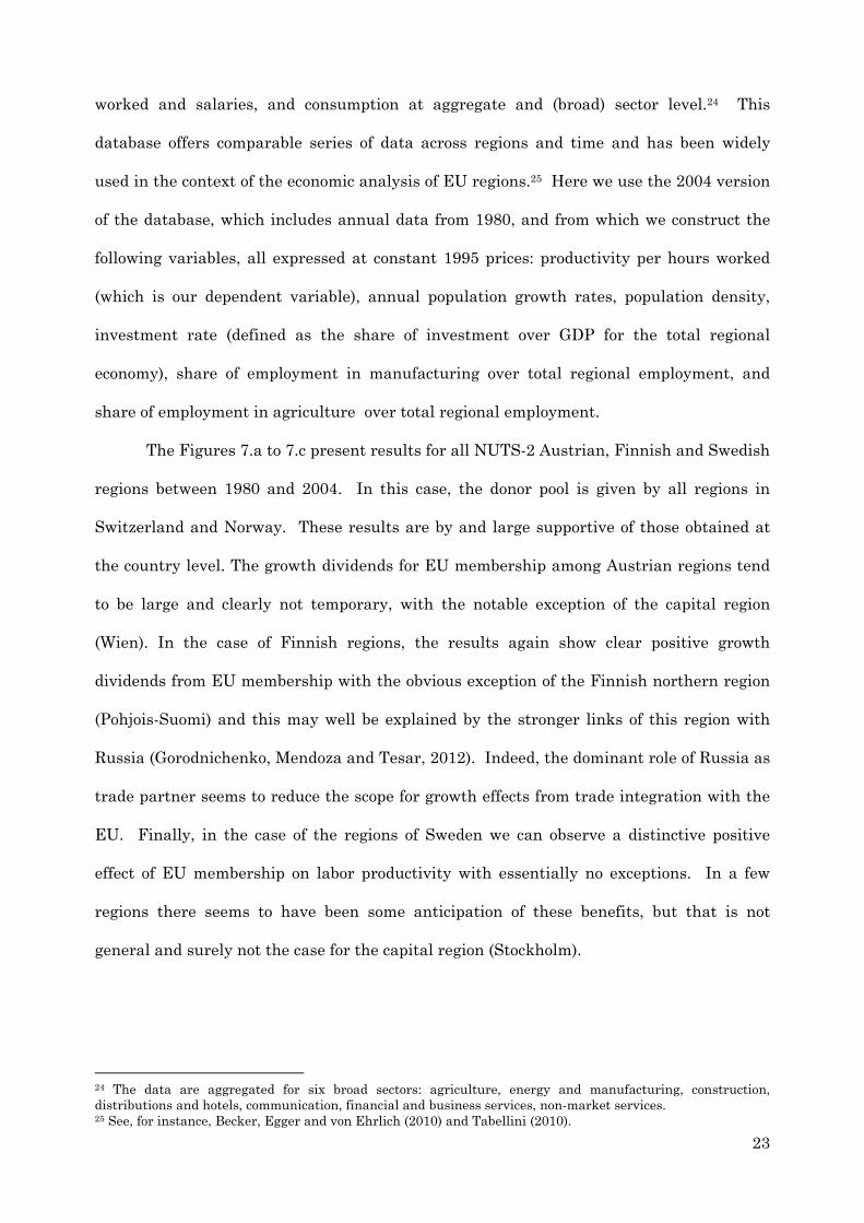
The Figures 7.a to 7.c present results for all NUTS-2 Austrian, Finnish and Swedish

regions between 1980 and 2004. In this case, the donor pool is given by all regions in

Switzerland and Norway. These results are by and large supportive of those obtained at

the country level. The growth dividends for EU membership among Austrian regions tend

to be large and clearly not temporary, with the notable exception of the capital region

(Wien). In the case of Finnish regions, the results again show clear positive growth

dividends from EU membership with the obvious exception of the Finnish northern region

(Pohjois-Suomi) and this may well be explained by the stronger links of this region with

Russia (Gorodnichenko, Mendoza and Tesar, 2012). Indeed, the dominant role of Russia as

trade partner seems to reduce the scope for growth effects from trade integration with the

EU. Finally, in the case of the regions of Sweden we can observe a distinctive positive

effect of EU membership on labor productivity with essentially no exceptions. In a few

regions there seems to have been some anticipation of these benefits, but that is not

general and surely not the case for the capital region (Stockholm).

                                                            24 The data are aggregated for six broad sectors: agriculture, energy and manufacturing, construction, distributions and hotels, communication, financial and business services, non-market services. 25 See, for instance, Becker, Egger and von Ehrlich (2010) and Tabellini (2010).

24  

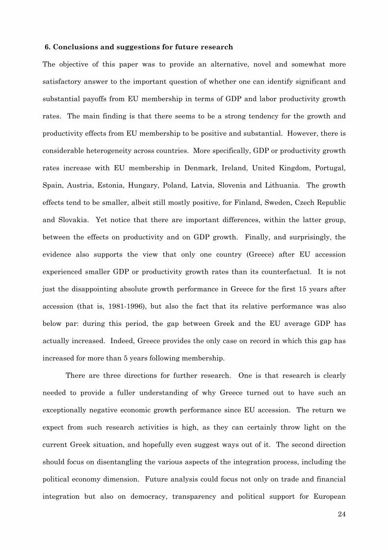
6. Conclusions and suggestions for future research

The objective of this paper was to provide an alternative, novel and somewhat more

satisfactory answer to the important question of whether one can identify significant and

substantial payoffs from EU membership in terms of GDP and labor productivity growth

rates. The main finding is that there seems to be a strong tendency for the growth and

productivity effects from EU membership to be positive and substantial. However, there is

considerable heterogeneity across countries. More specifically, GDP or productivity growth

rates increase with EU membership in Denmark, Ireland, United Kingdom, Portugal,

Spain, Austria, Estonia, Hungary, Poland, Latvia, Slovenia and Lithuania. The growth

effects tend to be smaller, albeit still mostly positive, for Finland, Sweden, Czech Republic

and Slovakia. Yet notice that there are important differences, within the latter group,

between the effects on productivity and on GDP growth. Finally, and surprisingly, the

evidence also supports the view that only one country (Greece) after EU accession

experienced smaller GDP or productivity growth rates than its counterfactual. It is not

just the disappointing absolute growth performance in Greece for the first 15 years after

accession (that is, 1981-1996), but also the fact that its relative performance was also

below par: during this period, the gap between Greek and the EU average GDP has

actually increased. Indeed, Greece provides the only case on record in which this gap has

increased for more than 5 years following membership.

There are three directions for further research. One is that research is clearly

needed to provide a fuller understanding of why Greece turned out to have such an

exceptionally negative economic growth performance since EU accession. The return we

expect from such research activities is high, as they can certainly throw light on the

current Greek situation, and hopefully even suggest ways out of it. The second direction

should focus on disentangling the various aspects of the integration process, including the

political economy dimension. Future analysis could focus not only on trade and financial

integration but also on democracy, transparency and political support for European

25  

integration. These issues appear particularly relevant in light of the tensions that arose

within the EU and especially within the Euro area as a result of the Great Recession. The

third and last area for further research regards the specific mechanisms and channels

through which EU membership seems able to support faster GDP and productivity growth

rates, as these mechanisms, and their effectiveness, may well have changed over time.

26  

References

Abadie, A., A. Diamond, and J. Hainmueller (2010), “Synthetic Control Methods for Comparative Case Studies: Estimating the Effect of California’s Tobacco Control Program,” Journal of American Statistical Association 105, 493–505. Abadie, A., A. Diamond, and J. Hainmueller (2012), “Comparative Politics and the Synthetic Control Method,” Harvard University, mimeo, July. Abadie, A., and J. Gardeazabal (2003), “The Economic Costs of Conflict: A Case Study of the Basque Country,” American Economic Review 93, 113–132. Acemoglu, D., (2009), Introduction to Modern Economic Growth, Princeton: Princeton University Press. Badinger, H. (2005), “Growth Effects of Economic Integration: Evidence from the EU Member States,” Review of World Economics 141: 50-78. Badinger, H. and F. Breuss (2010), “The Quantitative Effects of European Post-war Economic Integration,” in International Handbook on the Economics of Integration, volume III, Palgrave. Baldwin, R. (1989), “The Growth Effects of 1992,” Economic Policy 9: 247-81. Baldwin, R. (2008), “EU Institutional Reform: Evidence on Globalization and International Cooperation,” American Economic Review 98(2): 127–132. Baldwin, R.E., and E. Seghezza (1996), “Growth and European Integration: Towards an Empirical Assessment,” CEPR Discussion Paper no. 1393. Becker, S., P. Egger, and M. von Ehrlich (2010), “Going NUTS: The Effect of EU Structural Funds on Regional Performance”, Journal of Public Economics 94(9-10): 578-590. Berger, H. and V. Nitsch (2008), “Zooming Out: The Trade Effect of the Euro in Historical Perspective,” Journal of International Money and Finance 27: 1244–1260. Bertrand, M., E. Duflo and S. Mullainathan (2004), “How Much Should We Trust Differences-In-Differences Estimates?” Quarterly Journal of Economics 119(1): 249-275. Billmeier, A. and T. Nannicini (2012), “Assessing Economic Liberalization Episodes: A Synthetic Control Approach,” Review of Economics and Statistics, forthcoming. Boltho, A. and B. Eichengreen (2008), “The Economic Impact of European Integration,” CEPR Discussion Paper no. 6820. Bower, U. and A. Turrini (2010), “EU Accession: A Road to Fast-track Convergence?” Comparative Economic Studies 52: 181–205. Brou, D. and M. Ruta (2011), “Economic Integration, Political Integration or Both?” Journal of the European Economic Association 9(6):1143–1167. Campos, N. and Y. Kinoshita (2010), “Structural Reforms, Financial Liberalization and Foreign Direct Investment,” IMF Staff Papers 57(2): 326-365.

27  

Crafts, N. and G. Toniolo (2008), “European Economic Growth, 1950-2005: An Overview,” CEPR Discussion Paper No. 6863. Dorrucci, E., Firop, S., Fratzscher, M. and Mongelli, F. (2004). “The Link Between Institutional and Economic Integration: Insights for Latin America from the European Experience,” Open Economies Review, 15: 239-260. Eichengreen, B. (2007), The European Economy since 1945: Coordinated Capitalism and Beyond. Princeton, NJ: Princeton University Press. Elvert, J. and W. Kaiser (2004) (Editors) European Union Enlargement: A Comparative History, London: Routledge. Frankel, J. (2010), “The Estimated Trade Effects of the Euro: Why Are They Below Those from Historical Monetary Unions among Smaller Countries?” in A. Alesina and F. Giavazzi (eds.), Europe and the Euro, Chicago: University of Chicago Press. Friedrich, C., I. Schnabel and J. Zettelmeyer (2012), “Financial Integration and Growth: Why Is Emerging Europe Different?” Journal of International Economics, forthcoming. Gorodnichenko, Y., E. Mendoza and L. Tesar (2012), “The Finnish Great Depression: From Russia with Love,” American Economic Review 102(4): 1619-1643. Gordon, R. (2011), “Controversies about Work, Leisure, and Welfare in Europe and the United States,” in E. Phelps and H. Sinn (eds), Perspectives on the Performance of the Continental Economies, Cambridge: MIT Press: 343-386. Henrekson, M., J. Torstensson and R. Torstensson (1997), “Growth Effects of European Integration,” European Economic Review 41: 1537-1557. Henry, P. (2007), “Capital Account Liberalization: Theory, Evidence, and Speculation,” Journal of Economic Literature 45: 887–893. Imbens, G. and J. Wooldridge (2009), “Recent Developments in the Econometrics of Program Evaluation,” Journal of Economic Literature 47(1): 5–86. Jones, C. and P. Romer (2010), “The New Kaldor Facts: Ideas, Institutions, Population, and Human Capital” American Journal of Economics: Macroeconomics 2(1): 224–224. König, J. and R. Ohr (2012), ”The European Union: A Heterogeneous Community? Implications of an index measuring European integration,” Georg-August-Universität Göttingen, mimeo. Kutan, A. and T. Yigit (2007), “European Integration, Productivity Growth and Real Convergence,” European Economic Review 51: 1370–1395. Lee, W. (2011), “Comparative case studies of the effects of inflation targeting in emerging economies,” Oxford Economic Papers 63(2): 375–397. Martin, P., T. Mayer and M. Thoenig (2008), “Make Trade, Not War?” Review of Economic Studies 75: 865–900.

28  

Martin, P., T. Mayer and M. Thoenig (2012), “The Geography of Conflicts and Regional Trade Agreements,” American Economic Journal: Macroeconomics 4(4): 1-35. O’Mahony, M. and M. Timmer (2009), “Output, Input and Productivity Measures at the Industry Level: The EU KLEMS database,” The Economic Journal 119(June):374–403. Rivera-Batiz, L. A and P.M. Romer (1991), ”Economic Integration and Endogenous Growth,” Quarterly Journal of Economics 106(2): 531-555. Slaughter, M. (2001), “Trade liberalization and per capita income convergence: A difference-in-differences analysis,” Journal of International Economics 55: 203–228. Tabellini, G. (2010), “Culture and institutions: Economic development in the regions of Europe”, Journal of the European Economic Association 8(4): 677–716. Temin, P. (2002), “The Golden Age of European growth reconsidered,” European Review of Economic History 6: 3-22. Ventura, J. (2005), “A Global View of Economic Growth”, in Aghion, P. and S.N. Durlauf (eds.), Handbook of Economic Growth, North Holland, Elsevier Academic Press, Vol. 1B: 1419-1497. World Bank (2012), Golden Growth—Restoring the Luster of the European Economic Model, Washington.

29  

Table 1: Economic Growth in Europe and Around the World: 1820-2008

(Average annual compounded growth rates, GDP per capita, US$ 1990 Geary-Khamis PPP estimates)

Period Western Europe

Southern Europe

Eastern Europe

Former Soviet Union

United States

Japan East Asia Latin America

1820-1870 1.0 0.6 0.6 0.6 1.3 0.2 -0.1 0.0

1870-1913 1.3 1.0 1.4 1.0 1.8 1.4 0.8 1.8

1913-1950 0.8 0.4 0.6 1.7 1.6 0.9 -0.2 1.4

1950-1973 3.8 4.5 3.6 3.2 2.3 7.7 2.3 2.5

1973-1994 1.7 1.9 -0.2 -1.6 1.7 2.5 0.3 0.9

1994-2008 1.6 2.7 4.0 4.2 1.7 1.0 3.9 1.6

Note: Regional aggregates are population-weighted. Western Europe refers to Austria, Belgium, Denmark, Finland, France, West Germany, Italy, the Netherlands, Norway, Sweden, Switzerland, and the United Kingdom. Eastern Europe refers to Albania, Bulgaria, Czechoslovakia, Hungary, Poland, Romania, and Yugoslavia. Southern Europe refers to Greece, Ireland, Spain, and Turkey. After 1989, West Germany becomes Germany, and the data reflect the newly independent countries in Eastern Europe that emerge from Czechoslovakia and Yugoslavia.

Source: World Bank (2012)

30  

Notes on Figure 1 to 5: SYNTHETIC COUNTERFACTUAL RESULTS

There are two series plotted in each Figure. The one with a continuous line represents the actual per capita GDP or labor productivity levels of the country in question. The series with a dashed line plots the synthetic counterfactual results that purport to answer the following question:

What would have been the GDP (or productivity levels) of the country in question if it had NOT become an EU member in the year it did?

The synthetic counterfactuals are presented for each country in the last four EU enlargements: - Denmark, Ireland, and United Kingdom in the 1970s. - Greece, Spain and Portugal in the 1980s. - Austria, Finland and Sweden in the 1990s. - Eastern European countries in the 2000s.

Results are presented for two growth measures (per capita GDP and labor productivity). Others are available from the authors upon request. Results are presented for a donor pool of countries taken from Bower and Turrini (2010). The reported results are robust to dramatic changes in donor pool (from the whole world to selected EU neighbors); these are available from the authors upon request.

31  

Figure 1: Real GDP per capita in the Northern and Southern enlargements

1000

015

000

2000

025

000

3000

035

000

rgd

pch

1960 1980 2000 2020year

DNK synthetic DNK

1000

015

000

2000

025

000

3000

035

000

rgd

pch

1960 1980 2000 2020year

GBR synthetic GBR

010

000

2000

030

000

4000

0rg

dpc

h

1960 1980 2000 2020year

IRL synthetic IRL

1000

015

000

2000

025

000

3000

0rg

dpc

h

1970 1980 1990 2000 2010year

GRC synthetic GRC

1000

015

000

2000

025

000

3000

0rg

dpc

h

1970 1980 1990 2000 2010year

ESP synthetic ESP

5000

1000

015

000

2000

0rg

dpc

h

1970 1980 1990 2000 2010year

PRT synthetic PRT

2000

025

000

3000

035

000

4000

0rg

dpc

h

1980 1990 2000 2010year

AUT synthetic AUT

2000

025

000

3000

035

000

rgd

pch

1980 1990 2000 2010year

FIN synthetic FIN

2000

025

000

3000

035

000

4000

0rg

dpc

h

1980 1990 2000 2010year

SWE synthetic SWE

32  

Figure 2: Real GDP per capita in the Eastern enlargement

1400

016

000

1800

020

000

2200

024

000

rgd

pch

1990 1995 2000 2005 2010year

CZE synthetic CZE

5000

1000

015

000

2000

0rg

dpc

h

1990 1995 2000 2005 2010year

EST synthetic EST

1000

012

000

1400

016

000

1800

020

000

rgd

pch

1990 1995 2000 2005 2010year

HUN synthetic HUN

6000

8000

1000

012

000

1400

016

000

rgd

pch

1990 1995 2000 2005 2010year

LVA synthetic LVA

6000

8000

1000

012

000

1400

016

000

rgd

pch

1990 1995 2000 2005 2010year

LTU synthetic LTU

8000

1000

012

000

1400

016

000

rgd

pch

1990 1995 2000 2005 2010year

POL synthetic POL

1000

012

000

1400

016

000

1800

020

000

rgd

pch

1990 1995 2000 2005 2010year

SVK synthetic SVK

1500

020

000

2500

030

000

rgd

pch

1990 1995 2000 2005 2010year

SVN synthetic SVN

33  

Figure 3: Labor productivity in the Northern and Southern enlargement

2000

030

000

4000

050

000

6000

070

000

rgd

pwok

1960 1980 2000 2020year

DNK synthetic DNK

2000

030

000

4000

050

000

6000

070

000

rgd

pwok

1960 1980 2000 2020year

GBR synthetic GBR

2000

040

000

6000

080

000

rgd

pwok

1960 1980 2000 2020year

IRL synthetic IRL

3000

040

000

5000

060

000

7000

0rg

dpw

ok

1970 1980 1990 2000 2010year

GRC synthetic GRC

3000

040

000

5000

060

000

rgd

pwok

1970 1980 1990 2000 2010year

ESP synthetic ESP

2000

025

000

3000

035

000

4000

0rg

dpw

ok

1970 1980 1990 2000 2010year

PRT synthetic PRT

5000

055

000

6000

065

000

7000

075

000

rgd

pwok

1980 1990 2000 2010year

AUT synthetic AUT

3000

040

000

5000

060

000

7000

0rg

dpw

ok

1980 1990 2000 2010year

FIN synthetic FIN

4000

050

000

6000

070

000

rgd

pwok

1980 1990 2000 2010year

SWE synthetic SWE

34  

Figure 4: Labor productivity in the Eastern enlargement

3000

035

000

4000

045

000

5000

0rg

dpw

ok

1990 1995 2000 2005 2010year

CZE synthetic CZE

1500

020

000

2500

030

000

3500

0rg

dpw

ok

1990 1995 2000 2005 2010year

EST synthetic EST

2500

030

000

3500

040

000

4500

0rg

dpw

ok

1990 1995 2000 2005 2010year

HUN synthetic HUN

1000

015

000

2000

025

000

3000

0rg

dpw

ok

1990 1995 2000 2005 2010year

LVA synthetic LVA

1500

020

000

2500

030

000

3500

0rg

dpw

ok

1990 1995 2000 2005 2010year

LTU synthetic LTU

1500

020

000

2500

030

000

3500

0rg

dpw

ok

1990 1995 2000 2005 2010year

POL synthetic POL

2000

025

000

3000

035

000

4000

0rg

dpw

ok

1990 1995 2000 2005 2010year

SVK synthetic SVK

3000

035

000

4000

045

000

5000

055

000

rgd

pwok

1990 1995 2000 2005 2010year

SVN synthetic SVN

35  

Figure 5: Anticipation effects in real GDP per capita in the Eastern enlargement

1400

016

000

1800

020

000

2200

024

000

rgd

pch

1990 1995 2000 2005 2010year

CZE synthetic CZE

5000

1000

015

000

2000

0rg

dpc

h

1990 1995 2000 2005 2010year

EST synthetic EST

1000

012

000

1400

016

000

1800

0rg

dpc

h

1990 1995 2000 2005 2010year

HUN synthetic HUN

6000

8000

1000

012

000

1400

016

000

rgd

pch

1990 1995 2000 2005 2010year

LVA synthetic LVA

6000

8000

1000

012

000

1400

016

000

rgd

pch

1990 1995 2000 2005 2010year

LTU synthetic LTU

8000

1000

012

000

1400

016

000

rgd

pch

1990 1995 2000 2005 2010year

POL synthetic POL

1000

012

000

1400

016

000

1800

020

000

rgd

pch

1990 1995 2000 2005 2010year

SVK synthetic SVK

1500

020

000

2500

030

000

rgd

pch

1990 1995 2000 2005 2010year

SVN synthetic SVN

36  

Figure 6: Anticipation effects in labor productivity in the Eastern enlargement

3000

035

000

4000

045

000

5000

0rg

dpw

ok

1990 1995 2000 2005 2010year

CZE synthetic CZE

1500

020

000

2500

030

000

3500

0rg

dpw

ok

1990 1995 2000 2005 2010year

EST synthetic EST

2500

030

000

3500

040

000

4500

0rg

dpw

ok

1990 1995 2000 2005 2010year

HUN synthetic HUN

1000

015

000

2000

025

000

3000

0rg

dpw

ok

1990 1995 2000 2005 2010year

LVA synthetic LVA

1500

020

000

2500

030

000

3500

0rg

dpw

ok

1990 1995 2000 2005 2010year

LTU synthetic LTU

1500

020

000

2500

030

000

3500

0rg

dpw

ok

1990 1995 2000 2005 2010year

POL synthetic POL

2000

025

000

3000

035

000

4000

0rg

dpw

ok

1990 1995 2000 2005 2010year

SVK synthetic SVK

3000

035

000

4000

045

000

5000

055

000

rgd

pwok

1990 1995 2000 2005 2010year

SVN synthetic SVN

37  

Table 2: Differences-in-differences estimates of EU membership

Real GDP per capita Labor productivity

DID estimate and

std error

R-square and Number of obs

DID estimate and

std error

R-square and Number of obs

Denmark 4939 1389.870***

0.645 108

5235 2548.472**

0.625 108

United Kingdom 4882 1242.031***

0.575 108

12498 2302.802***

0.622 108

Ireland 6417 1693.316***

0.478 108

12641 3098.360***

0.607 108

Greece

-3680 1199.280***

0.523 78

-5055 2650.815*

0.385 78

Portugal

2969 818.513***

0.708 78

5786 1375.306***

0.699 78

Spain

2036 1163.037*

0.633 78

2725 1901.338

0.679 78

Austria 2500 1264.643*

0.718 58

5158 1863.316***

0.724 58

Sweden 182 1445.066

0.638 58

3462 2208.747

0.751 58

Finland 957 1507.296

0.620 58

4123 2707.401

0.681 58

Czech Republic -228 1315.601

0.444 32

-635 2588.259

0.432 32

Hungary 1514 773.860*

0.597 32

5944 1591.742***

0.686 32

Poland 2419 750.940***

0.640 32

6468 1653.858***

0.663 32

Estonia 2342 1416.446

0.496 32

4784 2628.393*

0.544 32

Latvia 3819 970.475***

0.575 32

3435 1989.282*

0.535 32

Lithuania 1368 1109.930

0.421 32

2993 2363.981

0.441 32

Slovakia 716 1305.509

0.480 32

-835 2737.253

0.468 32

Slovenia 1983 1417.173

0.568 32

3878 2288.965

0.574 32

Northern enlargement 1973

5412 1049.586***

0.478 324

10125 1767.457***

0.567 324

Southern enlargement 1981&1986

172 990.688

0.401 234

735 2760.823

0.221 234

Southern enlargement 1986

2503 1174.714***

0.432 156

4256 3241.477

0.225 156

Northern enlargement 1995

1213 966.225

0.561 174

4248 2062.294**

0.481 174

Eastern enlargement (1998-anticipation effect)

1742 1009.064*

0.176 256

3254 2064.973

0.183 256

NOTES: These results assess the statistical significance of the differences between the average difference pre-treatment (between the actual country and its synthetic) and the average difference post-treatment (between the actual country and its synthetic) estimated by the synthetic counterfactuals in Figures 1, 2, 5 and 6. Results are presented for each country and then for each enlargement and for GDP per capita and labor productivity series. The results are robust to other growth measures which are available upon request. Robust standard errors are reported. Inference: *** p<0.01; ** p<0.05; * p<0.1

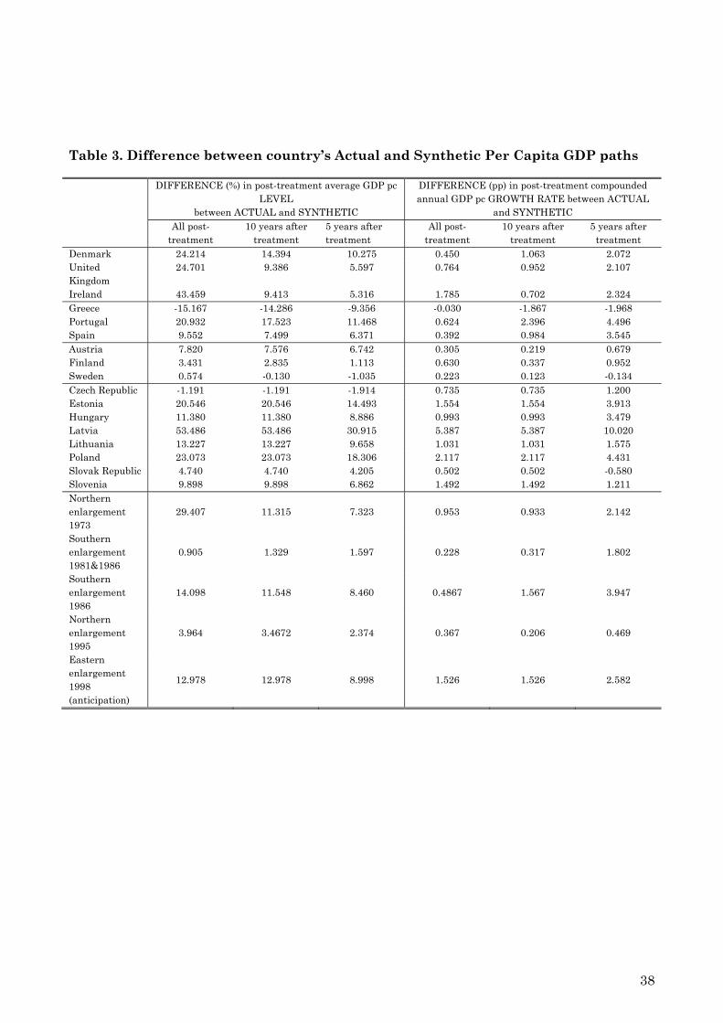
38  

Table 3. Difference between country’s Actual and Synthetic Per Capita GDP paths

DIFFERENCE (%) in post-treatment average GDP pc LEVEL

between ACTUAL and SYNTHETIC

DIFFERENCE (pp) in post-treatment compounded annual GDP pc GROWTH RATE between ACTUAL

and SYNTHETIC All post-

treatment 10 years after

treatment 5 years after treatment

All post-treatment

10 years after treatment

5 years after treatment

Denmark 24.214 14.394 10.275 0.450 1.063 2.072 United Kingdom

24.701 9.386 5.597 0.764 0.952 2.107

Ireland 43.459 9.413 5.316 1.785 0.702 2.324 Greece -15.167 -14.286 -9.356 -0.030 -1.867 -1.968 Portugal 20.932 17.523 11.468 0.624 2.396 4.496 Spain 9.552 7.499 6.371 0.392 0.984 3.545 Austria 7.820 7.576 6.742 0.305 0.219 0.679 Finland 3.431 2.835 1.113 0.630 0.337 0.952 Sweden 0.574 -0.130 -1.035 0.223 0.123 -0.134 Czech Republic -1.191 -1.191 -1.914 0.735 0.735 1.200 Estonia 20.546 20.546 14.493 1.554 1.554 3.913 Hungary 11.380 11.380 8.886 0.993 0.993 3.479 Latvia 53.486 53.486 30.915 5.387 5.387 10.020 Lithuania 13.227 13.227 9.658 1.031 1.031 1.575 Poland 23.073 23.073 18.306 2.117 2.117 4.431 Slovak Republic 4.740 4.740 4.205 0.502 0.502 -0.580 Slovenia 9.898 9.898 6.862 1.492 1.492 1.211 Northern enlargement 1973

29.407 11.315 7.323 0.953 0.933 2.142

Southern enlargement 1981&1986

0.905 1.329 1.597 0.228 0.317 1.802

Southern enlargement 1986

14.098 11.548 8.460 0.4867 1.567 3.947

Northern enlargement 1995

3.964 3.4672 2.374 0.367 0.206 0.469

Eastern enlargement 1998 (anticipation)

12.978 12.978 8.998 1.526 1.526 2.582

39  

Notes on Figure 6: SYNTHETIC COUNTERFACTUAL RESULTS USING REGIONAL DATA

Regional data for the 1995 enlargement: Austria, Finland and Sweden. The donor pool are regions from Norway and Switzerland. The dependent variable is the labor productivity per hour worked. The source of the regional data is Cambridge Econometrics.

40  

Figure 6.a: Regional labor productivity - Austria Burgenland Niederosterreich Wien

Karnten Steiermark Oberosterreich

Salzburg Tirol Vorarlberg

1520

25pr

1980 1985 1990 1995 2000 2005year

treated unit synthetic control unit

1618

2022

2426

pr

1980 1985 1990 1995 2000 2005year

treated unit synthetic control unit

2025

3035

pr

1980 1985 1990 1995 2000 2005year

treated unit synthetic control unit

1820

2224

26pr

1980 1985 1990 1995 2000 2005year

treated unit synthetic control unit

1618

2022

24pr

1980 1985 1990 1995 2000 2005year

treated unit synthetic control unit

1820

2224

2628

pr

1980 1985 1990 1995 2000 2005year

treated unit synthetic control unit

2022

2426

28pr

1980 1985 1990 1995 2000 2005year

treated unit synthetic control unit

2022

2426

pr

1980 1985 1990 1995 2000 2005year

treated unit synthetic control unit

2022

2426

28pr

1980 1985 1990 1995 2000 2005year

treated unit synthetic control unit

41  

Figure 6.b: Regional labor productivity - Finland

Itä-Suomi Etelä-Suomi Länsi-Suomi

Pohjois-Suomi

1618

2022

pr

1980 1985 1990 1995 2000 2005year

treated unit synthetic control unit

1520

2530

35pr

1980 1985 1990 1995 2000 2005year

treated unit synthetic control unit

1618

2022

2426

pr

1980 1985 1990 1995 2000 2005year

treated unit synthetic control unit

2224

2628

pr

1980 1985 1990 1995 2000 2005year

treated unit synthetic control unit

42  

Figure 6.c: Regional labor productivity - Sweden Stockholm Ostra Mellansverige Sydsverige

Norra Mellansverige Mellersta Norrland Ovre Norrland

Smaland med oarna Vastsverige

1520

2530

35pr

1980 1985 1990 1995 2000 2005year

treated unit synthetic control unit

1618

2022

2426

pr

1980 1985 1990 1995 2000 2005year

treated unit synthetic control unit

1520

2530

pr

1980 1985 1990 1995 2000 2005year

treated unit synthetic control unit

1820

2224

26pr

1980 1985 1990 1995 2000 2005year

treated unit synthetic control unit18

2022

2426

pr1980 1985 1990 1995 2000 2005

year

treated unit synthetic control unit

1820

2224

26pr

1980 1985 1990 1995 2000 2005year

treated unit synthetic control unit

1618

2022

24pr

1980 1985 1990 1995 2000 2005year

treated unit synthetic control unit

1618

2022

2426

pr

1980 1985 1990 1995 2000 2005year

treated unit synthetic control unit

43  

Appendix

44  

Table A.1: Unit weights and predictor balance – Real GDP per capita in the Northern and Southern enlargements DNK GBR IRL

Co_No Unit_Weight ARG 0 BRA 0 CHL 0 CHN 0 COL 0 EGY 0 JPN .14 KOR 0 MEX 0 NZL .86 PHL 0 THA 0 TUR 0

Treated Synthetic rgdpch 14128.42 13781.82 ki 18.5992 19.26247 openk 30.1045 23.64842 dens 113.4803 47.12548 popgr -.0734791 -.1410557 pop 4707.356 15871.74 agr 6.466325 11.53364 ind 31.92838 32.99036 ter 20.4622 19.18892 sec 93.00428 78.93301

Co_No Unit_Weight ARG .088 BRA 0 CHL 0 CHN 0 COL 0 EGY 0 JPN 0 KOR 0 MEX 0 NZL .912 PHL 0 THA 0 TUR 0

Treated Synthetic rgdpch 13913.92 13854.64 ki 14.05553 18.64536 openk 21.84542 25.20256 dens 225.9397 10.00904 popgr -.0290001 -.1532594 pop 53638.89 4239.138 agr 2.834722 12.45094 ind 41.51076 32.70868 ter 14.88064 18.92526 sec 75.38846 74.77053

Co_No Unit_Weight ARG .257 BRA 0 CHL 0 CHN 0 COL 0 EGY 0 JPN .203 KOR 0 MEX .015 NZL .24 PHL 0 THA 0 TUR .286

Treated Synthetic rgdpch 8184.698 8184.087 ki 18.71273 18.73474 openk 31.03721 14.54451 dens 42.19595 72.83208 popgr -.1567079 -.1624889 pop 2890.526 35512.44 agr 16.56953 20.26631 ind 34.49368 34.52512 ter 11.62112 13.68258 sec 74.38288 56.13163

GRC ESP PRT Co_No Unit_Weight ALB 0 ARG 0 AUS .281 BRA .132 CAN 0 CHE 0 CHL 0 CHN 0 COL 0 EGY 0 HKG 0 IDN 0 ISL 0 ISR 0 JPN .493 KOR 0 MAR 0 MEX 0 MYS 0 NZL 0 PHL 0 THA 0 TUN .093 TUR 0 URY 0

Treated Synthetic rgdpch 15438.97 15374.55 ki 30.68624 30.49525 openk 21.31609 21.45409 dens 70.92705 154.9721 popgr .001197 .0219185 pop 9140.592 73546.11 ter 15.91769 20.06139 sec 74.82954 75.50592

Co_No Unit_Weight ALB 0 ARG .198 AUS .522 BRA .19 CAN 0 CHE .012 CHL 0 CHN 0 COL 0 EGY 0 IDN 0 ISL 0 JPN .014 KOR .021 MAR .001 MEX .043 MYS 0 NZL 0 PHL 0 THA 0 TUN 0 TUR 0 URY 0

Treated Synthetic rgdpch 14801.19 14809.37 ki 22.62071 22.64224 openk 17.9698 18.22055 dens 72.85315 21.01268 popgr .0631041 .0632322 pop 36435.65 40125.24 agr 8.548183 8.564857 ind 37.5927 39.50187 ter 19.69868 19.71548 sec 76.33068 67.01273

Co_No Unit_Weight ALB 0 ARG 0 AUS 0 BRA 0 CAN 0 CHE .075 CHL 0 CHN 0 COL 0 EGY 0 IDN 0 ISL .189 JPN 0 KOR 0 MAR .1 MEX 0 MYS 0 NZL .042 PHL 0 THA 0 TUN .136 TUR .344 URY .114

Treated Synthetic rgdpch 9851.037 9863.569 ki 23.66904 26.33484 openk 30.26919 39.94156 dens 102.4411 42.89579 popgr .0176952 .0176214 pop 9521.294 18472.69 agr 21.99968 19.07358 ind 30.77487 30.7784 ter 10.54996 10.57261 sec 49.49542 50.64321

AUT FIN SWE Co_No Unit_Weight ALB 0 ARG 0 AUS .256 BRA 0 CAN 0 CHE .572 CHL .006 CHN 0 COL 0 EGY 0 IDN 0 ISL 0 JPN 0 KOR 0 MAR 0 MEX 0 MYS .166 NZL 0 PHL 0 THA 0 TUN 0 TUR 0 URY 0

Treated Synthetic rgdpch 25563.83 25599.76 ki 22.20473 26.49845 openk 60.13667 59.49917 dens 92.86038 103.5351 popgr .0313564 .1421614 pop 7680.184 10803.99 agr 3.86332 6.137594 ind 32.90471 34.16473 ter 29.14543 23.33576 sec 98.22047 98.11098

Co_No Unit_Weight ALB 0 ARG 0 AUS .002 BRA .118 CAN .313 CHE .042 CHL 0 CHN 0 COL 0 EGY 0 IDN 0 ISL .406 JPN 0 KOR 0 MAR 0 MEX 0 MYS 0 NZL .009 PHL 0 THA 0 TUN .107 TUR 0 URY .001

Treated Synthetic rgdpch 21584.77 21582.48 ki 24.05991 24.00462 openk 42.04161 53.45448 dens 16.19758 16.2057 popgr .0203774 .1459742 pop 4933.075 26483.03 agr 7.022083 8.844635 ind 34.50779 34.43856 ter 40.84733 40.50074 sec 108.2895 83.82644

Co_No Unit_Weight ALB 0 ARG 0 AUS 0 BRA 0 CAN .324 CHE .188 CHL .074 CHN 0 COL 0 EGY 0 IDN 0 ISL .267 JPN 0 KOR 0 MAR 0 MEX 0 MYS 0 NZL .147 PHL 0 THA 0 TUN 0 TUR 0 URY 0

Treated Synthetic rgdpch 24649.82 24651.62 ki 17.55956 21.22014 openk 50.63147 50.61927 dens 20.63541 35.73619 popgr .0273545 .140671 pop 8491.591 11418.76 agr 4.137151 6.492595 ind 30.5305 32.9409 ter 32.59514 46.08598 sec 93.11512 93.25807

45  

Figure A.1: Placebo cross-country – Real GDP per capita in the Northern and Southern enlargements

DNK GBR IRL

GRC ESP PRT

AUT FIN SWE

-10

000

-50

000

5000

1000

015

000

1960 1980 2000 2020_time

_rgdpch

-10

000

-50

000

5000

1000

0

1960 1980 2000 2020_time

_rgdpch

-10

000

010

000

2000

0

1960 1980 2000 2020_time

_rgdpch

-10

000

-50

000

5000

1000

0

1970 1980 1990 2000 2010_time

_rgdpch

-50

000

5000

1000

015

000

1970 1980 1990 2000 2010_time

_rgdpch

-50

000

5000

1000

0

1970 1980 1990 2000 2010_time

_rgdpch

-50

000

5000

1000

0

1980 1990 2000 2010_time

_rgdpch

-50

000

5000

1000

0

1980 1990 2000 2010_time

_rgdpch

-50

000

5000

1000

0

1980 1990 2000 2010_time

_rgdpch

46  

Table A.2: Unit weights and predictor balance – Labor productivity in the Northern and Southern enlargements DNK GBR IRL

Co_No Unit_Weight ARG 0 BRA 0 CHL 0 CHN 0 COL 0 EGY 0 JPN .355 KOR 0 MEX .084 NZL .561 PHL 0 THA 0 TUR 0

Treated Synthetic rgdpwok 30005.19 29968.94 ki 18.5992 20.95852 openk 30.1045 18.74878 dens 113.4803 105.0577 popgr -.0734791 -.1329159 pop 4707.356 39784.62 agr 6.466325 9.793382 ind 31.92838 35.33023 ter 20.4622 17.87791 sec 93.00428 76.37113

Co_No Unit_Weight ARG .278 BRA 0 CHL 0 CHN 0 COL 0 EGY 0 JPN .121 KOR 0 MEX 0 NZL .6 PHL 0 THA 0 TUR 0

Treated Synthetic rgdpwok 29986.85 29843.95 ki 14.05553 20.24261 openk 21.84542 20.90074 dens 225.9397 41.59006 popgr -.0290001 -.1543576 pop 53638.89 19411.06 agr 2.834722 11.06025 ind 41.51076 37.00394 ter 14.88064 18.00556 sec 75.38846 69.81651

Co_No Unit_Weight ARG 0 BRA 0 CHL 0 CHN 0 COL .335 EGY 0 JPN .398 KOR 0 MEX 0 NZL .267 PHL 0 THA 0 TUR 0

Treated Synthetic rgdpwok 20962.44 20924.27 ki 18.71273 21.77532 openk 31.03721 17.77406 dens 42.19595 117.6811 popgr -.1567079 -.1874131 pop 2890.526 45576.72 agr 16.56953 14.30623 ind 34.49368 34.68684 ter 11.62112 14.07285 sec 74.38288 64.18454

GRC ESP PRT Co_No Unit_Weight ALB 0 ARG 0 AUS 0 BRA .061 CAN 0 CHE .17 CHL 0 CHN 0 COL 0 EGY 0 HKG 0 IDN 0 ISL .572 ISR 0 JPN .197 KOR 0 MAR 0 MEX 0 MYS 0 NZL 0 PHL 0 THA 0 TUN 0 TUR 0 URY 0

Treated Synthetic rgdpwok 42784.13 42721.82 ki 30.68624 30.41041 openk 21.31609 44.85153 dens 70.92705 88.41666 popgr .001197 -.0081944 pop 9140.592 29742.9 ter 15.91769 15.90935 sec 74.82954 83.13898

Co_No Unit_Weight

ALB 0 ARG 0 AUS .413 BRA .23 CAN 0 CHE .134 CHL 0 CHN 0 COL 0 EGY 0 IDN 0 ISL 0 JPN .218 KOR 0 MAR 0 MEX .005 MYS 0 NZL 0 PHL 0 THA 0 TUN 0 TUR 0 URY 0

Treated Synthetic rgdpwok 39388.36 39268.66 ki 22.62071 24.61626 openk 17.9698 20.35542 dens 72.85315 92.88469 popgr .0631041 .0571259 pop 36435.65 58543.7 agr 8.548183 6.903183 ind 37.5927 38.58924 ter 19.69868 19.70236 sec 76.33068 76.33312

Co_No Unit_Weight ALB .003 ARG 0 AUS 0 BRA 0 CAN 0 CHE 0 CHL 0 CHN 0 COL .373 EGY 0 IDN 0 ISL .232 JPN 0 KOR 0 MAR 0 MEX 0 MYS 0 NZL .062 PHL 0 THA 0 TUN .064 TUR .267 URY 0

Treated Synthetic rgdpwok 22494.05 22527.2 ki 23.66904 23.17229 openk 30.26919 33.27717 dens 102.4411 27.16638 popgr .0176952 .0314353 pop 9521.294 21614.83 agr 21.99968 21.11588 ind 30.77487 30.79941 ter 10.54996 10.56679 sec 49.49542 49.59341

AUT FIN SWE Co_No Unit_Weight ALB 0 ARG 0 AUS .112 BRA 0 CAN .274 CHE .614 CHL 0 CHN 0 COL 0 EGY 0 IDN 0 ISL 0 JPN 0 KOR 0 MAR 0 MEX 0 MYS 0 NZL 0 PHL 0 THA 0 TUN 0 TUR 0 URY 0

Treated Synthetic rgdpwok 56832.47 55706.88 ki 22.20473 23.62397 openk 60.13667 51.05631 dens 92.86038 102.3621 popgr .0313564 .1174451 pop 7680.184 13266.7 agr 3.86332 3.337138 ind 32.90471 32.78999 ter 29.14543 42.04317 sec 98.22047 100.4226

Co_No Unit_Weight ALB 0 ARG 0 AUS 0 BRA 0 CAN .244 CHE 0 CHL 0 CHN 0 COL 0 EGY 0 IDN 0 ISL .462 JPN 0 KOR .17 MAR 0 MEX 0 MYS 0 NZL 0 PHL 0 THA 0 TUN 0 TUR 0 URY .123

Treated Synthetic rgdpwok 41699.93 41657.21 ki 24.05991 24.05948 openk 42.04161 48.38746 dens 16.19758 75.48382 popgr .0203774 .1458365 pop 4933.075 14088.89 agr 7.022083 9.476161 ind 34.50779 34.45906 ter 40.84733 40.76466 sec 108.2895 91.4924

Co_No Unit_Weight ALB 0 ARG 0 AUS 0 BRA 0 CAN .9 CHE 0 CHL 0 CHN 0 COL 0 EGY .059 IDN 0 ISL 0 JPN 0 KOR 0 MAR 0 MEX 0 MYS .042 NZL 0 PHL 0 THA 0 TUN 0 TUR 0 URY 0

Treated Synthetic rgdpwok 47167.41 47203.16 ki 17.55956 18.81346 openk 50.63147 50.66183 dens 20.63541 7.94606 popgr .0273545 .1679103 pop 8491.591 27842.08 agr 4.137151 4.846499 ind 30.5305 33.00149 ter 32.59514 80.07969 sec 93.11512 93.60544

47  

Figure A.2: Placebo cross-country – Labor productivity in the Northern and Southern enlargements

DNK GBR IRL

GRC ESP PRT

AUT FIN SWE

-10

000

010

000

2000

030

000

4000

0

1960 1980 2000 2020_time

_rgdpwok

-10

000

010

000

2000

030

000

4000

0

1960 1980 2000 2020_time

_rgdpwok

-10

000

010

000

2000

030

000

4000

0

1960 1980 2000 2020_time

_rgdpwok

-30

000

-20

000

-10

000

010

000

2000

0

1970 1980 1990 2000 2010_time

_rgdpwok

-20

000

-10

000

010

000

1970 1980 1990 2000 2010_time

_rgdpwok

-50

000

5000

1000

015

000

1970 1980 1990 2000 2010_time

_rgdpwok

-10

000

-50

000

5000

1000

0

1980 1990 2000 2010_time

_rgdpwok

-10

000

010

000

2000

0

1980 1990 2000 2010_time

_rgdpwok

-40

00-2

000

020

0040

0060

00

1980 1990 2000 2010_time

_rgdpwok

48  

Table A.3: Unit weights and predictor balance –Real GDP per capita in the Eastern enlargement (1998 anticipation)

CZE EST HUN Co_No Unit_W ALB 0 ARG 0 AUS 0 BRA 0 CAN 0 CHE 0 CHL 0 CHN 0 COL 0 EGY 0 HKG 0 HRV .631 IDN 0 ISL .171 ISR 0

Co_No Unit_W JPN .175 KOR 0 MAR 0 MEX 0 MKD 0 MYS 0 NZL 0 PHL 0 RUS 0 THA 0 TUN 0 TUR 0 UKR 0 URY .023

Treated Synthetic rgdpch 15261.36 15267.26 ki 22.16795 22.16668 openk 69.43389 70.97353 dens 133.5837 113.0011 popgr .0486624 .0742206 pop 10318.59 24877.22 ter 20.3791 30.25677 sec 91.11272 88.80191

Co_No Unit_W ALB 0 ARG 0 AUS 0 BRA 0 CAN 0 CHE 0 CHL 0 CHN 0 COL 0 EGY 0 HKG 0 HRV .878 IDN 0 ISL 0 ISR 0

Co_No Unit_W JPN 0 KOR 0 MAR 0 MEX 0 MKD 0 MYS .047 NZL 0 PHL 0 RUS 0 THA 0 TUN .008 TUR 0 UKR .066 URY 0

Treated Synthetic rgdpch 7783.545 7776.776 ki 21.63741 21.59448 openk 105.5148 92.46768 dens 34.00993 81.56834 popgr .152569 .092854 pop 1449.33 8340.764 ter 31.31793 26.83056 sec 96.84887 81.11214

Co_No Unit_W ALB 0 ARG 0 AUS 0 BRA 0 CAN 0 CHE 0 CHL 0 CHN 0 COL 0 EGY .042 HKG .01 HRV 0 IDN 0 ISL .197 ISR 0

Co_No Unit_W JPN 0 KOR 0 MAR 0 MEX .218 MKD .53 MYS 0 NZL 0 PHL 0 RUS 0 THA 0 TUN 0 TUR 0 UKR 0 URY .002

Treated Synthetic rgdpch 11035.94 11001.41 ki 17.06667 18.58144 openk 57.38999 67.41381 dens 114.9309 113.9884 popgr -.0001189 .1747698 pop 10291.17 23878.41 ter 21.47465 21.43687 sec 92.37348 78.00207

LVA LTU POL Co_No Unit_W ALB 0 ARG 0 AUS 0 BRA 0 CAN 0 CHE 0 CHL 0 CHN 0 COL 0 EGY .341 HKG 0 HRV 0 IDN 0 ISL 0 ISR 0

Co_No Unit_W JPN 0 KOR 0 MAR 0 MEX 0 MKD 0 MYS 0 NZL 0 PHL 0 RUS 0 THA 0 TUN 0 TUR 0 UKR 0 URY .659

Treated Synthetic

rgdpch 6377.258 6381.024 ki 12.20334 16.21778 openk 82.46302 50.10215 dens 40.06805 33.38711 popgr .0163368 .2677545 pop 2494.698 22217.19 ter 26.22805 31.74279 sec 88.50974 78.27632

Co_No Unit_W ALB 0 ARG 0 AUS 0 BRA 0 CAN .013 CHE 0 CHL 0 CHN 0 COL 0 EGY 0 HKG .046 HRV .515 IDN 0 ISL 0 ISR 0

Co_No Unit_W JPN 0 KOR 0 MAR 0 MEX 0 MKD .005 MYS 0 NZL 0 PHL 0 RUS 0 THA 0 TUN 0 TUR 0 UKR .421 URY 0

Treated Synthetic rgdpch 7586.694 7587.52 ki 10.7057 20.64397 openk 91.09633 90.97001 dens 57.8992 354.0716 popgr .1377906 .1040714 pop 3674.981 24539.4 ter 27.95088 33.58612 sec 86.00709 85.989

Co_No Unit_W ALB 0 ARG 0 AUS .11 BRA 0 CAN 0 CHE 0 CHL 0 CHN 0 COL 0 EGY .283 HKG 0 HRV 0 IDN 0 ISL 0 ISR 0

Co_No Unit_W JPN 0 KOR 0 MAR 0 MEX 0 MKD 0 MYS 0 NZL 0 PHL 0 RUS 0 THA 0 TUN 0 TUR 0 UKR 0 URY .607

Treated Synthetic rgdpch 8928.349 8942.925 ki 15.95067 16.86188 openk 42.28706 48.34186 dens 126.731 29.07228 popgr .2625728 .2626474 pop 38580.3 20607.13 ter 31.61196 35.97875 sec 96.92753 85.49217

SVK SVN Co_No Unit_W ALB 0 ARG 0 AUS .128 BRA .051 CAN 0 CHE 0 CHL 0 CHN 0 COL 0 EGY 0 HKG .008 HRV .669 IDN 0 ISL 0 ISR 0

Co_No Unit_W JPN 0 KOR 0 MAR 0 MEX 0 MKD 0 MYS .144 NZL 0 PHL 0 RUS 0 THA 0 TUN 0 TUR 0 UKR 0 URY 0

Treated Synthetic rgdpch 10898.34 10911.87 ki 21.37569 24.15714 openk 92.13366 92.11543 dens 111.3941 113.0656 popgr .2009542 .2011651 pop 5357.327 16623.31 ter 18.78215 29.28024 sec 89.27523 86.71877

Co_No Unit_W ALB 0 ARG 0 AUS .165 BRA 0 CAN .176 CHE 0 CHL 0 CHN 0 COL 0 EGY 0 HKG .008 HRV .465 IDN 0 ISL 0 ISR 0

Co_No Unit_W JPN 0 KOR 0 MAR 0 MEX 0 MKD 0 MYS .187 NZL 0 PHL 0 RUS 0 THA 0 TUN 0 TUR 0 UKR 0 URY 0

Treated Synthetic rgdpch 15292.52 15310.3 ki 23.12446 24.83614 openk 92.48478 92.59097 dens 98.76509 98.66479 popgr .210008 .2544466 pop 2004.566 14129.23 ter 30.99486 41.99612 sec 90.91187 90.9946

49  

Figure A.3: Placebo cross-country – Real GDP per capita in the Eastern enlargement (1998 anticipation)

CZE EST HUN

LVA LTU POL

SVK SVN

-50

000

5000

1990 1995 2000 2005 2010_time

_rgdpch

-20

000

2000

4000

6000

1990 1995 2000 2005 2010_time

_rgdpch

-20

000

2000

4000

6000

1990 1995 2000 2005 2010_time

_rgdpch

-20

000

2000

4000

6000

8000

1990 1995 2000 2005 2010_time

_rgdpch

-20

000

2000

4000

6000

1990 1995 2000 2005 2010_time

_rgdpch

-20

000

2000

4000

1990 1995 2000 2005 2010_time

_rgdpch

-20

000

2000

4000

6000

1990 1995 2000 2005 2010_time

_rgdpch

-20

000

2000

4000

6000

1990 1995 2000 2005 2010_time

_rgdpch

50  

Table A.4: Unit weights and predictor balance – Labor productivity in the Eastern enlargement (1998 anticipation)

CZE EST HUN Co_No Unit_W ALB 0 ARG 0 AUS 0 BRA 0 CAN 0 CHE 0 CHL 0 CHN 0 COL 0 EGY 0 HKG .004 HRV .577 IDN 0 ISL .172 ISR 0

Co_No Unit_W JPN .18 KOR 0 MAR 0 MEX 0 MKD 0 MYS 0 NZL 0 PHL 0 RUS 0 THA 0 TUN 0 TUR 0 UKR 0 URY .067

Treated Synthetic rgdpwok 30558.09 30550.2 ki 22.16795 22.16745 openk 69.43389 69.49417 dens 133.5837 134.9004 popgr .0486624 .0768296 pop 10318.59 25425.71 ter 20.3791 30.41847 sec 91.11272 88.93057

Co_No Unit_W ALB 0 ARG 0 AUS 0 BRA 0 CAN 0 CHE 0 CHL 0 CHN 0 COL 0 EGY 0 HKG 0 HRV .765 IDN 0 ISL 0 ISR 0

Co_No Unit_W JPN 0 KOR 0 MAR 0 MEX 0 MKD 0 MYS .05 NZL 0 PHL .185 RUS 0 THA 0 TUN 0 TUR 0 UKR 0 URY 0

Treated Synthetic rgdpwok 15708.13 15709.98 ki 21.63741 22.04206 openk 105.5148 96.4155 dens 34.00993 109.1165 popgr .152569 .2145071 pop 1449.33 17889.37 ter 31.31793 26.27984 sec 96.84887 79.50583

Co_No Unit_W ALB 0 ARG .001 AUS .11 BRA .002 CAN .146 CHE 0 CHL .001 CHN 0 COL .001 EGY .024 HKG 0 HRV .001 IDN 0 ISL .004 ISR 0

Co_No Unit_W JPN 0 KOR 0 MAR 0 MEX .002 MKD .006 MYS 0 NZL 0 PHL .001 RUS .001 THA 0 TUN 0 TUR .001 UKR .002 URY .694

Treated Synthetic rgdpwok 27574.6 27495.06 ki 17.06667 18.07437 openk 57.38999 49.49066 dens 114.9309 16.23989 popgr -.0001189 .1543053 pop 10291.17 10915.75 ter 21.47465 42.72911 sec 92.37348 91.78547

LVA LTU POL Co_No Unit_W ALB 0 ARG 0 AUS 0 BRA 0 CAN 0 CHE 0 CHL 0 CHN 0 COL 0 EGY 0 HKG 0 HRV .562 IDN 0 ISL 0 ISR 0

Co_No Unit_W JPN 0 KOR 0 MAR .438 MEX 0 MKD 0 MYS 0 NZL 0 PHL 0 RUS 0 THA 0 TUN 0 TUR 0 UKR 0 URY 0

Treated Synthetic rgdpwok 13127.59 13142.47 ki 12.20334 23.59068 openk 82.46302 73.76906 dens 40.06805 72.68391 popgr .0163368 .0648894 pop 2494.698 13967.11 ter 26.22805 19.88665 sec 88.50974 62.66599

Co_No Unit_W ALB 0 ARG 0 AUS .005 BRA 0 CAN 0 CHE 0 CHL 0 CHN 0 COL 0 EGY 0 HKG .029 HRV .556 IDN 0 ISL 0 ISR 0

Co_No Unit_W JPN 0 KOR 0 MAR 0 MEX 0 MKD 0 MYS 0 NZL 0 PHL 0 RUS 0 THA 0 TUN 0 TUR 0 UKR .41 URY 0

Treated Synthetic rgdpwok 15402.28 15427.88 ki 10.7057 20.40715 openk 91.09633 88.30643 dens 57.8992 254.8456 popgr .1377906 .0949265 pop 3674.981 23748.86 ter 27.95088 32.98372 sec 86.00709 85.9614

Co_No Unit_W ALB 0 ARG 0 AUS .102 BRA .001 CAN 0 CHE 0 CHL 0 CHN 0 COL 0 EGY .289 HKG 0 HRV 0 IDN 0 ISL 0 ISR 0

Co_No Unit_W JPN 0 KOR 0 MAR 0 MEX 0 MKD 0 MYS 0 NZL 0 PHL 0 RUS 0 THA 0 TUN 0 TUR 0 UKR 0 URY .608

Treated Synthetic rgdpwok 19815.68 19834.82 ki 15.95067 16.80936 openk 42.28706 48.44448 dens 126.731 29.4652 popgr .2625728 .2644932 pop 38580.3 20984.26 ter 31.61196 35.66494 sec 96.92753 84.96109

SVK SVN Co_No Unit_W ALB 0 ARG 0 AUS .128 BRA 0 CAN 0 CHE 0 CHL 0 CHN 0 COL 0 EGY 0 HKG .007 HRV .801 IDN 0 ISL 0 ISR 0

Co_No Unit_W JPN 0 KOR 0 MAR 0 MEX 0 MKD 0 MYS .064 NZL 0 PHL 0 RUS 0 THA 0 TUN 0 TUR 0 UKR 0 URY 0

Treated Synthetic rgdpwok 23441.75 23471.65 ki 21.37569 22.22432 openk 92.13366 89.00794 dens 111.3941 111.9551 popgr .2009542 .1312204 pop 5357.327 7238.56 ter 18.78215 31.38228 sec 89.27523 87.94202

Co_No Unit_W ALB 0 ARG 0 AUS .08 BRA 0 CAN .06 CHE 0 CHL 0 CHN 0 COL 0 EGY 0 HKG .01 HRV .071 IDN 0 ISL .295 ISR 0

Co_No Unit_W JPN 0 KOR 0 MAR 0 MEX 0 MKD .344 MYS .14 NZL 0 PHL 0 RUS 0 THA 0 TUN 0 TUR 0 UKR 0 URY 0

Treated Synthetic rgdpwok 32639.39 32633.84 ki 23.12446 23.14465 openk 92.48478 85.28437 dens 98.76509 101.9445 popgr .210008 .2102692 pop 2004.566 7199.799 ter 30.99486 30.9654 sec 90.91187 88.97266

51  

Figure A.4: Placebo cross-country – Labor productivity in the Eastern enlargement (1998 anticipation)

CZE EST HUN

LVA LTU POL

SVK SVN

-50

000

5000

1000

015

000

1990 1995 2000 2005 2010_time

_rgdpwok

-50

000

5000

1000

015

000

1990 1995 2000 2005 2010_time

_rgdpwok

-50

000

5000

1000

015

000

1990 1995 2000 2005 2010_time

_rgdpwok

-50

000

5000

1000

015

000

1990 1995 2000 2005 2010_time

_rgdpwok

-50

000

5000

1000

015

000

1990 1995 2000 2005 2010_time

_rgdpwok

-50

000

5000

1000

0

1990 1995 2000 2005 2010_time

_rgdpwok

-50

000

5000

1000

015

000

1990 1995 2000 2005 2010_time

_rgdpwok

-50

000

5000

1000

015

000

1990 1995 2000 2005 2010_time

_rgdpwok