Economic Development, Mobility and Political Discontent: An

Experimental Test of Tocqueville's Thesis in Pakistan∗

Andrew Healy† Katrina Kosec‡ Cecilia Hyunjung Mo§

June 13, 2016

Abstract

We consider the thesis of Alexis de Tocqueville (1856) that economic development and increased mobility may generate political discontent not present in more stagnant economies. For many citizens, as they become aware of the potential for improvement, aspirations may increase faster than living standards. Expanded opportunity may then paradoxically result in dissatisfaction with government rather than greater confidence. We develop a formal model to capture Toc- queville’s (1856) verbal theory and test its predictions using a 2012–2013 face-to-face survey ex- periment conducted in Pakistan. The experiment utilizes established treatments to manipulate either a participant’s perceptions of her own economic well-being, her perceptions of society- wide mobility, or both. As predicted by the theory, political discontent often rises the most when declining personal well-being coincides with high mobility. The results thus identify the conditions under which expanded economic opportunity can lead to political unrest.

1-2016 – Elections and Electoral Rules

∗We thank the dedicated team at Innovative Development Strategies (IDS), who in collaboration with the Inter-

national Food Policy Research Institute (IFPRI), carried out the extensive data collection activities for our Pakistan Rural Household Panel Survey (RHPS). We also thank Alemayehu Seyoum Taffesse and Tanguy Bernard for pro- viding us with the Aspirations module from the IFPRI Ethiopia Rural Household Survey, which helped inform the Aspirations module in the Pakistan RHPS. We gratefully acknowledge insightful comments and guidance from Adam Meirowitz, Emily Nacol, Danielle Resnick, Alan Wiseman, and Elizabeth Zechmeister, as well as the discussants and participants at the 2016 annual meeting of the Behavioral Models of Politics at University of Pittsburgh, Midwest Political Science Association, and the Southern Political Science Association. All remaining errors are our own.

†Andrew Healy: Professor of Economics, Loyola Marymount University, One LMU Drive, Room 4229, Los Angeles, CA 90045 (ahealy@lmu.edu).

‡Katrina Kosec: Research Fellow, International Food Policy Research Institute, Development Strategy and Gov- ernance Division, 2033 K Street, NW, Washington, D.C. 20006 (k.kosec@cgiar.org).

§Cecilia Hyunjung Mo: Assistant Professor of Political Science, Vanderbilt University, PMB 0505, 230 Appleton

Place, Nashville, TN 37203 (cecilia.h.mo@vanderbilt.edu); W. Glenn Campbell and Rita Ricardo-Campbell National Fellow and Robert Eckles Swain National Fellow, Hoover Institution, Stanford University, 434 Galvez Mall, Stanford, CA 94305.

Economic Development, Mobility and Political Discontent: An

Experimental Test of Tocqueville’s Thesis in Pakistan∗

Andrew Healy† Katrina Kosec‡ Cecilia Hyunjung Mo§

June 13, 2016

Abstract

We consider the thesis of Alexis de Tocqueville (1856) that economic development and increasedmobility may generate political discontent not present in more stagnant economies. For manycitizens, as they become aware of the potential for improvement, aspirations may increase fasterthan living standards. Expanded opportunity may then paradoxically result in dissatisfactionwith government rather than greater confidence. We develop a formal model to capture Toc-queville’s (1856) verbal theory and test its predictions using a 2012–2013 face-to-face survey ex-periment conducted in Pakistan. The experiment utilizes established treatments to manipulateeither a participant’s perceptions of her own economic well-being, her perceptions of society-wide mobility, or both. As predicted by the theory, political discontent often rises the mostwhen declining personal well-being coincides with high mobility. The results thus identify theconditions under which expanded economic opportunity can lead to political unrest.

∗We thank the dedicated team at Innovative Development Strategies (IDS), who in collaboration with the Inter-national Food Policy Research Institute (IFPRI), carried out the extensive data collection activities for our PakistanRural Household Panel Survey (RHPS). We also thank Alemayehu Seyoum Taffesse and Tanguy Bernard for pro-viding us with the Aspirations module from the IFPRI Ethiopia Rural Household Survey, which helped inform theAspirations module in the Pakistan RHPS. We gratefully acknowledge insightful comments and guidance from AdamMeirowitz, Emily Nacol, Danielle Resnick, Alan Wiseman, and Elizabeth Zechmeister, as well as the discussants andparticipants at the 2016 annual meeting of the Behavioral Models of Politics at University of Pittsburgh, MidwestPolitical Science Association, and the Southern Political Science Association. All remaining errors are our own.†Andrew Healy: Professor of Economics, Loyola Marymount University, One LMU Drive, Room 4229, Los Angeles,

CA 90045 (ahealy@lmu.edu).‡Katrina Kosec: Research Fellow, International Food Policy Research Institute, Development Strategy and Gov-

ernance Division, 2033 K Street, NW, Washington, D.C. 20006 (k.kosec@cgiar.org).§Cecilia Hyunjung Mo: Assistant Professor of Political Science, Vanderbilt University, PMB 0505, 230 Appleton

Place, Nashville, TN 37203 (cecilia.h.mo@vanderbilt.edu); W. Glenn Campbell and Rita Ricardo-Campbell NationalFellow and Robert Eckles Swain National Fellow, Hoover Institution, Stanford University, 434 Galvez Mall, Stanford,CA 94305.

Introduction

Intuitively, economic development should increase confidence in government. Development re-

duces poverty, and governments should be rewarded for doing so. Classic economic voting theory,

which articulates that citizens reward the incumbent for good times and punish the incumbent

for bad, has received substantial empirical support (Lewis-Beck and Nadeau 2011). But economic

development has at times coincided with exactly the opposite outcome: dissatisfaction with gov-

ernment. Modern day China is an example; the number of protest incidents in China increased

only modestly from 1997 to 1999, when economic growth was relatively slow. As China’s econ-

omy began booming again in 2001, the number and scale of protests rose sharply (Keidel 2005).

The French Revolution, which started in the most prosperous parts of France, provides another

case. As Tocqueville observes, “the parts of France that were to become the principal center of

that revolution were precisely those where progress was most evident” (Tocqueville 1856, 156). To

reconcile this paradox, he raises the possibility that the arrival of some limited opportunity may

throw into sharp relief the gap between what citizens feel they should have and what they actually

have—a concept that has been termed the “aspirations gap” (Ray 2006). Here, we formally capture

and experimentally test Tocqueville’s verbal theory that economic development can coincide with

political unrest.

This phenomenon has been dubbed the “Tocqueville Effect”; it conveys “the idea that subjective

discontent (and hence the likelihood of revolution or rebellion) and objective grounds for discontent

can be inversely related to each other” (Goldhammer and Elster 2011, 162-163). The theory posits

that radical change often arises not during economic hardship, but rather when conditions increase

expectations. For those individuals who develop aspirations that are not met, their confidence

in government may actually decrease when mobility increases. Other researchers have taken an

interest in exploring the conundrum that economic mobility does not necessarily translate to greater

confidence in government. More recently, Acemoglu, Egorov, and Sonin (2015) present a formal

model capturing additional conditions under which economic mobility and political stability may

conflict. They describe how high mobility can decrease stability if the median voter expects to move

up the income distribution and thus prefers to decrease the voice given to poorer social groups.1

1When the mean and median policy preferences are close, they argue that “not only is democracy stable (meaningthat the median voter would not wish to undermine democracy), but it also becomes more stable as social mobility

1

Political theorists have often referred to American democracy to illustrate how economic op-

portunity can increase the strength of political institutions. Tocqueville (1835) famously argued

in Democracy in America that mobility increased political stability, in contrast to his later work.

Lipset (1960), Moore (1966), and Blau and Duncan (1967), among others, make similar points. For

example, Blau and Duncan (1967) conclude that “the stability of American democracy is undoubt-

edly related to the superior chances of upward mobility in this country” (439). In the American

case, however, mobility has tended to increase political stability because economic conditions have

kept pace with increased expectations; this contrasts with many other cases, like those of France

on the eve of the revolution. These counterexamples point to the fact that economic opportunity

does not necessarily increase political stability.

Here, we develop a formal model with two testable propositions capturing the logic of the

“Tocqueville Effect.” We then test these propositions using an experiment which we carried out

in Pakistan. The experiment utilizes standard treatments to manipulate either a participant’s

perceptions of her own economic well-being or her perceptions of possibilities for upward mobility

within Pakistan, employing a 2 (poverty prime, no poverty prime) × 2 (mobility prime, no mobility

prime) research design. This design exogenously manipulates the perceived gap between where

participants feel they are presently and where they aspire to be in terms of economic and social

status—i.e. their aspirations gap. We then assess how these primes individually and jointly affect

confidence in government. We find substantial empirical support for the model’s predictions.

While the implications of our model apply more broadly, Pakistan is an interesting context

for several reasons. First, it is a middle-income country with the world’s sixth-largest population

(Central Intelligence Agency 2015), helping lend Pakistan a great degree of geopolitical signifi-

cance. Second, Pakistan is a young democracy, which has made genuine democratic progress over

the last few years.2 Third, Pakistan has a fragile security situation. A number of militant or-

ganizations operate in Pakistan, threatening further domestic progress and international stability

(Lamb 2008; Ghani and Lockhart 2009; Blair, Neumann, and Olson 2014). Understanding what

drives support for government is critical since opposition to government may lead to support for

increases. Conversely, when the mean and median are far apart, greater social mobility reduces the stability ofdemocracy” (30).

2In 2013, the country saw its first successful transition from one democratically elected government to another,and additionally passed a landmark right-to-information law that provides citizens with access to public documents.Source: http://tribune.com.pk/story/564305/right-to-information-act-2013/.

2

extremist groups (Patrick 2010; Felbab-Brown 2010). Lessons from Pakistan are thus likely to be

useful for understanding peace and stability in many fragile and failed state contexts. Finally,

Pakistan is a relatively mobile country; the OECD (2012) found that Pakistan has the same level

of inter-generational mobility found in Switzerland, and higher mobility than many of the 22 other

countries studied, including the United States, the United Kingdom, Italy, and China.3 Pakistan

is thus a setting in which confidence in government has particularly important implications, and

where it would be interesting to observe whether the “Tocqueville Effect” operates.

This paper is organized as follows. We first describe in greater detail the logic of Tocqueville’s

theory that economic development and mobility may generate dissatisfaction with government if

expectations outpace actual standards of living. We formalize Tocqueville’s verbal theory and

generate predictions for when confidence in government and mobility should be inversely related.

We then test these ideas in an experimental setting, finding that if one feels relatively poor and

experiences a sense of economic mobility that makes advancement to a better economic condition

seem possible, support for government erodes, and this leads to political discontent. We conclude

with a discussion of the implications of these findings, and pathways for future research.

Theory of Mobility, Poverty, and Aspirations

To formalize Tocqueville’s verbal theory, we consider two distinct and related concepts: relative

poverty and mobility. The former describes one’s current economic position while the latter de-

scribes the potential for change in one’s conditions. As predicted by classic economic voting theory,

citizens should prefer governments that improve their living conditions, all else equal (Lewis-Beck

and Nadeau 2011). But Tocqueville (1856) devotes considerable attention to the implications of

mobility and economic development for political discontent. A sense of mobility and economic

opportunity may paradoxically increase political discontent if expectations increase more rapidly

than do improvements in one’s actual or perceived current situation. If generally true, this would

suggest that the relationship between economic conditions (as well as changes in those conditions)

and confidence in the political system is more highly nuanced than most theory and empirical

evidence would suggest.

3Inter-generational mobility refers to how predictive a father’s income level is of the income level of his children.

3

The “tunnel” effect of Hirschman and Rothschild (1973) helps clarify Tocqueville’s idea. They

pose a scenario in which a person is stuck in a traffic jam in a multi-lane tunnel and, suddenly,

the lane next to that person starts to move while she remains stuck. This person will at first feel

happy, as this is a signal that their lane will soon begin moving as well. As time passes, however,

seeing that the next lane is continuing to move while she remains stationary leads to immense

frustration. Tocqueville’s thesis posits that for some individuals, the arrival of a sense of mobility

(e.g., opportunity for economic advancement) may lead them to develop aspirations that are not

met, thus actually decreasing confidence in government.

Ray (2006) provides additional insight and clarity on the logic of Tocqueville’s thesis in the

following way, “Tocqueville’s argument is clear: iniquities and oppressions that are cloaked with

implacable inevitability can be borne. Once this sense of inevitable oppression is removed by in-

creased mobility and increased economic development (at least in aggregate terms), the aspirations

window must widen. This, in turn, will increase the aspirations gap—the difference between the

standard of living that’s aspired for and the standard of living that one currently has—unless all

actual standards of living can keep pace with changing aspirations. The result may very well be

increased conflict, rather than less” (5-6). Following Ray’s interpretation of Tocqueville, an increase

in aspirations due to a greater sense of mobility coupled with a perception that one’s status quo is

lower would increase the aspirations gap and thus unambiguously generate dissatisfaction with the

government. However, if expectations decline or do not change, and perceived or actual economic

positions improve, then the gap should shrink. The predictions of classic economic voting theory

should then hold—with citizens rewarding government for economic improvements (Lewis-Beck

1988).

In addition, increases in poverty and mobility may have heterogeneous impacts across individ-

uals according to their initial aspirations. As Tocqueville (1856) wrote of the improving living

standards before the French Revolution, “Troubles of this kind appeared intolerable to those who,

thirty years before, might have borne them without complaint. Hence it happened that capitalists,

merchants, manufacturers, and other businessmen... were now more impatient and more resolutely

bent on reform than any other section of the people” (217). Having greater exposure to potential

increases in their own living standards, the middle class actually experienced the largest increase in

discontent, as opposed to the poor who had little reason to aspire for more. It is thus important not

4

only to consider the impacts of perceived relative poverty and mobility on support for government,

but to also understand how they impact high aspirers in particular.

Formal Model

We formalize Tocqueville’s ideas in an intertemporal model capturing confidence in government

institutions as a function of economic conditions (i.e. poverty or perceived poverty) and opportunity

(i.e. mobility), allowing perceived opportunity to vary across individuals. This exercise allows us

to map out the logic of the verbal theory.

Define an individual i’s confidence in government, Ci, to be a function of the aspirations gap

between her current income, yi and where she would like to be—her goal gi. By assumption, gi

is always greater than or equal to yi, so the individual never aspires to less than they already

have. To simplify, we consider a simple quadratic functional form where confidence decreases as

the aspirations gap (gi − yi, or the difference between the goal and current income) increases. The

main results still hold if we use a more general functional form.

Ci = −(gi − yi)2 (1)

We suppose that income is a function of a baseline income level, y0. Changes from that baseline

are influenced by the level of upward mobility in society, m (where m ≥ 0), and an idiosyncratic

income shock of mean zero, ui. Greater mobility captures both a higher average change in income

and a greater possibility for change in one’s place in the income distribution. As in our experimental

treatment, mobility thus represents more than just higher variance in that distribution, but also a

greater overall level of opportunity for advancement. In a society with zero mobility, the income

distribution is assumed to be static.

y = y0 +m(1 + ui) (2)

Goals are determined by an individual’s baseline level of goals, g0, changes in an individual’s

own income relative to the baseline (y−y0), and changes in mean income relative to baseline across

all other individuals in the economy (y − y0). We assume that the number of individuals is large

so that the idiosyncratic income shocks sum to zero across the economy.

5

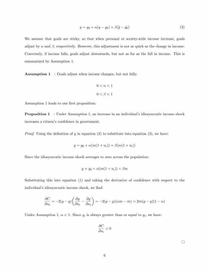
g = g0 + α(y − y0) + β(y − y0) (3)

We assume that goals are sticky, so that when personal or society-wide income increase, goals

adjust by α and β, respectively. However, this adjustment is not as quick as the change in income.

Conversely, if income falls, goals adjust downwards, but not as far as the fall in income. This is

summarized by Assumption 1.

Assumption 1 : Goals adjust when income changes, but not fully.

0 < α < 1

0 < β < 1

Assumption 1 leads to our first proposition:

Proposition 1 : Under Assumption 1, an increase in an individual’s idiosyncratic income shock

increases a citizen’s confidence in government.

Proof. Using the definition of y in equation (2) to substitute into equation (3), we have:

g = g0 + α(m(1 + ui)) + β(m(1 + ui))

Since the idiosyncratic income shock averages to zero across the population:

g = g0 + α(m(1 + ui)) + βm

Substituting this into equation (1) and taking the derivative of confidence with respect to the

individual’s idiosyncratic income shock, we find:

∂C

∂ui= −2(g − y)

(∂g

∂ui− ∂y

∂ui

)= −2(g − y)(αm−m) = 2m(g − y)(1 − α)

Under Assumption 1, α < 1. Since gi is always greater than or equal to yi, we have:

∂C

∂ui> 0

6

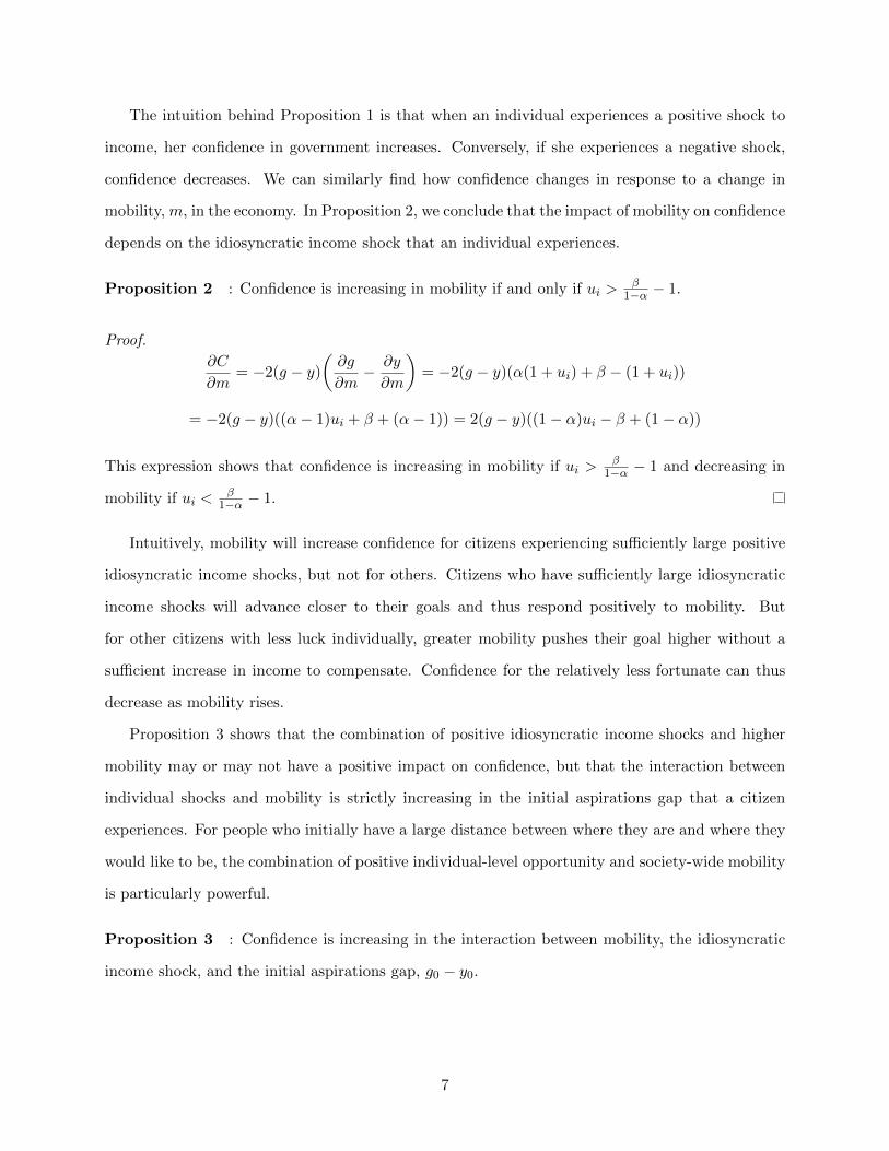
The intuition behind Proposition 1 is that when an individual experiences a positive shock to

income, her confidence in government increases. Conversely, if she experiences a negative shock,

confidence decreases. We can similarly find how confidence changes in response to a change in

mobility, m, in the economy. In Proposition 2, we conclude that the impact of mobility on confidence

depends on the idiosyncratic income shock that an individual experiences.

Proposition 2 : Confidence is increasing in mobility if and only if ui >β

1−α − 1.

Proof.

∂C

∂m= −2(g − y)

(∂g

∂m− ∂y

∂m

)= −2(g − y)(α(1 + ui) + β − (1 + ui))

= −2(g − y)((α− 1)ui + β + (α− 1)) = 2(g − y)((1 − α)ui − β + (1 − α))

This expression shows that confidence is increasing in mobility if ui >β

1−α − 1 and decreasing in

mobility if ui <β

1−α − 1.

Intuitively, mobility will increase confidence for citizens experiencing sufficiently large positive

idiosyncratic income shocks, but not for others. Citizens who have sufficiently large idiosyncratic

income shocks will advance closer to their goals and thus respond positively to mobility. But

for other citizens with less luck individually, greater mobility pushes their goal higher without a

sufficient increase in income to compensate. Confidence for the relatively less fortunate can thus

decrease as mobility rises.

Proposition 3 shows that the combination of positive idiosyncratic income shocks and higher

mobility may or may not have a positive impact on confidence, but that the interaction between

individual shocks and mobility is strictly increasing in the initial aspirations gap that a citizen

experiences. For people who initially have a large distance between where they are and where they

would like to be, the combination of positive individual-level opportunity and society-wide mobility

is particularly powerful.

Proposition 3 : Confidence is increasing in the interaction between mobility, the idiosyncratic

income shock, and the initial aspirations gap, g0 − y0.

7

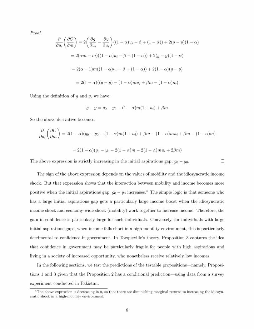
Proof.

∂

∂ui

(∂C

∂m

)= 2

(∂g

∂ui− ∂y

∂ui

)((1 − α)ui − β + (1 − α)) + 2(g − y)(1 − α)

= 2(αm−m)((1 − α)ui − β + (1 − α)) + 2(g − y)(1 − α)

= 2(α− 1)m((1 − α)ui − β + (1 − α)) + 2(1 − α)(g − y)

= 2(1 − α)((g − y) − (1 − α)mui + βm− (1 − α)m)

Using the definition of g and y, we have:

g − y = g0 − y0 − (1 − α)m(1 + ui) + βm

So the above derivative becomes:

∂

∂ui

(∂C

∂m

)= 2(1 − α)(g0 − y0 − (1 − α)m(1 + ui) + βm− (1 − α)mui + βm− (1 − α)m)

= 2(1 − α)(g0 − y0 − 2(1 − α)m− 2(1 − α)mui + 2βm)

The above expression is strictly increasing in the initial aspirations gap, g0 − y0.

The sign of the above expression depends on the values of mobility and the idiosyncratic income

shock. But that expression shows that the interaction between mobility and income becomes more

positive when the initial aspirations gap, g0 − y0 increases.4 The simple logic is that someone who

has a large initial aspirations gap gets a particularly large income boost when the idiosyncratic

income shock and economy-wide shock (mobility) work together to increase income. Therefore, the

gain in confidence is particularly large for such individuals. Conversely, for individuals with large

initial aspirations gaps, when income falls short in a high mobility environment, this is particularly

detrimental to confidence in government. In Tocqueville’s theory, Proposition 3 captures the idea

that confidence in government may be particularly fragile for people with high aspirations and

living in a society of increased opportunity, who nonetheless receive relatively low incomes.

In the following sections, we test the predictions of the testable propositions—namely, Proposi-

tions 1 and 3 given that the Proposition 2 has a conditional prediction—using data from a survey

experiment conducted in Pakistan.

4The above expression is decreasing in u, so that there are diminishing marginal returns to increasing the idiosyn-cratic shock in a high-mobility environment.

8

Data

Our results come from an original survey conducted in rural Pakistan in March – April 2012

(Round 1) and April – May 2013 (Round 2). In Round 1, we collected all demographic variables

and carried out a large module on individuals’ aspirations, attitudes, and cognitive processes.

In Round 2, the data collection included the experimental treatment, as well as a governance

module.5 In other words, aside for our outcome measures, all measures were collected prior to

the experiment. The one year time lag between the measurement of our moderating variables,

demographic characteristics, and our outcome variables is advantageous as we can rule out the

possibility that our experimental treatments impacted the moderating and demographic variables.

The survey covered 2,090 households in 76 villages in Punjab, Sindh, and Khyber-Pakhtunkhwa

(KPK) provinces.6 The head of each household and his/her spouse completed household surveys.7

We included a module on aspirations in Round 1 of the survey, following the module carried out by

Bernard, Taffesse, and Dercon (2008). The governance module carried out in Round 2 begins with

an experiment, described in the next section, before asking respondents a series of questions about

their political attitudes. A detailed description of each measure is provided in the measurement

section below. To ensure that variation in results is not due to using different samples, we restrict

our estimation sample to the 1,540 individuals with complete responses on all questions.

Research Design

We employ a 2 (poverty prime, no poverty prime) × 2 (mobility prime, no mobility prime)

research design to exogenously manipulate individual perceptions of their own poverty level and

possibilities for upward mobility in Pakistan.8 We then observe how these primes individually and

5In Round 2, we did not re-collect information on demographics like gender, age, and education level. We alsodid not re-administer the Round 1 aspirations module.

6The RHPS provides village-, household-, and individual-level data on a range of economic, political, and socialtopics. The RHPS sample was selected using a multi-stage, stratified sampling technique. 19 districts were selected:12 from Punjab, five from Sindh, and two from KPK. The sampling frame excluded Balochistan, the FederallyAdministered Tribal Areas, and 13 of KPK’s 24 districts due to safety concerns. Districts in each province wereselected using a probability proportionate to size approach. In each district, four mauzas (villages) were randomlyselected, and then 28 households were randomly chosen from each village. Urban villages and those with populationsgreater than 25,000 were excluded from the sampling frame.

7In cases where the head or spouse was not available, a second visit was made to the household. If the individualwas still not available, another knowledgeable household member of the same gender was selected instead.

8As shown in the balance tests displayed in Table A.1 in Online Appendix A, random assignment was successful.

9

jointly affect confidence in government, and how their impacts vary according to an individual’s

initial aspirations gap. In this section, we first explain the experimental treatments. We then outline

our outcome measures and how we measure the aspirations gap given that our theory predicts that

the effects of poverty and mobility are impacted by one’s initial aspirations gap. Finally, we describe

the empirical strategy to test our model’s propositions.

The Poverty Prime Treatment

Study participants were either induced to feel relatively poor, which we refer to as receiving

a poverty prime, or they were assigned to a control condition designed to frame their income

neutrally. The half assigned to the relatively poor condition were primed to feel that their income

was in the bottom part of the income distribution. The half assigned to the control condition were

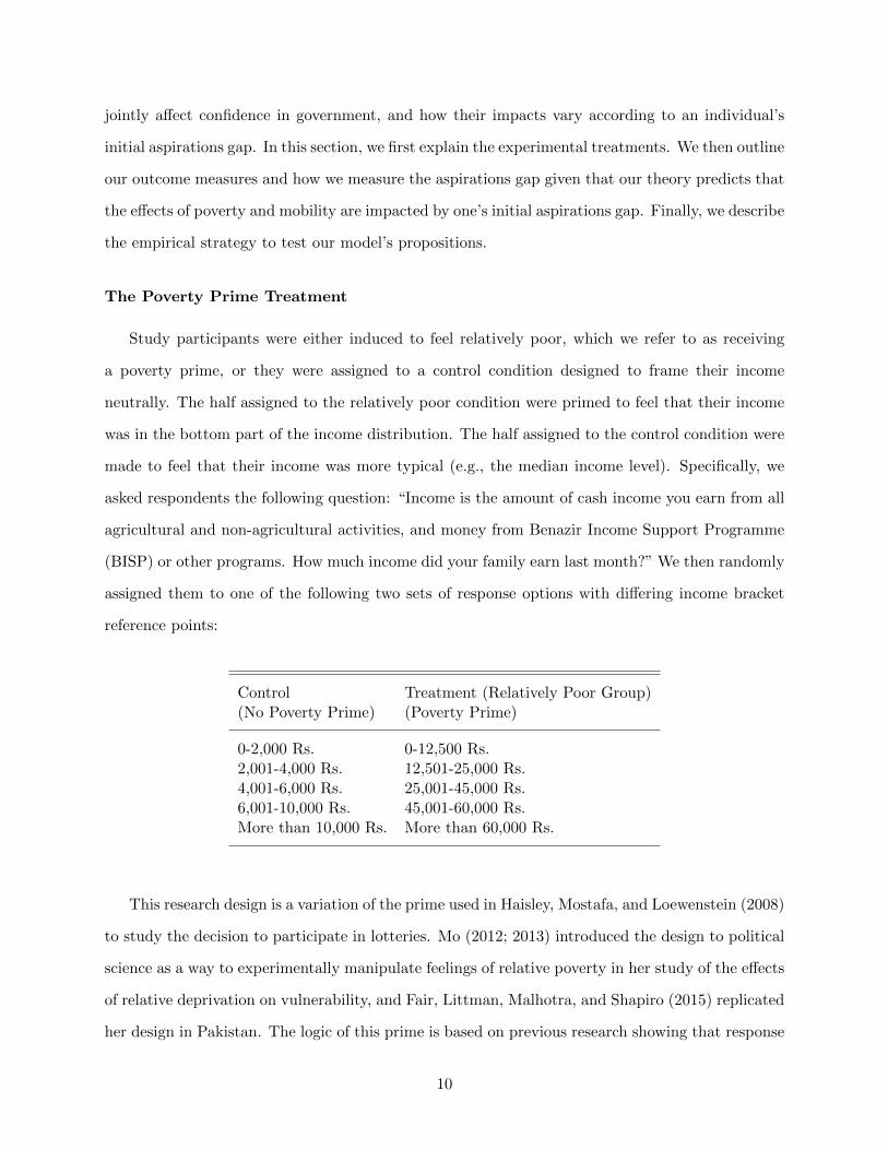
made to feel that their income was more typical (e.g., the median income level). Specifically, we

asked respondents the following question: “Income is the amount of cash income you earn from all

agricultural and non-agricultural activities, and money from Benazir Income Support Programme

(BISP) or other programs. How much income did your family earn last month?” We then randomly

assigned them to one of the following two sets of response options with differing income bracket

reference points:

Control Treatment (Relatively Poor Group)(No Poverty Prime) (Poverty Prime)

0-2,000 Rs. 0-12,500 Rs.2,001-4,000 Rs. 12,501-25,000 Rs.4,001-6,000 Rs. 25,001-45,000 Rs.6,001-10,000 Rs. 45,001-60,000 Rs.More than 10,000 Rs. More than 60,000 Rs.

This research design is a variation of the prime used in Haisley, Mostafa, and Loewenstein (2008)

to study the decision to participate in lotteries. Mo (2012; 2013) introduced the design to political

science as a way to experimentally manipulate feelings of relative poverty in her study of the effects

of relative deprivation on vulnerability, and Fair, Littman, Malhotra, and Shapiro (2015) replicated

her design in Pakistan. The logic of this prime is based on previous research showing that response

10

options to ordinal or interval questions can send cues—in those experiments, unintended cues—to

respondents about what responses are normal (e.g. Courneya, Jones, Rhodes, and Blanchard 2003;

Menon, Raghubir, and Schwarz 1997; Rockwood, Sangster, and Dillman 1997; Shwarz, Hipper,

Deutsch, and Strack 1985). Research has shown that respondents frequently assume that the

ranges offered by a question were purposely selected so that the middle response is the modal or

most customary response. The midpoint response changes the reference point on which respondents

focus, and their sense of economic well-being is then assessed in relation to this reference point.

Research in decision making, economics, and psychology has repeatedly found that people do not

simply evaluate the absolute value of income, performance, achievements, status, etc. (Crosby

1976; Festinger 1954; Suls and Wheeler 2000; Walker and Smith 2001). Rather, these evaluations

are heavily influenced by comparisons with others, and reference points can significantly impact

how people feel and make decisions (Heath, Larrick, and Wu 1999; Kahneman and Tversky 1979).

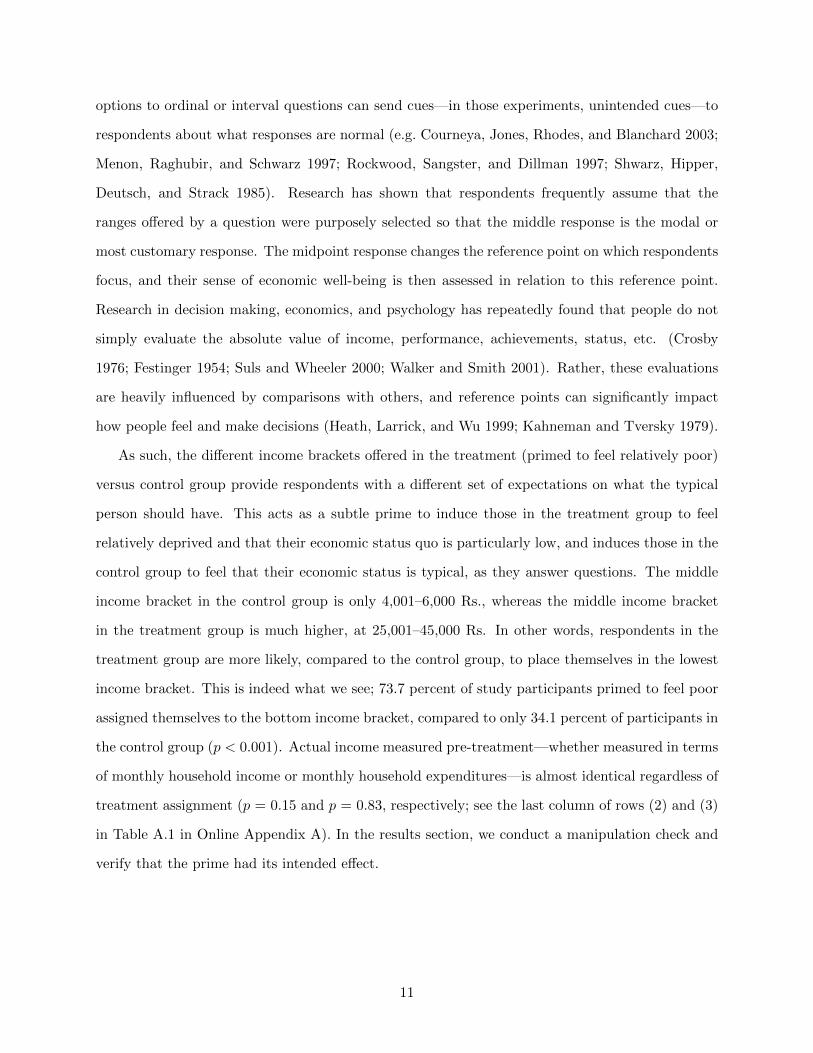
As such, the different income brackets offered in the treatment (primed to feel relatively poor)

versus control group provide respondents with a different set of expectations on what the typical

person should have. This acts as a subtle prime to induce those in the treatment group to feel

relatively deprived and that their economic status quo is particularly low, and induces those in the

control group to feel that their economic status is typical, as they answer questions. The middle

income bracket in the control group is only 4,001–6,000 Rs., whereas the middle income bracket

in the treatment group is much higher, at 25,001–45,000 Rs. In other words, respondents in the

treatment group are more likely, compared to the control group, to place themselves in the lowest

income bracket. This is indeed what we see; 73.7 percent of study participants primed to feel poor

assigned themselves to the bottom income bracket, compared to only 34.1 percent of participants in

the control group (p < 0.001). Actual income measured pre-treatment—whether measured in terms

of monthly household income or monthly household expenditures—is almost identical regardless of

treatment assignment (p = 0.15 and p = 0.83, respectively; see the last column of rows (2) and (3)

in Table A.1 in Online Appendix A). In the results section, we conduct a manipulation check and

verify that the prime had its intended effect.

11

The Mobility Prime Treatment

In a multitude of laboratory and survey contexts, a range of subtle interventions have been

shown to activate hypothesized attitude changes and behaviors. We draw on extant research on

primes (e.g., Berger, Meredith, and Wheeler 2008; DeMarree, Wheeler, and Petty 2005; Lodge and

Taber 2005) to assess the impact of perceived mobility on confidence in government. To exogenously

change how study participants felt about whether Pakistan offers high levels of economic mobility,

respondents were randomly assigned to receive the following information about economic mobility in

Pakistan, drawn from Corak (2012): “A 2012 study of 22 countries conducted by the Organization

for Economic Cooperation and Development has found that Pakistan offers higher mobility – the

ability of an individual or family to improve their economic and social status – than the United

States, the United Kingdom, Italy, China, and 5 other countries.”9 In other words, half of our

respondents received this mobility priming information to increase their perception that it is possible

to increase their economic and social status in Pakistan, and the other half received no such

information before being asked questions about their political attitudes.

In the results section, we implement a manipulation check and show that this prime was suc-

cessful. The measure we use to conduct this test is described in the measurement section below.

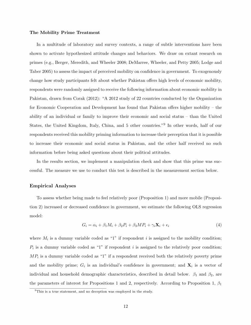
Empirical Analyses

To assess whether being made to feel relatively poor (Proposition 1) and more mobile (Proposi-

tion 2) increased or decreased confidence in government, we estimate the following OLS regression

model:

Gi = αi + β1Mi + β2Pi + β3MPi + γiXi + εi (4)

where Mi is a dummy variable coded as “1” if respondent i is assigned to the mobility condition;

Pi is a dummy variable coded as “1” if respondent i is assigned to the relatively poor condition;

MPi is a dummy variable coded as “1” if a respondent received both the relatively poverty prime

and the mobility prime; Gi is an individual’s confidence in government; and Xi is a vector of

individual and household demographic characteristics, described in detail below. β1 and β2, are

the parameters of interest for Propositions 1 and 2, respectively. According to Proposition 1, β1

9This is a true statement, and no deception was employed in the study.

12

should be a negative and statistically significant predictor. According to Proposition 2, the sign

and statistical significance of β2 is ambiguous, as the sign depends upon the extent to which an

individual’s goals adjust when personal income (α from Assumption 1 in the formal model) and the

income of others in the economy (β from Assumption 1 in the our formal model) change. Standard

errors are clustered at the household level since many of the factors influencing political attitudes

vary at the household level.

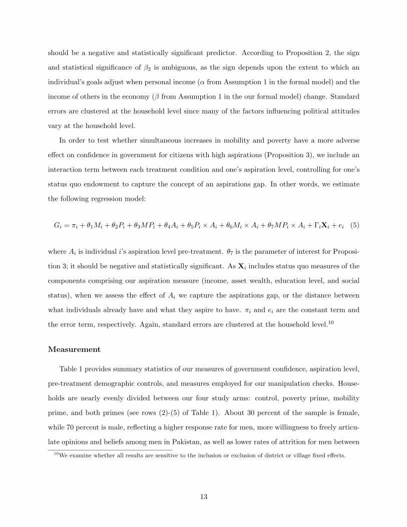
In order to test whether simultaneous increases in mobility and poverty have a more adverse

effect on confidence in government for citizens with high aspirations (Proposition 3), we include an

interaction term between each treatment condition and one’s aspiration level, controlling for one’s

status quo endowment to capture the concept of an aspirations gap. In other words, we estimate

the following regression model:

Gi = πi + θ1Mi + θ2Pi + θ3MPi + θ4Ai + θ5Pi ×Ai + θ6Mi ×Ai + θ7MPi ×Ai + ΓiXi + ei (5)

where Ai is individual i’s aspiration level pre-treatment. θ7 is the parameter of interest for Proposi-

tion 3; it should be negative and statistically significant. As Xi includes status quo measures of the

components comprising our aspiration measure (income, asset wealth, education level, and social

status), when we assess the effect of Ai we capture the aspirations gap, or the distance between

what individuals already have and what they aspire to have. πi and ei are the constant term and

the error term, respectively. Again, standard errors are clustered at the household level.10

Measurement

Table 1 provides summary statistics of our measures of government confidence, aspiration level,

pre-treatment demographic controls, and measures employed for our manipulation checks. House-

holds are nearly evenly divided between our four study arms: control, poverty prime, mobility

prime, and both primes (see rows (2)-(5) of Table 1). About 30 percent of the sample is female,

while 70 percent is male, reflecting a higher response rate for men, more willingness to freely articu-

late opinions and beliefs among men in Pakistan, as well as lower rates of attrition for men between

10We examine whether all results are sensitive to the inclusion or exclusion of district or village fixed effects.

13

rounds.11 92 percent of respondents are married, 44 percent have received no formal education,

and the average household has 6.2 members.

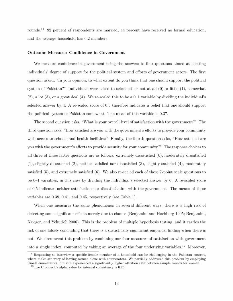
Outcome Measure: Confidence in Government

We measure confidence in government using the answers to four questions aimed at eliciting

individuals’ degree of support for the political system and efforts of government actors. The first

question asked, “In your opinion, to what extent do you think that one should support the political

system of Pakistan?” Individuals were asked to select either not at all (0), a little (1), somewhat

(2), a lot (3), or a great deal (4). We re-scaled this to be a 0–1 variable by dividing the individual’s

selected answer by 4. A re-scaled score of 0.5 therefore indicates a belief that one should support

the political system of Pakistan somewhat. The mean of this variable is 0.37.

The second question asks, “What is your overall level of satisfaction with the government?” The

third question asks, “How satisfied are you with the government’s efforts to provide your community

with access to schools and health facilities?” Finally, the fourth question asks, “How satisfied are

you with the government’s efforts to provide security for your community?” The response choices to

all three of these latter questions are as follows: extremely dissatisfied (0), moderately dissatisfied

(1), slightly dissatisfied (2), neither satisfied nor dissatisfied (3), slightly satisfied (4), moderately

satisfied (5), and extremely satisfied (6). We also re-scaled each of these 7-point scale questions to

be 0–1 variables, in this case by dividing the individual’s selected answer by 6. A re-scaled score

of 0.5 indicates neither satisfaction nor dissatisfaction with the government. The means of these

variables are 0.38, 0.41, and 0.45, respectively (see Table 1).

When one measures the same phenomenon in several different ways, there is a high risk of

detecting some significant effects merely due to chance (Benjamini and Hochberg 1995; Benjamini,

Krieger, and Yekutieli 2006). This is the problem of multiple hypothesis testing, and it carries the

risk of one falsely concluding that there is a statistically significant empirical finding when there is

not. We circumvent this problem by combining our four measures of satisfaction with government

into a single index, computed by taking an average of the four underlying variables.12 Moreover,

11Requesting to interview a specific female member of a household can be challenging in the Pakistan context,where males are wary of leaving women alone with enumerators. We partially addressed this problem by employingfemale enumerators, but still experienced a significantly higher attrition rate between sample rounds for women.

12The Cronbach’s alpha value for internal consistency is 0.75.

14

the advantage of an averaged measure is that it nets out measurement error associated with any one

of the index components (Ansolabehere, Rodden, and Snyder 2008). Our government confidence

index has a mean of 0.40 and a standard deviation of 0.23. If we detect significant changes in this

index, we can be relatively confident that they reflect true changes in confidence in government,

as opposed to errors in the measurement of a single dimension yielding a spurious correlation. We

consider each of the four measures separately as a robustness check.

Aspiration Level

We measure an individual’s pre-treatment aspiration level using an index similar to that used

by Bernard and Seyoum Taffesse (2014). The index is constructed using respondents’ answers

to questions about their aspirations along four dimensions: income, asset wealth, education, and

social status. Specifically, respondents were asked to report the level of personal income, the value

of assets, the level of education (re-coded as desired years of education), and the level of social

status (on a 10-step ladder of possibilities) they would like to achieve. While there is a potentially

infinite number of dimensions on which an individual could aspire, we argue that these four capture

a large and important share of aspirations. Question wording can be found in Online Appendix B.

We combined these four aspiration levels into an index using the following methodology. First,

we normalized each respondent’s aspiration level on each dimension by subtracting the average

level for individuals in the same district (there are 19 districts in our sample), and then dividing

this difference by the standard deviation for individuals in the same district.13 We examine the

individual’s aspirations relative to the district, as an individual’s aspiration levels are affected

by a process of social comparison with others in the individual’s social environment or reference

group (e.g., Festinger 1954; Merton and Rossi 1950; Suls and Wheeler 2000). We then asked each

individual to allocate 20 beans across the four dimensions according to their relative importance,

and weighted each dimension by the share of beans placed on it. This yields the following index:

Aspiration Level =

4∑n=1

(ain − µinσdn

)win (6)

13The resulting, normalized outcome represents the number of standard deviations from the district average thatan individual’s aspired level is located. Respondents with an aspiration level for a particular outcome above theirdistrict’s average have a positive value on the normalized outcome, while those with a level below the average havea negative value.

15

where ain is the aspired outcome of individual i on dimension n (income, asset wealth, education,

or social status); and µdn is the average aspired outcome in district d for outcome n. The standard

deviation of aspired outcomes in district d for outcome n is σdn. Finally, win is the weight individual i

places on dimension n, and these four weights sum to 1.14 Poverty and economic opportunities vary

widely across districts. To the extent that the district average aspiration level represents what is

typically possible to achieve in a district, our measure of aspirations captures the distance between

what is generally possible and what an individual aspires to achieve.

Table 1 includes summary statistics for our aspiration level index. The average individual has

an aspiration level of 0.10, with a standard deviation of 0.67. The aspiration level takes both

negative and positive values given it is a normalized measure, and its mean is close to 0.15

Demographic Characteristics

We consider several demographic controls in all analysis that consider aspiration levels.16 We

aimed to control for those features of an individual that should have a direct impact on their

aspiration level, as measured by our aspiration index. These include their current logged household

income, logged household asset wealth, social status (on a 1 through 10 scale), and education

level (no formal education, primary education, middle education, high/intermediate education,

and post-secondary education).17 Inclusion of these controls lends our aspiration index measure

the interpretation of reflecting an aspirations gap, since it measures aspirations after accounting

for status quo endowments.

Given our reliance on randomization of treatment in the context of an experiment, we can

identify the causal impacts of our poverty and mobility primes without the need for other controls.

Nonetheless, including several controls can increase the precision of our estimates, in case there

are small imbalances across treatment arms. Indeed, as shown in the balance tests in Table A.1

in Online Appendix A, we have select cases of imbalance. For example, those that received the

mobility prime have slightly higher incomes than do those that did not receive any prime, and

14Note that the index is a weighted average of four normally distributed variables with mean 0 and standarddeviation 1. However, it is not itself distributed normally with mean 0 and standard deviation 1.

15While the aspiration level is a weighted average of four N(0,1) variables, it is not itself distributed N(0,1).16All of these measures were collected at the time of our Round 1 (2012) survey to ensure these measures are 1)

all pre-treatment measures; and 2) collected when questions on aspiration levels were asked.17Question wording for these questions can be found in Online Appendix B.

16

those that received both primes also have slightly higher incomes than do those that received no

prime. Also, those that received both primes have fathers with slightly more education than do

those that did not receive any prime or those that received only the mobility prime. Nevertheless,

out of 30 joint tests of imbalance, there are only two cases of imbalance between treatment groups

(i.e., where p < 0.10), which suggests that random assignment was highly successful.

We control for a measure of the individual’s level of trust in others, and their degree of envy of

others, given that they may be correlated with attitudes toward government and our poverty and

mobility treatments.18 We also control for key demographic characteristics that might influence

political opinions. These include their father’s education level (in years), mother’s education level

(in years), gender,19 age group (18–25, 25–35, 35–45, 45–55, and over 55), ethnicity,20 and household

size. Finally, we estimate specifications with district fixed effects and village fixed effects.

Results

Our main regression results that test the “Tocqueville Effect” appear in Table 2, where the

outcome is our government confidence index. Column (1) shows our baseline results.21 Those

randomly assigned to receive only the poverty prime, which causes individuals to feel relatively

poor, report significantly lower satisfaction with government than do those who received no primes;

this is consistent with Proposition 1 (p = 0.04). Receiving only the poverty prime leads to a 3.4

percentage point reduction in government satisfaction (see column (1) of Table 2); this is a sizable,

8.5 percent decrease relative to the mean value of the government confidence index. This effect size

is especially large in light of this being a survey experiment; rather than actually making individuals

relatively poorer, our treatment subtly primes them to feel this way. One might expect even larger

impacts on confidence in government if we actually and permanently changed individuals’ relative

welfare. This suggests that if anything, our estimates are lower bounds on the magnitude of the

18Trust and envy are both measured as indices computed based on a grouping of questions that were normalized(by subtracting the sample mean and then dividing by the sample standard deviation) and then averaged over thegroup. In the case of trust, there were 12 questions. In the case of envy, there were 3 questions. A complete list ofquestions is available in Kosec and Khan (2016).

19Female is coded as 1.20We include fixed effects for each ethnic group.21Regression results equivalent to column (1) of Table 2 for each of the confidence measures that make up the index

are shown in columns (1), (3), (5), (7), and (9) in Table A.2 in Online Appendix A. We also visualize these resultsin Figure A.1 in Online Appendix A.

17

impacts on confidence in government resulting from feeling relatively poor. The magnitude and

significance of this result is not sensitive to the inclusion of district or village fixed effects or

demographic control variables (columns (2)–(4)), which provides reassurance that the randomized

experiment was implemented correctly.22

Receiving only the mobility prime leads to no substantive change in the government confidence

index (β = -0.014; p = 0.38; see column (1) of Table 2), and this effect is further statistically

insignificant at conventional levels. This result is consistent with Proposition 2 of our formal

model, which shows that mobility has a positive effect on government confidence for some and

a negative effect for others. Finally, we see no significant impact on government confidence for

those who received both primes (β = 0.007; p = 0.70). The negative impact on confidence in

government of being primed to feel relatively poor is, on average, neutralized when individuals are

simultaneously primed to feel mobile. Again, the findings in column (1) are robust to the inclusion

of district or village fixed effects and demographic controls.

When we interact each of our three treatment arm dummies (receipt of the mobility prime,

poverty prime, and both primes) with the individual’s aspiration level, we see evidence consistent

with Proposition 3, which captures the main thesis of Tocqueville (1856). Specifically, this thesis

predicts that confidence in government among high-aspiring citizens declines when their perceived

relative position decreases and perceived mobility increases, since these are the citizens that expe-

rience the greatest aspirations gap when they are made to feel both relatively poor and mobile.

As shown in column (1) of Table 3 and visualized in Figure 1(d),23 this is precisely what we find.

Among those with relatively high aspiration levels (and hence large aspirations gaps), receiving

both primes has a large and significant negative impact on confidence in government—specifically,

a 6.6 percentage point reduction in satisfaction for every one-unit increase in aspirations (p =

0.007; see column (1) of Table 3). This is a large, 16.4 percent decrease in government confidence

relative to the mean of the index. This negative effect is statistically significant for each of the four

individual measures that make up the government confidence index as well, as shown in Figure

22The effect size ranges from 3.2 to 3.6 percentage points depending on the specification, and effects are statisticallysignificant regardless of the specification (p-values range from 0.02 to 0.04).

23We consider the association between aspiration level and the government confidence index for each of the fourconditions separately—(1) receipt of no prime (Figure 1(a)); (2) receipt of only the mobility prime (Figure 1(b)); (3)receipt of only the poverty prime (Figure 1(c)); and (4) receipt of both primes (Figure 1(d)).

18

2.24 Moreover, these findings are robust to the inclusion of district or village fixed effects and

demographic controls. We take this as strong evidence supporting Proposition 3 and Tocqueville’s

verbal hypothesis.

As in our results without interactions with the aspirations gap, receiving the mobility prime

alone once again has both an economically and statistically insignificant effect on confidence in

government—and this effect also does not vary with the aspirations gap (see row (4) of Table 3 and

Figure 1(b)). Additionally, receiving the poverty prime alone is once again associated with lower

satisfaction with government (see row (2) of Table 3), and this effect does not vary according to

the individual’s aspirations gap (see Figure 1(c)).

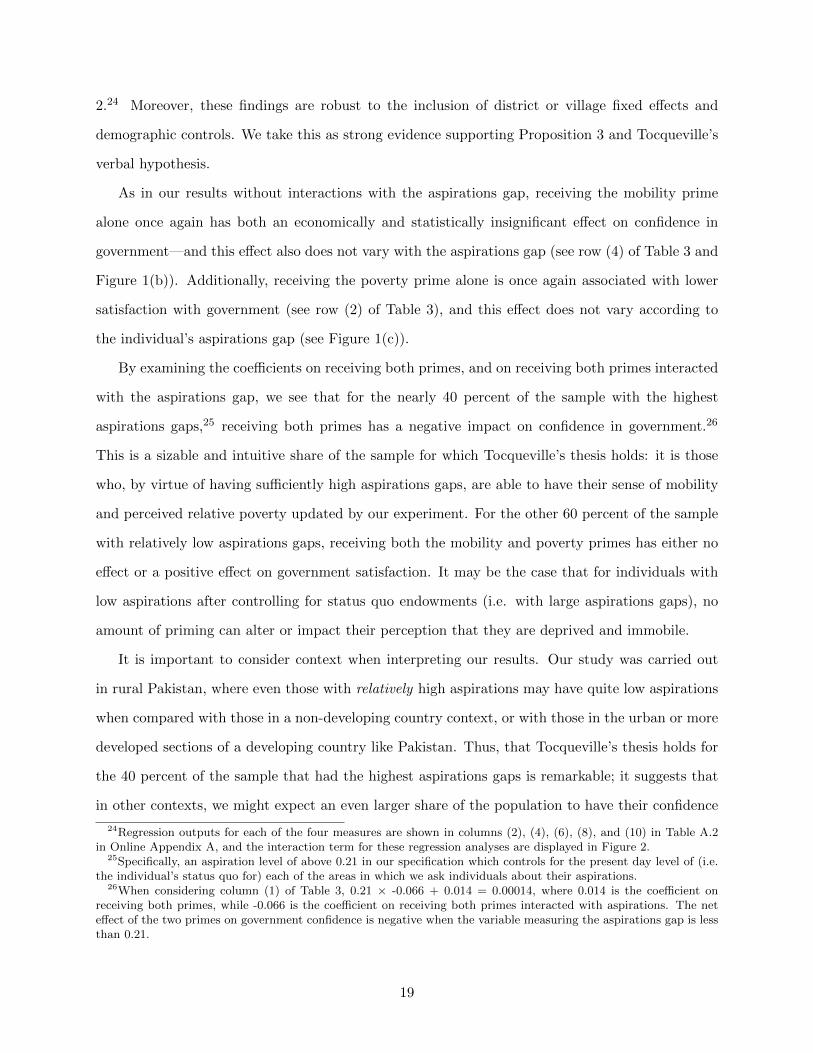
By examining the coefficients on receiving both primes, and on receiving both primes interacted

with the aspirations gap, we see that for the nearly 40 percent of the sample with the highest

aspirations gaps,25 receiving both primes has a negative impact on confidence in government.26

This is a sizable and intuitive share of the sample for which Tocqueville’s thesis holds: it is those

who, by virtue of having sufficiently high aspirations gaps, are able to have their sense of mobility

and perceived relative poverty updated by our experiment. For the other 60 percent of the sample

with relatively low aspirations gaps, receiving both the mobility and poverty primes has either no

effect or a positive effect on government satisfaction. It may be the case that for individuals with

low aspirations after controlling for status quo endowments (i.e. with large aspirations gaps), no

amount of priming can alter or impact their perception that they are deprived and immobile.

It is important to consider context when interpreting our results. Our study was carried out

in rural Pakistan, where even those with relatively high aspirations may have quite low aspirations

when compared with those in a non-developing country context, or with those in the urban or more

developed sections of a developing country like Pakistan. Thus, that Tocqueville’s thesis holds for

the 40 percent of the sample that had the highest aspirations gaps is remarkable; it suggests that

in other contexts, we might expect an even larger share of the population to have their confidence

24Regression outputs for each of the four measures are shown in columns (2), (4), (6), (8), and (10) in Table A.2in Online Appendix A, and the interaction term for these regression analyses are displayed in Figure 2.

25Specifically, an aspiration level of above 0.21 in our specification which controls for the present day level of (i.e.the individual’s status quo for) each of the areas in which we ask individuals about their aspirations.

26When considering column (1) of Table 3, 0.21 × -0.066 + 0.014 = 0.00014, where 0.014 is the coefficient onreceiving both primes, while -0.066 is the coefficient on receiving both primes interacted with aspirations. The neteffect of the two primes on government confidence is negative when the variable measuring the aspirations gap is lessthan 0.21.

19

in government reduced by simultaneously being primed to feel relatively poor and mobile.

Analysis of Prime Effectiveness and Manipulation Checks

Our analysis of how priming individuals to feel relatively poor and/or mobile impacts their

attitudes toward the government assumes that our experiment had its intended effect. That is,

priming individuals to feel relatively poor made them feel relatively poorer than they otherwise

would, and priming individuals to feel mobile made them feel more mobile and able to improve

on their current position than they otherwise would. Evidence from Mo (2012; 2013) in Nepal,

which was then replicated in Pakistan by Fair et al. (2015)—as well as the diagnostic statistics

on our poverty prime that we presented in the previous research design section on the poverty

prime treatment—suggest that our experimental method of priming individuals to feel poor had

the intended effect.

We are able to gain further verification that our treatment had its intended effect by examining

whether the poverty prime affected only those who did not feel poor to begin with. People that

already felt relatively poor should be somewhat immune to the prime. For this exercise, we can

leverage the following question collected prior to the experiment: “[Show the picture of a ladder]

Please look at this ladder, which has 10 steps. Suppose we say that the top of this ladder represents

the best possible life for you and the bottom step represents the worst possible life for you. Where

on the ladder do you feel you personally stand at present?” The median and mean response is 5,

the mid-point of the scale. We thus divided our sample into two groups: those who chose a number

of less than 5 and those who chose 5 or better. These two groups represent (A) those who already

feel low on a ladder of subjective well-being, and as such, should not feel the effects of a prime

designed to trigger feelings of relative poverty, and (B) those who feel well-off, and as such, have

room for their subjective well-being to fall in response to the prime.

We repeat the analyses of our main results in Table 2 and Table 3, which are described in

the results section above, for the two groups of interest: Columns (1)–(6) of Table A.3 in Online

Appendix A consider group (A), while columns (7)–(12) consider group (B).27 As expected, we see

27Columns (1) and (7), (2) and (8), and (3) and (9) in Table A.3 in Online Appendix A reproduce columns (1),(2), and (4) in Table 2, respectively. Columns (4) and (10), (5) and (11), and (6) and (12) of Table A.3 in OnlineAppendix A reproduce columns (1), (2), and (4) in Table 3, respectively.

20

that the negative effect of the poverty prime (test of Proposition 1), as well as the interaction be-

tween receipt of both the poverty and mobility prime and one’s aspirations gap (test of Proposition

3) are only seen for group (B)—the group with initially high levels of subjective well-bring. When

we consider the impact of receiving the poverty prime (test of Proposition 1), effect sizes for group

(B) range from -4.1 to -4.8 percentage points and are statistically significant. In contrast, effect

sizes for the group which had low subjective well-being before the prime (group (A)) range from

-0.6 to -1.4 percentage points and are statistically insignificant. The difference between the impact

on group (A) and the impact on group (B) is always highly statistically significant (p < 0.01). In

short, receiving the poverty prime lowers one’s confidence in government, but this is only the case

for those who we would actually expect to have their beliefs updated by the prime: those with

initially high subjective well-bring. When we next consider the interaction between the aspirations

gap and the dummy for receiving both the mobility and poverty primes (test of Proposition 3),

we find that it is also only statistically significant for group (B). The magnitude of the interaction

term for group (A) ranges from -0.001 to 0.004 and is in all cases statistically insignificant, while

for group (B) it ranges from -0.094 to -0.062 and is always statistically significant. Again, the

difference between these two sets of magnitudes is always highly statistically significant (p < 0.01).

Proposition 3 and Tocqueville’s verbal hypothesis are supported by the data, and these effects are

intuitively driven by those for whom we would expect the primes to have the greatest impact.

We do not know of any existing studies priming individuals to feel mobile. Fortunately, however,

we can statistically check that the mobility prime had the intended effect. We are able to do so

given that we asked all respondents the following question related to their perceived level of mobility

after receiving the mobility and/or poverty prime: “In your opinion, to what extent do people in

Pakistan get rewarded for their intelligence and skills?” Again, this variable is measured on a scale

from 0 to 1, where 0 indicates not at all, and 0.25, 0.5, 0.75, and 1 respectively indicate a little,

somewhat, a lot, and a great deal. The mean of this measure is 0.40, reflecting that individuals

tend to believe that mobility is not particularly high in Pakistan. An analysis of this questions

allows us to examine whether or not the mobility prime actually caused individuals to report that

they feel more mobile.

Table A.4 in Online Appendix A examines the effect of being primed to feel mobile (by having

been read our mobility script as part of the experiment) on an outcome variable indicating the

21

extent to which an individual feels that people in Pakistan are rewarded for their intelligence and

skills. As we see in column (1), receiving our mobility prime leads to a 3.6 percentage point increase

(p = 0.01) in this outcome variable. As this variable’s mean is 0.40, a 0.036 point increase represents

a 9 percent increase relative to the mean value. The size of this effect is largely unchanged when we

add district fixed effects (column (2)), a battery of pre-treatment control measures (column (5)),

and village fixed effects (column (6)). We take this as evidence that our mobility prime had its

intended effect. Moreover, we find no differential impacts of our primes according to an individual’s

aspiration level (and hence gap), as shown in columns (3) – (6) in Table A.4 in Online Appendix

A.28 Similarly, we find no evidence that the effect of the poverty prime on feelings of mobility varies

with one’s aspirations gap.29

Conclusion

Using an original experimental dataset collected in Pakistan during 2012–2013, we present

strong evidence in favor of a theory articulated by Tocqueville (1856). That theory suggests that

discontent with government can increase even when economic development creates opportunities for

economic and social mobility. For many citizens, expectations increase and personal circumstances

fail to keep up, creating political discontent. We formalize these insights by presenting a theoretical

model of the impacts of perceived poverty and economic mobility on confidence in government. Our

experimental evidence supports that model, and thus Tocqueville’s theory.

The experiment has the key advantage that it generates perceptions of higher relative poverty

and higher mobility which are exogenous to our attitudinal outcomes related to confidence in

government. However, it has the disadvantage that we subtly create only the (likely temporary)

perception that one is relatively poor. Perceptions of relative poverty may have a different effect

than does actually falling into deeper levels of poverty. Further research is needed on how confidence

28Columns (3) and (4) in particular replicate columns (1) and (2) but add a control for an individual’s aspirationlevel adjusting for present day socio-economic status levels to capture aspirations gaps, as well as its interaction witheach of the two primes.

29In other words, we do not find significant interaction terms between either of the two primes and our measureof aspiration levels adjusted for present day socio-economic status. The interaction between the mobility primeand the aspiration level is never statistically significant. While the interaction between the poverty prime and theaspiration level is weakly significant in column (3), this significance disappears when we include district fixed effects,pre-treatment demographic control measures, or village fixed effects. As such, any significance of the interaction termbetween the poverty prime and aspiration levels is not robust.

22

in, and support for, government varies with the combination of increases in one’s actual relative

poverty level and increases in one’s perceived mobility. Such research could, for example, consider

a natural experiment such as a natural disaster that impacts relative poverty levels for some subset

of a population.

Overall, our findings constitute an important theoretical and empirical contribution to the

literature on drivers of support for government. They help make sense of the somewhat paradoxical

claim articulated by Tocqueville (1856): that economic development and mobility do not always lead

to increased confidence in government, and may potentially erode it, triggering greater opposition

rather than support for their political leaders and system. They also help us understand which

citizens are most likely to oppose government when made to feel both relatively poor and mobile;

specifically, it is those with the highest aspiration levels to begin with, whose aspirations gaps

accordingly increase the most when made to feel both relatively poor and mobile. From an academic

perspective, this helps us better understand not only when acts of opposition to the government are

most likely to emerge, but also which groups of citizens are most likely to join in such opposition

and why. From a policy perspective, such information is useful for preventing state failure and

designing responsive public policies that include citizens in the development process.

23

References

Acemoglu, Daron, Georgy Egorov, and Konstantin Sonin. 2015. “Re-evaluating de Tocqueville:

Social Mobility and Stability of Democracy.” Working Paper, Massachusetts Institute of Tech-

nology.

Ansolabehere, Stephen, Jonathan Rodden, and James M. Jr. Snyder. 2008. “The Strength of

Issues: Using Multiple Measures to Gauge Preference Stability, Ideological Constraint, and Issue

Voting.” American Political Science Review 102(5): 215–232.

Benjamini, Yoav, Abba M Krieger, and Daniel Yekutieli. 2006. “Adaptive Linear Step-Up Proce-

dures that Control the False Discovery Rate.” Biometrika 93 (3): 491–507.

Benjamini, Yoav, and Yosef Hochberg. 1995. “Controlling the False Discovery Rate: a Practical

and Powerful Approach to Multiple Testing.” Journal of the Royal Statistical Society. Series B

(Methodological) 289–300.

Berger, Jonah, Marc Meredith, and S. Christian Wheeler. 2008. “Contextual Priming: Where

People Vote Affects How They Vote.” Proceedings of the National Academy of Sciences 105 (26):

8846–8849.

Bernard, Tanguy, and Alemayehu Seyoum Taffesse. 2014. “Aspirations: An Approach to Measure-

ment with Validation Using Ethiopian Data.” Journal of African Economies 23 (2): 189–224.

Blair, Dennis, Ronald Neumann, and Eric Olson. 2014. “Fixing Fragile States.” The National

Interest .

Blau, Peter M. Blau, and Otis D. Duncan. 1967. The American Occupational Structure. New York,

NY: John Wiley and Sons.

Central Intelligence Agency. 2015. “The World Factbook 2013-14.” Washington, DC: Central

Intelligence Agency.

Corak, Miles. 2012. “Economic Mobility Across the Generations in the United States: Comparisons,

Causes, and Consequences.” Written Testimony to the United States Senate, Committee on

Finance July 10th, 2012 Hearing on “Tax Reform: Drivers of Intergenerational Mobility and the

Tax Code.” http : //www.finance.senate.gov/imo/media/doc/Corak%20Testimony.pdf .

24

Courneya, Kerry S., Lee W. Jones, Ryan E. Rhodes, and Chris M. Blanchard. 2003. “Effect of

Response Scales on Self-Reported Exercise Frequency.” American Journal of Health Behavior 27

(6): 613–622.

Crosby, Faye. 1976. “A Model of Egoistic Relative Deprivation.” Psychological Review 83: 95–113.

DeMarree, Kenneth G., S. Christian Wheeler, and Richard E. Petty. 2005. “Priming a New Iden-

tity: Self-Monitoring Moderates the Effects of Nonself Primes on Self-Judgments and Behavior.”

Journal of Personality and Social Psychology 89 (5): 657–671.

Fair, Christine, Rebecca Littman, Neil Malhotra, and Jacob N. Shapiro. 2015. “Relative Poverty,

Perceived Violence, and Support for Militant Politics: Evidence from Pakistan.” Working Paper,

Stanford University.

Felbab-Brown, Vanda. 2010. “Rules and Regulations in Ungoverned Spaces: Illicit Economies,

Criminals, and Belligerents.” In Ungoverned Spaces: Alternatives to State Authority in an Era of

Softened Sovereignty, eds. Anne L. Clunan, and Harold A. Trinkunas. Stanford University Press

175–192.

Festinger, Leon. 1954. “A Theory of Social Comparison Processes.” Human Relations 7: 117–140.

Ghani, Ashraf, and Clare F. Lockhart. 2009. Fixing Failed States: A Framework for Rebuilding a

Fractured World. Cambridge: Oxford University Press.

Goldhammer, Arthur, and Jon Elster. 2011. Tocqueville: The Ancien Regime and the French

Revolution. Cambridge University Press.

Haisley, Emily, Romel Mostafa, and George Loewenstein. 2008. “Subjective Relative Income and

Lottery Ticket Purchases.” Journal of Behavioral Decision Making 21: 283–295.

Heath, Chip, Richard Larrick, and George Wu. 1999. “Goals as Reference Points.” Cognitive

Psychology 38: 79–109.

Hirschman, Albert O., and Michael Rothschild. 1973. “The Changing Tolerance for Income In-

equality in the Course of Economic Development.” Quarterly Journal of Economics 87: 544–566.

Kahneman, Daniel, and Amos Tversky. 1979. “Prospect Theory: An Analysis of Decision under

Risk.” Econometrica 47(March): 263–292.

25

Keidel, Albert. 2005. “The Economic Basis for Social Unrest in China.” Third European-American

Dialogue on China, Washington, DC, May 26-27.

Kosec, Katrina, and Huma Khan. 2016. “Understanding the Aspirations of the Rural Poor.” In

Agriculture and Rural Poverty Reduction in Pakistan, eds. David Spielman, Sohail Malik, Paul

Dorosh, and Nuzhat Ahmad. University of Pennsylvania Press.

Lamb, Robert D. 2008. “Ungoverned Areas and Threats from Safe Havens.” Office of the Deputy

Assistant Secretary of Defense for Policy Planning.

Lewis-Beck, Michael S. 1988. Economics and Elections: The Major Western Democracies. Ann

Arbor: University of Michigan Press.

Lewis-Beck, Michael Steven, and Richard Nadeau. 2011. “Economic Voting Theory: Testing New

Dimensions.” Electoral Studies 30 (2): 288 – 294.

Lipset, Seymour Martin. 1960. Political Man: The Social Bases of Politics. Baltimore, MD: The

Johns Hopkins University Press.

Lodge, Milton, and Charles S. Taber. 2005. “The Automaticity of Affect for Political Leaders,

Groups, and Issues: An Experimental Test of the Hot Cognition Hypothesis.” Political Psychology

26 (3): 8846–8849.

Menon, Geeta, Priya Raghubir, and Norbert Schwarz. 1997. “How Much Will I Spend? Factors

Affecting Consumers’ Estimates of Future Expense.” Journal of Consumer Psychology 6 (2):

141–164.

Mo, Cecilia. 2012. “Essays in Behavioral Political Economy: The Effects of Affect, Attitude, and As-

pirations.” Ph.D. Diss. Stanford University, Stanford, CA. http : //searchworks.stanford.edu/

view/9623096.

Mo, Cecilia. 2013. “The Effects of Perceived Relative Poverty on Risk: An Aspirations-Based Model

of Trafficking Vulnerability.” Working Paper, Vanderbilt University.

Moore, Barrington. 1966. Social Origins of Dictatorship and Democracy. Boston, Massachusetts:

Beacon Press.

Patrick, Stewart. 2010. “Are Ungoverned Spaces a Threat?” Expert Brief for the Council on

Foreign Relations, January 11.

26

Ray, Debraj. 2006. “Aspirations, Poverty and Economic Change.” In Understanding Poverty, eds.

Abhijit V. Banerjee, Roland Benabou, and Dilip Mookherjee. Oxford, UK: Oxford University

Press, 409–443.

Rockwood, Todd H., Roberta L. Sangster, and Don A. Dillman. 1997. “The Effect of Response

Categories on Questionnaire Answers.” Sociological Methods and Research 26 (1): 118–149.

Shwarz, Norbert, Hans J. Hipper, Brigitte Deutsch, and Fritz Strack. 1985. “Response Scales:

Effects of Category Range on Reported Behavior and Comparative Judgments.” Public Opinion

Quarterly 49: 388–395.

Suls, Jerry M., and Ladd Wheeler. 2000. Handbook of Social Comparison: Theory and Research.

New York, NY: Kluwer Academic/Plenum Publishers.

Tocqueville, Alexis de. 1835. Democracy in America. trans. Henry Reeve. South Australia: The

University of Adelaide.

Tocqueville, Alexis de. 1856. The Old Regime and the Revolution. trans. by John Bonner. New

York, NY: Harper Press.

Walker, Iain, and Heather J. Smith. 2001. Relative Deprivation: Specification, Development and

Integration. Cambridge: Cambridge University Press.

27

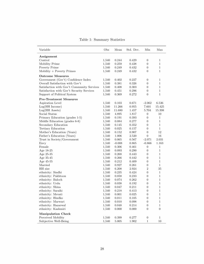
Table 1: Summary Statistics

Variable Obs Mean Std. Dev. Min Max

AssignmentControl 1,540 0.244 0.429 0 1Mobility Prime 1,540 0.259 0.438 0 1Poverty Prime 1,540 0.249 0.432 0 1Mobility + Poverty Primes 1,540 0.249 0.432 0 1

Outcome MeasuresGovernment (Gov’t) Confidence Index 1,540 0.402 0.227 0 1Overall Satisfaction with Gov’t 1,540 0.381 0.326 0 1Satisfaction with Gov’t Community Services 1,540 0.408 0.303 0 1Satisfaction with Gov’t Security Services 1,540 0.451 0.296 0 1Support of Political System 1,540 0.369 0.272 0 1

Pre-Treatment MeasuresAspiration Level 1,540 0.103 0.671 -2.062 6.536Log(HH Income) 1,540 11.266 0.955 7.601 15.425Log(HH Assets) 1,540 11.680 1.457 5.704 15.398Social Status 1,540 4.895 1.817 0 10Primary Education (grades 1-5) 1,540 0.191 0.393 0 1Middle Education (grades 6-8) 1,540 0.084 0.277 0 1Secondary Education 1,540 0.145 0.352 0 1Tertiary Education 1,540 0.025 0.157 0 1Mother’s Education (Years) 1,540 0.152 0.907 0 12Father’s Education (Years) 1,540 1.006 2.520 0 16Trust in Society/Government 1,540 0.065 0.567 -2.071 2.031Envy 1,540 -0.008 0.865 -0.866 1.163Female 1,540 0.306 0.461 0 1Age 18-25 1,540 0.093 0.290 0 1Age 25-35 1,540 0.268 0.443 0 1Age 35-45 1,540 0.266 0.442 0 1Age 45-55 1,540 0.212 0.409 0 1Married 1,540 0.927 0.261 0 1HH size 1,540 6.208 2.924 2 35ethnicity: Sindhi 1,540 0.235 0.424 0 1ethnicity: Pakhtoon 1,540 0.058 0.233 0 1ethnicity: Baloch 1,540 0.074 0.262 0 1ethnicity: Urdu 1,540 0.038 0.192 0 1ethnicity: Shina 1,540 0.047 0.211 0 1ethnicity: Saraiki 1,540 0.218 0.413 0 1ethnicity: Mevati 1,540 0.001 0.025 0 1ethnicity: Hindko 1,540 0.011 0.105 0 1ethnicity: Marwari 1,540 0.010 0.098 0 1ethnicity: Hazarwal 1,540 0.048 0.214 0 1ethnicity: Kashmiri 1,540 0.000 0.000 0 0

Manipulation CheckPerceived Mobility 1,540 0.399 0.277 0 1Subjective Well-Being 1,540 5.005 1.902 1 10

28

Table 2: Impact of Mobility and Relative Poverty on Government Confidence

(1) (2) (3) (4)

Mobility Prime -0.014 -0.013 -0.015 -0.012(0.016) (0.015) (0.015) (0.015)

Poverty Prime -0.034** -0.033** -0.036** -0.032**(0.016) (0.015) (0.015) (0.015)

Mobility + Poverty Primes 0.007 0.008 0.006 0.004(0.017) (0.015) (0.015) (0.015)

Aspiration Level 0.000 -0.002(0.010) (0.011)

Log(HH Income) -0.001 -0.003(0.008) (0.008)

Log(HH Assets) 0.002 0.003(0.005) (0.005)

Social Status -0.004 -0.003(0.004) (0.004)

Primary Education -0.024* -0.018(0.015) (0.015)

Middle School Education -0.027 -0.023(0.023) (0.022)

Secondary Education 0.037* 0.044**(0.020) (0.020)

Tertiary Education 0.029 0.031(0.045) (0.043)

Mother’s Education -0.012** -0.010*(0.006) (0.006)

Father’s Education 0.001 0.000(0.002) (0.003)

Trust -0.020* -0.034***(0.011) (0.013)

Envy 0.013* 0.011(0.007) (0.007)

Female 0.004 0.007(0.016) (0.016)

Aged 18-25 -0.018 -0.025(0.024) (0.024)

Aged 25-35 -0.011 -0.017(0.018) (0.018)

Aged 35-45 -0.012 -0.017(0.018) (0.018)

Aged 45-55 -0.032* -0.041**(0.018) (0.018)

Married 0.018 0.012(0.022) (0.022)

HH size 0.000 -0.000(0.002) (0.002)

Constant 0.413*** 0.387*** 0.381*** 0.168*(0.012) (0.058) (0.114) (0.101)

Ethnicity Fixed Effects No No Yes YesDistrict Fixed Effects No Yes Yes NoVillage Fixed Effects No No No Yes

Observations 1,540 1,540 1,540 1,540R-squared 0.005 0.140 0.166 0.235

Notes: Robust standard errors are in parentheses and clustered at the house-hold level. *p < 0.10, **p < 0.05, ***p < 0.01.

29

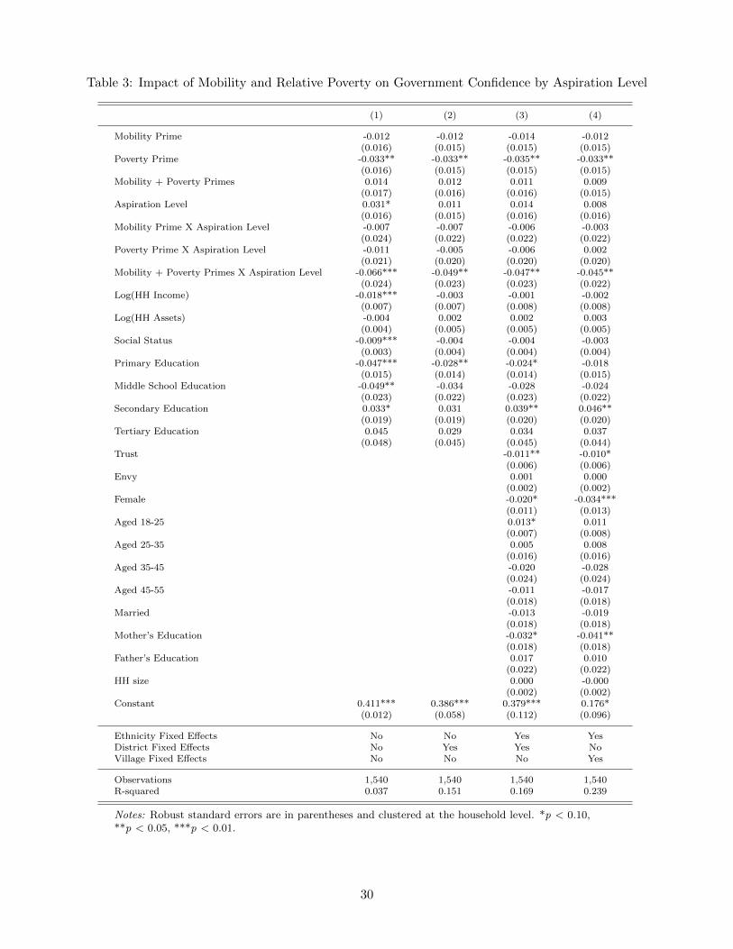
Table 3: Impact of Mobility and Relative Poverty on Government Confidence by Aspiration Level

(1) (2) (3) (4)

Mobility Prime -0.012 -0.012 -0.014 -0.012(0.016) (0.015) (0.015) (0.015)

Poverty Prime -0.033** -0.033** -0.035** -0.033**(0.016) (0.015) (0.015) (0.015)

Mobility + Poverty Primes 0.014 0.012 0.011 0.009(0.017) (0.016) (0.016) (0.015)

Aspiration Level 0.031* 0.011 0.014 0.008(0.016) (0.015) (0.016) (0.016)

Mobility Prime X Aspiration Level -0.007 -0.007 -0.006 -0.003(0.024) (0.022) (0.022) (0.022)

Poverty Prime X Aspiration Level -0.011 -0.005 -0.006 0.002(0.021) (0.020) (0.020) (0.020)

Mobility + Poverty Primes X Aspiration Level -0.066*** -0.049** -0.047** -0.045**(0.024) (0.023) (0.023) (0.022)

Log(HH Income) -0.018*** -0.003 -0.001 -0.002(0.007) (0.007) (0.008) (0.008)

Log(HH Assets) -0.004 0.002 0.002 0.003(0.004) (0.005) (0.005) (0.005)

Social Status -0.009*** -0.004 -0.004 -0.003(0.003) (0.004) (0.004) (0.004)

Primary Education -0.047*** -0.028** -0.024* -0.018(0.015) (0.014) (0.014) (0.015)

Middle School Education -0.049** -0.034 -0.028 -0.024(0.023) (0.022) (0.023) (0.022)

Secondary Education 0.033* 0.031 0.039** 0.046**(0.019) (0.019) (0.020) (0.020)

Tertiary Education 0.045 0.029 0.034 0.037(0.048) (0.045) (0.045) (0.044)

Trust -0.011** -0.010*(0.006) (0.006)

Envy 0.001 0.000(0.002) (0.002)

Female -0.020* -0.034***(0.011) (0.013)

Aged 18-25 0.013* 0.011(0.007) (0.008)

Aged 25-35 0.005 0.008(0.016) (0.016)

Aged 35-45 -0.020 -0.028(0.024) (0.024)

Aged 45-55 -0.011 -0.017(0.018) (0.018)

Married -0.013 -0.019(0.018) (0.018)

Mother’s Education -0.032* -0.041**(0.018) (0.018)

Father’s Education 0.017 0.010(0.022) (0.022)

HH size 0.000 -0.000(0.002) (0.002)

Constant 0.411*** 0.386*** 0.379*** 0.176*(0.012) (0.058) (0.112) (0.096)

Ethnicity Fixed Effects No No Yes YesDistrict Fixed Effects No Yes Yes NoVillage Fixed Effects No No No Yes

Observations 1,540 1,540 1,540 1,540R-squared 0.037 0.151 0.169 0.239

Notes: Robust standard errors are in parentheses and clustered at the household level. *p < 0.10,**p < 0.05, ***p < 0.01.

30

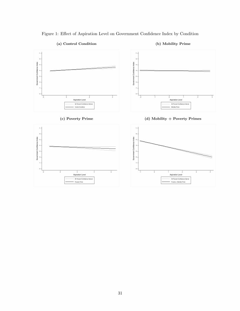
Figure 1: Effect of Aspiration Level on Government Confidence Index by Condition

(a) Control Condition (b) Mobility Prime

0.1

.2.3

.4.5

.6.7

Gov

ernm

ent C

onfid

ence

Inde

x

-2 0 2 4

Aspiration Level

95 Percent Confidence Interval

Control Condition

0.1

.2.3

.4.5

.6.7

Gov

ernm

ent C

onfid

ence

Inde

x

-2 -1 0 1 2 3

Aspiration Level

95 Percent Confidence Interval

Mobility Prime

(c) Poverty Prime (d) Mobility + Poverty Primes

0.1

.2.3

.4.5

.6.7

Gov

ernm

ent C

onfid

ence

Inde

x

-2 0 2 4 6

Aspiration Level

95 Percent Confidence Interval

Poverty Prime

0.1

.2.3

.4.5

.6.7

Gov

ernm

ent C

onfid

ence

Inde

x

-1 0 1 2 3 4

Aspiration Level

95 Percent Confidence Interval

Poverty + Mobility Prime

31

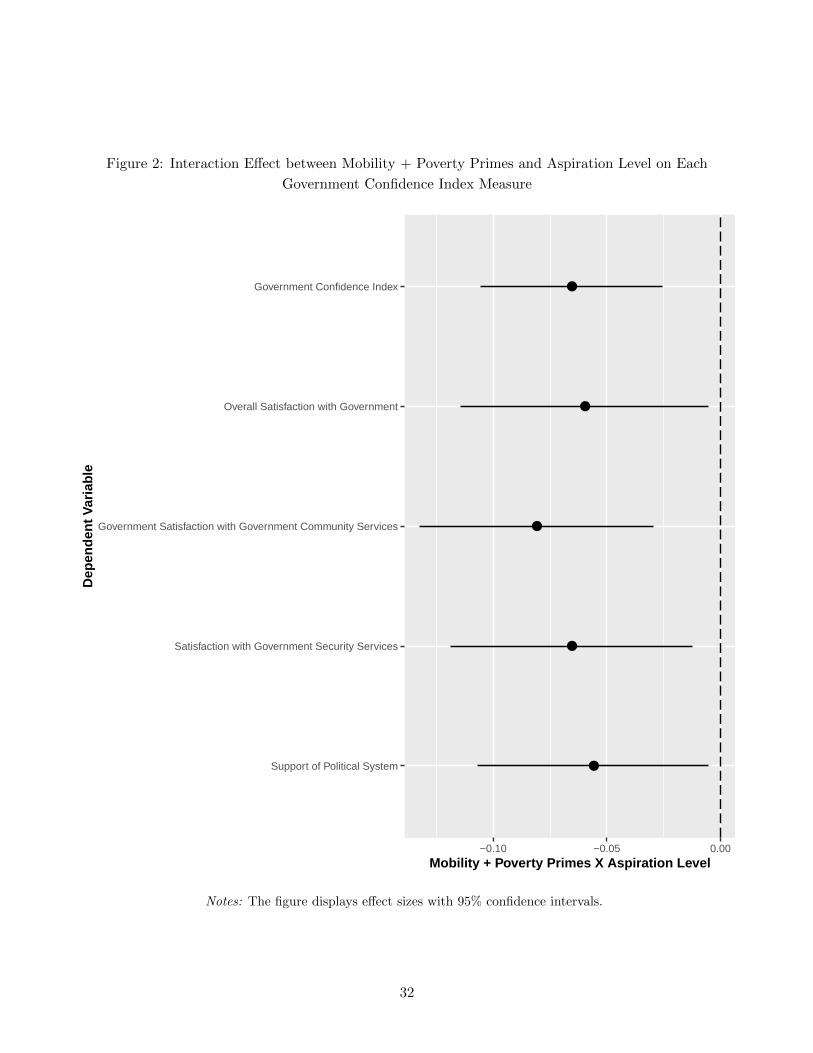
Figure 2: Interaction Effect between Mobility + Poverty Primes and Aspiration Level on Each

Government Confidence Index Measure

●

●

●

●

●

Support of Political System

Satisfaction with Government Security Services

Government Satisfaction with Government Community Services

Overall Satisfaction with Government

Government Confidence Index

−0.10 −0.05 0.00

Mobility + Poverty Primes X Aspiration Level

Dep

ende

nt V

aria

ble

Notes: The figure displays effect sizes with 95% confidence intervals.

32

Online Appendix

Economic Development, Mobility andPolitical Discontent: An Experimental Test

of Tocqueville’s Thesis in Pakistan

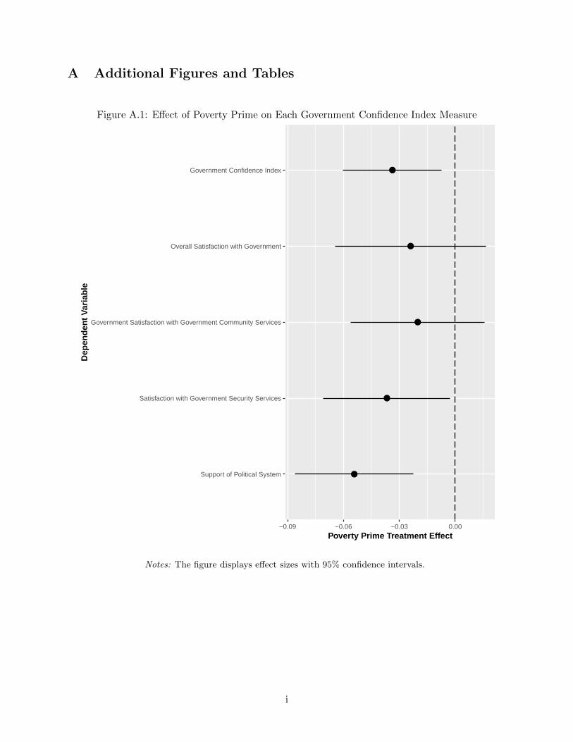
A Additional Figures and Tables

Figure A.1: Effect of Poverty Prime on Each Government Confidence Index Measure

●

●

●

●

●

Support of Political System

Satisfaction with Government Security Services

Government Satisfaction with Government Community Services

Overall Satisfaction with Government

Government Confidence Index

−0.09 −0.06 −0.03 0.00Poverty Prime Treatment Effect

Dep

ende

nt V

aria

ble

Notes: The figure displays effect sizes with 95% confidence intervals.

i

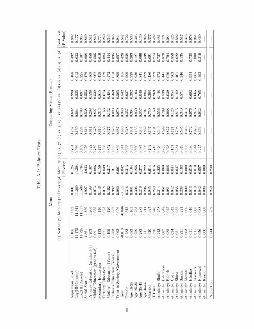
Tab

leA

.1:

Bal

ance

Tes

ts

Mea

nC

om

pari

ng

Mea

ns

(P-v

alu

e)

(1)

Nei

ther

(2)

Mobilit

y(3

)P

over

ty(4

)M

obilit

y(1

)vs.

(2)

(1)

vs.

(3)

(1)

vs.

(4)

(2)

vs.

(3)

(2)

vs.

(4)

(3)

vs.

(4)

Join

tT

est

+P

over

ty(P

-Valu

e)

Asp

irati

on

Lev

el0.1

05

0.0

92

0.0

91

0.1

25

0.7

91

0.7

87

0.6

92

0.9

90

0.4

88

0.4

92

0.8

92

Log(H

HIn

com

e)11.1

75

11.3

11

11.2

69

11.3

04

0.0

36

0.1

60

0.0

64

0.5

35

0.9

13

0.6

33

0.1

77

Log(H

HA

sset

s)11.7

25

11.6

37

11.5

96

11.7

64

0.4

09

0.2

24

0.7

08

0.6

97

0.2

25

0.1

07

0.3

56

Soci

al

Sta

tus

4.8

61

4.8

50

4.9

27

4.9

43

0.9

26

0.6

16

0.5

38

0.5

53

0.4

79

0.9

08

0.8

60

Pri

mary

Educa

tion

(gra

des

1-5

)0.2

03

0.2

06

0.1

88

0.1

67

0.9

22

0.6

11

0.2

08

0.5

38

0.1

69

0.4

50

0.5

11

Mid

dle

Educa

tion

(gra

des

6-8

)0.0

91

0.0

85

0.0

73

0.0

86

0.7

89

0.3

78

0.8

27

0.5

32

0.9

62

0.5

05

0.8

40

Sec

ondary

Educa

tion

0.1

33

0.1

40

0.1

46

0.1

59

0.7

77

0.6

10

0.3

13

0.8

15

0.4

59

0.6

16

0.7

74

Ter

tiary

Educa

tion

0.0

21

0.0

23

0.0

18

0.0

39

0.9

08

0.7

63

0.1

53

0.6

73

0.1

79

0.0

84

0.2

50

Moth

er’s

Educa

tion

(Yea

rs)

0.1

09

0.1

20

0.1

62

0.2

17

0.8

52

0.3

77

0.1

32

0.4

84

0.1

72

0.4

44

0.3

46

Fath

er’s

Educa

tion

(Yea

rs)

0.8

83

0.8

52

0.9

82

1.3

11

0.8

53

0.5

76

0.0

23

0.4

59

0.0

13

0.0

95

0.0

45

Tru

stin

Soci

ety/G

over

nm

ent

0.0

63

0.0

56

0.0

80

0.0

61

0.8

69

0.6

87

0.9

70

0.5

65

0.8

99

0.6

57

0.9

44

Envy

-0.0

18

-0.0

46

-0.0

09

0.0

42

0.6

41

0.8

86

0.3

43

0.5

42

0.1

55

0.4

20

0.5

47

Fem

ale

0.2

83

0.3

13

0.3

16

0.3

13

0.3

53

0.3

18

0.3

57

0.9

37

0.9

99

0.9

38

0.7

22

Age

18-2

50.0

83

0.1

03

0.0

81

0.1

04

0.3

37

0.9

31

0.3

04

0.2

92

0.9

39

0.2

63

0.5

36

Age

25-3

50.2

59

0.2

53

0.3

05

0.2

56

0.8

60

0.1

53

0.9

30

0.1

03

0.9

30

0.1

27

0.3

03

Age

35-4

50.2

83

0.2

83

0.2

19

0.2

77

0.9

87

0.0

44

0.8

57

0.0

40

0.8

41

0.0

66

0.1

30

Age

45-5

50.2

11

0.2

11

0.2

06

0.2

22

0.9

96

0.8

82

0.7

07

0.8

84

0.6

99

0.5

98

0.9

58

Marr

ied

0.9

20

0.9

27

0.9

45

0.9

14

0.7

02

0.1

67

0.7

59

0.3

08

0.4

86

0.0

91

0.3

77

HH

size

6.3

28

6.2

48

6.2

40

6.0

16

0.7

12

0.7

01

0.1

59

0.9

69

0.2

29

0.2

74

0.4

92

ethnic

ity:

Sin

dhi

0.2

43

0.2

58

0.2

14

0.2

25

0.6

20

0.3

49

0.5

56

0.1

48

0.2

73

0.7

27

0.4

81

ethnic

ity:

Pakhto

on

0.0

67

0.0

48

0.0

57

0.0

60

0.2

53

0.5

99

0.7

09

0.5

38

0.4

41

0.8

78

0.7

21

ethnic

ity:

Balo

ch0.0

85

0.0

45

0.0

81

0.0

86

0.0

23

0.8

27

0.9

68

0.0

39

0.0

20

0.7

94

0.0

84

ethnic

ity:

Urd

u0.0

24

0.0

43

0.0

42

0.0

44

0.1

51

0.1

71

0.1

23

0.9

54

0.9

03

0.8

59

0.4

25

ethnic

ity:

Shin

a0.0

51

0.0

35

0.0

55

0.0

47

0.2

84

0.7

98

0.8

15

0.1

82

0.4

01

0.6

22

0.5

92

ethnic

ity:

Sara

iki

0.2

21

0.2

21

0.2

38

0.1

93

0.9

79

0.5

95

0.3

40

0.5

71

0.3

46

0.1

35

0.5

17

ethnic

ity:

Mev

ati

0.0

03

0.0

00

0.0

00

0.0

00

0.3

03

0.3

13

0.3

13

..

.0.3

76

ethnic

ity:

Hin

dko

0.0

11

0.0

10

0.0

13

0.0

10

0.9

30

0.7

62

0.9

76

0.6

92

0.9

54

0.7

38

0.9

78

ethnic

ity:

Marw

ari

0.0

11

0.0

08

0.0

10

0.0

10

0.6

44

0.9

76

0.9

76

0.6

65

0.6

65

1.0

00

0.9

64

ethnic

ity:

Haza

rwal

0.0

56

0.0

38

0.0

42

0.0

57

0.2

25

0.3

64

0.9

32

0.7

65

0.1

92

0.3

19

0.4

69

ethnic

ity:

Kash

mir

i0.0

00

0.0

00

0.0

00

0.0

00

—–

—–

—–

—–

—–

—–

—–

Pro

port

ion

0.2

44

0.2

59

0.2

49

0.2

49

—–

—–

—–

—–

—–

—–

—–

ii

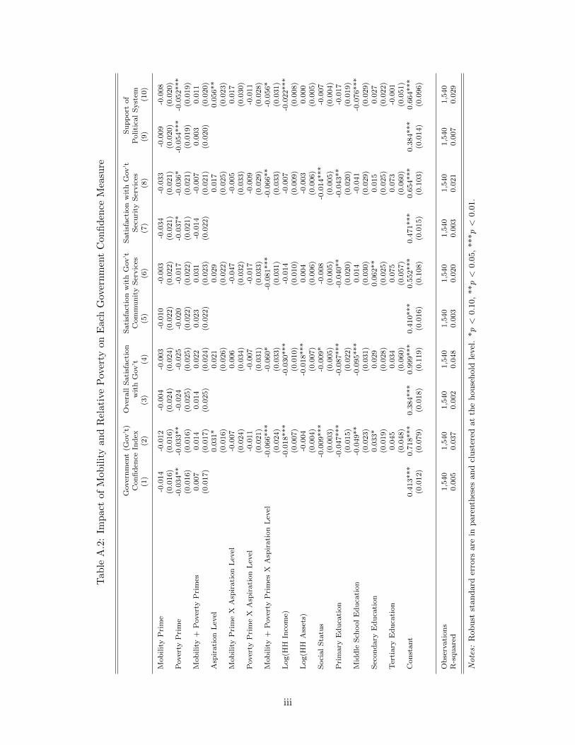
Tab

leA

.2:

Imp

act

ofM

obil

ity

and

Rel

ativ

eP

over

tyon

Eac

hG

over

nm

ent

Con

fid

ence

Mea

sure

Gover

nm

ent

(Gov’t

)O

ver

all

Sati

sfact

ion

Sati

sfact

ion

wit

hG

ov’t

Sati

sfact

ion

wit

hG

ov’t

Su

pp

ort

of

Con

fid

ence

Ind

exw

ith

Gov’t

Com

mu

nit

yS

ervic

esS

ecu

rity

Ser

vic

esP

oliti

cal

Syst

em(1

)(2

)(3

)(4

)(5

)(6

)(7

)(8

)(9

)(1

0)

Mob

ilit

yP

rim

e-0

.014

-0.0

12

-0.0

04

-0.0

03

-0.0

10

-0.0

03

-0.0

34

-0.0

33

-0.0

09

-0.0

08

(0.0

16)

(0.0

16)

(0.0

24)

(0.0

24)

(0.0

22)

(0.0

22)

(0.0

21)

(0.0

21)

(0.0

20)

(0.0

20)

Pover

tyP

rim

e-0

.034**

-0.0

33**

-0.0

24

-0.0

25

-0.0

20

-0.0

17

-0.0

37*

-0.0

36*

-0.0

54***

-0.0

52***

(0.0

16)

(0.0

16)

(0.0

25)

(0.0

25)

(0.0

22)

(0.0

22)

(0.0

21)

(0.0

21)

(0.0

19)

(0.0

19)

Mob

ilit

y+

Pover

tyP

rim

es0.0

07

0.0

14

0.0

14

0.0

22

0.0

23

0.0

31

-0.0

14

-0.0

07

0.0

03

0.0

11

(0.0

17)

(0.0

17)

(0.0

25)

(0.0

24)

(0.0

22)

(0.0

23)

(0.0

22)

(0.0

21)

(0.0

20)

(0.0

20)

Asp

irati

on

Lev

el0.0

31*

0.0

21

0.0

29

0.0

17

0.0

56**

(0.0

16)

(0.0

26)

(0.0

22)

(0.0

25)

(0.0

23)

Mob

ilit

yP

rim

eX

Asp

irati

on

Lev

el-0

.007

0.0

06

-0.0

47

-0.0

05

0.0

17

(0.0

24)

(0.0

34)

(0.0

32)

(0.0

33)

(0.0

30)

Pover

tyP

rim

eX

Asp

irati

on

Lev

el-0

.011

-0.0

07

-0.0

17

-0.0

09

-0.0

11

(0.0

21)

(0.0

31)

(0.0

33)

(0.0

29)

(0.0

28)

Mob

ilit

y+

Pover

tyP

rim

esX

Asp

irati

on

Lev

el-0

.066***

-0.0

60*

-0.0

81***

-0.0

66**

-0.0

56*

(0.0

24)

(0.0

33)

(0.0

31)

(0.0

33)

(0.0

31)

Log(H

HIn

com

e)-0

.018***

-0.0

30***

-0.0

14

-0.0

07

-0.0

22***

(0.0

07)

(0.0

10)

(0.0

10)

(0.0

09)

(0.0

08)

Log(H

HA

sset

s)-0

.004

-0.0

18***

0.0

04

-0.0

03

0.0

00

(0.0

04)

(0.0

07)

(0.0

06)

(0.0

06)

(0.0

05)

Soci

al

Sta

tus

-0.0

09***

-0.0

09*

-0.0

08

-0.0

14***

-0.0

07

(0.0

03)

(0.0

05)

(0.0

05)

(0.0

05)

(0.0

04)

Pri

mary

Ed

uca

tion

-0.0

47***

-0.0

87***

-0.0

40**

-0.0

43**

-0.0

17

(0.0

15)

(0.0

22)

(0.0

20)

(0.0

20)

(0.0

19)

Mid

dle

Sch

ool

Ed

uca

tion

-0.0

49**

-0.0

95***

0.0

14

-0.0

41

-0.0

76***

(0.0

23)

(0.0

31)

(0.0

30)

(0.0

29)

(0.0

29)

Sec

on

dary

Ed

uca

tion

0.0

33*

0.0

29

0.0

62**

0.0

15

0.0

27

(0.0

19)

(0.0

28)

(0.0

25)

(0.0

25)

(0.0

22)

Ter

tiary

Ed

uca

tion

0.0

45

0.0

34

0.0

75

0.0

73

-0.0

01

(0.0

48)

(0.0

60)

(0.0

57)

(0.0

60)

(0.0

51)

Con

stant

0.4

13***

0.7

18***

0.3

84***

0.9

99***

0.4

10***

0.5

52***

0.4

71***

0.6

54***

0.3

84***

0.6

64***

(0.0

12)

(0.0

79)

(0.0

18)

(0.1

19)

(0.0

16)

(0.1

08)

(0.0

15)

(0.1

03)

(0.0

14)

(0.0

96)

Ob

serv

ati

on

s1,5

40

1,5

40

1,5

40

1,5

40

1,5

40

1,5

40

1,5

40

1,5

40

1,5

40

1,5

40

R-s

qu

are

d0.0

05

0.0

37

0.0

02

0.0

48

0.0

03

0.0

20

0.0

03

0.0

21

0.0

07

0.0

29

Notes:

Robust

standard

erro

rsare

inpare

nth

eses

and

clust

ered

at

the

house

hold

level

.*p<

0.1

0,

**p<

0.0

5,

***p<

0.0

1.

iii

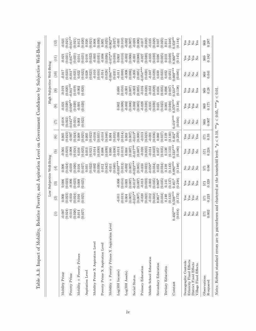
Tab

leA

.3:

Imp

act

ofM

obil

ity,

Rel

ativ

eP

over

ty,

and

Asp

irat

ion

Lev

elon

Gov

ern

men

tC

onfi

den

ceby

Sub

ject

ive

Wel

l-B

ein

g

Low

Su

bje

ctiv

eW

ell-

Bei

ng

Hig

hS

ub

ject

ive

Wel

l-B

ein

g

(1)

(2)

(3)

(4)

(5)

(6)

(7)

(8)

(9)

(10)

(11)

(12)

Mob

ilit

yP

rim

e-0

.007

0.0

00

0.0

06

0.0

06

-0.0

01

0.0

05

-0.0

18

-0.0

21

-0.0

19

-0.0

17

-0.0

21

-0.0

21

(0.0

24)

(0.0

23)

(0.0

23)

(0.0

24)

(0.0

23)

(0.0

23)

(0.0

22)

(0.0

20)

(0.0

20)

(0.0

23)

(0.0

21)

(0.0

21)

Pover

tyP

rim

e-0

.014

-0.0

10

-0.0

06

-0.0

10

-0.0

08

-0.0

07

-0.0

45**

-0.0

48**

-0.0

41**

-0.0

41*

-0.0

47**

-0.0

41**

(0.0

26)

(0.0

24)

(0.0

23)

(0.0

26)

(0.0

24)

(0.0

24)

(0.0

21)

(0.0

20)

(0.0

19)

(0.0

21)

(0.0

21)

(0.0

21)

Mob

ilit

y+

Pover

tyP

rim

es0.0

14

0.0

16

0.0

09

0.0

16

0.0

16

0.0

09

0.0

03

-0.0

01

-0.0

02

0.0

22

0.0

14

0.0

12

(0.0

27)

(0.0

25)

(0.0

25)

(0.0

27)

(0.0

25)

(0.0

25)

(0.0

22)

(0.0

20)

(0.0

20)

(0.0

22)

(0.0

21)

(0.0

20)

Asp

irati

on

Lev

el0.0

31

0.0

13

0.0

05

0.0

28

0.0

16

0.0

20

(0.0

22)

(0.0

21)

(0.0

22)

(0.0

23)

(0.0

22)

(0.0

21)

Mob

ilit

yP

rim

eX

Asp

irati

on

Lev

el-0

.002

-0.0

14

-0.0

16

-0.0

10

-0.0

03

0.0

08

(0.0

30)

(0.0

30)

(0.0

31)

(0.0

34)

(0.0

31)

(0.0

30)

Pover

tyP

rim

eX

Asp

irati

on

Lev

el0.0

12

0.0

08

-0.0

14

-0.0

14

-0.0

08

0.0

05

(0.0

42)

(0.0

39)

(0.0

40)

(0.0

28)

(0.0

26)

(0.0

25)

Mob

ilit

y+

Pover

tyP

rim

esX

Asp

irati

on

Lev

el-0

.011

0.0

00

0.0

04

-0.0

94***

-0.0

72**

-0.0

62**

(0.0

40)

(0.0

36)

(0.0

33)

(0.0

31)

(0.0

30)

(0.0

27)

Log(H

HIn

com

e)-0

.011

-0.0

06

-0.0

33***

-0.0

13

-0.0

06

0.0

02

0.0

00

-0.0

11

0.0

03

-0.0

01

(0.0

13)

(0.0

14)

(0.0

13)

(0.0

13)

(0.0

14)

(0.0

09)

(0.0

10)

(0.0

09)

(0.0

10)

(0.0

10)

Log(H

HA

sset

s)0.0

04

0.0

03

-0.0

02

0.0

04

0.0

03

-0.0

02

-0.0

01

-0.0

08

-0.0

02

-0.0

02

(0.0

07)

(0.0

07)

(0.0

07)

(0.0

07)

(0.0

07)

(0.0

06)

(0.0

07)

(0.0

06)

(0.0

06)

(0.0

07)

Soci

al

Sta

tus

-0.0

15**

-0.0

13*

-0.0

23***

-0.0

17**

-0.0

13*

-0.0

02

-0.0

03

-0.0

05

-0.0

01

-0.0

03

(0.0

07)

(0.0

07)

(0.0

05)

(0.0

07)

(0.0

08)

(0.0

05)

(0.0

05)

(0.0

05)

(0.0

06)

(0.0

06)

Pri

mary

Ed

uca

tion

-0.0

20

-0.0

13

-0.0

34

-0.0

20

-0.0

13

-0.0

29

-0.0

16

-0.0

54***

-0.0

27

-0.0

17

(0.0

22)

(0.0

23)

(0.0

22)

(0.0

23)

(0.0

23)

(0.0

20)

(0.0

20)

(0.0

20)

(0.0

20)

(0.0

20)

Mid

dle

Sch

ool

Ed

uca

tion

-0.0

12

-0.0

03

-0.0

58*

-0.0

14

-0.0

01

-0.0

35

-0.0

33

-0.0

47

-0.0

33

-0.0

35

(0.0

32)

(0.0

35)

(0.0

34)

(0.0

33)

(0.0

36)

(0.0

30)

(0.0

29)

(0.0

29)

(0.0

30)

(0.0

29)

Sec

on

dary

Ed

uca

tion

0.0

61*

0.0

60*

0.0

32

0.0

57

0.0

60

0.0

21

0.0

34

0.0

30

0.0

26

0.0

37

(0.0

34)

(0.0

35)

(0.0

34)

(0.0

35)

(0.0

37)

(0.0

25)

(0.0

25)

(0.0

23)

(0.0

25)

(0.0

25)

Ter

tiary

Ed

uca

tion

0.1

40

0.1

41

0.1

39

0.1

36

0.1

39

0.0

01

0.0

06

0.0

32

0.0

10

0.0

11

(0.1

32)

(0.1

37)

(0.1

43)

(0.1

33)

(0.1

40)

(0.0

48)

(0.0

47)

(0.0

51)

(0.0

49)

(0.0

48)

Con

stant

0.4

02***

0.5

08***

0.4

61*

0.8

80***

0.5

33***

0.4

62*

0.4

19***

0.3

79***

0.3

24**

0.6

69***

0.3

60**

0.3

59**

(0.0

18)

(0.1

72)

(0.2

48)

(0.1

48)

(0.1

80)

(0.2

59)

(0.0

16)

(0.1

38)

(0.1

38)

(0.0

95)

(0.1

45)

(0.1

44)

Dem

ogra

ph

icC

ontr

ols

No

Yes

Yes

No

Yes

Yes

No

Yes

Yes

No

Yes

Yes

Eth

nic

ity

Fix

edE

ffec

tsN

oY

esY

esN

oY

esY

esN

oY

esY

esN

oY

esY

esD

istr

ict

Fix

edE

ffec

tsN

oY

esN

oN

oY

esN

oN

oY

esN

oN

oY

esN

oV

illa

ge

Fix

edE

ffec

tsN

oN

oY

esN

oN

oY

esN

oN

oY

esN

oN

oY

es

Ob

serv

ati

on

s571

571

571

571

571

571

969

969

969

969

969

969

R-s

qu

are

d0.0

02

0.2

23

0.3

29

0.0

60.2

24

0.3

30.0

07

0.1

75

0.2

80.0

41

0.1

82

0.2

87

Notes:

Robust

standard

erro

rsare

inpare

nth

eses

and

clust

ered

at

the

house

hold

level

.*p<

0.1

0,

**p<

0.0

5,

***p<

0.0

1.

iv

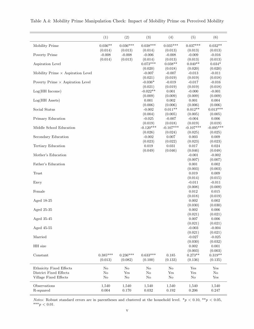
Table A.4: Mobility Prime Manipulation Check: Impact of Mobility Prime on Perceived Mobility

(1) (2) (3) (4) (5) (6)

Mobility Prime 0.036** 0.036*** 0.038*** 0.035*** 0.037*** 0.032**(0.014) (0.013) (0.014) (0.013) (0.013) (0.013)

Poverty Prime -0.008 -0.008 -0.006 -0.008 -0.009 -0.016(0.014) (0.013) (0.014) (0.013) (0.013) (0.013)

Aspiration Level 0.073*** 0.038** 0.040** 0.034*(0.020) (0.018) (0.020) (0.020)

Mobility Prime × Aspiration Level -0.007 -0.007 -0.013 -0.011(0.021) (0.019) (0.019) (0.018)

Poverty Prime × Aspiration Level -0.036* -0.019 -0.017 -0.016(0.021) (0.019) (0.019) (0.018)

Log(HH Income) -0.022** 0.001 -0.000 -0.001(0.009) (0.009) (0.009) (0.009)

Log(HH Assets) 0.001 0.002 0.001 0.004(0.006) (0.006) (0.006) (0.006)

Social Status -0.002 0.011** 0.012** 0.013***(0.004) (0.005) (0.005) (0.005)

Primary Education -0.025 -0.007 -0.004 0.006(0.019) (0.018) (0.019) (0.019)

Middle School Education -0.120*** -0.107*** -0.107*** -0.095***(0.026) (0.024) (0.025) (0.025)

Secondary Education -0.002 0.007 0.003 0.009(0.023) (0.022) (0.023) (0.023)

Tertiary Education 0.019 0.031 0.017 0.024(0.049) (0.046) (0.046) (0.048)

Mother’s Education -0.001 -0.002(0.007) (0.007)

Father’s Education 0.001 0.002(0.003) (0.003)

Trust 0.019 0.009(0.014) (0.015)

Envy -0.011 -0.011(0.008) (0.009)

Female 0.012 0.015(0.018) (0.019)

Aged 18-25 0.002 0.002(0.030) (0.030)

Aged 25-35 0.002 0.006(0.021) (0.021)

Aged 35-45 0.007 0.006(0.021) (0.021)

Aged 45-55 -0.003 -0.004(0.021) (0.021)

Married -0.027 -0.025(0.030) (0.032)

HH size 0.002 0.001(0.003) (0.003)

Constant 0.385*** 0.236*** 0.633*** 0.185 0.273** 0.319**(0.013) (0.082) (0.100) (0.133) (0.136) (0.135)

Ethnicity Fixed Effects No No No No Yes YesDistrict Fixed Effects No Yes No Yes Yes NoVillage Fixed Effects No No No No No Yes

Observations 1,540 1,540 1,540 1,540 1,540 1,540R-squared 0.004 0.170 0.032 0.192 0.206 0.247

Notes: Robust standard errors are in parentheses and clustered at the household level. *p < 0.10, **p < 0.05,***p < 0.01.

v

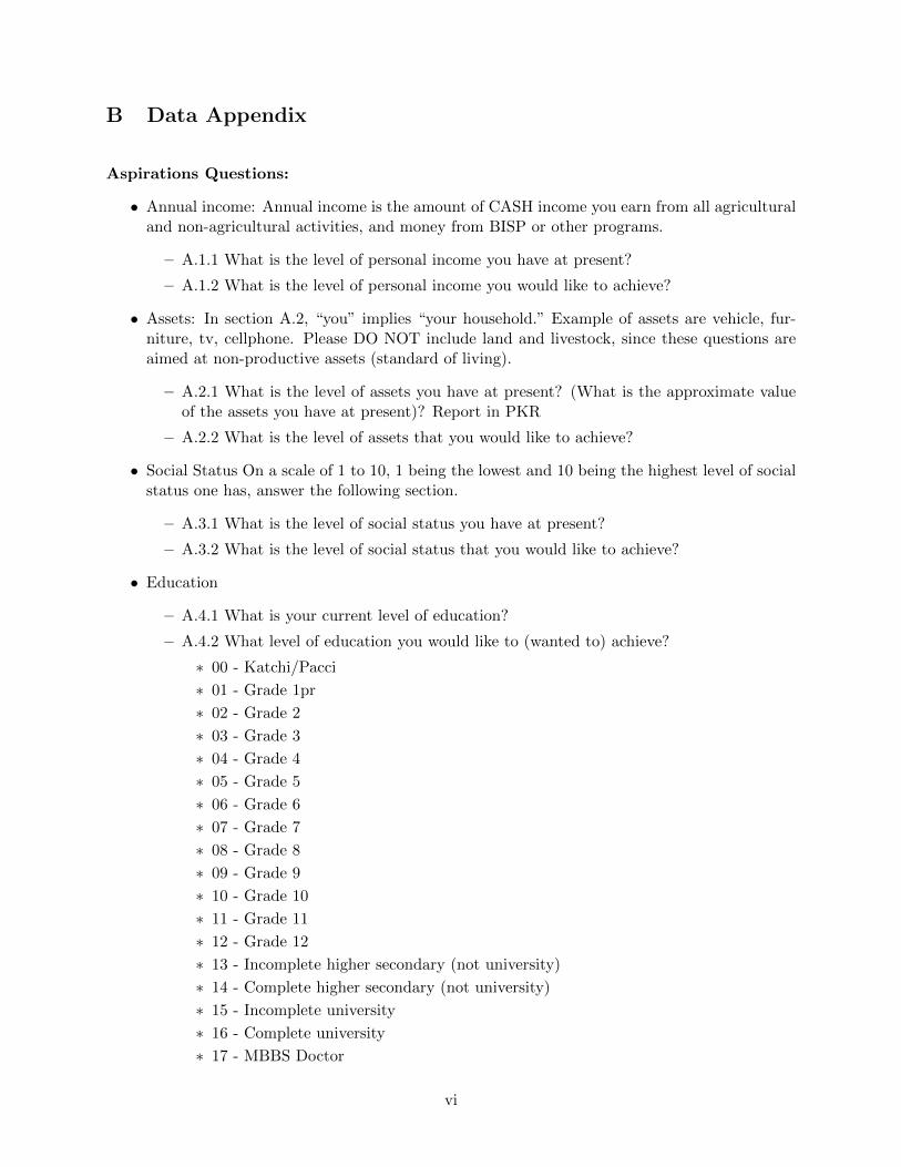
B Data Appendix

Aspirations Questions:

• Annual income: Annual income is the amount of CASH income you earn from all agriculturaland non-agricultural activities, and money from BISP or other programs.

– A.1.1 What is the level of personal income you have at present?

– A.1.2 What is the level of personal income you would like to achieve?

• Assets: In section A.2, “you” implies “your household.” Example of assets are vehicle, fur-niture, tv, cellphone. Please DO NOT include land and livestock, since these questions areaimed at non-productive assets (standard of living).

– A.2.1 What is the level of assets you have at present? (What is the approximate valueof the assets you have at present)? Report in PKR

– A.2.2 What is the level of assets that you would like to achieve?

• Social Status On a scale of 1 to 10, 1 being the lowest and 10 being the highest level of socialstatus one has, answer the following section.

– A.3.1 What is the level of social status you have at present?

– A.3.2 What is the level of social status that you would like to achieve?

• Education

– A.4.1 What is your current level of education?

– A.4.2 What level of education you would like to (wanted to) achieve?

∗ 00 - Katchi/Pacci

∗ 01 - Grade 1pr

∗ 02 - Grade 2

∗ 03 - Grade 3

∗ 04 - Grade 4

∗ 05 - Grade 5

∗ 06 - Grade 6

∗ 07 - Grade 7

∗ 08 - Grade 8

∗ 09 - Grade 9

∗ 10 - Grade 10

∗ 11 - Grade 11

∗ 12 - Grade 12

∗ 13 - Incomplete higher secondary (not university)

∗ 14 - Complete higher secondary (not university)

∗ 15 - Incomplete university

∗ 16 - Complete university

∗ 17 - MBBS Doctor

vi

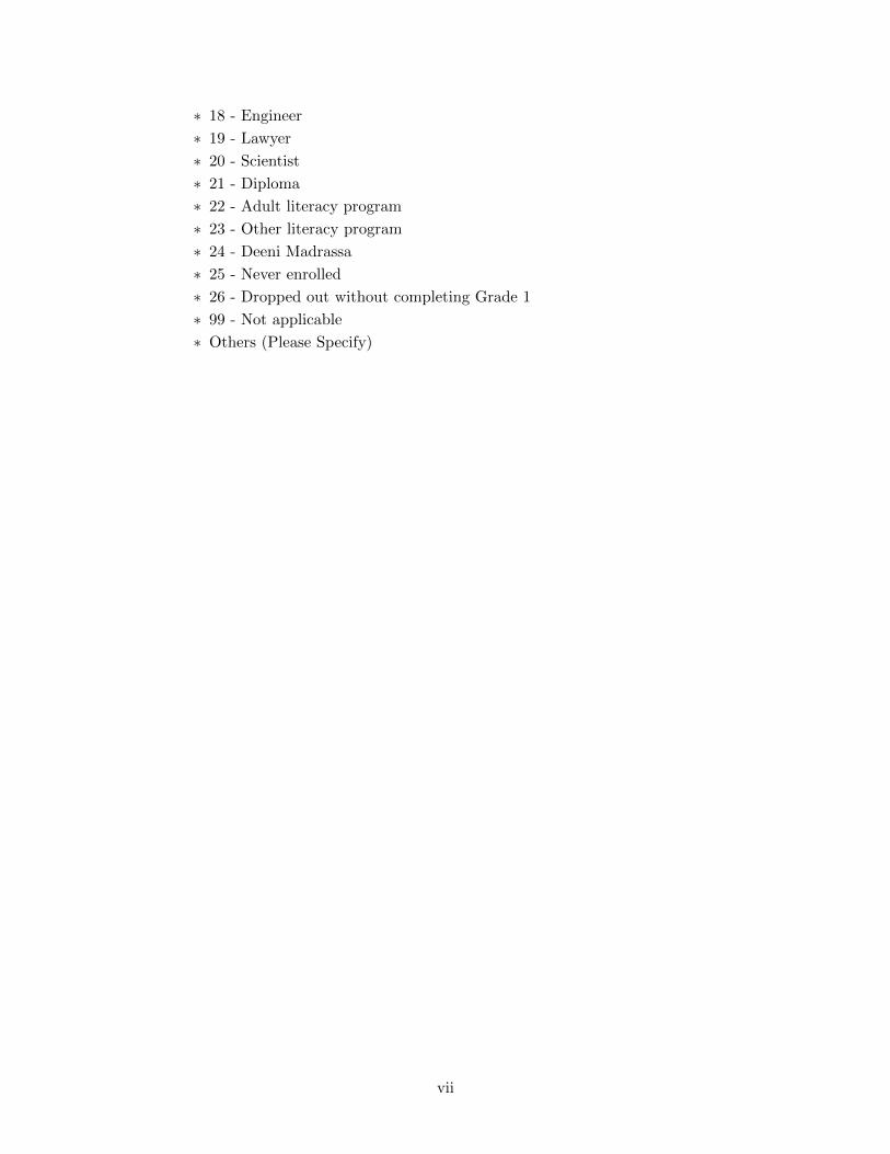
∗ 18 - Engineer

∗ 19 - Lawyer

∗ 20 - Scientist

∗ 21 - Diploma

∗ 22 - Adult literacy program

∗ 23 - Other literacy program

∗ 24 - Deeni Madrassa

∗ 25 - Never enrolled

∗ 26 - Dropped out without completing Grade 1

∗ 99 - Not applicable

∗ Others (Please Specify)

vii