Department of EconomicsWorking Paper No. 215

Economic Development and Forest Cover: Evidence from Satellite Data

Jesús Crespo Cuaresma Olha Danylo Steffen Fritz Ian McCallum Michael Obersteiner Linda See

January 2016

1

Economic Development and Forest Cover: Evidence from Satellite Data*

Jesús Crespo CuaresmaVienna University of Economics and Business, Wittgenstein Centre for Demography and Human Capital, International Institute for Applied Systems Analysis, Austrian Institute of Economic Research

Olha Danylo International Institute for Applied Systems Analysis

Steffen Fritz International Institute for Applied Systems Analysis

Ian McCallum International Institute for Applied Systems Analysis

Michael Obersteiner International Institute for Applied Systems Analysis

Linda See International Institute for Applied Systems Analysis

Abstract

We use satellite data on forest cover along national borders in order to study the determinants of deforestation differences across countries. We combine the forest cover information with data on homogeneous response units, which allow us to control for cross-country geoclimatic differences when assessing the drivers of deforestation. Income per capita appears to be the most robust determinant of differences in cross-border forest cover and our results present evidence of the existence of decreasing effects of income on forest cover as economic development progresses.

Keywords: deforestation, environmental Kuznets curve, national borders

JEL Classifications: Q23, Q56

*Corresponding author: Jesus Crespo Cuaresma (jcrespo@wu.ac.at). The authors are indebted to Ester Blanco, Bill Butz, Stephan Klasen, James R. Vreeland, Konstantin Wacker and the participants in research seminars at the University of Innsbruck, at the University of Göttingen and the Vienna University of Economics and Business for helpful comments on an earlier version of this paper. Research assistance by Franziska Albrecht is gratefully acknowledged. The projects GEOCARBON (FP7 283080) and REDD-PAC (http://www.redd-pac.org/) supported this study.

2

The substantial increase in human activity over the last century has resulted in forest decline, in particular in the tropical areas of the world, either through deforestation, i.e. depletion of the tree crown cover to less than 10 percent, or degradation, i.e. negative structural or functional changes to the forest that reduce the quality through over-exploitation, repeated fires or disease (Lewis et al., 2015; Trumbore et al., 2015). Some of the key research in this area has focused on the precise assessment of deforestation rates (Achard et al., 2004; Lepers et al., 2005), while another key challenge has been to understand the drivers and underlying causes of deforestation (Geist and Lambin, 2002; Andam et al., 2008; Macedo et al., 2012). Some of the causes put forth in the literature include increases in overall population (Amelung and Diehl, 1992; Cropper and Griffiths, 1994), specifically in urban areas (DeFries et al., 2010), agricultural practices such as shifting cultivation (Ranjan and Upadhyay, 1999), transport costs and government policies (Pfaff, 1999) and agricultural trade (DeFries et al., 2010).

The empirical support of the hypothesis of an environmental Kuznets curve for deforestation has until now proven elusive, with studies finding evidence for and against its existence depending on the dataset, estimation method and sample used (see Koop and Tole, 1999; Bhattarai and Hammig, 2001; Erhardt-Martinez et al. 2002 or Culas, 2012). In addition, forest statistics have been traditionally plagued by accounting and reporting errors (Grainger and Obersteiner, 2011). In this contribution we provide evidence on the relationship between economic development and forest cover using a satellite-based dataset of forest cover (Hansen et al., 2003) across national borders worldwide for the year 2005. We contribute to the literature by exploiting the discontinuities created by national borders as a natural experiment (see for example Pinkovskiy, 2013, for a similar research design aimed at measuring the effect of institutions on economic development). Furthermore we use a Homogeneous Response Units (HRU) layer (Havlik et al., 2010) in order to ensure comparability of geoclimatic characteristics across countries. These sources allow us to construct a measure of relative forest cover for each pair of neighboring countries, using a buffer of 50 kilometers on both sides of each national border.

The dataset we construct allows us to identify country-specific socioeconomic determinants of differences in forest cover across countries while keeping environmental factors as constant as possible. We estimate regression models for the global sample covering all borders of the world for which data are available. Following Cropper and Griffiths (1994), forest cover differences are assumed to depend on the relative income per capita of the countries on both sides of the border, their growth rate of income per capita, population growth and rural population density. We include in our specification the difference in squared income per capita levels in order to test for a U-shape relationship between the level of development of a country and forest cover at the border and also entertain threshold regressions in order to allow for nonlinearities in the deforestation Kuznets curve. Our results support the existence of a leveling out of the relationship between forest cover and income per capita with a turning point which is located roughly at a per capita income level of 5,500 PPP-adjusted 2005 international dollars, corresponding approximately to the per capita income of Guatemala.

3

I. Measuring Forest cover Across National Borders

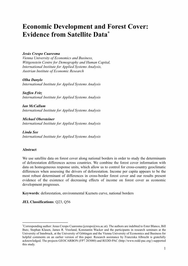
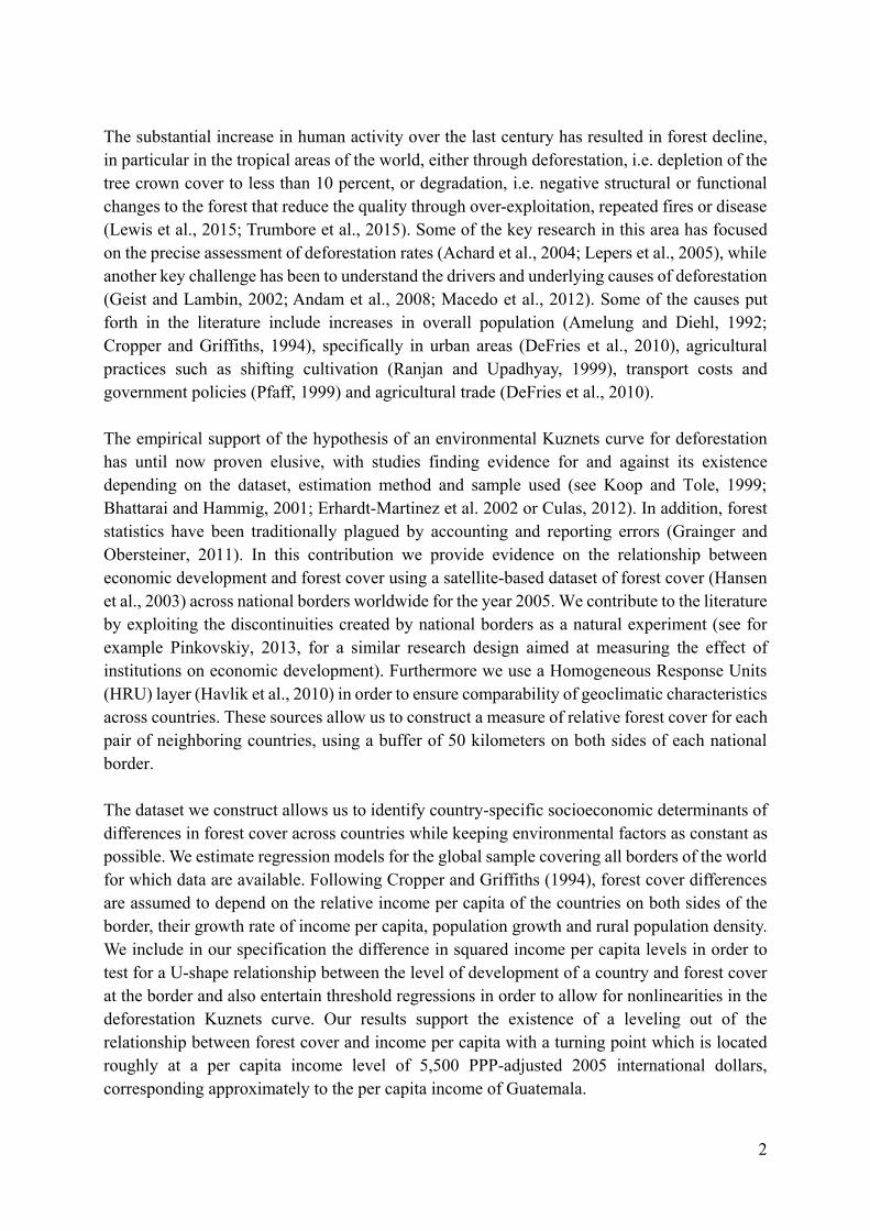
National borders play the role of a natural experiment in our assessment of the determinants of forest cover differences across countries of the world. Once differences in altitude, slope and soil composition between the two sides of a border are taken into account (via HRUs), our identification strategy relies on the fact that differences in forest cover between the two countries that the border separates are determined by differences in socioeconomic and institutional characteristics between the two nations. We combine the forest cover data derived from Hansen (2003) with HRUs, which are defined based on classifications of altitude (five classes: 0 - 300 m, 300 - 600 m, 600 - 1100 m, 1100 - 2500 m and more than 2500 m), slope (seven classes: 0° - 3°, 3° - 6°, 6° - 10°, 10° - 15°, 15° - 30°, 30° - 50° and more than 50°) and soil composition (five classes: sandy, loamy, clay, stony and peat). Figure 1 presents the forest cover estimates based on HRUs along a 50 km buffer on both sides of four selected borders: Brazil-Bolivia, Afghanistan-Pakistan, Laos-Thailand and Angola-Democratic Republic of Congo. In order to grasp the differences in forest cover existing across borders worldwide, Figure 2 presents the ratio of forest cover for the HRU with the largest area on both sides of the border, which we label the Cross-Border Deforestation Index (CBDI). In order to ensure that the forest cover difference is not driven by small areas, the CBDI is obtained using the maximum area of HRU shared by bordering countries, requiring that a minimum of 500 km2 of the HRU area is present on each side of the border and that at least one of the two sides of the border contains a minimum forest coverage of 20% (see the Appendix for more details on the remote sensing methods employed and a comparison with Hansen, 2013).

In Figure 2, borders without color correspond to terrain where the forest cover is less than 20% (e.g. deserts), or where the conditions for computing the CBDI were not met (i.e. the cross-border maximal HRU area is too small). The map shows high values of the index in most continents. The strong differences in forest cover between Haiti and the Dominican Republic are picked up very clearly by the method and large vegetation differentials are also observable between Belize and Guatemala, El Salvador and its neighboring countries, as well as Brazil and its southern neighbors. Similar differences are observed in Africa, for instance between Sudan and Ethiopia and between Burundi or Rwanda and the Democratic Republic of Congo. In Asia, stark cross-border differences in forest cover are observable in particular between China and many of its neighboring nations.

4

Figure 1: Forest cover along identical homogeneous response units for Bolivia-Brazil, Laos-Thailand; Afghanistan-Pakistan and Angola-Democratic Republic of Congo

Figure 2: Cross-Border Deforestation Index for all national borders for which data are available

5

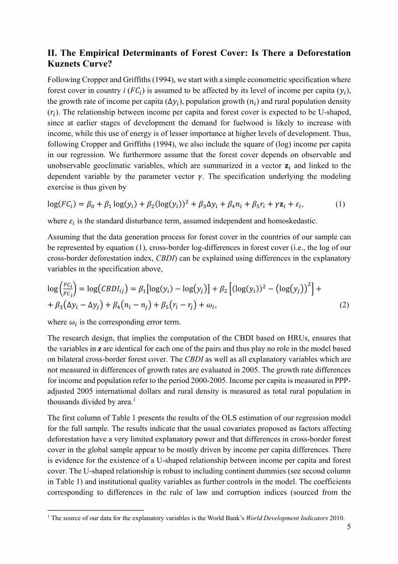
II. The Empirical Determinants of Forest Cover: Is There a Deforestation Kuznets Curve? Following Cropper and Griffiths (1994), we start with a simple econometric specification where forest cover in country i () is assumed to be affected by its level of income per capita (), the growth rate of income per capita (∆), population growth () and rural population density (). The relationship between income per capita and forest cover is expected to be U-shaped, since at earlier stages of development the demand for fuelwood is likely to increase with income, while this use of energy is of lesser importance at higher levels of development. Thus, following Cropper and Griffiths (1994), we also include the square of (log) income per capita in our regression. We furthermore assume that the forest cover depends on observable and unobservable geoclimatic variables, which are summarized in a vector and linked to the dependent variable by the parameter vector . The specification underlying the modeling exercise is thus given by

log log log ∆ , (1)

where is the standard disturbance term, assumed independent and homoskedastic.

Assuming that the data generation process for forest cover in the countries of our sample can be represented by equation (1), cross-border log-differences in forest cover (i.e., the log of our cross-border deforestation index, CBDI) can be explained using differences in the explanatory variables in the specification above,

log log log log log log ∆ ∆ , (2)

where is the corresponding error term.

The research design, that implies the computation of the CBDI based on HRUs, ensures that the variables in z are identical for each one of the pairs and thus play no role in the model based on bilateral cross-border forest cover. The CBDI as well as all explanatory variables which are not measured in differences of growth rates are evaluated in 2005. The growth rate differences for income and population refer to the period 2000-2005. Income per capita is measured in PPP-adjusted 2005 international dollars and rural density is measured as total rural population in thousands divided by area.1

The first column of Table 1 presents the results of the OLS estimation of our regression model for the full sample. The results indicate that the usual covariates proposed as factors affecting deforestation have a very limited explanatory power and that differences in cross-border forest cover in the global sample appear to be mostly driven by income per capita differences. There is evidence for the existence of a U-shaped relationship between income per capita and forest cover. The U-shaped relationship is robust to including continent dummies (see second column in Table 1) and institutional quality variables as further controls in the model. The coefficients corresponding to differences in the rule of law and corruption indices (sourced from the

1 The source of our data for the explanatory variables is the World Bank’s World Development Indicators 2010.

6

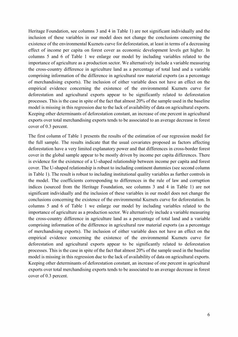
Heritage Foundation, see columns 3 and 4 in Table 1) are not significant individually and the inclusion of these variables in our model does not change the conclusions concerning the existence of the environmental Kuznets curve for deforestation, at least in terms of a decreasing effect of income per capita on forest cover as economic development levels get higher. In columns 5 and 6 of Table 1 we enlarge our model by including variables related to the importance of agriculture as a production sector. We alternatively include a variable measuring the cross-country difference in agriculture land as a percentage of total land and a variable comprising information of the difference in agricultural raw material exports (as a percentage of merchandising exports). The inclusion of either variable does not have an effect on the empirical evidence concerning the existence of the environmental Kuznets curve for deforestation and agricultural exports appear to be significantly related to deforestation processes. This is the case in spite of the fact that almost 20% of the sample used in the baseline model is missing in this regression due to the lack of availability of data on agricultural exports. Keeping other determinants of deforestation constant, an increase of one percent in agricultural exports over total merchandising exports tends to be associated to an average decrease in forest cover of 0.3 percent.

The first column of Table 1 presents the results of the estimation of our regression model for the full sample. The results indicate that the usual covariates proposed as factors affecting deforestation have a very limited explanatory power and that differences in cross-border forest cover in the global sample appear to be mostly driven by income per capita differences. There is evidence for the existence of a U-shaped relationship between income per capita and forest cover. The U-shaped relationship is robust to including continent dummies (see second column in Table 1). The result is robust to including institutional quality variables as further controls in the model. The coefficients corresponding to differences in the rule of law and corruption indices (sourced from the Heritage Foundation, see columns 3 and 4 in Table 1) are not significant individually and the inclusion of these variables in our model does not change the conclusions concerning the existence of the environmental Kuznets curve for deforestation. In columns 5 and 6 of Table 1 we enlarge our model by including variables related to the importance of agriculture as a production sector. We alternatively include a variable measuring the cross-country difference in agriculture land as a percentage of total land and a variable comprising information of the difference in agricultural raw material exports (as a percentage of merchandising exports). The inclusion of either variable does not have an effect on the empirical evidence concerning the existence of the environmental Kuznets curve for deforestation and agricultural exports appear to be significantly related to deforestation processes. This is the case in spite of the fact that almost 20% of the sample used in the baseline model is missing in this regression due to the lack of availability of data on agricultural exports. Keeping other determinants of deforestation constant, an increase of one percent in agricultural exports over total merchandising exports tends to be associated to an average decrease in forest cover of 0.3 percent.

7

(1) (2) (3) (4) (5) (6)

Income per capita -0.441** -0.448** -0.469** -0.473** -0.352* -0.700**

[0.179] [0.178] [0.182] [0.187] [0.186] [0.321]

(Income per capita)2 0.0256** 0.0261** 0.0281** 0.0283** 0.0202* 0.0400**

[0.0113] [0.0112] [0.0116] [0.0121] [0.0116] [0.0193]

Income growth 0.0484 0.0104 0.000278 -0.00343 0.0225 -0.0672

[0.0510] [0.0494] [0.0492] [0.0510] [0.0482] [0.164]

Population growth 0.259 0.319 0.354 0.333 0.237 -0.11

[0.609] [0.573] [0.568] [0.573] [0.587] [0.710]

Rural pop. density -0.34 -0.344 -0.322 -0.336 -0.161 0.0106

[0.327] [0.344] [0.342] [0.344] [0.389] [0.466]

Rule of law -0.0234

[0.0240]

Corruption -0.0237

[0.0260]

Agricultural land -0.125

[0.0942]

Agric. raw material exports -0.377**

[0.147]

Continent dummies No Yes Yes Yes Yes Yes

Observations 189 189 189 189 183 154

R-squared 0.046 0.077 0.080 0.080 0.083 0.066

Robust standard errors in parenthesis.*(**) stands for significance at the 10%(5%) level. Dependent variable is the (log) cross-border deforestation index (CBDI) in 2005. Income per capiita refers to the log of GDP per capita in 2005, income growth Is the growth of GDP per capita 2000-2005 (source: World Development Indicators 2010). Rule of law and corruption indices are sourced from the Heritage Foundation.

Table 1: Estimation results, determinants of bilateral forest cover differences

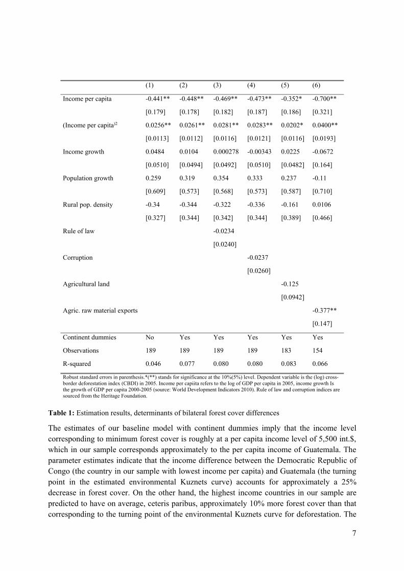
The estimates of our baseline model with continent dummies imply that the income level corresponding to minimum forest cover is roughly at a per capita income level of 5,500 int.$, which in our sample corresponds approximately to the per capita income of Guatemala. The parameter estimates indicate that the income difference between the Democratic Republic of Congo (the country in our sample with lowest income per capita) and Guatemala (the turning point in the estimated environmental Kuznets curve) accounts for approximately a 25% decrease in forest cover. On the other hand, the highest income countries in our sample are predicted to have on average, ceteris paribus, approximately 10% more forest cover than that corresponding to the turning point of the environmental Kuznets curve for deforestation. The

8

estimate of our transition threshold is in line with previous results in the literature. In particular, it is similar to the transition value found in Kauppi et al. (2006), whose estimate is based exclusively on comparing the significance of changes in forest cover.

The fitted environmental Kuznets curve for deforestation, which is implied from the parameter estimates for the baseline model, is depicted in Figure 2. The dispersion of our estimated parameters and the range of observed income values imply that there is only weak evidence concerning the upward-sloping effect of income on forest cover (i.e. the reforestation part of the environmental Kuznets curve). We performed an additional robustness check by estimating models with a piecewise-linear link between income and forest cover, instead of a quadratic one. Such class of models allows for more flexibility in terms of accounting for an asymmetric response of deforestation to income depending on the level of development of the country. We estimate the income threshold which triggers the change in the slope of the deforestation Kuznets curve using the method put forward by Hansen (2000). The estimation results in a threshold estimate of roughly 9200 international dollars, which corresponds to the 64th

percentile of our income per capita sample. The estimate of the slope of the relationship between income and forest cover for countries whose income per capita is below the threshold is -0.038, with a standard deviation of 0.02 and the estimate for the rest of the sample is -0.026, with a standard deviation of 0.024. The threshold model thus supports an environmental Kuznets curve for deforestation which does not present a reverting trend for richer economies. Instead, the estimation results indicate that the deforestation effect of economic development disappears (but does not revert) as the income level increases.2

Figure 2: Estimated relationship between income per capita and forest cover

2 Grossman and Krueger (1995) also present evidence of environmental Kuznets curves whose reversal is not significant for other measures of air and water pollution.

9

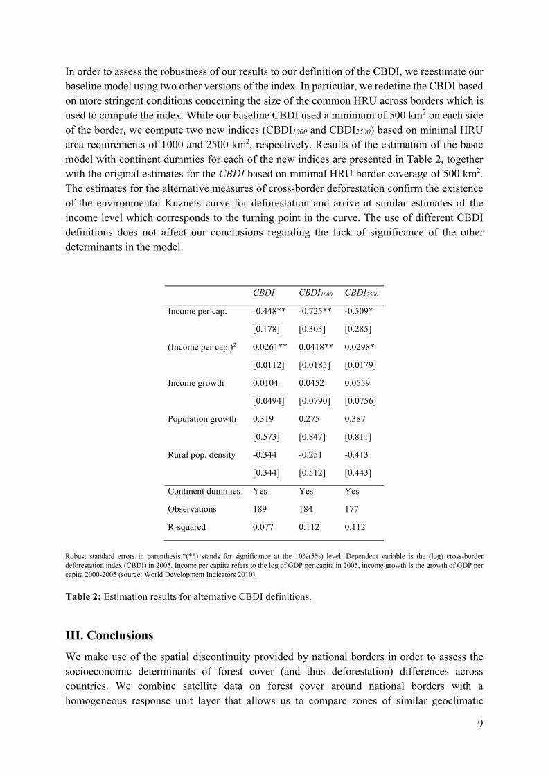
In order to assess the robustness of our results to our definition of the CBDI, we reestimate our baseline model using two other versions of the index. In particular, we redefine the CBDI based on more stringent conditions concerning the size of the common HRU across borders which is used to compute the index. While our baseline CBDI used a minimum of 500 km2 on each side of the border, we compute two new indices (CBDI1000 and CBDI2500) based on minimal HRU area requirements of 1000 and 2500 km2, respectively. Results of the estimation of the basic model with continent dummies for each of the new indices are presented in Table 2, together with the original estimates for the CBDI based on minimal HRU border coverage of 500 km2. The estimates for the alternative measures of cross-border deforestation confirm the existence of the environmental Kuznets curve for deforestation and arrive at similar estimates of the income level which corresponds to the turning point in the curve. The use of different CBDI definitions does not affect our conclusions regarding the lack of significance of the other determinants in the model.

CBDI CBDI1000 CBDI2500

Income per cap. -0.448** -0.725** -0.509*

[0.178] [0.303] [0.285]

(Income per cap.)2 0.0261** 0.0418** 0.0298*

[0.0112] [0.0185] [0.0179]

Income growth 0.0104 0.0452 0.0559

[0.0494] [0.0790] [0.0756]

Population growth 0.319 0.275 0.387

[0.573] [0.847] [0.811]

Rural pop. density -0.344 -0.251 -0.413

[0.344] [0.512] [0.443]

Continent dummies Yes Yes Yes

Observations 189 184 177

R-squared 0.077 0.112 0.112

Robust standard errors in parenthesis.*(**) stands for significance at the 10%(5%) level. Dependent variable is the (log) cross-border deforestation index (CBDI) in 2005. Income per capiita refers to the log of GDP per capita in 2005, income growth Is the growth of GDP per capita 2000-2005 (source: World Development Indicators 2010).

Table 2: Estimation results for alternative CBDI definitions.

III. Conclusions We make use of the spatial discontinuity provided by national borders in order to assess the socioeconomic determinants of forest cover (and thus deforestation) differences across countries. We combine satellite data on forest cover around national borders with a homogeneous response unit layer that allows us to compare zones of similar geoclimatic

10

characteristics but in different countries. Our empirical findings provide strong evidence for the existence of at least half of an environmental Kuznets curve for deforestation, which appears to be the most robust factor explaining differences in forest cover across countries once geoclimatic factors are adequately controlled for. As income levels in low-income countries increase, significant reductions in forest cover can be observed, a phenomenon which disappears for higher levels of income.

References Achard, F., Eva, H., Stibig, H.J., Mayaux, P., Gallego, J., Richards, T. and Malingreau, J.P. (2002). Determination of deforestation rates of the world’s humid tropical forests. Science 297:999-1002.

Amelung, T. and Diehl, M. (1992). Deforestation of Tropical Rain Forests. Tübingen: J. C. B. Mohr (Siebeck).

Andam, K.S., Ferraro, P.J., Pfaff, A., Sanchez-Azofeifa, G.A. and Rabalino, J.A. (2008). Measuring the effectiveness of protected area networks in reducing deforestation. Proceedings Of The National Academy Of Sciences 105: 16089–16094.

Bhattarai M. and Hammig M. (2001). Institutions and the Environmental Kuznets Curve for Deforestation; A cross-country Analysis for Latin America, Africa and Asia. World Development29:995-101.

Cropper, M., Griffiths, C. (1994). The interaction of population growth and environmental quality. American Economic Review 82:250-254.

Culas, R.J. (2012). REDD and forest transition: Tunneling through the environmental Kuznets curve. Ecological Economics 79:44-51.

DeFries, R.S., Rudel, T., Uriarte, M., Hansen, M. (2010). Deforestation driven by urban population growth and agricultural trade in the twenty-first century. Nature Geoscience 3:178-181.

Ehrhardt-Martinez, K., Crenshaw E.M. and Jenkins J.C. (2002). Deforestation and the Environmental Kuznets Curve: A Cross-National Investigation of Intervening Mechanisms. Social Science Quarterly83:226-243.

Geist, H. J., and Lambin E.E. (2002). Proximate causes and underlying driving forces of tropical deforestation. BioScience 52: 143-150.

Grainger, A. and Obersteiner, M. (2011). A framework for structuring the global forest monitoring landscape in the REDD+ era, Environmental Science and Policy 14: 127-139.

Grossman G. M. and Krueger, A.B. (1995). Economic Growth and the Environment. The Quarterly Journal of Economics 110: 353-377.

Hansen, B. (2000). Sample splitting and threshold estimation. Econometrica 68: 575-603.

Hansen, M., DeFries, R.S., Townshend, J.R.G., Carroll, M., Dimiceli, C., Sohlberg. R.A. (2003). Global Percent Tree Cover at a Spatial Resolution of 500 Meters: First Results of the MODIS Vegetation Continuous Fields Algorithm. Earth Interactions 7:1-15.

Hansen, M. C., P. V. Potapov, R. Moore, M. Hancher, S. A. Turubanova, A. Tyukavina, D. Thau, S. V. Stehman, S. J. Goetz, T. R. Loveland, A. Kommareddy, A. Egorov, L. Chini, C. O. Justice, and J. R. G. Townshend. (2013). High-Resolution Global Maps of 21st-Century Forest Cover Change. Science342:850-853.

Havlík, P., Schneider, A.U., Schmid, E., Böttcher, H., Fritz, S., Skalský, R., Aoki, K., de Cara, S., Kindermann, G., Kraxner, F., Leduc, S., McCallum, I., Mosnier, A, Sauer, T. and Obersteiner, M.

11

(2010). Global land-use implications of first and second generation biofuel targets. Energy Policy 39: 5690-5702.

Kauppi, P. E., Ausubel, J. H. , Fang, J., Mather, A. S., Sedjo, R. A., Waggoner P. E. (2006). Returning forests analyzed with the forest identity. Proceedings Of The National Academy Of Sciences 103: 17574-17579.

Koop, G. and Tole, L. (1999). Is there an environmental Kuznets curve for deforestation? Journal of Development Economics 58: 231-244.

Lepers, E., Lambin E.F., Janetos A.C., DeFries, R., Achard F., Ramankutty N. and Scholes R.J. (2005). A synthesis of information on rapid land-cover change for the period 1981-2000. BioScience 55:115-124.

Lewis, S.L., Edwards, D.P. and Galbraith, D. (2015). Increasing human dominance of tropical forests. Science: 349:827-832.

Macedo, M. N, DeFriesa, R.S, Mortonb, D.C, Sticklerc, C.M, Galfordd, G.L, Shimabukuroe, Y.E. (2012). Decoupling of deforestation and soy production in the southern Amazon during the late 2000s. Proceedings Of The National Academy Of Sciences 109:1341-1346.

Pfaff, A.S.P. (1999) What drives deforestation in the Brazilian Amazon? Evidence from satellite and socioeconomic data. Journal of Environmental Economics and Management 37:26-43.

Pinkovskiy, M.L. (2013). Economic discontinuities at borders: Evidence from satellite data on lights at night. Unpublished manuscript, Massachusetts Institute of Technology.

Ranjan, R. and Upadhyay, V.P. (1999). Ecological problems due to shifting cultivation. Current Science77:1246-1250.

Trumbore, S., Brando, P. and Hartmann, H. (2015). Forest health and global change. Science 349:814-818.

12

Technical Appendix to Economic Development and Deforestation: Evidence from Satellite Data

Homogeneous Response Units (HRU)

In order to ensure consistency in environmental conditions for the terrain which is being compared across borders, the Homogenous Response Units (HRU) layer provided by Havlik et al. (2011) was used. HRUs are defined based on classifications of altitude (five classes: 0 - 300 m, 300 - 600 m, 600 - 1100 m, 1100 - 2500 m and more than 2500 m), slope (seven classes: 0° - 3°, 3° - 6°, 6° - 10°, 10° - 15°, 15° - 30°, 30° - 50° and more than 50°) and soil composition (five classes: sandy, loamy, clay, stony and peat).

HRU zone-specific altitude, slope or soil class values which have been assigned to 5 minute spatial resolution pixels represent the spatially most frequent class value (not average) taken from the input data. In total, 150 unique combinations of altitude, slope and soil class resulted from the HRU delineation process globally. Each delineated HRU zone is indexed by a numerical code assembled from a code of the altitude, slope and soil at the first, second and third position in the string, respectively. The HRU is a 5 arc minute spatial resolution grid. The dataset along with metadata is available for download at http://doi.pangaea.de/10.1594/PANGAEA.775369.

Vegetation Continuous Fields (VCF)

Data on forest cover percent were obtained from the Moderate Resolution Imaging Spectroradiometer (MODIS) on NASA’s Terra spacecraft. The Terra MODIS Vegetation Continuous Fields (VCF) product is a sub-pixel-level representation of surface forest cover estimates globally. Designed to continuously represent Earth’s terrestrial surface as a proportion of basic vegetation traits, it provides a gradation of percent tree cover. The VCF product is generated yearly and produced using monthly composites of Terra MODIS 250 and 500 meters Land Surface Reflectance data, including all seven bands, and Land Surface Temperature. The VCF products are validated to stage-1, which means that their product accuracy was estimated through an assessment of the accuracy using training data and from limited in situ field validation datasets. The MODIS continuous fields of forest cover algorithm is described in Hansen et al. (2003).

13

The output of the algorithm is the percent canopy cover per 500-m MODIS pixel. Here percent canopy refers to the amount of skylight obstructed by tree canopies equal to or greater than 5 m in height and is different than percent crown cover (crown cover = canopy cover + within crown skylight). Using a buffer of 50 kilometers on both sides of each national border, we obtain a measure of relative vegetation continuous field for each pair of neighbouring countries. Data used in this study were obtained from www.landcover.org, collection 4, version 3, 500m for the year 2005. The VCF dataset used in this study was compared and found to be highly correlated (> 0.9) for the year 2005 with the figures provided by Hansen et al. (2013), which are derived from 30m Landsat data. The 2005 forest cover maps from Hansen et al. (2013) was based on tree cover in 2000 and forest loss for years 2000 – 2005. A sample of about 600 000 random points in border regions (291 903 points are in the tropics – between -23.5 and 23.5 latitude) was created for the correlation analysis. Buffer zones were created for the random points at 250 m. Both forest datasets were resampled to 50 m using mean forest cover in order to compute the correlation.

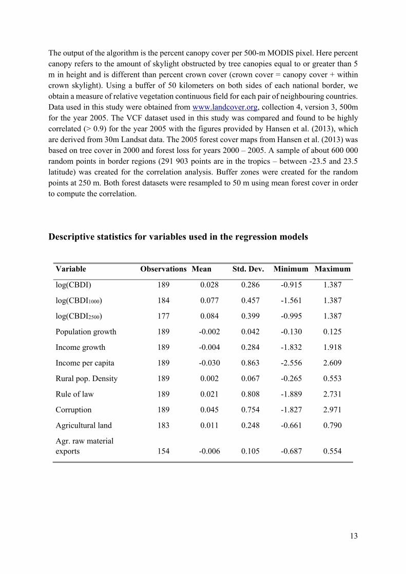
Descriptive statistics for variables used in the regression models

Variable Observations Mean Std. Dev. Minimum Maximum

log(CBDI) 189 0.028 0.286 -0.915 1.387

log(CBDI1000) 184 0.077 0.457 -1.561 1.387

log(CBDI2500) 177 0.084 0.399 -0.995 1.387

Population growth 189 -0.002 0.042 -0.130 0.125

Income growth 189 -0.004 0.284 -1.832 1.918

Income per capita 189 -0.030 0.863 -2.556 2.609

Rural pop. Density 189 0.002 0.067 -0.265 0.553

Rule of law 189 0.021 0.808 -1.889 2.731

Corruption 189 0.045 0.754 -1.827 2.971

Agricultural land 183 0.011 0.248 -0.661 0.790

Agr. raw material exports 154 -0.006 0.105 -0.687 0.554