Economic Decision-making in Poverty Depletes Behavioral Control by
41
Economic Decision-making in Poverty Depletes Behavioral Control by Dean Spears, Princeton University CEPS Working Paper No. 213 December 2010
Transcript of Economic Decision-making in Poverty Depletes Behavioral Control by

Economic Decision-making in Poverty
Depletes Behavioral Control
by
Dean Spears, Princeton University
CEPS Working Paper No. 213 December 2010
Economic decision-making in povertydepletes behavioral control
Dean Spears∗
December 9, 2010
Abstract
Economic theory and common sense suggest that time preference can cause or per-petuate poverty. Might poverty also or instead cause impatient or impulsive behavior?This paper reports a randomized lab experiment and a partially randomized field ex-periment, both in India, and analysis of the American Time Use Survey. In all threestudies, poverty is associated with diminished behavioral control. The primary contri-bution is to isolate the direction of causality from poverty to behavior; three theoreticalmechanisms from psychology cannot be definitively separated. One supported expla-nation is that poverty, by making economic decision-making more difficult for the poor,depletes cognitive control.
∗[email protected]. Princeton University. Thank you, first, to the participants, and to Vijay andDinesh for conducting the fieldwork in Banswara. John Papp, Deepak, Pramod, and Murli helped make theexperiments happen; this would have been impossible wihtout Diane Coffey. I am thankful for commentsfrom Anne Case, Angus Deaton, Josephine Duh, Mike Geruso, Simone Schaner, and Abby Sussman. Iappreciate that Sendhil Mullainathan, Eldar Shafir, and Jiaying Zhao have offered helpful suggestions anddiscussed with me their complementary studies.
1

1 Introduction
Irving Fisher (1930), detailing his Theory of Interest, explains that “a small income, other
things being equal, tends to produce a high rate of impatience.” This is both “rational” —
immediate survival is necessary to enjoy any future income or utility at all — and “irrational”
— “the effect of poverty is often to relax foresight and self-control and to tempt us to ‘trust
to luck’ for the future.”
Subsequent economists, however, have seen time preferences as causally prior properties
of persons, and important determinants of who accumulates wealth and who remains poor.
Deaton (1990) observes that allowing heterogeneity in discount rates in a theory of consump-
tion under borrowing constraints “divides the population into two groups, one of which lives
a little better than hand to mouth but never has more than enough to meet emergencies,
while the other, as a group, saves and steadily accumulates assents.” For consumers whose
impatience exceeds the rate of return to investing, remaining poor is optimal. Similarly,
Lawrance (1991) proposes different rates of time preference as “one possible explanation for
observed heterogeneity in savings behavior across socioeconomic classes,” estimating that
the poor are less patient from the fact that their consumption grows less quickly.
While time preference influences wealth directly through savings, it could also have indi-
rect effects by shaping investments in education (cf Card, 1995) or health (eg Fuchs, 1982).
The behavioral economics of time-inconsistency has further focused on implications of het-
erogeneity in discounting, present bias, and sophistication (O’Donoghue and Rabin, 1999).
Thus, Ashraf et al. (2006) argue that, absent certain institutions, hyperbolic discounters are
especially unlikely to save.
Yet, recent findings and theories in both psychology and economics suggest revisiting
Fisher’s suggestion. Indeed, poor people — like rich people — do often act impatiently.
But, if there is an association between poverty and low behavioral control, could it partially
reflect a causal effect of being poor on behavior, rather than the other way around? If so,
2

what might be the mechanism?
After reviewing three theoretical mechanisms proposed or inspired by the cognitive or
social psychological literature, this paper will report three empirical studies. Primarily,
these studies collectively identify a causal effect of poverty on behavior. Organized around
this objective, the studies cannot definitively separate the three potential mechanisms. The
best-supported explanation may be that, in these three cases, poverty appears to have made
economic decision-making more consuming of cognitive control for poorer people than for
richer people. Poverty causes difficult decisions, which deplete behavioral control.
Section 2 presents a randomized lab experiment in the field. By experimentally assigning
participants to “wealth” and “poverty” in the lab, and manipulating whether participants
made economic decisions, it identifies a causal effect of making economic decisions with
small budgets. Section 3 reports a partially randomized field experiment. Participants,
whose wealth was observed, made a real purchasing decision either before or after a task
that measured their control. Choosing first was depleting only for the poorer participants,
and this interactive effect was greatest for participants with the least cognitive resources.
Section 4 describes patterns of secondary eating in the American Time Use Survey. Unlike
other types of activity, shopping is associated with more secondary eating for poorer people,
but not for richer.
1.1 Poverty and behavior
This paper is far from the first to suggest that poverty interacts perniciously with psycho-
logical limits and biases that are common to rich and poor people. Lewis (1959), studying
Mexican slum dwellers, famously argued that poor people develop a “culture of poverty”: a
set of values that is adaptive to their poverty, but ultimately limiting.1 Banerjee (2000) de-
tailed theoretically that poverty might change behavior either by making the poor desperate,
1Other authors, outside of economics, suggesting that poverty could deter people from pursuing their owninterests or escaping poverty include Orwell (1937), Scott (1977), and Karelis (2007).
3

or by leaving them vulnerable. Bertrand et al. (2004), Duflo (2006), and Hall (2008) all have
proposed interactions between poverty and “behavioral” decision-making. Mullainathan and
Shafir (2010), whose recent studies are most complementary to those in this paper, demon-
strate greater depleting effects on math performance by New Jersey mall shoppers of an
expensive hypothetical car repair decision than an inexpensive one, with the greatest effects
on less wealthy shoppers.
Poverty may have many effects on behavior, many of which could be unrelated to be-
havioral control.2 What this paper adds to this literature is, primarily, an experimental
demonstration of a causal effect of poverty on behavioral control, induced by actual eco-
nomic decision-making in the lab and in the field. I use “behavioral control” to include
what psychologists and others write about as “willpower,” “self-control,” “self-regulation,”
or “executive” control or function: the pursuit of intentional behavioral goals, potentially
despite automatic alternative behaviors or impulses.
Three theorized mechanisms from the psychological literature could be individually or
jointly responsible for this effect of poverty. The three theoretical mechanisms are similar and
complementary. Each proposes a limited mental resource that poverty occupies or consumes,
leaving less capacity to guide or regulate behavior.
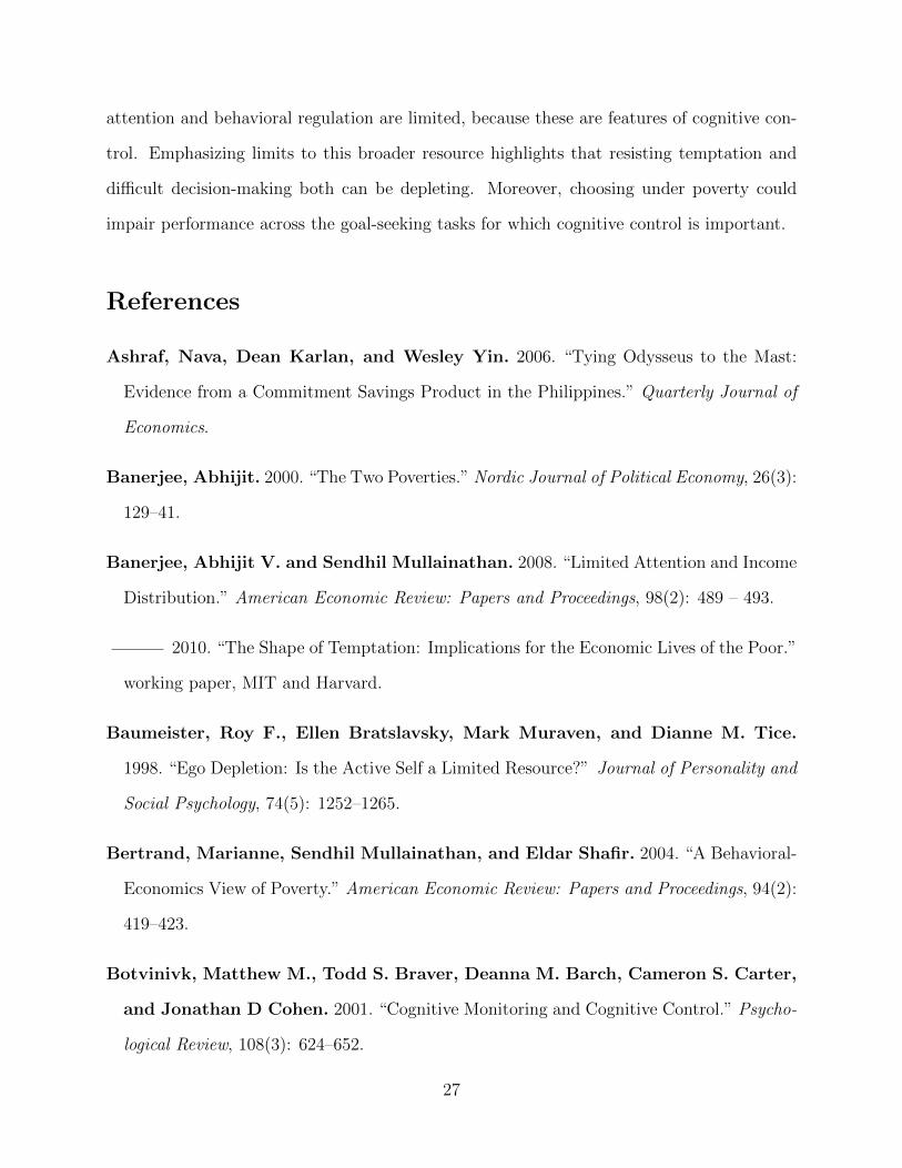
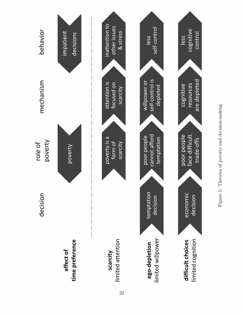
Figure 1 summaries the theories, which are detailed in the Appendix. The first mecha-
nism, highlighting scarcity, proposes that attention is limited, and is directed to whatever
domain is scarce. When poverty is the key form of scarcity facing a person, it can over-occupy
her attention, resulting in worse performance.
The other two theories propose, more narrowly, that poverty is depleting because it
changes the consequences of decision-making. The theory of ego depletion proposes that
willpower is limited, and is consumed by resisting temptation or inhibiting behavior. Applied
2In economics, for example, Case (2001) finds effects of the South African pension on stress; Ray (2006)considers poverty’s interactions with aspirations; Banerjee and Mullainathan (2010) propose that the sophis-ticatedly tempted poor will not save money that they know will be wasted in the future; Spears (2010b)finds large impacts of deliberation costs on the rural Indian poor.
4

to poverty by Ozdenoren et al. (forthcoming), this theory predicts that because poor people
cannot afford to indulge, decisions require them to resist temptation, and therefore deplete
their willpower.
Finally, the third theory suggests that it is cognitive control — the cognitive process,
associated with working memory, that directs attention and inhibits automatic behaviors to
pursue executive goals — that is the key limiting constraint. Because, in poverty, the same
economic decision represents a more conflicting trade-off among more important priorities,
economic decision-making is more difficult. These difficult decisions deplete cognitive control.
For example, Wang et al. (2010) find that, relative to participants making easier decisions,
participants making more difficult decisions involving conflicting trade-offs are more likely
to subsequently choose unhealthy snacks and entertaining, rather than educational, movies.
The three studies below strike different balances among internal and external validity.
Primarily, they separate a causal effect of poverty from the countervailing effects of time
preference. Additionally, although not definitively, they collectively may distinguish among
the theories in figure 1. Does poverty change behavior? If so, does it do so even when poor
people do not have to make decisions? If poverty’s effect depends on decision-making, is there
only an impact when the decision-maker resists temptation or uses willpower, or is there an
effect any time poverty has made an economic decision difficult? Does the effect depend
on cognitive resources? Answering these questions may help indicate which mechanism or
mechanisms may be at work in the cases studied here, but the focus will be on the direction
of causality.
2 Lab experiment in the field
In July 2010, with the assistance of two research assistants, I conducted a lab experiment
in Banswara, a small city in rural southern Rajasthan, in India. The experiment randomly
assigned “wealth” and “poverty” in the experiment’s context. This isolated an effect of
5

poverty, ruling out reverse causality or other confounds.
2.1 Procedure
The experiment had three stages. First, participants played a “store game” that required
some of them to make an economic decision. Second, participants’ behavioral control was
measured on two tasks. The experiment is designed to estimate the effect of different versions
of the store game on performance in the behavioral tasks. Third, participants were asked a
set of economic and demographic survey questions. The experiment was conducted in Vagri,
a language similar to Hindi. The research assistants did not know my hypotheses.
2.1.1 Store game: depletion
In the store game, participants were told to imagine that they are in a store with three
items: a 500ml bottle of cooking oil, a tiffin (a metal food storage container), and a bundle
of synthetic rope. Participants were randomly assigned to receive either one or two of these
items — thus, to be relatively “poor” or “rich,” although these terms were not used in the
experiment. They were independently randomly assigned to either be allowed and required
to choose which item or items they would receive, or to simply be told. Thus, each was
randomly assigned to one of four conditions:
{(rich, choice), (poor, choice), (rich, no choice), (poor, no choice)}.
In the no-choice condition, goods were given in the same distribution as they were chosen
by participants in the choice condition. In both conditions, it was made clear to participants
that they did not have to pay for the items, either out of pocket or out of their participation
payment. Randomization into receiving one or two items was done manually: the participant
pulled a card with one or two dots out of a bucket. This was done to ensure that the unequal
distribution of prizes would seem fair, but happened before the participant was told what
6

the randomization would determine to prevent anticipatory utility. Assignment to choice
conditions was done randomly in advance with a computer, and participants were not told
that having choice was a randomized experimental condition.
While not crucial to the experiment’s primary purpose of isolating a causal effect of
poverty, the oil and tiffin were used in the experiment because their interpretation might
clarify the mechanism of poverty’s effect. In this population, the cooking oil likely represented
temptation: it had a slightly lower market price, but could be eaten to add good-tasting
calories to food today. The tiffin, which offered no immediate benefit, would be an invest-
ment good, especially since almost all of the participants traveled to Banswara for work from
a home village. The rope, while valuable and chosen by a few participants, had no special
interpretation. If participants had the hypothesized preferences, “rich” participants could
afford what they wanted and did not face a difficult economic trade-off, while “poor” partici-
pants had to choose between temptation and investment. Moreover, participants who choose
the oil may be interpretable as not having used willpower to resist temptation (although they
may have attempted and failed to resist).
2.1.2 Handgrip and Stroop task: behavioral control
After playing the store game, participants’ performance was measured on two tasks: first
squeezing a handgrip and then a Stroop-like task, which will be described below. The
handgrip was commercially-purchased exercise equipment, consisting of two padded bars
connected with a spring (see figure 2). Participants were asked to squeeze the handgrip as
long as they could, and were stopped after three minutes if still squeezing. Squeezing time
ranged from a minimum of 22 seconds to a maximum of 180, with a mean of 103. Prior
research has often used handgrips to measure control.3 For example, Muraven et al. (1998)
3According to Muraven et al. (1998) “squeezing a handgrip is a well-established measure of self-regulatoryability,” because “prior research has concluded that maintaining a grip is almost entirely a measure of self-control and has very little to do with overall bodily strength” (777). Even if this is false, participants arerandomly assigned to treatments.
7

find that after being asked to control their emotions during an upsetting movie, participants
did not squeeze a similar handgrip as long as control-group participants did who merely
watched the movie.
In the Stroop-like task, participants were shown cards on which a single-digit number
was repeated several times. They were asked to say then number of times the number was
shown, not the number itself. For example, if the card shows “5 5,” the answer is “two”
not “five.” A research assistant first discussed two example cards with each participant and
then flipped one at a time through eight cards in a fixed order. Participants’ accuracy was
recorded; scores ranged from 0 to 8 with a median of 6.
The canonical Stroop (1935) task involves naming the color of the ink that a word is
printed in, not the color that the word names. This is difficult because it requires overriding
the response of reading the color word, which is more automatic. For example, Richeson and
Shelton (2003) show that experimental participants who have practiced self-regulation in an
interracial interaction perform worse in a subsequent color-naming Stroop task. They find
that performance is worsened only for those participants for whom the initial task would be
depleting: in their experiment, people with high racial prejudice scores.
In this population of Vagri-speaking day laborers, reading words would not be automatic,
as intended in the Stroop task, because many are illiterate. Flowers et al. (1979) modified
the Stroop test to use numbers. Reading numbers is more automatic than counting even
for illiterate people, due to their familiarity with money, so this Stroop-like task measures
behavioral control. For example, Mullainathan and Shafir (2010) measure the difference in
Tamil sugar cane farmers’ performance on a numerical Stroop task before and after their
harvest.
2.1.3 Participants
The experiment’s 57 participants were adult men who were recruited in the early morning
from an outdoor meeting-point that serves as an informal market for casual day labor.
8

Participants were hired to participate in the study as their work for the day and were paid
100 rupees, in addition to tea and snacks and the items they received in the experimental
game. Participants waited in a large room with a monitor until called individually and in a
random order to a smaller room for the experiment. Each participant was required to leave
the study site after the experiment.
The experiment was conducted over two consecutive days. On the second day, partici-
pants were recruited from a meeting point and a bus stand located in a different part of the
city from the first day’s recruitment site. Each participant had his picture taken at the end
of the experiment to ensure that he did not participate again the next day. No participant,
during debriefing, reported having heard of this study before coming to the experiment. The
research assistants and I believe that no participant had any information about the particular
games, decisions, and tasks in the experiment.
2.2 Econometric strategy and validity
Does economic decision-making deplete cognitive resources of the poor and worsen subse-
quent behavioral control? The answer requires an estimate of the interaction between poverty
and choice:
zi = β0 + β1poori + β2choicei + β3poori × choicei + εi, (1)
where poor and choice are dummy indicators for experimental assignment and zi is the mean
of the z-score of participant i’s performance in the two measures, squeezing time and Stroop
accuracy.
Does poverty change behavior? The causal interpretation of the coefficients derives from
the random assignment of experimental treatments. In particular, participants’ budgets were
randomly assigned, ruling out that choices determined their wealth at the lab store. Table
1 reports summary statistics for survey questions and verifies that, in this finite sample,
randomization did not produce any statistically observable differences.
9

If economic decisions in poverty deplete resources used for behavioral control, then β3
should be negative. On the other hand, if scarcity itself drives any effect of poverty on
depletion, the negative effect should be found in β2 < 0, not β3: no choice is necessary for
poverty to worsen performance through this mechanism. Alternatively, β2 can be interpreted
as controlling for experimenter demand, if participants who receive more are more willing to
perform experimental tasks.
2.3 Results
Table 2 presents the results. Being randomly assigned to face a difficult economic decision
with a small budget caused worse performance: β3 < 0. The table presents robust standard
errors, but with such a small sample, nonparametric randomization inference can be used,
randomly re-assigning outcomes to experimental groups. This procedure produces one- and
two-sided p-values of 0.023 and 0.047 for the estimate of the coefficient on the interaction.4
Columns 2 and 4 include controls for age, whether married, ever school, and whether
the participant correctly reported the day of the week. These controls are unnecessary in
a randomized experiment and potentially biasing in a finite sample (Freedman, 2008), but
are included as a robustness check. The lack of a direct effect of being assigned to receive
two goods rather than one is evidence that the performance depletion is not due to an
experimenter demand effect or reciprocity in which participants are more eager to please the
experimenter after receiving a greater gift.
Through what mechanism might experimental poverty have had this effect? There was
no direct effect of prizes being scarce but out of the participant’s control: β1 cannot be
distinguished from zero. Scarcity caused worse performance only when tests followed an
economic decision.
To be depleting, must the decision use willpower? If control were depleted only through
4Results using only handgrip or Stroop performance, rather than their mean, are similar, but not statis-tically significant in this small sample
10

the use of willpower, and if the cooking oil were a tempting good, then there would be no
interaction when restricting the sample to participants who chose or were assigned the oil if
none of these participants used willpower to resist temptation. However, as columns 3 and
4 demonstrate, if anything the effect was larger for this group, although the effect is not
statistically significantly different from the effect for the entire sample. While this suggests
that limited cognitive control, not limited willpower specifically, was the mechanism, it
cannot be ruled out that some participants who chose the oil may have first used willpower
trying to resist temptation and then succumbed, or that multiple mechanisms were active.
3 Field experiment
In July and August 2010, the same two research assistants conducted a field experiment in
rural villages of Banswara district, in Rajasthan, India. Participants made real spending
decisions. Each day both surveyors traveled to two villages, one richer and one poorer. The
surveyors offered participants a product for sale either before or after asking them to squeeze a
handgrip and recorded economic and demographic information about participants. Decision-
making proved depleting only for poorer participants. This interactive effect is greatest for
participants with the least cognitive resources.
3.1 Procedure
The experiment was conducted in a 15-minute one-on-one interview in Vagri, during an
unscheduled visit to the participant’s home. The experiment had three components: an
economic decision, squeezing a handgrip, and a set of survey questions that included a
measure of cognitive resources (the Stroop task was not used). The order of the decision
and the performance task was randomized. Half of each surveyor’s participants in each
village made the decision first, before squeezing the handgrip, and the other half squeezed
the handgrip first, before learning about the decision.
11

In the economic decision, surveyors offered participants the opportunity to purchase a
package of two 120 gram bars of handwashing and body soap for 10 rupees. The brand,
Lifebuoy, is a brand marketed for health and the price was a 60 percent discount off of
the retail price, so participants may have been tempted to take advantage of the special
offer. Surveyors explained that they received the soap from a college for this project. They
emphasized that participants could buy the soap if they wanted to, or not; that the decision
was the participant’s; and that the participant could take as long as necessary to decide.
Most only deliberated for a few seconds. Forty-three percent of participants bought the
soap, suggesting the soap was priced such that neither buying nor rejecting was an obvious
response.
The handgrip task was the same as in the lab experiment. Participants were asked to
squeeze a handgrip as long as they could, and were stopped after three minutes. Because
half of the participants squeezed the handgrip before they were aware of the soap offer, the
data can be used to estimate any direct effect of wealth on handgrip ability.
After demographic and economic survey questions, participants were given a working
memory test. The surveyor read the participant a list of five simple words, asked a set of
irrelevant survey questions, and then asked the participant to repeat as many of the words as
he could remember. The mean participant remembered less than two words. Spears (2010a)
found that a similar test predicted consumption behavior among South African pension
recipients.
The two surveyors, both male, conducted 216 valid interviews with adult males from
age 18 to 65. Interviews were conducted with the participant alone, and the surveyors were
trained to discontinue the experiment if it could not be done alone, in order to promote
anonymity and isolate individual decision-making, not social preferences. No more than one
participant was interviewed from any household. Surveyors were instructed not to interview
anybody who they suspected may have seen, overheard, or heard about the experiment be-
fore. Randomization of the order of experimental tasks was done by preparing two otherwise
12

identical versions of the survey form which were arranged into packets for each surveyor, for
each village. Therefore, random assignment was stratified within village-surveyor combina-
tions. Forms were sealed in opaque envelopes and surveyors were instructed never to look
at the next form until a participant had consented to the interview.
3.2 Econometric strategy and validity
Does economic decision-making deplete performance for the poor but not for the rich? Again,
the econometric question is whether the effect of poverty interacts with having made an
economic choice:
squeezei = β0 + β1soap firstij + β2poorij + β3soap firstij × poorij + αj +Xijθ + εij, (2)
where squeeze is time squeezed in seconds, soap first is an indicator for making the economic
decision before squeezing the handgrip, and poor represents one of the measures of poverty
that will be used. Village fixed effects αj and demographic and economic controls Xij will
be used in some specifications. Participants are indexed i and villages j. As before, I
hypothesize that the interaction β3 is negative. Three indicators of poverty will be used:
being in the bottom half of the distribution of the asset count in this sample, the surveyor’s
assessment (before economic survey questions) of whether the participant’s clothes are either
clean or torn, and the first principal component of all socioeconomic questions (ownership
of each asset as a dummy, clothes, native and mother’s village).
Soap first is randomly assigned, so it is unlikely to be correlated with many other mea-
sures. Table 3 reports summary statistics by experimental group and finds no statistically
or economically significant imbalance.
Wealth and poverty are not, of course, randomly assigned, and may be endogenously
related to handgrip squeezing. Results will be shown with and without controls for age, age2,
household size, whether married, ever school, the measure of short term memory, an indicator
13

for already having soap in the house, an indicator for somebody in the household being sick
in the past week, and fixed effects. The causal interpretation depends on the assumption
that the interaction between poverty and assignment to decide first is independent of residual
correlates of handgrip squeezing, conditional on these covariates.
The surveyors were instructed to travel to two villages together each day, one richer and
one poorer, according to a schedule set in advance. The schedule was made by selecting
the richest and poorest nearby villages, according to Indian census data. The assignment of
richer and poorer villages to the morning or afternoon was randomly counterbalanced across
days. This process ensured economic diversity in the sample and prevented wealth from
being correlated with time of the interview.
If poverty influences performance by depleting cognitive resources in particular then
the interactive effect should be least for participants with the most cognitive ability: their
resources would be less likely to become consumed. This will be tested by estimating the
full triple interaction of poverty and decision-making with the score on the working memory
test. Working memory is closely related to cognitive control (Shamosh et al., 2008) and may
be the resource used to maintain executive goals. Experimentally occupying participants’
working memory results in more impulsive behavior (Getz et al., 2009), such as choosing
chocolate cake over fruit salad (Shiv and Fedorikhin, 1999).
I hypothesize that the coefficient on the triple interaction should be positive: the neg-
ative effect of decision-making on performance for poor participants should be absent (less
negative) for those with more cognitive abilities. While the working memory test came at
the end of the experiment (to avoid influencing the main result) and may have been influ-
enced by it, by the time participants took the working memory test they had completed both
the handgrip task and the economic decision, so there would be no mechanical correlation
between their interaction and the working memory score.
14

3.3 Results
Table 4 presents the main result of the field experiment. Before being offered soap, poorer
and richer participants squeeze, on average, the same length of time. Deciding whether or
not to buy the soap had no effect on handgrip behavior for richer participants, but caused
poorer participants to squeeze for an average of 40 seconds less time, out of a mean of 108
seconds. Nonparametric randomization inference that re-randomized within surveyor-cluster
combinations found a p-value of 0.001 for the first column of panel 1.
Various indicators of poverty find the same result. This result is robust to omitting
participants who do not squeeze the handgrip at all (panel B) or to using Tobit estimates
(panel C; squeezing time could not be below zero or above 180 seconds) and to including
covariates. Indicating poverty with a different cutpoint in the asset count (the bottom third
of participants, rather than the median) produces similar results (β3 = −34s; t = −2.31).
3.3.1 Depletability causing poverty?
In the lab experiment, a causal effect of “poverty” was demonstrated with random assign-
ment. The relationship between depletion, depletability, and real-world poverty could be
complex. Even if the poor do not have lower levels of, for example, willpower than the rich,
might they have become poor or failed to escape poverty because their equal-sized stocks of
regulatory resources are more readily depleted?
In the field experiment, poverty was not randomly assigned. But depletability causing
poverty is plausible only for participants who have experienced economic mobility. Finding
the same result in a subsample restricted to participants unlikely to have been sorted into
poverty due to their depetability makes this reverse causality less plausible. One imperfect
way to isolate the effect of poverty may be to focus on participants who match the a priori
designation of their village as rich or poor from census data; another is to focus on those who
still live in the village where their mothers lived when they were born, in a society where
geographic and economic mobility are related.
15

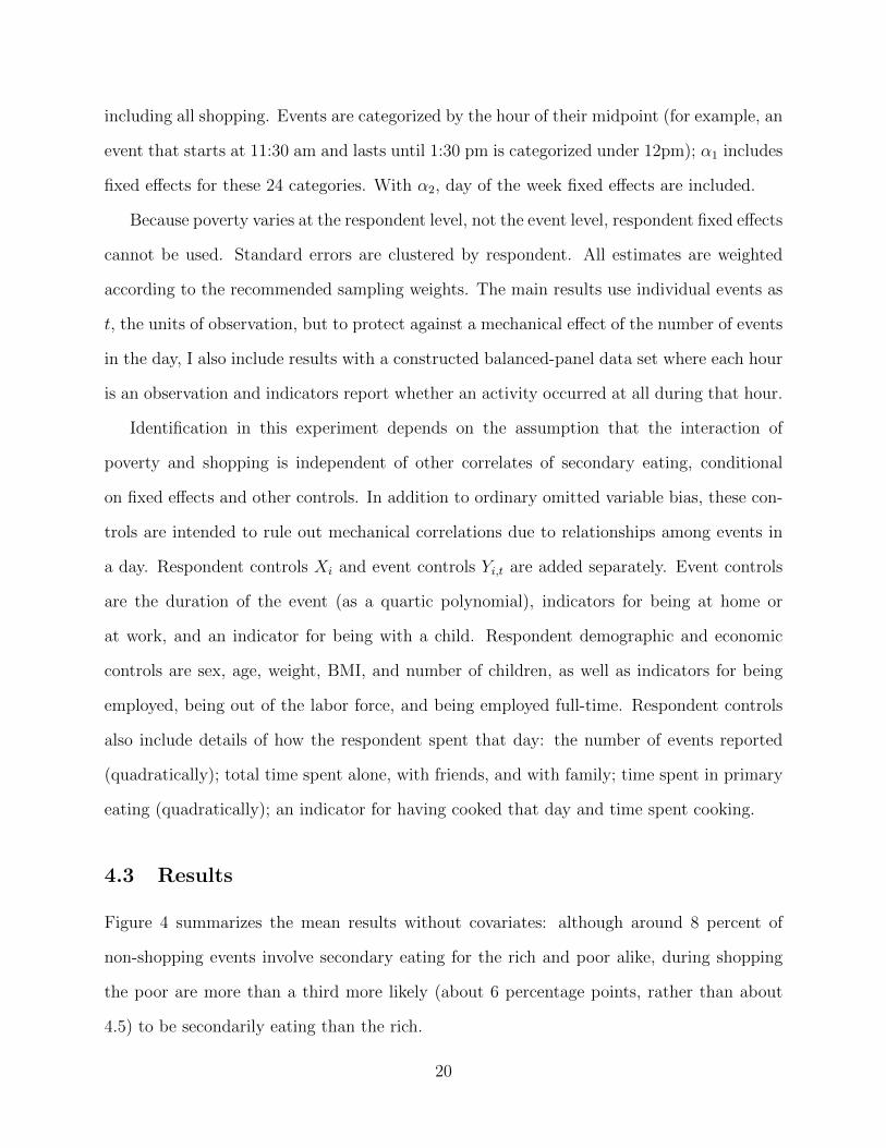
Figure 3 presents results for those participants who report still living in their native
village. Again, in both of these low-mobility sub-samples, decision-making had no effect
on the rich, but reduced squeezing time for the poor (match census: n = 131, β3 = −45s,
t = −2.66; mother lived in same village when participant born: n = 95, β3 = −60s,
t = −2.76). This suggests that it is not the case that these results are explained by those
who are most easily depleted by economic decisions being more likely to become poor.
3.3.2 Theories of poverty
Having demonstrated an effect of poverty, a secondary question is whether these data are
more consistent with some of the three mechanisms than others.
The clearest evidence for a role for cognitive resources in in the triple interaction with
working memory, reported in table 5. The key coefficient is the triple interaction, which
shows the increase in β3 in equation 2 associated with each additional word remembered
on the working memory test. Interpreting these results require summing the coefficients:
for example, in the first specification, requiring a poor participant to make the economic
decision would decrease squeezing time by an average of 54 seconds if he remembered no
words on the test, but only by an average of 40 seconds if he remembered one word, with a
similarly declining effect as the working memory score increases.
Economic decision-making worsened subsequent performance for the poor, but to a
greater degree for those with lower cognitive resources than those with higher cognitive
resources. As the table shows, this effect is robust to respecifications and nonparametric
randomization inference finds one- and two-sided p values of 0.016 and 0.050 for the triple
interaction.
As in the lab experiment, there was no direct effect of scarcity on performance. The
coefficient on poverty is statistically significant in only one of 18 regressions, where it is
positive. The effect was concentrated among those who made a decision.
Also like in the lab experiment, splitting the sample into the 86 participants who did and
16

109 participants who did not buy the soap could test whether the effect was concentrated
on those who resisted temptation, if the discounted, name-brand soap can be interpreted
as a tempting offer. Again, it was not: if anything, the interactive effect was about ten
seconds greater in absolute value for participants who bought the soap, although this triple
interaction is not significant (t = −0.50). Here, the effect was an effect of decision-making,
with no evidence of an effect of scarcity overall or resisting temptation specifically.
4 Secondary eating while shopping
The first two studies show effects of poverty on behavioral control, but not as exhibited in a
behavior with important implications: do handgrips and Stroop games matter? Moreover,
the experimental studies demonstrate depletion resulting from a particular decision: perhaps
other decisions are difficult and depleting for the rich? The third study addresses both of
these concerns by studying a cross-section of Americans making whatever spending decisions
they do at their level of wealth.
The American Time Use Survey (ATUS) provides representative data on what Americans
do during the 24 hours in a day (cf. Hamermesh et al., 2005). It records each respondent’s
primary activity at every moment of one day. In particular, it records when participants
are shopping, making economic decisions. This data is matched to household economic and
demographic data from the Current Population Survey (CPS).
In 2008, an eating and health module also recorded whether participants were secondarily
eating during each event. Secondary eating is “eating while doing other activities such
as driving or watching TV” (Bureau of Labor Statistics, 2010). Secondary eating may
sometimes reflect a failure of cognitive control: it is by definition not fully attended to,
and may not reflect the deliberate pursuit of health goals.5 “Mindless eating” without
5Hamermesh (2010), who terms secondary eating “grazing,” argues from price theory that secondaryeating will increase as earnings do (an increase in the opportunity cost of primary eating) and finds someevidence for this in the ATUS.
17

“consumption monitoring” facilitates overeating (Wansink and Sobal, 2007). For example,
in an experiment conducted by Wansink et al. (2005), treatment group participants were
unable to visually monitor their consumption because a hidden mechanism secretly refilled
their soup bowls. These participants ate 73 percent more soup than control participants
with normal, finite soup bowls, but did not believe they had eaten more or claim to feel
more sated. In the ATUS data, a one-hour increase in daily time spent secondarily eating is
linearly associated with a 0.09-point increase in BMI (two-sided p = 0.085).
Shopping and making purchases require economic decision-making. If this decision-
making is particularly depleting for poorer people, and if secondary eating is a mindless
behavior often in conflict with Americans’ health goals, then this economic decision-making
should especially encourage secondary eating among the poor. In the ATUS, shopping is
accompanied by secondary eating among poorer people more often than among richer people.
4.1 Data
This section uses the 2008 wave of the ATUS. The ATUS is sponsored by the Bureau of
Labor Statistics and conducted by the U.S. Census Bureau. It randomly selects households
that have recently participated in the CPS, and then uniformly randomly selects an adult
participant from within the household. Therefore, time use data can be matched with
respondent data from the ATUS and household data from the CPS.
Each respondent details the previous day to an interviewer in a phone interview. Days
are recorded from 4:00 am until 4:00 am on the day of the interview. Interviewers are trained
to facilitate recall by working forwards and backwards and to record verbatim descriptions
of activities. These activities are then classified according to a three-tier taxonomy; for
example “household activities” include care for “lawn, garden, and houseplants,” which
includes maintaining “ponds, pools, and hot tubs.” The median respondents reported 19
events in their days, 14 at the 25th percentile and 25 at the 75th.
The eating and health module was sponsored by the U.S. Department of Agriculture’s
18

Economic Research Service and the National Institutes of Healths National Cancer Institute.
It asked about subjective health, health indicators such as weight, and food sources and
preparation. In particular, it asked whether the respondent was secondarily eating during
each event in the daily diaries.
Of 6,923 respondents in the sample, household economic data is available for 6,711 and
personal earnings data (including values of zero) is available for 4,134. Using the categories
pre-coded in the CPS data, 13 percent of respondents lived in households with income less
than 130 percent of the poverty line, and 23 percent lived in household with less than 185
percent; I will refer to the former group as “very poor” and the latter group as “poor.”
Eight percent of all events involved secondary eating, compared with 4.6 percent of
shopping events that are not grocery shopping. Among activities, secondary eating is most
common at work, followed by during socializing or leisure. Of all events, 3.5 percent are
shopping, and the average shopping event lasts twenty minutes. Richer people shop slightly
more often, but not statistically significantly (p = 0.36).
4.2 Econometric strategy
Relative to other event types, is shopping accompanied by secondary eating more often for
poorer participants than for richer participants? I estimate the linear probability regression
secondaryit =β0 + β1shoppingi,t × richeri + β2shoppingi,t + β3richeri+
θXi + ϑYi,t + α1hourt + α2dayt + εi,t,(3)
where i indexes respondents and t indexes events in i’s day. Secondary is an indicator of
secondary eating by i during event t; shopping indicates whether t was a shopping event for
i, and richer is either an indicator that the participant’s household is not poor in the CPS or
her weekly earnings. In most specifications, I include only non-grocery shopping in shopping
to prevent a confounding effect of food availability, but results will be shown to be robust to
19
including all shopping. Events are categorized by the hour of their midpoint (for example, an
event that starts at 11:30 am and lasts until 1:30 pm is categorized under 12pm); α1 includes
fixed effects for these 24 categories. With α2, day of the week fixed effects are included.
Because poverty varies at the respondent level, not the event level, respondent fixed effects
cannot be used. Standard errors are clustered by respondent. All estimates are weighted
according to the recommended sampling weights. The main results use individual events as
t, the units of observation, but to protect against a mechanical effect of the number of events
in the day, I also include results with a constructed balanced-panel data set where each hour
is an observation and indicators report whether an activity occurred at all during that hour.
Identification in this experiment depends on the assumption that the interaction of
poverty and shopping is independent of other correlates of secondary eating, conditional
on fixed effects and other controls. In addition to ordinary omitted variable bias, these con-
trols are intended to rule out mechanical correlations due to relationships among events in
a day. Respondent controls Xi and event controls Yi,t are added separately. Event controls
are the duration of the event (as a quartic polynomial), indicators for being at home or
at work, and an indicator for being with a child. Respondent demographic and economic
controls are sex, age, weight, BMI, and number of children, as well as indicators for being
employed, being out of the labor force, and being employed full-time. Respondent controls
also include details of how the respondent spent that day: the number of events reported
(quadratically); total time spent alone, with friends, and with family; time spent in primary
eating (quadratically); an indicator for having cooked that day and time spent cooking.
4.3 Results
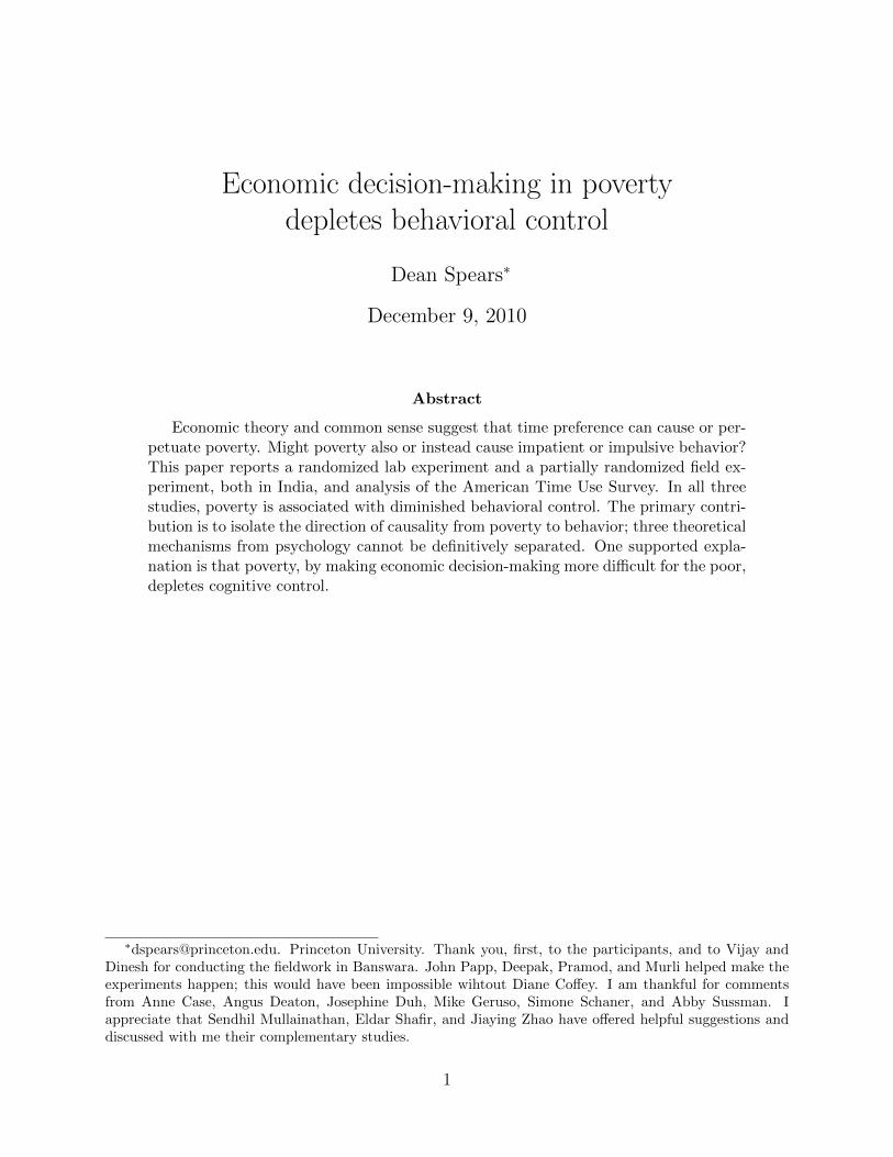
Figure 4 summarizes the mean results without covariates: although around 8 percent of
non-shopping events involve secondary eating for the rich and poor alike, during shopping
the poor are more than a third more likely (about 6 percentage points, rather than about
4.5) to be secondarily eating than the rich.
20

Table 6 confirms that this interaction is similar and statistically significant even after
including a range of controls. The estimate that the association between shopping and
secondary eating is about two percentage points greater for poor people is robust to various
respecifications.6
Beginning in column three, a similar interaction between poverty and housework is in-
cluded as a placebo. It is not statistically distinguishable from zero and does not change the
estimates for shopping. Additionally, measuring economic well-being with personal earnings
produces a similar interaction: for participants with mean earnings, shopping is associated
with a 1.2 percentage point increase in secondary eating, an association that becomes nega-
tive for participants with weekly earnings more than $81 above the mean.
The right-side panel excludes events when the respondent is sleeping or primarily eating,
as these cannot involve secondary eating, so they cannot show a difference across the rich and
poor. Effects are similar, even greater in magnitude for the main specification. Including
grocery shopping among shopping or restricting the indicator of poverty to the poorest
produces comparable estimates.
Table 7 reports a set of placebo regressions. The final specification from column 5 of
table 6 is repeated with events during which the theory does not predict an interactive ef-
fect: leisure time, watching tv, doing housework, being at work, and the lag of the shopping
variable. None of these event types statistically significantly reproduces the negative inter-
action with shopping. The positive coefficient on work may reflect different types of jobs, or
a spurious result of running many regressions.
Table 8 estimates the same specification with hours, rather than events, as the units of
observation. For each hour in each respondent’s day, I constructed indicators of whether
the respondent went shopping during any part of that hour and whether the respondent
did any secondary eating during that hour, as well as similar indicators for the covariates.
6While not reported in the table, estimating the logit of secondary eating in equation 3 produces a similarmarginal effect of 2.8 percentage points for β1, with a two-sided p-value of 0.062.
21

Richer respondents are more likely than poorer respondents to be secondarily eating while
not shopping, but less likely while shopping.
As a final robustness check, the right-hand panel includes results for secondary drinking.
Secondary drinking is more difficult to interpret because it includes both, for example, soft
drink consumption — which may be inconsistent with health goals — and coffee consump-
tion, which may promote goals and occurs often and continuously during events of long
duration. Secondary drinking accompanies 16 percent of events. Nevertheless, a negative
coefficient may be expected if secondary drinking is done mindlessly or impulsively. The
results show that during shopping the frequency of secondary drinking increases for poorer
people, but does not change or slightly decreases for richer people.
4.4 Interpretation
These results are consistent with the prediction that economic decision-making will cause
depleted behavioral control specifically among the poor, but it cannot be ruled out that they
are driven by an omitted correlation. For example, poor people may go to different stores,
shop differently, or have different health goals.
Unlike in the field experiment, no measure of working memory is available to isolate a
specifically cognitive mechanism. However, in general and as before, poor people are not
unconditionally more likely to be secondarily eating, suggesting that any effect is not caused
by scarcity alone. Moreover, there is no direct evidence that respondents were resisting
temptation while shopping, only that they were making purchasing choices. These findings
are consistent with the theory of limited cognitive control, but a combination of the three
cannot be ruled out.
22

5 Conclusions and discussion
Economic decision-making had negative effects on controlled behavior when participants
were poorer. This may be because for poorer participants, decisions required more difficult
trade-offs, and were more depleting of cognitive resources.
Random assignment of experimental “poverty” in the lab experiment and regression-
controlled and subsample analysis in the field experiment and survey data underscore that, in
these data, poverty causes depleted performance, rather than the other way around. Results
show little specific support for theories of a particular role for depletable willpower or a
generic effect of scarcity. In the field experiment, heterogeneous effects according to working
memory are consistent with a theory of poverty’s effect on cognitive control. However, all
three of these mechanisms could be active and important, especially in other populations or
contexts.
Certainly rich people, too, sometimes face difficult economic decisions; these may some-
times be depleting. However, the decisions studied in the experiments had behavioral effects
even at tiny financial magnitudes, small enough that the poor must face them routinely.
Moreover, the time-use data found that shopping’s depleting effect was limited to the poor
when rich and poor respondents made whatever purchases they made in a representative
day. Although a richer person’s budget may enable her to face a difficult choice between,
perhaps, two vacations, she also has the option of not making this choice at all. If, as the lab
experiment suggests, even routine food decisions are costly and difficult for the very poor,
then their depleting effect is more inescapable.
These studies add to the growing evidence for a cognitive dimension of what is typically
considered time preference. Additionally, they could be important for policy. Gilens (1999)
summarizes his research on American political attitudes: “In large measure, Americans hate
welfare because they view it as a program that rewards the undeserving poor” — here, the
lazy, impulsive, myopic poor. This view that poverty is caused by bad decisions and bad
23

behavior is commonly held and politically influential, but may be moderated by evidence of
the potential complexity of the causal ties between poverty and behavioral control.
A Theories of poverty and behavioral control
A.1 Scarcity & limited attention
Mullainathan and Shafir (2010) propose that poverty is psychologically important because
it is a form of scarcity. Scarcity, they suggest, causes people to experience stress and to
focus their attention on the domains where resources seem most scarce. Because attention
is limited, people attend to what is scarce to the exclusion of other potentially important
decisions. Importantly, in this model poverty is merely one form of scarcity; limits to,
for example, a busy person’s time or a dieter’s meals would produce similar psychological
results.7
Mullainathan and Shafir report interviews with Indian sugar cane farmers before and
after their harvests: before, outcomes are uncertain and resources are scarce; after, some un-
certainty is resolved and resources are more plentiful if farmers were credit constrained. After
the harvest, farmers exhibit less stress and perform better on the Stroop test, which requires
participants to override an impulsive, but wrong, answer with a deliberative response.
A.2 Ego-depletion & limited willpower
“Ego-depletion” is Baumeister et al.’s (1998) name for their theory that self-control is pro-
duced with a limited willpower stock that is temporarily used up when people regulate their
emotions or resist temptation. Thus, because “exerting self-control may consume self-control
strength, reducing the amount of strength available for subsequent self-control efforts,” Mu-
7This theory is related to, but not identical to, Banerjee and Mullainathan’s (2008) model of agents whocan allocate a unit of attention to home or work. Because poor people are unable to afford security at home,they are distracted from being productive at work whether or not a problem ultimately arises at home.
24

raven and Baumeister (2000) suggest that “self-control operates like a muscle.”
While ego-depletion was not originally intended as a theory of poverty, the need for self-
control may arise particularly often for the poor. Spending money and spending willpower
can be substitutes. Many offers of tempting purchases that are easily affordable for richer
people require a poorer person to use willpower and save her money instead.8 If willpower
is limited, and if a poorer person can afford less indulgence, then poverty will deplete self-
control when the poor face expensive temptation.
Ozdenoren et al. (forthcoming) develop an economic model of the optimal response to
temptation given finite willpower. Even a poorer person with the same amount of willpower
as a richer person must resist temptation more often. Therefore their model predicts that
“behavioral differences between rich and poor people sometimes attributed to differences in
self-control skills may reflect wealth differences and nothing more.”
A.3 Difficult choices & limited cognitive control
Cognitive resources play an important role in economic behavior because they facilitate eco-
nomic deliberation and global decision-making. Burks et al. (2008) find that in addition to
choosing larger, later payments in the lab, truck drivers with better performance on cog-
nitive tests are more likely to keep their job long enough to avoid incurring a costly debt
for training. In a field experiment among pension recipients in Cape Town, consumption
declines less steeply across the pension month among participants who show more cogni-
tive ability on a working-memory test (Spears, 2010a). Lab experiments that manipulate
cognitive resources by depleting them find similar results. Together, these results suggest
that behaviors commonly attributed to attitudes such as “impatience” may actually reflect
cognitive regulation of behavior.
8For example, Banerjee and Mullainathan (2010) explore implications of agents’ sophistication about their“declining temptation” — the idea “that the fraction of the marginal dollar that is spent on temptation goodsdecreases with overall consumption,” where temptation goods are goods in a multi-period/multi-self modelthat only generate utility for the self of the period when they are consumed. They justify this assumptionpartially with the observation that temptations such as tasty foods are satiable.
25

A third mechanism by which poverty could influence subsequent decision-making is by
taxing cognitive control. Cognitive control facilitates “the ability to select a weaker, task-
relevant response. . . in the face of competition from an otherwise stronger, but task-irrelevant
one” (Miller and Cohen, 2001). Cognitive control responds to conflict in mental processing
(Botvinivk et al., 2001), is used to make decisions (McGuire and Botvinick, 2010), and may
employ working memory to direct attention, inhibit impulses, override automatic processes,
and maintain goals. Cognitive control is limited (Monsell, 2003), and may be “depletable”
in the sense that monitoring processes can be occupied (Robinson et al., 2010).
Experimental evidence confirms that difficult choices are cognitively costly. Vohs et al.
(2008) report experiments in which, after making choices, participants showed less stamina
and persistence and more procrastination than a control group that did not choose. This
is unsurprising given evidence of deliberation costs, especially costs of economic decision-
making. Tversky and Shafir (1992) find that people avoid making difficult trade-offs, de-
ferring choice when options are in conflict, such that no option dominates another. Kool
et al. (forthcoming) demonstrate that participants choose actions to avoid cognitive demand,
but that this inclination responds to incentives. In a field experiment in rural India, Spears
(2010b) finds that price sensitivity depends on the interaction between price and decision
costs. The results are consistent with a model predicting that, faced with a given offer,
poorer people will pay deliberation costs more often and be more likely to forego valuable
opportunities.
Limits to cognitive control matter to poor people because poverty raises the stakes of
many economic decisions. For poorer people, the same economic decision may represent a
more difficult trade-off between more valuable alternatives with less margin for error. Such
decisions would demand more costly deliberation — including, but not only, when emotions
must be regulated. If cognitive resources are limited, this would leave less remaining cognitive
control for other decisions or behaviors.
To propose that cognitive control is limited is to agree with the other two models that
26
attention and behavioral regulation are limited, because these are features of cognitive con-
trol. Emphasizing limits to this broader resource highlights that resisting temptation and
difficult decision-making both can be depleting. Moreover, choosing under poverty could
impair performance across the goal-seeking tasks for which cognitive control is important.
References
Ashraf, Nava, Dean Karlan, and Wesley Yin. 2006. “Tying Odysseus to the Mast:
Evidence from a Commitment Savings Product in the Philippines.” Quarterly Journal of
Economics.
Banerjee, Abhijit. 2000. “The Two Poverties.” Nordic Journal of Political Economy, 26(3):
129–41.
Banerjee, Abhijit V. and Sendhil Mullainathan. 2008. “Limited Attention and Income
Distribution.” American Economic Review: Papers and Proceedings, 98(2): 489 – 493.
2010. “The Shape of Temptation: Implications for the Economic Lives of the Poor.”
working paper, MIT and Harvard.
Baumeister, Roy F., Ellen Bratslavsky, Mark Muraven, and Dianne M. Tice.
1998. “Ego Depletion: Is the Active Self a Limited Resource?” Journal of Personality and
Social Psychology, 74(5): 1252–1265.
Bertrand, Marianne, Sendhil Mullainathan, and Eldar Shafir. 2004. “A Behavioral-
Economics View of Poverty.” American Economic Review: Papers and Proceedings, 94(2):
419–423.
Botvinivk, Matthew M., Todd S. Braver, Deanna M. Barch, Cameron S. Carter,
and Jonathan D Cohen. 2001. “Cognitive Monitoring and Cognitive Control.” Psycho-
logical Review, 108(3): 624–652.
27

Bureau of Labor Statistics. 2010. “American Time Use Survey: Eating & Health Module
Questionnaire.” online: http://www.bls.gov/tus/ehmquestionnaire.pdf.
Burks, Stephen V, Jeffrey P. Carpenter, Lorenz Gotte, and Aldo Rustichini.
2008. “Cognitive Skills Explain Economic Preferences, Strategic Behavior, and Job At-
tachment.” Discussion Paper 3609, IZA.
Card, David. 1995. “Earnings, Schooling, and Ability Revisited.” in Solomon Polachek ed.
Research in Labor Economics, 14: JAI Press.
Case, Anne. 2001. “Does Money Protect Health Status? Evidence from South African
Pensions.” working paper 8495, NBER.
Deaton, Angus. 1990. “Saving in Developing Countries: Theory and Review.” Proceedings
of the World Bank Annual Conference on Development Economics 1989: 61–96.
Duflo, Esther. 2006. “Poor but Rational?” in Roland Benabou Abhijit Vinayak Banerjee
and Dilip Mookherjee eds. Understanding Poverty: Oxford.
Fisher, Irving. 1930. The Theory of Interest: Macmillan.
Flowers, John H., Jack L. Warner, and Michael L Polansky. 1979. “Response and
encoding factors in “ignoring” irrelevant information.” Memory & Cognition, 7(2): 86–94.
Freedman, David A. 2008. “On regression adjustments to experimental data.” Advances
in Applied Mathematics, 40: 180–93.
Fuchs, Victor R. 1982. “Time preference and health: an exploratory study.” in Victor R.
Fuchs ed. Economic Aspects of Health: Chicago and NBER.
Getz, Sarah J., Damon Tomlin, Leigh E. Nystrom, Jonathan D. Cohen, and
Andrew R. A Conway. 2009. “Executive control of intertemporal choice: Effects of
28

cognitive load on impulsive decision-making.” poster presented at Psychonomics, Prince-
ton.
Gilens, Martin. 1999. Why Americans Hate Welfare, Chicago: University of Chicago.
Hall, Crystal. 2008. “Decisions under Poverty: A Behavioral Perspective on the Decision
Making of the Poor.” Ph.D. dissertation, Princeton University.
Hamermesh, Daniel S. 2010. “Incentives, time use and BMI: The roles of eating, grazing
and goods.” Economics and Human Biology, 8: 2–15.
Hamermesh, Daniel S., Harley Frazis, and Jay Stewart. 2005. “Data Watch: The
American Time Use Survey.” Journal of Economic Perspectives, 19(1): 221–232.
Karelis, Charles. 2007. The Persistence of Poverty: Yale.
Kool, Wouter, Joseph T. McGuire, Zev B. Rosen, and Matthew M Botvinick.
forthcoming. “Decision Making and the Avoidance of Cognitive Demand.” Journal of
Experimental Psychology: General.
Lawrance, Emily C. 1991. “Poverty and the Rate of Time Preference: Evidence from
Panel Data.” Journal of Political Economy, 99(1): 54–77.
Lewis, Oscar. 1959. Five Families, New York: Basic.
McGuire, Joseph T. and Matthew M Botvinick. 2010. “Prefrontal Cortex, cognitive
control, and the registration of decision costs.” PNAS, 107(17): 7922–7926.
Miller, Earl K. and Jonathan D Cohen. 2001. “An Integrative Theory of Prefrontal
Cortex Function.” Annual Review of Neuroscience, 24: 167–202.
Monsell, Stephen. 2003. “Task Switching.” TRENDS in Cognitive Sciences, 7(3): 134–140.
Mullainathan, Sendhil and Eldar Shafir. 2010. “Decisions under Scarcity.” presentation,
RSF Summer Institute for Behavioral Economics.
29

Muraven, Mark and Roy F. Baumeister. 2000. “Self-Regulation and Depletion of Lim-
ited Resources: Does Self-Control Resemble a Muscle?” Psychological Bulletin, 126(2):
247 – 259.
Muraven, Mark, Dianne M. Tice, and Roy F. Baumeister. 1998. “Self-Control as
a Limited Resource: Regulatory Depletion Patterns.” Journal of Personality and Social
Psychology.
O’Donoghue, Ted and Matthew Rabin. 1999. “Doing it Now or Later.” American
Economic Review, 89(1): 103–124.
Orwell, George. 1937. The Road to Wigan Pier: Gollancz.
Ozdenoren, Emre, Stephen Salant, and Dan Silverman. forthcoming. “Willpower and
the Optimal Control of Visceral Urges.” Journal of the European Economic Association.
Ray, Debraj. 2006. “Aspirations, Poverty and Economic Change.” in Abhijit Banerjee,
Roland Benabou, and Dilip Mookherjee eds. Understanding Poverty: Oxford.
Richeson, Jennifer A. and J. Nicole Shelton. 2003. “When Prejudice Does Not Pay:
Effects of Interracial Contact on Executive Function.” Psychological Science, 14(3): 287–
290.
Robinson, Michael D., Brandon J. Schmeichel, and Michael Inzlicht. 2010. “A
Cognitive Control Perspective of Self-Control Strength and Its Depletion.” Social and
Personality Psychology Compass, 4(3): 189200.
Scott, James. 1977. The Moral Economy of the Peasant: Rebellion and Subsistence in
Southeast Asia: Yale.
Shamosh, Noah A., Colin G. DeYoung, Adam E. Green, Diedre L. Reis,
Matthew R. Johnson, Andrew R. A. Conway, Randall W. Engle, Todd S.
30

Braver, and Jeremy R. Gray. 2008. “Individual Differences in Delay Discounting.”
Psychological Science, 19(9): 904–911.
Shiv, Baba and Alexander Fedorikhin. 1999. “Heart and Mind in Conflict: the Interplay
of Affect and Cognition in Consumer Decision Making.” Journal of Consumer Research,
26.
Spears, Dean. 2010a. “Bounded Intertemporal Rationality: Apparent Impatience among
South African Pension Recipients.” working paper, Princeton.
2010b. “Decision Costs and Price Sensitivity: Theory and Field Experimental Evi-
dence.” working paper, Princeton.
Stroop, J. Ridley. 1935. “Studies of interference in serial verbal reactions.” Journal of
Experimental Psychology, 18: 643 – 662.
Tversky, Amos and Eldar Shafir. 1992. “Choice under conflict: The dynamics of deferred
decision.” Psychological Science, 3(6): 358 – 361.
Vohs, Kathleen D., Roy F. Baumeister, Brandon J. Schmeichel, Jean M. Twenge,
Noelle M. Nelson, and Dianne M Tice. 2008. “Making Choices Impairs Subsequent
Self-Control: A Limited-Resource Account of Decision Making, Self-Regulation, and Ac-
tive Initiative.” Journal of Personality and Social Psychology, 94(5): 883 – 898.
Wang, Jing, Nathan Novemsky, Ravi Dhar, and Roy F Baumeister. 2010. “Trade-
Offs and Depletion in Choice.” Journal of Marketing Research, 47: 910 – 919, October.
Wansink, Brian and Jeffery Sobal. 2007. “Mindless Eating : The 200 Daily Food Deci-
sions We Overlook.” Environment and Behavior, 39(1): 106–123.
Wansink, Brian, James E. Painter, and Jill North. 2005. “Bottomless Bowls: Why
Visual Cues of Portion Size May Influence Intake.” Obesity Research, 13(1): 93–100.
31
pove
rty
is a
fo
rm o
f sc
arci
ty
atte
ntio
n is
fo
cuse
d on
sc
arci
ty
inat
tent
ion
to
othe
r iss
ues
& s
tres
s
tem
ptat
ion
deci
sion
poor
peo
ple
cann
ot a
ffor
d te
mpt
atio
n
will
pow
er o
r se
lf-co
ntro
l is
depl
eted
less
self-
cont
rol
econ
omic
de
cisi
on
poor
peo
ple
face
diff
icul
t tr
ade-
offs
cogn
itive
re
sour
ces
are
depl
eted
less
co
gniti
ve
cont
rol
scar
city
limite
d at
tent
ion
ego-
depl
etio
nlim
ited
will
pow
er
diff
icul
t cho
ices
limite
d co
gniti
on
deci
sion
role
of
pove
rty
mec
hani
smbe
havi
or
impa
tient
deci
sion
spo
vert
yef
fect
of
tim
e pr
efer
ence
Fig
ure
1:T
heo
ries
ofp
over
tyan
ddec
isio
n-m
akin
g
32

Figure 2: Two handgrips, similar to the ones used in the experiments
Table 1: Lab experiment: Summary statistics by experimental group
no choice choicerich poor rich poor F3,53
age 26.65 27.54 24.00 26.73 28.00 0.64married 0.95 0.92 0.92 0.93 1.00 0.40school 0.70 0.69 0.62 0.80 0.69 0.37knows day of week 0.61 0.69 0.54 0.47 0.75 1.08n 57 13 13 15 16
33

0
20
40
60
80
100
120
140
rich poor
hand
grip
squ
eezi
ng d
urat
ion
(sec
onds
)
soap decision first handgrip first n = 95; F3,31=2.95
Figure 3: Field experiment: Results for participants who live in natal villages
0
0.01
0.02
0.03
0.04
0.05
0.06
0.07
0.08
0.09
<130% of z > 185% of z
Freq
ue
ncy
of
seco
nd
ary
eati
ng
not shopping shopping
Figure 4: Time use: Secondary eating by poverty status
34

Table 2: Lab experiment: Performance z-scores by experimental treatment
(1) (2) (3) (4)full sample chose or given oil
poor 0.0627 0.0835 0.541 0.794(0.253) (0.260) (0.463) (0.362)
choice 0.532 0.565 0.519 0.577(0.213) (0.209) (0.225) (0.226)
poor × choice -0.726 -0.736 -1.402 -1.645(0.342) (0.370) (0.550) (0.451)
covariates X Xc -0.125 0.385 -0.125 0.452
(0.164) (0.348) (0.167) (0.341)n 57 57 36 36
Robust standard errors in parentheses. Covariates are age, whether married, ever school, and whether the
participant correctly reported the day of the week. The dependent variable is the mean of the respondent’s
standardized z score of handgrip and Stroop performance.
Table 3: Field experiment: Summary statistics by randomized group
x handgrip first decision first tage 38.3 38.4 38.3 0.07household size 5.72 5.64 5.81 0.58asset count 4.82 4.65 5.00 1.08soap in house 0.74 0.70 0.78 1.40member sick in last week 0.51 0.48 0.54 0.89bought soap 0.43 0.41 0.44 0.37memory test 1.54 1.41 1.67 1.44order within cluster 4.40 4.25 4.55 1.01match rich/pooor village 0.61 0.62 0.59 0.63n 216 110 106
35

Table 4: Poverty-mediated effects of economic decision-making on handgrip behavior
Panel A: Seconds squeezed handgrip, OLSlow assets clothes dirty & torn poverty index
soap first 8.317 1.386 -12.36 -16.77** -13.83** -17.04**(8.001) (8.911) (8.116) (7.357) (6.497) (6.737)
poverty 9.103 19.07 -11.15 0.374 -2.056 0.203(10.95) (11.48) (15.36) (15.87) (2.416) (3.650)
interaction -47.14*** -43.56*** -41.76* -39.98* -6.652** -6.780*(13.45) (12.09) (22.14) (22.62) (3.041) (3.495)
covariates X X Xc 111.2*** 11.13 118.1*** 17.47 118.0*** 26.33
(6.688) (47.35) (5.779) (48.68) (4.730) (42.01)n 216 211 216 211 216 211
Panel B: Seconds squeezed handgrip, conditional on squeezing, OLSlow assets clothes dirty & torn poverty index
soap first 6.388 1.556 -1.001 -5.860 -3.047 -8.281(7.564) (8.581) (7.278) (7.300) (6.168) (6.594)
poverty 6.592 10.05 -4.010 -2.130 0.331 -0.689(9.056) (10.15) (12.93) (13.92) (2.163) (2.984)
interaction -21.69* -22.44* -37.96* -39.31* -3.207 -3.426(11.87) (12.03) (18.99) (21.95) (2.928) (3.274)
covariates X X Xc 118.0*** 44.23 122.2*** 46.79 121.2*** 51.93
(5.732) (40.27) (5.553) (41.60) (4.794) (37.91)n 195 190 195 190 195 190
Panel C: Seconds squeezed handgrip, Tobitlow assets clothes dirty & torn poverty index
soap first 7.108 -0.928 -17.68* -22.96*** -19.74** -23.45***(11.17) (10.63) (9.207) (8.411) (8.177) (7.747)
poverty 11.30 23.70* -10.90 3.680 -2.256 0.628(11.75) (13.31) (17.18) (16.33) (2.908) (4.094)
interaction -57.50*** -53.56*** -52.45* -50.79* -8.249** -8.634**(17.14) (15.66) (27.11) (25.89) (3.936) (3.940)
covariates X X Xc 113.4*** 9.871 121.4*** 15.84 121.6*** 27.08
(8.435) (50.64) (6.201) (50.21) (5.547) (49.61)n 216 211 216 211 216 211
Clustered standard errors in parentheses (33 village-surveyor combinations). * p < 0.10; ** p < 0.05 ; ***
p < 0.01. Covariates are age, age2, household size, whether married, ever school, a measure of short term
memory, an indicator for already having soap in the house, an indicator for somebody in the household
being sick in the past week, and a fixed effect. In panels A and C, not squeezing is counted as zero seconds.
36

Tab
le5:
Squee
zing
inse
conds:
Inte
ract
ive
effec
tdep
ends
onco
gnit
ive
reso
urc
es
(1)
(2)
(3)
(4)
(5)
(6)
(7)
(8)
(9)
Pan
elA
:O
LS
Pan
elB
:sq
z>
0P
anel
C:
Tob
itdec
isio
nfirs
t25
.58
33.8
025
.78
8.95
012
.09
6.51
028
.51
38.1
0*27
.47
(21.
16)
(21.
74)
(22.
82)
(17.
58)
(18.
96)
(19.
95)
(19.
89)
(20.
94)
(22.
24)
poor
41.0
1**
37.6
5**
30.0
9*27
.60
22.0
215
.64
43.9
5*38
.42
27.9
5(1
7.40
)(1
8.14
)(1
7.69
)(1
8.58
)(1
6.66
)(1
6.84
)(2
2.44
)(2
4.13
)(2
4.23
)dec
isio
n×
poor
-79.
29**
*-8
7.68
***
-77.
69**
*-2
7.87
-37.
92-3
4.36
-94.
32**
*-1
03.6
***
-91.
32**
*(2
5.97
)(2
5.89
)(2
6.60
)(2
3.60
)(2
4.00
)(2
4.57
)(2
4.13
)(2
4.38
)(2
4.27
)co
gnit
ion
17.1
9***
24.3
1***
15.7
9***
10.1
315
.77*
**9.
925*
19.1
0**
27.1
7***
16.0
7**
(5.9
75)
(5.3
54)
(5.9
50)
(6.1
55)
(5.1
72)
(5.6
95)
(7.4
44)
(6.8
45)
(7.8
06)
poor×
cogn
itio
n-1
6.41
*-1
6.73
**-1
5.07
**-1
1.20
-12.
89*
-11.
40-1
4.91
-14.
41*
-12.
07(9
.059
)(7
.862
)(7
.549
)(8
.645
)(7
.480
)(7
.422
)(9
.631
)(8
.658
)(8
.587
)dec
isio
n×
cogn
itio
n-1
1.02
-16.
13*
-13.
35-3
.029
-5.7
31-4
.022
-12.
96-1
8.90
**-1
5.18
(8.3
36)
(8.3
60)
(8.7
11)
(8.1
81)
(7.6
43)
(7.9
45)
(8.4
59)
(9.0
41)
(9.5
09)
deci
sion×
poor
24.8
0**
35.2
5***
35.0
7***
6.17
917
.35†
18.4
4*26
.81*
*38
.27*
**38
.19*
**×
cogn
itio
n(1
2.33
)(1
1.62
)(1
1.44
)(1
0.79
)(1
1.08
)(1
1.11
)(1
1.61
)(1
2.49
)(1
2.08
)ag
e-1
.317
***
-0.9
24**
*-1
.693
***
(0.3
57)
(0.3
11)
(0.4
02)
clust
erF
EX
XX
XX
Xc
78.5
2***
55.8
0**
126.
8***
98.0
0***
84.3
9***
134.
3***
76.6
6***
53.5
1**
145.
7***
(14.
58)
(27.
48)
(31.
54)
(14.
51)
(26.
67)
(29.
33)
(17.
97)
(21.
42)
(33.
57)
n21
421
421
219
319
319
121
421
421
2C
lust
ered
stan
dar
der
rors
inpar
enth
eses
(33
villa
ge-s
urv
eyor
com
bin
atio
ns)
.“C
ognit
ion”
issc
ore
0-5
ona
wor
kin
gm
emor
yte
st.
“sqz>
0”is
OL
Sco
ndit
ional
onsq
uee
zing
ap
osit
ive
amou
nt
ofti
me.
Inpan
els
Aan
dC
,not
squee
zing
isco
unte
das
zero
seco
nds.
*p<
0.10
;**
p<
0.05
;**
*p<
0.01
;†p
=0.
12.
37

Tab
le6:
Sec
ondar
yea
ting:
linea
rpro
bab
ilit
yduri
ng
anev
ent
Fu
llsa
mp
leS
ub
sam
ple
ofev
ents
excl
ud
ing
slee
pin
gan
dp
rim
ary
eati
ng
(1)
(2)
(3)
(4)
(5)
(6)
(7)
(8)
shop
pin
g:n
ogr
oce
ries
no
groce
ries
no
groce
ries
no
groce
ries
no
groce
ries
inc.
gro
ceri
esn
ogro
ceri
esn
ogro
ceri
esri
cher
:n
otp
oor
not
poor
not
poor
earn
ings
not
poor
not
poor
not
v.
poor
earn
ings
shop
pin
g×
rich
er-0
.022
8**
-0.0
226*
*-0
.023
4**
-0.0
151*
-0.0
251*
*-0
.0162*
-0.0
192†
-0.0
118††
(0.0
113)
(0.0
112)
(0.0
112)
(0.0
0782
)(0
.010
8)(0
.00844)
(0.0
124)
(0.0
0775)
shop
pin
g0.
0314
***
0.03
13**
*0.
0318
***
0.01
22**
0.00
645
-0.0
0828
0.0
0340
-0.0
152***
(0.0
102)
(0.0
101)
(0.0
101)
(0.0
0550
)(0
.009
72)
(0.0
0747)
(0.0
116)
(0.0
0544)
rich
er0.
0073
7*0.
0084
8**
0.00
928*
*0.
0018
20.
0076
00.0
0747
0.0
0585
-0.0
00127
(0.0
0396
)(0
.004
22)
(0.0
0429
)(0
.004
34)
(0.0
0554
)(0
.00559)
(0.0
0676)
(0.0
0546)
hou
sew
ork×
rich
er-0
.013
8-0
.003
57-0
.006
93-0
.00686
-0.0
108
-0.0
0552
(0.0
101)
(0.0
0813
)(0
.010
4)(0
.0104)
(0.0
135)
(0.0
0803)
hou
sew
ork
0.00
448
-0.0
0816
-0.0
189*
*-0
.0191**
-0.0
148
-0.0
257***
(0.0
0906
)(0
.005
47)
(0.0
0935
)(0
.00937)
(0.0
127)
(0.0
0566)
tim
e&
day
FE
sX
XX
XX
XX
Xev
ent
contr
ols
XX
XX
XX
XX
resp
ond
ent
contr
ols
XX
XX
XX
Xc
0.06
41**
*0.
0956
***
0.09
49**
*0.
0888
***
0.12
0***
0.120***
0.1
20***
0.1
12***
(0.0
0986
)(0
.014
1)(0
.014
1)(0
.017
7)(0
.017
0)(0
.0170)
(0.0
176)
(0.0
217)
n13
8,30
913
8,30
913
8,30
985
,093
111,
360
111,3
60
111,3
60
68,8
58
resp
ond
ents
6,71
16,
711
6,71
14,
134
6,71
16,7
11
6,7
11
4,1
34
R2
0.09
070.
0925
0.09
250.
104
0.15
50.1
56
0.1
55
0.1
66
Sta
nd
ard
erro
rscl
ust
ered
by
resp
ond
ent
inp
are
nth
eses
.E
arn
ings
are
dem
ean
edand
in$100
per
wee
k.
Pov
erty
refl
ects
hou
seh
old
CP
Sca
tegori
es.
Tw
o-si
ded
p-v
alu
es:
*p<
0.10;
**p<
0.05
;***p<
0.0
1;†p
=0.
12;††p
=0.
13.
38

Table 7: Secondary eating: shopping versus other event types
(1) (2) (3) (4) (5) (6)event: shopping lag shopping leisure tv housework at workinteraction -0.0251** -0.0132 -0.00510 -0.00247 -0.00599 0.0417**
(0.0108) (0.0149) (0.00836) (0.0118) (0.0104) (0.0189)event 0.00645 0.0570*** 0.0629*** 0.0573*** -0.0194** -0.00735
(0.00972) (0.0135) (0.00775) (0.0107) (0.00936) (0.0160)hh not poor 0.00760 0.00675 0.00916+ 0.00828 0.00672 0.00387
(0.00554) (0.00555) (0.00554) (0.00556) (0.00560) (0.00553)c 0.120*** 0.121*** 0.0997*** 0.109*** 0.121*** 0.123***
(0.0170) (0.0170) (0.0174) (0.0172) (0.0170) (0.0169)
n 111,360 110,890 111,360 111,360 111,360 111,360Standard errors clustered by respondent in parentheses. Poverty reflects household CPS categories.
Two-sided p-values: * p < 0.10; ** p < 0.05 ; *** p < 0.01.
39

Tab
le8:
Sec
ondar
yea
ting
and
dri
nkin
g:linea
rpro
bab
ilit
yduri
ng
anhou
r
Sec
ond
ary
eati
ng
Sec
ond
ary
dri
nkin
g(1
)(2
)(3
)(4
)(5
)(6
)(7
)(8
)F
ull
sam
ple
Not
slee
pin
gF
ull
sam
ple
Not
slee
pin
gin
tera
ctio
n-0
.045
3*-0
.035
9†
-0.0
540*
*-0
.044
0*-0
.063
9**
-0.0
555*
*-0
.0550**
-0.0
482*
(0.0
255)
(0.0
250)
(0.0
266)
(0.0
259)
(0.0
265)
(0.0
254)
(0.0
266)
(0.0
256)
shop
pin
g-0
.027
20.
0416
*-0
.049
3**
0.01
680.
0317
0.07
87**
*-0
.00434
0.0
342
(0.0
228)
(0.0
224)
(0.0
236)
(0.0
231)
(0.0
239)
(0.0
229)
(0.0
236)
(0.0
226)
not
poor
0.02
80**
*0.
0362
***
0.02
87**
*0.
0457
***
0.02
12**
0.02
17**
0.0
200
0.0
266**
(0.0
0693
)(0
.006
66)
(0.0
102)
(0.0
0965
)(0
.009
81)
(0.0
102)
(0.0
131)
(0.0
134)
tim
e&
day
FE
sX
XX
XX
XX
Xh
our
contr
ols
XX
XX
resp
ond
ent
contr
ols
XX
XX
c-0
.035
2***
0.23
6***
0.13
8***
0.50
6***
-0.0
190
0.10
2***
0.2
58***
0.4
14***
(0.0
126)
(0.0
236)
(0.0
284)
(0.0
413)
(0.0
175)
(0.0
360)
(0.0
358)
(0.0
558)
n(h
ours
)14
0,92
814
0,92
891
,999
91,9
9914
0,92
814
0,92
891,9
99
91,9
99
resp
ond
ents
6,71
16,
711
6,58
56,
585
6,71
16,
711
6,5
85
6,5
85
Sta
nd
ard
erro
rscl
ust
ered
by
resp
on
den
tin
pare
nth
eses
.P
over
tyre
flec
tsh
ou
seh
old
CP
Sca
tegori
es.
Tw
o-si
ded
p-v
alu
es:
*p<
0.10;
**p<
0.05
;***p<
0.0
1;†p
=0.
15.
40