07-102

Copyright © 2007 by Joshua D. Coval, Jakub W. Jurek, and Erik Stafford.

Working papers are in draft form. This working paper is distributed for purposes of comment and discussion only. It may not be reproduced without permission of the copyright holder. Copies of working papers are available from the author.

Economic Catastrophe Bonds Joshua D. Coval Jakub W. Jurek Erik Stafford

Economic Catastrophe Bonds

Joshua D. Coval, Jakub W. Jurek, and Erik Sta¤ord�

June 2007

Abstract

The central insight of asset pricing is that a security�s value depends on both its distributionof payo¤s across economic states and state prices. In �xed income markets, many investors focusexclusively on estimates of expected payo¤s, such as credit ratings, without considering the stateof the economy in which default is likely to occur. Such investors are likely to be attracted tosecurities whose payo¤s resemble those of economic catastrophe bonds�bonds that default onlyunder severe economic conditions. We show that many structured �nance instruments can becharacterized as economic catastrophe bonds, but o¤er far less compensation than alternativeswith comparable payo¤ pro�les. We argue that this di¤erence arises from the willingness ofrating agencies to certify structured products with a low default likelihood as �safe�and froma large supply of investors who view them as such.

�Coval, Jurek, and Sta¤ord are at Harvard University. We thank John Campbell, Bob Merton, and André Peroldfor valuable comments and discussions, and seminar participants at Boston College, Boston University, NYU, VirginiaTech, and the Harvard PhD �nance seminar. We are especially grateful to Eli Cohen and Marco Naldi at LehmanBrothers and Max Risman and Je¤ Larson at Sowood Capital for providing data and insights on credit markets.

This paper investigates the pricing and risks of instruments created as a result of recent struc-

tured �nance activities. Pooling economic assets into large portfolios and tranching them into

sequential cash �ow claims has become a big business, generating record pro�ts for both the Wall

Street originators and the agencies that rate these securities. A typical tranching scheme involves

prioritizing the cash �ows (liabilities) of the underlying collateral pool, such that a senior claim

su¤ers losses only after the principal of the subordinate tranches has been exhausted. This priori-

tization rule allows senior tranches to have low default probabilities, garnering high credit ratings.

However, it also con�nes senior tranche losses to systematically bad economic states, e¤ectively

creating economic catastrophe bonds.

The fundamental asset pricing insight of Arrow (1964) and Debreu (1959) is that an asset�s

value is determined by both its distribution of payo¤s across economic states and state prices.

Securities that fail to deliver their promised payments in the �worst� economic states will have

low values, because these are precisely the states where a dollar is most valuable. Consequently,

securities resembling economic catastrophe bonds should o¤er a large risk premium to compensate

for their systematic risk.

Interestingly, we show that securities manufactured to resemble economic catastrophe bonds

have relatively high prices, similar to single name securities with identical credit ratings. Credit

ratings describe a security�s expected payo¤s in the form of its default likelihood and anticipated

recovery value given default. However, because they contain no information about the state of the

economy in which default occurs, they are insu¢ cient for pricing. Nonetheless, in practice, many

investors rely heavily upon credit ratings for pricing and risk assessment of �xed income securities,

with large amounts of insurance and pension fund capital explicitly restricted to owning highly

rated securities. In light of this behavior, the manufacturing of securities resembling economic

catastrophe bonds emerges as the optimal mechanism for exploiting investors who rely on ratings

for pricing. These securities will be the cheapest to deliver to investors demanding a given rating,

but will trade at too high a price if valued based on rating-matched alternatives as opposed to

proper risk-matched alternatives.

To study the risk properties of synthetic credit securities, we develop a simple state-contingent

pricing framework. In the spirit of the Sharpe (1964) and Lintner (1965) CAPM, we use the

realized market return as the relevant state space for asset pricing. This allows us to extract

state prices from market index options using the technique of Breeden and Litzenberger (1978).

Finally, to obtain state-contingent payo¤s, we employ a modi�ed version of the Merton (1974)

structural credit model, in which asset values are driven by a common market factor. One of the

well-documented weaknesses of structural models is that their reliance on lognormally-distributed

asset values poses di¢ culty in pricing securities with low likelihoods of default. Because we use the

structural approach solely to characterize default probabilities conditional on the level of the overall

market, we only require conditional asset values to be lognormal, and therefore can remain agnostic

about the distributional properties of the market return generating process. To price bonds and

credit derivatives we then simply scale conditional payo¤s by the option-implied state price density.

1

An attractive feature of this framework is that relying on the market state space preserves

economic intuition throughout the pricing exercise, in contrast to popular statistics-heavy methods,

which operate under a risk-neutral measure. The framework is assembled from classic insights

on well developed markets, allowing the risks and prices of various securities to be consistently

compared across markets.

Using the state price density extracted from index options, we calibrate the structural model

to match the empirically observed credit yield spread, and then show that the replicating yield

spread and the actual yield spread have similar dynamics, suggesting that the two markets are

reasonably integrated. Our pricing model explains roughly 35% of the variation in weekly credit

spread changes of a broad credit default swap index, which compares favorably to existing ad hoc

speci�cations. At the same time, the market prices of highly-rated credit derivatives on this index

are signi�cantly higher than their risk-matched alternatives. In particular, we estimate that an

investor who purchases the AAA-rated tranche of a collateralized debt obligation (CDO) bears

risks that are highly similar to those of a 50% out-of-the-money �ve-year put spread on the S&P

500 index. However, on average, the put spread o¤ers nearly three times more compensation for

bearing these risks.

The remainder of the paper is organized as follows. Section 1 develops a simple framework for

understanding how tranching schemes commonly applied to portfolios of economic assets a¤ect risk

and pricing. Section 2 describes the data. Section 3 presents a calibration methodology that allows

us to compare the risk and return properties of corporate bonds and bond portfolios to market

index options that have equivalent default risk. Section 4 evaluates the time series properties of

actual CDO tranche spreads relative to model predicted spreads. Section 5 discusses the recent

evolution of the structured credit market, and Section 6 concludes.

1 The Impact of Tranching on Asset Prices

Assets cannot be priced solely on the basis of their expected payo¤. This simple insight underlies

the entirety of modern asset pricing, which stipulates that in order to determine the price of an

asset one has to know both its expected payo¤, and how that payo¤ covaries with priced states of

nature (i.e. the stochastic discount factor). Take, for example, the case of a risky discount bond

which pays one dollar T -periods hence, conditional on not defaulting, and zero otherwise. The

price of this bond can be obtained from the fundamental law of asset pricing, which states that an

asset�s price is given by the expectation of the product of its future payo¤, CFT , and the realization

of the stochastic discount factor, MT ,

P0 = E[CFT �MT ] = e�rf �T � E[CFT ] + Cov[CFT ;MT ] (1)

In the case of this risky discount bond, which pays zero conditional on default, the future cash �ow

is given by,

CFT = (1� 1D;T ) � 1 + 1D;T � 0 (2)

2

where 1D;T is an indicator random variable, which takes on the value of one conditional on the

bond being in default at time T , and zero otherwise. If the probability of default at time T is given

by pD, the bond�s price will satisfy,

P0 = e�rf �T � (1� pD)� Cov[1D;T ;MT ] (3)

The bond price is equal to the the expected future cash �ow discounted at the riskless rate, adjusted

for the covariation of defaults with priced states of nature. Although the relative magnitude of the

two terms is likely to vary across various securities, the rapid growth of credit rating agencies, which

specialize in delivering unconditional estimates of default probabilities and losses given default,

suggests that practitioners are most interested in the �rst term. Of course, there are circumstances

where this shortcut can lead to signi�cant errors. The pricing formula, (3), reveals that neglecting

the risk premium for the covariation of defaults with priced states of nature may lead to severe

mispricings. In particular, we argue that the magnitude of the potential mispricing is likely to

be largest within structured �nance products, where the risk premium is magni�ed through the

pooling and tranching of securities. Paradoxically, the largest recent driver of credit rating agency

revenues �structured �nance products (e.g. collateralized debt obligations) �are also likely to be

the products where estimates of default probabilities are least likely to be su¢ cient for pricing.

In the next section we provide some intuition for the magnitude of the mispricing that can

be created by neglecting the risk premium for covariation of defaults with priced states of nature,

and show how pooling and tranching reallocates payo¤s across these states. Indeed, if market

participants assigned identical prices to all �xed income securities with identical credit ratings,

issuers would have an incentive to create and sell securities whose default probability strongly

covaries with priced states of nature. We show that tranching arises as an endogenous mechanism

for exploiting this naïve, credit-rating-based approach to pricing �xed income securities.

1.1 The Cheapest to Supply Bond

To get a sense of how much the prices of a set of bonds with identical unconditional default

probabilities, i.e. credit ratings, can vary, let us consider all possible payo¤ pro�les in the priced

state space, . As before, we will assume that the bond either pays one dollar conditional on not

defaulting, and zero otherwise. If we denote the state-contingent probability of default by pD(!)

and the probability of observing state ! by f(!), this set of securities includes all bonds that satisfy,

pD �Z!2

pD(!)f(!)d! (4)

3

where pD is the pre-speci�ed, unconditional default probability. In principle, to price these securities

we can simply integrate their state contingent payo¤ expectations against the state prices, q(!),1

P (pD(!); pD) �Z!2

(1� pD(!))q(!)d!: (5)

However, to derive bounds on the prices of the bonds it is useful to re-write the above expression

in terms of the stochastic discount factor, m(!), which is given by the ratio of the state price and

the state probability, f(!),

P (pD(!); pD) =

Z!2

(1� pD(!)) ��q(!)

f(!)

�� f(!)d!

=

Z!2

(1� pD(!)) �m(!)dF (!): (6)

The stochastic discount factor, m(!), re�ects the marginal utility of consumption in each state

and provides a natural means by which states can be ordered from �most expensive� to �least

expensive�. Once the states ! have been ordered according to their corresponding value of m(!)

�from highest to lowest � it is immediate that the most expensive asset pays o¤ with certainty

on a set of measure, 1 � pD, containing the most expensive states �as measured by m(!) �andzero elsewhere. We denote the set of states in which the most expensive asset delivers a unit payo¤

by . Conversely, the least expensive asset pays of with certainty on a set of measure 1 � pD,but containing the least expensive states, and zero elsewhere. Correspondingly, we denote the set

of states with a sure, one unit payo¤ for the cheapest asset by . However, absent an explicit

characterization of the priced state, !, and the state-contingent value of the stochastic discount

factor, m(!), it is not possible to determine how large the wedge is between the prices of these two

identically rated assets.

One natural state space in which to consider the pricing of these �toy�securities is the state

space de�ned by the realizations of the market return. This state space underlies the Sharpe (1964)

and Lintner (1965) capital asset pricing model, and plays a crucial role in many other multi-factor

characterizations of priced states. Moreover, because the market factor describes the evolution

of wealth of the representative agent, low (high) realizations of the market return identify states

with high (low) marginal utility, or equivalently, high (low) values of the stochastic discount factor.

Consequently, indexing states by the magnitude of the realized market return also provides the

requisite ordering of states in descending order of marginal utility of consumption.

In the market state space, the two securities with the highest and lowest prices, and an uncon-

ditional default probability of pD, correspond to a digital market put and call option, respectively.

The strike price of each option is set such that the probability of observing the option expire out of

the money is equal to pD, and the sets of states for which they yield unit payo¤s correspond to the

previously identi�ed and . To price these options analytically it is convenient to specialize to

1The state price is equal to the price of the Arrow-Debreu security for state !, i.e. a security which pays one unitof consumption in state ! and zero otherwise.

4

the assumptions underlying the Black-Scholes (1973) / Merton (1973) option pricing model, and re-

quire that the market follow a lognormal di¤usion with constant volatility. Under this speci�cation,

the evolution of the market is described by the following stochastic di¤erential equation,

dM

M= (rf + �)dt+ �mdZm: (7)

where, rf is the continuously compounded riskless rate, � it the market risk premium and �m is

the volatility of instantaneous market returns. Moreover, the prices of Arrow-Debreu securities,

and many other derivatives, including digital options, can be obtained in closed form (see Breeden

and Litzenberger (1978)). After some simple manipulation it is possible to show that the prices of

the digital market put and call option with a default probability of pD are given by,

P 0 = e�rfT � ����1(1� pD) +

�

�m�pT

�(8a)

P 0 = e�rfT � ����1(1� pD)�

�

�m�pT

�(8b)

where �(�) denotes the cumulative normal distribution of the standard normal random variable.

These expressions indicate that the maximal and minimal prices for a bond with an unconditional

default probability of pD, will depend on the default probability itself (i.e. expected cash �ow),

and the T -period market Sharpe ratio. As intuition would suggest, when the market Sharpe ratio

is equal to zero (i.e. no risk premium), the prices of the two bonds will be identical, and equal to

the price of a discount bond with a constant, idiosyncratic default probability of pD in all market

states.

To get a sense of the magnitude of the mispricing that can arise from omitting the risk premium

in the computation of the price of a security with a 5-year unconditional default probability of 1%,

consider the following calibration. Suppose the (annualized) continuously compounded riskless rate,

rf , is equal to 5%, and that the annualized market Sharpe ratio is 0:33. Under these assumptions

the price of a discount bond with a par value of one, whose defaults are purely idiosyncratic, would

be equal to P0 = 0:7710. On the other hand, the price of the cheapest security with the identical

default probability is given by the price of digital market call, P 0, and is equal to 0:7351. If market

participants naïvely assume that defaults are idiosyncratic and assign equal prices to all securities

with an identical credit rating, a clever agent could exploit them by obtaining a rating for the

digital market call, and marketing it at the price of other securities with the same rating, while

pocketing the 4:66% price di¤erential.

This simple analysis illustrates that securities with identical credit ratings, interpreted as un-

conditional default probabilities, can trade at signi�cantly di¤erent prices. This is not surprising

in the context of asset pricing theory, which posits that an asset�s price should re�ect a premium

for the covariation of its payo¤ with priced states of nature. It also suggests a simple mechanism

for exploiting market participants who naïvely assign the same price to all securities with the same

credit rating. So long as the price assigned to a security of a given credit rating di¤ers from the

5

price of the cheapest to supply bond, i.e. the digital market call, arbitrageurs have an incentive to

sell digital market calls, or other securities with similar payo¤ pro�les. However, the transparency

of this ploy, combined with the improbability of being able to obtain a credit rating for a digital

market call option, suggests this is not possible. Astoundingly, we show that tranching the cash

�ows from a portfolio which pools a large number of economic assets (e.g. bonds, credit default

swaps, etc.) �a commonly accepted market practice aimed at obtaining credit enhancement �does

just this.

1.2 Tranching as a Mechanism for Reallocating Risk

Structured �nance activities e¤ectively proceed in two steps. In the �rst step, a portfolio of

similar securities (bonds, loans, credit default swaps, etc.) is pooled in a special purpose vehicle.

In the second step, the cash �ows of this portfolio are redistributed, or tranched, across a series of

derivatives securities. The absolute seniority observed in re-distributing cash �ows among the deriv-

ative claims, called tranches, enables some of them to obtain a credit rating higher than the average

credit rating of the securities in the reference portfolio. Aside from allowing the issuer to satisfy the

demands of clienteles with various tolerances for default risk, tranching also mitigates asymmetric

information problems regarding the quality of the underlying securities (DeMarzo (2005)). Unlike

DeMarzo though, our focus is not on the agency problems motivating the existence of tranching, but

rather on its impact on the systematic risk exposures of the resulting securities, and consequently,

on their prices. We show that losses on highly rated tranches are concentrated in states with high

state prices (i.e. marginal utility), suggesting that they should trade at signi�cantly higher yield

spreads than single-name bonds with identical credit ratings. Surprisingly, this implication turns

out not to be supported by the data, which shows that triple-A rated tranches trade at comparable

yields to triple-A rated bonds. This suggests a di¤erent, and more tantalizing, explanation for

explosive growth of the credit derivative tranche market.

We show that when the number of assets in the underlying portfolio of a tranche becomes large,

the tranche converges to an option on the market portfolio. Speci�cally, if we restrict our attention

to a tranche o¤ering a digital payo¤ referenced to the loss on the underlying portfolio, the tranche

payo¤ converges to the payo¤ of a digital market call option.2 However, the previous section shows

that holding the default probability constant, a digital call represents the cheapest to supply asset

with a pre-speci�ed credit rating. Because pooling and tranching synthetically creates the cheapest

to supply asset in a given credit rating category, it e¤ectively provides the optimal mechanism

for exploiting the arbitrage opportunity created by agents employing a naïve pricing model, which

prices bonds solely on the basis of their expected payo¤ (i.e. credit rating). In other words, aside

from completing the market by increasing the supply of highly-rated securities, the growth of the

credit tranche market can potentially be explained as an endogenous, institutional response to an

2Although the digital payo¤ is a simpli�ed version of tranche structures actively traded in real-world credit markets,this simpli�cation is largely without loss of generality. To see this, it is su¢ cient to note that any non-digital tranchecan be represented as a strictly positive combination of digital tranches. Consequently, the risk characterstics andpricing properties of a digital tranche carry over to the tranche structures traded in real-word credit markets.

6

arbitrage opportunity in the credit markets.

To verify this claim we examine the risk characteristics and pricing of a prototypical tranche,

o¤ering a digital payo¤ referenced to the loss on the underlying portfolio of economic assets. Eco-

nomic assets are assets whose conditional probability of default increases in the adversity of the

economic state, and can be thought of in contrast to actuarial claims, whose default probability

is unrelated to the economic state. In other words, economic assets are more likely to default in

states of the world in which high marginal utility of wealth, or equivalently, in states where the

value of one unit of consumption is high. For example, if we were to identify the priced states with

realizations of the market return, economic assets could generally be described as assets whose ex-

pected value covaries positively with the realized market return (i.e. assets with a positive CAPM

beta). This feature is typical of essentially all non-actuarial assets, and arises trivially in Merton�s

(1974) structural model of debt.

1.3 Integrating Merton�s (1974) Credit Model with the CAPM

To �x ideas we examine the pricing and risk characteristics of a CDO tranche with an uncon-

ditional default probability, pD, written on a portfolio of economic assets, in this case - bonds. To

build up an analytical model for pricing the CDO tranche we rely on the Merton structural model

to determine the individual bond default probabilities, and then derive the distribution of portfo-

lio losses using a limiting argument.3 We depart from previous implementations of the structural

models in two respects. First, we assume asset returns satisfy a CAPM relationship, which allows

us to derive state-contingent expectations of the tranche values for all realizations of the market

return. The majority of our analysis is carried out conditional on the realization of the market

return, allowing us to remain agnostic about the details of the market return generating process.

When comparing to the existing literature, it will be helpful to make unconditional statements

about default probabilities. For these comparisons, we will make the auxiliary assumption that

log market returns are normally distributed. By allowing the �rms�asset value processes to be

correlated through the common market factor we are also able to capture their common exposure

to macroeconomic conditions, and introduce default dependency.4 A similar approach is adopted

in Hull, Predescu and White�s (2006) Monte Carlo study of credit spreads and CDO tranche prices.

Second, we value the state-contingent payo¤ expectations of bonds and CDO tranches by applying

state prices extracted from long-dated index options. This ensures that we correctly capture the

risk premia investors demand for assets which fail to pay o¤ in states with high marginal utility,

and allows us to raise the average predicted spread, without overstating the risks associated with

volatility or leverage �a key challenge emphasized by Eom, Helwege and Huang (2004) in their

3See Eom, Helwege and Huang (2004) and references therein, for a comprehensive survey of the empirical perfor-mance of structural models. The authors �nd that the Merton (1974) model has a tendency to underestimate creditspreads when estimated model parameters are used.

4For an early implementation of a single-factor based model see Vasicek (1987, 1991). Schonbucher (2000) providesan overview of factor models for portfolio credit risk. Zhou (2001) examines the ability of structural models to capturedefault correlations through asset correlations.

7

survey of structural models.5

We begin with the assumption that �rm asset values are characterized by the following stochastic

di¤erential equation,dAiAi

= (rf + � � �)dt+ ��mdZm + ��dZi; (9)

where rf is the riskless rate, � is the CAPM beta of the asset returns on the market portfolio, �

is the (total) market risk premium and �m and �� and the market and idiosyncratic asset return

volatilities, respectively. While we require dZi to be a Gaussian di¤usion, we allow dZm to follow

an arbitrary mean-zero stochastic process. We make the common assumption that a �rm defaults

if the terminal value of its assets, AT , falls below the face value of debt, D.6 Using the distribution

of asset returns conditional on the realization of the T -period market return, rM;T , it is easy to

show that the an individual �rm�s conditional probability of default is given by,

pD(rM;T ) = �

24 ln DAt��rf + �

� rM;T

T � rf�� �2�

2

�� T

��pT

35 ; (10)

where the expression appearing in the brackets can be interpreted as the conditional distance to

default given an observed market return of rM;T . As posited earlier, the CAPM beta of economic

assets is positive (� > 0), causing their conditional default probability to decrease with the mag-

nitude of the T -period market return, rM;T (dpD(rM;T )drM;T

< 0). Conveniently, after conditioning on

the realization of the market return, asset returns and defaults are independent and idiosyncratic.

This implies that the distribution of the number of defaulted �rms in the underlying portfolio of

bonds will be binomial with parameter pD(rM;T ).

Under Merton�s (1974) structural model the (percentage) loss given default is an endogenous

variable determined by the shortfall between the terminal realization of the asset value and the face

value of debt,

~Li(rM;T ) =

D � ~Ai;T (rM;T )

D

!� 1 ~Ai;T (rM;T )�D (11)

where we have de�ned a default indicator variable, 1 ~Ai;T (rM;T )�D, that takes on a value of one, when

a �rm�s terminal asset value falls below the face value of debt, D.7 To facilitate tractability, we

adopt a somewhat more reduced form approach to modeling �rm-speci�c losses, while maintaining

the implications of the structural model with regard to the default process. Speci�cally, we assume

that recovery rates in default are exogenous and independent of the �rm�s terminal asset value, ~Ai;T .

5Although Eom, Helwege and Huang (2004) conclude that empirical implementations of structural models producerather imprecise estimates bond yield spreads, Schaefer and Strebulaev (2005) �nd that the comparative staticsproduced by structural models can be used to successfully hedge corporate bonds using equities.

6Black and Cox (1976) assume an alternative default process, in which default occurs at the �rst hitting time ofthe �rm�s asset value to a default threshold.

7An attractive feature of this modeling assumption is that low (high) realizations of the market return coincidewith high (low) conditional default probabilities, and low (high) recovery rates, capturing the procyclical nature ofrecovery rates (Altman (2006)).

8

Consequently, while the terminal asset value continues to determine whether a �rm has defaulted,

its realization does not a¤ect the recovery value.

Under this modi�ed assumption, the conditional portfolio loss � given by an equal-weighted

sum of the �rm-speci�c losses, ~Li �can be expressed as follows,

~Lp(rM;T ) =1

N

NXi=1

~Li � 1 ~Ai;T (rM;T )�D (12)

The percentage �rm speci�c loss, ~Li, is a random variable between [0; 1], with mean l and variance

v2. Although, we assume that the mean loss given default is independent of the realization of

the common factor, rM;T , procyclicality in recovery rates can be trivially incorporated by making

the mean loss given default, l, a function of rM;T . Under our assumption, the unconditional

mean portfolio loss is identical under the objective and risk-neutral measures.8 To the extent that

recovery rates covary positively with the realization of the market return, our assumption leads to

a downward bias in the amount of systematic risk.

In what follows, we focus on the pricing of a digital tranche, which pays one dollar when the

(percentage) portfolio loss is less that X, and zero otherwise. The (percentage) magnitude of the

portfolio loss beyond which the tranche ceases to pay, X, is known as the tranche attachment point.

We restrict our attention to these idealized tranches because the payo¤ to a non-in�nitesimally tight

tranche � i.e. a tranche with distinct lower and upper attachment points �can be replicated by

a strictly positive combination of the digital tranches. Consequently, the pricing properties of the

basis assets (i.e. the digital tranches) will be inherited by the composite asset.

In order to price the digital tranches, we �rst need to characterize their state-contingent payo¤s,

which requires an assessment of their conditional default probability,

pXD(rM;T ; N) = Prob�~Lp(rM;T ) � X

�(13)

Unfortunately, closed-form expressions for the tranche default probability are elusive for moderate

values of N .9 Only in the limit of a large homogenous portfolio, N ! 1, can one derive ananalytical expression for the tranche default probability (Vasicek (1987, 1997)). To do this note

that the weak law of large numbers guarantees that the conditional portfolio loss converges to its

8Reduced form models employing the fractional recovery of market value convention �x the mean loss given defaultunder the risk-neutral measure, LQ (see Du¢ e and Singleton (2003)).

9A natural approach to this problem is to compute the characteristic function for the conditional portfolio loss, andthen invert the Laplace transform to obtain the portfolio loss distribution function. However, the inverse transformis intractable for plausible �rm-speci�c loss distributions. Alternative approaches involve copula-based simulations(Schonbucher (2002)).

9

mean in probability,

limN!1

~Lp(rM;T ) = E

"1

N

NXi=1

~Li � 1 ~Ai;T (rM;T )�D

#

=1

N

NXi=1

Eh~Li

i� Eh1 ~Ai;T (rM;T )�D

i= l � pD(rM;T ) a.s. (14)

Consequently, if we let r̂M;T denote the value of the market return for which the portfolio loss

converges to X, the conditional tranche default probability will be zero (one) when the realized

market return, rM;T , is above (below) r̂M;T ,

limN!1

pXD(rM;T ; N) = 1rM;T�r̂M;T(15)

The corresponding, unconditional tranche default probability, which determines the tranche�s credit

rating, is given by,

pXD =

Z 1

�11rM;T�r̂M;T

f(rM;T )drM;T = F (r̂M;T ) (16)

where f(�) is the probability distribution function of the T -period market return. In fact, the binarynature of the conditional default probability indicates that the payo¤ function of the digital tranche

converges (in probability) to the payo¤ function of a digital call option on the market portfolio.

To see this more clearly, note that the tranche pays one dollar conditional on the market return

being greater than r̂M;T and zero otherwise. If the continuously compounded market return is

normal the strike price of the limiting digital market call option in moneyness space is given by

K� = exp(r̂M;T ), where,

r̂M;T =

�rf + � �

�2m2

�� T � �m

pT � ��1(1� pXD) (17)

We formalize the limiting pricing properties of the digital tranche in the following proposition.

Proposition 1 Suppose a digital tranche is written on a portfolio containing N identical economic

assets, and has an attachment point of X, corresponding to an unconditional default probability

of pXD . As the number of securities in the portfolio underlying the tranche converges to in�nity,

N ! 1, the tranche payo¤ function converges in probability to the payo¤ function of a digitalmarket call with the same probability of expiring out of the money, and its price converges to the

price of that call. When market returns are normal the price of the limiting call is given by,

limN!1

PX;N0 = e�rfT � ����1(1� pXD)�

�

�m�pT

�(18)

To obtain more intuition about the convergence of the tranche price to the price of the digital

market call, PX;10 , as a function the number of securities in the underlying portfolio, N , we make

use of the Arrow-Debreu pricing formalism. In particular, we specialize to the state-space de�ned

10

by the realizations of the market return, rM;T , and re-express the tranche price as an integral of the

product of its state-contingent payo¤ expectation (1� pXD(rM;T ; N)) with the state price (q(rM;T ))across all possible states,

PX;N0 =

Z 1

�1(1� pXD(rM;T ; N)) � q(rM;T )drM;T

The e¤ect of increasing N on the tranche price, while holding its unconditional default probabil-

ity constant, depends on how an increase in the number of underlying securities reallocates the

probability of default from states with low marginal utility to states with high marginal utility.

Speci�cally, because the realization of rM;T orders states in ascending order of marginal utility, if@pXD(rM;T ;N)

@N is positive (negative) for low (high) market returns the tranche price will decline as N

increases. Intuitively, the price of the digital tranche will decline monotonically in N , because it

o¤ers progressively less protection against systematically bad states. A full proof of this claim can

be found in the Appendix A.

Proposition 2 If @pXD(rM;T ;N)@N is positive (negative) for realizations of the market return, rM;T ,

below (above) r̂M;T , the price of a digital tranche with attachment point, X, written on a portfolio

of N identical assets, PX;N0 , will be monotonically decreasing in N , and will converge to the price

of the limiting digital market call, PX;10 , as N !1.

2 Data Description

Our empirical analysis relies on two main sets of data. The �rst consists of daily spreads of

CDOs whose cash �ows are tied to the DJ CDX North American Investment Grade Index. This

index, which is described in detail in Longsta¤ and Rajan (2007), consists of a liquid basket of CDS

contracts for 125 U.S. �rms with investment grade corporate debt. Our data, which come from a

proprietary database made available to us by Lehman Brothers, cover the period September 2004

to September 2006. The data contain daily spreads of the index as well as spreads on the 0-3, 3-7,

7-10, 10-15, and 15-30 tranches. As in Longsta¤ and Rajan (2007), we focus on the �on-the-run�

indices which uses the �rst six months of CDX NA IG 4 through CDX NA IG 7 to produce a

continuous series of spreads over the two-year period.

Our analysis also requires accurate prices for out-of-the-money market put options with �ve

year maturity. During our sample period, no index options with maturity exceeding three years

traded on centralized exchanges. However, two separate proprietary trading groups provided us

with databases of daily over-the-counter quotes on �ve-year S&P 500 options. The two sources

contain virtually identical quotes suggesting that the quotes re�ect actual tradable spreads. The

�ve-year option quotes include both at-the-money and 30 percent out-of-the-money put options

which enable us to estimate a volatility skew for long-dated put options.

In addition to CDX and option data, we use a daily series of average corporate bond spreads on

AA, A, BBB, BB, and B-rated bonds. These spreads, which were obtained from Lehman Brothers,

11

are reported in terms of the 5-year CDS spread implied by corporate bond prices. Finally, we use

the daily VIX obtained from the CBOE website. The VIX is a measure of near-term, at-the-money

implied volatility of S&P 500 index options.

2.1 Summary Statistics

Table 1 provides summary statistics for the CDX index and tranche spreads as well as the bond

spreads and implied volatility. Panel A reports average spread levels (and the VIX index level)

and standard deviations for each of our series across the sample. As expected, average spreads

are decreasing across the bond portfolios and across the tranches as the credit quality improves.

The average spreads of the 3-7 and 7-10 tranches signi�cantly exceed those of similarly rated bond

portfolios across our sample period. However, both of these averages are strongly in�uenced by the

early pricing of the CDX when, prior to it being widely accepted as a benchmark, mezzanine and

senior tranche spreads were highly in�ated. For example, as Figure 1 indicates, since October 2005

the 7-10 tranche spread has converged to that of the AA-rated bond portfolio. Indeed, tranche

spreads have continued to match those of comparably rated bonds well into 2007.

Panels B reports weekly correlations of each series in levels and Panel C reports correlations

of �rst di¤erences. Changes in long-term volatility are positively correlated with all bond spreads

other than the AA and A. The CDX and all of the tranche spreads have high correlations with

each other and with the VIX, suggesting that market volatility is a key factor in the pricing of the

CDX and its tranches, as well as all bond spreads with a rating of BBB and lower.

3 Calibrating the Bond Pricing Model

Our calibration relies on the structural model to produce a state contingent payo¤ function for

the CDX, which is then combined with an empirical estimate of the state-price density obtained from

5-year index options, to match the observed CDX yield. In other words, we project the payo¤s of

the CDX into the space of market returns using the structural model, and then use Arrow-Debreu

prices to arrive at the CDX price. By requiring that our model match the CDX price on each

day, we are able to calibrate a daily time series of the underlying parameters (leverage ratios,

idiosyncratic asset volatility, and asset beta) for the representative �rm in the credit default index.

Our calibration e¤ectively assumes that the CDX is comprised of bonds issued by N identical �rms,

so our estimated parameters are best thought of as characterizing the �average��rm in the index.

An implicit assumption of our calibration procedure, consistent with industry practice, is that

the CDX spread re�ects the risk-adjusted compensation for the expected loss given default, and is

una¤ected by tax or liquidity considerations. Longsta¤, Mithal and Neis (2005) argue that a lack

of supply constraints, the ease of entering and exiting credit default swap arrangements, and the

contractual nature of the swaps, ensure that the market is less sensitive to liquidity and convenience

yield e¤ects, in contrast to the corporate bond market.

To verify the performance of our model we perform a variety of robustness checks. First, we

12

compare the performance of two parametric implied volatility functions used in constructing the

state price density. Second, we show that our calibration procedure allows us to attain high R2

in forecasting CDX yield changes at various frequencies. This ensures that the state-contingent

replicating portfolio implied by the structural model shares the risk characteristics of the CDX

index. We then show how the model can be used to price CDO tranches, as well as, construct

simple replicating strategies involving put spreads on the market index.

3.1 Extracting the State Price Density

In order to extract the state price density, we exploit the fact that the prices of Arrow-Debreu

securities can be recovered from option data. Given the market prices of European call options

with maturity T and strike prices K, Ct(K;T ), Breeden and Litzenberger (1978) have shown that

the price of an Arrow-Debreu security is equal to the second derivative of the call price function

with respect to the strike price:10

q(x) =@2Ct(K;T )

@K2

����K=M �S

(19)

where M is a moneyness level, de�ned as the ratio of the option strike price to the prevailing spot

price. The formula for the Arrow-Debreu prices is particularly simple when the underlying follows

a log-normal di¤usion. However, as is now well established, index options exhibit a pronounced

volatility smile, which suggests that deep out-of-the-money states are more expensive, than would

be suggested by a simple log-normal di¤usion model. To account for this, we derive the analog of

the Breeden and Litzenberger (1978) result in the presence of a volatility smile. Speci�cally, we

account for the fact that the Black-Scholes implied volatility is a function of the option strike price.

Rewriting the call option price as Ct(K;�(K); T ) and applying the chain rule we obtain,11

q(x) =

�@2Ct@K2

+d�

dK��@Ct@K@�

+@2Ct@�2

� d�dK

�+@Ct@�

� d2�

dK2

�K=M �S

(20)

If �t(K;T ) is given in closed-form, so are the prices of the Arrow-Debreu securities and the corre-

sponding risk neutral density. As intuition suggests, the Arrow-Debreu prices now depend on the

slope and curvature of the implied volatility smile, as well as the cross-partial e¤ect of changes in

the strike on option value.

To compute the Arrow-Debreu state prices, we �t an implied volatility function to the observed

market option prices on each day by minimizing the pricing errors, and then substitute the function

into (20). The 5-year implied volatilities are nearly linear in moneyness over the range for which

we have observations (moneyness of 0.7 to 1.3). We choose two simple parametric forms for the

implied volatility function, each of which is roughly linear around moneyness of 1.0, produces strictly

10To obtain the corresponding risk-neutral probabilities one simply multiplies the prices of the Arrow-Debreusecurities by a factor of er(T�t)11This following expression is properly de�ned if and only if the implied volatility function, �t(K;T ), is twice

di¤erentiable in K.

13

positive implied volatilities, and is twice di¤erentiable (see Appendix B for details). In particular,

we assume that the implied volatility function is either exponential or hyperbolic tangent. Our

speci�cation allows us to compute all of the requisite derivatives in closed-form and is similar in spirit

to the parametric methods employed by Rosenberg and Engle (2001) and Bliss and Panigirtzoglu

(2004).12

Figure 2 displays the calibrated 5-year state prices and implied volatility functions as of each

CDX initiation date. Both parametric forms produce average 5-year at-the-money implied volatil-

ities of around 20% and about 10% at very high moneyness levels, but di¤er in the left tail of

the moneyness distribution. The exponential implied volatility function averages nearly 40% at a

moneyness of 0, while the hyperbolic tangent implied volatility function averages closer to 30% in

this range. The implied state price densities tend to have very fat left tails between moneyness

levels of 0 to 0.5 under both parametric assumptions, re�ecting the high price of bad economic

states expressed in the index options market.

3.2 Implying the Conditional Payo¤

To price the CDX index we �rst derive the formula for its expected payo¤, as a function of the

market return. Because the expected payo¤ to the CDX index is identical to the expected payo¤

of an underlying bond, this step e¤ectively corresponds to pricing the representative bond in the

CDX. The expected payo¤ to the CDX under the objective measure is given by the sum of payo¤s

on the N bonds underlying the index,

EP [CDX(rM;T )] = EP

"1

N

NXi=1

1 � 1 ~Ai;T (rM;T )>D+ (1� ~Li) � 1 ~Ai;T (rM;T )�D

#= 1� (1�R) � pD(rM;T ) (21)

where ~Li is the �rm-speci�c loss given default, and R is the mean recovery rate, equal to one minus

the expected loss given default, l. Since we have assumed that defaults and recovery values are

independent of each other, the expectation of the product of the loss random variable and the

default indicator is given by the product of their expectations. In our calibrations, we �x the mean

recovery rate at 40%, consistent with industry practice.13 Moreover, because we assume losses are

purely idiosyncratic and their conditional mean is independent of the realization of the market

return, rM;T , the mean recovery rates are identical under the objective and risk-neutral measures.

Finally, to determine the price of the CDX index we simply apply the Arrow-Debreu valuation

technique to the above conditional payo¤expectation. By integrating the product of the conditional

12Ait-Sahalia and Lo (1998) propose an alternative, non-parametric method for extracting the state-price density,but their method requires large amounts of data and is not amenable to producing estimates at the daily frequency.For a literature review on methods for extracting the risk-neutral density from option prices see Jackwerth (1999) orBrunner and Hafner (2003).13The Lehman Brothers bond-implied CDS spreads assume 40% recovery rates. Altman and Kishore (1996) and

Du¢ e and Singleton (1999) report that the median recovery rate for senior unsecured bonds is roughly equal to 50%.

14

CDX payo¤ and the state price, q(rM;T ), across all realization of the market return we obtain the

price of the CDX (or, equivalently, the price of the representative bond),

PCDX(R) �Z 1

�1EP [CDX(rM;T )] � q(rM;T )drM;T (22)

In pricing the CDX index, we exploit the fact that the state prices can be found in closed-form for

our parametric speci�cation of the implied volatility function. By using the state prices extracted

from long-dated equity index options, we e¤ectively ensure that the pricing of the bonds underlying

the CDX is roughly consistent with option prices. The spirit of this approach is similar to the recent

work by Cremers et al. (2007), which �nds that the pricing of individual credit default swaps is

consistent with the option-implied pricing kernel.

Using the above equation, combined with our empirical estimate of the state prices, we vary the

underlying model parameters, f DAt ; �a; �"g, until we match the the CDX price. In general, there

may be multiple solutions to this non-linear equation since we only have one constraints and three

parameters. Consequently, we also require that the model implied equity volatility or beta, match

its empirical counterpart. Since the CDX is comprised of investment grade securities issued by

large U.S. corporations, we typically require that the model implied equity beta equal one.

3.3 Evaluating the Model

The calibration procedure enables the model to match the CDX spread exactly at each point in

time. However, assessing the model�s ability to accurately characterize the priced risks of corporate

bonds requires that the model dynamics also match the dynamics of the CDX. To analyze the joint

e¤ectiveness of our model and calibration procedure at capturing the time series dynamics of the

CDX, we regress weekly changes in CDX spreads on the change predicted by the model, as well as

changes in the model�s underlying variables. Table 2 reports the output from these regressions. We

calculate the model predicted change from time t to t+1 as the di¤erence between the model yield at

time t+1, using parameters calibrated at time t; and the actual yield at time t. The model predicted

change is highly statistically signi�cant with a large R2 for both implementations of the model. The

model predicted change has a t-statistic of 7:16 and an R2 of 0:34 under the exponential implied

volatility function and a t-statistic of 6:83 and an R2 of 0:32 under the hyperbolic tangent implied

volatility function.14 The change in the index level and the 5-year implied volatility are the most

signi�cant of the model�s variables in univariate and multiple regressions, but lose signi�cance when

the model predicted change is included. This suggests that the model has identi�ed several relevant

variables, and that the structure imposed by the model is helpful in explaining the dynamics of

the CDX. In addition, the explanatory power of the model compares favorably to other empirical

investigations into the determinants of credit spread changes for corporate bonds and CDSs (Collin-

14Results are essentially identical if we use a static put option on the market to match the market risks of theCDX, where the strike price and quantity are chosen to match the CDX yield in combination with a maturity-matchedriskfree bond.

15

Dufresne, Goldstein, Martin (2001) and Zhang, Zhou, Zhu (2006)).

As a second exercise to assess the model�s implications, we decompose the CDX spread into

compensation for expected loss and risk. Following convention in the credit literature, we report

the ratio of risk-neutral default intensity, �Q, to objective default intensity, �P . To compute the

unconditional default probability under the historical measure, we make an auxiliary assumption

that the terminal distribution of the market is lognormal. Then, using the calibrated parameters,

we can compute the Merton model implied default probability, pD, and its corresponding objective

default intensity, as,

�P = � 1Tln

0@1� �24 ln D

At��rf + �� � �2a�

2m+�

2�

2

�� Tq

�2a�2m + �

2� �pT

351A (23)

where the expression inside �(�) is the distance-to-default. To get a sense of the quantity of

systematic risk in the CDX we can compare the objective default intensity to its risk-neutral

counterpart. The risk-neutral default intensity for the index can be backed out from an estimate of

the annualized CDX yield, yCDX , and risk-neutral recovery rate, R, through the following formula,

e�yCDX �T = e�rf �T � EQh1 � 1 ~Ai;T>D + (1� ~Li) � 1 ~Ai;T�D

i= e�rf �T �

�e��

Q�T +R � (1� e��Q�T )�

(24)

Formally, this equation states the the CDX price (left-hand side) is equal to the discounted value

of the expected payo¤ under the risk-neutral measure (right-hand side). Using a series of simple

linear expansions it can be shown that the risk-neutral CDX default intensity, �Q, satisfying this

condition is approximately equal to the ratio of the CDX yield spread and the (expected) loss given

default, yCDX�rf1�R .

The ratio of �Q to �P re�ects the relative importance of the risk-premium term (i.e. second

term in (3)) in the pricing of a defaultable bond and is frequently considered a measure of credit

risk. For example, if a bond�s defaults are idiosyncratic and the recovery rate conditional on default

is zero, the ratio is equal to one indicating that no additional risk premium is being attached to the

timing of the defaults. Conversely, the higher a security�s propensity to default in states with high

marginal utility the higher the value of the ratio. Elton et al. (2001) and Berndt at al. (2004) �nd

evidence suggesting that corporate bond yield spreads contain important risk premia in addition

to compensation for the expected default loss; Hull, Predescu and White (2005) report ratios of �Q

�P

that average 9:8 for A-rated bonds and 5:1 for BBB-rated bonds between 1996 and 2004. Consistent

with intuition, this indicates that the average economic state in which an A-rated bond defaults is

worse than the average state in which a BBB-rated security is likely to default.

Historically, the representative �rm included in the CDX index has had a credit rating of BBB

or A. For example, Kakodar and Martin (2004) report that the CDX index had an average rating

of BBB+ at the end of June 2004. Our calibration produces results consistent with this �nding.

16

Figure 3 displays the daily time series of the calibrated objective default intensity, yield spread, and

ratio of �Q

�Pfor the CDX. The mean calibrated default intensity for the CDX is 20bps, corresponding

to a 5-year default probability of 0:99%, which is between that for A-rated (0:50%) and BBB-rated

(2:08%) bonds as reported in Hamilton et al. (2005). The ratio of �Q

�Paverages 3:8, ranging from

2:8 to 6:6.

4 Pricing Credit Derivatives

The Merton (1974) credit model integrated with the CAPM produces state-contingent payo¤s

for bonds and bond portfolios. These security-level payo¤s are conditional on the realized market

return, which allows for pricing via the market index option implied state price density. In other

words, this pricing framework provides a direct link between the bond market and the index option

market. The calibration procedure ensures consistency in price levels between the two markets,

and results in similar price dynamics, suggesting that these two markets are reasonably integrated.

The question now is whether the prices of tranches issued on the bond portfolio are consistent with

their market risks.

This uni�ed framework makes pricing derivatives simple. Having recovered the time series of

model parameters (asset beta, leverage level, and idiosyncratic volatility) of the representative bond

in the CDX, we can simulate state-contingent payo¤s for the CDX. This requires one additional

assumption about the conditional distribution of the �rm-level loss. We assume the percentage loss

given default for each issue comes from a beta distribution with mean of 60% (1-recovery rate) and

standard deviation of 10%. The terms of each derivative security (i.e. tranche) de�ne its payo¤

as a function of the underlying security�s payo¤. In this case, the tranche payo¤ is de�ned as a

call spread on CDX losses, or equivalently, a put spread on the CDX payo¤. The state-contingent

tranche payo¤ is identi�ed by applying the contract terms to each simulated outcome, and pricing

is completed, as before, using the Arrow-Debreu prices. The state-contingent payo¤s for the CDX

and one of its senior tranches are displayed in Figure 4.

Table 3 presents a comparison of the spreads predicted by the models with the spreads o¤ered

by each of the CDX tranches. In particular, for both implementations of the model, we report

the time series mean of the actual and model spreads, the correlation between weekly yields and

changes in yields, the 5-year model implied default probability, and the mean ratio of �Q

�P. The

credit risk ratio, �Q

�P; for the tranches is calculated by dividing the annualized model yield spread

by the loss rate (i.e. the annualized yield spread that would be obtained by discounting at the

riskfree rate).

Across all tranches, our model predicts signi�cantly greater spreads than are present in the

data. The disparity gets worse (as a fraction of the spread) as the tranches increase in seniority.

The 7-10 tranche spread predicted by our model exceeds actual spreads by more than a factor of

two. For 10-15 and 15-30 tranches our model predicts spreads that are four times as large as in the

data. Figures 5-8 graph the predicted and actual spreads through time. As can be seen, the model

17

spreads signi�cantly exceed actual spreads across the entire sample for each of the senior tranches.

Only the 3-7 tranche is matched by our model at some point during the sample period. Moreover,

because of the steady decline in senior tranche spreads over the sample period, by the end of the

period the mispricing is even worse. As Figures 5-8 show, by the end of September 2006 the model

spreads exceed actual spreads in the 7-10, 10-15, and 15-30 tranches by roughly a factor of six.

On the other hand, correlations in weekly spread levels and changes between our model and

observed spreads are uniformly large. This suggests that although their price levels are o¤ by an

order of magnitude, the returns o¤ered by the model and its corresponding CDX tranche are driven

by common economic risk factors.

The model implied 5-year default probabilities for the 7-10 tranche appear to be slightly higher

than the historical average for single-name AAA-rated bonds. The 10-15 tranche is perhaps more

in line with the historical default probabilities for AAA-rated single name bonds. Interestingly,

both the 7-10 and 10-15 tranches have large credit risk ratios (18.2 and 59.3, respectively) relative

to the historical average for single name AAA-rated bonds (16.8 according to Hull, Predescu, and

White (2005)). This is consistent with the earlier prediction that a much larger portion of the

tranche yield spread represents compensation for market risk, as opposed to expected losses, than

is the case for single-name bonds with similar default probabilities.

4.1 A Short-Cut for Derivatives on Large Portfolios

When the number of issues in the CDX becomes large, the (conditional) CDX payo¤ converges

in probability to its (conditional) mean. Similarly, the tranche payo¤, which can be thought of as

a call spread on the portfolio loss, converges in probability to a payo¤ resembling a put spread on

the market. We can solve for the strike prices of the index put spread, which replicates the tranche

payo¤. These strike prices are found by solving for the level of the market (i.e. moneyness) for

which the expected CDX loss is equal to a given value, say X%. The expected CDX loss is equal

to E[Lp(rM;T )] = 1� E[CDX(rM;T )], or equivalently,

E[Lp(rM;T )] = (1�R) � pD(rM;T ) (25)

Setting this value equal to X and solving for exp(rM;T ), yields the corresponding put price strike,

KX ,15

KX = exp

�1

�

�lnD

At��rf � (1� �)�

�2�2

�� T � ��

pT � ��1

�X

1�R

���(26)

Repeating this procedure for the upper and lower tranche attachment points of the tranche yields

the strike prices of the puts included in the replicating put spread. Consequently, the payo¤ to a

tranche with a lower attachment point of X and upper attachment point of Y , is approximated by

the payo¤ obtained by buying a riskless bond, writing a market index put at KX , and buying a

market index put with a strike price of KY .

15All option strike prices are expressed as a fraction of the spot price. Note, this computation assumes thatcontinuously compounded market returns are normally distributed.

18

Having determined the relevant attachment points, or index put strike prices, that identify a

portfolio that matches the systematic risk of various CDX tranches, we are able to compare prices.

To do so, we calculate the time series of yields for the index put spreads implied by the model.

Each day the value of the replicating portfolio, Vt, is obtained by summing the value of a discount

bond with face value of one and a maturity matching that of the CDX, a short position of q index

put options struck at the lower loss attachment point (higher strike price, KH), and a long position

of q index put options at the upper loss attachment point (lower strike price, KL). The quantity

of options, q = 1KH�KL

, is set such that the exposure to the market is eliminated outside of the

range of strike prices (see the tranche payo¤ displayed in Figure 4), and remains constant over the

life of the tranche. The yield of the replicating portfolio is simply � 1T lnVt.

Panel B of Table 3 compares the actual tranche yields to the market-risk-matched put spreads.

The results using the put-spread approximation are very similar to those using the simulated tranche

payo¤ functions. The replicating portfolios o¤er considerably larger yield spreads than the CDO

tranches, the correlations between weekly changes of the actual and model spreads are relatively

high, and the ratio of �Q

�Pincreases dramatically with the seniority of the tranche. Finally, it is

useful to note that the put-spread approximation represents a static replicating portfolio, making

it attractive from an implementation perspective.

4.2 Robustness

Although the calibration o¤ers an economically motivated and statistically sound pricing esti-

mate, it does not o¤er much in the way of sensitivity analysis. An alternative approach is to ask

what option strike prices are required to match observed CDX tranche spreads. Table 4 presents

the annual yield spreads o¤ered by put spreads written on the S&P 500 index with di¤erent upper

and lower strike prices. Panel A presents yields calculated using an exponential implied volatility

function. Panel B presents yields calculated with a hyperbolic tangent implied volatility function.

First, consider the 7-10 tranche, which o¤ered a spread of 43.7 basis points over the sample

period. Looking across the various put spreads, we see that 43 or more basis points are o¤ered

by put spreads with an upper strike price of 0.30 and a lower strike price of 0.25 or an upper

strike price of 0.35 and a lower strike price of 0.20. Thus, to be willing to purchase the 7-10 tranche

during our sample period, one must have believed that it was less likely to default than a 65 percent

out-of-the-money 5-year put option on the S&P 500 was to expire in-the-money.

Given the decline in senior CDX tranche spreads across our sample, the yield spreads at the

end of the sample paint an even worse picture. At the end of the sample, the 7-10 tranche traded

at a yield spread of 15 basis points. This �gure can be compared to the yield spreads o¤ered by

put spreads at the end of the sample period. In Panel C, we see that only a the 30-0 put spread

(simply short a put) matches the yield spread of the 7-10 tranche at the end of the sample. An

investor who purchases the 7-10 tranche must believe a decline of over 70% in the market over the

next �ve years is more likely than a default of 15-20 percent of the investment-grade industrial

�rms in the US (assuming a 50 percent recovery rate). It is worth noting that since 1871, the US

19

stock market has never declined more than 60% over any 5-year period, and outside the 1930s, its

maximum 5-year decline is 36%.16

As an additional robustness check, we also conduct the analysis in Table 4 using the longest-

dated S&P options trading on the CBOE. At the end of our sample (September 11, 2006), the

CBOE traded put options with a maximum maturity of December 2008. The annual yields o¤ered

by put spreads with this maturity were similar to the OTC options used above. For instance, a put

spread with moneyness attachment points of 0.54 and 0.46 o¤ered an 86 basis point yield spread,

one with attachment points of 0.62 and 0.54 o¤ered 171 basis points, and one with attachment

points of 0.69 and 0.62 o¤ered 307bps. In Panel C, the comparable yield spreads o¤ered by the

�ve-year options are roughly 138, 186, and 247bps, respectively.

A �nal concern with our approach�and with structural credit models in general�is that we

rely on the equivalence between market and �rm-speci�c returns in terms of their relation to debt

values. That is, our analysis implicitly assumes that a 10 percent decline in a �rm�s equity value

has the same impact on its default likelihood regardless of whether this decline is �rm-speci�c or

market-wide. This assumption may be problematic if factors such as sentiment or discount rate

news have a strong in�uence on overall valuations but say nothing about a speci�c �rm�s cash

�ows and therefore its ability to repay its obligations. Of course, there are also reasons why market

returns may be more informative than excess returns about a �rm�s default likelihood. For instance,

if delevering (e.g. selling assets) is more di¢ cult when many �rms are under �nancial pressure, a

market-driven decline in �rm value may portend more poorly for bondholders than an equivalent,

�rm-speci�c decline.

Figure 9 presents some evidence on this issue by plotting the percentage of publicly-traded �rms

that saw their bonds downgraded each month against the past one-year return on the market. The

plot shows a strong negative relationship (correlation = �0:60) has held between the two seriessince 1987. This suggests that, at least over this limited recent period, past market returns are

important in explaining a given �rm�s downgrade likelihood. To examine the relative importance of

market returns, we estimate a logistic regression that uses lagged one-year �rm returns separated

into market and excess returns to explain monthly �rm-level downgrade events. Lagged market

returns enter the regression with a coe¢ cient that is at least as large and signi�cant as that of the

excess �rm return. Thus, our implicit assumption that market-wide and �rm-speci�c returns have

a similar relation to a �rm�s credit quality does not appear inconsistent with the U.S. experience

over the past 19 years.

5 Discussion

Our model provides a novel vantage point from which one can assess the recent developments in

the structured �nance domain, and suggests some directions for the future growth of this, already

16Since 1801, the maximum 5-year decline experienced by the FTSE is 55% and since 1914, the maximum 5-yeardecline of the Nikkei is 54%.

20

burgeoning, market segment. First, due to its focus on pricing, our model suggests a character-

ization of the equity tranche that is distinct from the conclusions o¤ered by agency theory and

asymmetric information (DeMarzo (2005)). Although, in the presence of asymmetric information

about the cash �ows of the underlying securities, the equity tranche is indeed very risky to the

uninformed �as emphasized by DeMarzo (2005) �its cash �ow risk is primarily of the idiosyncratic

variety. In other words, because the equity tranche bears the �rst losses on the underlying portfolio,

it is exposed primarily to diversi�able, idiosyncratic losses. The benign nature of the underlying

risk � re�ected in its low equilibrium price � stands in marked contrast to the tranche�s popu-

lar characterization as �toxic waste.� Although issuers of structured products are often required

to hold this tranche as a means of alleviating the asymmetric information problem emphasized by

DeMarzo (2005), they are also likely to be overcharging clients for this seemingly dangerous service.

Second, our theoretical derivations show that if the marginal investor prices a structured product

solely on the basis of its credit rating (or, equivalently, default probability), the magnitude of the

product�s mispricing will grow with the number of securities, N , included in the underlying portfolio.

Speci�cally, as the value of N becomes larger and the portfolio becomes more granular, tranches

bear progressively more systematic risk, and should trade at higher yield spreads. If this is not

the case, originators of structured products seeking to exploit this pricing error, will have a natural

incentive to create products with more granular collateral pools (N !1), e.g. comprised of loans,credit-card receivables, etc. The potential pro�tability of this scheme is further accentuated by

a results of a recent investor survey conducted by the Bank of International Settlements (2005).

The survey revealed that �there is much more appetite for granular than for non-granular pools,�

suggesting the presence of a natural clientele.

Finally, the deviation of tranche spreads from their default probabilities is predicted to be the

greatest when the underlying securities have signi�cant systematic risk themselves. This creates an

incentive to supply structured products in which the underlying assets are themselves instruments

with signi�cant credit risk, i.e. high values of �Q

�P. As we have shown, senior tranches �t this

description precisely, suggesting a potential explanation for the recent appearance of products such

as the CDO2, where the collateral pool is comprised of various CDO tranches, and CPDOs, which

provide leveraged exposures to highly-rated credit portfolios. Because the very senior tranches have

tiny unconditional probabilities of default, while the highest credit rating is AAA, the suppliers or

originators of CDOs are leaving money on the table unless they lever up these securities to match

more closely the default probabilities of other AAA-rated securities.

6 Conclusion

This paper presents a framework for understanding the risk and pricing implications of struc-

tured �nance activities. We demonstrate that senior CDO tranches have signi�cantly di¤erent

systematic risk exposures than their credit rating matched, single-name counterparts, and should

therefore command di¤erent risk premia. Credit rating agencies, including sophisticated services

21

like KMV, do not provide customers with adequate information for pricing. Forecasts of uncondi-

tional cash �ows are insu¢ cient for determining the discount rate and therefore can create signi�cant

mispricing in derivatives on bond portfolios.

In the spirit of Arrow-Debreu, we develop an intuitive state-contingent approach for the valu-

ation of �xed income securities, which has the virtue of preserving economic intuition even when

applied to complex derivatives. Our pricing strategy for collateralized debt obligation tranches is

to identify packages of other investable securities that deliver identical payo¤s conditional on the

market return. Projecting expected cash �ows into market return space may be an e¤ective way to

identify investable portfolios that replicate the systematic risk in other applications. Our analysis

demonstrates that an Arrow-Debreu approach to pricing can be operationalized relatively easily.

Our pricing estimates suggest that investors in senior CDO tranches are grossly undercompen-

sated for the highly systematic nature of the risks they bear. We demonstrate that an investor

willing to assume the economic risks inherent in senior CDO tranches can, with equivalent economic

exposure, earn roughly three times more compensation by writing out-of-the-money put spreads on

the market. We argue that this discrepancy has much to do with the fact that credit rating agencies

are willing to certify senior CDO tranches as �safe�when, from an asset pricing perspective, they

are quite the opposite.

22

References

[1] Ait-Sahalia, Yacine and AndrewW. Lo, 1998, Nonparametric estimation of state-price densities

implicit in �nancial asset prices, Journal of Finance 53, 499-547.

[2] Altman, Edward, 2006, Default Recovery rates and LGD in Credit Risk Modeling and Practice:

An Updated Review of the Literature and Emprirical Evidence, NYU working paper.

[3] Altman, Edward and Vellore, 1996, Almost Everything You Wanted to Know About Recoveries

on Defaulted Bonds, Financial Analysts Journal 52, 57-64.

[4] Berndt, Antje, Rohan Douglas, Darrell Du¢ e, Mark Ferguson and David Schranz, 2005, Mea-

suring Default-Risk Premia from Default Swap Rates and EDFs, Stanford GSB working paper.

[5] Black, Fischer and John C. Cox, 1976, Valuing Corporate Securities: Some E¤ects of Bond

Indenture Provisions, Journal of Finance 31, 351-367.

[6] Black, Fischer and Myron Scholes, 1973, The pricing of options and corporate liabilities,

Journal of Political Economy 81, 617-654.

[7] Bliss, Robert and Nikolaos Panigirtzoglou, 2004, Option-Implied Risk Aversion Estimates,

Journal of Finance 59, 407-446.

[8] Breeden, Douglas, and Robert Litzenberger, 1978, Prices of state-contingent claims implicit in

option prices, Journal of Business, 621-651.

[9] Brunner, Bernhard and Reinhold Hafner, 2003, Arbitrage-free Estimation of the Risk-neutral

Density from the Implied Volatility Smile, Journal of Computational Finance 7, 75-106.

[10] Collin-Dufresne, Pierre, Robert S. Goldstein, and J. Spencer Martin, 2001, The Determinants

of Credit Spread Changes, Journal of Finance 56, 2177-2208.

[11] Cremers, Martijn, Joost Driessen, and Pascal Maenhout, 2007, Explaining the Level of Credit

Spreads: Option-Implied Jump Risk Premia in a Firm Value Model, Review of Financial

Studies (forthcoming).

[12] Delianedis, Gordon, and Robert Geske, 2001, The Components of Corporate Credit Spreads:

Default, Recovery, Tax, Jumps, Liquidity, and Market Factors, UCLA working paper.

[13] DeMarzo, Peter, 2005, The pooling and tranching of securities: A model of informed interme-

diation, Review of Financial Studies, 1-35.

[14] Du¢ e, Darrell, and Kenneth J. Singleton, 1999, Modeling Term Structures of Defaultable

Bonds, Review of Financial Studies 12, 687-720.

[15] Du¢ e, Darrell, and Kenneth Singleton, 2003, Credit Risk, Princeton University Press.

23

[16] Elton, Edwin J., Martin J. Gruber, Deepak Agrawal, and Christopher Mann, 2001, Explaining

the Rate Spread on Corporate Bonds, Journal of Finance 56, 247-277.

[17] Eom, Young Ho, Jean Helwege, and Jing-Zhi Huang, 2004, Structural Models of Corporate

Bond Pricing, Review of Financial Studies, 17, p. 499-544.

[18] Huang, Jing-zhi, and Ming Huang, 2003, How Much of the Corporate-Treasury Yield Spread

is Due to Credit Risk?, Penn State University working paper.

[19] Hull, John, Mirela Predescu, and Alan White, 2005, Bond prices, default probabilities, and

risk premiums, Journal of Credit Risk, 53-60.

[20] Hull, John, Mirela Predescu, and Alan White, 2006, The Valuation of Correlation-dependent

Credit Derivatives Using a Structural Model, University of Tornoto working paper.

[21] Jackwerth, Jens C., Option Implied Risk-Neutral Distributions and Implied Binomial Trees:

A Literature Review, Journal of Derivatives 7, 66-82.

[22] Jones, E. Philip, Scott P. Mason, and Eric Rosenfeld, 1984, Contingent Claims Analysis of

Corporate Capital Structures: an Empirical Investigation, Journal of Finance 39, 611-625

[23] Kakodkar, Atish and Barnaby Martin, 2004, The Standardized Tranche Market Has Come

Out of Hiding, Journal of Structured Finance, Fall, 76-81.

[24] Lintner, J., 1965, The valuation of risk assets and the selection of risky investments in stock

portfolios and capital budgets, Review of Economics and Statistics, 13-37.

[25] Longsta¤, Francis, Sanjay Mithal and Eric Neis, 2005, Corporate Yield Spreads: Default Risk

or Liquidity? New Evidence from the Credit Default Swap Market, Journal of Finance 60,

2213-2253.

[26] Longsta¤, Francis, and Arvind Rajan, 2007, An Empirical Analysis of the Pricing of Collater-

alized Debt Obligations, Journal of Finance, forthcoming.

[27] Merton, Robert C., 1973, Theory of rational option pricing, Bell Journal of Economics and

Management Science, 141-183.

[28] Merton, Robert C., 1974, On the pricing of corporate debt: The risk structure of interest

rates, Journal of Finance, 449-470.

[29] Pan, Jun, and Kenneth Singleton, 2006, Default and recovery implicit in the term structure

of sovereign CDS spreads, MIT working paper.

[30] Rosenberg, Joshua and Robert F. Engle, 2002, Empirical pricing kernels, Journal of Financial

Economics, 64, 341-372.

24

[31] Schaefer, Stephen and Ilya Strebulaev, 2005, Structural Models of Credit Risk are Useful:

Evidence from Hedge Ratios on Corporate Bonds, Stanford GSB working paper.

[32] Schonbucher, Philipp, 2000, Factor Models for Porfolio Credit Risk, Bonn University working

paper.

[33] Sharpe, William F., 1964, Capital asset prices: A theory of market equilibrium under conditions

of risk, Journal of Finance 19, 425-442.

[34] Vasicek, Oldrich, 1987, Probability of Loss on Loan Portfolio, KMV Corporation.

[35] Vasicek, Oldrich, 1991, Limiting Loan Loss Distribution, KMV Corporation.

[36] Zhang, Benjamin, Hao Zhou, and Haibin Zhu, 2006, Explaining Credit Default Spreads with

the Equity Volatility and Jump Risks of Individual Firms, BIS working paper.

[37] Zhou, Chunsheng, 2001, An Analysis of Default Correlations and Multiple Defaults, Review

of Financial Studies 14, 555-576.

25

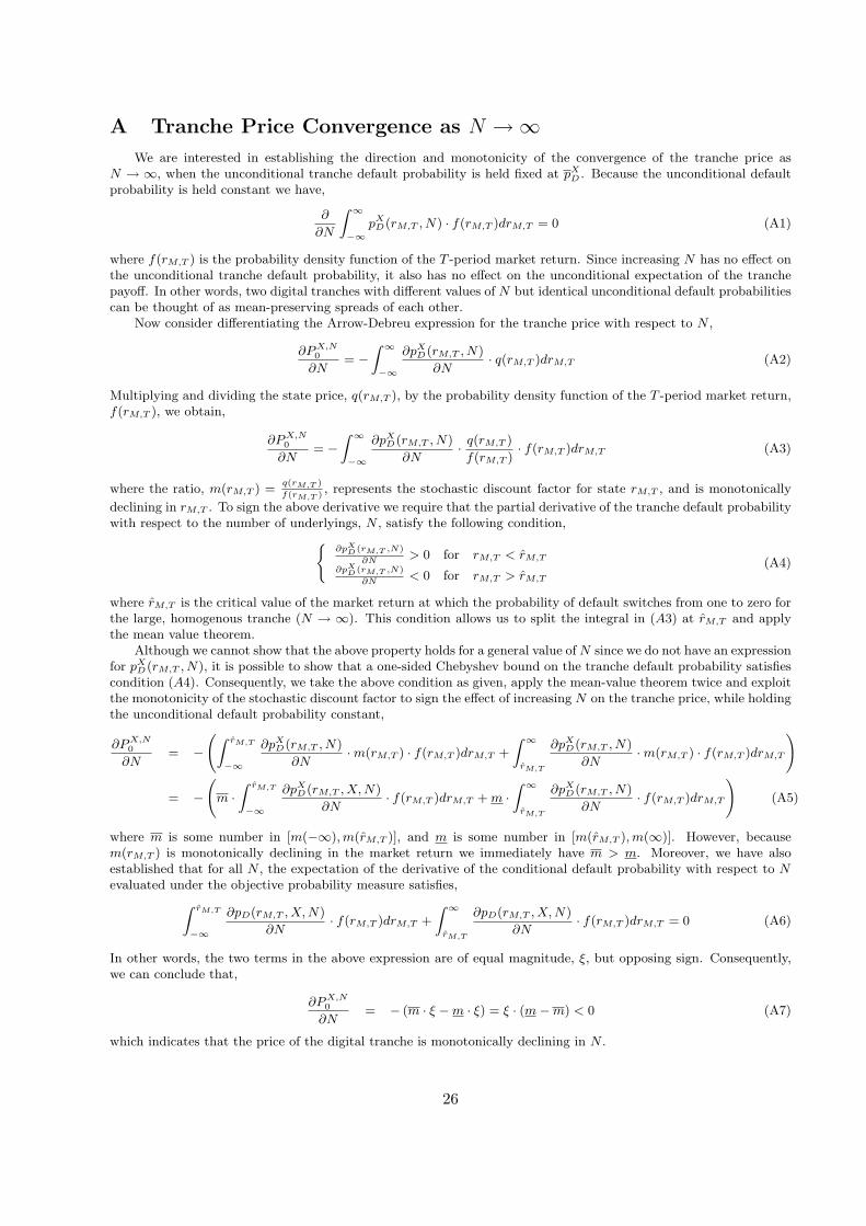
A Tranche Price Convergence as N →∞We are interested in establishing the direction and monotonicity of the convergence of the tranche price as

N → ∞, when the unconditional tranche default probability is held fixed at pXD . Because the unconditional default

probability is held constant we have,

∂

∂N

Z ∞−∞

pXD(rM,T , N) · f(rM,T )drM,T = 0 (A1)

where f(rM,T ) is the probability density function of the T -period market return. Since increasing N has no effect onthe unconditional tranche default probability, it also has no effect on the unconditional expectation of the tranchepayoff. In other words, two digital tranches with different values of N but identical unconditional default probabilitiescan be thought of as mean-preserving spreads of each other.

Now consider differentiating the Arrow-Debreu expression for the tranche price with respect to N ,

∂P X,N0

∂N= −

Z ∞−∞

∂pXD(rM,T , N)

∂N· q(rM,T )drM,T (A2)

Multiplying and dividing the state price, q(rM,T ), by the probability density function of the T -period market return,f(rM,T ), we obtain,

∂P X,N0

∂N= −

Z ∞−∞

∂pXD(rM,T , N)

∂N· q(rM,T )

f(rM,T )· f(rM,T )drM,T (A3)

where the ratio, m(rM,T ) =q(rM,T )

f(rM,T ), represents the stochastic discount factor for state rM,T , and is monotonically

declining in rM,T . To sign the above derivative we require that the partial derivative of the tranche default probabilitywith respect to the number of underlyings, N , satisfy the following condition,(

∂pXD (rM,T ,N)

∂N> 0 for rM,T < r̂M,T

∂pXD (rM,T ,N)

∂N< 0 for rM,T > r̂M,T

(A4)

where r̂M,T is the critical value of the market return at which the probability of default switches from one to zero forthe large, homogenous tranche (N → ∞). This condition allows us to split the integral in (A3) at r̂M,T and applythe mean value theorem.

Although we cannot show that the above property holds for a general value of N since we do not have an expressionfor pX

D(rM,T , N), it is possible to show that a one-sided Chebyshev bound on the tranche default probability satisfiescondition (A4). Consequently, we take the above condition as given, apply the mean-value theorem twice and exploitthe monotonicity of the stochastic discount factor to sign the effect of increasing N on the tranche price, while holdingthe unconditional default probability constant,

∂P X,N0

∂N= −

Z r̂M,T

−∞

∂pXD(rM,T , N)

∂N·m(rM,T ) · f(rM,T )drM,T +

Z ∞r̂M,T

∂pXD(rM,T , N)

∂N·m(rM,T ) · f(rM,T )drM,T

!

= −

m ·

Z r̂M,T

−∞

∂pXD(rM,T , X, N)

∂N· f(rM,T )drM,T + m ·

Z ∞r̂M,T

∂pXD(rM,T , N)

∂N· f(rM,T )drM,T

!(A5)

where m is some number in [m(−∞), m(r̂M,T )], and m is some number in [m(r̂M,T ), m(∞)]. However, becausem(rM,T ) is monotonically declining in the market return we immediately have m > m. Moreover, we have alsoestablished that for all N , the expectation of the derivative of the conditional default probability with respect to Nevaluated under the objective probability measure satisfies,Z r̂M,T

−∞

∂pD(rM,T , X, N)

∂N· f(rM,T )drM,T +

Z ∞r̂M,T

∂pD(rM,T , X, N)

∂N· f(rM,T )drM,T = 0 (A6)

In other words, the two terms in the above expression are of equal magnitude, ξ, but opposing sign. Consequently,we can conclude that,

∂P X,N0

∂N= − (m · ξ −m · ξ) = ξ · (m−m) < 0 (A7)

which indicates that the price of the digital tranche is monotonically declining in N .

26

B Fitting the Implied Volatility Smile

We consider two parametric forms for the implied volatility function when fitting the prices of five-year S&P 500index options:

σt(x, T ) = a + b · exp(−c · x) (B1)

σt(x, T ) = a + b · tanh(−c · ln x) (B2)

where x is the option moneyness, defined as the ratio of the option strike price to the prevailing spot price. Thesefunctional forms for the volatility skew have a variety of attractive features. First, they can generate an approximatelylinear skew for options whose strike prices are close to at-the-money, matching the stylized facts for long-dated options.Second, the functions are bounded above and below, allowing us to control the magnitude of the implied volatilityoutside of the domain of strike prices for which we observe option prices. This approach is more elegant than assuminga constant implied volatility outside the range of observable option prices (Shimko (1993), Campa et al. (1997))),since it avoids problems of non-differentiability and ensures that prices are martingales. The solution proposed byBrown and Toft (1999) is most similar to ours. They assume that the implied volatility function converges to someexogenously specified value. Instead, we “fit” this asymptotic value by requiring that the implied risk-neutral densityallow us to consistently price a riskless bond and a futures contract (i.e. an option with a strike of K = 0). Lastly, thesimple parametric forms we chose facilitate the analytical computation of the derivatives appearing in the formulafor the Arrow-Debreu prices.

For example, for the exponential implied volatility function, the first and second derivatives of the impliedvolatility function with respect to the strike price (or, equivalently, moneyness) are given by:

dσt(x, T )

dx= −bc · exp(−c · x) (B3)

d2σt(x, T )

dx2= bc2 · exp(−c · x) (B4)

The corresponding derivatives for the hyperbolic tangent implied volatility function are:

dσt(x, T )

dx=

„b · cx

«· sech2(c · ln x) (B5)

d2σt(x, T )

dx2= −

„b · cx2

«· sech3(c · ln x) · (cosh(c · ln x) + 2c · sinh(c · ln x)) (B6)

The remainder of the partial derivatives appearing in formula for the Arrow-Debreu state prices can be obtainedby differentiating the Black-Scholes formula with respect to its various parameters. In particular, we obtain:

∂2Ct

∂K2

˛̨̨̨x

= e−rT · φ(d2(x))

xσt(x, T )√

T(B7)

∂Ct

∂σ

˛̨̨̨x

= φ(d1(x)) ·√

T = e−rT · x · φ(d2(x)) ·√

T (B8)

∂2Ct

∂σ2

˛̨̨̨x

=d1(x) · d2(x)

σt(x, T )· φ(d1(x)) ·

√T = e−rT · x · d1(x) · d2(x)

σt(x, T )· φ(d2(x)) ·

√T (B9)

∂Ct

∂K∂σ

˛̨̨̨x

=2d1(x) · φ(d1(x))

x · σt(x, T )= e−rT · 2d1(x) · φ(d2(x))

σt(x, T )(B10)

where:

d1(x) =ln 1

x+`rf + 1

2· σt(x, T )2

´· T

σt(x, T ) ·√

T(B11)

d2(x) = d1 − σt(x, T ) ·√

T (B12)

Substituting these expressions back into the formula for the Arrow-Debreu prices, yields a closed-from representationfor the state prices implied by our parametrization of the implied volatility function.

27

28

Table 1 Summary Statistics for US Credit Market (9/2004 – 9/2006)

This table reports summary statistics of various credit market securities. The 5-year bond-implied CDS spreads by rating group are provided by Lehman Brothers. The CDX series is the Dow Jones CDX North America Investment Grade index of 5-year credit default swaps. The CDX tranche spreads are denoted as [lower loss attachment, upper loss attachment]. The VIX is the Chicago Board Options Exchange (CBOE) volatility index measuring near-term implied volatility from S&P500 index options. Five-year at-the-money implied volatility is denoted as 5yVol. The skew is the linear slope between 5-year at-the-money volatility and 5-year 30% out-of-the-money volatility. The yield on 5-year constant maturity Treasury bonds is denoted Rf.

Panel A: Time series means and standard deviations of daily series in basis points (volatility in percent) VIX 5yVOL Skew Rf AA A BBB BB B CDX [3-7] [7-10] [10-15] [15-30]

Mean 13.2 17.8 -12.8 4.2 15.3 25.6 46.9 143.1 254.5 47.8 146.2 44.0 19.8 9.2 Std 1.8 1.3 0.8 0.5 2.2 2.6 5.5 22.9 36.8 6.9 56.5 24.8 9.0 3.7 Panel B: Correlations between weekly series

VIX 5yVOL Skew Rf AA A BBB BB B CDX [3-7] [7-10] [10-15] [15-30]VIX 1.00 5yVOL 0.38 1.00 Skew 0.23 0.00 1.00 Rf 0.17 0.58 0.25 1.00 AA -0.02 0.55 0.05 0.40 1.00 A -0.11 0.14 -0.15 -0.38 0.27 1.00 BBB 0.04 0.52 -0.11 -0.14 0.54 0.85 1.00 BB 0.24 0.63 -0.40 -0.01 0.28 0.57 0.73 1.00 B -0.06 0.39 -0.50 -0.23 0.24 0.72 0.76 0.85 1.00 CDX 0.07 -0.14 -0.53 -0.63 -0.22 0.52 0.39 0.52 0.64 1.00 [3-7] 0.18 -0.43 -0.05 -0.83 -0.48 0.32 0.13 0.08 0.20 0.66 1.00 [7-10] 0.12 -0.49 0.05 -0.86 -0.44 0.27 0.10 -0.08 0.05 0.53 0.96 1.00 [10-15] 0.10 -0.46 -0.12 -0.89 -0.43 0.39 0.19 0.09 0.22 0.72 0.96 0.96 1.00 [15-30] -0.03 -0.32 -0.39 -0.66 -0.39 0.51 0.26 0.33 0.46 0.89 0.69 0.60 0.77 1.00 Panel C: Correlations between changes in weekly series

VIX 5yVOL Skew Rf AA A BBB BB B CDX [3-7] [7-10] [10-15] [15-30]VIX 1.00 5yVOL 0.46 1.00 Skew 0.03 -0.09 1.00 Rf -0.09 0.06 -0.07 1.00 AA -0.01 -0.05 -0.04 -0.20 1.00 A -0.15 -0.05 0.04 -0.26 0.71 1.00 BBB -0.07 0.11 -0.02 -0.36 0.63 0.85 1.00 BB 0.27 0.18 -0.06 -0.57 0.24 0.33 0.47 1.00 B 0.25 0.22 0.05 -0.48 0.22 0.34 0.45 0.77 1.00 CDX 0.38 0.26 -0.03 -0.13 -0.02 -0.01 0.10 0.47 0.37 1.00 [3-7] 0.12 0.19 -0.15 0.00 0.17 0.21 0.27 0.48 0.43 0.49 1.00 [7-10] 0.09 0.12 -0.15 -0.02 0.17 0.17 0.22 0.30 0.28 0.46 0.84 1.00 [10-15] 0.16 0.15 -0.15 -0.10 0.18 0.15 0.25 0.39 0.31 0.58 0.80 0.82 1.00 [15-30] 0.13 0.16 -0.10 -0.02 0.02 0.08 0.12 0.35 0.28 0.58 0.65 0.62 0.77 1.00

29

Table 2 Regressions Explaining the Time Series of Changes in CDX Yield Spreads (9/2004 – 9/2006)

The dependent variable is the weekly change in the CDX yield spread. The CDX series is the Dow Jones CDX North America Investment Grade index of 5-year credit default swaps. The model predicted change in the CDX yield spread, E[ΔYCDX,Exp] and E[ΔYCDX,Tanh], is calculated as the difference between the model yield at time t+1, using parameters calibrated at time t, and the actual yield at time t, using the exponential and hyperbolic tangent implied volatility state price densities, respectively. The yield on 5-year constant maturity Treasury bonds is denoted Rf. S&P refers to the level of the S&P 500 index. Five-year at-the-money implied volatility is denoted as 5yVol. The skew is the linear slope between 5-year at-the-money volatility and 5-year 30% out-of-the-money volatility. The adjusted R-square is denoted R2, t-statistics are in parenthesis, and the number of observations are in square brackets.

Intercept E[ΔYCDX, Exp]

E[ΔYCDX, Tanh] ΔRf ΔS&P Δ5yVol ΔSkew R2 [N]

0.0000 0.2702 0.3455 (-0.29) (7.19) [97]

0.0000 0.2445 0.3249 (-0.28) (6.87) [97]

0.0000 -0.0555 0.0324 (-0.31) (-2.05) [97]

0.0000 -0.0092 0.2309 (-0.03) (-5.46) [97]

0.0000 0.0285 0.1852 (-0.84) (4.78) [97]

0.0000 0.0529 0.0060 (-0.62) (1.26) [97]

0.0000 -0.0275 -0.0068 0.0147 0.0537 0.2858 (-0.13) (-1.16) (-3.60) (2.23) (1.49) [97]

0.0000 0.5430 0.0215 0.0071 -0.0134 -0.0462 0.3291 (-0.44) (2.39) (0.68) (1.24) (-1.08) (-0.92) [97]

0.0000 0.3916 0.0080 0.0044 -0.0080 0.0285 0.3106 (-0.35) (1.76) (0.25) (0.71) (-0.61) (0.85) [97]

30

Table 3 Comparison of Actual and Model Implied Tranche Spreads

The actual weekly CDX tranche spreads corresponds to various tranches of the Dow Jones CDX North America Investment Grade index of 5-year credit default swaps. The model yield is calculated a Merton (1974) / CAPM credit model calibration procedure. The credit risk ratio, λQ/λP, for the tranches is calculated by dividing the model yield spread by the loss rate (i.e. the yield spread that would be obtained by discounting at the riskfree rate). The mean 5-year default probability is calculated using the time series average of the weekly objective default intensity. Panel A: Model assumes continuum of index option strikes

Tranche Mean Model Spread [bps]

Mean Actual Spread [bps]

Correlation of Model and

Actual

Correlation of Model and

Actual (Changes)

Mean 5-Year Default

Probability (%)

Mean λQ / λP

Exponential Implied Volatility Function 3%-7% 184 147 0.78 0.44 4.37 5.3 7%-10% 110 44 0.40 0.39 0.57 18.2 10%-15% 78 20 0.42 0.51 0.17 59.3 15%-30% 44 9 0.50 0.37 0.03 576.5

Hyperbolic Tangent Implied Volatility Function 3%-7% 215 147 0.58 0.54 5.55 4.6 7%-10% 124 44 0.22 0.44 0.76 15.0 10%-15% 80 20 0.40 0.51 0.23 44.6 15%-30% 34 9 0.71 0.35 0.04 330.8

Panel B: Model assumes a static index put spread is available at each CDX initiation date

Tranche Mean Model Spread [bps]

Mean Actual Spread [bps]

Correlation of Model and

Actual

Correlation of Model and

Actual (Changes)

Mean 5-Year Default

Probability (%)

Mean λQ / λP

Exponential Implied Volatility Function 3%-7% 200 147 0.19 0.56 3.72 5.6 7%-10% 115 44 0.22 0.32 0.41 22.2 10%-15% 82 20 0.31 0.49 0.15 72.0 15%-30% 47 9 0.30 0.28 0.03 576.5

Hyperbolic Tangent Implied Volatility Function 3%-7% 234 147 0.20 0.53 4.50 5.0 7%-10% 130 44 0.26 0.31 0.52 18.4 10%-15% 85 20 0.33 0.50 0.19 53.1 15%-30% 37 9 0.25 0.20 0.04 308.5

31

Table 4 Yields on Various S&P 500 Put Spreads

The yield on the 5-year S&P 500 put spread is calculated for a variety of strike prices. The put spread consists of shorting an index put option at the upper strike price and buying an index put option at the lower strike price. Panel A reports the average daily yield for various put spreads assuming an exponential implied volatility function. Panel B reports the average daily yield for various put spreads assuming a hyperbolic tangent implied volatility function. Panel C reports the daily yield for various put spreads on September 11, 2006, assuming an exponential implied volatility function. Panel D reports the daily yield for various put spreads on September 11, 2006, assuming a hyperbolic tangent implied volatility function.

Average Daily Yield from 9/2004 to 9/2006 Panel A: Exponential Implied Volatility Function Upper Strike Price 0.30 0.35 0.40 0.45 0.50 0.55 0.60 0.65 0.70 0.75

0.00 17 22 28 34 42 50 59 68 80 920.05 20 26 32 39 46 55 64 74 86 990.10 24 30 37 44 52 61 70 81 93 1060.15 29 36 43 50 58 67 77 88 101 1150.20 35 42 49 56 65 74 85 96 109 1240.25 41 48 55 63 72 82 93 105 118 1330.30 55 62 71 80 90 101 114 128 1440.35 70 79 88 99 111 124 139 1550.40 88 98 109 121 135 150 1680.45 108 119 132 147 163 1810.50 131 145 160 177 1960.55 159 175 193 2130.60 191 210 2320.65 230 252

Low

er S

trik

e P

rice

0.70 275 Panel B: Hyperbolic Tangent Implied Volatility Function Upper Strike Price 0.30 0.35 0.40 0.45 0.50 0.55 0.60 0.65 0.70 0.75

0.00 8 13 19 27 35 44 55 66 78 910.05 10 15 22 30 39 49 60 71 84 980.10 12 18 26 34 44 54 66 78 91 1060.15 16 23 31 40 50 61 73 86 99 1150.20 21 28 37 47 57 69 81 95 109 1250.25 27 35 45 55 66 78 91 105 120 1360.30 44 54 64 76 89 102 116 132 1490.35 64 75 87 100 114 129 145 1620.40 86 99 112 127 142 158 1770.45 112 125 140 156 173 1920.50 139 155 171 189 2080.55 170 187 206 2260.60 204 224 2450.65 243 266

Low

er S

trik

e P

rice

0.70 288

32

Table 4 (Continued)

Yield on 9/11/2006 Panel C: Exponential Implied Volatility Function Upper Strike Price 0.30 0.35 0.40 0.45 0.50 0.55 0.60 0.65 0.70 0.75

0.00 15 21 28 35 44 54 64 76 90 1040.05 18 24 32 40 49 59 70 83 97 1120.10 22 29 37 45 55 66 77 90 105 1210.15 27 35 43 52 62 73 85 99 114 1300.20 33 41 50 60 70 82 94 108 124 1410.25 41 49 58 68 79 91 104 119 135 1530.30 57 67 77 89 101 115 130 147 1660.35 76 87 99 112 127 143 160 1800.40 98 111 125 140 156 175 1950.45 123 138 154 171 190 2120.50 152 169 187 208 2300.55 186 205 226 2490.60 224 247 2710.65 269 295

Low

er S

trik

e P

rice

0.70 321 Panel D: Hyperbolic Tangent Implied Volatility Function Upper Strike Price 0.30 0.35 0.40 0.45 0.50 0.55 0.60 0.65 0.70 0.75

0.00 7 13 20 28 38 49 61 74 88 1040.05 9 15 23 32 42 54 67 80 95 1110.10 11 18 27 37 48 60 73 88 103 1200.15 14 22 32 43 55 68 82 97 113 1300.20 20 28 39 50 63 77 92 107 124 1420.25 27 36 48 60 73 88 103 119 137 1560.30 46 58 71 85 100 116 133 151 1700.35 70 84 98 114 130 148 166 1860.40 98 113 129 146 164 183 2040.45 128 144 162 180 200 2220.50 161 179 198 219 2410.55 197 217 238 2610.60 237 259 2830.65 282 307

Low

er S

trik

e P

rice

0.70 332 Credit Market Summary on 9/11/2006 in basis points (volatility in percent)

VIX 5yVOL AA A BBB BB B CDX 3-7 7-10 10-15 15-30

Mean 13.0 19.3 15.9 28.1 52.5 158.9 264.1 37.3 71.5 15.5 7.5 4.0

33

Figure 1. Time series of the 7%-10% tranche spread and credit spreads for bond indices (9/2004 – 9/2006). The AA and BBB 5-year bond-implied CDS spreads are provided by Lehman Brothers. The CDX tranche spread corresponds to the 7%-10% tranche of the Dow Jones CDX North America Investment Grade index of 5-year credit default swaps.

34

0 0.5 1.0 1.5 2.0 2.5 3.0 3.50

0.1

0.2

0.3

0.4

Moneyness

Pric

e ($

)

Calibrated 5-Year Option Implied State Prices

0.0 0.5 1.0 1.5 2.0 2.5 3.0 3.5

10

20

30

40

Moneyness

(%)

Calibrated 5-Year Implied Volatility Function

Series 3Series 4Series 5Series 6

Series 3Series 4Series 5Series 6

Figure 2. Calibrated 5-year state prices and implied volatility functions as of CDX initiation dates. Panel A: Exponential implied volatility function. The top panel displays state prices calculated using the technique of Breeden and Litzenberger (1978), adjusted to account for the implied volatility skew. The bottom panel shows the parametric implied volatility function fitted using prices of 5-year S&P 500 index options. The observed option prices come from securities with normalized strike prices ranging from 0.70 to 1.30, at 0.05 increments.

35

0 0.5 1.0 1.5 2.0 2.5 3.0 3.50

0.1

0.2

0.3

0.4

Moneyness

Pric

e ($

)

Calibrated 5-Year Option Implied State Prices

0.0 0.5 1.0 1.5 2.0 2.5 3.0 3.50

10

20

30

Moneyness

(%)

Calibrated 5-Year Implied Volatility Function

Series 3Series 4Series 5Series 6

Series 3Series 4Series 5Series 6

Figure 2. Calibrated 5-year state prices and implied volatility functions as of CDX initiation dates. Panel B: Hyperbolic tangent implied volatility function. The top panel displays state prices calculated using the technique of Breeden and Litzenberger (1978), adjusted to account for the implied volatility skew. The bottom panel shows the parametric implied volatility function fitted using prices of 5-year S&P 500 index options. The observed option prices come from securities with normalized strike prices ranging from 0.70 to 1.30, at 0.05 increments.

36

4 5 60

10

20

30

40

50

60

70

80

Series

[bps

][Mean Intensity = 19.9bps; Mean Yield = 43.0bps]

Default IntensityYield

4 5 60

2

4

6

8

10

Series

λQ / λP

[Mean Ratio = 3.8]

λQ / λP

Figure 3. Time series of calibrated CDX default intensity and spread. The CDX yield, yCDX, is given by the Dow Jones CDX North America Investment Grade index of 5-year credit default swaps. Each day, the Merton (1974) structural credit model is applied to 125 identical CAPM assets to determine the CDX default rate conditional on the market return. The conditional payoff for the CDX is calculated using a recovery rate, R, of 40%. The conditional payoff is priced with a market index option implied state price density, constructed from a fitted exponential implied volatility function. To calculate the objective default intensity, λP, we assume the terminal value of the market index is lognormal. The risk-neutral default intensity, λQ, is calculated as yCDX/(1-R).

37

Figure 4. State Contingent CDX default rate, CDX payoff, and the 7%-10% tranche payoff. The top panel of the figure plots the calibrated firm default rate as a function of the 5-year market return. The default rate characterizes the representative bond in the credit default index (CDX). The figure includes a sample of the CDX payoff realizations (blue dots) and their state contingent mean (red line). The payoffs are obtained via Monte Carlo simulation using calibrated firm parameters as of the last date in the sample. The mean recovery rate conditional on default is fixed at 40% of par. The bottom panel plots the corresponding payoffs to the 7%-10% tranche (blue dots) and their state-contingent mean (red line). The dashed black line depicts the payoff to an approximating put spread portfolio.

38

4 5 650

100

150

200

250

300

350

Series

Spr

ead

[bps

]

Model 3-7

Figure 5. Time series of actual and model tranche spread (9/2004 – 9/2006). The actual CDX tranche spread corresponds to the 3%-7% tranche on the Dow Jones CDX North America Investment Grade index of 5-year credit default swaps. The model yield is estimated by first applying the Merton (1974) credit model to 125 identical CAPM assets to determine the CDX default rate conditional on the market return. The conditional payoff for the CDX is calculated using a recovery rate, R, of 40%. The conditional payoff is priced with a market index option implied state price density, constructed from a fitted exponential implied volatility function. The model parameters are calibrated such that the model CDX yield matches the observed CDX yield. The conditional payoff for the tranche is simulated using the calibrated CDX parameters and priced using the state price density.

39

4 5 60

20

40

60

80

100

120

140

160

180

200

Series

Spr

ead

[bps

]

Model 7-10

Figure 6. Time series of actual and model tranche spread (9/2004 – 9/2006). The actual CDX tranche spread corresponds to the 7%-10% tranche on the Dow Jones CDX North America Investment Grade index of 5-year credit default swaps. The model yield is estimated by first applying the Merton (1974) credit model to 125 identical CAPM assets to determine the CDX default rate conditional on the market return. The conditional payoff for the CDX is calculated using a recovery rate, R, of 40%. The conditional payoff is priced with a market index option implied state price density, constructed from a fitted exponential implied volatility function. The model parameters are calibrated such that the model CDX yield matches the observed CDX yield. The conditional payoff for the tranche is simulated using the calibrated CDX parameters and priced using the state price density.

40

4 5 60

20

40

60

80

100

120

140

Series

Spr

ead

[bps

]

Model10-15

Figure 7. Time series of actual and model tranche spread (9/2004 – 9/2006). The actual CDX tranche spread corresponds to the 10%-15% tranche on the Dow Jones CDX North America Investment Grade index of 5-year credit default swaps. The model yield is estimated by first applying the Merton (1974) credit model to 125 identical CAPM assets to determine the CDX default rate conditional on the market return. The conditional payoff for the CDX is calculated using a recovery rate, R, of 40%. The conditional payoff is priced with a market index option implied state price density, constructed from a fitted exponential implied volatility function. The model parameters are calibrated such that the model CDX yield matches the observed CDX yield. The conditional payoff for the tranche is simulated using the calibrated CDX parameters and priced using the state price density.

41

4 5 60

10

20

30

40

50

60

70

80

Series

Spr

ead

[bps

]

Model15-30

Figure 8. Time series of actual and model tranche spread (9/2004 – 9/2006). The actual CDX tranche spread corresponds to the 15%-30% tranche on the Dow Jones CDX North America Investment Grade index of 5-year credit default swaps. The model yield is estimated by first applying the Merton (1974) credit model to 125 identical CAPM assets to determine the CDX default rate conditional on the market return. The conditional payoff for the CDX is calculated using a recovery rate, R, of 40%. The conditional payoff is priced with a market index option implied state price density, constructed from a fitted exponential implied volatility function. The model parameters are calibrated such that the model CDX yield matches the observed CDX yield. The conditional payoff for the tranche is simulated using the calibrated CDX parameters and priced using the state price density.

42

0.0%

1.0%

2.0%

3.0%

4.0%

5.0%

6.0%

1987 1988 1989 1990 1991 1992 1993 1994 1995 1996 1997 1998 1999 2000 2001 2002 2003 2004 2005 2006-40%

-30%

-20%

-10%

0%

10%

20%

30%

40%

50%

Downgrade Rate (left axis)

Lagged One-year Market Returns (right axis)

Correlation = -60%

Figure 9. U.S. Bond Downgrade Rate and Lagged Market Returns (12/1987 – 4/2007). Downgrades correspond to the fraction of publicly-listed US firms with S&P-rated debt that experienced a downgrade during the calendar month. The lagged one-year return corresponds to the cumulative return on the S&P 500 during the past 12 month period. Using individual firm returns, the corresponding logistic regression is estimated as follows:

Prob(Downgradei,t=1)=β

β'exp1

'expX

X+

, where )(' ,,2,10 tmtitm RRbRbbX −⋅+⋅+=β .

The estimated coefficients are displayed in the table below, with p-values reported in parenthesis.

b0 b1 b2 N 3.90 3.27 3.01 129,330

(0.03) (0.13) (0.06)