
Economic Benefits of Lifting the Crude Oil Export Ban - … · Economic Benefits of Lifting the...
196
Economic Benefits of Lifting the Crude Oil Export Ban Prepared for: The Brookings Institution September 9, 2014
Transcript of Economic Benefits of Lifting the Crude Oil Export Ban - … · Economic Benefits of Lifting the...

Economic Benefits of Lifting the Crude Oil Export Ban
Prepared for:
The Brookings Institution
September 9, 2014

Project Team/Authors
Robert Baron
Paul Bernstein
W. David Montgomery
Reshma Patel
Sugandha D. Tuladhar
Mei Yuan
* The authors acknowledge the valuable research support provided by Ryan Jaspal in this project. The authors also thank the Brookings Institution for providing funding for this project and the members of the Brookings Crude Oil Task Force for helping us define the issues to be addressed and access needed data and information. We also would like to thank Porter Bennett, Bernadette Johnson, and Sarp Ozkan of Ponderosa Advisors and Lucian Pugliaresi, President of EPRINC for helping us with data and sharing valuable insights on oil refining and export issues. Our colleague Paul Nicholson at Marsh and Stephen Gordon of Clarkson Research Services, Inc. in London provided us with information on crude oil tanker rates. The opinions expressed herein do not necessarily represent their views or the views of NERA Economic Consulting or any other NERA consultants.
NERA Economic Consulting 1255 23rd Street NW Washington, DC 20037 Tel: +1 202 466 3510 Fax: +1 202 466 3605 www.nera.com

Report Qualifications, Assumptions and Limiting Conditions
The opinions and conclusions stated herein are the sole responsibility of the authors. They do not necessarily represent the views of NERA Economic Consulting or any other NERA consultants or any of NERA’s clients.
Information furnished by others, on which all or portions of this report are based, is believed to be reliable, but has not been independently verified, unless otherwise expressly indicated. Public information and industry and statistical data are from sources we deem to be reliable; however, we make no representation as to the accuracy or completeness of such information. The findings contained in this report may contain predictions based on current data and historical trends. Any such predictions are subject to inherent risks and uncertainties. NERA Economic Consulting accepts no responsibility for actual results or future events.
The opinions expressed in this report are valid only for the purpose stated herein and as of the date of this report. No obligation is assumed to revise this report to reflect changes, events or conditions, which occur subsequent to the date hereof.
All decisions in connection with the implementation or use of advice or recommendations contained in this report are the sole responsibility of the user. This report does not represent investment advice nor does it provide an opinion regarding the fairness of any transaction to any and all parties.
© NERA Economic Consulting

i
Contents
EXECUTIVE SUMMARY ...........................................................................................................1 A. What NERA Was Asked to Do ............................................................................................1 B. NERA’s Approach ...............................................................................................................2 C. Key Findings ........................................................................................................................2
1. Why Lifting the Crude Oil Export Ban Would Yield Positive Economic Impacts .......3 2. The U.S. Economy Will Benefit from Lifting the Crude Oil Export Ban .....................8 3. Consumers Would Benefit from Lifting the Crude Oil Export Ban ............................11 4. How Market Conditions Impact Economic Benefits ...................................................13 5. Lifting the Ban Immediately on all Types of Crude Oil Would Yield the Greatest
Economic Benefits .......................................................................................................17
I. Introduction ......................................................................................................................19 A. Problem Statement .............................................................................................................20
1. What Would Be the Impacts on the Domestic and International Energy Markets Resulting from the U.S. Lifting its Crude Oil Export Ban? ........................................20
2. What would be the Economic Impacts on the U.S. Economy resulting from Crude Oil Exports? .................................................................................................................21
B. Scope of this Study ............................................................................................................21 C. Organization of this Report ................................................................................................22
II. Description of Global Petroleum Markets and NERA’s Analytical Models ..............23 A. Global Petroleum Markets .................................................................................................23 B. NERA’s Global Petroleum Model .....................................................................................24
1. Crude Oil Transportation: ............................................................................................26 2. Refining: ......................................................................................................................27 3. Refined Petroleum Product Transportation: ................................................................27 4. Consumption: ...............................................................................................................27 5. Refiner’s Options for Increasing the Processing of Domestically Produced Light
Tight Crude Oil ............................................................................................................27 C. NewERA Macroeconomic Model .......................................................................................29 D. Linkage between GPM and NewERA .................................................................................31
III. Description of Scenarios ..................................................................................................33 A. U.S. Crude Oil Market .......................................................................................................33 B. International scenario .........................................................................................................34 C. U.S. regulations pertaining to crude oil exports ................................................................34 D. OPEC response ..................................................................................................................35 E. Summary of all cases .........................................................................................................35
IV. Global Petroleum Model Results ....................................................................................37 A. The NERA U.S. Baseline...................................................................................................37 B. Scenario Results .................................................................................................................38
1. Complete Lifting of the Crude Oil Export Ban in 2015 ..............................................39 2. How Market Forces Impact Crude Oil Exports ...........................................................54 3. Alternative Ways to Lift the Crude Oil Export Ban ....................................................59

ii
V. Macroeconomic Impacts .................................................................................................62 A. U.S. Consumer Wellbeing (Welfare) .................................................................................62
1. Immediate lifting of the ban is beneficial to the U.S. consumers: ...............................63 2. Delaying the lifting of the ban reduces net benefit: .....................................................63 3. Partial lifting of the ban provides smaller benefit: .......................................................64 4. Change in OPEC responses does not alter net benefits to the U.S. economy: ............65 5. With lower world oil demand, the U.S. economy still benefits from exporting
crude oil: ......................................................................................................................66 6. Summary: Immediate lifting of the ban on all crude oil exports results in the
greatest economic benefits for the U.S.: ......................................................................67 B. Aggregate consumption .....................................................................................................68 C. Investment ..........................................................................................................................72 D. Gross Domestic Product ....................................................................................................75 E. Impact on Labor Markets ...................................................................................................82
1. Change in labor income ...............................................................................................82 2. Change in Real Wages .................................................................................................83
F. Reduction in Unemployment .............................................................................................87 1. Transitional Unemployment ........................................................................................87 2. Okun’s Law and the Relationship between GDP Growth and Unemployment...........88
G. Industrial Output ................................................................................................................91 H. The Value-Added Fallacy ..................................................................................................92 I. Emissions ...........................................................................................................................94
APPENDIX A: TABLES OF ASSUMPTIONS AND NON-PROPRIETARY DATA FOR THE GLOBAL PETROLEUM MODEL .............................................................96
A. Region Assignment ............................................................................................................96 B. Time Horizon .....................................................................................................................98 C. Crude Oil Production .........................................................................................................98
1. U.S. ..............................................................................................................................98 2. Canada..........................................................................................................................98 3. Outside North America ................................................................................................99
D. Crude Oil Wellhead Prices ...............................................................................................102 1. U.S. ............................................................................................................................102 2. Canada........................................................................................................................103 3. Outside North America ..............................................................................................103
E. Refined Petroleum Product Consumption .......................................................................105 1. U.S. ............................................................................................................................106 2. Canada........................................................................................................................106 3. Outside North America ..............................................................................................106
F. Refined Petroleum Product Consumption Prices .............................................................108 1. U.S. ............................................................................................................................109 2. Canada........................................................................................................................109 3. Outside North America ..............................................................................................109
G. Refinery Inputs.................................................................................................................111 H. Costs to Move Products ...................................................................................................116
1. Pipeline ......................................................................................................................116 2. Rail .............................................................................................................................118

iii
3. Barge ..........................................................................................................................118 I. Elasticity ..........................................................................................................................120
APPENDIX B: DESCRIPTION OF MODELS .....................................................................121 A. Global Petroleum Model ..................................................................................................121
1. Model Calibration ......................................................................................................121 2. Model Formulation ....................................................................................................121
B. NewERA Model ................................................................................................................126 1. Overview of the NewERA Macroeconomic Model ....................................................126 2. Model Data (IMPLAN and EIA) ...............................................................................126 3. Brief Discussion of Model Structure .........................................................................126
APPENDIX C: TABLES AND MODEL RESULTS .............................................................137 A. Global Petroleum Model ..................................................................................................137 B. NewERA Model Results ...................................................................................................156
APPENDIX D: TABLE OF SCENARIOS ..............................................................................172
APPENDIX E: REFINERY PROJECT AND OWNERSHIP TABLES ..............................173

iv
List of Figures
Figure 1: Incremental Crude Oil Production Resulting from the Complete Lifting of the Crude Oil Export Ban in 2015 (Ref and HOGR Baselines: MBD) .............................................. 4
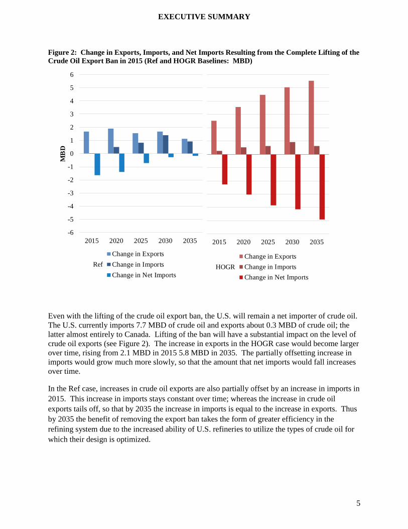
Figure 2: Change in Exports, Imports, and Net Imports Resulting from the Complete Lifting of the Crude Oil Export Ban in 2015 (Ref and HOGR Baselines: MBD) ............................. 5
Figure 3: Change in Average Rest of World Crude Oil Price Resulting from the Complete Lifting of the Crude Oil Export Ban in 2015 (Ref and HOGR Baselines: $/bbl) .............. 6
Figure 4: Change in the U.S. Gasoline Price Resulting from the Complete Lifting of the Ban in 2015 (Ref and HOGR Baselines: $/gal)............................................................................. 7
Figure 5: Historical U.S. Refinery Gross Margin and Forecasted U.S. Refinery Gross Margins under Different Assumptions about the U.S. Crude Oil Export Ban and Availability of U.S. Crude Oil Resources (Ref and HOGR Baselines: $/bbl) ........................................... 8
Figure 6: Range of Change in U.S. Welfare Resulting from the Partial or Complete Lifting of the Crude Oil Export Ban (Ref and HOGR Baselines: %) ................................................ 9
Figure 7: Range of Change in Net Present Value of GDP Resulting from the Partial or Complete Lifting of the Crude Oil Export Ban (Ref and HOGR Baselines: Billion $) ................... 10
Figure 8: Range of Change in Real Wages in 2015 and 2035 Resulting from the Partial or Complete Lifting of the Crude Oil Export Ban (Ref and HOGR Baselines: %) ............. 11
Figure 9: Range of Change in U.S. Gasoline Prices in 2015 and 2035 Resulting from the Partial or Complete Lifting of the Crude Oil Export Ban (Ref and HOGR Baselines: $/gal) .... 12
Figure 10: Average Annual Reduction in Unemployment (2015 – 2020) Resulting from the Lifting of the Crude Oil Export Ban in 2015 versus 2020 (Ref and HOGR Baselines) ... 13
Figure 11: Change in Net Present Value of U.S. GDP Resulting from a Complete Lifting of the Ban in 2015 under Different Assumptions about OPEC’s Actions (Ref and HOGR Baselines: Billion $) ......................................................................................................... 14
Figure 12: Change in OPEC’s Exports of Crude Oil Resulting from a Complete Lifting the Ban in 2015 under Different Assumptions about OPEC’s Actions (Ref and HOGR Baselines: %) ...................................................................................................................................... 15
Figure 13: Change in Net Present Value of U.S. GDP Resulting from a Complete Lifting of the Ban in 2015 (Ref and Ref with LowAP Baselines: Billion $) ......................................... 16
Figure 14: Change in Net Present Value of Welfare Resulting from a Complete Lifting of the Ban in 2015 compared to a Complete Lifting of the Ban in 2020 and Lifting of the Ban on only Condensates (Ref and HOGR Baselines: Billion $) ........................................... 17

v
Figure 15: GPM’s Representation of the Crude and Refined Oil Value Chain ........................... 25
Figure 16: API Gravities of Crude Oil Types Considered in this Report ..................................... 26
Figure 17: Data Transfer between the NERA’s Global Petroleum and NewERA Models ........... 32
Figure 18: Reduction in Asia Pacific’s Demand for Refined Petroleum Products (LowAP Baseline: %) ..................................................................................................................... 34
Figure 19: Summary of Scenarios Analyzed in this Study .......................................................... 36
Figure 20: NERA’s Ref Baseline for U.S. Crude Oil Production, Average Wellhead Crude Oil Price, and Demand for Refined Petroleum Products ........................................................ 37
Figure 21: NERA’s HOGR Baseline for U.S. Crude Oil Production, Average Wellhead Crude Oil Price, and Demand for Refined Petroleum Products .................................................. 38
Figure 22: U.S. ICRU-U.S. LTO Price Spread with and without the Crude Oil Export Ban in Place (Ref Baseline: 2013$/bbl) ...................................................................................... 40
Figure 23: U.S. ICRU-U.S. LTO Price Spread with and without the Crude Oil Export Ban in Place (HOGR Baseline: 2013$/bbl) ................................................................................. 41
Figure 24: International LTO-U.S. LTO Price Spread with and without the Crude Oil Export Ban in Place (Ref Baseline: 2013$/bbl) ........................................................................... 42
Figure 25: International LTO-U.S. LTO Price Spread with and without the Crude Oil Export Ban in Place (HOGR Baseline: 2013$/bbl) ...................................................................... 43
Figure 26: Incremental Crude Oil Production Resulting from the Complete Lifting of the Crude Oil Export Ban in 2015 (Ref and HOGR Baselines: MBD) ............................................ 44
Figure 27: Distribution of Incremental Crude Oil Production by PADD in 2015 Resulting from the Complete Lifting of the Crude Oil Export Ban in 2015 (Ref and HOGR Baselines: MBD) ................................................................................................................................ 45
Figure 28: Change in Crude Oil Export and Imports Resulting from the Complete Lifting of the Crude Oil Export Ban in 2015 (Ref Baseline: MBD) ...................................................... 46
Figure 29: Change in Crude Oil Export and Imports Resulting from the Complete Lifting of the Ban in 2015 (HOGR Baseline: MBD) ............................................................................. 47
Figure 30: Waterfall Chart Showing the Change in U.S. Exports, Imports, Consumption and Production of Crude Oil Resulting from the Complete Lifting of the Ban in 2015 (Ref Baseline: MBD) ............................................................................................................... 48
Figure 31: Waterfall Chart Showing the Change in U.S. Exports, Imports, Consumption and Production of Crude Oil Resulting from the Complete Lifting of the Ban in 2015 (HOGR Baseline: MBD) ............................................................................................................... 48

vi
Figure 32: Change in Average Crude Oil Price for Rest of World from the Complete Lifting of the Ban in 2015 (Ref and HOGR Baselines: 2013$/bbl) ................................................. 49
Figure 33: Distribution of U.S. Crude Oil Exports in the World Market Resulting from the Complete Lifting of the Ban in 2015 (Ref and HOGR Baselines: MBD) ....................... 50
Figure 34: Change in the U.S. Gasoline Prices Resulting from the Complete Lifting of the Ban in 2015 (Ref and HOGR Baselines: 2013$/gal) .............................................................. 51
Figure 35: Change in U.S. Refined Petroleum Product Exports and Imports Resulting from the Complete Lifting of the Ban in 2015 (Ref and HOGR Baselines: MBD) ....................... 52
Figure 36: Historical U.S. Refinery Gross Margin and Forecasted U.S. Refinery Gross Margins under Different Assumptions about the U.S. Crude Oil Export Ban and Availability of U.S. Crude Oil Resources (Ref and HOGR Baselines: 2013$/bbl) ................................ 53
Figure 37: Annualized OPEC Revenues from Petroleum Exports (Ref Baseline: Billion 2013$s)........................................................................................................................................... 54
Figure 38: Annualized OPEC Revenues from Petroleum Exports (HOGR Baseline: Billion 2013$s) .............................................................................................................................. 55
Figure 39: Change in OPEC’s Exports of Crude Oil Resulting from a Complete Lifting of the Ban in 2015 under Different Assumptions about OPEC’s Actions (Ref and HOGR Baselines: %) ................................................................................................................... 56
Figure 40: U.S. Light Tight Crude Oil and Condensate Exports Resulting from the Complete Lifting of the Ban in 2015 (Low Oil Price Baseline: MBD) ........................................... 57
Figure 41: Impact of Completely Lifting the Ban in 2015 as a function of Asia Pacific’s Demand for Refined Petroleum Products (Ref Baseline) ................................................................ 58
Figure 42: Impact of Completely Lifting the Ban in 2015 as a function of Asia Pacific’s Demand for Refined Petroleum Products (HOGR Baseline) ........................................... 58
Figure 43: Comparison between Lifting the Ban on Condensates Alone Versus Lifting the Ban on All Crude Oil Types (Ref Baseline)............................................................................. 60
Figure 44: Comparison between Lifting the Ban on Condensates Alone Versus Lifting the Ban on All Crude Oil Types (HOGR Baseline) ....................................................................... 60
Figure 45: Net Crude Oil Imports Resulting from the Complete Lifting of the Crude Oil Export Ban in 2015 and 2020 (Ref Baseline: MBD) ................................................................... 61
Figure 46: Net Crude Oil Imports Resulting from the Complete Lifting of the Ban in 2015 and 2020 (HOGR Baseline: MBD .......................................................................................... 61

vii
Figure 47: Change in Welfare Resulting from the Complete Lifting of the Ban in 2015 (Ref and HOGR Baselines: %) ....................................................................................................... 63
Figure 48: Change in Welfare Resulting from the Complete Lifting of the Ban in 2015 and 2020 (Ref and HOGR Baselines: %) ........................................................................................ 64
Figure 49: Change in Welfare Resulting from the Complete Lifting of the Ban in 2015 and Lifting of the Ban on Condensates (Ref and HOGR Baselines: %) ................................ 65
Figure 50: Change in Welfare Resulting from the Complete Lifting of the Ban in 2015 under Different OPEC Responses (Ref and HOGR Baselines: %) ........................................... 66
Figure 51: Change in Welfare Resulting from the Complete Lifting of the Ban in 2015 under Different Assumptions about Asia Pacific Demand for Refined Petroleum Products (Ref and HOGR Baselines: %) ................................................................................................ 67
Figure 52: Change in Net Present Value of Welfare Resulting from Complete and Modified Lifting of the Ban under Different Assumptions about OPEC’s Response (Ref and HOGR Baselines: %) ................................................................................................................... 68
Figure 53: Change in Aggregate Consumption Resulting from the Complete Lifting of the Ban in 2015 (Ref and HOGR Baselines: %) ........................................................................... 69
Figure 54: Change in Aggregate Consumption Resulting from the Complete Lifting of the Ban in 2015 (Ref and HOGR Baselines: Billion 2013$) ........................................................ 69
Figure 55: Change in 2015 Income per Household Resulting from the Complete and Partial Lifting of the Ban under Different OPEC Responses (Ref and HOGR Baselines: 2013$ per Household) .................................................................................................................. 70
Figure 56: Change in Aggregate Consumption Resulting from the Complete Lifting of the Ban in 2015 and 2020 (Ref and HOGR Baselines: Billion 2013$) ......................................... 71
Figure 57: Change in Cumulative Net Present Value of Aggregate Consumption between 2015 through 2039 Resulting from the Complete and Partial Lifting of the Ban under Different OPEC Responses (Ref and HOGR Baselines: Billion 2013$) ........................................ 72
Figure 58: Change in Investment Resulting from the Complete Lifting of the Ban in 2015 (Ref and HOGR Baselines: %) ................................................................................................ 73
Figure 59: Percentage Change in 2015 Investment Resulting from the Complete and Partial Lifting of the Ban (Ref and HOGR Baselines: %) .......................................................... 74
Figure 60: Change in Investment Resulting from a Lifting of the Ban under Different Assumptions about OPEC’s Response (Ref Baseline: %) ............................................... 74
Figure 61: Change in Investment Resulting from a Lifting of the Ban under Different Assumptions about OPEC’s Response (HOGR Baseline: %) ......................................... 75

viii
Figure 62: Change in GDP Resulting from the Complete Lifting of the Ban in 2015 (Ref and HOGR Baselines: %) ....................................................................................................... 76
Figure 63: Change in GDP Resulting from the Complete Lifting of the Ban in 2015 (Ref and HOGR Baselines: Billion 2013$) .................................................................................... 77
Figure 64: Range of Change in U.S. GDP Resulting from the Partial or Complete Lifting of the Crude Oil Export Ban (Ref and HOGR Baselines: Billion 2013$) ................................. 78
Figure 65: Range of Change in U.S. Net Present Value of GDP Resulting from the Partial or Complete Lifting of the Crude Oil Export Ban (Ref and HOGR Baselines: Billion 2013$) ............................................................................................................................... 79
Figure 66: Shift in Income Sources in 2015 Resulting from a Partial and Complete Lifting of the Ban under Different Assumptions about OPEC’s Response (Ref Baseline: Billion 2013$)........................................................................................................................................... 80
Figure 67: Shift in Income Sources in 2015, 2025, and 2035 Resulting from a Partial and Complete Lifting of the Ban under Different Assumptions about OPEC’s Response (Ref Baseline: Billion 2013$) .................................................................................................. 81
Figure 68: Shift in Income Sources in 2015, 2025, and 2035 Resulting from a Partial and Complete Lifting of the Ban under Different Assumptions about OPEC’s Response (HOGR Baseline: Billion 2013$)..................................................................................... 82
Figure 69: Shift in Labor Income Resulting from the Complete Lifting of the Ban in 2015 (Ref and HOGR Baselines: Billion 2013$).............................................................................. 83
Figure 70: Change in Real Wage Resulting from a Lifting of the Ban under Different Assumptions about OPEC’s Response (Ref Baseline: %) ............................................... 84
Figure 71: Change in Real Wage Resulting from a Lifting of the Ban under Different Assumptions about OPEC’s Response (HOGR Baseline: %) ......................................... 85
Figure 72: Change in 2015 Real Wage from Lifting the Ban (Ref and HOGR Baselines: %) .. 86
Figure 73: Change in 2015 and 2035 Real Wage from Lifting the Ban (Ref and HOGR Baselines: %) ................................................................................................................... 86
Figure 74: Historical and CBO Projected Unemployment Rates (%) ......................................... 88
Figure 75: Average Annual Reduction in Unemployment over the period 2015 – 2020 Resulting from the Lifting of the Ban (Ref and HOGR Baselines: Reduction in Number Unemployed)..................................................................................................................... 90
Figure 76: Change in 2015, 2025, and 2035 Aggregate Industrial and Services Sectors from the Lifting of the ban (Ref Baselines: %) .............................................................................. 91

ix
Figure 77: Change in 2015, 2025, and 2035 Aggregate Industrial and Services Sectors Resulting from the Lifting of the ban (HOGR Baselines: %) .......................................................... 92
Figure 78: Implied Increase in Welfare per ton of Carbon Emissions Reduced (Ref and HOGR Baselines: 2013$ per ton of CO2) .................................................................................... 95
Figure 79: Illustration of Global Petroleum Model Regions ....................................................... 96
Figure 80: Global Petroleum Model Region Assignments .......................................................... 97
Figure 81: Heavy Crude Oil Production (Ref Baseline: MBD) ................................................ 100
Figure 82: Intermediate Crude Oil Production (Ref Baseline: MBD) ...................................... 100
Figure 83: Conventional Light Oil Production (Ref Baseline: MBD) ...................................... 100
Figure 84: Light Tight Oil Production (Ref Baseline: MBD) ................................................... 101
Figure 85: Condensate Production (Ref Baseline: MBD) ........................................................ 101
Figure 86: Total Crude Oil Production (HOGR Baseline: MBD) ............................................ 101
Figure 87: Total Crude Oil Production (LOP Baseline: MBD) ................................................ 102
Figure 88: Crude Oil by Type (Ref and HOGR Baselines: MBD and %) ................................ 102
Figure 89: Heavy Crude Oil Wellhead Prices (Ref Baseline: 2013$/bbl) ................................ 103
Figure 90: Intermediate Crude Oil Wellhead Prices (Ref Baseline: 2013$/bbl) ...................... 104
Figure 91: Conventional Light Oil Wellhead Prices (Ref Baseline: 2013$/bbl) ...................... 104
Figure 92: Light Tight Oil Wellhead Prices (Ref Baseline: 2013$/bbl) ................................... 104
Figure 93: Condensate Wellhead Prices (Ref Baseline: 2013$/bbl) ......................................... 105
Figure 94: Average Crude Oil Wellhead Prices (HOGR Baseline: 2013$/bbl) ....................... 105
Figure 95: Average Crude Oil Wellhead Prices (LOP Baseline: 2013$/bbl) ........................... 105
Figure 96: Gasoline Consumption (Ref Baseline: MBD) ......................................................... 107
Figure 97: Distillate Consumption (Ref Baseline: MBD) ........................................................ 107
Figure 98: Other Refined Petroleum Products Consumption (Ref Baseline: MBD) ................ 108
Figure 99: Total Refined Petroleum Product Demand (HOGR Baseline: MBD) .................... 108
Figure 100: Total Refined Petroleum Product Demand (LOP Baseline: MBD) ...................... 108

x
Figure 101: Gasoline Prices (Ref Baseline: 2013$/gal) ............................................................ 110
Figure 102: Distillate Prices (Ref Baseline: 2013$/gal) ........................................................... 110
Figure 103 Other Refined Petroleum Products Prices (Ref Baseline: 2013$/gal) ..................... 111
Figure 104: Average Refined Petroleum Product Price (HOGR Baseline: 2013$/gal) ............ 111
Figure 105: Average Refined Petroleum Product Price (LOP Baseline: 2013$/gal) ................ 111
Figure 106: Regional Hydroskimmer Refining Capacity (MBD) ............................................. 112
Figure 107: Regional Cracker Refining Capacity (MBD) ......................................................... 112
Figure 108: Regional Coker Refining Capacity (MBD) ............................................................ 113
Figure 109: Maximum Refinery Utilization by Region (%) ...................................................... 113
Figure 110: Refining Costs for Hydroskimmers by Region and Type of Crude Oil (2013$/bbl)......................................................................................................................................... 114
Figure 111: Refining Costs for Crackers by Region and Type of Crude Oil (2013$/bbl)......... 114
Figure 112: Refining Costs for Cokers by Region and Type of Crude Oil (2013$/bbl) ........... 115
Figure 113: Cost to Move Crude Oil through Intra- or Inter-Regional Pipelines (2013$/bbl) .. 116
Figure 114: Cost to Move Refined Petroleum Products through Intra- or Inter-Regional Pipelines (2013$/bbl) ...................................................................................................... 117
Figure 115: Cost to Move Crude Oil and Refined Petroleum Products through Rail (2013$/bbl)......................................................................................................................................... 118
Figure 116: Cost to Move Crude Oil through Barge (2013$/bbl) ............................................. 119
Figure 117: Cost to Move Refined Petroleum Products through Barge (2013$/bbl) ................ 119
Figure 118: Regional Supply Elasticity ..................................................................................... 120
Figure 119: Regional Demand Elasticity ................................................................................... 120
Figure 120: Circular Flow of Income ........................................................................................ 127
Figure 121: Standard NewERA Model’s Macroeconomic Regions ........................................... 128
Figure 122: NewERA Sectoral Representation in Core Scenarios ............................................. 129
Figure 123: NewERA Household Representation ....................................................................... 130

xi
Figure 124: NewERA Electricity Sector Representation ............................................................ 131
Figure 125: NewERA Trucking and Commercial Transportation Sector Representation .......... 132
Figure 126: NewERA Other Production Sector Representation ................................................. 132
Figure 127: NewERA Resource Sector Representation .............................................................. 133
Figure 128: U.S. and International Reference Cases with Ban In-Effect; OPEC Competes in the Market ............................................................................................................................. 138
Figure 129: U.S. and International Reference Cases with Crude Oil Export Ban Lifted in 2015; OPEC Competes in the Market ....................................................................................... 139
Figure 130: U.S. and International Reference Cases with Crude Oil Export Ban Lifted in 2020; OPEC Competes in the Market ....................................................................................... 140
Figure 131: U.S. and International Reference Cases with Condensate Export Ban Lifted in 2015; OPEC Competes in the Market ....................................................................................... 141
Figure 132: U.S. and International Reference Cases with Crude Oil Export Ban Lifted in 2015; OPEC Maintains Crude Exports ..................................................................................... 142
Figure 133: U.S. and International Reference Cases with Crude Oil Export Ban Lifted in 2015; OPEC Cuts Crude Oil Exports to Maintain Price ........................................................... 143
Figure 134: U.S. Reference Case and Low Asia-Pacific Demand Case with Ban In-Effect; OPEC Competes in the Market ....................................................................................... 144
Figure 135: U.S. Reference Case and Low Asia-Pacific Demand Case with Crude Oil Ban Lifted in 2015; OPEC Competes in the Market .............................................................. 145
Figure 136: U.S. High Oil and Gas Resource Case and International Reference Case with Ban In-Effect; OPEC Competes in the Market ...................................................................... 146
Figure 137: U.S. High Oil and Gas Resource Case and International Reference Case with Crude Oil Ban Lifted in 2015; OPEC Competes in the Market ................................................ 147
Figure 138: U.S. High Oil and Gas Resource Case and International Reference Case with Crude Oil Ban Lifted in 2020; OPEC Competes in the Market ................................................ 148
Figure 139: U.S. High Oil and Gas Resource Case and International Reference Case with Condensate Ban Lifted in 2015; OPEC Competes in the Market ................................... 149
Figure 140: U.S. High Oil and Gas Resource Case and International Reference Case with Crude Oil Ban Lifted in 2015; OPEC Maintains Crude Oil Exports ........................................ 150
Figure 141: U.S. High Oil and Gas Resource Case and International Reference Case with Crude Oil Ban Lifted in 2015; OPEC Cuts Crude Oil Exports to Maintain Price .................... 151

xii
Figure 142: U.S. High Oil and Gas Resource Case and Low Asia-Pacific Demand Case with Ban In-Effect; OPEC Competes in the Market ............................................................... 152
Figure 143: U.S. High Oil and Gas Resource Case and Low Asia-Pacific Demand Case with Crude Oil Ban Lifted in 2015; OPEC Competes in the Market ..................................... 153
Figure 144: U.S. and International Low Oil Price Cases with Ban In-Effect; OPEC Competes in the Market ....................................................................................................................... 154
Figure 145: U.S. and International Low Oil Price Cases with Crude Oil Ban Lifted in 2015; OPEC Competes in the Market ....................................................................................... 155
Figure 146: U.S. and International Reference Cases with Ban In-Effect; OPEC Competes in the Market ............................................................................................................................. 156
Figure 147: U.S. and International Reference Cases with Crude Oil Export Ban Lifted in 2015; OPEC Competes in the Market ....................................................................................... 157
Figure 148: U.S. and International Reference Cases with Crude Oil Export Ban Lifted in 2020; OPEC Competes in the Market ....................................................................................... 158
Figure 149: U.S. and International Reference Cases with Condensate Export Ban Lifted in 2015; OPEC Competes in the Market ....................................................................................... 159
Figure 150: U.S. and International Reference Cases with Crude Oil Export Ban Lifted in 2015; OPEC Maintains Crude Oil Exports ............................................................................... 160
Figure 151: U.S. and International Reference Cases with Crude Oil Export Ban Lifted in 2015; OPEC Cuts Crude Oil Exports to Maintain Price ........................................................... 161
Figure 152: U.S. Reference Case and Low Asia-Pacific Demand Case with Ban In-Effect; OPEC Competes in the Market .................................................................................................. 162
Figure 153: U.S. Reference Case and Low Asia-Pacific Demand Case with Crude Oil Ban Lifted in 2015; OPEC Competes in the Market......................................................................... 163
Figure 154: U.S. High Oil and Gas Resource Case and International Reference Case with Ban In-Effect; OPEC Competes in the Market ........................................................................... 164
Figure 155: U.S. High Oil and Gas Resource Case and International Reference Case with Crude Oil Ban Lifted in 2015; OPEC Competes in the Market ................................................ 165
Figure 156: U.S. High Oil and Gas Resource Case and International Reference Case with Crude Oil Ban Lifted in 2020; OPEC Competes in the Market ................................................ 166
Figure 157: U.S. High Oil and Gas Resource Case and International Reference Case with Condensate Ban Lifted in 2015; OPEC Competes in the Market ................................... 167

xiii
Figure 158: U.S. High Oil and Gas Resource Case and International Reference Case with Crude Oil Ban Lifted in 2015; OPEC Maintains Crude Oil Exports ........................................ 168
Figure 159: U.S. High Oil and Gas Resource Case and International Reference Case with Crude Oil Ban Lifted in 2015; OPEC Cuts Crude Oil Exports to Maintain Price .................... 169
Figure 160: U.S. High Oil and Gas Resource Case and Low Asia-Pacific Demand Case with Ban In-Effect; OPEC Competes in the Market ...................................................................... 170
Figure 161: U.S. High Oil and Gas Resource Case and Low Asia-Pacific Demand Case with Crude Oil Ban Lifted in 2015; OPEC Competes in the Market ..................................... 171
Figure 162: Detailed Scenario Table ......................................................................................... 172
Figure 163: Examples of Refinery Investment Projects ............................................................ 174
Figure 164: National Oil Companies’ Ownership of U.S. Refineries ....................................... 175
xiv
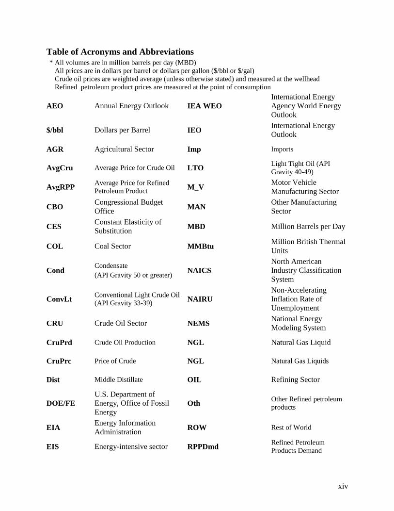
Table of Acronyms and Abbreviations * All volumes are in million barrels per day (MBD) All prices are in dollars per barrel or dollars per gallon ($/bbl or $/gal) Crude oil prices are weighted average (unless otherwise stated) and measured at the wellhead Refined petroleum product prices are measured at the point of consumption
AEO Annual Energy Outlook IEA WEO International Energy Agency World Energy Outlook
$/bbl Dollars per Barrel IEO International Energy Outlook
AGR Agricultural Sector Imp Imports
AvgCru Average Price for Crude Oil LTO Light Tight Oil (API Gravity 40-49)
AvgRPP Average Price for Refined Petroleum Product M_V Motor Vehicle
Manufacturing Sector
CBO Congressional Budget Office MAN Other Manufacturing
Sector
CES Constant Elasticity of Substitution MBD Million Barrels per Day
COL Coal Sector MMBtu Million British Thermal Units
Cond Condensate (API Gravity 50 or greater) NAICS
North American Industry Classification System
ConvLt Conventional Light Crude Oil (API Gravity 33-39) NAIRU
Non-Accelerating Inflation Rate of Unemployment
CRU Crude Oil Sector NEMS National Energy Modeling System
CruPrd Crude Oil Production NGL Natural Gas Liquid
CruPrc Price of Crude NGL Natural Gas Liquids
Dist Middle Distillate OIL Refining Sector
DOE/FE U.S. Department of Energy, Office of Fossil Energy
Oth Other Refined petroleum products
EIA Energy Information Administration ROW Rest of World
EIS Energy-intensive sector RPPDmd Refined Petroleum Products Demand

xv
ELE Electricity Sector RPPPrc Refined Petroleum Products Price
Exp Exports RUS Russia
GAS Natural Gas Sector SRV Commercial Sector
GDP Gross Domestic Product TRK Commercial trucking sector
GPL Gas Plant Liquid TRN Other Commercial Transportation Sector
GPM Global Petroleum Model U.S. United States of America
Gsl Gasoline WTI West Texas Intermediate
HCRU Heavy Crude Oil (API Gravity 22 or less)
ICRU Intermediate Crude Oil (API Gravity 23-32)

xvi
Naming Convention for Model Runs The following is the naming convention used for all model runs. All model runs are considered cases. Model runs where the ban remains in effect are referred to as baselines. Model runs where the ban is lifted in some form or way are referred to as scenarios. Lists of all the possible U.S., international, and U.S. oil export model runs are shown below.
U.S. Cases: Ref U.S. Reference Case HOGR High Oil and Gas Resource Case LOP Low Oil Price Case
International Cases:
{default} International Reference Case LOP Low Oil Price Case LowAP International Reference Case except Low Petroleum Demand in Asia-
Pacific
Ban Cases :
Ban U.S. bans all crude oil exports
NoBanCond U.S. allows exports of condensate only starting in 2015
NoBan U.S. allows exports of all crude oil types starting in 2015
NoBanDelay U.S. allows exports of all crude oil starting in 2020
OPEC Cases:
{default} OPEC competes in the market OPECFix OPEC maintains crude oil exports OPECCut OPEC cuts crude oil exports to maintain crude oil price
Baselines: Cases with Ban in-effect:
Ban_Ref U.S. and International Reference Cases with crude oil ban in-effect; OPEC competes in the market
BanLowAP_Ref U.S. Reference Case and Low Demand in Asia-Pacific Case with ban in-effect; OPEC competes in the market
Ban_HOGR U.S. High Oil and Gas Resource Case and International Reference Case with ban in-effect; OPEC competes in the market
BanLowAP_HOGR U.S. High Oil and Gas Resource Case and Low Demand in Asia-Pacific Case with ban in-effect; OPEC competes in the market
Ban_LOP U.S. and International Low Oil Price Cases with ban in-effect; OPEC competes in the market

xvii
Scenarios: Cases where ban in lifted in some way
NoBanCond_Ref U.S. Reference Case and International Reference Case with condensate export ban lifted in 2015; OPEC competes in the market
NoBan_Ref U.S. Reference Case and International Reference Case with crude oil export ban lifted in 2015; OPEC competes in the market
NoBanDelay_Ref U.S. Reference Case and International Reference Case with crude oil export ban lifted in 2020; OPEC competes in the market
NoBanOPECFix_Ref U.S. Reference Case and International Reference Case with crude oil export ban lifted in 2015; OPEC maintains crude oil exports
NoBanOPECCut_Ref U.S. Reference Case and International Reference Case with crude oil export ban lifted in 2015; OPEC cuts crude oil exports to maintain price
NoBanLowAP_Ref U.S. Reference Case and Low Demand in Asia-Pacific Case with crude oil export ban lifted in 2015; OPEC competes in the market
NoBanCond_HOGR U.S. High Oil and Gas Resource Case and International Reference Case
with condensate export ban lifted in 2015; OPEC competes in the market NoBan_HOGR U.S. High Oil and Gas Resource Case and International Reference Case
with crude oil export ban lifted in 2015; OPEC competes in the market NoBanDelay_HOGR U.S. High Oil and Gas Resource Case and International Reference Case
with crude oil export ban lifted in 2020; OPEC competes in the market NoBanOPECFix_HOGR U.S. High Oil and Gas Resource Case and International Reference Case
with crude oil export ban lifted in 2015; OPEC maintains crude oil exports
NoBanOPECCut_Ref U.S. High Oil and Gas Resource Case and International Reference Case with crude oil export ban lifted in 2015; OPEC cuts crude oil exports to maintain price
NoBanLowAP_HOGR U.S. High Oil and Gas Resource Case and Low Demand in Asia-Pacific Case with crude oil export ban lifted in 2015; OPEC competes in the market
NoBan_LOP U.S. and International Low Oil Price Cases with crude oil export ban
lifted in 2015; OPEC competes in the market

EXECUTIVE SUMMARY
1
EXECUTIVE SUMMARY
A. What NERA Was Asked to Do
U.S. petroleum markets are in the midst of a major shift in energy production. The commercialization of new exploration and production (E&P) technologies (multi-stage hydraulic fracturing, horizontal drilling, and 3D seismic) have created the opportunity to develop tight oil1 and natural gas from shale economically on a potentially very large scale. These new and potentially large sources of domestically produced crude oil and natural gas have resulted in lower natural gas prices and a lessening of U.S. dependence on imported crude oil. However, the rapid rise in production of tight oil in new locations has strained the U.S. pipeline transportation system creating temporary bottlenecks and localized depression of crude oil prices. These bottlenecks are being alleviated rapidly by new construction and reversal of pipelines,2 moving the bottleneck to the U.S. Gulf Coast where the ban on crude oil exports becomes the operative constraint.
NERA Economic Consulting was asked by the Brookings Institution to perform an analysis of the economic impacts on the U.S. economy resulting from lifting the crude oil export ban. As part of this analysis, NERA considered the following four factors which could potentially affect the impact of lifting the crude oil export ban:
1. U.S. shale oil production potential;
2. The scope and timing for lifting the ban;
3. Uncertainty in global energy markets; and
4. OPEC’s response to the U.S. lifting its ban on exports.
This report focuses on the broad and robust conclusions that can be derived from the study concerning impacts on the economy, on consumers, and on crude oil and refined petroleum product markets when crude oil exports are allowed. It also corrects errors in economic reasoning and refutes myths about trade that have appeared in controversies over energy exports.
1 Light tight crude oil is a form of light sweet crude oil contained in low permeability shale or tight sandstone. The
low permeability impedes the natural flow of crude oil into a well bore. These technology developments have greatly improved the profitability of producing crude oil from these formations.
2 Transportation bottlenecks are a result of supply expanding faster than transportation capacity to move the crude oil to market. Transportation capacity is being added to address current bottlenecks, but depending on the growth rate of production in the future, other temporary bottlenecks may occur in the future.

EXECUTIVE SUMMARY
2
B. NERA’s Approach
NERA used its Global Petroleum Model (GPM) and NewERA model to perform the analysis. GPM is a partial equilibrium model of the petroleum industry and is designed to quantify the impact of lifting the crude oil export ban on energy markets both in the U.S. and elsewhere. NewERA is a computable general equilibrium model of the U.S. economy. It determines how changes in the global energy market would ripple through the U.S. economy and affect overall economic performance as well as individual sectors and sources of income. In order to derive robust conclusions about these impacts, NERA analyzed a set of eighteen cases that considered different options or values for the four factors described above:
• U.S. crude oil production potential: reference (Ref) or high oil and gas resource (HOGR) modeled after the AEO 2014 Reference and High Oil and Gas Resource cases, respectively;
• Proposals to lift the ban: allow condensate only to be exported, lift the entire ban in 2015, or delay lifting the entire ban until 2020;
• Outlooks for global energy markets: Ref (again modeled on the AEO 2014 Reference case for the U.S. and IEO 2013 Reference case for non-North American regions), low crude oil prices, or lower demand for refined petroleum products in Asia Pacific; and
• OPEC’s response to the lifting of the ban: responds competitively like all other producers, cuts exports to maintain crude oil price, or maintains export levels and allows crude oil prices to decline.
In this executive summary, we present ranges based upon the highest and lowest results relative to each baseline rather than discussing each individual case.3
C. Key Findings
This study reaches the following conclusions about lifting the crude oil export ban:
• The U.S. economy will benefit and benefits are widespread;
• Consumers will benefit through higher real incomes and lower energy costs;
• International and domestic market conditions affect the magnitude of benefits, but under all conditions analyzed the U.S. economy gains ; and
• Benefits are greatest if the ban is lifted immediately for all types of crude oil.
3 Ranges are not presented for the low world oil price case because we found the ban has no measurable effect.

EXECUTIVE SUMMARY
3
1. Why Lifting the Crude Oil Export Ban Would Yield Positive Economic Impacts
Lifting the crude oil export ban benefits the U.S. in three ways:
• U.S. producers can sell crude oil into the global market for prices that exceed their cost of production;
• Capital that would be used by refiners to reconfigure their refineries to use additional quantities of light oils can be employed elsewhere in the economy in more profitable investments when those oils are exported; and
• Terms of trade improve for the U.S. as it reduces its net imports of crude oil and prices of imported crude oil and refined petroleum products like gasoline fall.
Lifting the export ban would remove an artificial barrier to crude oil production, thus allowing the U.S. to take full advantage of its competitive cost advantage in the production of crude oil versus producers in other parts of the world. The result would be lower crude oil prices worldwide. Lower crude oil prices translate into lower refined petroleum product prices because refineries will have on the margin lower crude oil acquisition costs and be able to operate with more flexibility in their selection of crude oil to process. Since refined petroleum products are already traded globally (unlike crude oil, the U.S. currently both imports and exports refined petroleum products) lower global prices for refined petroleum products means lower refined petroleum product prices in the U.S.
a. Additional Production of Crude Oil
The immediate effect of lifting the ban on exports would be to increase investment in oil exploration and development, and thereby increase domestic crude oil production.
Figure 1 shows that the level of increased production depends on the abundance and longevity of the resource. In the Ref case, the increase in production would tail off over time mirroring the EIA Reference case in which crude oil peaks then declines. In the HOGR scenario, production would increase by 2.1 MBD in 2015 and by a larger increment of 4.3 MBD in 2035 as the ability to produce from tight resources improves over time.

EXECUTIVE SUMMARY
4
Figure 1: Incremental Crude Oil Production Resulting from the Complete Lifting of the Crude Oil Export Ban in 2015 (Ref and HOGR Baselines: MBD)
Lifting of the crude oil export ban would remove a regulatory barrier that has artificially suppressed the price of both light tight crude oil and condensate and as a result minimized their production. With the crude oil export ban lifted all crude oil produced in the U.S. would compete freely in the global market and receive value commensurate with the global price of crude oil. In the U.S., lifting the crude oil export ban would reduce the price spreads between light crude oils (i.e., light tight crude oil and condensate) and intermediate crude oil. The higher price for light crude oils means a greater number of economic prospects and higher levels of crude oil production.
b. Lower Net Imports of Crude Oil
Production of light crude oils is suppressed by the export ban because a large price spread between light oils and intermediate crudes is needed to incentivize refiners to modify their operations to increase their blending of the light crude oils with other crude oils and/or invest in reconfiguring domestic refineries to substitute domestic light crude oils for imported heavier crude oils. When the ban is lifted and the price spread collapses, most of the increased production of light crude oils will be exported. Figure 2 illustrates this, showing that in the HOGR case, the increases in U.S. crude oil exports are offset to a small degree by an increase in imports, so that the change in net imports is slightly less than the change in exports.
0.0
1.0
2.0
3.0
4.0
5.0
2015 2020 2025 2030 2035
MB
D
REF HOGR
EXECUTIVE SUMMARY
5
Figure 2: Change in Exports, Imports, and Net Imports Resulting from the Complete Lifting of the Crude Oil Export Ban in 2015 (Ref and HOGR Baselines: MBD)
Even with the lifting of the crude oil export ban, the U.S. will remain a net importer of crude oil. The U.S. currently imports 7.7 MBD of crude oil and exports about 0.3 MBD of crude oil; the latter almost entirely to Canada. Lifting of the ban will have a substantial impact on the level of crude oil exports (see Figure 2). The increase in exports in the HOGR case would become larger over time, rising from 2.1 MBD in 2015 5.8 MBD in 2035. The partially offsetting increase in imports would grow much more slowly, so that the amount that net imports would fall increases over time.
In the Ref case, increases in crude oil exports are also partially offset by an increase in imports in 2015. This increase in imports stays constant over time; whereas the increase in crude oil exports tails off, so that by 2035 the increase in imports is equal to the increase in exports. Thus by 2035 the benefit of removing the export ban takes the form of greater efficiency in the refining system due to the increased ability of U.S. refineries to utilize the types of crude oil for which their design is optimized.
-6
-5
-4
-3
-2
-1
0
1
2
3
4
5
6
2015 2020 2025 2030 2035
MB
D
Change in ExportsChange in ImportsChange in Net Imports
Ref
2015 2020 2025 2030 2035
Change in ExportsChange in ImportsChange in Net Imports
HOGR

EXECUTIVE SUMMARY
6
c. World Crude Oil Prices Decline
The additional supply of U.S. crude oil in the world market will lead to a reduction in world oil prices; unless OPEC cuts back exports sufficiently to fully offset the increase in U.S. exports.
Figure 3: Change in Average Rest of World Crude Oil Price Resulting from the Complete Lifting of the Crude Oil Export Ban in 2015 (Ref and HOGR Baselines: $/bbl)
The ban on crude oil exports now in place has caused world crude oil prices to be inflated. Exports of U.S. crude oil would bring down crude oil prices outside the U.S. until world and domestic crude oil prices reach a common equilibrium. Increased U.S. production made possible by exports would increase worldwide supply and therefore decrease global crude oil prices. The degree to which crude oil prices would be affected depends on the outlook for the resource base of U.S. light crude oils. Figure 3 shows the projected decline in crude oil prices outside the U.S. for both the Ref and the HOGR scenarios. In the Ref case the largest impact is on world oil prices in 2015. It declines over the years as the production of light crude oils falls off in the U.S. In the HOGR case, the reduction in world oil prices ranges between $5 and $7 per barrel.
-$8
-$7
-$6
-$5
-$4
-$3
-$2
-$1
$02015 2020 2025 2030 2035
$/bb
l
REF HOGR

EXECUTIVE SUMMARY
7
Figure 4: Change in the U.S. Gasoline Price Resulting from the Complete Lifting of the Ban in 2015 (Ref and HOGR Baselines: $/gal)
Motor gasoline prices at the refinery move directly with changes in global crude oil prices. Since lifting the crude oil export ban would put more crude oil supply onto the world market resulting in lower crude oil prices, gasoline prices would also fall. Since gasoline is imported freely into the U.S. at global prices, the cost of the marginal U.S. supplier of gasoline will decline as will the price of gasoline at the pump. Figure 4 illustrates that the impact on gasoline prices will be a function of the abundance and longevity of the shale crude oil. In the Ref case where the light crude oils boom is more of a short term phenomena, any decrease in gasoline price will be short term; $0.08/gallon in the near term to almost zero in the long term. However, should the light crude oil resource prove to be abundant then the impact on gasoline prices will be between $0.09/gallon and $0.12/gallon depending on the year and continue throughout the forecast period.
d. Refinery Gross Margin would remain within the Historical Range
Since imported refined petroleum products, in particular gasoline, set the price of those products in the U.S., increases in U.S. crude oil prices will not be felt by U.S. consumers, but they will erode the margins of some refiners with access to currently lower cost light crude oils. Individual refiners will experience this reduction in gross margin to different degrees, and on average the decline in gross margin will still leave them with gross margin near the average for the past 14 years.
-$0.14
-$0.12
-$0.10
-$0.08
-$0.06
-$0.04
-$0.02
$0.002015 2020 2025 2030 2035
$/ga
l
REF HOGR

EXECUTIVE SUMMARY
8
Figure 5: Historical U.S. Refinery Gross Margin and Forecasted U.S. Refinery Gross Margins under Different Assumptions about the U.S. Crude Oil Export Ban and Availability of U.S. Crude Oil Resources (Ref and HOGR Baselines: $/bbl)4
2. The U.S. Economy Will Benefit from Lifting the Crude Oil Export Ban
The economy overall would improve with the lifting of the crude oil export ban. Figure 6 displays the range of the changes in U.S. welfare and GDP from modifying the U.S. crude oil export ban. Welfare – the most comprehensive measure of the improvement in national economic wellbeing –improves by about one-tenth of one percent in Ref and by one-tenth to over four-tenths of a percent in HOGR.
4 Historical portion calculated using EIA data.
$0
$5
$10
$15
$20
$25
$30R
efin
ery
Gro
ss M
argi
ns ($
/bbl
)
Historical Ref Ban Case Ref No Ban CaseHOGR Ban Case HOGR No Ban Case
Historical Future

EXECUTIVE SUMMARY
9
Figure 6: Range of Change in U.S. Welfare Resulting from the Partial or Complete Lifting of the Crude Oil Export Ban (Ref and HOGR Baselines: %)
Even though the improvement in welfare is less than 1 percent, it accumulates over many years. The benefit of this accumulation can be seen by looking at the change in overall economic activity as measured by GDP. With growing GDP between now and 2039, the net present value of the gain in GDP from lifting the ban is between $200 billion and $1.8 trillion, based on the resource outlook and the type of policy lifting the ban (see Figure 7).
0.0
0.1
0.2
0.3
0.4
0.5
Ref HOGR
% C
hang
e in
Wel
fare
fro
m b
asel
ine

EXECUTIVE SUMMARY
10
Figure 7: Range of Change in Net Present Value of GDP Resulting from the Partial or Complete Lifting of the Crude Oil Export Ban (Ref and HOGR Baselines: Billion $)5
The low end of the range occurs if the export ban were lifted only for condensates or if the lifting of the ban were delayed until 2020. Immediate lifting of the ban in 2015 would generate the greatest benefits to the overall economy.
Overall, we observe that:
• All scenarios have positive changes in welfare and GDP for all ways of modifying the ban.
• All restrictions on crude oil exports are harmful to the economy. Partial restrictions are less harmful but partial or delayed modification of the ban fails to completely remove the distortion.
• Benefits increase with more trade. The low end of the range occurs for the case in which the U.S. lifts the ban only on exporting condensates. The high end of the range occurs when the U.S. lifts the ban in 2015 for all types of crude oil. Delaying the lifting of the ban also puts benefits at the bottom of the range for Ref, somewhat higher for HOGR because tight oil production peaks in 2020 in the Ref case.
5 Unless otherwise noted, all dollar figures ($) are stated in terms of 2013 dollars.
0
200
400
600
800
1000
1200
1400
1600
1800
2000
Ref HOGR
Ran
ge o
f Cha
nge
in G
DP
(Bill
ion
$)

EXECUTIVE SUMMARY
11
• The potential gains from removing the export ban increase as the resource base increases. If the oil and gas resource base is larger, an export ban will be more restrictive as larger resources create greater potential for production of light oils above domestic refinery capabilities.
• Even if OPEC cuts its output to offset the effect of U.S. exports on world oil prices, the study finds removing the ban on exports would still provide both economic benefits and energy security benefits. If OPEC cut production in response to U.S. crude oil exports, a significantly smaller fraction of the world’s oil supply would be produced in regions that are vulnerable to supply disruptions.
3. Consumers Would Benefit from Lifting the Crude Oil Export Ban
a. Household Earnings and Payments
The benefit to consumers appears both in what they pay for goods and services and what they receive for their labor.
Figure 8: Range of Change in Real Wages in 2015 and 2035 Resulting from the Partial or Complete Lifting of the Crude Oil Export Ban (Ref and HOGR Baselines: %)
0.0
0.1
0.2
0.3
0.4
0.5
0.6
0.7
2015 2035 2015 2035
% C
hang
e in
Rea
l Wag
e
Ref HOGR

EXECUTIVE SUMMARY
12
Figure 9: Range of Change in U.S. Gasoline Prices in 2015 and 2035 Resulting from the Partial or Complete Lifting of the Crude Oil Export Ban (Ref and HOGR Baselines: $/gal)
In all scenarios, lifting the ban leads to increased wage rates (Figure 8) and lower gasoline prices (Figure 9). Therefore, lifting the ban not only puts more money in consumers’ pockets, but also gives them more purchasing power for every dollar earned because their energy costs decline. Thus a policy to lift the ban on crude oil distributes benefits widely throughout the economy and benefits all segments, no matter what their source of income.
Benefits correlate directly with the level of crude oil that can be cost-effectively exported. Therefore gains are greater under the HOGR scenarios because of greater crude oil supplies and when the ban is fully removed as quickly as possible because all types of crude oil are available for export.
b. Near-term Benefits – Hastening the Recovery to Full Employment
Unemployment in the U.S. economy is projected to persist until 2018, but from then on the Congressional Budget Office and other leading forecasters expect the U.S. to return to effective full employment, with the unemployment rate down to a level consistent with stable prices. Therefore, we only estimate reductions in unemployment in the first period of analysis, 2015 – 2020. Investment in oil production and infrastructure and increased earnings from exports will boost the demand for labor throughout the economy, and if the ban is lifted in 2015 the resulting acceleration in economic growth will take an average of 230,000 to 380,000 workers off the
-$0.20
-$0.15
-$0.10
-$0.05
$0.00
2015 2035 2015 2035
Cha
nge
in G
asol
ine
Pric
es ($
/gal
)
Ref HOGR

EXECUTIVE SUMMARY
13
unemployment rolls in the next 5 years, with the largest improvement in the years 2015 and 2016. These employment benefits largely disappear if lifting the ban is delayed until 2020 because by then the economy will have returned to full employment.
Figure 10: Average Annual Reduction in Unemployment (2015 – 2020) Resulting from the Lifting of the Crude Oil Export Ban in 2015 versus 2020 (Ref and HOGR Baselines)
4. How Market Conditions Impact Economic Benefits
The economic impacts on the U.S. economy from lifting the crude oil ban depend critically on the amount of crude oil that the U.S. can export. This amount depends on both domestic factors, as discussed above, and international factors, which this section addresses. There are a number of international factors that could affect the level of U.S. exports. Three of the most important are world demand for refined petroleum products, OPEC’s response to changes in exports from other countries, and the prevailing international crude oil price.
Since increased exports clearly lead to increased benefits for the U.S., the key question for the U.S. is the economic impacts of lifting the crude oil export ban if international demand falls thus reducing demand for U.S. exports. To assess this case, we analyzed scenarios which included a forecast of lower demand for refined petroleum products from the Asia Pacific region. As for the consequences of OPEC’s response to the U.S. becoming an exporter of crude oil, we considered three potential responses by OPEC to the lifting of the ban. Finally, we analyze the effect of the EIA’s AEO 2014 Low Oil Price (LOP) scenario on the U.S. oil market to examine the consequences of an oil price collapse on production and exports of light tight crude oil.
0
50,000
100,000
150,000
200,000
250,000
300,000
350,000
400,000
Ref HOGR
Red
uctio
n in
Une
mpl
oym
ent
NoBan NoBanDelay

EXECUTIVE SUMMARY
14
a. Actions by OPEC would either increase the Economic Benefits to the U.S. or Improve Energy Security for the U.S.
In addition to the scenario where OPEC acts as another competitor in the market, we posited two alternative responses by OPEC, that bracket the assumption of competitive behavior made in other cases.
• Maintain its export levels at the levels projected for the scenario with an export ban in place; and
• Reduce its exports in an attempt to maintain crude oil prices at a level they would reach with the U.S. export ban in place.
Figure 11: Change in Net Present Value of U.S. GDP Resulting from a Complete Lifting of the Ban in 2015 under Different Assumptions about OPEC’s Actions (Ref and HOGR Baselines: Billion $)
Our analysis found that OPEC’s actions could either further enhance the economic benefits of trade to the U.S. or a measurable drop in economic benefits, but in the latter case would lead to fewer crude supplies from regions that are vulnerable to supply disruptions. Should OPEC decide to maintain its export volumes after the crude oil ban is lifted all other suppliers will experience some crowding out. For the U.S. that means lower world crude oil price resulting in a small increase in net imports of crude oil relative to the case where OPEC acts as another competitor in the market and accepts some lower level of exports. The resulting change in the economic benefits of lifting the ban would be negligible.
$0
$200
$400
$600
$800
$1,000
$1,200
$1,400
$1,600
$1,800
$2,000
Ref HOGR
Bill
ion
$
NoBan NoBanOPECFix NoBanOPECCut

EXECUTIVE SUMMARY
15
Should OPEC decide to cut exports to maintain crude oil prices, the component of U.S. economic benefits attributable to lower prices for imported oil would disappear, but oil exports would be sold in larger quantities at a higher price. Figure 11 reveals that the benefits of lower world oil prices that would disappear if OPEC cuts exports account for about half of the net economic benefits to the U.S. in the Ref scenario and about one third in the HOGR scenario.
The impact of U.S. crude oil exports on OPEC sales and revenues in the Ref case would likely be too small and transitory to provoke any kind of OPEC response. The HOGR case would make the U.S. a major new entrant into the global market and could have an impact on OPEC large enough to bring about a coordinated response.
However, global energy security would improve substantially if OPEC were to cut exports to maintain world crude oil prices, Figure 11 depicts the percentage reduction in OPEC exports for each case. It shows for example that if OPEC cuts exports in 2015 sufficiently to offset U.S. exports, 12% to 18% less crude oil would be exported from regions vulnerable to supply disruptions.
Figure 12: Change in OPEC’s Exports of Crude Oil Resulting from a Complete Lifting the Ban in 2015 under Different Assumptions about OPEC’s Actions (Ref and HOGR Baselines: %)
b. Lower than Expected Petroleum Demand in Asia Pacific Would Not Significantly Diminish Economic Benefits to the U.S.
If for reasons unrelated to the lifting of the crude oil export ban, the Asia-Pacific region’s demand for refined petroleum products were to be lower than expected, the benefits of lifting the crude oil export ban would remain essentially the same (Figure 13).
Two simultaneous offsetting factors account for the similarity of benefits:
1. World petroleum production and consumption are smaller in the scenario of lower Asia Pacific demand than in the other NoBan scenarios. As a result, the incremental U.S.
-25%
-15%
-5%
2015 2020 2025 2030 2035
Perc
ent C
hang
e in
OPE
C E
xpor
ts
NoBanOPECCut NoBanOPECFixRef
2015 2020 2025 2030 2035
NoBanOPECCut NoBanOPECFix
HOGR

EXECUTIVE SUMMARY
16
production becomes a larger percentage of the total world-wide production and thus leads to a larger drop in world oil prices;
2. U.S. crude oil exports are smaller because of the lower world price resulting from lower Asia Pacific demand. As a result the economic gains from derived from exports when the ban is lifted are limited.
Figure 13: Change in Net Present Value of U.S. GDP Resulting from a Complete Lifting of the Ban in 2015 (Ref and Ref with LowAP Baselines: Billion $)
c. Low Global Crude Oil Prices Would Make the Crude Oil Export Ban Harmless
The AEO 2014 Low Oil Price scenario forecasts the international crude oil price to begin at $70/bbl in 2015 and rise to less than $75/bbl by 2035. This current production costs of light tight crude oil and condensates are close to this value so international crude oil prices in this range reduce and even eliminate the crude oil price spread6 that stimulates more U.S. production. A spread of only a few dollars in crude oil price between U.S. light tight crude oil and intermediate crude oil and between U.S. light tight crude oil and international light tight crude oil with the crude oil export ban in place means if the crude oil export ban is lifted there would be little incentive to produce more light tight crude oil because the market could not bear the higher cost
6 The difference in price between intermediate crude oil (API gravity 22-32 degrees) and light tight crude oil (API
gravity 40-49 degrees) or condensate (API gravity 49+ degrees).
$0
$200
$400
$600
$800
$1,000
$1,200
$1,400
$1,600
$1,800
$2,000
Ref HOGR
Bill
ion
$
NoBan NoBanLowAP

EXECUTIVE SUMMARY
17
of production. As a result, when the ban is lifted, the minimal additional production and exports of light tight crude oil and condensate is less than 0.2 MBD.
5. Lifting the Ban Immediately on all Types of Crude Oil Would Yield the Greatest Economic Benefits
A number of alternative proposals have been offered to modify the current ban on crude oil exports. They range from limiting the crude oils that would qualify for export or delaying the lifting of the ban to full and immediate elimination of the ban.Figure 14 reports the percentage change in welfare (or economic wellbeing) over the model horizon from three different changes to the crude oil export ban: Immediate and complete removal in 2015 (NoBan), complete removal in 2020 (NoBanDelay), and immediate removal of the ban for condensate (NoBanCond). The figure reports these results for the Ref and HOGR cases.
Figure 14: Change in Net Present Value of Welfare Resulting from a Complete Lifting of the Ban in 2015 compared to a Complete Lifting of the Ban in 2020 and Lifting of the Ban on only Condensates (Ref and HOGR Baselines: Billion $)
Delaying the lifting of the crude oil ban by five years, until 2020, would sacrifice the economic benefits associated with free trade in oil during the five year delay. Since these are the years of peak production in the Ref scenarios, about half of the benefits of lifting the ban disappear. With sustained production in the HOGR case, the loss of benefits in dollar value is much greater but the larger dollar loss is a smaller percentage of the total gain. In the Ref scenario delaying or allowing only condensate exports results in about a 60% reduction in gains compared to a
0
200
400
600
800
1,000
1,200
1,400
1,600
Ref HOGR
Bill
ion
$
NoBan NoBanDelay NoBanCond
EXECUTIVE SUMMARY
18
complete and immediate removal of the ban. In the HOGR scenario, delaying the removal of the ban causes a 30% reduction in welfare; but removing the ban on only condensates, yields almost 75% fewer benefits than a complete and immediate removal.
Lifting the ban for condensate exports alone has proportionately smaller impacts compared to lifting the ban for all types of crude oil. Condensates, defined in our study as crude oil with an API gravity greater than 49, and LTO, defined in our study as crude oil with an API gravity between 40 and 49, are the two primary crude oils with potential for export if the crude oil ban is lifted for all crude types, yet condensates only make up 18% to 24% of this export potential in any given year. Therefore, the benefits of lifting the ban on only condensate are considerably smaller (Figure 14).
Introduction
19
I. INTRODUCTION
The Brookings Institution provided funding to NERA Economic Consulting to perform an analysis of the impacts on the U.S. economy resulting from lifting the crude oil export ban. This report discusses the motivation for this analysis, how the analysis was performed, and the results and insights from this analysis. NERA's analysis is intended to complement and support the work of the Brookings Crude Oil Task Force, but it has been performed independently and is being published simultaneously but separately.
U.S. petroleum markets are in the midst of a major shift in direction. The commercialization of new exploration and production (E&P) technologies (multi-stage hydraulic fracturing, horizontal drilling, and 3D seismic) have created the opportunity to economically develop tight crude oil7 and natural gas from shale on a potentially very large scale. These new potentially large sources of domestically produced crude oil and natural gas have reversed the U.S.’s trend in crude oil and natural gas production, resulting in lower natural gas prices and a lessening of U.S. dependence upon imported crude oil. However, the rapid rise in production of light tight crude oil in new locations has strained the U.S. pipeline transportation system creating temporary bottlenecks and localized depression of crude oil prices. These bottlenecks are being rapidly alleviated through new construction and reversal of pipelines8, moving the bottleneck to the U.S. Gulf Coast where the ban on crude oil exports becomes the operative constraint. However, as production continues to increase there is the potential for new temporary transportation bottlenecks to reemerge.
Over the past several decades the U.S. refining system added capacity for processing9 heavy, crude oils because of their availability and the price discount at which such crude oils have historically been sold relative to lighter crude oils. Shale formations yield very light crude oils.10 However, refineries designed to process heavy, sour crude oils lack capacity in their downstream units to handle the higher percentages of light fractions contained in the lighter oils (light tight crude oil and condensate). Thus, it is becoming difficult to find U.S. refineries with available capacity that is designed to process those crude oils efficiently.
7 Light tight crude oil is a form of light sweet crude oil contained in low permeability shale or tight sandstone. The
low permeability impedes the natural flow of crude oil into a well bore. These technology developments have greatly improved the profitability of producing crude oil from these formations.
8 Transportation bottlenecks are a result of supply expanding faster than transportation capacity to move the crude oil to market. Although transportation capacity is being added to address current bottlenecks and depending upon the growth rate of production in the future, other bottlenecks may arise.
9 Refiners in coking units that process relatively low cost heavy sour crude oils into more of the lighter and most profitable products gasoline and diesel fuel.
10 The crude oils produced from shales often have API gravities greater than 40 degrees. In this report we refer to crude oils from shale formations with API gravities from 40 to 49 as light tight crude oil. Crude oils with API gravity greater than 49 are referred to as condensate.
Introduction
20
Finally, under legislation passed in 1975 and 197911 the U.S. prohibits exports of crude oil,12 with a few exceptions,13 thus confining the market for light tight crude oil and condensate to refineries within the United States that are not necessarily designed to process it in the volumes that could be produced with current technology. The U.S. restriction on crude oil trade contrasts with other major oil producing countries, all of which allow exports of crude oil. As a consequence, the prices of U.S. light tight crude oil and condensate have become depressed relative to comparable crude oils sold on the world market. This has limited U.S. crude oil production because lower crude oil prices mean less of the crude oil resource in the ground is economic to produce. Conversely, it has increased the profitability of some U.S. refiners, particularly those that can both access and are configured to process the light tight crude oil produced from shale. Since refined products are imported and exported freely, their prices are set by the global market, so that the ban on crude oil exports provides no benefit to consumers.
This next section describes the issues that relate to the export of crude oil from the U.S. and the scope of NERA’s analysis, including the impacts on the energy industry and the overall U.S. economy.
A. Problem Statement
1. What Would Be the Impacts on the Domestic and International Energy Markets Resulting from the U.S. Lifting its Crude Oil Export Ban?
Permitting crude oil exports would allow crude oil produced in the U.S. to compete globally with crude oil produced in other regions of the world, which would likely result in a greater supply of crude oil worldwide. This greater supply would tend to lower crude oil prices outside the U.S., which in turn would lead to lower refined petroleum product prices in world markets. Since there is clear evidence that U.S. gasoline prices are more closely tied to world gasoline prices than to U.S. crude oil prices, lower gasoline prices in the U.S. would occur.14
For the United States the impacts could be felt in all steps of the petroleum value chain. Crude oil production would increase as crude oil prices increase. There would likely be a greater need
11 Energy Policy and Conservation Act (EPCA) of 1975 and the Export Administration Act (EAA) of 1979. At the
time these controls were enacted, some oil produced in the U.S. was subject to price controls that held its price well below world market levels, and maintenance of the price control system required an export ban to prevent all of the price controlled oil from being sold overseas. When all oil price controls were lifted in 1981, this need disappeared.
12 Crude oil is unique with regards to exports. Refined petroleum product exports occur without limitation, natural gas exports are being authorized in an orderly way, and coal exports have gone on for many years.
13 Like for like exchanges, exports of crude oil imported from another country and not intermixed with U.S. crude oils, and exports of crude oil that cannot be sold in the U.S. are major exceptions, each of which is dealt with on a case-by-case basis by the Department of Commerce.
14 Brown, S., Mason, C, Krupnick A., Mares J. Crude Behavior: How Lifting the Export Ban Reduced Gasoline Prices in the United States. Resources for the Future. February 2014.

Introduction
21
for transportation infrastructure to handle the movement of crude oil to coastal locations for export. Lower refined petroleum product prices would lead to higher demand for gasoline and other refined petroleum products. With the removal of the export ban, refineries could choose between importing an optimum mix of crude oils based upon their current configuration and investing to change their configuration to optimally process light oil. Having this added flexibility in the market would lower overall refining costs and hence lower prices for refined petroleum products.
To quantify impacts on the U.S. oil market, this study used a global crude oil and petroleum markets model to analyze the following metrics:
• U.S. gasoline, distillate, and other refined petroleum product prices at a national level;
• Production of crude oil and refined petroleum products;
• Import and export levels for crude oil and refined petroleum products; and
• U. S. and world crude oil prices by type of crude oil.
2. What would be the Economic Impacts on the U.S. Economy resulting from Crude Oil Exports?
Lifting the ban on U.S. crude oil exports will clearly affect U.S. energy markets. These effects will ripple through the U.S. economy. To account for the economic impacts on the U.S. from the lifting of the ban, the study used a macroeconomic model of the U.S. economy to measure the following key impacts:
• Net economic benefits in terms of standard metrics of welfare and GDP on a national basis;
• Impacts on sources of income, employment, and industry output on a national basis; and
• Effects on aggregate employment during the recovery from the recession.
B. Scope of this Study
The analysis concept and methodology adopted for this NERA study is similar to recently published NERA LNG studies15. The study focuses on the benefits of trade; and it develops and lays out broad and robust conclusions about impacts on the economy, on consumers, and on crude oil and refined petroleum product markets from allowing exports of crude oil. It also
15 Baron R, Bernstein P, Montgomery D, Tuladhar S, Xiong S, Yuan M. Macroeconomic Impacts of LNG Exports
from the United States. NERA Economic Consulting, July 16, 2012.
Introduction
22
corrects errors in economic reasoning and refutes myths that have appeared in the controversy over lifting the ban on crude oil exports.
C. Organization of this Report
This report begins by describing the scope of the report and the methodology followed by NERA more fully. Section II describes the models developed and used to perform this analysis and includes the key assumptions underpinning the results. Section III describes the various scenarios analyzed along with key assumptions. Section IV presents the results from NERA’s Global Petroleum Model (GPM). In Section V, the macroeconomic impacts on the U.S. economy are discussed. The Appendices A, B, and C contain, respectively, extensive details on the input data, description of the models used, and the results from each scenario that was analyzed. Appendices D and E provide a detailed outline of the scenarios run and examples of refinery investment projects.

Description of Global Petroleum Markets and NERA’s Analytical Models
23
II. DESCRIPTION OF GLOBAL PETROLEUM MARKETS AND NERA’S ANALYTICAL MODELS
A. Global Petroleum Markets
Crude oil and refined petroleum products are traded on a global basis. The value chain proceeds from crude oil exploration and production through crude oil transportation, refining, distribution to retail sales and consumption of refined petroleum products.
The system by which the oil industry produces crude oil, converts the crude oil to refined petroleum products, and then transports these products to end-users such as local retail stations for sale to the public is complex. Crude oil is produced in oil fields located around the world and is transported in bulk, either through pipelines, rail, or by water to refineries where it is processed into a variety of refined petroleum products. In the United States, many of these refineries are located in the Gulf Coast region. Along the East Coast, refineries are concentrated in the mid-Atlantic region and on the West Coast in Los Angeles and San Francisco Bay areas; the rest are found in other strategic locations around the United States. At the refinery, crude oil is chemically processed and its components physically separated to produce a variety of refined petroleum products, which include motor gasoline, middle distillate fuels such as diesel fuel, and other refined petroleum products such as chemical plant feedstocks and heavy fuel oil.
Refineries are generally classified by their degree of complexity: that is the extent of oil processing downstream of the distillation column. In general, refineries can be divided into three categories:
1. Hydro skimmers which are the least complex and have only a minimum amount of downstream processing. These refineries generally process relatively light crude oil.
2. Cracking refineries are more complex and contain sophisticated upgrading units to convert heavy refined oil into lighter oil, such as gasoline and middles distillates. These refineries can process a wide variety of crude oils depending upon their specific configuration.
3. Coking refineries are the most complex and contain the same units as a cracking refinery and in addition have upgrading units termed "cokers" for additional upgrading of heavy refined oil. These refineries are designed to process heavy crude oil.
Regardless of the refinery where it is produced, each type of motor gasoline and diesel fuel must conform to the same set of product specifications for that type of motor fuel. The same requirement applies to the other refined petroleum products.
Once produced, these fuels are delivered to major market areas by several modes of transportation. The route a refined petroleum product takes from the refinery to the end-user of the product depends on the type of fuel and type of end-user. The two principal means of

Description of Global Petroleum Markets and NERA’s Analytical Models
24
transporting large volumes of refined petroleum products are dedicated refined petroleum product pipelines and waterway shipment by tanker or barge. If available, these are the lowest cost forms of transportation. A network of refined petroleum product pipelines exists across the United States, moving these products from refineries to major markets. The refined petroleum products move along pipelines in batches, which are separated volumes of a particular type of refined petroleum product. In coastal regions, either barges or tankers transport refined petroleum products on the water. Coastal shipments by tanker between U.S. ports are limited, because the Jones Act, which requires use of American built, flagged and crewed ships greatly increases their cost compared to rates for international shipments.
Refined petroleum products consumed by residential and commercial customers are generally offloaded from a pipeline or ship and then stored at facilities called terminals. Tanker trucks are loaded at these terminals to distribute motor gasoline and gasoline to local retail stations for sale to the public.
Large industrial customers, especially customers that use the refined petroleum products as feedstocks in their operations (e.g., petrochemical plants), receive their shipments more directly. Their products can be sometimes offloaded directly at their facility from a pipeline or barge, so that their purchases avoid going through a terminal and a local distribution network.
B. NERA’s Global Petroleum Model
The GPM is a partial-equilibrium model designed to estimate the amount of crude oil production, refining, refined petroleum product consumption, and trade by major crude oil producing and refined petroleum product consuming regions. The model is global but has particular focus on the North American market so as to better assess the impact of the U.S.’s existing crude oil export ban. The model simulates a market equilibrium by maximizing the sum of consumers’ and producers’ surplus less transportation and refining costs, subject to mass balancing constraints and refining and transportation capacity constraints.
The model divides the world into the following 14 regions: the five U.S. PADDs, Alaska, Western and Eastern Canada, Africa, Asia Pacific, Europe, Latin America, Middle East, and Russia. These regions are largely adapted from the EIA IEO regional definitions16, with some modifications to address the crude oil and/or oil-intensive regions. The model’s international refined petroleum product consumption and crude oil production projections for these regions are based upon the EIA’s AEO 2014 and IEO 2013 cases.
16 EIA IEO 2013: http://www.eia.gov/forecasts/ieo/regional_definitions.cfm
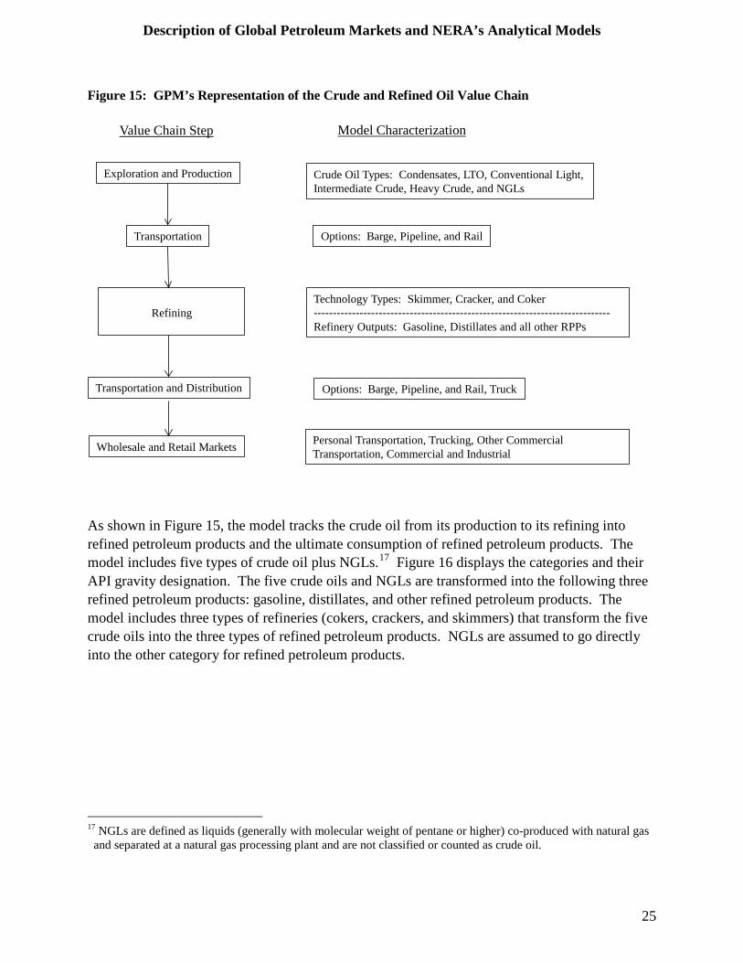
Description of Global Petroleum Markets and NERA’s Analytical Models
25
Figure 15: GPM’s Representation of the Crude and Refined Oil Value Chain
As shown in Figure 15, the model tracks the crude oil from its production to its refining into refined petroleum products and the ultimate consumption of refined petroleum products. The model includes five types of crude oil plus NGLs.17 Figure 16 displays the categories and their API gravity designation. The five crude oils and NGLs are transformed into the following three refined petroleum products: gasoline, distillates, and other refined petroleum products. The model includes three types of refineries (cokers, crackers, and skimmers) that transform the five crude oils into the three types of refined petroleum products. NGLs are assumed to go directly into the other category for refined petroleum products.
17 NGLs are defined as liquids (generally with molecular weight of pentane or higher) co-produced with natural gas
and separated at a natural gas processing plant and are not classified or counted as crude oil.
Value Chain Step Model Characterization
Exploration and Production
Refining
Wholesale and Retail Markets
Transportation
Crude Oil Types: Condensates, LTO, Conventional Light,Intermediate Crude, Heavy Crude, and NGLs
Technology Types: Skimmer, Cracker, and Coker-----------------------------------------------------------------------------Refinery Outputs: Gasoline, Distillates and all other RPPs
Personal Transportation, Trucking, Other Commercial Transportation, Commercial and Industrial
Options: Barge, Pipeline, and Rail
Transportation and Distribution Options: Barge, Pipeline, and Rail, Truck

Description of Global Petroleum Markets and NERA’s Analytical Models
26
Figure 16: API Gravities of Crude Oil Types Considered in this Report
Crude Type Abbreviation API Gravity Heavy Crude Oil HCRU 22 or less
Intermediate Crude Oil ICRU 23-32 Conventional Light Crude Oil ConvLT 33-39
Light Tight Crude Oil LTO 40-49 Condensates18 Cond 50 or greater
The supply of NGLs and all types of crude oil except U.S. condensate and light tight crude oil is represented by a constant elasticity of substitution production function. Therefore, the supply curves for each of the above mentioned fuels assume that for a given percentage change in the fuel’s price, the percentage change in its production will be the same regardless of the starting price and supply. The supply curve’s elasticity dictates how the production of fuel changes when the price of the fuel changes. The elasticity of supply is assumed to increase over time reflecting the fact that exploration and production can be more responsive in the long-run than the short-run. The elasticity of supply is assumed to be invariant across regions and fuels.
The supply curves for U.S. condensate and light tight crude oil are piecewise linear functions. The first line segment for condensate or light tight crude oil starts at the point of no supply (or zero quantity) and the choke price. The choke price represents the price below which no fuel will be produced. Based upon industry feedback, for U.S. condensates, the choke point is set at $40/bbl and the choke price for light tight crude oil is $55/bbl. The supply curves then include the reference price and quantity which match the EIA’s AEO 2014 Reference or High Oil and Gas Resource values depending on the case modeled. For the curve that extends to the right of the EIA’s data point the piecewise linear function approximates a CES function with the same elasticity as assumed for all other types of crude oil.
1. Crude Oil Transportation:
Once produced, crude oil and NGLs can be transported by up to three modes depending on location. In North America, these commodities can be moved via rail, ship, or pipeline. Outside of North America, these commodities can be transported to other regions via pipeline (where feasible) or ship. The five types of crude oil are transported to a refinery where they are
18 Questions about the definition of "condensate" have become much more complex since a widely reported
authorization by the Department of Commerce, granted to two companies, to classify "condensate" produced in particular way by separation from other crude oil components as "processed" and therefore not subject to the crude oil export ban. There is no way to tell at this point, since the Department of Commerce made these rulings in private letters and announced no general policy, what fraction of the condensates included in the category reported by EIA would become "processed" fuels and no longer subject to the export ban. Therefore, for this report NERA has continued to follow EIA's definitions and data on condensate production and trade as of July 2014.

Description of Global Petroleum Markets and NERA’s Analytical Models
27
processed into three types of refined petroleum products. NGLs feed directly into the pool of other refined petroleum products so they are effectively transported directly to final consumers.
2. Refining:
The model includes three types of refineries to process crude oil: hydroskimmer, cracker, and coker. These refineries differ in their processing yields, processing cost, and capacity. For GPM, the refinery converts crude oil into refined petroleum products in fixed proportions. The refinery yields specify these proportions. The model allows refineries to deviate from their initial yields by five percentage points. The processing yields at a refinery also vary by type of crude oil as well as type of refinery. Hydroskimmers are the least complex refiners and as such have the lowest yields for gasoline and middle distillates; whereas cokers are the most complex and thus have the highest yields for gasoline and middle distillates. The cracker yields fall between the hydroskimmers and cokers. Refining costs increase with refiner complexity and API gravity of the crude oil being refined. Therefore, the hydroskimmer has the lowest processing costs, and the cokers have the highest. Appendix A reports the refining capacity by type of refiner over time for all regions.
3. Refined Petroleum Product Transportation:
From the refinery, GPM transports the refined petroleum products to end users. The refined petroleum products can be transported via three modes in North America -- rail, ship, and pipeline – while to and from and between regions outside of North America; refined petroleum products can be moved by ship or pipeline.
4. Consumption:
Each model region demands each of the types of refined petroleum products: gasoline, middle distillate, and other refined petroleum products. Each region’s demand is specified by its constant elasticity of substitution (CES) demand curve. The benchmark demand and price for each product is based on the EIA’s forecasts (IEO 2013 and AEO 2014) demand for refined petroleum products. The demand curve elasticity varies over time becoming more elastic in the long-run. The elasticity of demand however is assumed to be the same in each region and for each refined petroleum product.
As with the supply curves, the demand curve in each region is represented by a CES function (Appendix B). 5. Refiner’s Options for Increasing the Processing of Domestically Produced Light Tight Crude Oil
For more than a decade U.S. refiners have been investing in their refiners with the expectation that the mix of crude oil available to them would on average gradually become heavier (API gravity would decline). As a result, most U.S. refiners have invested in technologies for

Description of Global Petroleum Markets and NERA’s Analytical Models
28
upgrading heavier oils (heavy fuel oil) to lighter oils (gasoline and middle distillate). That plan was upset with the shale oil boom which has resulted in the greater production of lighter crude oils.
Refiners have several options which provide some limited capabilities for processing greater volumes of domestically produced lighter crude oils. These can be divided into two categories:
1. Operational changes in the way the refinery is operated and
2. Capital investments to reconfigure the refinery to handle greater volumes of light tight crude oil.
The operational changes range from changes in purchasing patterns to refinery operational flexibility. Each change is an economic decision driven by its impact on refinery cost and output:
• Substitute domestic light crude oils for imported light crude oils: The feasibility and attractiveness of this option would depend upon refinery location relative to crude oil sources and the relative pricing. This switching in suppliers has for the most part already occurred.
• Altering the mix of crude oils input to the refineries: Refineries have some flexibility to alter their mix of crude oil feeds but still maintain the overall performance of the refinery.
• Reduce crude oil throughput: lighter crude oils will create bottlenecks in refineries designed to handle heavy crude oils. Depending upon the crude oil price spread, it may be economic for refiners to reduce their crude oil throughput in order to utilize the lower cost light tight crude oil.
A refinery is designed to handle a particular range of crude oil. However, an existing refinery configuration can be changed with investment in new equipment or expansion of existing units to increase its capacity for handling other types of crude oil. There are several options to accomplish this:
• Debottlenecking: Using a lighter crude oil in a refinery designed for a heavier crude oil will likely run into bottlenecks in the light-ends processing units downstream of the crude oil unit. Capital investments to increase the capacity of the bottlenecked units can help alleviate this problem.
• Splitters: Investment in preprocessing light tight crude oil in simple distillation units to separate light ends (napthas) from the crude oil before the refining process can also help alleviate the bottlenecking problem.

Description of Global Petroleum Markets and NERA’s Analytical Models
29
• New Hydro-skimmers: Construction of a greenfield new Hydro-skimmer designed to process light tight crude oil represents the most capital intensive means of increasing capacity to handle light tight crude oil.
Whether or not any of these changes are economic depends on the crude oil price spread between the light tight crude oil and the intermediate/heavy crude oils. For purposes of evaluating these economics we drew upon published reports19 by refiners of capital investment projects under consideration or already under construction (Appendix E).
C. NewERA Macroeconomic Model
The NewERA model is a dynamic computable general equilibrium energy-economic model of the U.S. economy. NERA developed the NewERA model to project macroeconomic impacts of different types of economic policies. When evaluating polices that have measurable impacts on the entire economy, it is important to use a model that captures the effects as they ripple through all sectors of the economy and accounts for the associated demand, supply, and price feedbacks. It is equally important for the model to completely evaluate the effects of a policy by accounting for effects of changes in trade flows of all goods and services, capital flows, and terms of trade. The third major advantage of the CGE approach is that it keeps track of how all the resources available to the economy are utilized, so that policy changes cannot make resources appear at zero cost and outcomes can be ranked by whether they entail more or less efficient use of resources.
The NewERA model is an economic tool that is well suited for estimating the effects of price control mechanisms, such as, lifting of the crude oil export ban as analyzed in this study. The model accounts for price distortions associated with imposing a ban and the economic consequences of lifting the ban. By lifting the ban, and hence the price distortions, we are able to analyze in a consistent manner any efficiency gain and other benefits associated with changes in terms of trade within this framework.
The NewERA model used for this study includes all production and economic sectors of the U.S. economy and treats the U.S. as a part of the world economy. The U.S. is linked to the rest of world through international trade flow links. The macroeconomic model incorporates 12 production sectors, including crude oil extraction and refining. The twelve production sectors include five energy and seven non-energy sectors. The energy sectors in the model are coal extraction, natural gas, electricity, crude oil extraction, and refined petroleum products sector. The non-energy sectors include agriculture, energy-intensive, manufacturing, motor vehicles, energy-intensive, services, and transportation sectors. For the study, we model two regions: the
19 Valero Investor Presentation, November 2013
Marathon Petroleum Corporation 2013 Analyst and Investor Day Presentation, December 4, 2013

Description of Global Petroleum Markets and NERA’s Analytical Models
30
Lower-48 region and Alaska state region. We separate Alaska from rest of the U.S. because the crude oil ban is not applicable to Alaska and only affects the Lower-48 states.20
Consumers in the model are represented by a single regional representative household. The representative household derives utility from both consumption of goods and services, transportation services, and leisure. Consumers optimize consumption and savings decisions in each period, taking account of changes in the economy over the entire model horizon with perfect foresight. The consumers forego consumption to save for current and future investment. The model also represents federal and regional/state level governments. The government collects federal and state taxes to support its expenditures.
We balance the international trade account in the NewERA model by constraining changes in the current account deficit over the model horizon. The condition is that the net present value of the foreign indebtedness over the model horizon remains at the benchmark year level. This prevents distortions in economic effects that would result from perpetual increase in borrowing, but does not overly constrain the model by requiring current account balance in each year.
The NewERA model is based on a unique set of databases constructed by combining economic data from the IMPLAN 2008 (MIG Inc. 2010) database and energy data from the Energy Information Administration (EIA’s) Annual Energy Outlook 2014 (USEIA 2014). The IMPLAN 2008 database provides Social Accounting Matrices (SAMs) for all states for the year 2008. These matrices have inter-industry goods and services transaction data; we rebuild the SAM and merge the economic data with energy supply, demand, and prices consistent with AEO 2014 from EIA. For this study, we calibrate two different baselines that are based upon the AEO 2014 Reference and the High Oil and Gas Resource cases. The model accounts for personal income tax on capital and labor, payroll taxes collected for Social Security under the Federal Insurance Contributions Act (FICA) and for Medicare hospital insurance (HI), and the corporate tax rate. We take tax rates for year 2010 from NBER’s TAXSIM model and other secondary sources. Based on TAXSIM data,21 we apply personal income tax rates to reflect the average marginal rate on labor income and the capital gains rate on capital income. A combined state and federal corporate income tax rate of 39.2% is applied to the corporate profit component of the total capital income. In addition, we apply a payroll tax rate of 12.4% to reflect Social Security’s Old-age, Survivors, and Disability Insurance (OASDI) program; and we apply a tax rate of 2.9% to reflect the Medicare’s Hospital Insurance (HI) program. We differentiate tax rates by region and hold the benchmark tax rates constant over the model horizon. By merging economic data from IMPLAN, energy data from EIA, and tax rates from NBER, we build a balanced energy-economy dataset.
20 Hawaii is included in the Lower-48 region. 21 TAXSIM model estimates federal and state income liabilities. A full description of the model is provided in “An
Introduction to the TAXSIM Model”, by Daniel Feenberg and Elisabeth Coutts, Journal of Policy Analysis and Management Vol. 12 no. 1, 1992.

Description of Global Petroleum Markets and NERA’s Analytical Models
31
The NewERA model outputs include demand and supply of all goods and services, prices of all commodities, and terms of trade effects (including changes in imports and exports). The model outputs also include gross regional product, consumption, investment, disposable income and changes in income from labor, capital, and resources.
More details of the model structure are presented in Appendix B.
D. Linkage between GPM and NewERA
The GPM and NewERA models are linked so that each model represents a consistent picture of the U.S. crude oil and refined petroleum product markets including the import and export prices of refined products and crude oil that the U.S. sees.
The GPM is first calibrated to a specific baseline defined by the oil and gas resource and world demand – AEO 2014 Reference, AEO 2014 High Oil and Gas Resource, AEO 2014 Low Oil Price, or a low Asia Pacific demand outlook. The GPM is then run to determine the levels of crude oil exports and changes in production of crude oil and refined petroleum products for each of the scenarios that lift the ban. The NewERA model simulates the effect of the removal of the ban by first calibrating to an equilibrium outlook that allows for unconstrained levels of trade in crude oil and petroleum products that are consistent with the GPM projections. We then constrain the level of crude oil exports that is consistent with the GPM model’s outlook to estimate the macro economic impacts, as shown in Figure 17. We calibrate the underlying behavioral parameters that govern fuel demand and supply response to ensure consistency between the GPM and the NewERA model. 22
22 We also simulated the lifting of the ban policy, as an alternative approach, by first calibrating the NewERA model
to the AEO 2014 Reference and AEO 2014 High Oil and Gas Resource outlooks. We then allowed for exports of crude oil to take place maintaining consistent responses in crude and petroleum products prices and exports. We found that both approaches provided similar impacts.

Description of Global Petroleum Markets and NERA’s Analytical Models
32
Figure 17: Data Transfer between the NERA’s Global Petroleum and NewERA Models

Description of Scenarios
33
III. DESCRIPTION OF SCENARIOS
There are a number of different domestic and international factors that may affect the economic impacts from lifting the crude oil export ban. This study analyzes a number of factors using a series of scenarios that are designed to capture the range of impacts and measure the relative importance of each uncertainty. We identify four key dimensions whose values define each case that we analyze. These dimensions are:
1. U.S. crude oil supply (reference “Ref” or high oil and gas resource “HOGR”),
2. International crude oil market (reference “{default}”, low oil price “LOP”, or low Asia Pacific demand “LowAP”),
3. Status of U.S. ban on crude oil exports (current ban remains in place “Ban”, ban is lifted for condensates “NoBanCond”, ban is lifted on all crudes in 2015 “NoBan”, or ban is lifted on all crudes in 2020 “NoBanDelay”), and
4. OPEC’s response23 to the U.S. changing its ban on exporting crude oil (market participant “{default}”, maintains exports “OPECFix”, or maintains world crude oil prices by cutting exports “OPECCut”).
We analyze 18 cases, which consider different combinations along the four dimensions. The cases were developed from consultations and discussions with the Brookings Institution’s Task Force members and others knowledgeable about international petroleum markets. The study considers five different baselines24 and 13 different scenarios. All baselines assume that the U.S. retains its ban on crude oil exports while the scenarios assume the ban is lifted in different ways. In the baselines, the evolution of the U.S. oil markets are based upon EIA’s AEO 2014; the evolution of the Canadian oil markets are based on the Canadian National Energy Board’s forecasts; and the evolution of the oil markets in the rest of the world are based upon the EIA’s IEO 2013 outlook, IEA’s WEO 2013 and OPEC’s WOO 2013.
A. U.S. Crude Oil Market
The principal uncertainty in the U.S. is the production potential and longevity of the light tight crude oil resource base. In the last several years, light tight oil production in the U.S. has grown rapidly from 0.34 MBD in 2007 to 3.48 MBD in 2013. The Bakken in North Dakota, Eagle Ford in South Texas, and the Permian in West Texas have all become significant producing basins. All of the growth in crude oil production in the U.S. has come from the light tight oil formations.
23 Our model includes a region for the Middle East, which we use as a proxy for OPEC. Therefore, we model the
scenarios that consider alternative OPEC responses as alternative responses for our Middle East region. 24 GPM ran five baselines because it models both the domestic and international markets. NewERA used only two
baselines (Ref and HOGR) because it models just the U.S.
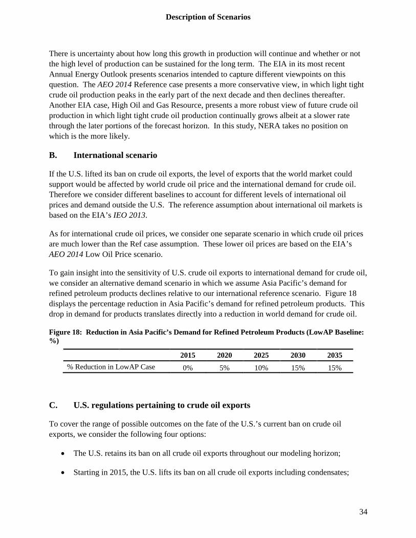
Description of Scenarios
34
There is uncertainty about how long this growth in production will continue and whether or not the high level of production can be sustained for the long term. The EIA in its most recent Annual Energy Outlook presents scenarios intended to capture different viewpoints on this question. The AEO 2014 Reference case presents a more conservative view, in which light tight crude oil production peaks in the early part of the next decade and then declines thereafter. Another EIA case, High Oil and Gas Resource, presents a more robust view of future crude oil production in which light tight crude oil production continually grows albeit at a slower rate through the later portions of the forecast horizon. In this study, NERA takes no position on which is the more likely.
B. International scenario
If the U.S. lifted its ban on crude oil exports, the level of exports that the world market could support would be affected by world crude oil price and the international demand for crude oil. Therefore we consider different baselines to account for different levels of international oil prices and demand outside the U.S. The reference assumption about international oil markets is based on the EIA’s IEO 2013.
As for international crude oil prices, we consider one separate scenario in which crude oil prices are much lower than the Ref case assumption. These lower oil prices are based on the EIA’s AEO 2014 Low Oil Price scenario.
To gain insight into the sensitivity of U.S. crude oil exports to international demand for crude oil, we consider an alternative demand scenario in which we assume Asia Pacific’s demand for refined petroleum products declines relative to our international reference scenario. Figure 18 displays the percentage reduction in Asia Pacific’s demand for refined petroleum products. This drop in demand for products translates directly into a reduction in world demand for crude oil.
Figure 18: Reduction in Asia Pacific’s Demand for Refined Petroleum Products (LowAP Baseline: %)
2015 2020 2025 2030 2035 % Reduction in LowAP Case 0% 5% 10% 15% 15%
C. U.S. regulations pertaining to crude oil exports
To cover the range of possible outcomes on the fate of the U.S.’s current ban on crude oil exports, we consider the following four options:
• The U.S. retains its ban on all crude oil exports throughout our modeling horizon;
• Starting in 2015, the U.S. lifts its ban on all crude oil exports including condensates;

Description of Scenarios
35
• An alternative policy option suggested by some is a partial lifting of the ban on crude oil exports which would allow condensate (API gravity >49) to be exported but no other lower gravity crude oils. This scenario assumes the U.S. lifts the export ban on only condensates starting in 201525; and
• The fourth option considers a delay in lifting the ban on all crude oil exports until 2020.
D. OPEC response
Questions have been raised about how OPEC will respond to the larger volume of crude oil on the international market if the U.S. allows exports of its crude oil production. We considered three possible responses for OPEC:
• OPEC reduces production to maintain world crude oil prices;
• OPEC keeps its production at the same levels as if the ban remained in effect; and
• OPEC behaves as a competitive supplier and produces at levels that are consistent with its supply curve and the new market conditions.
E. Summary of all cases
Figure 19 presents the different combinations of assumptions that were assumed in the eighteen cases we analyzed. The five baseline cases, which assume the ban remains in effect, capture the different possibilities for both the U.S. and the international crude oil market. While the thirteen scenarios consider different assumptions for the way in which the crude oil export ban is lifted, the market environment in which it is lifted, and OPEC’s response.
The cases are arrayed in Figure 18 to clarify the baseline against which each scenario is analyzed. The five different baselines, in which there is a crude oil export ban, are designated in Bold. The scenarios compared to those baselines follow each. The scenarios vary in the type of crude oil export ban, OPEC’s response to the U.S. modifying its crude oil export ban, and Asia Pacific’s demand for refined petroleum products. The scenarios under the Ref and HOGR baselines, which are highlighted, encompass the range of modifications to the crude oil export ban that we considered. The cases not highlighted under the Ref and HOGR cases contain sensitivities around the complete lifting of the ban in 2015. The three different U.S. cases are separated by double lines. Each U.S. case has different baseline assumptions affecting U.S. crude oil supply (Ref, HOGR, and LOP). A more detailed exposition of the various scenarios is provided in Appendix D.
25 In this scenario, we adopt the definition and data on condensates from the EIA AEO 2014. See footnote 17 above
for a discussion of recent Department of Commerce rulings on export of condensate produced by two companies.

Description of Scenarios
36
Figure 19: Summary of Scenarios Analyzed in this Study
US Case Baselines/Scenarios Crude Oil Exports
Banned OPEC
Response Asia Pacific
Demand
Ref
Ban_Ref All N/A Reference NoBanCond_Ref All except Condensates Market Reference
NoBan_Ref None Market Reference NoBanDelay_Ref None from 2020 onward Market Reference
NoBanOPECCut_Ref None Cut Exports Reference NoBanOPECFix_Ref None Fix Exports Reference
BanLowAP_Ref All N/A Low NoBanLowAP_Ref None Market Low
HO
GR
Ban_HOGR All N/A Reference NoBanCond_HOGR All except Condensates Market Reference
NoBan_HOGR None Market Reference NoBanDelay_HOGR None from 2020 onward Market Reference
NoBanOPECCut_HOGR None Cut Exports Reference NoBanOPECFix_HOGR None Fix Exports Reference
BanLowAP_HOGR All N/A Low NoBanLowAP_HOGR None Market Low
LO
P Ban_LOP All N/A Reference NoBan_LOP None Market Reference

Global Petroleum Model Results
37
IV. GLOBAL PETROLEUM MODEL RESULTS
For this study, NERA developed two primary26 baselines for the world: Ban_Ref and Ban_HOGR. The baselines differ most for the U.S. as they primarily differ in their assumptions about the availability of U.S. crude oil resources. This difference leads to moderate differences in world energy prices. The next section reports for the U.S. the crude oil production, average wellhead crude oil price, and total demand for refined petroleum products.
A. The NERA U.S. Baseline
For the U.S., the Ref baseline is based upon but not precisely calibrated to the EIA’s AEO 2014 Reference case. NERA’s HOGR baseline is based upon, but not calibrated to the EIA’s AEO 2014 High Oil and Gas Resource case. Figure 20 and Figure 21 report key U.S. metrics of the two NERA baselines.
Figure 20: NERA’s Ref Baseline for U.S. Crude Oil Production, Average Wellhead Crude Oil Price, and Demand for Refined Petroleum Products
2015 2020 2025 2030 2035
Crude Oil Production (MBD)
9.0 10.0 10.4 9.9 9.5
Wellhead Price (Lower 48) ($/bbl)
$83 $83 $97 $109 $121
U.S. RPP Demand (MBD)
17.2 17.5 17.2 16.8 16.5
26 From these two core baselines, we developed two alternative baselines (BanLowAP_Ref and BanLowAP_HOGR)
that accounted for the effects on the U.S. crude oil market from lower demand for refined petroleum products in the Asia Pacific region. We also developed a fifth baseline (Ban_LOP) based on the AEO’s 2014 Low Oil Price case.

Global Petroleum Model Results
38
Figure 21: NERA’s HOGR Baseline for U.S. Crude Oil Production, Average Wellhead Crude Oil Price, and Demand for Refined Petroleum Products
2015 2020 2025 2030 2035
Crude Oil Production (MBD)
9.3 10.7 11.7 11.8 11.9
Wellhead Price (Lower 48) ($/bbl)
$79 $76 $84 $91 $99
Indigenous RPP Demand (MBD)
19.2 20.0 19.7 19.3 19.2
B. Scenario Results
Impacts for the different scenarios are all presented relative to a baseline in which the crude oil export ban remains in effect. Most of the scenario results are presented relative to the Ban_Ref and Ban_HOGR baselines. The Asia-Pacific results are presented against the BanLowAP_Ref and BanLowAP_HOGR baselines which are different than the Ban_Ref and Ban_HOGR baselines only in the level of refined petroleum product demand in the Asia-Pacific region. The Low Oil Price scenario (LOP), in which the ban is lifted, is presented against a baseline which maintains the crude oil export ban, but assumes a much lower world-wide crude oil price ($70/bbl-$75/bbl) than in the Ban_Ref and Ban_HOGR baselines.
The remainder of this chapter is organized into three sections. The first section presents results for the scenarios in which the crude oil export ban is completely lifted in 2015 (NoBan_Ref and NoBan_HOGR). It discusses in detail the impacts on crude oil exports, U.S. crude oil production, U.S. and rest of world crude oil prices, refined petroleum product prices in the U.S. and rest of world, refined petroleum product exports and the impact on refiner’s margins.
The second section compares the impacts from alternative proposals for lifting the crude oil export ban relative to the scenario in which the ban is completely lifted in 2015 (NoBanDelay_Ref, NoBan2020_Ref, NoBanCond_Ref, NoBanDelay_HOGR, NoBan2020_HOGR, and NoBanCond_HOGR). The alternatives consider either a partial lifting of the ban or a delay in the date for completely lifting the crude oil export ban.
The third section assesses the importance of alternative environments in which the ban is lifted (NoBan_LowAP_Ref, NoBanOPECCut_Ref, NoBanOPECCut_Ref, NoBan_LowAP_HOGR, NoBan_OPECCut_HOGR, NoBan_OPECFix_HOGR, and NoBan_LOP). These alternative environments consist of different responses by OPEC to lifting the crude oil export ban, low

Global Petroleum Model Results
39
world-wide crude oil prices, and slower-than-expected growth in refined petroleum product demand in Asia-Pacific.
1. Complete Lifting of the Crude Oil Export Ban in 2015
This first section of the results discusses the impacts on the various sectors of the petroleum industry from a complete lifting of the crude oil export ban in 2015.
a. Crude Oil Price Spreads
Lifting of the crude oil export ban allows crude oil produced in the U.S. to compete in the global market and receive value commensurate with the global price of crude oil. In the U.S., lifting the crude oil export ban will provide a means for more U.S. light tight oil to come to market. When the ban is in place, with a few exceptions crude oil produced in the U.S. can only be utilized by U.S. refineries. But these refineries lack the capacity to process all the light tight crude oil that the U.S. can produce at world market prices. Therefore, when the export ban is in place, light tight crude oil sells at a large discount to intermediate crude oil. In 2015 the differential in both the Ref and HOGR cases is about $20, and its path thereafter mirrors the change in U.S. production of light tight oil -- falling in Ref and rising in HOGR (see Figure 22 and Figure 23).
When the export ban is lifted, U.S. light tight crude oil prices will increase and consequently reduce the price spreads between light tight and intermediate crude oils. Figure 22 illustrates this point. In the Ref case, we estimate a lifting of the crude oil export ban would reduce the price spread between light tight oil and intermediate crude oil by $15/bbl in 2015 and by $1.90/bbl in 2035. With the ban remaining in effect, the price spread reaches as much as $21/bbl. With the ban completely lifted in 2015, the price of light tight crude oil increases by between $1.80/bbl and $12/bbl. Although the prices of most crude oil types in the U.S. actually decrease by up to $3.90/bbl, the greater increases in light tight crude oil and condensate prices result in the average price of crude oil in the U.S. increasing by as much as $3.50/bbl.

Global Petroleum Model Results
40
Figure 22: U.S. ICRU-U.S. LTO Price Spread with and without the Crude Oil Export Ban in Place (Ref Baseline: 2013$/bbl)
Figure 23 shows that for the HOGR scenario directionally the same effect on prices spreads, but the spreads decline by a larger magnitude than in the Ref scenario. With the ban remaining in effect the price spread grows to $34/bbl in 2035. Unlike the Ref, the price spread increases in the outer years because the U.S. resource potential is assumed to grow over time. With the crude oil export ban lifted, the price spread shrinks to $1.40/bbl by 2035, a level more comparable to the Ref scenario. Thus in the long-run the spread converges to the assumed cost difference between processing light tight crude oil and intermediate crude oil. In the HOGR case, the export ban causes the price of light tight crude oil to be depressed even further relative to the price of intermediate crude oil – from $23 to $34 per barrel from 2015 to 2035, so that lifting the ban produces an even larger increase in the price of light tight crude oil.
$0
$5
$10
$15
$20
$25
$30
$35
2015 2020 2025 2030 2035
$/bb
l
Ban_Ref NoBan_Ref

Global Petroleum Model Results
41
Figure 23: U.S. ICRU-U.S. LTO Price Spread with and without the Crude Oil Export Ban in Place (HOGR Baseline: 2013$/bbl)
The other factor that drives the production of additional light tight crude oil in the U.S. is the price spread between light tight crude oil inside versus outside the U.S. Just as the price spread narrows in the U.S. between LTO and ICRU when the ban is lifted so does the price spread between U.S. LTO and LTO in the rest of the world. In the Ref case, the LTO in the U.S. sells at a $16 discount to international LTO. This discount shrinks over time as the U.S. resource of light tight oil becomes exhausted with time. When the ban is lifted, the differential between U.S. and rest of the world LTO prices virtually vanishes because U.S. light tight crude oil can freely compete with the same grade of crude oil produced outside the U.S. It returns in the later years because of the interplay between crude oil production throughout the world, world refinery capacity, and world demand for refined petroleum products (Figure 24).
$0
$5
$10
$15
$20
$25
$30
$35
2015 2020 2025 2030 2035
$/bb
l
Baseline (ban remains in-effect) Crude Oil Export Ban Lifted in 2015

Global Petroleum Model Results
42
Figure 24: International LTO-U.S. LTO Price Spread with and without the Crude Oil Export Ban in Place (Ref Baseline: 2013$/bbl)
As with the Ref case, the spread between the international and U.S. light tight crude oil prices mirrors the spread between U.S. LTO and ICRU in the HOGR. When the export ban is in place the spread is comparable to the 2015 value for the Ref case, but then it steadily increases as the light tight crude oil resource becomes more developed. When the ban is removed, the price spread under the HOGR tracks closely with the price spread under the Ref case with the ban removed. Figure 25 shows the spread between international and U.S. light tight crude oil prices with and without the ban in the HOGR cases.
$0
$5
$10
$15
$20
$25
$30
$35
2015 2020 2025 2030 2035
$/bb
l
Baseline (ban remains in-effect) Crude Oil Export Ban Lifted in 2015

Global Petroleum Model Results
43
Figure 25: International LTO-U.S. LTO Price Spread with and without the Crude Oil Export Ban in Place (HOGR Baseline: 2013$/bbl)
b. U.S. Crude Oil Production
With the complete lifting of the crude oil export ban, the demand for U.S. light tight crude oil and condensate increases, which causes an increase in the price for these crude oils. The higher price will cause more of the resource to become economic to develop. As a result, drilling and production of light tight crude oil and condensate will increase. Figure 26 shows the net increase in total U.S. production of crude oil. The Ref scenario production peaks in 2020 consistent with the AEO Reference case’s underlying assumption about the U.S. resource base being more limited. The HOGR scenario shows incremental production increasing with time consistent with the AEO’s HOGR case’s underlying assumption that the resource is abundant and economic prospects increase with time as the technology develops and the resource becomes better defined.
The consistent picture for 2015 from both scenarios is that U.S. crude oil production would be between 1.5 and 2 million barrels per day higher were it not for the ban on crude oil exports.
$0
$5
$10
$15
$20
$25
$30
$35
2015 2020 2025 2030 2035
$/bb
l
Baseline (ban remains in-effect) Crude Oil Export Ban Lifted in 2015

Global Petroleum Model Results
44
Figure 26: Incremental Crude Oil Production Resulting from the Complete Lifting of the Crude Oil Export Ban in 2015 (Ref and HOGR Baselines: MBD)
The increase in U.S. crude oil supplies is attributable almost entirely to greater production of light tight crude oil and condensate. Thus the location of light tight crude oil and condensate fields will determine the PADDs that will enjoy the greatest increase in crude oil production. Utica, Bakken, Eagle Ford, Permian, and Niobrara are the basins that are expected to be the large sources of light tight crude oil and condensate. These basins are located in PADDs 2, 3 and 4, respectively. As Figure 27 shows, these PADDs will enjoy the greatest increase in production. The greater production in PADD 3 compared to PADD 2 in 2015 combines with increased infrastructure to alleviate constraints and regional pricing disparities within the U.S., by moving production closer to Gulf Coast refineries.
0.0
1.0
2.0
3.0
4.0
5.0
2015 2020 2025 2030 2035
MB
D
REF HOGR

Global Petroleum Model Results
45
Figure 27: Distribution of Incremental Crude Oil Production by PADD in 2015 Resulting from the Complete Lifting of the Crude Oil Export Ban in 2015 (Ref and HOGR Baselines: MBD)
c. Net Imports of Crude Oil
Even with the lifting of the crude oil export ban, the U.S. will remain a net importer of crude oil. The U.S. currently imports 7.7 MBD27 of crude oil and exports about 0.3 MBD of crude oil. Lifting of the ban will have a substantial impact on the level of crude oil exports and a small impact on crude oil imports. Furthermore, lifting of the ban will alter the mix of crude oils that are both imported and exported.
The principal effect of lifting the ban is to allow the export of light tight crude oil and condensate produced in the U.S. that does not have an economic market in the U.S. The magnitude of crude oil exports will be determined by the outlook for the resource with the HOGR scenario having the greater level of exports than the Ref scenario.
Figure 28 shows the change in crude oil exports and imports as well as the change in net crude oil imports for the Ref scenario. The purple (positive) bars represent the change in gross exports, the orange (positive) bars represent the change in gross imports, and their difference expressed as the change in net imports (equal to change in gross exports minus change in gross imports) is in green (orange bar less purple bar). In the Ref case, imports and exports increase in 2015 - 2035 27 2013 value http://www.eia.gov/dnav/pet/hist/LeafHandler.ashx?n=PET&s=MCRIMUS1&f=A
0.0
0.2
0.4
0.6
0.8
1.0
1.2
1.4
1.6
PADD 1 PADD 2 PADD 3 PADD 4 PADD 5
MB
D
REF HOGR

Global Petroleum Model Results
46
as U.S. refiners exercise their greater flexibility in purchasing to better optimize the mix of crude oils for their refineries, and on balance net imports fall as the U.S. increases exports more than imports because lifting the band frees up more supply for export.
By 2030 - 2035, increased exports of light tight crude oil and condensate are offset by increased imports of heavier crude oils, so that inputs of crude oil to refineries are better matched to existing refinery capabilities and investments in upgrading to handle light tight crude oil are avoided. This frees resources for other, more productive investments. The change in net crude oil imports converges toward zero as the supply of light oils declines.
A different pattern over time is seen in Figure 28 which shows the change in crude oil exports and imports as well as net imports for the HOGR scenario. In this scenario, reductions in net imports become larger with time as the U.S. crude oil resource base is more abundant and able to sustain higher levels of crude oil production over time.
Figure 28: Change in Crude Oil Export and Imports Resulting from the Complete Lifting of the Crude Oil Export Ban in 2015 (Ref Baseline: MBD)
-6
-5
-4
-3
-2
-1
0
1
2
3
4
5
6
2015 2020 2025 2030 2035
MB
D
Change in Exports Change in Imports Change in Net Imports

Global Petroleum Model Results
47
Figure 29: Change in Crude Oil Export and Imports Resulting from the Complete Lifting of the Ban in 2015 (HOGR Baseline: MBD)
In both the Ref and HOGR cases, the U.S. remains a net importer of crude oil in all the scenarios, and net imports of crude oil are reduced in all years.
The consistent pattern of increase in gross crude oil imports suggests that the immediate impact of allowing crude oil exports is to allow production of light tight crude oil to grow beyond the optimal input levels desired by U.S. refineries, and that U.S. refineries switch some of their purchases from light domestic crude oil to imports of heavier crude oils for which their configuration is better suited. Exports also make it possible to optimize global refinery utilization by allowing export of U.S. light tight crude oil and condensate to regions where it is most valuable.
The relationship between exports, imports, refinery demand and production of crude oil is illustrated in the following two figures (Figure 30 and Figure 31). Supply and demand for crude oil must balance, and so must the change in supply and demand. Exports and refinery consumption represent sources of demand for crude oil. Imports and crude oil production represent sources of supply. Therefore increases in production equal any increases in exports plus any increases in refinery demand less any increases in imports.
The two figures show that the increase in incremental exports can exceed the increase in incremental production by the difference in incremental refinery demand and incremental imports.
-6
-5
-4
-3
-2
-1
0
1
2
3
4
5
6
2015 2020 2025 2030 2035
MB
D
Change in Exports Change in Imports Change in Net Imports

Global Petroleum Model Results
48
Figure 30: Waterfall Chart Showing the Change in U.S. Exports, Imports, Consumption and Production of Crude Oil Resulting from the Complete Lifting of the Ban in 2015 (Ref Baseline: MBD)
Figure 31: Waterfall Chart Showing the Change in U.S. Exports, Imports, Consumption and Production of Crude Oil Resulting from the Complete Lifting of the Ban in 2015 (HOGR Baseline: MBD)
-1.0
0.0
1.0
2.0
3.0
4.0
5.0
6.0
Expo
rts
Con
sum
ptio
n
2015
Im
ports
Prod
uctio
n
Expo
rts
Con
sum
ptio
n
2035
Im
ports
Prod
uctio
n
Cha
nge
in Q
uant
ity (
MB
D)
0
1
2
3
4
5
6
Expo
rts
Con
sum
ptio
n
2015
Im
ports
Prod
uctio
n
Expo
rts
Con
sum
ptio
n
2035
Im
ports
Prod
uctio
n
Cha
nge
in Q
uant
ity (
MB
D)

Global Petroleum Model Results
49
d. ROW Crude Oil Price and Production Impacts
U.S. exports of crude oil increase world supply and therefore decrease average world-wide crude oil prices. The ban on crude oil exports prevents U.S. produced light tight crude oil and condensate from reaching the world market and causes world crude oil prices to be inflated. Figure 32 shows the decline in crude oil prices outside the U.S. for both the Ref and the HOGR scenarios. Whereas in Ref the largest impact is on world oil prices in 2015, declining over the years as light tight crude oil production peaks and falls off in the US, in the HOGR case the reduction in world oil prices holds at about $6 to $7 per barrel all the way out to 2035 because light tight crude oil production is maintained.
Figure 32: Change in Average Crude Oil Price for Rest of World from the Complete Lifting of the Ban in 2015 (Ref and HOGR Baselines: 2013$/bbl)
The lifting of the crude oil export ban will result in more U.S. crude oil production that will be absorbed in the world market. This absorption will occur by some combination of increased demand and reduced crude oil production in the rest of the world. We find that the reduction in production and the increased in demand from the rest of the world are about equal, so that displacement and demand creation are about equal (Figure 33).
-$8
-$7
-$6
-$5
-$4
-$3
-$2
-$1
$02015 2020 2025 2030 2035
$/bb
l
REF HOGR

Global Petroleum Model Results
50
Figure 33: Distribution of U.S. Crude Oil Exports in the World Market Resulting from the Complete Lifting of the Ban in 2015 (Ref and HOGR Baselines: MBD)
2015 2020 2025 2030 2035
Ref (MBD)
U.S. Total Exports 1.7 1.9 1.6 1.7 1.1 ROW Displacement 1.0 0.9 0.4 0.1 0.0 ROW Demand Increase 0.7 1.0 1.2 1.5 1.1
HOGR (MBD)
U.S. Total Exports 2.5 3.6 4.2 4.5 5.2 ROW Displacement 1.4 1.7 2.0 2.5 2.6 ROW Demand Increase 1.1 1.9 2.2 2.1 2.6
e. Rest of World Refined Petroleum Product Price
Crude oil cost is the chief contributor to refined petroleum product prices, aside from taxes in some parts of the world. Lowering the cost of crude oil worldwide lowers the cost of producing refined petroleum products and thus their prices. A relatively small decline in crude oil prices world-wide will result in a small decline in gasoline prices. For the Ref scenario, the decline in international gasoline prices starts at $0.09/gallon in 2015 and almost disappears by 2035. In the HOGR scenario, the gasoline price declines by $0.013/gallon in 2015 and falls by$0.08/gallon in 2035. The trajectory of the declines differ between the Ref and HOGR cases because the cases have much different forecasts for the availability of crude oil resources over time. Since the Ref forecasts the increase in light oil peaks around 2020 and declines afterward, the U.S. exports have little effect on international markets by the end of the horizon. Under HOGR, however, the production of light crude oils is forecasted to increase through much of the time horizon so this supports higher levels of crude oil throughout the horizon and hence lower crude oil and refined petroleum product prices.
f. U.S. Refined Petroleum Product Price
Even though crude oil cannot currently be exported from the lower 48 (with a few exceptions); there is no limitation on either the import or export of refined petroleum products. On balance, the U.S. is a net exporter of refined petroleum products, but depending on the type of refined petroleum product and PADD, the U.S. is both an importer and an exporter. As a result, the U.S. is linked to the global market, and it is the global market that determines the price of refined petroleum products in the U.S. In this global interconnected market, differences in prices between regions are determined by differences in refining and transportation costs. Thus U.S.

Global Petroleum Model Results
51
prices for refined petroleum products move together with refined petroleum product prices in other regions of the world.28
Figure 34 presents the change in average gasoline prices in the U.S. resulting from the lifting of the crude oil export ban. For the Ref scenario where the entire ban is lifted in 2015, the average U.S. gasoline price declines the most in 2015 ($0.09/gal) and tapers off to nearly zero by 2035. In the HOGR scenario where the entire ban is again lifted in 2015, the U.S. average gasoline price again declines the most in 2015 ($0.12/gal), but the continued increase in U.S. production of light tight crude oil and condensates causes U.S. production to increase through 2035 and these additional supplies force down gasoline prices through this time period. Under all scenarios, the retail gasoline price decreases when the ban is lifted.
Figure 34: Change in the U.S. Gasoline Prices Resulting from the Complete Lifting of the Ban in 2015 (Ref and HOGR Baselines: 2013$/gal)
g. U.S. Exports of Refined Petroleum Products
Lifting the crude oil export ban will raise the price of light tight crude oil and condensate in the U.S. and lower the average price of crude oil world-wide. The higher price for light tight crude
28 Stephen P.A. Brown, Charles Mason, Alan Krupnick, and Jan Mares, “Crude Behavior: How Lifting the Export
Ban Reduces Gasoline Prices in the United States,” Resources for the Future, Issue Brief 14-03-REV, February 2014, revised March 2014, .
-$0.14
-$0.12
-$0.10
-$0.08
-$0.06
-$0.04
-$0.02
$0.002015 2020 2025 2030 2035
$/ga
l
REF HOGR

Global Petroleum Model Results
52
oil and condensate in the U.S. increases the average cost of crude oil supplies to some U.S. refiners and hence their cost to produce refined petroleum products will rise. Lower world-wide crude oil prices will lower the cost to produce refined petroleum products outside the U.S. As a result, U.S. refiner’s competitive advantage relative to refiners in other regions of the world will diminish. Although the U.S. is both an importer and exporter of refined petroleum products, most of the resulting change takes the form of a reduction in exports. Product imports increase only slightly in the peak year when crude oil exports are allowed. Figure 35 presents the change in exports of refined petroleum products from the U.S. for the Ref and HOGR scenarios when the crude oil export ban is lifted in 2015.
Figure 35: Change in U.S. Refined Petroleum Product Exports and Imports Resulting from the Complete Lifting of the Ban in 2015 (Ref and HOGR Baselines: MBD)
2015 2020 2025 2030 2035
Total RPP Ref (MBD)
Exports -0.1 -0.3 -0.4 -0.4 -0.4 Imports 0.0 0.0 -0.1 0.0 0.1 Net Exports -0.2 -0.3 -0.3 -0.3 -0.5
Total RPP HOGR (MBD)
Exports -0.2 0.0 -0.3 -0.1 0.0 Imports 0.0 0.2 -0.1 0.0 0.0 Net Exports -0.2 -0.2 -0.3 -0.1 -0.1
h. U.S. Refineries
Higher crude oil prices and lower refined petroleum product prices will reduce some U.S. refiners' gross margins. Since imported refined petroleum products, in particular gasoline, set the price of those products in the U.S., increases in U.S. crude oil prices will not be felt by U.S. consumers, but they will erode the gross margins of some refiners. Furthermore, allowing light tight crude oil to reach its global value by allowing its export from the U.S. will increase its price. Those refiners who have been able to get access to light tight crude oil and are including it in their crude oil mix will experiences additional downward pressure on their gross refinery margins.
Simultaneously, the demand for refined petroleum products in the U.S. will increase slightly due to lower global prices for refined petroleum products, but exports will decline as a result of the change in the competitive position of U.S. refiners versus foreign refineries. As a result, U.S. refiners will be producing slightly less refined petroleum products than they would with the export ban, but they will be exporting less and delivering more to domestic customers. The net impacts on refinery output can be seen in Figures 29 and 30 above. Since consumption of crude oil is a measure of refinery throughput, they show that in total refinery throughput could fall by from 0 -100,000 barrels per day in 2015 and from 0 - 300,000 barrels per day in 2030. Those numbers represent from 0 - 1% of total refinery throughput in 2015 and 0 - 2% in 2035.

Global Petroleum Model Results
53
The reason for the small impacts on refinery output in the U.S. is that any reductions in refinery margins will be a downward adjustment in margins to return them to a level closer to their historic averages. Figure 36 shows that over the period from 2000 to 2013 refinery gross margins averaged about $17 dollars per barrel. With the increase in crude oil prices and reduction in refined petroleum product prices, the average gross refiner margin will fall. Individual refiners will experience this reduction in margins to different degrees, but on average the decline in refiners’ margins will leave them with margins slightly less than the average for the past 14 years.
Figure 36 shows the historic gross refiner’s margin and the model prediction of gross refiner margin when the crude oil export ban remains in effect. Refiners’ gross margins have fluctuated substantially from year to year as a result of changes in market conditions. The model calculated gross margin assumes a more stable market conditions and calculates a gross margin within the range of historic margins.
Figure 36: Historical U.S. Refinery Gross Margin and Forecasted U.S. Refinery Gross Margins under Different Assumptions about the U.S. Crude Oil Export Ban and Availability of U.S. Crude Oil Resources (Ref and HOGR Baselines: 2013$/bbl) 29
29 Historical data is from calculations using historical U.S. production and prices found on the EIA website.
$0
$5
$10
$15
$20
$25
$30
Ref
iner
y G
ross
Mar
gins
($/b
bl)
Historical Ref Ban Case Ref No Ban CaseHOGR Ban Case HOGR No Ban Case
Historical Future

Global Petroleum Model Results
54
2. How Market Forces Impact Crude Oil Exports
Concerns have been raised about other independent factors that might affect the impacts from lifting the crude oil export ban in 2015. These other factors range from the response by OPEC to the U.S. actions and the impact of other developments in the market that are unrelated to the lifting of the ban but may have an effect on the energy market’s response to the lifting of the ban. In this section, we present our analysis of several of these selected factors.
a. Potential OPEC Responses
OPEC can respond to the U.S. lifting of its crude oil export ban in one of three ways:
1. Continue to behave as a competitive supplier on the world market, adjusting its production up and down in response to price changes over which it exercises no control;
2. Maintain its export levels at the levels projected for the scenario with an export ban in place; or
3. Reduce exports in an attempt to maintain crude oil prices at a level they would reach with an export ban in place.
Although there have been many theories about OPEC behavior, including the theory that OPEC is incapable of coordinated action, one factor that OPEC might consider is the impact of an option on export revenues. Thus we calculated OPEC’s forecasted annual oil export revenues for each of the above three options and the baseline in which the crude oil export ban remains in effect. These calculations are presented in Figure 37 and Figure 38 for complete lifting of the ban in 2015 for the Ref and HOGR cases, respectively. Since the time profile of impacts differs between the Ref and HOGR cases, the Figure 37 and Figure 38 report levelized annual revenues, calculated by dividing the net present value of OPEC revenues by the number of years from 2015 to 2035. Figure 37: Annualized OPEC Revenues from Petroleum Exports (Ref Baseline: Billion 2013$s)
Scenario 2015 NPV/year
Net Crude Oil Exports (billion 2013$s/year)
Baseline $353 Competitive Supplier $343
Maintain Export Levels $349 Maintain Crude Oil Prices $332

Global Petroleum Model Results
55
Figure 38: Annualized OPEC Revenues from Petroleum Exports (HOGR Baseline: Billion 2013$s)
Scenario 2015 NPV/year
Net Crude Oil Exports (billions 2013$s/year)
Baseline $363 Competitive Supplier $331
Maintain Export Levels $347 Maintain Crude Oil Prices $293
In the Ref case, the difference in revenue across the three options is just $17 billion per year, but in the HOGR case it is $54 billion. In both cases, OPEC’s revenues are lowest if it should try to maintain world crude oil prices by cutting exports, and highest if it maintains production levels at the same target it would choose in the baseline. The small difference that OPEC’s response can make in the Ref case suggests that it is likely OPEC would simply ignore U.S. exports in that case, since normal market variations have produced much larger swings in OPEC revenues in the past with no coordinated response. In the HOGR case, the response of cutting production would reduce OPEC revenues by over 10% compared to doing nothing, and the prospect that OPEC could manage a coordinated response that would reduce its revenues that substantially just to punish the U.S. for entering as a competitor seems farfetched.
Therefore, the unlikely worst outcome that OPEC could impose on the U.S. is one with no change in global crude oil prices or U.S. gasoline prices. As additional supplies enter the market, OPEC has the choice of cutting back production to maintain the price or maintaining production levels and letting the price fall. If OPEC attempts to maintain exports at the levels assumed in the export ban case, that assures the largest drop in world oil prices and in U.S. gasoline prices. If OPEC cuts back production, the price reduction will be moderated.
But if OPEC cuts production, it would confer a substantial security benefit, in that less oil would be produced in the Persian Gulf and subject to interruption due to war or civil conflict and less oil would be produced and less revenue would flow to regions that are vulnerable to supply disruptions. This could be an even bigger long run benefit than the reductions in gasoline prices predicted when OPEC maintains production.

Global Petroleum Model Results
56
Figure 39: Change in OPEC’s Exports of Crude Oil Resulting from a Complete Lifting of the Ban in 2015 under Different Assumptions about OPEC’s Actions (Ref and HOGR Baselines: %)
These OPEC responses illustrate the win-win nature of allowing crude oil exports from the U.S. – if the U.S does not realize a lower refined petroleum product price, the U.S. would still win on energy security.
b. Low Crude Oil Price Outlook
The scenarios examined above all assume that current world crude oil prices are sustainable and increase with time. An alternative view of the future is one in which crude oil prices adjust downward and remain low throughout the forecast horizon. This study examines such a case, which is based upon the EIA’s AEO 2014 Low Oil Price case. The low oil price scenario assumes that greater levels of exports from the Middle East (OPEC) and slower than expected economic growth in some regions of the world result in a world-wide crude oil price trajectory that begins at about $70/bbl in 2015 and rises to less than $75/bbl in 2035. Against this backdrop, we analyze two scenarios: one in which the crude oil export ban remains in place and one in which the export ban is lifted in 2015.
As discussed earlier the principal effect of lifting the crude oil export ban is that it allows light tight crude oil and condensate to be sold into a higher valued market. This results in higher prices for light tight oil and condensate, which in turn stimulates more drilling and production of crude oil, which can be exported outside the U.S.
If the world market is not higher valued, then there is no incentive for more production. In the Low Oil price scenario, the crude oil price spread that stimulates more production is nearly eliminated even with the crude oil export ban in place, and the price for light tight oil is not significantly higher than the minimum required to make production economic from shale. As a result, lifting the ban yields only a minimal amount of additional production, which translates into little change in crude oil exports and a minimized effect on crude oil and refined petroleum
-25%
-15%
-5%
2015 2020 2025 2030 2035
Perc
ent C
hang
e in
OPE
C E
xpor
ts
NoBanOPECCut NoBanOPECFixRef
2015 2020 2025 2030 2035
NoBanOPECCut NoBanOPECFix
HOGR

Global Petroleum Model Results
57
product prices. As shown in Figure 40, the level of total light tight crude oil and condensate exports resulting from the lifting of the ban is less than 0.2 MBD in any year.
Figure 40: U.S. Light Tight Crude Oil and Condensate Exports Resulting from the Complete Lifting of the Ban in 2015 (Low Oil Price Baseline: MBD)
2015 2020 2025 2030 2035 Gross Crude Oil Exports (MBD) Ban Lifted in 2015 0.19 0.05 0.00 0.00 0.00
c. Lower than Expected Growth in the Asia-Pacific Region
The Asia-Pacific region represents the major growth market for petroleum. Therefore, a question arises about the potential for U.S. exports if the Asia-Pacific market grows at a rate below expectations. To address this question, this study considers a scenario in which the Asia-Pacific region demand for refined petroleum products is up to 15% lower than in the other baselines. A scenario assuming this lower growth in Asia-Pacific combined with the crude oil export ban in place is compared to a scenario of the same lower demand except the crude oil export ban is completely lifted in 2015. The comparison of the results for the international reference ({default}) and LowAP are presented in Figure 41 and Figure 42.
These figures indicate that U.S. net crude oil imports would be about 0.2 MBD less than if Asia-Pacific refined petroleum product demand grew at expected rates in 2025. Furthermore, crude oil prices in the rest of the world at the time of maximum increase in U.S. exports would be $1.10 less. Even so, the gasoline price benefit in the U.S. would be nearly zero.

Global Petroleum Model Results
58
Figure 41: Impact of Completely Lifting the Ban in 2015 as a function of Asia Pacific’s Demand for Refined Petroleum Products (Ref Baseline)
2015 2020 2025 2030 2035
U.S. Gross Crude Oil Exports relative to baselines (MBD)
Asia-Pacific Reduced Demand 1.7 1.8 1.6 1.4 1.0 Asia-Pacific Reference Demand30 1.7 1.9 1.6 1.7 1.1 Difference 0.0 0.0 -0.1 0.2 0.1
U.S. Net Imports of Crude Oil (MBD)
Asia-Pacific Reduced Demand 5.7 6.0 6.8 7.5 7.9 Asia-Pacific Reference Demand 5.7 6.0 7.1 7.4 7.8 Difference 0.0 0.1 0.2 -0.1 -0.1
Change in ROW Crude Oil Price (2013$/bbl)
Asia-Pacific Reduced Demand -$3.80 -$1.67 -$0.63 -$0.17 -$0.07 Asia-Pacific Reference Demand -$3.80 -$2.02 -$0.70 -$0.19 -$0.07 Difference $0.00 -$0.35 -$0.07 -$0.02 $0.00
Change in U.S. Gasoline Prices (2013$/bbl)
Asia-Pacific Reduced Demand -$0.09 -$0.03 -$0.01 $0.00 $0.00 Asia-Pacific Reference Demand -$0.09 -$0.04 $0.00 $0.00 $0.00 Difference $0.00 -$0.01 $0.01 $0.00 $0.00
Figure 42: Impact of Completely Lifting the Ban in 2015 as a function of Asia Pacific’s Demand for Refined Petroleum Products (HOGR Baseline)
2015 2020 2025 2030 2035
U.S. Gross Crude Oil Exports relative to baselines (MBD)
Asia-Pacific Reduced Demand 2.5 3.4 4.1 4.4 5.1 Asia-Pacific Reference Demand31 2.5 3.6 4.2 4.5 5.2
Difference 0.0 0.2 0.1 0.1 0.1
U.S. Net Imports of Crude Oil (MBD)
Asia-Pacific Reduced Demand 5.0 4.7 3.7 3.5 3.0 Asia-Pacific Reference Demand 5.0 4.4 3.9 3.5 3.1 Difference 0.0 -0.3 0.2 0.0 0.1
Change in ROW Crude Oil Price (2013$/bbl)
Asia-Pacific Reduced Demand -$5.94 -$4.79 -$5.61 -$5.04 -$4.86 Asia-Pacific Reference Demand -$5.94 -$5.38 -$5.71 -$6.14 -$6.87 Difference $0.00 -$0.58 -$0.10 -$1.10 -$2.01
Change in U.S. Gasoline Prices (2013$/bbl)
Asia-Pacific Reduced Demand -$0.12 -$0.10 -$0.06 -$0.09 -$0.10 Asia-Pacific Reference Demand -$0.12 -$0.10 -$0.10 -$0.07 -$0.08 Difference $0.00 $0.00 -$0.03 $0.01 $0.02
30 This case is equivalent to the Ref_NoBan case, where the crude oil export ban is completely lifted in 2015. 31 This case is equivalent to the Ref_NoBan case, where the crude oil export ban is completely lifted in 2015.

Global Petroleum Model Results
59
3. Alternative Ways to Lift the Crude Oil Export Ban
In public discussions about lifting the crude oil export ban, many alternatives to the immediate complete lifting of the ban have been proposed. This study considers two alternatives to a complete lifting of the ban in 2015 - the first is a partial lifting of the ban (i.e. lifting the ban on condensate); and the second, a delay in the complete lifting of the ban (i.e. entire ban lifted in 2020).
a. Lift the Condensate Ban
Condensate is defined in terms of its API gravity and is the lightest of the types of crude oil (i.e. highest API gravity). There is no consensus regarding what is the appropriate API cutoff point above which a crude oil is classified as a condensate. For purposes of this study, we define condensate as crude oil with an API gravity of 50 or more.
The impact on petroleum markets from lifting the ban on the export of condensate is dependent upon the outlook for the potential condensate resource. However, the range of forecasts varies greatly with some organizations forecasting condensate resources to be far higher than those in the EIA’s HOGR case. What portion of these resources would be produced in a manner that the Department of Commerce will deem to make them into crude oil subject to the export ban and what portion it will deem to be processed has also become more uncertain after its ruling in May 2014 classifying certain condensates as "processed" and therefore exempt. For this study, we rely upon the EIA’s AEO 2014 Reference and AEO 2014 High Oil and Gas Resource cases as the basis for our characterization of the export ban and estimates of the impact of its removal. Should a policy emerge defining some of this quantity of condensate as being "processed," that could be considered to be a partial lifting of the condensate ban and treated as an intermediate case between continuation of the total ban on condensate exports and this case.
Lifting the ban for condensate exports has the same qualitative impacts as lifting the ban for all types of crude oil. However, because of the limited size of the resource, the impacts are smaller. Figure 43 and Figure 44 compare the results for gross exports from lifting the condensate ban with a complete lifting of the ban for all crude oils. When condensate alone can be exported, condensate exports are between 0.52 and 1.54 MBD, whereas when there is a complete lifting of the ban total crude oil exports, including condensate, range from 1.11 MBD to 5.23 MBD. Lifting the condensate ban alone reduces the net import of crude oil by between 0.01 and 3.02 MBD. Similarly, smaller impacts occur with the change of the average crude oil price and gasoline prices. The average crude oil price in the rest of the world declines by an average of $0.65/bbl in the Ref case and an average of $3.76/bbl in the HOGR case. The impact on lowering gasoline prices in the U.S. is only about 1% and 5% of those figures respectively when the entire ban is lifted.
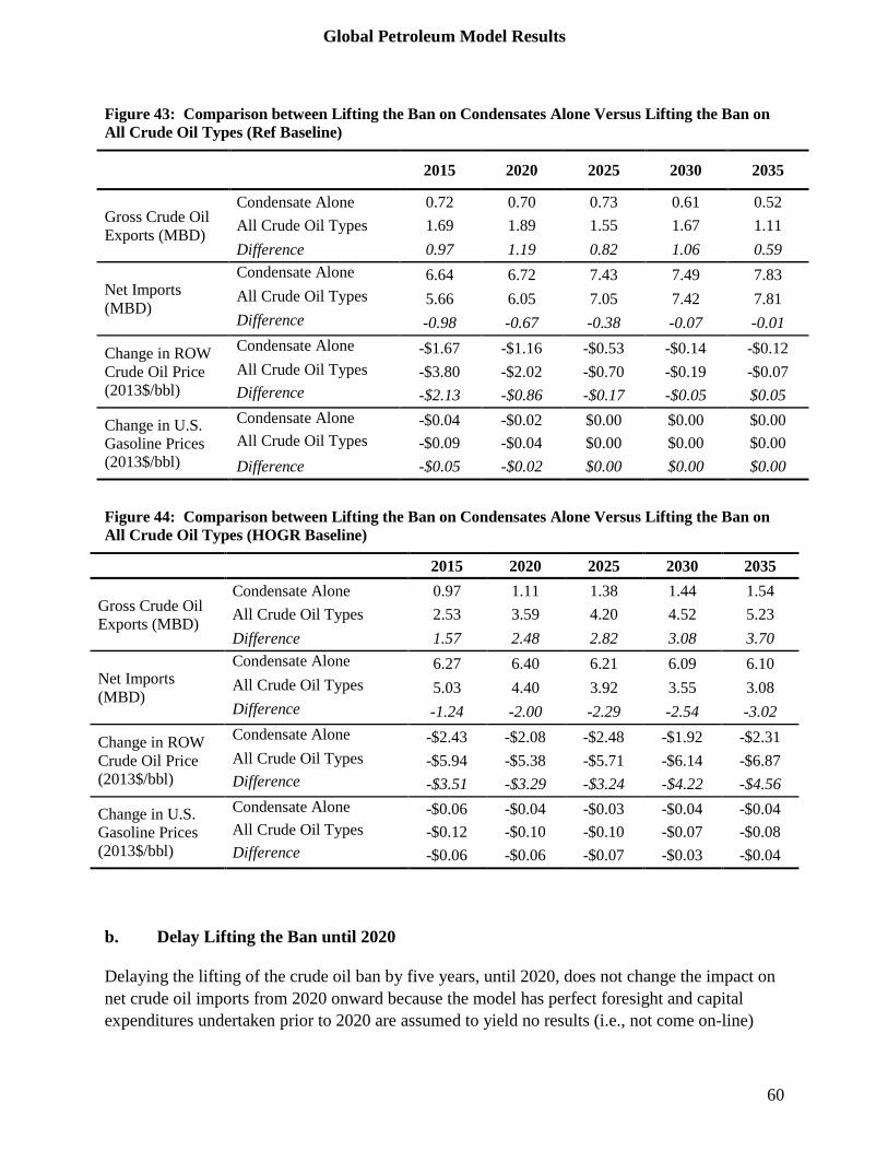
Global Petroleum Model Results
60
Figure 43: Comparison between Lifting the Ban on Condensates Alone Versus Lifting the Ban on All Crude Oil Types (Ref Baseline)
2015 2020 2025 2030 2035
Gross Crude Oil Exports (MBD)
Condensate Alone 0.72 0.70 0.73 0.61 0.52 All Crude Oil Types 1.69 1.89 1.55 1.67 1.11 Difference 0.97 1.19 0.82 1.06 0.59
Net Imports (MBD)
Condensate Alone 6.64 6.72 7.43 7.49 7.83 All Crude Oil Types 5.66 6.05 7.05 7.42 7.81 Difference -0.98 -0.67 -0.38 -0.07 -0.01
Change in ROW Crude Oil Price (2013$/bbl)
Condensate Alone -$1.67 -$1.16 -$0.53 -$0.14 -$0.12 All Crude Oil Types -$3.80 -$2.02 -$0.70 -$0.19 -$0.07 Difference -$2.13 -$0.86 -$0.17 -$0.05 $0.05
Change in U.S. Gasoline Prices (2013$/bbl)
Condensate Alone -$0.04 -$0.02 $0.00 $0.00 $0.00 All Crude Oil Types -$0.09 -$0.04 $0.00 $0.00 $0.00 Difference -$0.05 -$0.02 $0.00 $0.00 $0.00
Figure 44: Comparison between Lifting the Ban on Condensates Alone Versus Lifting the Ban on All Crude Oil Types (HOGR Baseline)
2015 2020 2025 2030 2035
Gross Crude Oil Exports (MBD)
Condensate Alone 0.97 1.11 1.38 1.44 1.54 All Crude Oil Types 2.53 3.59 4.20 4.52 5.23 Difference 1.57 2.48 2.82 3.08 3.70
Net Imports (MBD)
Condensate Alone 6.27 6.40 6.21 6.09 6.10 All Crude Oil Types 5.03 4.40 3.92 3.55 3.08 Difference -1.24 -2.00 -2.29 -2.54 -3.02
Change in ROW Crude Oil Price (2013$/bbl)
Condensate Alone -$2.43 -$2.08 -$2.48 -$1.92 -$2.31 All Crude Oil Types -$5.94 -$5.38 -$5.71 -$6.14 -$6.87 Difference -$3.51 -$3.29 -$3.24 -$4.22 -$4.56
Change in U.S. Gasoline Prices (2013$/bbl)
Condensate Alone -$0.06 -$0.04 -$0.03 -$0.04 -$0.04 All Crude Oil Types -$0.12 -$0.10 -$0.10 -$0.07 -$0.08 Difference -$0.06 -$0.06 -$0.07 -$0.03 -$0.04
b. Delay Lifting the Ban until 2020
Delaying the lifting of the crude oil ban by five years, until 2020, does not change the impact on net crude oil imports from 2020 onward because the model has perfect foresight and capital expenditures undertaken prior to 2020 are assumed to yield no results (i.e., not come on-line)

Global Petroleum Model Results
61
until 2020 or later. In other words, there are no useful ways in the model for refiners to spend money in 2015 to change their refinery configurations prior to 2020. Thus, investment decisions remain the same whether the ban is lifted in 2015 or 2020 because in both cases the U.S. has no export ban in 2020. Other parameters discussed above are similarly unaffected. A delay in lifting of the crude oil export ban does mean that during the period of the delay the economic benefits resulting from lifting of the ban are foregone.
Figure 45 and Figure 45 compare the impacts for the case in which the ban is lifted in 2015 to delaying the lifting to 2020.
Figure 45: Net Crude Oil Imports Resulting from the Complete Lifting of the Crude Oil Export Ban in 2015 and 2020 (Ref Baseline: MBD)
2015 2020 2025 2030 2035
Net Crude Oil Imports (MBD)
Ban Lifted in 2015 5.7 6.0 7.1 7.4 7.8 Ban Lifted in 2020 7.3 6.0 7.1 7.4 7.8 Difference 1.6 0.0 0.0 0.0 0.0
Figure 46: Net Crude Oil Imports Resulting from the Complete Lifting of the Ban in 2015 and 2020 (HOGR Baseline: MBD
2015 2020 2025 2030 2035
Net Crude Oil Imports (MBD)
Ban Lifted in 2015 5.0 4.4 3.9 3.5 3.1 Ban Lifted in 2020 7.2 4.4 3.9 3.5 3.1 Difference 2.1 0.0 0.0 0.0 0.0

Macroeconomic Impacts
62
V. MACROECONOMIC IMPACTS
Any policy change that has implications for international trade, such as lifting of the crude oil exports ban, will have effects throughout the economy over and above its direct effects on U.S. energy prices, supply and demand. The immediate consequence of lifting the ban would be increased export earnings that would exceed the cost of producing the crude oil being exported. In addition, lifting of the ban would remove distortions similar to those created by price controls and bring efficiency to U.S. refinery operations. The U.S. economy would also benefit from lower world crude oil prices. Everything else being equal, including the amount of borrowing by the United States from foreign sources, lifting of the ban will cause the value of the dollar to increase. The increase in the value of the dollar and the increase in U.S. crude oil prices that accompanies the expansion of crude oil exports will raise the cost of other exports to foreign customers, leading to a shift in the composition of exports. In addition, the dollar price of goods imported into and consumed in the United States will fall, leading to an increase in imports that balances the net increase in exports. These changes will in turn affect wage rates, change returns on capital, spur investment in different industries, and lower the prices of goods and services purchased by consumers.
A. U.S. Consumer Wellbeing (Welfare)
The broadest measure of net economic benefits to U.S. residents is the measure of economic welfare known as the “equivalent variation.” The equivalent variation is defined as the amount of money that would have to be given to U.S. households to make them indifferent between receiving the money and experiencing the changes in prices and income associated with lifting the ban.32 The more money it takes to provide an equal benefit to that conferred by lifting the crude oil exports ban, the larger the benefits of exports must be.
We report the change in welfare relative to the same baseline in which the ban is in effect for all the scenarios so that the U. S. resource and global oil demand assumptions are consistent between the scenario and the baseline. Thus the Ref scenarios are measured against the Ref baseline, HOGR scenarios are measured against the HOGR baseline and LowAP scenario impacts are measured against the corresponding LowAP baseline. A positive change in welfare means that the policy improves welfare from the perspective of the consumer. As discussed below, all scenarios are welfare-improving for U.S. consumers.
32 Intermediate Microeconomics: A Modern Approach, Hal Varian, 7th Edition (December 2005), W.W. Norton &
Company, pp. 255-256. “Another way to measure the impact of a price change in monetary terms is to ask how much money would have to be taken away from the consumer before the price change to leave him as well off as he would be after the price change. This is called the equivalent variation in income since it is the income change that is equivalent to the price change in terms of the change in utility.” (emphasis in original).

Macroeconomic Impacts
63
1. Immediate lifting of the ban is beneficial to the U.S. consumers:
Under the Ref case, lifting of the ban improves welfare by about 0.28% in 2015, an improvement that decreases to less than 0.1% by 2035, shown in Figure 47. Overall, welfare improves by about 0.13%. Under the HOGR case, welfare improvement is about 0.62% in 2015 and declines to about 0.41% by the end of the model horizon. Under the HOGR crude oil exports continue to increase over the model horizon unlike the Ref case. Hence benefits to the U.S. consumers are sustained over the model horizon resulting in slower decline in welfare. Also, gains from crude oil exports are much larger for the U.S. under HOGR due to an abundant crude oil outlook and lower domestic costs of production. Consumer benefit is about three times larger under the HOGR than under the Ref case.
Figure 47: Change in Welfare Resulting from the Complete Lifting of the Ban in 2015 (Ref and HOGR Baselines: %)
2. Delaying the lifting of the ban reduces net benefit:
Figure 48 shows percentage change in welfare from lifting the ban immediately and delaying it till 2020 for the Ref and the HOGR cases. In all cases the welfare increases suggesting there are benefits to the U.S. consumers even if there is a delay in lifting the ban. In terms of net present value of welfare, under the delay scenarios, welfare improves by about 0.05% and 0.30% in the Ref and the HOGR cases, respectively.
0.00
0.10
0.20
0.30
0.40
0.50
0.60
0.70
2015 2020 2025 2030 2035 DNPV
% C
hang
e
Ref HOGR

Macroeconomic Impacts
64
Under the Ref case, delaying the ban till 2020 provides very little benefit in 2015. This is expected since there is no crude oil export in 2015. Moreover, under the Ref case a large part of the benefit is accrued in the first fifteen years since exports are very small in the out years (post 2025). Thus in the Ref case delaying the ban foregoes the opportunity to capture a large share of the benefits of freeing crude oil exports, and welfare gains are only 30% of the improvement possible if the ban is lifted immediately. This foregone benefit is primarily due to skipping the benefit in 2015 which accounts for about 50% of the overall benefit.
Figure 48: Change in Welfare Resulting from the Complete Lifting of the Ban in 2015 and 2020 (Ref and HOGR Baselines: %)
Under the HOGR scenarios, lifting the ban in 2020 rather than 2015 results in smaller welfare gains relative to lifting the ban immediately. In HOGR, the 2015 benefits are not as large a share of the overall welfare improvement, and therefore, the foregone benefits due to delay are proportionally smaller than in the Ref case. Welfare improvement under the HOGR delay scenario is about 70% of lifting of the ban immediately (see the last four columns of Figure 48).
Thus the delay scenario still provides net benefits to the U.S. consumers in both the Ref and HOGR cases, but it is gives much smaller gains in the Ref case than in the HOGR case. Delaying the lifting of the ban misses out on the opportunity to capture the net benefits of exports in 2015, when they are largest in the Ref case but about average of exports over the 2015-2035 time period in the HOGR case.
3. Partial lifting of the ban provides smaller benefit:
As with the delaying the lifting of the ban, partial lifting of the ban by allowing only exports of condensate also provides smaller net benefits. Figure 49 below shows welfare changes for lifting of the ban completely and partial lifting of the ban for years 2015, 2025, and 2035. The figure also shows overall welfare impacts, labeled as DPNV. The overall welfare improvement under this partial lifting of the ban is 0.05% and 0.12% for the Ref and the HOGR cases, respectively. This is because allowing condensate only, the benefits are limited to smaller export volumes and the price feedback benefits from the rest of the world are also limited. The welfare improvement
0.00
0.10
0.20
0.30
0.40
0.50
0.60
0.70
2015 2025 2035 DNPV
% C
hang
e
NoBan NoBanDelay2015 2025 2035 DNPV
NoBan NoBanDelay

Macroeconomic Impacts
65
under partial lifting is about one-third of lifting the ban immediately for the Ref case. However, net benefits under the HOGR case are even smaller in relative terms (one-fourth of those from lifting the ban immediately) since condensate exports are a smaller share of the total crude oil exports under the HOGR case compared to the Ref case. Hence, condensate exports provide relatively smaller benefits under the HOGR case than under the Ref case. Our analysis shows that although exporting condensate benefits the U.S., benefits could be increased greatly by lifting the ban completely.
Figure 49: Change in Welfare Resulting from the Complete Lifting of the Ban in 2015 and Lifting of the Ban on Condensates (Ref and HOGR Baselines: %)
4. Change in OPEC responses does not alter net benefits to the U.S. economy:
The U.S. exports the same amount of crude oil under the OPECFix case and immediate lifting of the ban case. Under the OPECCut cases, U.S. exports volumes are at their highest. Under the HOGR OPECCut case, U.S. exports about 0.5 MBD more of crude oil than under the OPECFix case. Similarly, under the Ref OPECCut case, U.S. exports about 0.25 MBD more in the short run than under the OPECFix case.
The combination of gains from crude oil exports and benefits associated with the large drop in the world crude oil price make the welfare benefits for the OPECFix cases similar to the cases where OPEC is a normal market participant. This is true in both the Ref and the HOGR cases as shown in Figure 50. However, under the OPECCut cases, the gains from crude oil exports are tempered by relatively smaller import benefits, since the world crude oil price remains at higher levels under the OPECCut cases. As a result of these effects, the welfare increase in the OPECCut cases are much smaller than under the OPECFix cases. Under the Ref and the HOGR cases, OPECCut welfare improves by about 0.10% and 0.30%, respectively. While for the OPECFix cases, welfare improvements are about 0.20% and 0.50%, respectively because the U.S. enjoys more favorable terms of trade.
0.00
0.10
0.20
0.30
0.40
0.50
0.60
0.70
2015 2025 2035 DNPV
% C
hang
e
NoBan NoBanCond2015 2025 2035 DNPV
NoBan NoBanCond

Macroeconomic Impacts
66
Figure 50: Change in Welfare Resulting from the Complete Lifting of the Ban in 2015 under Different OPEC Responses (Ref and HOGR Baselines: %)
The U.S. exports the same amount of crude oil under the OPECFix case and immediate lifting of the ban case. Under the OPECCut cases, U.S. exports volumes are at their highest. Under the HOGR OPECCut case, U.S. exports about 0.5 MBD more of crude oil than under the OPECFix case. Similarly, under the Ref OPECCut case, U.S. exports about 0.25 MBD more in the short run than under the OPECFix case.
The combination of gains from crude oil exports and benefits associated with the large drop in the world crude oil price make the welfare benefits for the OPECFix cases similar to the cases where OPEC is a normal market participant. This is true in both the Ref and the HOGR cases as shown in Figure 50. However, under the OPECCut cases, the gains from crude oil exports are tempered by relatively smaller import benefits, since the world crude oil price remains at higher levels under the OPECCut cases. As a result of these effects, the welfare increase in the OPECCut cases are much smaller than under the OPECFix cases. Under the Ref and the HOGR cases, OPECCut welfare improves by about 0.10% and 0.30%, respectively. While for the OPECFix cases, welfare improvements are about 0.20% and 0.50%, respectively because the U.S. enjoys more favorable terms of trade.
5. With lower world oil demand, the U.S. economy still benefits from exporting crude oil:33
Under the lower Asia Pacific demand scenario crude oil exports are 0.5 MBD lower in the long run and fairly similar in the short run for the HOGR case. The crude oil export volumes under the Ref case are fairly similar. The U.S. has a larger impact on the world crude oil price under this market condition because the U.S. exports are a larger percentage increase in a smaller total
33 Given the similarities between the macroeconomic impacts between lifting the ban completely and the low Asia
Pacific scenario, from here on out we will not discuss the results for this scenario. Details on the impacts for this scenario can be found in the Appendices.
0.00
0.10
0.20
0.30
0.40
0.50
0.60
0.70
2015 2025 2035 DNPV
% C
hang
e
NoBan NoBanFix NoBanCut2015 2025 2035 DNPV
NoBan NoBanFix NoBanCut

Macroeconomic Impacts
67
world supply. Lower crude oil exports and larger price drop add up to similar impacts on the U.S. compared to the lifting of the ban completely, as shown in Figure 51.
Figure 51: Change in Welfare Resulting from the Complete Lifting of the Ban in 2015 under Different Assumptions about Asia Pacific Demand for Refined Petroleum Products (Ref and HOGR Baselines: %)
6. Summary: Immediate lifting of the ban on all crude oil exports results in the greatest economic benefits for the U.S.:
Figure 52 below summarizes the net benefit to the U.S. consumers across all sectors. The U.S. net benefits under the HOGR are about two to six times greater than under the Ref cases. Under the Ref cases, welfare improvement for the partial or the delayed scenarios is about 40% smaller than lifting the ban completely. Under the HOGR, partial lifting of the ban provides the smallest benefit, 27% of lifting the ban completely. Different market condition and OPEC responses still allows the U.S. to reap net benefits from lifting the ban.
0.00
0.10
0.20
0.30
0.40
0.50
0.60
0.70
2015 2025 2035 DNPV
% C
hang
e
NoBan NoBanLowAP2015 2025 2035 DNPV
NoBan NoBanLowAP

Macroeconomic Impacts
68
Figure 52: Change in Net Present Value of Welfare Resulting from Complete and Modified Lifting of the Ban under Different Assumptions about OPEC’s Response (Ref and HOGR Baselines: %)
B. Aggregate consumption
Aggregate consumption measures total spending on goods and services in the economy. Higher aggregate spending or consumption resulting from a policy suggests higher economic activity and more purchasing power for consumers.
Aggregate consumption, under the NoBan scenario, increases by about 0.29% and 0.63% for the Ref and the HOGR in 2015, respectively, when the export ban on all crude oils is lifted immediately (see Figure 53). These income increases for the consumers amount to about $35 billion and $78 billion. Under the HOGR case, the increase in consumption is sustained between $78 to $81 billion over the model horizon as a result of continued net gain in crude oil exports and lower world oil prices. However, smaller aggregate consumption gains are realized in the Ref case because the crude oil export gains are not as large for the U.S. resulting in consumption increases that are smaller by 2035. In the Ref case, aggregate consumption increases by about $20 billion in 2035 (see Figure 54). These consumption increases are about 0.5% and 1.1% of a typical U.S. median household income.34
34 According to U.S. Census Bureau median household income between 2008 through 2012 was about $53,000.
0.00
0.05
0.10
0.15
0.20
0.25
0.30
0.35
0.40
0.45
0.50%
Cha
nge
NoBan NoBanDelay NoBanCondNoBanOPECFix NoBanOPECCut NoBanLowAP
Ref HOGR
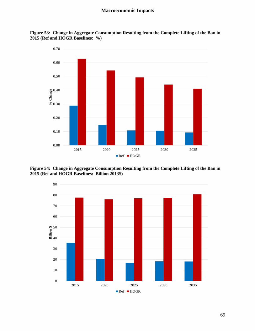
Macroeconomic Impacts
69
Figure 53: Change in Aggregate Consumption Resulting from the Complete Lifting of the Ban in 2015 (Ref and HOGR Baselines: %)
Figure 54: Change in Aggregate Consumption Resulting from the Complete Lifting of the Ban in 2015 (Ref and HOGR Baselines: Billion 2013$)
0.00
0.10
0.20
0.30
0.40
0.50
0.60
0.70
2015 2020 2025 2030 2035
% C
hang
e
Ref HOGR
0
10
20
30
40
50
60
70
80
90
2015 2020 2025 2030 2035
Bill
ion
$
Ref HOGR

Macroeconomic Impacts
70
Assuming 133 million household units in 201335, an average U.S. household will experience an income increase of $270 in the Ref case and $590 in the HOGR case in 2015 as a result of lifting the crude oil export ban. Figure 55 shows increase in per household for all scenarios. Delaying and the partial lifting of the crude oil export ban result in the smallest increase in income per household.
Figure 55: Change in 2015 Income per Household Resulting from the Complete and Partial Lifting of the Ban under Different OPEC Responses (Ref and HOGR Baselines: 2013$ per Household)
Similar to the welfare impacts, aggregate consumption benefits are mostly eliminated in 2015 if the lifting of the ban is delayed until 2020. U.S. household consumption in the delay scenarios is about $4.8 billion for the Ref case and $33 billion in the HOGR case. The loss is consumption benefit from delaying the lifting of the ban is about $31 billion and $45 billion in 2015 under the Ref and the HOGR cases, respectively. Figure 56 below shows the change in aggregate consumption by lifting the ban immediately and delaying the lifting of the ban.
35Census Bureau http://quickfacts.census.gov/qfd/states/00000.html
$0
$100
$200
$300
$400
$500
$600
$700
Ref HOGR
$ pe
r H
ouse
hold
NoBan NoBanDelay NoBanCond NoBanOPECFix NoBanOPECCut

Macroeconomic Impacts
71
Figure 56: Change in Aggregate Consumption Resulting from the Complete Lifting of the Ban in 2015 and 2020 (Ref and HOGR Baselines: Billion 2013$)
Aggregate consumption increases in all scenarios. Over the next 25 years, 2015 through 2039, change in the net present value of aggregate consumption for the 5 scenarios (NoBan, NoBanDelay, NoBanCond, NoBanOPECFix, and NoBanOPECCut) are shown in Figure 57. Under the Ref case cumulative net present value of consumption increases are about $390, $140, $150, $410, and $210 billion, respectively. For the same HOGR scenarios, cumulative net present value increases are about $1,260, $870, $370, $1,290, and $770 billion, respectively. The smallest increases in consumption among the HOGR cases are found in the scenario with partial lifting of the ban and in the scenario in which OPEC responds by reducing output, while in the Ref cases, the scenarios with partial lifting and with delays in lifting the ban yield the smallest gains.
$0
$10
$20
$30
$40
$50
$60
$70
$80
$90
2015 2020 2025 2030 2035
Bill
ion
$
NoBan NoBanDelay2015 2020 2025 2030 2035
NoBan NoBanDelay

Macroeconomic Impacts
72
Figure 57: Change in Cumulative Net Present Value of Aggregate Consumption between 2015 through 2039 Resulting from the Complete and Partial Lifting of the Ban under Different OPEC Responses (Ref and HOGR Baselines: Billion 2013$)
C. Investment
Investment in the economy occurs to replace old capital and augment new capital formation. Since personal income must be allocated to one of these choices, in any given year investment comes at the expense of consumption and vice versa. When the ban is lifted, additional investment takes place to expand the crude oil extraction sector. The industrial and manufacturing sectors also require some additional capital demand to support higher investment in the crude oil sector. The extent of the increase in investment depends upon the crude oil sector expansion or crude oil exports. Additional investment occurs throughout the model horizon in the HOGR cases; while additional investment in the Ref cases occurs primarily in the first model year.
$0
$200
$400
$600
$800
$1,000
$1,200
$1,400
Ref HOGR
Bill
ion
$
NoBan NoBanDelay NoBanCond NoBanOPECFix NoBanOPECCut
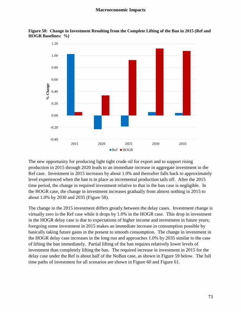
Macroeconomic Impacts
73
Figure 58: Change in Investment Resulting from the Complete Lifting of the Ban in 2015 (Ref and HOGR Baselines: %)
The new opportunity for producing light tight crude oil for export and to support rising production in 2015 through 2020 leads to an immediate increase in aggregate investment in the Ref case. Investment in 2015 increases by about 1.0% and thereafter falls back to approximately level experienced when the ban is in place as incremental production tails off. After the 2015 time period, the change in required investment relative to that in the ban case is negligible. In the HOGR case, the change in investment increases gradually from almost nothing in 2015 to about 1.0% by 2030 and 2035 (Figure 58).
The change in the 2015 investment differs greatly between the delay cases. Investment change is virtually zero in the Ref case while it drops by 1.0% in the HOGR case. This drop in investment in the HOGR delay case is due to expectations of higher income and investment in future years; foregoing some investment in 2015 makes an immediate increase in consumption possible by basically taking future gains in the present to smooth consumption. The change in investment in the HOGR delay case increases in the long run and approaches 1.0% by 2035 similar to the case of lifting the ban immediately. Partial lifting of the ban requires relatively lower levels of investment than completely lifting the ban. The required increase in investment in 2015 for the delay case under the Ref is about half of the NoBan case, as shown in Figure 59 below. The full time paths of investment for all scenarios are shown in Figure 60 and Figure 61.
-0.40
-0.20
0.00
0.20
0.40
0.60
0.80
1.00
1.20
2015 2020 2025 2030 2035
% C
hang
e
Ref HOGR

Macroeconomic Impacts
74
Figure 59: Percentage Change in 2015 Investment Resulting from the Complete and Partial Lifting of the Ban (Ref and HOGR Baselines: %)
Figure 60: Change in Investment Resulting from a Lifting of the Ban under Different Assumptions about OPEC’s Response (Ref Baseline: %)
-1.50
-1.00
-0.50
0.00
0.50
1.00
1.50
Ref HOGR
% C
hang
e
NoBan NoBanDelay NoBanCond
-0.40
-0.20
0.00
0.20
0.40
0.60
0.80
1.00
1.20
2015 2020 2025 2030 2035
% C
hang
e
NoBan NoBanDelay NoBanCond NoBanOPECFix NoBanOPECCut

Macroeconomic Impacts
75
Figure 61: Change in Investment Resulting from a Lifting of the Ban under Different Assumptions about OPEC’s Response (HOGR Baseline: %)
D. Gross Domestic Product
Gross Domestic Product (GDP) measures the total economic activity in the economy and is another metric used to evaluate the effectiveness of a policy. GDP impacts are positive if the economy expands leading to higher income from different income sources to consumers. Income sources could be in the form of labor, capital, or resource income. GDP could also be impacted by higher levels of investment or gains in the current account balance to the economy.
-1.50
-1.00
-0.50
0.00
0.50
1.00
1.50
2015 2020 2025 2030 2035
% C
hang
e
NoBan NoBanDelay NoBanCond NoBanOPECFix NoBanOPECCut

Macroeconomic Impacts
76
Figure 62: Change in GDP Resulting from the Complete Lifting of the Ban in 2015 (Ref and HOGR Baselines: %)
By lifting the ban under the Ref case, the GDP increase in 2015 is about 0.40% and then diminishes rapidly over time. The GDP impact by 2035 is almost zero in this case (see Figure 62). However, in the HOGR case, the GDP increase in 2015 is about 0.58% and exceeds 0.70% by 2035. Under the HOGR case, increasing crude oil exports over time maintains a positive and high level of GDP impacts over time. GDP impacts for the Ref are primarily front loaded similar to other impacts that have been discussed in the prior sections.
In the Ref and HOGR cases, the average annual GDP increase is between $4.0 to $66 billion, and $80 to $180 billion, respectively (Figure 63).
Immediately lifting the ban on crude oil exports results in higher levels of GDP over the entire model horizon. The high level of GDP impacts under the HOGR mirrors the high level of consumption and investment over the model horizon.
0.00
0.10
0.20
0.30
0.40
0.50
0.60
0.70
0.80
2015 2020 2025 2030 2035
% C
hang
e
Ref HOGR

Macroeconomic Impacts
77
Figure 63: Change in GDP Resulting from the Complete Lifting of the Ban in 2015 (Ref and HOGR Baselines: Billion 2013$)
In both cases, partial lifting of the ban has the smallest GDP benefit, while other scenarios span the range of GDP impact shown in
Figure 64. The range of GDP impacts is much smaller and front loaded for the Ref case because the gains from crude oil exports are limited to the first three model years. However, for the HOGR scenarios the range is much larger. By 2035, GDP change ranges from $50 billion for the condensate export only case to about $200 billion under the most favorable case of completely lifting the ban immediately.
0
50
100
150
200
250
2015 2020 2025 2030 2035
Bill
ion
$
Ref HOGR

Macroeconomic Impacts
78
Figure 64: Range of Change in U.S. GDP Resulting from the Partial or Complete Lifting of the Crude Oil Export Ban (Ref and HOGR Baselines: Billion 2013$)
Under the Ref case, the change in the net present value (NPV) of GDP ranges from $230 to $580 billion; while for the HOGR case, it ranges from $590 to $1,800 billion (Figure 65). If future crude oil supplies are close to those forecasted in the HOGR case, just allowing exports of condensate in the HOGR case could yield similar benefits to lifting the ban on all crudes if resources proved closer to those in the Ref case. As shown with other indicators, delaying the export ban is relatively less harmful in the HOGR than in the Ref case because in the HOGR case, it does not mean losing about half the increment to total production in the first year.
-50
0
50
100
150
200
250
2015 2020 2025 2030 2035 2015 2020 2025 2030 2035
Ref HOGR
Bill
ion
$

Macroeconomic Impacts
79
Figure 65: Range of Change in U.S. Net Present Value of GDP Resulting from the Partial or Complete Lifting of the Crude Oil Export Ban (Ref and HOGR Baselines: Billion 2013$)
To understand the GDP impacts better, we decompose the individual components of GDP from the income sources: wage income, capital income, resource and sector-specific capital, and indirect tax revenues. Investment translates directly into changes in input levels for a given sector. In general, as a result of investment stimulus, if the output of a sector increases, so do the inputs associated with the production of this sector’s goods and services. An increase in crude oil output also leads to more wage income in the crude oil sector as domestic production increases. In the short run, industries are able to adjust to changes in demand for output by increasing employment if the sector expands or by reducing employment if the sector contracts. The overall macroeconomic impacts are driven by the changes in the sources of household income. Figure 66, Figure 67, and Figure 68 below show changes in the income sources for the Ref and HOGR cases.
In the Ref case, higher demand for intermediate goods and services as a result from higher investment leads to an increase in demand for labor and capital. In addition, higher crude oil production leads to an increase in labor demand as well as resource and sector-specific capital. These effects translate into an increase in labor income in the short run, mainly in 2015. Beyond 2015 for the Ref case, increases in GDP result from resource and sector-specific capital only as demand for intermediate goods and services declines. Figure 67 shows that there is no change after 2015 in incomes outside the crude oil sector; but there is continuing return to resource and specialized capital in the crude oil sector as production continues from the initial capital investment.
0
200
400
600
800
1000
1200
1400
1600
1800
2000
Ref HOGR
Ran
ge o
f Cha
nge
in G
DP
(Bill
ion
$)

Macroeconomic Impacts
80
Figure 66: Shift in Income Sources in 2015 Resulting from a Partial and Complete Lifting of the Ban under Different Assumptions about OPEC’s Response (Ref Baseline: Billion 2013$)
-10
0
10
20
30
40
50
60
70
NoBan NoBanDelay NoBanCond NoBanOPECFix NoBanOPECCut
Bill
ion
$
Wage Income Capital Income Resource & Sector Specific Capital Income Indirect Tax Revenues

Macroeconomic Impacts
81
Figure 67: Shift in Income Sources in 2015, 2025, and 2035 Resulting from a Partial and Complete Lifting of the Ban under Different Assumptions about OPEC’s Response (Ref Baseline: Billion 2013$)
In the HOGR cases, all income sources improve. Both wage and capital income increases as demand for intermediate goods and services increases. Resource and specialized capital income also grows over time and is higher in the later years as a result of higher export, but labor income remains higher.
-20
-10
0
10
20
30
40
50
60
70
80N
oBan
NoB
anD
elay
NoB
anC
ond
NoB
anO
PEC
Fix
NoB
anO
PEC
Cut
NoB
an
NoB
anD
elay
NoB
anC
ond
NoB
anO
PEC
Fix
NoB
anO
PEC
Cut
NoB
an
NoB
anD
elay
NoB
anC
ond
NoB
anO
PEC
Fix
NoB
anO
PEC
Cut
2015 2025 2035
Bill
ion
$
Wage Income Capital Income Resource & Sector Specific Capital Income Indirect Tax Revenues

Macroeconomic Impacts
82
Figure 68: Shift in Income Sources in 2015, 2025, and 2035 Resulting from a Partial and Complete Lifting of the Ban under Different Assumptions about OPEC’s Response (HOGR Baseline: Billion 2013$)
E. Impact on Labor Markets
Removing the oil export ban would have a universally positive effect on labor markets. Labor income increases in all scenarios during the period when exports lead to increased domestic oil production. Increased demand for labor for oil exploration and production and a lower cost of living due to reduced prices of refined petroleum products cause higher real wages. And the stimulus of added investment in oil and gas drilling during the period while the economy is still recovering from the recession causes a more rapid return to full employment.
1. Change in labor income
Figure 69 shows the increase in annual labor income in billions of 2013 dollars. Whether tight crude oil resources turn out to be at the Ref or the High Oil and Gas Resource levels, removing the ban on exports lead to an immediate increase in exploration and production activity and a corresponding immediate increase in labor income. The increases in labor income lead the pattern of increases in crude oil production (see Figure 1) because drilling activity must increase before production can begin to rise. As production increases become smaller in 2020 and later, the increase in labor income shrinks as well. By 2035 in the Ref Case, production and labor income are the same with or without the ban.
-50
0
50
100
150
200
250N
oBan
NoB
anD
elay
NoB
anC
ond
NoB
anO
PEC
Fix
NoB
anO
PEC
Cut
NoB
an
NoB
anD
elay
NoB
anC
ond
NoB
anO
PEC
Fix
NoB
anO
PEC
Cut
NoB
an
NoB
anD
elay
NoB
anC
ond
NoB
anO
PEC
Fix
NoB
anO
PEC
Cut
2015 2025 2035
Bill
ion
$
Wage Income Capital Income Resource & Sector Specific Capital Income Indirect Tax Revenues
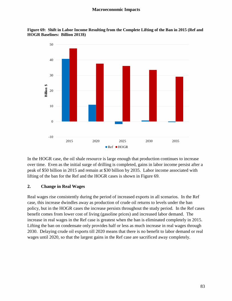
Macroeconomic Impacts
83
Figure 69: Shift in Labor Income Resulting from the Complete Lifting of the Ban in 2015 (Ref and HOGR Baselines: Billion 2013$)
In the HOGR case, the oil shale resource is large enough that production continues to increase over time. Even as the initial surge of drilling is completed, gains in labor income persist after a peak of $50 billion in 2015 and remain at $30 billion by 2035. Labor income associated with lifting of the ban for the Ref and the HOGR cases is shown in Figure 69.
2. Change in Real Wages
Real wages rise consistently during the period of increased exports in all scenarios. In the Ref case, this increase dwindles away as production of crude oil returns to levels under the ban policy, but in the HOGR cases the increase persists throughout the study period. In the Ref cases benefit comes from lower cost of living (gasoline prices) and increased labor demand. The increase in real wages in the Ref case is greatest when the ban is eliminated completely in 2015. Lifting the ban on condensate only provides half or less as much increase in real wages through 2030. Delaying crude oil exports till 2020 means that there is no benefit to labor demand or real wages until 2020, so that the largest gains in the Ref case are sacrificed away completely.
-10
0
10
20
30
40
50
2015 2020 2025 2030 2035
Bill
ion
$
Ref HOGR

Macroeconomic Impacts
84
Figure 70: Change in Real Wage Resulting from a Lifting of the Ban under Different Assumptions about OPEC’s Response (Ref Baseline: %)
The increase in real wages is also more modest if OPEC were to cut production sufficiently to prevent reductions in world oil prices. In this case, the reduction in the cost of living that contributes to increased real wages disappears, so that only the benefits of higher labor demand on real wages remain.
-0.10
0.00
0.10
0.20
0.30
0.40
0.50
0.60
2015 2020 2025 2030 2035
% C
hang
e
NoBan NoBanDelay NoBanCond NoBanOPECFix NoBanOPECCut

Macroeconomic Impacts
85
Figure 71: Change in Real Wage Resulting from a Lifting of the Ban under Different Assumptions about OPEC’s Response (HOGR Baseline: %)
In the HOGR case, all the beneficial impacts on real wages are larger and sustained. The differences in impacts across the three policy scenarios and the sensitivity case for OPEC mirror those in the Ref case, with the exception of the effect of delay. In the HOGR case, there are still two decades of increased production even if the ban is not removed until 2020, but the foregone benefits in 2015 are also much larger. The effects of removing the condensate ban only also fall shorter of the benefits of full removal in the HOGR case, because condensate is a smaller share of increased production in the HOGR case.
-0.10
0.00
0.10
0.20
0.30
0.40
0.50
0.60
0.70
2015 2020 2025 2030 2035
% C
hang
e
NoBan NoBanDelay NoBanCond NoBanOPECFix NoBanOPECCut

Macroeconomic Impacts
86
Figure 72: Change in 2015 Real Wage from Lifting the Ban (Ref and HOGR Baselines: %)
Figure 73: Change in 2015 and 2035 Real Wage from Lifting the Ban (Ref and HOGR Baselines: %)

Macroeconomic Impacts
87
F. Reduction in Unemployment
As a long-term model of economic growth, NewERA does not address issues of business cycles and unemployment, assuming instead that real and potential GDP coincide and that labor markets are in equilibrium like all other markets. As the U.S. economy is still recovering slowly from the recession, it is likely that policies toward crude oil exports could affect the speed at which the recovery progresses.
1. Transitional Unemployment
The NewERA model assumes full employment in the U.S. economy over the long time horizon covered by the model. This assumption is consistent with the long-term performance of the U.S. economy, which has generally operated at full employment since the Second World War, and recognizes the impossibility of predicting the timing or depth of future downturns. CBO’s baseline forecast has the economy returning to full employment in 2018, and states: “For the second half of the coming decade, CBO does not attempt to predict the cyclical ups and downs of the economy; rather, CBO assumes that GDP will stay at its maximum sustainable level.”36
The assumption of full employment does not imply that the measured unemployment rate will be zero. CBO’s estimate of the natural (or equilibrium) rate of unemployment that corresponds to “full employment” is “the ‘nonaccelerating inflation rate of unemployment’ (NAIRU), which is the rate of unemployment consistent with a stable rate of inflation.”37 CBO estimates the NAIRU using the historical relationship between the unemployment rate and changes in the rate of inflation. This level of unemployment is also referred to as the “natural rate.” The natural rate is not zero because of frictions in the labor market, which include time spent on job searches when workers move from one job to another; structural factors, including disincentives for work such as long-term unemployment compensation and income-tested transfer payment; and mismatches between skills and labor demand, especially in the presence of minimum wage laws that make it uneconomic to fill jobs with low productivity.
“Potential” GDP is another important concept that influences unemployment. Potential GDP is based on the productive potential of the economy, which grows over time with capital investment, productivity improvement, and resource discoveries. When actual GDP equals potential GDP, unemployment will be at the natural rate.
CBO projects that the unemployment rate will remain above the NAIRU until 2018 as the economy recovers slowly from the recession:
36 CBO, “The Budget and Economic Outlook: Fiscal Years 2013 to 2023," February 5, 2013. 37 Robert Arnold, “REESTIMATING THE PHILLIPS CURVE AND THE NAIRU,” Congressional Budget Office,
Washington, DC, August 2008, pg. 3.

Macroeconomic Impacts
88
… underlying economic factors will lead to more rapid growth, CBO projects—3.4 percent in 2014 and an average of 3.6 percent a year from 2015 through 2018. In particular, CBO expects that the effects of the housing and financial crisis will continue to fade and that an upswing in housing construction (though from a very low level), rising real estate and stock prices, and increasing availability of credit will help to spur a virtuous cycle of faster growth in employment, income, consumer spending, and business investment over the next few years.
Nevertheless, under current law, CBO expects the unemployment rate to remain high—above 7½ percent through 2014—before falling to 5½ percent at the end of 2017.38
Figure 74: Historical and CBO Projected Unemployment Rates (%)39
2013 2014 2015 2016 2017 2018 Unemployment Rate, Civilian, 16 Years or Older 7.9 7.8 7.1 6.3 5.6 5.5
Since 2015 is the first year reported in our study, our assumptions for the years from 2018 onwards -- that the economy remains at full employment and that there are no aggregate employment effects of crude oil exports -- are consistent with the CBO projection that “GDP will stay at its maximum sustainable level” from 2018 onwards.
When the economy is operating at its potential, job growth may be increased in one sector and lowered in another when changes like crude oil exports occur, but overall total employment will not change. For this reason, we do not project total employment changes as a result of increased crude oil exports in the period after 2018. Even sectoral shifts in employment in the cases with the largest changes in relative growth rates would never lead to year-over-year declines in employment in any industry, only different rates of growth.
However, between 2014 and 2018, CBO projects that the economy will continue operating below its potential and that unemployment will gradually fall to the “natural” or full employment rate of 5.5% by 2018. During this period of time, the increase in GDP caused by crude oil exports would lead to reductions in unemployment and a more rapid achievement of full employment.
2. Okun’s Law and the Relationship between GDP Growth and Unemployment
During the period between now and the return to full employment, policy changes that boost GDP will lead to faster reductions in unemployment. The relationship between short-run 38 CBO, “The Budget and Economic Outlook: Fiscal Years 2013 to 2023," February 5, 2013. 39 CBO, “The Budget and Economic Outlook: Fiscal Years 2013 to 2023," February 5, 2013.

Macroeconomic Impacts
89
movements in output and employment is known as Okun’s Law. Current estimates of the ratio of growth in output to growth in employment are about 0.5.40 Based on the more rapid growth of GDP discussed earlier and Okun's Law, we estimate the reduction in unemployment attributable to removing the ban on oil exports. This is a very different calculation from those found in studies that apply multipliers to the direct jobs or expenditures involved in oil exploration and production or infrastructure expansion.
Our approach recognizes that when an economy is at or near full employment, the workers needed to increase oil production and build pipelines must be drawn from other activities in which they are gainfully employed. Job opportunities are created by the removal of an artificial constraint on oil production that would be profitable if exports were allowed; workers are drawn to the jobs because they pay better than alternative employment. This is all part of the process by which both labor and capital resources are reallocated to their most productive uses when a regulatory barrier to economically beneficial investments is removed.
So, to estimate impacts of such a policy change on unemployment, it is necessary to look to the condition of the labor market, not the number of workers who will be needed to carry out the new activity. If the labor market is tight, they will be drawn from other occupations and industries, and total employment in the economy will not change. If there is unemployment in the economy, the stimulus provided by the additional investment and the additional demand for labor will take workers off the unemployment rolls and put them to work.
But the workers who would otherwise be unemployed may not be the best suited for the direct jobs working on oil rigs and laying pipe; they may not even be well suited to jobs in industries supplying materials for those activities. But as activity in oil drilling and demand for drilling pipe and equipment increases, the movement of the most qualified workers into those jobs will make room throughout the economy for those who would otherwise be unemployed to take their place.
Thus there is no necessary resemblance between the magnitude of estimates of the reduction in unemployment from removing the ban on oil exports and any calculation of direct and indirect jobs supporting additional oil production.
Because of the rapid increase in GDP that will be triggered by investment in more production capacity and infrastructure, there will be a corresponding acceleration in the rate at which the economy moves toward full employment.
40 “Okun’s Law: Fit at 50?” Lawrence Ball, Daniel Leigh, and Prakash Loungani, paper presented at the 13th Jacques
Polack Annual Research Conference, IMF, Washington, DC. November 8-9, 2012 (available at http://www.imf.org/external/np/res/seminars/2012/arc/pdf/BLL.pdf ) summarizes recent discussions of Okun’s Law, estimates the ratio for the U.S. to be 0.45, and concludes that Okun’s Law remains a ”strong and stable relationship.”

Macroeconomic Impacts
90
Figure 75 shows the average annual reduction in unemployment during the period from 2015 - 2020 as a result of the different policy alternatives and cases examined in this study.
The largest impacts come from complete removal of the ban in 2015. Much smaller impacts come from freeing only condensate from the ban. As in the case of other labor market effects, benefits are much larger for the HOGR case than the Ref case.
Two cases in which the reduction in unemployment is relatively small stand out. If action is delayed to 2020, the opportunity to accelerate the return to full employment and to put people back to work more quickly will be lost. No matter what the oil shale resource turns out to be, the economy will have returned to its natural rate of unemployment by 2020 unless the future is much worse than most forecasters estimate. By 2020, the opportunity to provide aggregate employment benefits is lost as there will be no aggregate increase in employment once all willing workers are back at work. There is no one to fill additional jobs under our assumption of a fixed labor supply.
Figure 75: Average Annual Reduction in Unemployment over the period 2015 – 2020 Resulting from the Lifting of the Ban (Ref and HOGR Baselines: Reduction in Number Unemployed)
The other scenario with lesser impact on unemployment is the case in which OPEC cuts output. In this case, world oil prices do not fall and, as we discussed earlier, the real wage will not rise due to a lower cost of living. Lower oil prices do not just lower the cost of living for workers; they also lower the cost of doing business for employers and raise the return for investors in U.S. industries. Thus a portion of the stimulus from removing the ban that is due to lower oil prices
0
50,000
100,000
150,000
200,000
250,000
300,000
350,000
400,000
450,000
NoB
an
NoB
anD
elay
NoB
anC
ond
NoB
anO
PEC
Fix
NoB
anO
PEC
Cut
NoB
an
NoB
anD
elay
NoB
anC
ond
NoB
anO
PEC
Fix
NoB
anO
PEC
Cut
Reference High Oil & Gas Resource
Aver
age A
nnua
l Red
uctio
n in
Une
mpl
oym
ent
HOGRRef

Macroeconomic Impacts
91
throughout the economy is missing in the case where OPEC cuts output. As a result the benefits for unemployment are smaller.
G. Industrial Output
The stimulus to the economy from lower oil prices and from increased activity in oil drilling and infrastructure development leads consistently to higher output in other industries as a result of removing the ban on oil exports. As a rule, we see that the greater the increase in oil production caused by the change to current oil export policy, the greater the stimulus to these industries.
Figure 76: Change in 2015, 2025, and 2035 Aggregate Industrial and Services Sectors from the Lifting of the ban (Ref Baselines: %)
The industrial and services sectors gain at the same time that petroleum production gains, because (1) they supply the intermediate goods needed for additional production and (2), they benefit from the lower energy costs attributable to lower prices of refined petroleum products.

Macroeconomic Impacts
92
Figure 77: Change in 2015, 2025, and 2035 Aggregate Industrial and Services Sectors Resulting from the Lifting of the ban (HOGR Baselines: %)
Effects of delaying action until 2020 on industrial output mirror the effects of delay on aggregate investment. The downturn in investment in 2015 in anticipation of removal of the ban on exports in 2020 is tied to lower demand for additional manufacturing and service industry inputs into investment; thus there is a negative effect on these industries as well. This is particularly the case in the HOGR cases, which offers the largest benefits throughout the economy if action is taken quickly.
H. The Value-Added Fallacy
In summary, every indicator is positive for crude oil exports, because the price of refined petroleum products, which is the only outcome that matters for consumers in other industries, goes down; at the same time, the economy overall gains the efficiency benefits of removing a distortion caused by the ban on crude oil exports. Therefore, there are not only net economic benefits as seen in GDP but increases in every category of income and for output of industries outside the oil sector. It is only refinery output that drops slightly because trade that involves exporting high value crude oil and importing lower-priced product is beneficial.
The results in this study clearly disprove the economic fallacy that claims GDP can be increased by restricting energy exports and reserving the quantity of oil or gas that would otherwise be
-0.25
-0.20
-0.15
-0.10
-0.05
0.00
0.05
0.10
0.15
0.20
0.25N
oBan
NoB
anD
elay
NoB
anC
ond
NoB
anO
PEC
Fix
NoB
anO
PEC
Cut
NoB
an
NoB
anD
elay
NoB
anC
ond
NoB
anO
PEC
Fix
NoB
anO
PEC
Cut
NoB
an
NoB
anD
elay
NoB
anC
ond
NoB
anO
PEC
Fix
NoB
anO
PEC
Cut
2015 2025 2035
% C
hang
e

Macroeconomic Impacts
93
exported for processing in domestic downstream industries with greater "value-added." This claim has been made by refiners opposing the termination of the ban on oil exports, as well as opponents of LNG exports.41
The results in this study show four important economic principles:
1. It is not a zero-sum game between exports and domestic refining of crude oil. In 2015, complete removal of the crude oil export ban would increase domestic crude oil production by between 1.5 and 2.0 MBD and reduce refinery throughput by 0 - 0.1 MBD. Demand for refined products will grow as crude oil exports drive down prices, all the exports will be supplied by additional production, and any decline in competitiveness of U.S. refineries will reduce their throughput by no more than 1%.
2. Real wages go up and unemployment, when it still exists, will fall when resources are used more efficiently throughout the economy. Removing regulatory barriers to exports leads downstream industries to operate more efficiently, allows the goods that command the highest value in world markets to be exported, and allows investment resources to be put to higher valued uses than making defensive investments to reduce the negative consequences of export prohibitions.
3. The contribution of a sector to GDP in the real world is determined not by cost but by revenue. Some analysts have claimed that a downstream sector such as refining creates more "value-added" per barrel of crude oil than exporting one barrel of crude oil.42 Since one definition of GDP is total value added in the economy, they assert that therefore using the marginal barrel of crude oil for refining rather than export will increase GDP. Value-added at a sectoral level is the difference between cost of materials and revenue from sales. It is what is available to pay wages and profits (plus indirect taxes and rents to resource owners). At the aggregate level, wage and capital income are added together to calculate GDP (plus as in our calculation indirect taxes and resource income). But the causation does not run from having high labor costs and a large past investment in capital equipment, instead it runs from the price and quantity of goods sold as determined by the market to the price and quantity of purchased goods and services used in production. If wages and a normal return on historical investment exceed this margin, there will not be enough revenue to pay those amounts and the supposed "value added" of high wages and capital earnings will not show up in GDP. A refiner opposed to crude oil exports is calling for, in effect, a subsidy in the form of an artificially lowered price to allow it to pay wage and capital costs that it cannot recover if its inputs and outputs are priced at world
41 Ditzel K, Plewes J, Broxson B. US Manufacturing and LNG Exports: Economic Contributions to the US
Economy and Impacts on US Natural Gas Prices. Charles River Associates. Prepared for The Dow Chemical Company. 25 February 2013.
42 Vaugh, V. Valero Doesn’t Favor Lifting Ban on Crude Exports. 8 January 2014. http://www.mysanantonio.com/business/local/article/Valero-doesn-t-favor-lifting-ban-on-crude-exports-5126136.php

Macroeconomic Impacts
94
market levels. And if the crude could be sold profitably at a world price, whereas refined products could not be sold profitably paying that price for crude oil, then the loss in real, earned value added in crude oil production will exceed the gain in apparent value added in refining.
4. Another fallacious argument is that a continued ban on exports will cause an increase of investment by refiners that will provide more stimulus to the economy than exports.43 The results of this study show that immediate removal of the ban on exports will lead to an increase in investment in oil exploration and development to supply the additional 1.5 to 2.0 MBD of oil to be exported, dwarfing anything that refineries might spend to reconfigure their refineries to take advantage of the artificially depressed price of light crude oils.
I. Emissions
Increased crude oil production and increased demand for refined petroleum products due to their lower price may lead to an increase in greenhouse gas emissions along with the economic benefits of removing the ban on exports. To provide perspective on the relative magnitudes of economic benefits and changes in greenhouse gas emissions, we calculated the social cost of carbon that would be required to reduce the net economic benefits from removing the export ban to zero.44
Greenhouse gas emissions from increased emissions from combustion of refined petroleum products and from energy used in refineries was calculated using standard emission factors for each fuel. Emission factors for crude oil production vary widely across types of crude oil and extraction processes, so that we chose an emission factor for the Eagle Ford formation in Texas, because our analysis concludes that PADD 3 will have the largest increase in crude oil production and Eagle Ford is representative of tight oil production in PADD 3. The crude oil emission factor accounts for all greenhouse gas emissions from crude oil extraction and transportation, not just CO2.45
43 Strongin S, Currie J, Singer B, Lapides M, Archambault P, Quigley D, Ramos A. Unlocking the Economic
Potential of North America’s Energy Resources. Goldman Sachs Global Markets Institute. June 2014. 44 Only greenhouse gas emissions are included in this calculation since criteria pollutants from combustion of
refined petroleum products, refining and crude oil production are already subject to regulation under the Clean Air Act which, if it is at least stringent enough to equate the marginal damages from those pollutants to their marginal cost of control, makes the net welfare benefit of a small change in criteria emissions equal to zero.
45 California Air Resources Board. LCFS Workshop document. “Refinery and Crude Oil: Carbon Intensity Lookup Table for Crude Oil Production and Transport.” Eagle Ford emission factor is 9.82 gCO2e/MJ; Bakken is 9.24 gCO2e/MJ. http://www.arb.ca.gov/fuels/lcfs/lcfs_meetings/refinery_071014.pdf. July 10, 2014.

Macroeconomic Impacts
95
The total welfare gain in the Ref and the HOGR cases was divided by the cumulative CO2 equivalent emission reductions between 2015 and 2035 for each case. The result is shown in Figure 78, which shows the social cost of carbon for the Ref case ranges from about $1200 to $1400 per ton CO2, and for the HOGR, it ranges from about $900 to $1000 per ton of CO2 over the model horizon. That is, if the ban on crude oil exports is interpreted as a means of limiting greenhouse gas emissions, these figures are an estimate of the cost per ton of avoided emissions. Considering the latest guidance from the U.S. EPA on the social cost of carbon is estimated to be $30 per ton of CO2, the costs of using an oil export ban as a means of limiting emissions are 30 to 45 times as large as the benefits.
Figure 78: Implied Increase in Welfare per ton of Carbon Emissions Reduced (Ref and HOGR Baselines: 2013$ per ton of CO2)
0
200
400
600
800
1,000
1,200
1,400
1,600
Ref HOGR
$ pe
r to
n of
CO
2
NoBan NoBanCond

APPENDIX A: TABLES OF ASSUMPTIONS AND NON-PROPRIETARY DATA FOR THE GLOBAL PETROLEUM MODEL
96
APPENDIX A: TABLES OF ASSUMPTIONS AND NON-PROPRIETARY DATA FOR THE GLOBAL PETROLEUM MODEL
A. Region Assignment
The North American GPM regional mapping scheme is largely adapted from the U.S. Petroleum Administration Defense Districts and Canadian province definitions. The rest of the world’s GPM regional mapping scheme is adapted from the EIA’s IEO 2013 regional definitions, as illustrated below.
Figure 79: Illustration of Global Petroleum Model Regions

APPENDIX A: TABLES OF ASSUMPTIONS AND NON-PROPRIETARY DATA FOR THE GLOBAL PETROLEUM MODEL
97
Figure 80: Global Petroleum Model Region Assignments
Region Encompassing Areas
Africa
Algeria, Angola, Benin, Botswana, Burkina Faso, Burundi, Cameroon, Cape Verde, Central African Republic, Chad, Comoros, Congo (Brazzaville), Congo (Kinshasa), Ivory Coast, Djibouti, Egypt, Equatorial Guinea, Eritrea, Ethiopia, Gabon, The Gambia, Ghana, Guinea, Guinea-Bissau, Kenya, Lesotho, Liberia, Libya, Madagascar, Malawi, Mali, Mauritania, Mauritius, Morocco, Mozambique, Namibia, Niger, Nigeria, Reunion, Rwanda, Sao Tome and Principe, Senegal, Seychelles, Sierra Leone, Somalia, South Africa, St. Helena, Sudan, Swaziland, Tanzania, Togo, Tunisia, Uganda, Western Sahara, Zambia, and Zimbabwe.
Asia Pacific
Afghanistan, American Samoa, Bangladesh, Bhutan, Brunei, Cambodia (Kampuchea), China, Cook Islands, Fiji, French Polynesia, Guam, Hong Kong, India, Indonesia, Kiribati, Laos, Macau, Malaysia, Maldives, Mongolia, Myanmar (Burma), Nauru, Nepal, New Caledonia, Niue, North Korea, Pakistan, Papua New Guinea, Philippines, Samoa, Singapore, Solomon Islands, Sri Lanka, Taiwan, Thailand, Timor-Leste (East Timor), Tonga, U.S. Pacific Islands, Vanuatu, Vietnam, Wake Islands, Japan, South Korea, Australia, and New Zealand.
East Canada Newfoundland and Labrador, Prince Edward Island, Nova Scotia, New Brunswick, Quebec, and Ontario.
West Canada Manitoba, Saskatchewan, Alberta, British Columbia, Yukon, Northwest Territories, and Nunavut.
Europe
Austria, Belgium, Czech Republic, Denmark, Estonia, Finland, France, Germany, Greece, Hungary, Iceland, Ireland, Italy, Luxembourg, the Netherlands, Norway, Poland, Portugal, Slovakia, Slovenia, Spain, Sweden, Switzerland, Turkey, United Kingdom, Israel, Albania, Armenia, Azerbaijan, Belarus, Bosnia and Herzegovina, Bulgaria, Croatia, Cyprus, Georgia, Kazakhstan, Kyrgyzstan, Latvia, Lithuania, Macedonia, Malta, Moldova, Montenegro, Romania, Serbia, Tajikistan, Turkmenistan, Ukraine, and Uzbekistan.
Latin America
Chile, Mexico, Antarctica, Antigua and Barbuda, Argentina, Aruba, The Bahamas, Barbados, Belize, Bolivia, Brazil, British Virgin Islands, Cayman Islands, Colombia, Costa Rica, Cuba, Dominica, Dominican Republic, Ecuador, El Salvador, Falkland Islands, French Guiana, Grenada, Guadeloupe, Guatemala, Guyana, Haiti, Honduras, Jamaica, Martinique, Montserrat, Netherlands Antilles, Nicaragua, Panama, Paraguay, Peru, Puerto Rico, St. Kitts-Nevis, St. Lucia, St. Vincent/Grenadines, Suriname, Trinidad and Tobago, Turks and Caicos Islands, Uruguay, U.S. Virgin Islands, and Venezuela
Middle East Bahrain, Iran, Iraq, Jordan, Kuwait, Lebanon, Oman, Qatar, Saudi Arabia, Syria, the United Arab Emirates, and Yemen.
Russia Russia
U.S. PADD 1 Petroleum Administration for Defense District 1
U.S. PADD 2 Petroleum Administration for Defense District 2
U.S. PADD 3 Petroleum Administration for Defense District 3
U.S. PADD 4 Petroleum Administration for Defense District 4
U.S. PADD 5 Washington, Oregon, Nevada, California and Arizona.
U.S. Alaska Alaska

APPENDIX A: TABLES OF ASSUMPTIONS AND NON-PROPRIETARY DATA FOR THE GLOBAL PETROLEUM MODEL
98
B. Time Horizon
GPM reads in forecast data from each year and outputs the optimized production, consumption, and trade flows. The model’s input data currently covers years 2015 through 2035 but can be readily extended given data availability. For this analysis, we solved the model in five-year time steps starting with 2015.
C. Crude Oil Production
GPM crude oil-related inputs and outputs are disaggregated at five levels of API gravity: crudes with gravities of 50 degrees and above are categorized as condensates, 40 to 49 degrees is categorized as light tight crude oil, 33 to 39 degrees is categorized as conventional light oil, 23 to 32 degrees is categorized as intermediate crude oil, and 22 degrees or below is categorized as heavy crude oil. The methodology for attaining input data at this granularity, for each region, is described below.
1. U.S.
The GPM assumes three different future U.S. crude oil markets all modeled after the following AEO 2014 cases:
• AEO 2014 Reference case.
• AEO 2014 High Oil and Gas Resource case.
• AEO 2014 Low Oil Price case.
Using AEO 2014 data by tight oil plays (requested from the EIA), and AEO 2014 production forecasts available on the EIA’s website, we disaggregated forecasts of total crude oil production, tight oil production (condensate and light tight crude oil?), and NGL production by PADD using historical PADD-level production data as a basis.
2. Canada
The NEB’s Canada Energy Future 2013 Reference case provides an outlook for crude oil production in each province by crude oil type for the years 2015 to 2035. We applied this forecast for our Ref and HOGR cases.
The Canada Energy Future 2013’s crude oil types are translated to the GPM’s crude oil categories such that:
• Conventional Heavy, Mined Bitumen, and In Situ Bitumen are aggregated into GPM’s Heavy Crude Oil category.
• Conventional Light is broken out into GPM’s intermediate crude oil, conventional light crude oil, and light tight crude oil categories using data from OPEC’s WOO 2013 and IEA’s WEO 2013.

APPENDIX A: TABLES OF ASSUMPTIONS AND NON-PROPRIETARY DATA FOR THE GLOBAL PETROLEUM MODEL
99
o The percentage of intermediate crude oil from the WOO 2013 Figure 3.15 is applied to the Canada’s Energy Future 2013’s Conventional Light crude oil type to calculate GPM’s Intermediate Crude Oil production.
o GPM’s Light Tight Oil production is taken from the WEO 2013 Figure 14.11 and attributed entirely to the West Canada region.
o GPM’s Conventional Light Oil production is then Canada’s Energy Future 2013’s Conventional Light crude oil type production less GPM’s Intermediate Crude Oil production less GPM’s Light Tight Oil production.
• Field Condensate is included in GPM’s Condensates category. For the Low Oil Price case, we developed a set of ratios to apply to GPM’s Ref case’s production and consumption inputs to generate GPM’s LOP case’s inputs for all regions outside of the U.S., including the two Canadian regions. These ratios are based on a view of the world in which OPEC increases production of crude oil to capture a greater market share.
Using the EIA’s AEO 2014 & IEO 2013, we established OPEC crude oil market share growing from 39% in 2015 to 49% in 2035, of which the Middle East supplies 23.5 MBD in 2015 and 48.4 MBD in 2035. Subtracting out Middle East and U.S. crude oil supply from the total world crude oil supply in the AEO 2014 LOP case, we calculated the total amount of crude oil produced in the rest of the world and developed a ratio of rest of world crude oil production in the GPM LOP case to the GPM Ref case. Reference case crude oil production and prices in all regions outside of the U.S. were then multiplied by these ratios to develop inputs for the GPM LOP case.
3. Outside North America
The model’s Ref and HOGR cases for international crude oil production projections are based on the IEO 2013 Reference case’s world petroleum production. The ratio of crude oil and other liquids to total liquids supply is derived from WOO 2013 and applied to the IEO’s total petroleum production figures to determine total crude oil production figures by region. Then the total crude oil production was further disaggregated into production by each crude type by again relying on data provided in the WOO 2013 and WEO 2013. The model’s LOP case for international crude oil production projections are calculated using the same LOP methodology as described for the Canadian regions in the previous section. Figure 81 through Figure 87 report crude oil production for each of the model’s regions with the Canadian regions aggregated into Canada and the PADDs and Alaska regions aggregated into the U.S.

APPENDIX A: TABLES OF ASSUMPTIONS AND NON-PROPRIETARY DATA FOR THE GLOBAL PETROLEUM MODEL
100
Figure 81: Heavy Crude Oil Production (Ref Baseline: MBD)
2015 2020 2025 2030 2035 Africa 0.0 0.0 0.0 0.0 0.0
Asia Pacific 0.0 0.0 0.0 0.0 0.0 Canada 3.0 4.0 4.6 5.0 5.2 Europe 0.0 0.0 0.0 0.0 0.0
Latin America 7.7 6.8 6.8 7.6 8.2 Middle East 0.0 0.0 0.0 0.0 0.0
Russia 2.4 3.6 4.5 5.0 5.8 U.S. 0.6 0.7 0.8 0.8 0.8
Figure 82: Intermediate Crude Oil Production (Ref Baseline: MBD)
2015 2020 2025 2030 2035 Africa 2.7 2.6 2.8 2.9 2.6
Asia Pacific 1.8 1.6 1.7 1.6 1.3 Canada 0.4 0.4 0.4 0.4 0.3 Europe 1.7 1.7 1.9 1.9 1.7
Latin America 0.4 0.9 1.4 1.5 1.3 Middle East 12.6 13.3 13.4 14.2 15.7
Russia 1.8 1.5 1.2 1.1 0.9 U.S. 2.7 2.7 2.4 2.2 2.2
Figure 83: Conventional Light Oil Production (Ref Baseline: MBD)
2015 2020 2025 2030 2035 Africa 6.8 6.8 6.4 6.5 7.1
Asia Pacific 4.6 4.3 3.9 3.7 3.7 Canada 0.2 0.1 0.0 0.0 0.0 Europe 4.3 4.4 4.4 4.3 4.7
Latin America 1.8 2.7 3.2 3.3 3.4 Middle East 6.4 6.7 6.8 7.1 7.5
Russia 4.3 3.5 2.7 2.5 2.5 U.S. 2.4 2.7 2.5 2.3 2.3

APPENDIX A: TABLES OF ASSUMPTIONS AND NON-PROPRIETARY DATA FOR THE GLOBAL PETROLEUM MODEL
101
Figure 84: Light Tight Oil Production (Ref Baseline: MBD)
2015 2020 2025 2030 2035 Africa 0.1 0.1 0.3 0.2 0.2
Asia Pacific 0.1 0.1 0.2 0.3 0.5 Canada 0.4 0.4 0.3 0.2 0.2 Europe 0.1 0.1 0.1 0.1 0.1
Latin America 0.1 0.1 0.1 0.2 0.3 Middle East 0.0 0.0 0.0 0.0 0.0
Russia 0.1 0.1 0.6 0.7 0.7 U.S. 2.6 3.2 3.8 3.7 3.5
Figure 85: Condensate Production (Ref Baseline: MBD)
2015 2020 2025 2030 2035 Africa 0.5 0.6 0.6 0.7 0.8
Asia Pacific 0.5 0.6 0.6 0.7 0.8 Canada 0.0 0.0 0.0 0.0 0.0 Europe 0.2 0.2 0.2 0.2 0.2
Latin America 0.3 0.3 0.3 0.4 0.4 Middle East 1.2 1.4 1.5 1.8 1.9
Russia 0.5 0.5 0.6 0.6 0.7 U.S. 0.7 0.8 0.8 0.8 0.8
Figure 86: Total Crude Oil Production (HOGR Baseline: MBD)
2015 2020 2025 2030 2035 Africa 10.9 11.0 11.2 11.4 11.9
Asia Pacific 8.5 8.4 8.3 8.3 8.2 Canada 4.7 5.5 6.0 6.2 6.4 Europe 7.0 7.2 7.5 7.4 7.7
Latin America 11.0 11.5 12.6 13.9 14.5 Middle East 25.5 27.6 28.8 30.8 33.3
Russia 10.4 10.7 10.9 11.4 12.0 U.S. 12.1 14.0 15.2 15.8 16.4
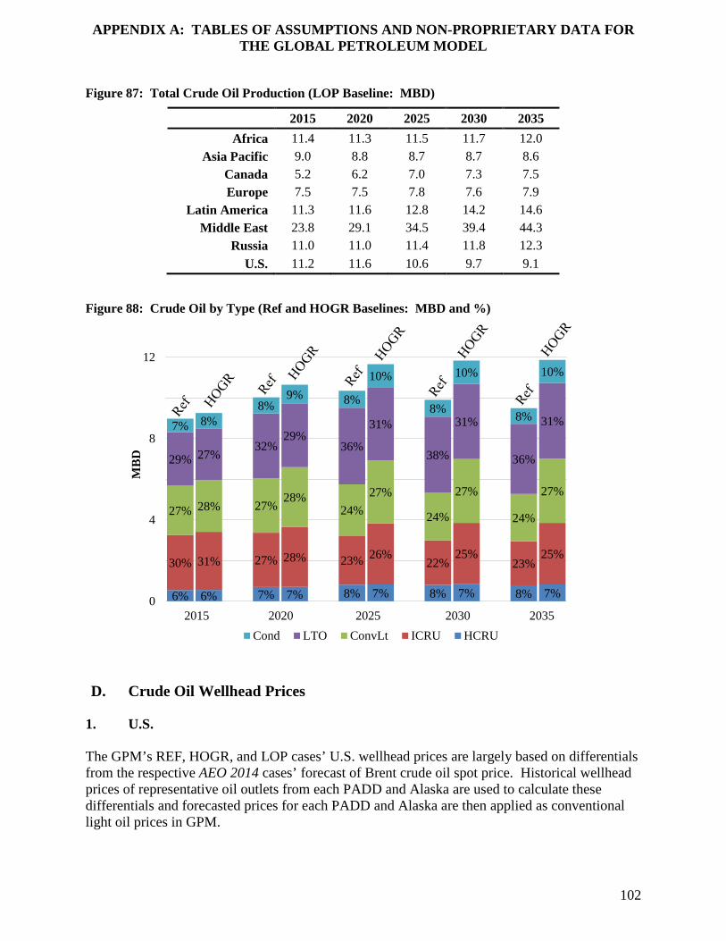
APPENDIX A: TABLES OF ASSUMPTIONS AND NON-PROPRIETARY DATA FOR THE GLOBAL PETROLEUM MODEL
102
Figure 87: Total Crude Oil Production (LOP Baseline: MBD)
2015 2020 2025 2030 2035 Africa 11.4 11.3 11.5 11.7 12.0
Asia Pacific 9.0 8.8 8.7 8.7 8.6 Canada 5.2 6.2 7.0 7.3 7.5 Europe 7.5 7.5 7.8 7.6 7.9
Latin America 11.3 11.6 12.8 14.2 14.6 Middle East 23.8 29.1 34.5 39.4 44.3
Russia 11.0 11.0 11.4 11.8 12.3 U.S. 11.2 11.6 10.6 9.7 9.1
Figure 88: Crude Oil by Type (Ref and HOGR Baselines: MBD and %)
D. Crude Oil Wellhead Prices
1. U.S.
The GPM’s REF, HOGR, and LOP cases’ U.S. wellhead prices are largely based on differentials from the respective AEO 2014 cases’ forecast of Brent crude oil spot price. Historical wellhead prices of representative oil outlets from each PADD and Alaska are used to calculate these differentials and forecasted prices for each PADD and Alaska are then applied as conventional light oil prices in GPM.
6% 6% 7% 7% 8% 7% 8% 7% 8% 7%
30% 31% 27% 28% 23% 26%22%
25%23%
25%
27% 28% 27%28%
24%27%
24%
27%
24%
27%
29% 27%32%
29%36%
31%
38%
31%
36%
31%7% 8%8%
9% 8%
10%
8%
10%
8%
10%
0
4
8
12
MB
D
Cond LTO ConvLt ICRU HCRU2015 2020 2025 2030 2035

APPENDIX A: TABLES OF ASSUMPTIONS AND NON-PROPRIETARY DATA FOR THE GLOBAL PETROLEUM MODEL
103
2. Canada
The GPM’s Ref case East Canada conventional light oil prices are set at the reference AEO 2014 forecast for Brent spot prices. Conventional light prices for West Canada are then set at a differential to Brent prices.
GPM’s Ref case Canadian production prices are also applied to the GPM HOGR case.
For the LOP case, Canadian production prices are set using the same ratio methodology described in the Canadian crude oil production section above.
3. Outside North America
Like U.S. and Canada, oil prices for the Ref case for GPM regions outside of North America are calculated from differentials off of the Brent spot prices for the AEO 2014 Reference case. These differentials are calculated using historical wellhead prices of representative oil outlets for each region and for conventional light oil, intermediate oil, and heavy oil using data sourced from various crude reports. Forecasted prices for LTO and condensates follow the same methodology as presented in the U.S. wellhead prices section above.
Ref case GPM prices are also applied to the HOGR GPM case.
For the LOP case, production prices are set using the same ratio methodology described in the Canadian crude oil production section above.
Figure 89 through Figure 95 report crude oil prices for each of the model’s regions with Canada reflecting the weighted average price of the model’s two Canadian regions and U.S. reflecting the weighted average price of the model’s U.S. sub-regions. Figure 89: Heavy Crude Oil Wellhead Prices (Ref Baseline: 2013$/bbl)
2015 2020 2025 2030 2035 Africa N/A N/A N/A N/A N/A
Asia Pacific N/A N/A N/A N/A N/A Canada $80 $77 $88 $96 $107 Europe N/A N/A N/A N/A N/A
Latin America $93 $92 $103 $112 $123 Middle East N/A N/A N/A N/A N/A
Russia $92 $91 $103 $113 $124 U.S. $94 $92 $103 $111 $122

APPENDIX A: TABLES OF ASSUMPTIONS AND NON-PROPRIETARY DATA FOR THE GLOBAL PETROLEUM MODEL
104
Figure 90: Intermediate Crude Oil Wellhead Prices (Ref Baseline: 2013$/bbl)
2015 2020 2025 2030 2035 Africa $93 $92 $103 $114 $125
Asia Pacific $95 $94 $106 $116 $127 Canada $85 $84 $96 $105 $116 Europe $94 $93 $105 $115 $127
Latin America $95 $93 $104 $114 $125 Middle East $93 $91 $103 $114 $125
Russia $94 $93 $105 $115 $127 U.S. $94 $92 $104 $113 $125
Figure 91: Conventional Light Oil Wellhead Prices (Ref Baseline: 2013$/bbl)
2015 2020 2025 2030 2035 Africa $94 $93 $104 $115 $126
Asia Pacific $96 $95 $107 $117 $129 Canada $87 $90 $97 $109 $122 Europe $95 $94 $106 $116 $128
Latin America $96 $93 $104 $115 $126 Middle East $94 $92 $104 $115 $126
Russia $95 $94 $106 $116 $128 U.S. $91 $90 $102 $113 $125
Figure 92: Light Tight Oil Wellhead Prices (Ref Baseline: 2013$/bbl)
2015 2020 2025 2030 2035 Africa $94 $93 $104 $115 $126
Asia Pacific $96 $95 $107 $117 $129 Canada $85 $83 $96 $112 $125 Europe $95 $94 $106 $116 $127
Latin America $96 $93 $104 $115 $126 Middle East N/A N/A N/A N/A N/A
Russia $95 $94 $106 $116 $128 U.S. $74 $76 $94 $109 $123

APPENDIX A: TABLES OF ASSUMPTIONS AND NON-PROPRIETARY DATA FOR THE GLOBAL PETROLEUM MODEL
105
Figure 93: Condensate Wellhead Prices (Ref Baseline: 2013$/bbl)
2015 2020 2025 2030 2035 Africa $94 $93 $104 $115 $126
Asia Pacific $96 $95 $107 $117 $129 Canada $83 $82 $94 $115 $131 Europe $95 $94 $106 $116 $127
Latin America $96 $93 $104 $115 $126 Middle East $94 $92 $104 $115 $126
Russia $95 $94 $106 $116 $128 U.S. $71 $75 $93 $108 $122
Figure 94: Average Crude Oil Wellhead Prices (HOGR Baseline: 2013$/bbl)
2015 2020 2025 2030 2035 Africa $89 $87 $97 $106 $118
Asia Pacific $81 $77 $85 $92 $102 Canada $71 $73 $83 $91 $101 Europe $86 $85 $96 $104 $116
Latin America $89 $89 $99 $108 $119 Middle East $76 $73 $81 $88 $98
Russia $84 $82 $93 $102 $113 U.S. $65 $63 $70 $75 $80
Figure 95: Average Crude Oil Wellhead Prices (LOP Baseline: 2013$/bbl)
2015 2020 2025 2030 2035 Africa $68 $61 $63 $64 $64
Asia Pacific $62 $53 $53 $52 $50 Canada $51 $45 $46 $45 $46 Europe $66 $60 $62 $63 $63
Latin America $68 $61 $63 $64 $65 Middle East $55 $50 $53 $54 $57
Russia $64 $56 $57 $57 $58 U.S. $54 $49 $46 $43 $41
E. Refined Petroleum Product Consumption
The GPM’s refined petroleum products consumption analysis is disaggregated into three categories of product: motor gasoline, distillate (which includes diesel, jet fuel, and kerosene), and all other refined petroleum products. The methodology for attaining input data at this granularity for each region is described below.

APPENDIX A: TABLES OF ASSUMPTIONS AND NON-PROPRIETARY DATA FOR THE GLOBAL PETROLEUM MODEL
106
1. U.S.
U.S. PADD regions’ refined petroleum product consumption for the REF, HOGR, and LOP cases is defined by regional level data from respective AEO 2014 scenarios such that:
• The AEO’s New England, Mid-Atlantic, and South Atlantic regions sum to GPM’s PADD 1 region.
• The AEO’s East North Central and West North Central regions sum to GPM’s PADD 2 region.
• The AEO’s East South Central and West South Central regions sum to GPM’s PADD 3 region.
• The AEO’s Mountain region sums to GPM’s PADD 4 region. • The AEO’s Pacific region sums to GPM’s PADD 5 region. • Constant rates of 0.02 million barrels per day of motor gasoline consumption, 0.01
million barrels per day of distillate consumption, and 0.02 million barrels per day of other refined petroleum products consumption are applied to GPM’s Alaska region.
2. Canada
East and West Canada regional refined petroleum product consumption for the REF and HOGR cases is defined by summing motor gasoline, distillate, and other refined petroleum products consumption from Canada’s Energy Future 2013 across the provinces included in each region, as defined above.
In Canada the LOP case demand for regions outside of the U.S. was interpolated from the AEO 2014 text and disaggregated between OECD and non-OECD regions. Worldwide Ref case demand from previously calculated GPM inputs was then aggregated to OECD and non-OECD regions and similar LOP to Ref case ratios were developed as described for the LOP production side in the Canadian production section above. These ratios were then applied to their respective Ref case region demand inputs to calculate consumption of refined petroleum products and their prices in the LOP case.
3. Outside North America
The rest of the world’s GPM regions’ REF and HOGR RPP consumption is based on world liquids consumption from the IEO 2013. Using the IEO to GPM regional mapping, we determined total liquids consumption by region from 2015 to 2035.
To break these total liquids consumption figures into the GPM’s three RPP categories, we relied on information from the WOO 2013 figure 5.2, which provides refined petroleum product demand by type and region for years 2012, 2020, and 2035.
Interpolating for the missing years from 2012 to 2035, we built a full range of WOO-based RPP consumption by type for the years 2015 to 2035.
The proportion of each RPP’s product consumption of total RPP consumption by region was then applied to its respective GPM region to break out total RPPs to motor gasoline, distillate,

APPENDIX A: TABLES OF ASSUMPTIONS AND NON-PROPRIETARY DATA FOR THE GLOBAL PETROLEUM MODEL
107
and other refined petroleum products. Regions in the WOO table were mapped to GPM regions such that:
• The WOO region Latin America mapped to GPM’s Latin America region. • The WOO region Africa mapped to GPM’s Africa region. • The WOO region Europe mapped to GPM’s Europe region. • The WOO region Russia & Caspian mapped to GPM’s Russia region. • The WOO region Middle East mapped to GPM’s Middle East region. • The WOO regions China and Other Asia-Pacific mapped to GPM’s Asia Pacific region.
For the LOP case, ratios were applied to the Ref case using the same methodology as described in the Canadian demand section above.
Figure 96 through Figure 100 report consumption of refined petroleum products for each of the model’s regions with the Canadian regions aggregated into Canada and the PADDs and Alaska regions aggregated into the U.S.
Figure 96: Gasoline Consumption (Ref Baseline: MBD)
2015 2020 2025 2030 2035 Africa 0.7 0.7 0.8 0.8 0.9
Asia Pacific 5.4 6.0 6.7 7.2 7.8 Canada 0.9 0.9 0.9 0.9 0.9 Europe 2.5 2.5 2.6 2.7 2.8
Latin America 2.6 2.8 2.9 3.1 3.3 Middle East 1.5 1.7 1.7 1.8 1.8
Russia 0.8 0.8 0.9 0.9 0.9 U.S. 7.9 7.4 6.6 6.0 5.8
Figure 97: Distillate Consumption (Ref Baseline: MBD)
2015 2020 2025 2030 2035 Africa 1.5 1.6 1.7 1.8 2.0
Asia Pacific 11.4 13.3 15.4 17.2 19.0 Canada 0.7 0.8 0.8 0.9 1.0 Europe 8.3 9.0 9.1 9.3 9.4
Latin America 3.1 3.4 3.6 3.9 4.2 Middle East 2.7 3.3 3.5 3.7 3.8
Russia 1.0 1.1 1.1 1.2 1.3 U.S. 5.4 5.7 5.9 6.1 6.1

APPENDIX A: TABLES OF ASSUMPTIONS AND NON-PROPRIETARY DATA FOR THE GLOBAL PETROLEUM MODEL
108
Figure 98: Other Refined Petroleum Products Consumption (Ref Baseline: MBD)
2015 2020 2025 2030 2035 Africa 1.2 1.2 1.2 1.3 1.3
Asia Pacific 13.3 13.9 14.3 14.6 15.1 Canada 1.3 1.4 1.5 1.6 1.6 Europe 4.9 4.4 4.3 4.2 4.2
Latin America 3.1 3.0 3.0 3.2 3.3 Middle East 3.8 3.8 3.8 3.8 4.0
Russia 1.5 1.5 1.5 1.5 1.6 U.S. 4.0 4.4 4.7 4.7 4.7
Figure 99: Total Refined Petroleum Product Demand (HOGR Baseline: MBD)
2015 2020 2025 2030 2035 Africa 3.4 3.5 3.8 4.0 4.2
Asia Pacific 29.5 32.8 36.2 39.2 42.5 Canada 2.9 3.1 3.3 3.4 3.5 Europe 15.3 15.7 15.9 16.3 16.6
Latin America 8.7 9.0 9.4 10.2 10.9 Middle East 7.8 8.5 8.8 9.1 9.5
Russia 3.3 3.4 3.5 3.7 3.8 U.S. 19.2 20.0 19.7 19.3 19.2
Figure 100: Total Refined Petroleum Product Demand (LOP Baseline: MBD)
2015 2020 2025 2030 2035 Africa 3.4 3.5 3.8 4.1 4.4
Asia Pacific 29.5 32.5 36.5 40.3 44.0 Canada 3.2 3.5 3.8 4.1 4.2 Europe 17.1 17.7 18.4 19.1 19.7
Latin America 8.7 8.9 9.5 10.5 11.2 Middle East 8.7 10.3 11.3 11.5 12.0
Russia 3.3 3.3 3.5 3.8 3.9 U.S. 16.5 17.2 17.2 17.0 17.0
F. Refined Petroleum Product Consumption Prices
GPM necessitates the use of both an end-user price for consumed products, as well as intermediate costs (which are composed of distribution costs and taxes), to model trade flows. Below we describe the methodology for collecting these data by region.

APPENDIX A: TABLES OF ASSUMPTIONS AND NON-PROPRIETARY DATA FOR THE GLOBAL PETROLEUM MODEL
109
1. U.S.
Demand prices for the Ref, HOGR, and LOP for motor gasoline and distillate in U.S. PADD regions were calculated using respective AEO 2014 regional Components of Selected Petroleum Prices tables. These tables present an end-user price, as well as taxes and distribution costs for an intermediate price.
Demand prices for other refined petroleum products in U.S. PADD regions were calculated using the residual fuel oil price from AEO 2014’s regional Energy Prices by Sector and Source tables. These tables present both an only an end-user price for residual fuel. A $0.10/gal was applied as an intermediate costs for all years to represent distribution costs, as residual fuel oil does not have associated taxes.
AEO regions were mapped to GPM PADD regions identically to as described in the U.S. RPP consumption section above. Where a GPM region was composed of multiple AEO regions, prices were averaged. To determine GPM distillate prices, AEO diesel, jet fuel, and residential distillate fuel oil/heating oil prices were weighted based on the proportion of diesel consumed in the PADD.
Refined petroleum product prices for Alaska were assumed to be equal to PADD 5 prices.
2. Canada
GPM Canadian end-user prices for the Ref and HOGR cases were calculated using data from Canada’s Energy Future 2013 Reference case Drivers and Prices tables. Motor gasoline prices across respective provinces were averaged based on consumption volumes by province to develop GPM regional motor gasoline prices. Light fuel oil and diesel prices were averaged across sectors, respective provinces, and weighted based on fuel type consumption to determine distillate prices.
GPM Canadian other refined petroleum products end-user prices were calculated by applying the national AEO 2014 U.S. price differential between motor gasoline and other refined petroleum products (other refined petroleum products category is composed of residual fuel prices, as stated above), to regional Canadian motor gasoline prices.
For motor gasoline and distillate intermediate prices, the difference between regional Canadian end-user prices and their respective national U.S. wholesale prices was applied. For other refined petroleum products intermediate prices, a constant price of $0.10/gal was applied, similar to the analogous U.S. intermediate prices.
For the LOP case, ratios were applied to Ref case prices in the same manner as described above in the Canadian demand sections.
3. Outside North America
Year 2010 motor gasoline and diesel prices are available on a country basis from publicly available data sources. Representative countries from each GPM region were chosen as a basis for the end-user prices and a price differential was determined between the country and the U.S. This differential was then applied to national AEO 2014 U.S. motor gasoline and distillate prices to calculate regional GPM Ref and HOGR end-user prices.
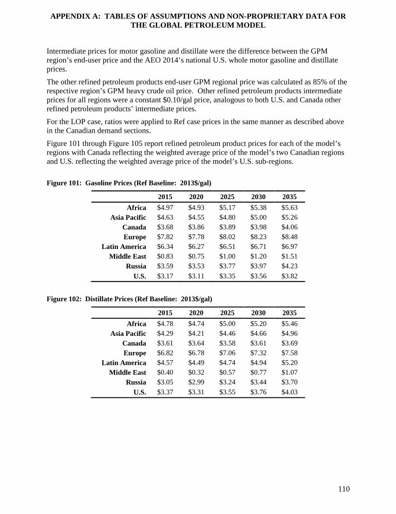
APPENDIX A: TABLES OF ASSUMPTIONS AND NON-PROPRIETARY DATA FOR THE GLOBAL PETROLEUM MODEL
110
Intermediate prices for motor gasoline and distillate were the difference between the GPM region’s end-user price and the AEO 2014’s national U.S. whole motor gasoline and distillate prices.
The other refined petroleum products end-user GPM regional price was calculated as 85% of the respective region’s GPM heavy crude oil price. Other refined petroleum products intermediate prices for all regions were a constant $0.10/gal price, analogous to both U.S. and Canada other refined petroleum products’ intermediate prices.
For the LOP case, ratios were applied to Ref case prices in the same manner as described above in the Canadian demand sections.
Figure 101 through Figure 105 report refined petroleum product prices for each of the model’s regions with Canada reflecting the weighted average price of the model’s two Canadian regions and U.S. reflecting the weighted average price of the model’s U.S. sub-regions. Figure 101: Gasoline Prices (Ref Baseline: 2013$/gal)
2015 2020 2025 2030 2035 Africa $4.97 $4.93 $5.17 $5.38 $5.63
Asia Pacific $4.63 $4.55 $4.80 $5.00 $5.26 Canada $3.68 $3.86 $3.89 $3.98 $4.06 Europe $7.82 $7.78 $8.02 $8.23 $8.48
Latin America $6.34 $6.27 $6.51 $6.71 $6.97 Middle East $0.83 $0.75 $1.00 $1.20 $1.51
Russia $3.59 $3.53 $3.77 $3.97 $4.23 U.S. $3.17 $3.11 $3.35 $3.56 $3.82
Figure 102: Distillate Prices (Ref Baseline: 2013$/gal)
2015 2020 2025 2030 2035 Africa $4.78 $4.74 $5.00 $5.20 $5.46
Asia Pacific $4.29 $4.21 $4.46 $4.66 $4.96 Canada $3.61 $3.64 $3.58 $3.61 $3.69 Europe $6.82 $6.78 $7.06 $7.32 $7.58
Latin America $4.57 $4.49 $4.74 $4.94 $5.20 Middle East $0.40 $0.32 $0.57 $0.77 $1.07
Russia $3.05 $2.99 $3.24 $3.44 $3.70 U.S. $3.37 $3.31 $3.55 $3.76 $4.03

APPENDIX A: TABLES OF ASSUMPTIONS AND NON-PROPRIETARY DATA FOR THE GLOBAL PETROLEUM MODEL
111
Figure 103 Other Refined Petroleum Products Prices (Ref Baseline: 2013$/gal)
2015 2020 2025 2030 2035 Africa $2.58 $2.52 $2.73 $2.91 $3.14
Asia Pacific $2.72 $2.66 $2.87 $3.04 $3.23 Canada $2.86 $3.11 $3.07 $3.11 $3.13 Europe $2.51 $2.48 $2.72 $2.89 $3.10
Latin America $2.53 $2.47 $2.68 $2.86 $3.09 Middle East $2.60 $2.54 $2.75 $2.92 $3.11
Russia $2.59 $2.53 $2.74 $2.91 $3.10 U.S. $2.43 $2.43 $2.63 $2.81 $3.02
Figure 104: Average Refined Petroleum Product Price (HOGR Baseline: 2013$/gal)
2015 2020 2025 2030 2035 Africa $4.07 $4.04 $4.34 $4.56 $4.83
Asia Pacific $3.69 $3.67 $3.95 $4.17 $4.45 Canada $3.18 $3.20 $3.31 $3.39 $3.49 Europe $5.68 $5.81 $6.14 $6.39 $6.69
Latin America $4.45 $4.46 $4.72 $4.93 $5.18 Middle East $1.56 $1.42 $1.63 $1.83 $2.07
Russia $3.04 $3.00 $3.25 $3.43 $3.67 U.S. $3.33 $3.26 $3.51 $3.72 $3.98
Figure 105: Average Refined Petroleum Product Price (LOP Baseline: 2013$/gal)
2015 2020 2025 2030 2035 Africa $3.61 $3.54 $3.53 $3.54 $3.60
Asia Pacific $3.24 $3.16 $3.17 $3.18 $3.25 Canada $2.74 $2.72 $2.55 $2.48 $2.42 Europe $5.23 $5.34 $5.36 $5.39 $5.43
Latin America $3.99 $3.94 $3.94 $3.94 $3.99 Middle East $1.00 $0.79 $0.74 $0.76 $0.79
Russia $2.60 $2.49 $2.47 $2.44 $2.49 U.S. $2.77 $2.65 $2.63 $2.64 $2.69
G. Refinery Inputs
The GPM sets crude oil refining capacity constraints on each region by three types of refineries: hydroskimmers, crackers, and cokers. These limitations are based on data from the December 2013 Oil and Gas Journal Worldwide Refining Report. The model refinery capacity outlook is

APPENDIX A: TABLES OF ASSUMPTIONS AND NON-PROPRIETARY DATA FOR THE GLOBAL PETROLEUM MODEL
112
based on an index derived from the growth of the model’s total refined petroleum product demand in each scenario, over time.
Figure 106: Regional Hydroskimmer Refining Capacity (MBD)
2015 2020 2025 2030 2035 PADD 1 0.1 0.1 0.1 0.1 0.1 PADD 2 0.0 0.0 0.0 0.0 0.0 PADD 3 0.4 0.4 0.4 0.4 0.4 PADD 4 0.0 0.0 0.0 0.0 0.0 PADD 5 0.3 0.3 0.3 0.3 0.3
Alaska 0.0 0.0 0.0 0.0 0.0 West Canada 0.1 0.1 0.1 0.1 0.1 East Canada 0.0 0.0 0.0 0.0 0.0
Africa 1.9 2.0 2.0 2.1 2.3 Asia Pacific 9.1 10.1 11.0 11.9 12.8
Europe 5.6 5.7 5.8 5.8 5.9 Latin America 0.7 0.8 0.8 0.8 0.9
Middle East 2.0 2.5 2.6 2.7 2.7 Russia 0.3 0.3 0.3 0.3 0.3
Figure 107: Regional Cracker Refining Capacity (MBD)
2015 2020 2025 2030 2035 PADD 1 0.8 0.8 0.8 0.8 0.9 PADD 2 1.1 1.1 1.1 1.1 1.1 PADD 3 1.4 1.5 1.6 1.6 1.6 PADD 4 0.3 0.3 0.3 0.3 0.3 PADD 5 0.4 0.4 0.4 0.4 0.4
Alaska 0.1 0.1 0.1 0.1 0.1 West Canada 1.1 1.2 1.3 1.4 1.5 East Canada 0.5 0.5 0.5 0.5 0.5
Africa 0.9 0.9 0.9 1.0 1.0 Asia Pacific 12.1 13.4 14.6 15.8 17.1
Europe 11.9 11.9 12.1 12.3 12.5 Latin America 3.6 3.9 4.1 4.2 4.5
Middle East 5.7 7.0 7.2 7.4 7.6 Russia 1.3 1.5 1.5 1.5 1.5

APPENDIX A: TABLES OF ASSUMPTIONS AND NON-PROPRIETARY DATA FOR THE GLOBAL PETROLEUM MODEL
113
Figure 108: Regional Coker Refining Capacity (MBD)
2015 2020 2025 2030 2035 PADD 1 0.3 0.3 0.4 0.4 0.4 PADD 2 2.7 2.7 2.7 2.7 2.8 PADD 3 7.5 8.0 8.1 8.1 8.1 PADD 4 0.4 0.4 0.4 0.4 0.4 PADD 5 1.9 2.0 2.0 2.0 2.0
Alaska 0.1 0.1 0.1 0.1 0.1 West Canada 0.1 0.1 0.1 0.2 0.2 East Canada 0.2 0.2 0.2 0.2 0.2
Africa 0.3 0.3 0.4 0.4 0.4 Asia Pacific 5.4 6.0 6.6 7.1 7.7
Europe 5.2 5.3 5.3 5.4 5.5 Latin America 3.5 3.8 4.0 4.1 4.3
Middle East 0.4 0.5 0.5 0.5 0.6 Russia 0.0 0.0 0.0 0.0 0.0
The model assumes that hydroskimmers can only process those GPM crude oil categories above an API gravity of 22; crackers and cokers can process all types of crude oil.
A maximum refinery utilization for each region was set using data from BP’s Statistical Review of World Energy 2013. Historical regional oil refinery throughputs were divided by oil refinery capacities to calculate regional refinery utilizations. A 5-year maximum utilization from 2008 to 2012 was then used as a basis for inputs to our model.
Figure 109: Maximum Refinery Utilization by Region (%)
Africa 74% Asia Pacific 85%
Canada 90% Europe 84%
Latin America 78% Middle East 80%
Russia 81% USA 88%

APPENDIX A: TABLES OF ASSUMPTIONS AND NON-PROPRIETARY DATA FOR THE GLOBAL PETROLEUM MODEL
114
Figure 110: Refining Costs for Hydroskimmers by Region and Type of Crude Oil (2013$/bbl)
HCRU ICRU ConvLt LTO Cond PADD 1 6.1 5.1 4.1 4.1 4.1 PADD 2 5.1 4.1 3.1 3.1 3.1 PADD 3 4.1 3.1 2.0 2.0 2.0 PADD 4 5.1 4.1 3.1 3.1 3.1 PADD 5 7.2 6.1 5.1 5.1 5.1
Alaska N/A N/A N/A N/A N/A West Canada 3.1 2.0 1.0 1.0 1.0 East Canada N/A N/A N/A N/A N/A
Africa 8.7 7.7 6.6 6.6 6.6 Asia Pacific 8.7 7.7 6.6 6.6 6.6
Europe 8.7 7.7 6.6 6.6 6.6 Latin America 8.7 7.7 6.6 6.6 6.6
Middle East 8.2 7.2 6.1 6.1 6.1 Russia 8.7 7.7 6.6 6.6 6.6
Figure 111: Refining Costs for Crackers by Region and Type of Crude Oil (2013$/bbl)
HCRU ICRU ConvLt LTO Cond PADD 1 8.2 6.1 5.1 5.1 5.1 PADD 2 7.2 5.1 4.1 4.1 4.1 PADD 3 6.1 4.1 3.1 3.1 3.1 PADD 4 7.2 5.1 4.1 4.1 4.1 PADD 5 9.2 7.2 6.1 6.1 6.1
Alaska 9.7 7.7 6.6 6.6 6.6 West Canada 5.1 3.1 2.0 2.0 2.0 East Canada 5.1 3.1 2.0 2.0 2.0
Africa 10.7 8.7 7.7 7.7 7.7 Asia Pacific 10.7 8.7 7.7 7.7 7.7
Europe 10.7 8.7 7.7 7.7 7.7 Latin America 10.7 8.7 7.7 7.7 7.7
Middle East 10.2 8.2 7.2 7.2 7.2 Russia 10.7 8.7 7.7 7.7 7.7
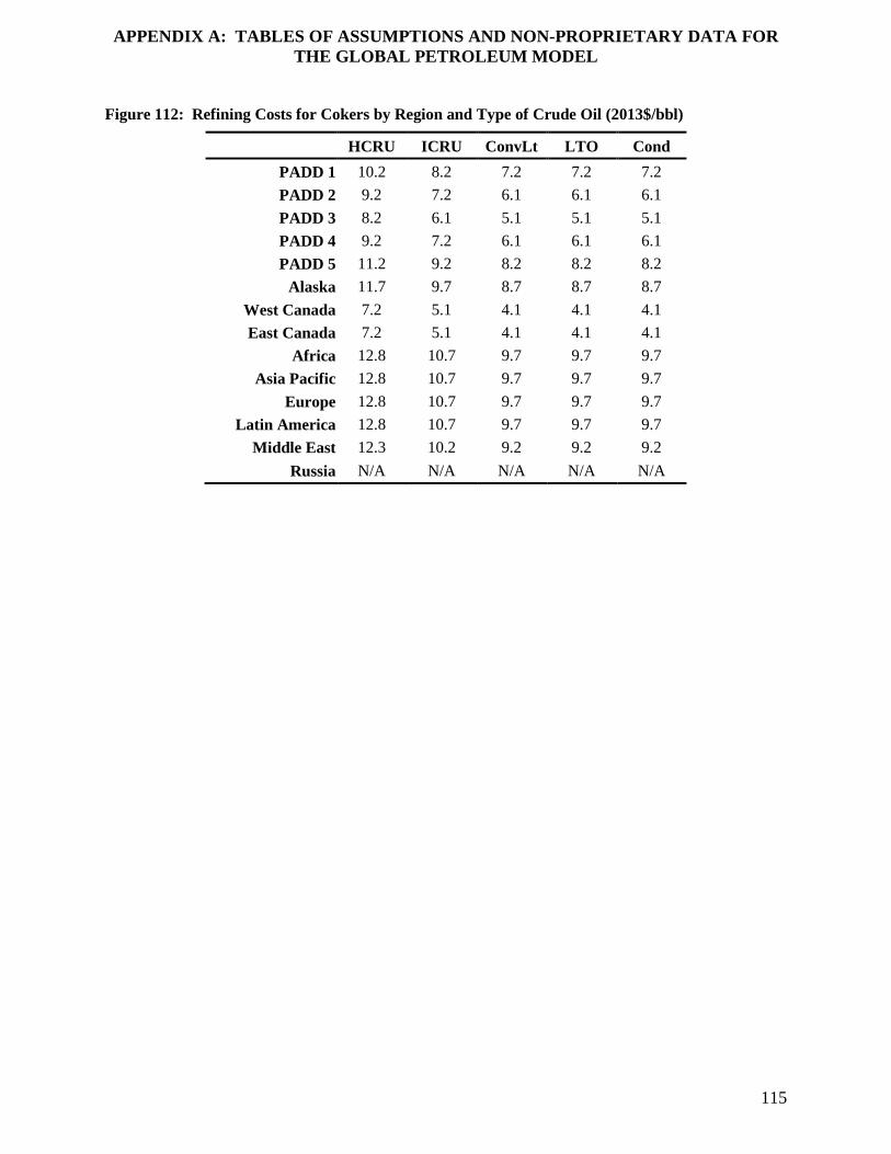
APPENDIX A: TABLES OF ASSUMPTIONS AND NON-PROPRIETARY DATA FOR THE GLOBAL PETROLEUM MODEL
115
Figure 112: Refining Costs for Cokers by Region and Type of Crude Oil (2013$/bbl)
HCRU ICRU ConvLt LTO Cond PADD 1 10.2 8.2 7.2 7.2 7.2 PADD 2 9.2 7.2 6.1 6.1 6.1 PADD 3 8.2 6.1 5.1 5.1 5.1 PADD 4 9.2 7.2 6.1 6.1 6.1 PADD 5 11.2 9.2 8.2 8.2 8.2
Alaska 11.7 9.7 8.7 8.7 8.7 West Canada 7.2 5.1 4.1 4.1 4.1 East Canada 7.2 5.1 4.1 4.1 4.1
Africa 12.8 10.7 9.7 9.7 9.7 Asia Pacific 12.8 10.7 9.7 9.7 9.7
Europe 12.8 10.7 9.7 9.7 9.7 Latin America 12.8 10.7 9.7 9.7 9.7
Middle East 12.3 10.2 9.2 9.2 9.2 Russia N/A N/A N/A N/A N/A

APPENDIX A: TABLES OF ASSUMPTIONS AND NON-PROPRIETARY DATA FOR THE GLOBAL PETROLEUM MODEL
116
H. Costs to Move Products
1. Pipeline
Transportation costs were developed to move crude oil and refined petroleum products between regions using a variety of publicly available data sources. The results are shown in the tables below.
Figure 113: Cost to Move Crude Oil through Intra- or Inter-Regional Pipelines (2013$/bbl)
From | To PADD 1
PADD 2
PADD 3
PADD 4
PADD 5 Alaska West
Canada East
Canada Africa Asia Pacific Europe Latin
America Middle
East Russia
PADD 1 $0.1 $2.0 PADD 2 $0.1 $13.3 $10.2 $4.1 $3.1 PADD 3 $8.2 $0.1 $8.2 PADD 4 $10.2 $8.2 $0.1 $3.1 PADD 5 $0.1
Alaska $0.1 West Canada $18.4 $4.1 $16.3 $3.1 $0.1 $13.3 East Canada $4.1 $13.3 $0.1
Africa $5.1 Asia Pacific $5.1
Europe $5.1 Latin America $5.1
Middle East $5.1 $10.2 $5.1 $5.1
Russia $8.2 $5.1 $5.1

APPENDIX A: TABLES OF ASSUMPTIONS AND NON-PROPRIETARY DATA FOR THE GLOBAL PETROLEUM MODEL
117
Figure 114: Cost to Move Refined Petroleum Products through Intra- or Inter-Regional Pipelines (2013$/bbl)
From | To PADD 1
PADD 2
PADD 3
PADD 4
PADD 5 Alaska West
Canada East
Canada Africa Asia Pacific Europe Latin
America Middle
East Russia
PADD 1 $0.1 $2.8 PADD 2 $0.1 $1.5 $2.0 PADD 3 $1.9 $2.5 $0.1 $1.9 $1.9 PADD 4 $0.1 $0.7 PADD 5 $0.1
Alaska $0.1 West Canada $3.3 $0.1 East Canada $0.1
Africa $5.1 Asia Pacific $5.1
Europe $5.1 Latin America $5.1
Middle East $5.1 Russia $5.1

APPENDIX A: TABLES OF ASSUMPTIONS AND NON-PROPRIETARY DATA FOR THE GLOBAL PETROLEUM MODEL
118
2. Rail
We included transportation by rail as an option for moving crude oil and refined petroleum products within North America. The inter-regional costs were based on a variety of publicly available data. Results are provided below.
Figure 115: Cost to Move Crude Oil and Refined Petroleum Products through Rail (2013$/bbl)
From | To PADD 1
PADD 2
PADD 3
PADD 4
PADD 5
West Canada
East Canada
PADD 1 $1.0 PADD 2 $15.3 $1.0 $14.3 $10.2 $15.3
$11.2
PADD 3
$14.3 $1.0 $14.3 $14.3 PADD 4
$10.2 $14.3 $1.0 $10.2 $4.6
PADD 5
$1.0 West Canada $17.4 $5.6 $18.4 $4.6 $14.3 $1.0 $11.2
East Canada $6.6 $11.2 $1.0
3. Barge
Crude oil transportation costs were determined using shipping distances from www.searates.com. These shipping distances were translated to roundtrip delivery time, including the time to load and unload the product, and an average daily rate of $61,000, based on shipping rate information in the WEO 2013, was applied to ship crude oil for all regions except between U.S. PADD regions. Because of the Jones Act, an average daily rate of $122,000 was applied for transport between U.S. PADD regions.
To calculate refined petroleum product shipping costs, the same methodology was used, except all average shipping costs were doubled.

APPENDIX A: TABLES OF ASSUMPTIONS AND NON-PROPRIETARY DATA FOR THE GLOBAL PETROLEUM MODEL
119
Figure 116: Cost to Move Crude Oil through Barge (2013$/bbl)
From | To PADD 1
PADD 3
PADD 5 Alaska East
Canada Africa Asia Pacific Europe Latin
America Middle
East Russia
PADD 1
$1.8 $4.2
$0.5 $2.0 $4.0 $1.6 $1.0 $3.1 $1.8 PADD 3 $1.8
$3.9
$1.1 $2.4 $3.9 $2.1 $1.1 $3.6 $3.4
PADD 5 $4.2 $3.9
$1.9 $2.3 $3.2 $2.2 $3.2 $1.9 $4.1 $3.5 Alaska
$1.9
$3.2 $2.2 $3.2 $1.9 $4.1 $3.5
East Canada $0.5 $1.1 $2.3
$1.9 $4.2 $1.4 $1.1 $2.9 $1.7 Africa $2.0 $2.4 $3.2
$1.9 $0.1 $3.8 $1.7 $1.9 $2.8 $4.2
Asia Pacific $4.0 $3.9 $2.2
$4.2 $3.8 $0.1 $3.3 $3.5 $2.4 $0.9 Europe $1.6 $2.1 $3.2
$1.4 $1.7 $3.3 $0.1 $1.7 $1.8 $3.7
Latin America $1.0 $1.1 $1.9
$1.1 $1.9 $3.5 $1.7 $0.1 $3.3 $3.1 Middle East $3.1 $3.6 $4.1
$2.9 $2.8 $2.4 $1.8 $3.3 $0.1 $2.8
Russia $1.8 $3.4 $3.5 $1.7 $4.2 $0.9 $3.7 $3.1 $2.8 $0.1
Figure 117: Cost to Move Refined Petroleum Products through Barge (2013$/bbl)
From | To PADD 1
PADD 3
PADD 5 Alaska East
Canada Africa Asia Pacific Europe Latin
America Middle
East Russia
PADD 1
$3.5 $8.4
$1.2 $4.6 $8.9 $3.6 $2.3 $7.0 $4.0 PADD 3 $3.5
$7.8
$2.5 $5.3 $8.6 $4.7 $2.4 $8.1 $7.6
PADD 5 $8.4 $7.8
$4.2 $5.1 $7.2 $5.0 $7.1 $4.2 $9.1 $7.9 Alaska
$4.2
$5.0
$4.2
East Canada $1.2 $2.5 $5.1
$4.3 $9.3 $3.2 $2.3 $6.5 $3.7 Africa $4.6 $5.3 $7.2
$4.3 $0.1 $8.5 $3.8 $4.2 $6.3 $9.4
Asia Pacific $8.9 $8.6 $5.0
$9.3 $8.5 $0.1 $7.4 $7.9 $5.4 $2.1 Europe $3.6 $4.7 $7.1
$3.2 $3.8 $7.4 $0.1 $3.9 $4.1 $8.3
Latin America $2.3 $2.4 $4.2 $4.2 $2.3 $4.2 $7.9 $3.9 $0.1 $7.5 $6.8 Middle East $7.0 $8.1 $9.1
$6.5 $6.3 $5.4 $4.1 $7.5 $0.1 $6.3
Russia $4.0 $7.6 $7.9 $3.7 $9.4 $2.1 $8.3 $6.8 $6.3 $0.1

APPENDIX A: TABLES OF ASSUMPTIONS AND NON-PROPRIETARY DATA FOR THE GLOBAL PETROLEUM MODEL
120
I. Elasticity
The supply elasticity remains constant across regions for most crude oil types. Depending on the ease of accessing oil resources, the U.S. market has varying elasticities than the rest of the world for certain crude oil types.
Figure 118: Regional Supply Elasticity
2015 2020 2025 2030 2035 Heavy Crude World 0.34 0.56 0.78 1.00 1.00
Intermediate Crude World 0.34 0.56 0.78 1.00 1.00 Conventional Light World 0.34 0.56 0.78 1.00 1.00
LTO U.S46. 0.90 0.99 1.08 1.17 1.17
Rest of World 0.34 0.56 0.78 1.00 1.00
Condensates U.S. 0.90 0.99 1.08 1.17 1.17
Rest of World 0.34 0.56 0.78 1.00 1.00
The demand elasticity remains constant across regions for most crude oil types.
Figure 119: Regional Demand Elasticity
2015 2020 2025 2030 2035 All RPPs World -0.13 -0.25 -0.38 -0.50 -0.50
46 The elasticity for U.S. LTO and Condensates is applied differently as described in Chapter 2 as the supply curves
in the U.S. for these fuels is piecewise linear rather than CES.

APPENDIX B: DESCRIPTION OF MODELS
121
APPENDIX B: DESCRIPTION OF MODELS
A. Global Petroleum Model
The Global Petroleum Model (GPM) is a partial-equilibrium model designed to estimate the amount of crude oil production, refined petroleum products consumption, and trade by major petroleum consuming and/or crude oil producing regions. The model maximizes the sum of consumers’ and producers’ surplus, less transportation costs, subject to mass balancing constraints and refinery, barge, rail, and pipeline capacity constraints.
1. Model Calibration
The model is modeled after the EIA’s IEO 2013 and AEO 2014, and the NEB’s Canada’s Energy Future 2013 for crude oil production, refined petroleum products consumption, wellhead price, and delivered price forecasts. Information from the IEA’s WEO 2013 and OPEC’s WOO 2013 served as a secondary source of constraints, which, combined with the EIA and NEB data, calibrated the model such that global supply equaled global demand.
For a detailed explanation of how the GPM’s data were gathered, please see Appendix A.
2. Model Formulation
The GPM is a partial-equilibrium model designed to estimate the amount of crude oil production, refined petroleum product consumption, refining, and trade by major crude oil producing and refined petroleum product consuming regions. The model is global but has particular focus on the North American market so as to better assess the impact of the U.S.’s existing crude oil export ban. The model maximizes the sum of consumers’ and producers’ surplus less transportation and refining costs, subject to mass balancing constraints and refining and transportation capacity constraints. The model is fully dynamic in that it solves simultaneously for equilibrium prices and quantities over the entire model horizon.
The model divides the world into the following 14 regions: the five U.S. PADDs, Alaska, Western and Eastern Canada, Africa, Asia Pacific, Europe, Latin America, Middle East, and Russia. These regions are largely adapted from the EIA’s IEO regional definitions, with some modifications to address the crude oil and/or refined oil-intensive regions. The model’s international RPP consumption and crude oil production projections for these regions are based upon the EIA’s AEO 2014 and IEO 2013 cases.
The model tracks crude oil from its production to its refining into RPPs and the ultimate consumption of RPPs. The model includes five types of crude oil and NGLs. Figure 16 displays the categories and their API gravity designation. The five crude oils and NGLs are transformed into the following three RPPs: gasoline, distillates, and other refined petroleum products. The model includes three types of refineries (cokers, crackers, and skimmers) that transform the five

APPENDIX B: DESCRIPTION OF MODELS
122
crude oils into the three RPPs. NGLs are assumed to go directly into the other category for RPPs.
a. Fuel supply curves
The supply of NGLs and all types of crude oil except U.S. condensate and light tight crude oil is represented by a constant elasticity of substitution (CES) supply curve (see Equation 1). Therefore, the supply curves for each of the above mentioned fuels assume that for a given percentage change in the fuel’s price, the percentage change in its production will be the same regardless of the starting price and supply. The supply curve’s elasticity dictates how the production of fuel changes when the price of the fuel changes. The elasticity of supply is assumed to increase over time reflecting the fact that production can be more responsive in the long-run than the short-run. The elasticity of supply is assumed to be invariant across regions and fuels. The elasticity starts at 0.3 and linearly increases to 1.0 by the end of the study horizon.
Equation 1: CES Supply Curve
Q(cru,t) / Q0(cru,t) = (P(cru,t) / P0(cru,t))elasticity of supply(cru)
Each supply curve is calibrated to the benchmark data points (Q0(cru.t), P0(cru.t)) for each year t, where the benchmark data points represent those described in the data section above. Q0(cru.t) represents NERA’s adjusted forecasted quantity of crude oil production by type of crude oil for year t, and P0(cru.t) represents the NERA’s adjusted forecasted wellhead price of the type of crude oil for year t.
The supply curves for U.S. condensate and LTO are piecewise linear functions. The first line segment for condensate or LTO starts at the point of no supply (or zero quantity) and the choke price. The choke price represents the price below which no fuel will be produced. For U.S. condensates, the choke point is set at $40/bbl, and the choke price for LTO is $55/bbl. The supply curves then include the reference price and quantity which match the EIA’s AEO 2014 Reference or High Oil and Gas Resources case values depending on the case modeled. For the curve that extends to the right of the EIA’s data point the piecewise linear function approximates a CES function with an elasticity that starts at 1 in 2015 and rises to 1.2 by the end of the horizon.
b. Fuel demand curves
Each model region demands each of the types of refined petroleum products: gasoline, middle distillate, and other refined petroleum products. Each region’s demand is specified by its constant elasticity of substitution (CES) demand curve (see Equation 2). The benchmark demand and price for each product is based on the EIA’s forecasts (IEO 2013 and AEO 2014) demand for refined petroleum products. The demand curve elasticity varies over time becoming

APPENDIX B: DESCRIPTION OF MODELS
123
more elastic in the long-run. The elasticity of demand however is assumed to be the same in each region and for each refined petroleum product.
Equation 2: CES Demand Curve
Q(rpp,t) / Q0(rpp,t) = (P(rpp,t) / P0(rpp,t))elasticity of demand
Each demand curve is calibrated to the benchmark data points (Q0(rpp.t), P0(rpp.t)) for each year t, where the benchmark data points represent those of the EIA’s adjusted forecasts. Q0(rpp.t) represents the EIA’s adjusted forecasted demand for natural gas for year t and P0(rpp.t) represents NERA’s forecasted end-user price for each refined petroleum product for year t. The elasticity of demand for all refined petroleum products starts at -0.1 in the first year and rises linearly to -0.5 by the end of the model horizon.
c. Model Code – Key Equations
The GPM is formulated as a non-linear program. The following text describes at a high level the GPM’s non-linear objective function and linear constraints.
Maximize: Net Present Value (Consumer Surplus + Producer Surplus – Transportation Costs – Refining Costs)
Subject to:
𝑆𝑢𝑝𝑝𝑙𝑦(𝑠, 𝑐𝑟𝑢, 𝑡) = �𝑃𝑖𝑝𝑒(𝑠,𝑑, 𝑐𝑟𝑢, 𝑡) + 𝑅𝑎𝑖𝑙(𝑠,𝑑, 𝑐𝑟𝑢, 𝑡) + 𝑆ℎ𝑖𝑝(𝑠, 𝑑, 𝑐𝑟𝑢, 𝑡)𝑑
𝐷𝑒𝑚𝑎𝑛𝑑(𝑑, 𝑐𝑟𝑢, 𝑡) = �𝑃𝑖𝑝𝑒(𝑠,𝑑, 𝑐𝑟𝑢, 𝑡) + 𝑅𝑎𝑖𝑙(𝑠,𝑑, 𝑐𝑟𝑢, 𝑡) + 𝑆ℎ𝑖𝑝(𝑠,𝑑, 𝑐𝑟𝑢, 𝑡)𝑠
� 𝑅𝑒𝑓𝑖𝑛𝑒(𝑠, 𝑐𝑟𝑢, 𝑟𝑝𝑝, 𝑟𝑒𝑓, 𝑡) ≤𝑐𝑟𝑢,𝑟𝑝𝑝
𝑅𝑒𝑓𝑖𝑛𝑖𝑛𝑔𝐶𝑎𝑝𝑎𝑐𝑖𝑡𝑦(𝑠, 𝑟𝑒𝑓, 𝑡)
𝑃𝑖𝑝𝑒(𝑠,𝑑, 𝑓, 𝑡) ≤ 𝑃𝑖𝑝𝑒𝐶𝑎𝑝𝑎𝑐𝑖𝑡𝑦(𝑠,𝑑,𝑓, 𝑡)
�𝑅𝑎𝑖𝑙(𝑠,𝑑, 𝑓, 𝑡) ≤𝑑,𝑓
𝑅𝑎𝑖𝑙𝐶𝑎𝑝𝑎𝑐𝑖𝑡𝑦(𝑠,𝑚, 𝑡)
Export constraints in the baseline (i.e., ban cases)
𝑃𝑖𝑝𝑒(𝑈𝑆,𝑁𝑜𝑛 − 𝑈𝑆, 𝑓, 𝑡) = 0
𝑅𝑎𝑖𝑙(𝑈𝑆,𝑁𝑜𝑛 − 𝑈𝑆,𝑓, 𝑡) = 0
𝑆ℎ𝑖𝑝(𝑈𝑆,𝑁𝑜𝑛 − 𝑈𝑆, 𝑓, 𝑡) = 0

APPENDIX B: DESCRIPTION OF MODELS
124
Export constraints in the Scenarios where the entire ban is lifted in 2015
𝑃𝑖𝑝𝑒.𝑢𝑝(𝑈𝑆,𝑁𝑜𝑛 − 𝑈𝑆, 𝑓, 𝑡) = 𝑃𝑖𝑝𝑒𝐶𝑎𝑝(𝑈𝑆,𝑁𝑜𝑛 − 𝑈𝑆,𝑓)
Export constraints in the Scenarios where the entire ban is lifted in 2020
𝑃𝑖𝑝𝑒(𝑈𝑆,𝑁𝑜𝑛 − 𝑈𝑆, 𝑓, "2015") = 0
𝑅𝑎𝑖𝑙(𝑈𝑆,𝑁𝑜𝑛 − 𝑈𝑆,𝑓, "2015") = 0
𝑆ℎ𝑖𝑝(𝑈𝑆,𝑁𝑜𝑛 − 𝑈𝑆,𝑓, "2015") = 0
𝑃𝑖𝑝𝑒.𝑢𝑝(𝑈𝑆,𝑁𝑜𝑛 − 𝑈𝑆, 𝑓, 𝑡) = 𝑃𝑖𝑝𝑒𝐶𝑎𝑝(𝑈𝑆,𝑁𝑜𝑛 − 𝑈𝑆,𝑓) 𝑡 ≥ 2020
Export constraints in the Scenarios where the ban is lifted in 2015 on only condensate
𝑃𝑖𝑝𝑒(𝑈𝑆,𝑁𝑜𝑛 − 𝑈𝑆,𝑓, 𝑡) = 0 𝑓 ≠ 𝐶𝑜𝑛𝑑𝑒𝑛𝑠𝑎𝑡𝑒
𝑅𝑎𝑖𝑙(𝑈𝑆,𝑁𝑜𝑛 − 𝑈𝑆, 𝑓, 𝑡) = 0 𝑓 ≠ 𝐶𝑜𝑛𝑑𝑒𝑛𝑠𝑎𝑡𝑒
𝑆ℎ𝑖𝑝(𝑈𝑆,𝑁𝑜𝑛 − 𝑈𝑆,𝑓, 𝑡) = 0 𝑓 ≠ 𝐶𝑜𝑛𝑑𝑒𝑛𝑠𝑎𝑡𝑒
Consumer Surplus = ∫𝑊ℎ𝑜𝑙𝑒𝑆𝑎𝑙𝑒𝑃𝑟𝑖𝑐𝑒(𝑑, 𝑟𝑝𝑝, 𝑡) 𝑥 ( 𝐷𝑒𝑚𝑎𝑛𝑑(𝑑,𝑟𝑝𝑝,𝑡)𝐷𝑒𝑚𝑎𝑛𝑑0(𝑑,𝑟𝑝𝑝,𝑡))
( 1𝐸𝑙𝑎𝑠𝑂𝑓𝐷𝑒𝑚𝑎𝑛𝑑(𝑑,𝑡))
Producer Surplus= ∫𝑊𝑒𝑙𝑙ℎ𝑒𝑎𝑑𝑃𝑟𝑖𝑐𝑒(𝑠, 𝑐𝑟𝑢, 𝑡) 𝑥 ( 𝑆𝑢𝑝𝑝𝑙𝑦(𝑠,𝑐𝑟𝑢,𝑡)𝑆𝑢𝑝𝑝𝑙𝑦0(𝑠,𝑐𝑟𝑢,𝑡))
( 1𝐸𝑙𝑎𝑠𝑂𝑓𝑆𝑢𝑝𝑝𝑙𝑦(𝑠,𝑐𝑟𝑢,𝑡))
Transportation Costs =
� 𝑆ℎ𝑖𝑝𝐶𝑜𝑠𝑡(𝑠,𝑑,𝑓) 𝑥 𝑆ℎ𝑖𝑝(𝑠,𝑑,𝑓, 𝑡)𝑠,𝑑,𝑓,𝑡
+ � 𝑃𝑖𝑝𝑒𝐶𝑜𝑠𝑡(𝑠,𝑑, 𝑓) 𝑥 𝑃𝑖𝑝𝑒(𝑠,𝑑,𝑓, 𝑡)𝑠,𝑑,𝑓,𝑡
+ � 𝑅𝑎𝑖𝑙𝐶𝑜𝑠𝑡(𝑠,𝑑,𝑓) 𝑥 𝑅𝑎𝑖𝑙(𝑠, 𝑑,𝑓, 𝑡)𝑠,𝑑,𝑓,𝑡

APPENDIX B: DESCRIPTION OF MODELS
125
Refining Costs =
� 𝑅𝑒𝑓𝑖𝑛𝑒𝐶𝑜𝑠𝑡(𝑠, 𝑐𝑟𝑢, 𝑟𝑝𝑝, 𝑟𝑒𝑓) 𝑥 𝑅𝑒𝑓𝑖𝑛𝑒(𝑠, 𝑐𝑟𝑢, 𝑟𝑝𝑝, 𝑟𝑒𝑓, 𝑡)𝑠,𝑐𝑟𝑢,𝑟𝑝𝑝,𝑟𝑒𝑓,𝑡
where,
RefineCost(s,cru,rpp,ref) = Cost to refine crude oil into RPPs in region s and refinery type ref.
RailCost(s,d,f) = Cost to transport crude oil or refined petroleum products by rail from supply region s to demand region d.
PipeCost(s,d,f) = Cost to transport crude oil or refined petroleum products along a pipeline from supply region s to demand region d.
ShipCost(s,d,f) = Cost to ship crude oil or refined petroleum products from supply region s to demand region d.
Refine(s,cru,rpp,ref,t) = Amount of crude oil refined into refined petroleum product rpp at refinery ref in year t in region s.
Rail(s,d,f,t) = Amount of fuel f transported by rail from supply region s to demand region d in year t.
Pipe (s,d,f,t) = Amount of fuel f transported by pipeline from supply region s to demand region d in year t.
Ship(s,d,f,t) = Amount of fuel f transported by marine from supply region s to demand region d in year t.
The supply curves capture the technological issues (penetration rate, availability and cost) for the crude oil in each region. The demand curves for refined petroleum products capture the change in utility from consuming RPPs.
The constraints on U.S. exports of crude oil are applied to the baseline. Then these constraints are modified to reflect how the crude oil export ban changes in the scenario. The above model description shows the set of constraints used in the baseline (with the ban) and the scenarios (without the ban).

APPENDIX B: DESCRIPTION OF MODELS
126
B. NewERA Model
1. Overview of the NewERA Macroeconomic Model
The NewERA macro model is a forward-looking, dynamic, computable general equilibrium model of the United States. The model simulates all economic interactions in the U.S. economy, including those among industry, households, and the government. The economic interactions are based on the IMPLAN47 2008 database for a benchmark year, which includes regional detail on economic interactions among 440 different economic sectors. The macroeconomic and energy forecasts that are used to project the benchmark year going forward are calibrated to the most recent AEO 2014 produced by the Energy Information Administration (EIA). Because the model is calibrated to an internally-consistent energy forecast, the use of the model is particularly well-suited to analyze economic and energy policies and environmental regulations.
2. Model Data (IMPLAN and EIA)
The economic data is taken from the IMPLAN 2008 database, which includes balanced Social Accounting Matrices for all states in 2008. These inter-industry matrices provide a snapshot of the economy. Since the IMPLAN database contains only economic values, we benchmark energy supply, demand, trade, and prices to EIA historical statistics to capture the physical energy flows. The integration of the EIA energy quantities and prices into the IMPLAN economic database results in a balanced energy-economy dataset.
Future economic growth is calibrated to macroeconomic GDP, energy supply, energy demand, and energy price forecasts from the EIA AEO 2014. Labor productivity, labor growth, and population forecasts from the U.S. Census Bureau are used to project labor endowments along the baseline and ultimately employment by industry.
3. Brief Discussion of Model Structure
The theoretical construct behind the NewERA model is based on the circular flow of goods, services, and payments in the economy (every economic transaction has a buyer and a seller whereby goods/service go from a seller to a buyer and payment goes from the seller to the buyer). As shown in Figure 120, the model includes households, businesses, government, financial markets, and the rest of the world economy as they interact economically in the global economy. Households provide labor and capital to businesses, taxes to the government, and savings to financial markets, while also consuming goods and services and receiving government subsidies. Businesses produce goods and services, pay taxes to the government and use labor and capital. Businesses are both consumers and producers of capital for investment in the rest of
47 IMPLAN produces unique set of national structural matrices. The structural matrices form the basis for the inter-
industry flows which we use to characterize the production, household, and government transactions, see www.implan.com.
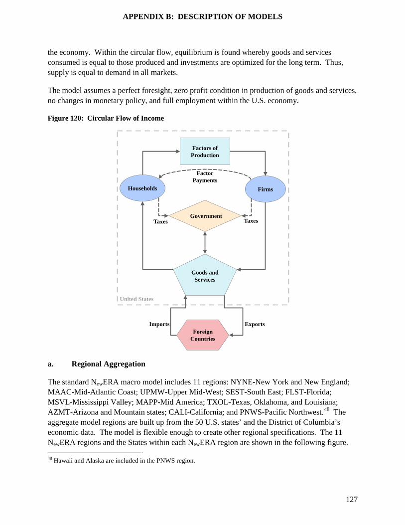
APPENDIX B: DESCRIPTION OF MODELS
127
the economy. Within the circular flow, equilibrium is found whereby goods and services consumed is equal to those produced and investments are optimized for the long term. Thus, supply is equal to demand in all markets.
The model assumes a perfect foresight, zero profit condition in production of goods and services, no changes in monetary policy, and full employment within the U.S. economy.
Figure 120: Circular Flow of Income
a. Regional Aggregation
The standard NewERA macro model includes 11 regions: NYNE-New York and New England; MAAC-Mid-Atlantic Coast; UPMW-Upper Mid-West; SEST-South East; FLST-Florida; MSVL-Mississippi Valley; MAPP-Mid America; TXOL-Texas, Oklahoma, and Louisiana; AZMT-Arizona and Mountain states; CALI-California; and PNWS-Pacific Northwest.48 The aggregate model regions are built up from the 50 U.S. states’ and the District of Columbia’s economic data. The model is flexible enough to create other regional specifications. The 11 NewERA regions and the States within each NewERA region are shown in the following figure. 48 Hawaii and Alaska are included in the PNWS region.
Households Firms
Factors of Production
Foreign Countries
Goods andServices
United States
Factor Payments
Taxes
ExportsImports
TaxesGovernment

APPENDIX B: DESCRIPTION OF MODELS
128
For this Study we aggregate the 50 states into two regions: Lower-48 region49 and Alaska state region. We disaggregate Alaska as a separate region because the crude oil ban does not apply to Alaska and only applies to the Lower-48 states.
Figure 121: Standard NewERA Model’s Macroeconomic Regions
b. Sectoral Aggregation
The NewERA model includes 12 sectors: six energy sectors (coal, natural gas, crude oil, electricity, and refined petroleum products) and seven non-energy sectors (services, manufacturing, energy-intensive, agriculture, and commercial transportation excluding trucking and motor vehicles). We represent a single type of crude oil and refined petroleum product. These sectors are aggregated up from the 440 IMPLAN sectors to 28 sectors, defined as the AEO 2014 sector in Figure 122. These 28 sectors’ economic and energy data are consistent with IMPLAN and EIA, respectively. For this study, we further aggregate these 28 production sectors into 12 production sectors. The mapping of the sectors is shown below in Figure 122. The model has the flexibility to represent sectors at any level of aggregation.
49 The Lower 48 region includes Hawaii, but since Hawaii produces no crude oil, we use the common nomenclature
Lower-48.

APPENDIX B: DESCRIPTION OF MODELS
129
Figure 122: NewERA Sectoral Representation in Core Scenarios50
c. Production and Consumption Characterization
Behavior of households, industries, investment, and government is characterized by nested CES production or utility functions. Under such a CES structure, inputs substitute against each other in a nested form. The ease of substitutability is determined by the value of the elasticity of substitution between the inputs. The greater the value of the substitution elasticity between the inputs; the greater the possibility of tradeoffs.
The CES nesting structure defines how inputs to a production activity compete with each other. In the generic production structure, intermediate inputs are aggregated in fixed proportion with a composite of energy and value-added inputs. The energy input aggregates fossil and non-fossil
50 We expand our default sectoral definition for the chemicals analysis to include ethane as an additional commodity
and three additional sectors representing chemicals subsectors. We describe these additions in detail in Chapter VIII.

APPENDIX B: DESCRIPTION OF MODELS
130
energy sources, and the value-added input combine capital and labor. Sectors with distinctive production characteristics are represented with structures different from the generic form. For alternative transportation fuels, such as ethanol and bio-diesel, inputs are demanded in fixed proportion. The characterization of nonrenewable resource supply adds a fixed resource that is calibrated to a declining resource base over time, so that it implies decreasing returns to scale. This also implies rising marginal costs of production over time for exhaustible resources. The detailed nesting structure of the households and production sectors, with assumed elasticity of substitution parameters, is shown in figures below.
i. Households
Consumers are represented by a single representative household. The representative household derives utility from both consumption of goods and services, transportation services, and leisure. The utility is represented by a nested CES utility function. The elasticity of substitution parameters between goods are shown in Figure 123.
Figure 123: NewERA Household Representation
ii. Electric Sector
We assume a simple representation of the electric sector. The electric sector models natural gas, coal, and oil-fired generation. The representation of the production is shown below.
Energy+ValueAdded
Energy ValueAdded
Capital LaborFossil Fuels Electricity
Coal Gas
σ = [ 0.35 - 0.6 ]
σ = [ 0.1 - 0.5 ]
......
σ = 1σ = [ 0.2 – 0.4 ]
σ = 0.5
Materials
σ = 0
Personal Transportation Services (VMT)
Non-Transportationσ = 0.5
Heating Oil
σ = 0.4
Leisure
σ = 0.5
Household Utility

APPENDIX B: DESCRIPTION OF MODELS
131
Figure 124: NewERA Electricity Sector Representation
iii. Other Sectors
The trucking and commercial transportation sector production structure is shown in Figure 125. The trucking sector uses diesel as transportation fuel. This sector has limited ability to substitute into other fossil fuels. The other industrial sectors (agriculture, manufacturing, energy-intensive, and motor vehicles production) and the services sector production structure, with assumed elasticity of substitution, are shown in Figure 126.
iv. Refinery Sector
In the model, each region has a single representative refinery sector that has a production structure similar to other industrial sector. We assume that the refined petroleum product is traded in the world refined petroleum markets – a homogenous good, and responds to a single world refined petroleum price. This means that the domestic price of refined petroleum product is set at the world price.
Materials
Electricity Generation
Energy+ValueAdded
Energy ValueAdded
Capital LaborFossil Fuels Electricity
Oil
σ = 0
σ = [ 0.1 - 0.5 ]
......
σ = 0
σ = 1σ = 0
σ = 0.1
Coal+Gas
Coal Gas
σ = 1.25

APPENDIX B: DESCRIPTION OF MODELS
132
Figure 125: NewERA Trucking and Commercial Transportation Sector Representation
Figure 126: NewERA Other Production Sector Representation
Materials+Oil
Commercial Transportation and Trucking Sector
Energy+ValueAdded
Energy ValueAdded
Capital LaborFossil Fuels Electricity
Coal Gas
σ = 0
σ = [ 0.1 - 0.5 ]
......
σ = 0.4
σ = 1σ = 0.4
σ = 0.5
Materials
σ = 0
Transportation Fuel
Materials
All Other Goods and Services
Energy+ValueAdded
Energy ValueAdded
Capital LaborFossil Fuels Electricity
Coal OilGas
σ = 0
σ = 0.5
......σ = 0
σ = 1σ = 0.4
σ = 0.5

APPENDIX B: DESCRIPTION OF MODELS
133
v. Exhaustible Resource Sector
The simplest characterization of non-renewable resource supply adds a fixed resource that is calibrated to decline over time, so that the decreasing returns to scale implied for the non-resource inputs lead to rising marginal costs of production over time. The top level elasticity of substitution parameter is calibrated to be consistent with resource supply elasticity. We assume the natural gas resource supply elasticity varies with the U.S. resource supply scenario. For the Ref scenario, the elasticity of supply for natural gas begins at 0.3 and increases to 0.7 by 2038. Crude oil and coal supply elasticities are invariant across the different baselines. Crude oil supply elasticity is assumed to be 0.3 in 2013 and 1.0 in 2038. Coal supply elasticity is assumed to be 0.4 in 2010 and 1.5 in 2038. The production structure of natural gas, crude oil, and coal is shown below.
Production from the crude oil, natural gas, and coal sector is either supplied to the domestic market or exported. Crude oil that is supplied to the domestic market is comingled with imported crude oil and is supplied to the domestic refinery. Natural gas and coal also follow a similar supply chain.
Figure 127: NewERA Resource Sector Representation
d. Trade Structure
All goods and services, except refined petroleum product, are treated as Armington goods, which assume that domestic and foreign goods are differentiated and thus, are imperfect substitutes. The level of imports depends upon the elasticity of substitution between the imported and domestic goods. The Armington elasticity among imported goods is assumed to be twice as large as the elasticity between domestic and aggregate imported goods, characterizing greater substitutability among imported goods.
Sector Specific
Resource
Exhaustible Resource
Non-Resource Inputs
Material Capital
σ = 0
Resource σ
Labor

APPENDIX B: DESCRIPTION OF MODELS
134
We balance the international trade account in the NewERA model by constraining changes in the current account deficit over the model horizon. The condition is that the net present value of the foreign indebtedness over the model horizon remains at the benchmark year level. This prevents distortions in economic effects that would result from perpetual increases in borrowing, but does not overly constrain the model by requiring current account balances in each year.
This treatment of the current account deficit does not mean that there cannot be trade benefits from crude oil exports. Although trade will be in balance over time, the terms of trade shift in favor of the U.S. because gains from lifting of the crude oil export ban. That is, by exporting goods of greater value, in this study it is the incremental crude oil exports, to overseas customers, the U.S. is able to import larger quantities of goods than it would be able to if the same domestic resources were devoted to producing exports of lesser value. Allowing high-value exports to proceed has a similar effect on terms of trade as would an increase in the world price of existing exports or an increase in productivity in export industries. In all these cases, the U.S. gains more imported goods in exchange for the same amount of effort being devoted to production of goods for export. The opposite is also possible, in that a fall in the world price of U.S. exports or a subsidy that promoted exports of lesser value would move the terms of trade against the U.S., in that with the same effort put into producing exports the U.S. would receive less imports in exchange and terms of trade would move against the U.S. The fact that crude oil export will only happen if there is sufficient market demand ensures that terms of trade will improve if crude oil exports occur. If the domestic price is favorable then the gains from trade would be even higher.
e. Investment Dynamics
Periods in the model are linked by capital and investment dynamics. Capital turnover in the model is represented by the standard process that capital at time t + 1 equals capital at time t plus investment at time t minus depreciation. The model optimizes consumption and savings decisions in each period, taking account of changes in the economy over the entire model horizon with perfect foresight. The consumers forego consumption to save for current and future investment.
f. Model Assumptions
The underlying assumptions of labor growth and initial capital stock drive the economy over time in the model. The model assumes full employment in the labor market. This assumption means total labor demand in a policy scenario would be the same as the baseline labor projection. The baseline labor projections are based on population growth and labor productivity forecasts over time. Hence, the labor projection can be thought to be a forecast of efficient labor units. The model assumes that labor is fungible across sectors. That is, labor can move freely out of one production sector into another without any adjustment costs or loss of productivity. Like labor, each region is endowed with its own capital stock and can move across sectors without any adjustment cost.

APPENDIX B: DESCRIPTION OF MODELS
135
Energy intensities are calibrated to the EIA projections. The differentiated energy intensities across regions result in different responses in energy supply and demand as energy price changes.
The NewERA macroeconomic model includes a simple tax representation. The model includes only two types of input taxes: marginal tax rates on capital and labor. The tax rates are based on the NBER TAXSIM model. Other indirect taxes such as excise and sales are included in the output values and not explicitly modeled.
The NewERA macro model is solved through 2035, starting from 2015 in five-year time intervals.
g. Advantages of the Macro Model Framework
The NewERA model incorporates EIA energy quantities and energy prices into the IMPLAN Social Accounting Matrices. This in-house developed approach results in a balanced energy-economy dataset that has internally consistent energy benchmark data, as well as IMPLAN consistent economic values.
The macro model incorporates all production sectors and final demanders of the economy and is linked through terms of trade. The effects of policies are transmitted throughout the economy as all sectors and agents in the economy respond until the economy reaches equilibrium. The ability of the model to track these effects and substitution possibilities across sectors and regions makes it a unique tool for analyzing policies, such as those involving energy and environmental regulations. These general equilibrium substitution effects, however, are not fully captured in a partial equilibrium framework or within an input-output modeling framework. The smooth production and consumption functions employed in this general equilibrium model enable gradual substitution of inputs in response to relative price changes, thus, avoiding all or nothing solutions.
Business investment decisions are informed by future policies and outlook. The forward-looking characteristic of the model enables businesses and consumers to determine the optimal savings and investment while anticipating future policies with perfect foresight. The alternative approach on savings and investment decisions is to assume agents in the model are myopic, thus, have no expectations for the future. Though both approaches are equally unrealistic to a certain extent, the latter approach can lead the model to produce inconsistent or incorrect impacts from an announced future policy.
The CGE modeling tool such as the NewERA macro model can analyze scenarios or policies that call for large shocks outside historical observation. Econometric models are unsuitable for policies that impose large impacts because these models’ production and consumption functions remain invariant under the policy. In addition, econometric models assume that the future path depends on the past experience and therefore fail to capture how the economy might respond under a different and new environment. For example, an econometric model cannot represent changes in fuel efficiency in response to increases in energy prices. However, the NewERA macro model can consistently capture future policy changes that envisage having large effects.

APPENDIX B: DESCRIPTION OF MODELS
136
The modeling tool is also helpful to analyze the effects of price control mechanism, such as, lifting of the crude oil export ban analyzed in this study. The model captures initial price distortion associated with imposing a ban along the baseline. By lifting the ban, and hence the price distortions, we are able to analyze efficiency gain and other benefits associated with terms of trade in a consistent manner within this framework.
The NewERA macro model is also a unique tool that can iterate over sequential policies to generate consistent equilibrium solutions starting from an internally consistent equilibrium baseline forecast (such as the AEO 2014 Reference and High Oil & Gas Resource cases). This ability of the model is particularly helpful to decompose macroeconomic effects of individual policies. For example, if one desires to perform economic analysis of a policy that includes multiple regulations, the NewERA modeling framework can be used as a tool to layer in one regulation at a time to determine the incremental effects of each policy.
h. Model Outputs
The NewERA model outputs include supply and demand of all goods and services, prices of all commodities, and terms of trade effects (including changes in imports and exports). The model outputs also include gross regional product, consumption, investment, disposable income, and changes in income from labor, capital, and resources.

APPENDIX C: TABLES AND MODEL RESULTS
137
APPENDIX C: TABLES AND MODEL RESULTS
A. Global Petroleum Model51
The following figures present detailed results from the Global Petroleum Model for each of the 18 scenarios run as part of this study. The table below provides an explanation of selected abbreviations that appear in the figures. Global Petroleum Model Acronyms and Abbreviations
LTO Light Tight Crude Oil
Cond Condensate
RPP Refined Petroleum Product
ROW Rest of World
MBD Million Barrels per Day
51 All crude oil export, import, net export and net import numbers include NGLs.

APPENDIX C: TABLES AND MODEL RESULTS
138
Figure 128: U.S. and International Reference Cases with Ban In-Effect; OPEC Competes in the Market
Results for Scenario: Ban_Ref
U.S. ROW
2015 2020 2025 2030 2035 2015 2020 2025 2030 2035
Crude Oil Production (MBD) LTO 2.6 3.2 3.8 3.7 3.5 0.8 0.9 1.6 1.7 2.0 Cond 0.7 0.8 0.8 0.8 0.8 3.3 3.6 3.9 4.4 4.8
Other Crude 8.4 9.0 9.0 8.7 8.7 73.8 77.1 79.4 83.0 87.0 Total 11.7 13.0 13.6 13.3 12.9 77.9 81.6 84.9 89.1 93.7
Crude Oil Trade (MBD)
Exports LTO 0.0 0.0 0.0 0.0 0.0 0.2 0.4 1.0 0.9 0.8 Cond 0.0 0.0 0.0 0.0 0.0 1.7 1.9 2.0 1.4 0.8
Other Crude 0.5 0.7 0.7 0.6 0.7 36.6 37.7 39.2 42.3 45.9 Total 0.5 0.7 0.8 0.6 0.8 38.5 39.9 42.1 44.6 47.4
Imports LTO 0.0 0.0 0.0 0.0 0.2 0.2 0.4 1.0 0.9 0.6 Cond 0.0 0.0 0.0 0.0 0.0 1.7 1.9 2.0 1.4 0.8
Other Crude 7.6 7.7 8.0 7.9 8.2 29.6 30.6 31.9 35.0 38.4 Total 7.6 7.7 8.0 7.9 8.4 31.5 32.9 34.9 37.3 39.8
Net Imports 7.0 7.1 7.2 7.3 7.6 -7.0 -7.1 -7.2 -7.3 -7.6
Crude Oil Price (2013$/bbl) LTO $74 $76 $94 $109 $123 $91 $89 $104 $116 $127 Cond $94 $92 $104 $113 $125 $93 $92 $104 $114 $125
Average Crude Price $86 $85 $99 $111 $124 $93 $92 $103 $113 $124
Total RPP Demand (MBD)
17.2 17.5 17.2 16.8 16.5 72.4 77.1 81.3 85.6 90.1
Total RPP Production (MBD)
18.8 20.0 20.8 20.6 20.5 70.8 74.6 77.7 81.8 86.1
RPP Trade (MBD) Exports 3.9 4.3 5.1 5.3 5.5 7.3 6.2 6.3 6.1 6.4 Imports 2.3 1.7 1.5 1.5 1.5 8.9 8.8 9.9 9.9 10.4
Net -1.6 -2.6 -3.6 -3.8 -4.0 1.6 2.6 3.6 3.8 4.0
RPP Price (2013$/gal) Gasoline $3.17 $3.11 $3.35 $3.56 $3.82 $4.97 $4.89 $5.13 $5.34 $5.60
Average RPP Price $2.55 $2.50 $2.75 $2.97 $3.24 $2.60 $2.55 $2.81 $3.03 $3.31
Refiners' Margin (2013$/bbl) $16.8 $15.8 $13.6 $12.4 $12.1 $14.3 $13.6 $12.9 $11.8 $12.1

APPENDIX C: TABLES AND MODEL RESULTS
139
Figure 129: U.S. and International Reference Cases with Crude Oil Export Ban Lifted in 2015; OPEC Competes in the Market
Results for Scenario: NoBan_Ref
U.S. ROW
2015 2020 2025 2030 2035 2015 2020 2025 2030 2035
Crude Oil Production (MBD) LTO 4.0 4.3 4.1 3.9 3.6 0.8 0.9 1.6 1.7 2.0 Cond 0.9 1.0 0.9 0.9 0.8 3.2 3.5 3.9 4.4 4.8
Other Crude 8.4 9.0 9.0 8.7 8.7 72.7 76.2 79.0 82.8 86.9 Total 13.2 14.3 14.0 13.5 13.1 76.7 80.6 84.5 88.9 93.6
Crude Oil Trade (MBD)
Exports LTO 1.4 1.5 1.0 1.1 0.5 0.3 0.4 1.1 1.1 0.8 Cond 0.6 0.4 0.3 0.1 0.2 1.6 1.8 1.9 2.3 0.5
Other Crude 0.2 0.6 0.8 1.0 1.2 35.9 37.3 39.1 41.1 46.1 Total 2.2 2.5 2.2 2.3 1.9 37.7 39.5 42.1 44.5 47.4
Imports LTO 0.1 0.1 0.2 0.3 0.4 1.6 1.8 2.0 1.9 0.9 Cond 0.0 0.0 0.1 0.2 0.1 2.1 2.2 2.1 2.2 0.6
Other Crude 7.5 8.1 8.6 8.8 8.8 28.6 29.8 31.3 33.3 38.4 Total 7.6 8.2 8.8 9.3 9.3 32.3 33.8 35.4 37.4 39.9
Net Imports 5.4 5.7 6.7 7.1 7.4 -5.4 -5.7 -6.7 -7.1 -7.4
Crude Oil Price (2013$/bbl) LTO $86 $86 $99 $112 $125 $87 $87 $103 $115 $127 Cond $91 $91 $103 $113 $125 $89 $90 $103 $114 $125
Average Crude Price $88 $88 $101 $112 $124 $89 $90 $102 $113 $124
Total RPP Demand (MBD)
17.3 17.5 17.2 16.8 16.5 72.7 77.4 81.3 85.6 90.2
Total RPP Production (MBD)
18.7 20.0 20.7 20.6 20.5 71.3 74.9 77.8 81.9 86.2
RPP Trade (MBD) Exports 3.7 4.4 4.9 5.3 5.5 7.6 6.7 6.0 5.9 6.5 Imports 2.3 1.9 1.4 1.5 1.6 9.0 9.2 9.4 9.7 10.5
Net -1.4 -2.4 -3.5 -3.7 -4.0 1.4 2.4 3.5 3.7 4.0
RPP Price (2013$/gal) Gasoline $3.07 $3.07 $3.35 $3.55 $3.82 $4.88 $4.86 $5.12 $5.33 $5.60
Average RPP Price $2.46 $2.46 $2.75 $2.96 $3.24 $2.51 $2.52 $2.81 $3.03 $3.30
Refiners' Margin (2013$/bbl) $13.1 $13.0 $12.9 $11.5 $11.4 $14.4 $14.3 $13.4 $11.9 $12.0

APPENDIX C: TABLES AND MODEL RESULTS
140
Figure 130: U.S. and International Reference Cases with Crude Oil Export Ban Lifted in 2020; OPEC Competes in the Market
Results for Scenario: NoBanDelay_Ref
U.S. ROW
2015 2020 2025 2030 2035 2015 2020 2025 2030 2035
Crude Oil Production (MBD) LTO 2.6 4.3 4.1 3.9 3.6 0.8 0.9 1.6 1.7 2.0 Cond 0.7 1.0 0.9 0.9 0.8 3.3 3.5 3.9 4.4 4.8
Other Crude 8.4 9.0 9.0 8.7 8.7 73.8 76.2 79.0 82.8 86.9 Total 11.7 14.3 14.0 13.5 13.1 77.9 80.6 84.5 88.9 93.6
Crude Oil Trade (MBD)
Exports LTO 0.0 1.5 1.0 1.1 0.5 0.2 0.4 1.1 1.1 0.8 Cond 0.0 0.4 0.3 0.1 0.2 1.7 1.8 1.9 2.3 0.5
Other Crude 0.5 0.6 0.8 1.0 1.2 36.6 37.3 39.1 41.1 46.1 Total 0.5 2.5 2.2 2.3 1.9 38.5 39.5 42.1 44.5 47.4
Imports LTO 0.0 0.1 0.2 0.3 0.4 0.2 1.8 2.0 1.9 0.9 Cond 0.0 0.0 0.1 0.2 0.1 1.7 2.2 2.1 2.2 0.6
Other Crude 7.6 8.1 8.6 8.8 8.8 29.6 29.8 31.3 33.3 38.4 Total 7.6 8.2 8.8 9.3 9.3 31.5 33.8 35.4 37.4 39.9
Net Imports 7.1 5.7 6.7 7.1 7.4 -7.1 -5.7 -6.7 -7.1 -7.4
Crude Oil Price (2013$/bbl) LTO $74 $86 $99 $112 $125 $91 $87 $103 $115 $127 Cond $94 $91 $103 $113 $125 $93 $90 $103 $114 $125
Average Crude Price $86 $88 $101 $112 $124 $93 $90 $102 $113 $124
Total RPP Demand (MBD)
17.2 17.5 17.2 16.8 16.5 72.4 77.4 81.3 85.6 90.2
Total RPP Production (MBD)
18.8 20.0 20.7 20.6 20.5 70.8 74.9 77.8 81.9 86.2
RPP Trade (MBD) Exports 3.9 4.4 4.9 5.3 5.5 7.3 6.7 6.0 5.9 6.5 Imports 2.3 1.9 1.4 1.5 1.6 8.9 9.2 9.4 9.7 10.5
Net -1.6 -2.4 -3.5 -3.7 -4.0 1.6 2.4 3.5 3.7 4.0
RPP Price (2013$/gal) Gasoline $3.17 $3.07 $3.35 $3.55 $3.82 $4.97 $4.86 $5.12 $5.33 $5.60
Average RPP Price $2.55 $2.46 $2.75 $2.96 $3.24 $2.60 $2.52 $2.81 $3.03 $3.30
Refiners' Margin (2013$/bbl) $16.8 $13.0 $12.9 $11.5 $11.4 $14.3 $14.3 $13.4 $11.9 $12.0

APPENDIX C: TABLES AND MODEL RESULTS
141
Figure 131: U.S. and International Reference Cases with Condensate Export Ban Lifted in 2015; OPEC Competes in the Market
Results for Scenario: NoBanCond_Ref
U.S. ROW
2015 2020 2025 2030 2035 2015 2020 2025 2030 2035
Crude Oil Production (MBD) LTO 3.1 3.8 4.1 3.9 3.5 0.8 0.9 1.6 1.7 2.0 Cond 0.9 0.9 0.9 0.9 0.8 3.2 3.6 3.9 4.4 4.8
Other Crude 8.4 9.0 9.0 8.7 8.7 73.3 76.6 79.1 82.9 86.9 Total 12.4 13.7 13.9 13.5 13.0 77.4 81.1 84.6 89.0 93.6
Crude Oil Trade (MBD)
Exports LTO 0.0 0.0 0.0 0.0 0.0 0.3 0.4 1.0 1.1 0.8 Cond 0.7 0.8 0.7 0.6 0.6 1.6 1.8 1.9 1.8 0.4
Other Crude 0.5 0.6 0.8 0.6 0.7 36.2 37.4 39.0 41.6 46.1 Total 1.2 1.4 1.5 1.2 1.3 38.1 39.6 41.9 44.5 47.3
Imports LTO 0.0 0.0 0.0 0.2 0.4 0.3 0.4 1.0 0.9 0.4 Cond 0.0 0.0 0.0 0.1 0.1 2.4 2.6 2.6 2.4 0.9
Other Crude 7.6 7.7 8.3 8.1 8.3 29.1 30.3 31.5 34.1 38.5 Total 7.6 7.7 8.4 8.3 8.7 31.7 33.3 35.0 37.4 39.9
Net Imports 6.4 6.4 6.9 7.1 7.5 -6.4 -6.4 -6.9 -7.1 -7.5
Crude Oil Price (2013$/bbl) LTO $77 $79 $98 $111 $124 $86 $86 $103 $115 $127 Cond $93 $91 $103 $113 $124 $91 $91 $103 $114 $125
Average Crude Price $86 $86 $101 $112 $124 $91 $90 $103 $113 $124
Total RPP Demand (MBD)
17.2 17.5 17.2 16.8 16.5 72.5 77.2 81.3 85.6 90.1
Total RPP Production (MBD)
18.8 20.0 20.8 20.6 20.5 71.0 74.7 77.7 81.9 86.2
RPP Trade (MBD) Exports 3.9 4.3 5.0 5.3 5.5 7.4 6.5 6.2 6.0 6.5 Imports 2.3 1.8 1.4 1.5 1.5 9.0 9.0 9.8 9.8 10.5
Net -1.6 -2.5 -3.6 -3.7 -4.0 1.6 2.5 3.6 3.7 4.0
RPP Price (2013$/gal) Gasoline $3.12 $3.09 $3.35 $3.56 $3.82 $4.93 $4.88 $5.12 $5.33 $5.60
Average RPP Price $2.51 $2.48 $2.75 $2.96 $3.24 $2.56 $2.54 $2.81 $3.03 $3.31
Refiners' Margin (2013$/bbl) $15.4 $15.0 $13.1 $11.8 $11.7 $14.4 $14.1 $13.3 $11.9 $12.2

APPENDIX C: TABLES AND MODEL RESULTS
142
Figure 132: U.S. and International Reference Cases with Crude Oil Export Ban Lifted in 2015; OPEC Maintains Crude Exports
Results for Scenario: NoBanOPECFix_Ref
U.S. ROW
2015 2020 2025 2030 2035 2015 2020 2025 2030 2035
Crude Oil Production (MBD) LTO 4.0 4.3 4.1 3.9 3.6 0.8 0.9 1.6 1.7 2.0 Cond 0.9 1.0 0.9 0.9 0.8 3.2 3.6 3.9 4.4 4.8
Other Crude 8.3 9.0 9.0 8.7 8.7 72.8 76.3 79.0 82.9 86.9 Total 13.2 14.2 14.0 13.5 13.1 76.8 80.7 84.5 88.9 93.6
Crude Oil Trade (MBD)
Exports LTO 1.4 1.5 1.0 1.1 0.5 0.5 0.4 1.1 1.1 0.8 Cond 0.6 0.4 0.3 0.1 0.2 1.6 1.8 1.9 2.3 0.5
Other Crude 0.2 0.6 0.8 1.0 1.2 36.0 37.5 39.1 41.1 46.1 Total 2.2 2.5 2.1 2.3 1.9 38.0 39.7 42.2 44.5 47.4
Imports LTO 0.1 0.1 0.2 0.3 0.4 1.7 1.8 2.0 1.9 0.9 Cond 0.0 0.0 0.1 0.2 0.1 2.1 2.2 2.1 2.2 0.6
Other Crude 7.5 8.1 8.6 8.8 8.8 28.7 29.9 31.4 33.3 38.5 Total 7.6 8.2 8.8 9.3 9.3 32.6 34.0 35.5 37.5 39.9
Net Imports 5.4 5.7 6.7 7.1 7.4 -5.4 -5.7 -6.7 -7.1 -7.4
Crude Oil Price (2013$/bbl) LTO $86 $86 $99 $112 $124 $86 $87 $103 $115 $127 Cond $90 $91 $103 $113 $124 $90 $91 $103 $114 $125
Average Crude Price $88 $88 $101 $112 $124 $89 $90 $102 $113 $124
Total RPP Demand (MBD)
17.3 17.5 17.2 16.8 16.5 72.8 77.4 81.3 85.6 90.2
Total RPP Production (MBD)
18.7 20.0 20.7 20.6 20.5 71.4 75.0 77.9 81.9 86.2
RPP Trade (MBD) Exports 3.7 4.4 4.9 5.3 5.5 7.6 6.8 6.0 5.9 6.5 Imports 2.3 2.0 1.4 1.5 1.6 9.0 9.2 9.4 9.7 10.4
Net -1.4 -2.4 -3.5 -3.7 -4.0 1.4 2.4 3.5 3.7 4.0
RPP Price (2013$/gal) Gasoline $3.07 $3.06 $3.35 $3.55 $3.81 $4.87 $4.85 $5.12 $5.33 $5.60
Average RPP Price $2.45 $2.46 $2.75 $2.96 $3.24 $2.50 $2.51 $2.81 $3.03 $3.30
Refiners' Margin (2013$/bbl) $13.0 $13.0 $12.9 $11.5 $11.4 $14.0 $13.7 $13.2 $11.8 $12.0

APPENDIX C: TABLES AND MODEL RESULTS
143
Figure 133: U.S. and International Reference Cases with Crude Oil Export Ban Lifted in 2015; OPEC Cuts Crude Oil Exports to Maintain Price
Results for Scenario: NoBanOPECCut_Ref
U.S. ROW
2015 2020 2025 2030 2035 2015 2020 2025 2030 2035
Crude Oil Production (MBD) LTO 4.2 4.4 4.2 3.9 3.6 0.8 0.9 1.6 1.7 2.0 Cond 0.9 1.0 0.9 0.9 0.8 3.2 3.5 3.9 4.4 4.8
Other Crude 8.5 9.0 9.0 8.7 8.7 72.1 75.8 78.9 82.8 86.9 Total 13.6 14.5 14.1 13.5 13.1 76.1 80.2 84.4 88.9 93.6
Crude Oil Trade (MBD)
Exports LTO 1.6 1.6 1.0 1.1 0.5 0.3 0.4 1.1 1.1 0.8 Cond 0.6 0.5 0.3 0.1 0.2 1.5 1.7 1.9 2.3 0.5
Other Crude 0.3 0.7 0.9 1.0 1.2 35.0 36.8 38.9 41.1 46.1 Total 2.4 2.7 2.2 2.3 1.9 36.8 38.9 41.9 44.5 47.4
Imports LTO 0.0 0.1 0.2 0.3 0.4 1.8 1.9 2.0 1.9 0.9 Cond 0.0 0.0 0.0 0.2 0.1 2.2 2.2 2.1 2.2 0.6
Other Crude 7.7 8.2 8.6 8.8 8.8 27.6 29.3 31.2 33.3 38.4 Total 7.7 8.2 8.8 9.3 9.3 31.6 33.3 35.3 37.4 39.9
Net Imports 5.2 5.6 6.6 7.1 7.4 -5.2 -5.6 -6.6 -7.1 -7.4
Crude Oil Price (2013$/bbl) LTO $89 $88 $100 $112 $124 $90 $88 $103 $115 $127 Cond $94 $92 $104 $113 $125 $94 $91 $103 $114 $125
Average Crude Price $91 $90 $102 $112 $124 $93 $91 $103 $113 $124
Total RPP Demand (MBD)
17.2 17.5 17.2 16.8 16.5 72.4 77.2 81.2 85.6 90.2
Total RPP Production (MBD)
18.8 20.0 20.7 20.6 20.5 70.9 74.6 77.8 81.9 86.2
RPP Trade (MBD) Exports 3.8 4.2 4.9 5.3 5.5 7.3 6.5 6.0 5.9 6.5 Imports 2.2 1.7 1.4 1.5 1.6 8.9 9.0 9.4 9.7 10.5
Net -1.6 -2.5 -3.4 -3.7 -4.0 1.6 2.5 3.4 3.7 4.0
RPP Price (2013$/gal) Gasoline $3.15 $3.10 $3.36 $3.56 $3.82 $4.96 $4.89 $5.13 $5.33 $5.60
Average RPP Price $2.54 $2.49 $2.76 $2.96 $3.24 $2.59 $2.54 $2.82 $3.03 $3.30
Refiners' Margin (2013$/bbl) $13.3 $12.8 $12.8 $11.5 $11.4 $13.9 $14.1 $13.4 $11.9 $12.0

APPENDIX C: TABLES AND MODEL RESULTS
144
Figure 134: U.S. Reference Case and Low Asia-Pacific Demand Case with Ban In-Effect; OPEC Competes in the Market
Results for Scenario: BanLowAP_Ref
U.S. ROW
2015 2020 2025 2030 2035 2015 2020 2025 2030 2035
Crude Oil Production (MBD) LTO 2.6 3.2 3.7 3.6 3.3 0.8 0.9 1.6 1.7 1.9 Cond 0.7 0.8 0.8 0.8 0.7 3.3 3.5 3.8 4.2 4.6
Other Crude 8.4 8.9 8.8 8.4 8.4 73.8 76.2 77.5 79.8 83.7 Total 11.7 12.9 13.2 12.8 12.4 77.9 80.7 83.0 85.7 90.2
Crude Oil Trade (MBD)
Exports LTO 0.0 0.0 0.0 0.0 0.0 0.2 0.3 0.9 0.9 0.7 Cond 0.0 0.0 0.0 0.0 0.0 1.7 2.5 2.8 2.9 2.4
Other Crude 0.5 0.6 0.6 0.5 0.7 36.6 36.5 36.7 38.4 42.7 Total 0.5 0.6 0.6 0.5 0.7 38.5 39.3 40.4 42.2 45.7
Imports LTO 0.0 0.0 0.0 0.0 0.2 0.2 0.3 0.9 0.9 0.5 Cond 0.0 0.0 0.0 0.0 0.0 1.7 2.5 2.8 2.9 2.4
Other Crude 7.6 7.7 7.6 7.9 8.3 29.6 29.3 29.7 31.0 35.0 Total 7.6 7.7 7.6 7.9 8.5 31.5 32.1 33.4 34.8 37.9
Net Imports 7.0 7.1 7.0 7.4 7.8 -7.0 -7.1 -7.0 -7.4 -7.8
Crude Oil Price (2013$/bbl) LTO $74 $76 $93 $106 $119 $91 $87 $101 $112 $123 Cond $94 $90 $101 $110 $121 $93 $90 $101 $110 $121
Average Crude Price $86 $84 $97 $108 $120 $93 $90 $101 $109 $120
Total RPP Demand (MBD)
17.2 17.6 17.4 17.1 16.8 72.4 76.0 78.8 81.4 85.8
Total RPP Production (MBD)
18.8 20.0 20.2 20.2 20.2 70.8 73.5 76.0 78.3 82.4
RPP Trade (MBD) Exports 3.9 4.3 4.6 4.7 5.1 7.3 5.5 5.8 6.0 6.4 Imports 2.3 1.9 1.8 1.6 1.7 8.9 7.9 8.6 9.1 9.8
Net -1.6 -2.4 -2.8 -3.1 -3.4 1.6 2.4 2.8 3.1 3.4
RPP Price (2013$/gal) Gasoline $3.17 $3.05 $3.26 $3.45 $3.68 $4.97 $4.83 $5.01 $5.23 $5.46
Average RPP Price $2.55 $2.44 $2.65 $2.86 $3.12 $2.60 $2.49 $2.70 $2.89 $3.15
Refiners' Margin (2013$/bbl) $16.8 $14.5 $12.6 $11.3 $10.9 $14.3 $12.8 $10.6 $9.8 $9.5

APPENDIX C: TABLES AND MODEL RESULTS
145
Figure 135: U.S. Reference Case and Low Asia-Pacific Demand Case with Crude Oil Ban Lifted in 2015; OPEC Competes in the Market
Results for Scenario: NoBanLowAP_Ref
U.S. ROW
2015 2020 2025 2030 2035 2015 2020 2025 2030 2035
Crude Oil Production (MBD) LTO 4.0 4.2 4.0 3.7 3.3 0.8 0.9 1.6 1.7 1.9 Cond 0.9 0.9 0.9 0.8 0.7 3.2 3.5 3.8 4.2 4.6
Other Crude 8.4 8.9 8.8 8.4 8.4 72.7 75.4 77.2 79.6 83.7 Total 13.2 14.0 13.6 13.0 12.5 76.7 79.8 82.6 85.5 90.2
Crude Oil Trade (MBD)
Exports LTO 1.4 1.6 1.0 0.8 0.4 0.3 0.4 1.0 1.1 0.8 Cond 0.6 0.3 0.2 0.2 0.2 1.6 2.0 2.7 2.9 2.3
Other Crude 0.2 0.5 1.0 1.0 1.2 35.9 36.4 37.1 38.1 42.5 Total 2.2 2.4 2.2 2.0 1.7 37.7 38.8 40.8 42.1 45.6
Imports LTO 0.1 0.1 0.1 0.3 0.4 1.6 2.0 1.9 1.6 0.8 Cond 0.0 0.0 0.0 0.1 0.1 2.1 2.3 2.8 2.9 2.4
Other Crude 7.5 8.0 8.6 8.7 8.9 28.6 28.9 29.5 30.3 34.8 Total 7.6 8.1 8.7 9.1 9.3 32.3 33.1 34.3 34.9 38.0
Net Imports 5.4 5.7 6.5 7.2 7.6 -5.4 -5.7 -6.5 -7.2 -7.6
Crude Oil Price (2013$/bbl) LTO $86 $85 $97 $109 $121 $87 $86 $101 $111 $123 Cond $91 $89 $101 $109 $121 $89 $88 $101 $110 $121
Average Crude Price $88 $87 $99 $109 $120 $89 $88 $100 $109 $120
Total RPP Demand (MBD)
17.3 17.6 17.5 17.1 16.8 72.7 76.3 78.8 81.4 85.9
Total RPP Production (MBD)
18.7 19.8 20.1 20.2 20.1 71.3 74.1 76.1 78.4 82.6
RPP Trade (MBD) Exports 3.7 3.9 4.4 4.7 4.9 7.6 5.3 5.8 5.9 6.4 Imports 2.3 1.7 1.8 1.6 1.7 9.0 7.5 8.4 9.0 9.7
Net -1.4 -2.2 -2.7 -3.0 -3.3 1.4 2.2 2.7 3.0 3.3
RPP Price (2013$/gal) Gasoline $3.07 $3.02 $3.25 $3.45 $3.68 $4.88 $4.79 $5.01 $5.22 $5.46
Average RPP Price $2.46 $2.41 $2.65 $2.86 $3.11 $2.51 $2.46 $2.70 $2.89 $3.15
Refiners' Margin (2013$/bbl) $13.1 $12.2 $11.2 $10.7 $10.3 $14.4 $13.2 $11.2 $9.8 $9.5
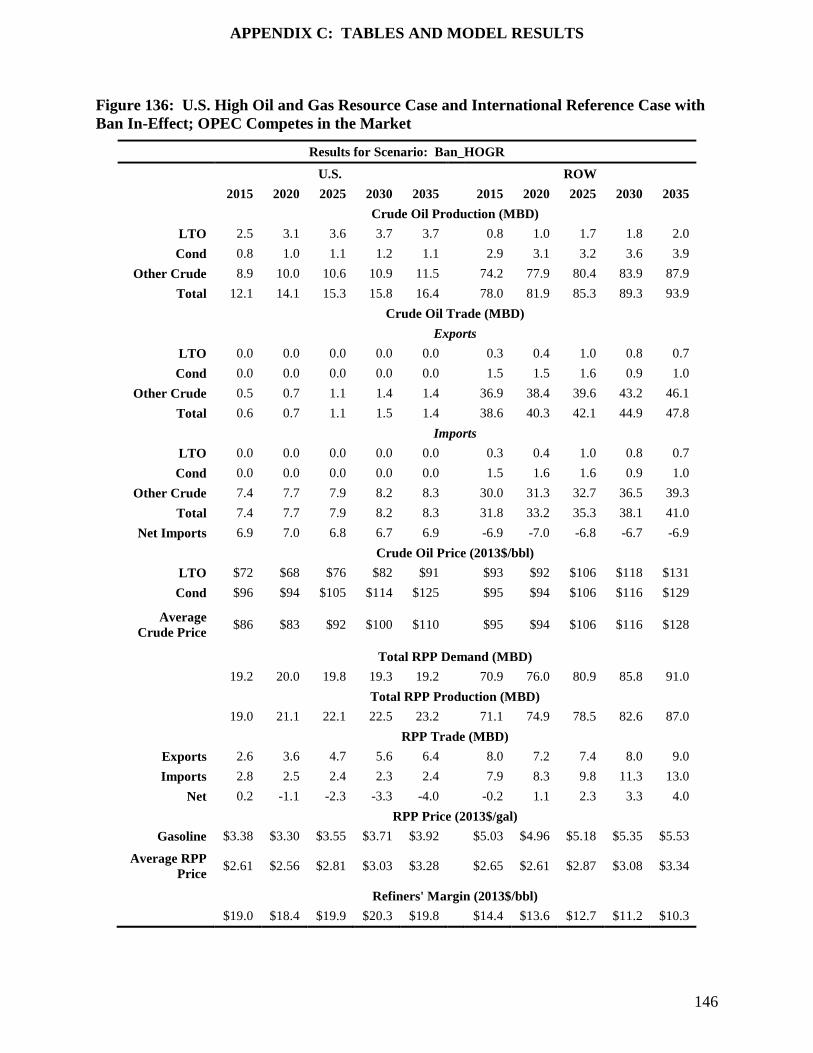
APPENDIX C: TABLES AND MODEL RESULTS
146
Figure 136: U.S. High Oil and Gas Resource Case and International Reference Case with Ban In-Effect; OPEC Competes in the Market
Results for Scenario: Ban_HOGR
U.S. ROW
2015 2020 2025 2030 2035 2015 2020 2025 2030 2035
Crude Oil Production (MBD) LTO 2.5 3.1 3.6 3.7 3.7 0.8 1.0 1.7 1.8 2.0 Cond 0.8 1.0 1.1 1.2 1.1 2.9 3.1 3.2 3.6 3.9
Other Crude 8.9 10.0 10.6 10.9 11.5 74.2 77.9 80.4 83.9 87.9 Total 12.1 14.1 15.3 15.8 16.4 78.0 81.9 85.3 89.3 93.9
Crude Oil Trade (MBD)
Exports LTO 0.0 0.0 0.0 0.0 0.0 0.3 0.4 1.0 0.8 0.7 Cond 0.0 0.0 0.0 0.0 0.0 1.5 1.5 1.6 0.9 1.0
Other Crude 0.5 0.7 1.1 1.4 1.4 36.9 38.4 39.6 43.2 46.1 Total 0.6 0.7 1.1 1.5 1.4 38.6 40.3 42.1 44.9 47.8
Imports LTO 0.0 0.0 0.0 0.0 0.0 0.3 0.4 1.0 0.8 0.7 Cond 0.0 0.0 0.0 0.0 0.0 1.5 1.6 1.6 0.9 1.0
Other Crude 7.4 7.7 7.9 8.2 8.3 30.0 31.3 32.7 36.5 39.3 Total 7.4 7.7 7.9 8.2 8.3 31.8 33.2 35.3 38.1 41.0
Net Imports 6.9 7.0 6.8 6.7 6.9 -6.9 -7.0 -6.8 -6.7 -6.9
Crude Oil Price (2013$/bbl) LTO $72 $68 $76 $82 $91 $93 $92 $106 $118 $131 Cond $96 $94 $105 $114 $125 $95 $94 $106 $116 $129
Average Crude Price $86 $83 $92 $100 $110 $95 $94 $106 $116 $128
Total RPP Demand (MBD)
19.2 20.0 19.8 19.3 19.2 70.9 76.0 80.9 85.8 91.0
Total RPP Production (MBD)
19.0 21.1 22.1 22.5 23.2 71.1 74.9 78.5 82.6 87.0
RPP Trade (MBD) Exports 2.6 3.6 4.7 5.6 6.4 8.0 7.2 7.4 8.0 9.0 Imports 2.8 2.5 2.4 2.3 2.4 7.9 8.3 9.8 11.3 13.0
Net 0.2 -1.1 -2.3 -3.3 -4.0 -0.2 1.1 2.3 3.3 4.0
RPP Price (2013$/gal) Gasoline $3.38 $3.30 $3.55 $3.71 $3.92 $5.03 $4.96 $5.18 $5.35 $5.53
Average RPP Price $2.61 $2.56 $2.81 $3.03 $3.28 $2.65 $2.61 $2.87 $3.08 $3.34
Refiners' Margin (2013$/bbl) $19.0 $18.4 $19.9 $20.3 $19.8 $14.4 $13.6 $12.7 $11.2 $10.3

APPENDIX C: TABLES AND MODEL RESULTS
147
Figure 137: U.S. High Oil and Gas Resource Case and International Reference Case with Crude Oil Ban Lifted in 2015; OPEC Competes in the Market
Results for Scenario: NoBan_HOGR
U.S. ROW
2015 2020 2025 2030 2035 2015 2020 2025 2030 2035
Crude Oil Production (MBD) LTO 4.3 5.6 6.7 7.0 7.4 0.8 0.9 1.6 1.7 2.0 Cond 1.2 1.4 1.7 1.8 1.9 2.9 3.0 3.1 3.5 3.8
Other Crude 8.7 9.9 10.4 10.8 11.4 72.8 76.1 78.3 81.5 85.4 Total 14.2 16.9 18.8 19.6 20.6 76.4 80.0 83.1 86.7 91.1
Crude Oil Trade (MBD)
Exports LTO 1.9 2.9 2.9 3.3 3.6 0.3 0.4 1.0 0.7 0.7 Cond 0.9 0.8 1.2 1.2 1.3 1.4 1.5 1.3 0.8 0.9
Other Crude 0.3 0.5 1.1 1.6 1.8 35.8 37.3 38.4 41.3 44.1 Total 3.1 4.2 5.3 6.0 6.7 37.5 39.1 40.7 42.8 45.6
Imports LTO 0.0 0.0 0.0 0.0 0.0 2.1 3.2 3.9 4.0 4.3 Cond 0.0 0.0 0.0 0.0 0.0 2.3 2.3 2.5 2.0 2.2
Other Crude 7.8 8.2 8.6 8.8 9.0 28.3 29.5 31.0 34.1 36.9 Total 7.8 8.3 8.6 8.8 9.0 32.7 35.1 37.4 40.0 43.3
Net Imports 4.7 4.0 3.3 2.8 2.3 -4.7 -4.0 -3.3 -2.8 -2.3
Crude Oil Price (2013$/bbl) LTO $86 $85 $97 $107 $118 $86 $86 $100 $111 $123 Cond $91 $91 $100 $109 $120 $89 $89 $100 $110 $122
Average Crude Price $88 $87 $98 $108 $119 $89 $89 $100 $109 $121
Total RPP Demand (MBD)
19.3 20.1 20.0 19.5 19.4 71.4 76.8 81.9 86.8 92.3
Total RPP Production (MBD)
19.0 21.0 22.1 22.4 22.9 71.7 76.0 79.7 83.9 88.8
RPP Trade (MBD) Exports 2.5 3.3 4.4 5.2 5.9 8.3 8.1 7.7 8.8 9.9 Imports 2.8 2.5 2.3 2.3 2.5 8.0 8.9 9.8 11.7 13.4
Net 0.3 -0.8 -2.1 -2.9 -3.5 -0.3 0.8 2.1 2.9 3.5
RPP Price (2013$/gal) Gasoline $3.25 $3.20 $3.45 $3.64 $3.84 $4.89 $4.85 $5.08 $5.27 $5.43
Average RPP Price $2.49 $2.45 $2.71 $2.93 $3.18 $2.53 $2.51 $2.77 $2.99 $3.24
Refiners' Margin (2013$/bbl) $14.7 $13.4 $13.7 $13.8 $12.9 $15.3 $14.6 $14.3 $13.8 $13.1

APPENDIX C: TABLES AND MODEL RESULTS
148
Figure 138: U.S. High Oil and Gas Resource Case and International Reference Case with Crude Oil Ban Lifted in 2020; OPEC Competes in the Market
Results for Scenario: NoBanDelay_HOGR
U.S. ROW
2015 2020 2025 2030 2035 2015 2020 2025 2030 2035
Crude Oil Production (MBD) LTO 2.5 5.6 6.7 7.0 7.4 0.8 0.9 1.6 1.7 2.0 Cond 0.8 1.4 1.7 1.8 1.9 2.9 3.0 3.1 3.5 3.8
Other Crude 8.9 9.9 10.4 10.8 11.4 74.2 76.1 78.3 81.5 85.4 Total 12.1 16.9 18.8 19.6 20.6 78.0 80.0 83.1 86.7 91.1
Crude Oil Trade (MBD)
Exports LTO 0.0 2.9 2.9 3.2 3.6 0.3 0.4 1.0 0.7 0.7 Cond 0.0 0.8 1.2 1.2 1.3 1.5 1.5 1.3 0.8 0.9
Other Crude 0.5 0.5 1.1 1.6 1.8 36.9 37.3 38.4 41.3 44.1 Total 0.6 4.2 5.3 6.0 6.7 38.6 39.1 40.7 42.8 45.6
Imports LTO 0.0 0.0 0.0 0.0 0.0 0.3 3.2 3.9 4.0 4.3 Cond 0.0 0.0 0.0 0.0 0.0 1.5 2.3 2.5 2.0 2.2
Other Crude 7.4 8.2 8.6 8.8 9.0 30.0 29.6 31.0 34.1 36.9 Total 7.4 8.3 8.6 8.8 9.0 31.8 35.1 37.4 40.0 43.3
Net Imports 6.9 4.0 3.3 2.8 2.3 -6.9 -4.0 -3.3 -2.8 -2.3
Crude Oil Price (2013$/bbl) LTO $72 $85 $97 $107 $118 $93 $86 $100 $111 $123 Cond $96 $91 $100 $109 $120 $95 $89 $100 $110 $122
Average Crude Price $86 $87 $98 $108 $119 $95 $89 $100 $109 $121
Total RPP Demand (MBD)
19.2 20.1 20.0 19.5 19.4 70.9 76.8 81.9 86.8 92.3
Total RPP Production (MBD)
19.0 21.0 22.1 22.4 22.9 71.1 76.0 79.7 83.9 88.8
RPP Trade (MBD) Exports 2.6 3.3 4.4 5.2 5.9 8.0 8.1 7.7 8.8 9.9 Imports 2.8 2.5 2.3 2.3 2.5 7.9 8.9 9.8 11.7 13.4
Net 0.2 -0.8 -2.1 -2.9 -3.5 -0.2 0.8 2.1 2.9 3.5
RPP Price (2013$/gal) Gasoline $3.38 $3.20 $3.45 $3.64 $3.84 $5.03 $4.85 $5.08 $5.27 $5.43
Average RPP Price $2.61 $2.45 $2.71 $2.93 $3.18 $2.65 $2.51 $2.77 $2.99 $3.24
Refiners' Margin (2013$/bbl) $19.0 $13.4 $13.7 $13.8 $12.9 $14.4 $14.6 $14.3 $13.8 $13.1

APPENDIX C: TABLES AND MODEL RESULTS
149
Figure 139: U.S. High Oil and Gas Resource Case and International Reference Case with Condensate Ban Lifted in 2015; OPEC Competes in the Market
Results for Scenario: NoBanCond_HOGR
U.S. ROW
2015 2020 2025 2030 2035 2015 2020 2025 2030 2035
Crude Oil Production (MBD) LTO 3.0 3.8 4.5 4.6 4.7 0.8 0.9 1.7 1.7 2.0 Cond 1.2 1.4 1.6 1.7 1.7 2.9 3.1 3.2 3.6 3.9
Other Crude 8.8 9.9 10.5 10.9 11.5 73.6 77.2 79.6 83.2 87.0 Total 13.0 15.1 16.5 17.2 17.8 77.3 81.2 84.4 88.5 92.9
Crude Oil Trade (MBD)
Exports LTO 0.0 0.0 0.0 0.0 0.0 0.3 0.4 1.0 0.7 0.7 Cond 1.0 1.1 1.4 1.5 1.6 1.4 1.5 1.4 0.8 0.9
Other Crude 0.5 0.7 1.1 1.4 1.4 36.3 38.1 39.3 42.8 45.7 Total 1.5 1.8 2.5 2.9 3.0 38.0 40.0 41.7 44.3 47.3
Imports LTO 0.0 0.0 0.0 0.0 0.0 0.3 0.4 1.0 0.7 0.7 Cond 0.0 0.0 0.0 0.0 0.0 2.4 2.7 2.8 2.3 2.5
Other Crude 7.5 7.8 8.1 8.3 8.3 29.4 31.0 32.4 36.0 38.8 Total 7.5 7.8 8.1 8.3 8.3 32.0 34.0 36.1 39.0 42.0
Net Imports 6.0 6.0 5.6 5.4 5.4 -6.0 -6.0 -5.6 -5.4 -5.4
Crude Oil Price (2013$/bbl) LTO $75 $71 $79 $86 $94 $86 $86 $102 $114 $127 Cond $94 $92 $102 $112 $124 $92 $92 $104 $115 $126
Average Crude Price $86 $84 $92 $101 $111 $93 $92 $103 $114 $125
Total RPP Demand (MBD)
19.2 20.0 19.8 19.4 19.3 71.1 76.2 81.1 86.3 91.5
Total RPP Production (MBD)
19.0 21.1 22.1 22.5 23.2 71.4 75.2 78.8 83.1 87.6
RPP Trade (MBD) Exports 2.6 3.6 4.6 5.3 6.0 8.2 7.6 7.5 8.3 9.3 Imports 2.8 2.5 2.3 2.1 2.1 7.9 8.6 9.8 11.4 13.2
Net 0.2 -1.0 -2.3 -3.2 -3.9 -0.2 1.0 2.3 3.2 3.9
RPP Price (2013$/gal) Gasoline $3.32 $3.27 $3.52 $3.67 $3.88 $4.96 $4.92 $5.16 $5.30 $5.48
Average RPP Price $2.55 $2.52 $2.79 $2.99 $3.24 $2.59 $2.58 $2.84 $3.04 $3.30
Refiners' Margin (2013$/bbl) $17.3 $17.6 $19.8 $19.1 $18.5 $14.5 $14.3 $14.2 $11.8 $11.3

APPENDIX C: TABLES AND MODEL RESULTS
150
Figure 140: U.S. High Oil and Gas Resource Case and International Reference Case with Crude Oil Ban Lifted in 2015; OPEC Maintains Crude Oil Exports
Results for Scenario: NoBanOPECFix_HOGR
U.S. ROW
2015 2020 2025 2030 2035 2015 2020 2025 2030 2035
Crude Oil Production (MBD) LTO 4.3 5.6 6.7 7.0 7.4 0.8 0.9 1.6 1.7 1.9 Cond 1.2 1.4 1.7 1.8 1.9 2.9 3.0 3.1 3.5 3.8
Other Crude 8.7 9.9 10.4 10.8 11.4 72.8 76.1 78.4 81.6 85.4 Total 14.2 16.9 18.7 19.6 20.6 76.4 80.1 83.1 86.8 91.2
Crude Oil Trade (MBD)
Exports LTO 1.9 2.9 2.9 3.2 3.6 0.3 0.4 1.0 0.7 0.7 Cond 0.8 0.8 1.2 1.2 1.3 1.4 1.5 1.4 0.8 0.9
Other Crude 0.3 0.5 1.1 1.5 1.8 36.1 37.8 39.0 42.1 44.9 Total 3.1 4.2 5.2 5.9 6.7 37.8 39.6 41.3 43.6 46.5
Imports LTO 0.1 0.0 0.0 0.0 0.0 2.2 3.2 3.9 3.9 4.3 Cond 0.0 0.0 0.0 0.0 0.0 2.3 2.3 2.6 2.0 2.1
Other Crude 7.8 8.3 8.6 8.8 9.0 28.6 30.0 31.6 34.9 37.7 Total 7.8 8.3 8.6 8.8 9.0 33.1 35.6 38.0 40.8 44.1
Net Imports 4.8 4.1 3.4 2.9 2.3 -4.8 -4.1 -3.4 -2.9 -2.3
Crude Oil Price (2013$/bbl) LTO $85 $85 $96 $106 $118 $86 $86 $100 $111 $122 Cond $90 $90 $100 $109 $119 $90 $90 $101 $111 $122
Average Crude Price $88 $87 $98 $107 $119 $89 $89 $100 $109 $121
Total RPP Demand (MBD)
19.3 20.2 20.0 19.5 19.5 71.4 76.8 81.9 86.9 92.3
Total RPP Production (MBD)
19.0 21.0 22.1 22.4 22.9 71.7 76.0 79.8 83.9 88.9
RPP Trade (MBD) Exports 2.5 3.3 4.4 5.2 5.9 8.2 8.0 7.7 8.7 9.9 Imports 2.8 2.5 2.3 2.3 2.5 7.9 8.9 9.8 11.6 13.3
Net 0.3 -0.8 -2.1 -2.9 -3.5 -0.3 0.8 2.1 2.9 3.5
RPP Price (2013$/gal) Gasoline $3.25 $3.19 $3.45 $3.64 $3.83 $4.89 $4.84 $5.07 $5.27 $5.42
Average RPP Price $2.49 $2.44 $2.71 $2.93 $3.18 $2.53 $2.50 $2.77 $2.99 $3.24
Refiners' Margin (2013$/bbl) $15.0 $13.4 $13.7 $14.0 $13.0 $15.2 $14.1 $13.9 $13.5 $12.6

APPENDIX C: TABLES AND MODEL RESULTS
151
Figure 141: U.S. High Oil and Gas Resource Case and International Reference Case with Crude Oil Ban Lifted in 2015; OPEC Cuts Crude Oil Exports to Maintain Price
Results for Scenario: NoBanOPECCut_HOGR
U.S. ROW
2015 2020 2025 2030 2035 2015 2020 2025 2030 2035
Crude Oil Production (MBD) LTO 4.6 5.9 6.9 7.2 7.6 0.8 1.0 1.7 1.7 2.0 Cond 1.3 1.5 1.7 1.8 1.9 2.8 2.9 3.0 3.4 3.7
Other Crude 8.9 10.0 10.6 11.0 11.6 71.8 74.9 76.9 80.2 83.7 Total 14.8 17.4 19.2 20.0 21.1 75.4 78.8 81.6 85.3 89.3
Crude Oil Trade (MBD)
Exports LTO 2.1 2.9 3.2 3.6 3.9 0.3 0.4 1.0 0.7 0.7 Cond 0.9 1.0 1.2 1.2 1.4 1.3 1.4 1.3 0.8 0.9
Other Crude 0.3 0.7 1.1 1.5 1.8 34.4 35.7 36.5 39.4 41.8 Total 3.4 4.6 5.6 6.3 7.1 36.0 37.5 38.8 41.0 43.4
Imports LTO 0.0 0.0 0.0 0.0 0.0 2.4 3.3 4.2 4.4 4.7 Cond 0.0 0.0 0.0 0.0 0.0 2.3 2.4 2.6 2.0 2.3
Other Crude 7.6 8.2 8.5 8.6 8.8 27.0 28.1 29.2 32.3 34.8 Total 7.6 8.3 8.5 8.6 8.8 31.7 33.8 35.9 38.7 41.7
Net Imports 4.3 3.7 2.9 2.3 1.7 -4.3 -3.7 -2.9 -2.3 -1.7
Crude Oil Price (2013$/bbl) LTO $91 $89 $100 $112 $124 $92 $90 $104 $116 $128 Cond $96 $94 $104 $113 $125 $93 $95 $106 $114 $125
Average Crude Price $93 $92 $102 $112 $124 $94 $94 $104 $113 $125
Total RPP Demand (MBD)
19.2 20.0 19.8 19.3 19.2 71.0 76.1 81.0 86.0 91.2
Total RPP Production (MBD)
19.0 21.1 22.1 22.3 22.7 71.1 75.0 78.7 83.1 87.7
RPP Trade (MBD) Exports 2.6 3.5 4.5 5.1 5.8 8.0 7.5 7.5 8.3 9.4 Imports 2.8 2.5 2.3 2.1 2.3 7.8 8.5 9.8 11.3 12.9
Net 0.2 -1.1 -2.3 -3.0 -3.5 -0.2 1.1 2.3 3.0 3.5
RPP Price (2013$/gal) Gasoline $3.37 $3.28 $3.53 $3.68 $3.91 $5.02 $4.94 $5.17 $5.32 $5.51
Average RPP Price $2.61 $2.54 $2.80 $3.01 $3.27 $2.65 $2.59 $2.85 $3.06 $3.32
Refiners' Margin (2013$/bbl) $14.2 $13.2 $13.6 $12.2 $11.3 $15.6 $13.3 $13.2 $12.5 $12.3

APPENDIX C: TABLES AND MODEL RESULTS
152
Figure 142: U.S. High Oil and Gas Resource Case and Low Asia-Pacific Demand Case with Ban In-Effect; OPEC Competes in the Market
Results for Scenario: BanLowAP_HOGR
U.S. ROW
2015 2020 2025 2030 2035 2015 2020 2025 2030 2035
Crude Oil Production (MBD) LTO 2.5 3.1 3.6 3.7 3.7 0.8 0.9 1.7 1.7 2.0 Cond 0.8 1.0 1.1 1.2 1.1 2.9 3.1 3.2 3.5 3.8
Other Crude 8.9 9.9 10.3 10.6 11.2 74.2 77.0 78.8 81.3 85.0 Total 12.1 14.0 15.1 15.5 16.1 78.0 81.0 83.6 86.5 90.8
Crude Oil Trade (MBD)
Exports LTO 0.0 0.0 0.0 0.0 0.0 0.3 0.3 1.0 0.7 0.7 Cond 0.0 0.0 0.0 0.0 0.0 1.5 2.1 2.2 0.9 1.0
Other Crude 0.5 0.7 1.0 1.4 1.4 36.9 36.9 37.6 41.3 44.8 Total 0.6 0.7 1.0 1.4 1.4 38.6 39.4 40.8 42.9 46.4
Imports LTO 0.0 0.0 0.0 0.0 0.0 0.3 0.3 1.0 0.7 0.7 Cond 0.0 0.0 0.0 0.0 0.0 1.5 2.1 2.2 0.9 1.0
Other Crude 7.4 7.8 8.0 8.4 8.4 30.0 29.8 30.6 34.4 37.7 Total 7.4 7.8 8.0 8.4 8.4 31.8 32.3 33.8 35.9 39.4
Net Imports 6.9 7.1 7.0 6.9 7.0 -6.9 -7.1 -7.0 -6.9 -7.0
Crude Oil Price (2013$/bbl) LTO $72 $68 $76 $83 $91 $93 $89 $103 $112 $124 Cond $96 $92 $101 $109 $119 $95 $92 $102 $111 $122
Average Crude Price $86 $82 $90 $97 $106 $95 $92 $102 $110 $121
Total RPP Demand (MBD)
19.2 20.1 20.0 19.7 19.6 70.9 74.9 78.6 82.3 87.2
Total RPP Production (MBD)
19.0 21.1 22.0 22.4 23.1 71.1 73.9 76.6 79.6 83.8
RPP Trade (MBD) Exports 2.6 3.5 4.4 4.7 5.5 8.0 6.4 6.4 7.2 7.6 Imports 2.8 2.6 2.4 2.0 2.0 7.9 7.4 8.4 9.9 11.1
Net 0.2 -1.0 -2.0 -2.7 -3.5 -0.2 1.0 2.0 2.7 3.5
RPP Price (2013$/gal) Gasoline $3.38 $3.24 $3.39 $3.55 $3.76 $5.03 $4.88 $5.03 $5.19 $5.36
Average RPP Price $2.61 $2.49 $2.69 $2.87 $3.12 $2.65 $2.54 $2.72 $2.89 $3.13
Refiners' Margin (2013$/bbl) $19.0 $17.3 $16.8 $17.2 $17.3 $14.4 $12.8 $10.3 $8.9 $8.7

APPENDIX C: TABLES AND MODEL RESULTS
153
Figure 143: U.S. High Oil and Gas Resource Case and Low Asia-Pacific Demand Case with Crude Oil Ban Lifted in 2015; OPEC Competes in the Market
Results for Scenario: NoBanLowAP_HOGR
U.S. ROW
2015 2020 2025 2030 2035 2015 2020 2025 2030 2035
Crude Oil Production (MBD) LTO 4.3 5.5 6.5 6.9 7.2 0.8 0.9 1.6 1.7 1.9 Cond 1.2 1.4 1.7 1.7 1.8 2.9 3.0 3.1 3.4 3.7
Other Crude 8.7 9.8 10.2 10.5 11.0 72.8 75.4 76.7 79.2 83.0 Total 14.2 16.7 18.3 19.1 20.1 76.4 79.3 81.4 84.3 88.6
Crude Oil Trade (MBD)
Exports LTO 1.9 2.6 2.9 3.1 3.6 0.3 0.4 0.9 0.7 0.7 Cond 0.9 1.0 1.2 1.2 1.3 1.4 1.9 2.1 1.6 0.8
Other Crude 0.3 0.5 1.0 1.3 1.6 35.8 36.1 36.2 38.6 42.4 Total 3.1 4.0 5.0 5.7 6.4 37.5 38.4 39.2 40.9 43.9
Imports LTO 0.0 0.0 0.0 0.0 0.0 2.1 3.0 3.8 3.8 4.2 Cond 0.0 0.0 0.0 0.0 0.0 2.3 2.9 3.3 2.8 2.1
Other Crude 7.8 8.3 8.3 8.7 8.7 28.3 28.2 28.9 31.3 35.2 Total 7.8 8.4 8.3 8.7 8.7 32.7 34.1 36.0 37.9 41.6
Net Imports 4.7 4.3 3.3 3.0 2.3 -4.7 -4.3 -3.3 -3.0 -2.3
Crude Oil Price (2013$/bbl) LTO $86 $83 $93 $102 $113 $86 $84 $97 $107 $118 Cond $91 $89 $97 $105 $115 $89 $87 $97 $106 $117
Average Crude Price $88 $86 $94 $103 $114 $89 $87 $96 $105 $116
Total RPP Demand (MBD)
19.3 20.2 20.2 19.9 19.9 71.4 75.8 79.5 83.5 88.8
Total RPP Production (MBD)
19.0 21.0 21.6 22.1 22.4 71.7 75.0 78.1 81.3 86.3
RPP Trade (MBD) Exports 2.5 3.5 3.7 4.3 4.6 8.3 6.7 7.0 7.5 7.9 Imports 2.8 2.7 2.3 2.1 2.0 8.0 7.5 8.4 9.7 10.4
Net 0.3 -0.8 -1.4 -2.2 -2.5 -0.3 0.8 1.4 2.2 2.5
RPP Price (2013$/gal) Gasoline $3.25 $3.14 $3.33 $3.46 $3.66 $4.89 $4.77 $4.95 $5.07 $5.24
Average RPP Price $2.49 $2.39 $2.61 $2.79 $3.03 $2.53 $2.44 $2.63 $2.80 $3.03
Refiners' Margin (2013$/bbl) $14.7 $12.6 $12.9 $12.1 $10.8 $15.3 $13.8 $12.3 $10.3 $9.2

APPENDIX C: TABLES AND MODEL RESULTS
154
Figure 144: U.S. and International Low Oil Price Cases with Ban In-Effect; OPEC Competes in the Market
Results for Scenario: Ban_LOP
U.S. ROW
2015 2020 2025 2030 2035 2015 2020 2025 2030 2035
Crude Oil Production (MBD) LTO 1.9 1.7 0.9 0.6 0.3 0.8 1.0 1.7 1.8 2.1 Cond 0.6 0.6 0.4 0.2 0.1 3.3 3.7 4.1 4.7 5.1
Other Crude 8.6 9.3 9.3 8.9 8.7 75.1 80.9 87.7 94.2 100.1 Total 11.2 11.6 10.6 9.7 9.1 79.2 85.6 93.6 100.7 107.3
Crude Oil Trade (MBD)
Exports LTO 0.0 0.0 0.0 0.0 0.0 0.3 0.6 1.2 1.2 1.1 Cond 0.0 0.0 0.0 0.0 0.0 1.6 2.8 3.1 2.6 1.7
Other Crude 0.4 0.5 0.5 0.4 0.4 35.9 39.4 44.2 49.8 55.7 Total 0.4 0.5 0.5 0.4 0.4 37.8 42.8 48.5 53.7 58.4
Imports LTO 0.2 0.4 0.6 0.5 0.7 0.2 0.2 0.6 0.7 0.4 Cond 0.0 0.6 0.9 1.1 1.1 1.6 2.2 2.3 1.5 0.6
Other Crude 8.0 8.3 9.8 10.4 10.8 28.3 31.6 34.9 39.9 45.2 Total 8.2 9.4 11.3 12.0 12.6 30.0 33.9 37.8 42.1 46.3
Net Imports 7.8 8.8 10.8 11.6 12.2 -7.8 -8.8 -10.8 -11.6 -12.2
Crude Oil Price (2013$/bbl) LTO $70 $67 $75 $78 $78 $69 $63 $69 $73 $75 Cond $74 $69 $70 $71 $73 $72 $66 $68 $70 $71
Average Crude Price $72 $68 $71 $72 $73 $72 $65 $68 $69 $70
Total RPP Demand (MBD)
16.5 17.2 17.2 17.0 17.0 73.9 79.9 86.9 93.4 99.4
Total RPP Production (MBD)
19.0 20.5 21.3 21.2 21.3 71.4 76.7 82.8 89.2 95.1
RPP Trade (MBD) Exports 4.5 4.9 6.0 6.0 6.1 6.4 7.4 7.7 8.2 10.0 Imports 2.0 1.7 1.9 1.8 1.8 8.8 10.6 11.9 12.5 14.3
Net -2.4 -3.2 -4.1 -4.3 -4.3 2.4 3.2 4.1 4.3 4.3
RPP Price (2013$/gal) Gasoline $2.77 $2.66 $2.63 $2.64 $2.68 $4.63 $4.54 $4.49 $4.51 $4.53
Average RPP Price $2.15 $2.05 $2.04 $2.05 $2.10 $2.20 $2.12 $2.11 $2.11 $2.16
Refiners' Margin (2013$/bbl) $17.7 $18.8 $15.9 $15.8 $16.7 $18.8 $21.3 $18.5 $17.1 $17.6
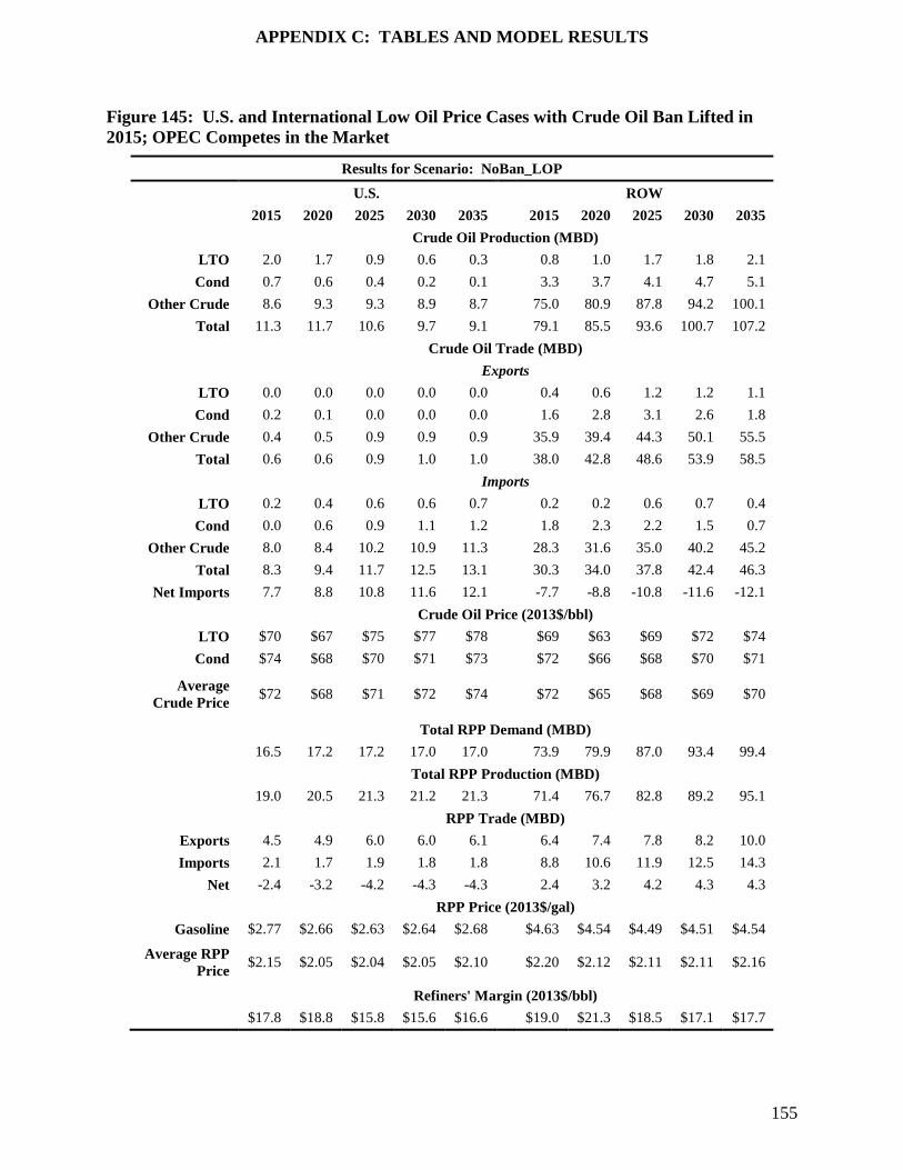
APPENDIX C: TABLES AND MODEL RESULTS
155
Figure 145: U.S. and International Low Oil Price Cases with Crude Oil Ban Lifted in 2015; OPEC Competes in the Market
Results for Scenario: NoBan_LOP
U.S. ROW
2015 2020 2025 2030 2035 2015 2020 2025 2030 2035
Crude Oil Production (MBD) LTO 2.0 1.7 0.9 0.6 0.3 0.8 1.0 1.7 1.8 2.1 Cond 0.7 0.6 0.4 0.2 0.1 3.3 3.7 4.1 4.7 5.1
Other Crude 8.6 9.3 9.3 8.9 8.7 75.0 80.9 87.8 94.2 100.1 Total 11.3 11.7 10.6 9.7 9.1 79.1 85.5 93.6 100.7 107.2
Crude Oil Trade (MBD)
Exports LTO 0.0 0.0 0.0 0.0 0.0 0.4 0.6 1.2 1.2 1.1 Cond 0.2 0.1 0.0 0.0 0.0 1.6 2.8 3.1 2.6 1.8
Other Crude 0.4 0.5 0.9 0.9 0.9 35.9 39.4 44.3 50.1 55.5 Total 0.6 0.6 0.9 1.0 1.0 38.0 42.8 48.6 53.9 58.5
Imports LTO 0.2 0.4 0.6 0.6 0.7 0.2 0.2 0.6 0.7 0.4 Cond 0.0 0.6 0.9 1.1 1.2 1.8 2.3 2.2 1.5 0.7
Other Crude 8.0 8.4 10.2 10.9 11.3 28.3 31.6 35.0 40.2 45.2 Total 8.3 9.4 11.7 12.5 13.1 30.3 34.0 37.8 42.4 46.3
Net Imports 7.7 8.8 10.8 11.6 12.1 -7.7 -8.8 -10.8 -11.6 -12.1
Crude Oil Price (2013$/bbl) LTO $70 $67 $75 $77 $78 $69 $63 $69 $72 $74 Cond $74 $68 $70 $71 $73 $72 $66 $68 $70 $71
Average Crude Price $72 $68 $71 $72 $74 $72 $65 $68 $69 $70
Total RPP Demand (MBD)
16.5 17.2 17.2 17.0 17.0 73.9 79.9 87.0 93.4 99.4
Total RPP Production (MBD)
19.0 20.5 21.3 21.2 21.3 71.4 76.7 82.8 89.2 95.1
RPP Trade (MBD) Exports 4.5 4.9 6.0 6.0 6.1 6.4 7.4 7.8 8.2 10.0 Imports 2.1 1.7 1.9 1.8 1.8 8.8 10.6 11.9 12.5 14.3
Net -2.4 -3.2 -4.2 -4.3 -4.3 2.4 3.2 4.2 4.3 4.3
RPP Price (2013$/gal) Gasoline $2.77 $2.66 $2.63 $2.64 $2.68 $4.63 $4.54 $4.49 $4.51 $4.54
Average RPP Price $2.15 $2.05 $2.04 $2.05 $2.10 $2.20 $2.12 $2.11 $2.11 $2.16
Refiners' Margin (2013$/bbl) $17.8 $18.8 $15.8 $15.6 $16.6 $19.0 $21.3 $18.5 $17.1 $17.7

APPENDIX C: TABLES AND MODEL RESULTS
156
B. NewERA Model Results
The following figures present detailed results from the NewERA Model for each of the 16 scenarios run as part of this study. The table below provides an explanation of selected abbreviations that appear in the figures. NewERA Macroeconomic Model Acronyms and Abbreviations NPV Net Present Value
CAGR Compound Annual Growth Rate
Avg 15-20
Average of the years between 2015 and 2020
Figure 146: U.S. and International Reference Cases with Ban In-Effect; OPEC Competes in the Market
Results for Scenario: Ban_Ref
2015 2020 2025 2030 2035 CAGR GDP Billion $
16,360 18,661 20,900 23,535 26,391 2.4%
Consumption Billion $
12,314 13,936 15,482 17,360 19,415 2.3% Investment Billion $
2,282 2,873 3,305 3,690 4,117
Wage Income Billion $
8,026 9,196 10,303 11,639 13,079 Capital Income Billion $
3,723 4,236 4,707 5,251 5,821
Resource & Sector-specific Capital Income Billion $
181 165 249 311 425
Total Emissions MMTCO2 11,502 11,693 11,826 11,803 11,764

APPENDIX C: TABLES AND MODEL RESULTS
157
Figure 147: U.S. and International Reference Cases with Crude Oil Export Ban Lifted in 2015; OPEC Competes in the Market 52
Results for Scenario: NoBan_Ref
Avg 15-20 2015 2020 2025 2030 2035 DNPV Welfare %
0.3 0.1 0.1 0.1 0.1
Billion $
41.5 24.4 20.4 22.3 22.0 460.9 GDP %
0.4 0.2 0.1 0.0 0.0
Billion $
66.0 39.2 14.9 8.3 3.7 556.1 Consumption %
0.3 0.1 0.1 0.1 0.1
Billion $
35.5 20.5 16.8 18.3 18.0 387.3 Investment %
1.0 -0.2 -0.2 0.1 0.0
Billion $
23.4 -6.6 -6.1 2.1 1.7 Wage Income %
0.5 0.1 0.0 0.0 0.0
Billion $
40.7 10.9 -1.7 0.7 -0.4 Capital Income %
-0.1 0.1 0.0 0.0 0.0
Billion $
-2.9 5.2 1.4 -1.6 -1.4
Resource & Sector-specific Capital Income %
2.8 11.1 6.1 3.4 1.5
Billion $
5.0 18.3 15.2 10.7 6.4
Change in Industrial and service sectoral output %
0.0 0.1 0.0 0.0 0.0
Reduction in Unemployment (Annual average) Thousands 229
Change in Total Emissions MMTCO2 26.2 17.1 6.8 8.6 4.7
52 All NewERA NoBan scenarios show changes from baseline (corresponding ban) in Billion $, % or MMTCO2.

APPENDIX C: TABLES AND MODEL RESULTS
158
Figure 148: U.S. and International Reference Cases with Crude Oil Export Ban Lifted in 2020; OPEC Competes in the Market 53
Results for Scenario: NoBanDelay_Ref
Avg 15-20 2015 2020 2025 2030 2035 DNPV Welfare %
0.0 0.1 0.1 0.1 0.1
Billion $
5.8 11.9 12.0 14.0 13.0 170.8 GDP %
0.0 0.2 0.1 0.0 0.0
Billion $
2.7 33.1 14.6 10.2 6.6 225.1 Consumption %
0.0 0.1 0.1 0.1 0.1
Billion $
4.8 10.1 9.9 11.6 10.7 141.8 Investment %
0.1 0.1 -0.1 0.1 0.1
Billion $
2.8 2.4 -3.8 3.0 2.8 Wage Income %
0.0 0.1 0.0 0.0 0.0
Billion $
0.2 7.6 -1.9 1.5 0.9 Capital Income %
0.0 0.1 0.0 0.0 0.0
Billion $
-0.2 5.0 1.8 -0.9 -0.7
Resource & Sector-specific Capital Income %
0.0 10.6 6.1 3.5 1.6
Billion $
-0.1 17.5 15.3 10.8 6.8
Change in Industrial and service sectoral output %
0.0 0.0 0.0 0.1 0.0
Reduction in Unemployment (Annual average) Thousands 32
Change in Total Emissions MMTCO2 0.9 15.1 6.5 8.5 4.8
53 All NewERA NoBan scenarios show changes from baseline (corresponding ban) in Billion $, % or MMTCO2.
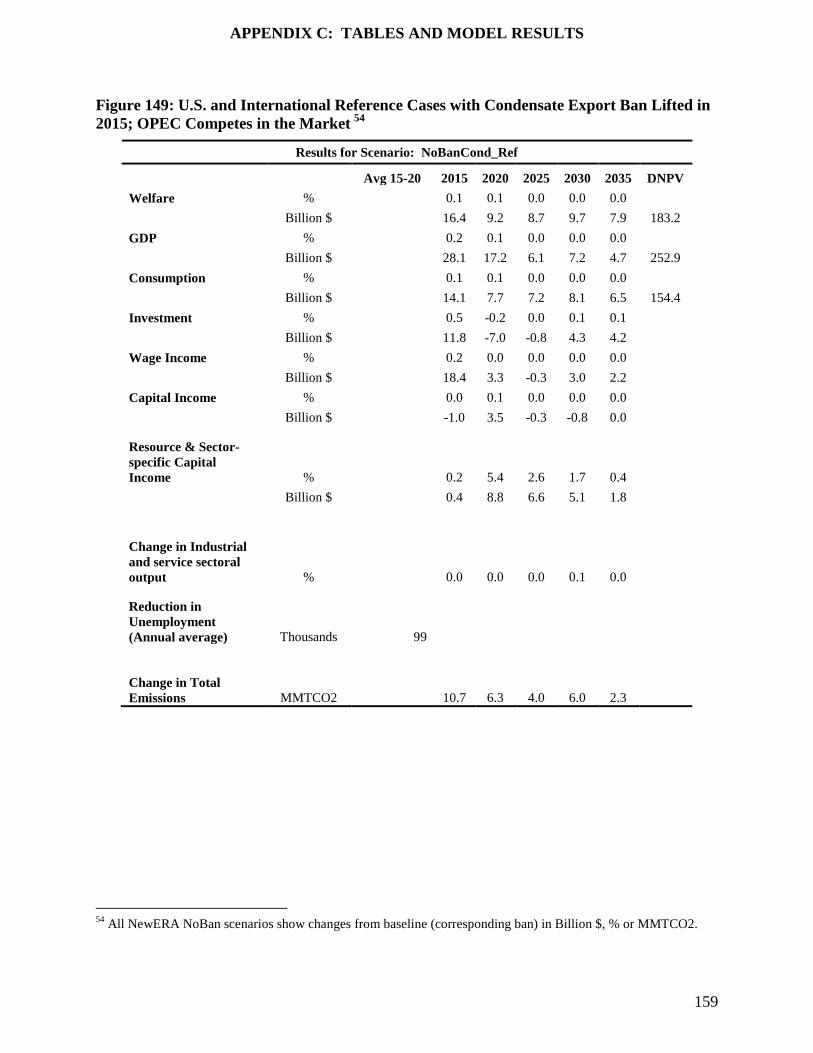
APPENDIX C: TABLES AND MODEL RESULTS
159
Figure 149: U.S. and International Reference Cases with Condensate Export Ban Lifted in 2015; OPEC Competes in the Market 54
Results for Scenario: NoBanCond_Ref
Avg 15-20 2015 2020 2025 2030 2035 DNPV Welfare %
0.1 0.1 0.0 0.0 0.0
Billion $
16.4 9.2 8.7 9.7 7.9 183.2 GDP %
0.2 0.1 0.0 0.0 0.0
Billion $
28.1 17.2 6.1 7.2 4.7 252.9 Consumption %
0.1 0.1 0.0 0.0 0.0
Billion $
14.1 7.7 7.2 8.1 6.5 154.4 Investment %
0.5 -0.2 0.0 0.1 0.1
Billion $
11.8 -7.0 -0.8 4.3 4.2 Wage Income %
0.2 0.0 0.0 0.0 0.0
Billion $
18.4 3.3 -0.3 3.0 2.2 Capital Income %
0.0 0.1 0.0 0.0 0.0
Billion $
-1.0 3.5 -0.3 -0.8 0.0
Resource & Sector-specific Capital Income %
0.2 5.4 2.6 1.7 0.4
Billion $
0.4 8.8 6.6 5.1 1.8
Change in Industrial and service sectoral output %
0.0 0.0 0.0 0.1 0.0
Reduction in Unemployment (Annual average) Thousands 99
Change in Total Emissions MMTCO2 10.7 6.3 4.0 6.0 2.3
54 All NewERA NoBan scenarios show changes from baseline (corresponding ban) in Billion $, % or MMTCO2.

APPENDIX C: TABLES AND MODEL RESULTS
160
Figure 150: U.S. and International Reference Cases with Crude Oil Export Ban Lifted in 2015; OPEC Maintains Crude Oil Exports 55
Results for Scenario: NoBanOPECFix_Ref
Avg 15-20 2015 2020 2025 2030 2035 DNPV Welfare %
0.3 0.2 0.1 0.1 0.1
Billion $
43.7 26.2 21.7 23.2 23.6 488.0 GDP %
0.4 0.2 0.1 0.0 0.0
Billion $
70.4 41.3 14.7 8.1 2.3 582.7 Consumption %
0.3 0.2 0.1 0.1 0.1
Billion $
37.3 22.0 17.9 19.1 19.3 410.2 Investment %
1.1 -0.2 -0.2 0.0 0.0
Billion $
24.7 -6.8 -5.6 0.9 0.5 Wage Income %
0.5 0.1 0.0 0.0 0.0
Billion $
43.6 13.0 -0.5 0.2 -0.9 Capital Income %
-0.1 0.1 0.0 0.0 0.0
Billion $
-2.4 5.6 1.2 -1.2 -1.6
Resource & Sector-specific Capital Income %
2.2 10.2 5.3 3.5 1.4
Billion $
3.9 16.7 13.2 10.8 6.1
Change in Industrial and service sectoral output %
0.0 0.1 0.0 0.0 0.0
Reduction in Unemployment (Annual average) Thousands 243
Change in Total Emissions MMTCO2 27.4 18.2 7.0 8.4 4.6
55 All NewERA NoBan scenarios show changes from baseline (corresponding ban) in Billion $, % or MMTCO2.

APPENDIX C: TABLES AND MODEL RESULTS
161
Figure 151: U.S. and International Reference Cases with Crude Oil Export Ban Lifted in 2015; OPEC Cuts Crude Oil Exports to Maintain Price 56
Results for Scenario: NoBanOPECCut_Ref
Avg 15-20 2015 2020 2025 2030 2035 DNPV Welfare %
0.1 0.1 0.1 0.1 0.0
Billion $
21.2 14.4 11.6 12.9 11.4 250.6 GDP %
0.1 0.1 0.1 0.0 0.0
Billion $
21.8 27.6 15.7 10.7 7.8 306.3 Consumption %
0.1 0.1 0.1 0.1 0.0
Billion $
17.8 12.0 9.5 10.7 9.4 208.7 Investment %
0.3 0.0 -0.1 0.1 0.1
Billion $
7.7 1.2 -4.9 2.9 2.6 Wage Income %
0.1 0.0 0.0 0.0 0.0
Billion $
7.4 2.3 -2.9 2.1 1.2 Capital Income %
-0.2 0.0 0.0 0.0 0.0
Billion $
-7.6 0.7 1.6 -1.0 -0.4
Resource & Sector-specific Capital Income %
12.5 14.9 7.1 3.4 1.7
Billion $
22.6 24.6 17.8 10.4 7.1
Change in Industrial and service sectoral output %
0.0 0.1 0.0 0.1 0.0
Reduction in Unemployment (Annual average) Thousands 106
Change in Total Emissions MMTCO2 14.2 12.9 5.6 8.3 4.9
56 All NewERA NoBan scenarios show changes from baseline (corresponding ban) in Billion $, % or MMTCO2.

APPENDIX C: TABLES AND MODEL RESULTS
162
Figure 152: U.S. Reference Case and Low Asia-Pacific Demand Case with Ban In-Effect; OPEC Competes in the Market
Results for Scenario: BanLowAP_Ref
2015 2020 2025 2030 2035 CAGR GDP Billion $
16,361 18,653 20,874 23,506 26,371 2.4%
Consumption Billion $
12,306 13,929 15,478 17,359 19,413 2.3% Investment Billion $
2,281 2,854 3,294 3,690 4,117
Wage Income Billion $
8,026 9,189 10,295 11,637 13,080 Capital Income Billion $
3,724 4,237 4,698 5,241 5,811
Resource & Sector-specific Capital Income Billion $
182 167 246 299 416
Total Emissions MMTCO2 11,506 11,721 11,877 11,850 158,741

APPENDIX C: TABLES AND MODEL RESULTS
163
Figure 153: U.S. Reference Case and Low Asia-Pacific Demand Case with Crude Oil Ban Lifted in 2015; OPEC Competes in the Market 57
Results for Scenario: NoBanLowAP_Ref
Avg 15-20 2015 2020 2025 2030 2035 DNPV Welfare %
0.3 0.2 0.1 0.1 0.1
Billion $
43.2 27.0 22.4 21.4 20.5 480.6 GDP %
0.4 0.2 0.1 0.0 0.0
Billion $
63.6 31.2 22.0 6.5 2.3 527.4 Consumption %
0.3 0.2 0.1 0.1 0.1
Billion $
36.8 22.7 18.6 17.6 16.8 403.8 Investment %
0.6 -0.1 0.0 0.0 -0.1
Billion $
14.5 -4.3 1.1 -1.5 -2.4 Wage Income %
0.5 0.1 0.0 0.0 0.0
Billion $
38.5 12.0 2.8 1.8 -1.8 Capital Income %
-0.1 0.0 0.0 0.0 0.0
Billion $
-3.4 0.4 -0.2 -1.8 -1.3
Resource & Sector-specific Capital Income %
3.7 8.1 7.5 2.3 1.6
Billion $
6.7 13.5 18.6 7.0 6.8
Change in Industrial and service sectoral output %
0.0 0.2 0.1 0.0 0.0
Reduction in Unemployment (Annual average) Thousands 207
Change in Total Emissions MMTCO2 26.2 16.7 8.0 6.8 4.2
57 All NewERA NoBan scenarios show changes from baseline (corresponding ban) in Billion $, % or MMTCO2.

APPENDIX C: TABLES AND MODEL RESULTS
164
Figure 154: U.S. High Oil and Gas Resource Case and International Reference Case with Ban In-Effect; OPEC Competes in the Market
Results for Scenario: Ban_HOGR
2015 2020 2025 2030 2035 CAGR GDP Billion $
16,378 18,770 21,108 23,907 26,917 2.5%
Consumption Billion $
12,372 14,037 15,624 17,568 19,671 2.3% Investment Billion $
2,359 2,930 3,354 3,761 4,203
Wage Income Billion $
8,038 9,205 10,329 11,718 13,189 Capital Income Billion $
3,720 4,284 4,788 5,346 5,932
Resource & Sector-specific Capital Income Billion $
200 216 347 468 661
Total Emissions MMTCO2 12,204 12,684 12,957 12,971 13,113

APPENDIX C: TABLES AND MODEL RESULTS
165
Figure 155: U.S. High Oil and Gas Resource Case and International Reference Case with Crude Oil Ban Lifted in 2015; OPEC Competes in the Market 58
Results for Scenario: NoBan_HOGR
Avg 15-20 2015 2020 2025 2030 2035 DNPV Welfare %
0.6 0.5 0.5 0.4 0.4
Billion $
92.0 90.7 92.3 93.2 97.7 1506.5 GDP %
0.6 0.4 0.5 0.6 0.7
Billion $
94.5 82.5 102.0 141.0 192.7 1811.0 Consumption %
0.6 0.5 0.5 0.4 0.4
Billion $
77.7 76.1 77.0 77.4 80.8 1261.0 Investment %
0.1 0.3 0.9 1.1 1.1
Billion $
1.3 9.8 31.1 42.0 45.3 Wage Income %
0.6 0.4 0.3 0.3 0.2
Billion $
47.5 37.6 36.0 33.5 29.1 Capital Income %
0.1 0.0 0.1 0.3 0.6
Billion $
1.9 0.0 3.6 17.4 36.6
Resource & Sector-specific Capital Income %
5.2 10.9 12.3 14.7 16.1
Billion $
10.4 23.6 42.8 68.9 106.7
Change in Industrial and service sectoral output %
0.2 0.3 0.3 0.3 0.1
Reduction in Unemployment (Annual average) Thousands 382
Change in Total Emissions MMTCO2 26.2 17.1 6.8 8.6 4.7
58 All NewERA NoBan scenarios show changes from baseline (corresponding ban) in Billion $, % or MMTCO2.

APPENDIX C: TABLES AND MODEL RESULTS
166
Figure 156: U.S. High Oil and Gas Resource Case and International Reference Case with Crude Oil Ban Lifted in 2020; OPEC Competes in the Market 59
Results for Scenario: NoBanDelay_HOGR
Avg 15-20 2015 2020 2025 2030 2035 DNPV Welfare %
0.3 0.4 0.4 0.4 0.3
Billion $
39.7 71.1 76.2 76.2 78.8 1042.9 GDP %
0.0 0.4 0.5 0.6 0.7
Billion $
-7.1 78.1 103.8 145.0 199.5 1314.4 Consumption %
0.3 0.4 0.4 0.4 0.3
Billion $
32.9 59.7 63.7 63.5 65.4 870.2 Investment %
-1.0 0.7 1.0 1.2 1.1
Billion $
-23.2 20.8 33.9 43.9 47.4
Wage Income %
-0.1 0.4 0.4 0.3 0.2
Billion $
-8.5 34.7 36.5 35.5 31.8
Capital Income %
0.0 0.0 0.1 0.3 0.6
Billion $
-1.3 0.2 4.7 18.6 38.3
Resource & Sector-specific Capital Income %
-0.9 10.6 12.6 14.8 16.3
Billion $
-1.8 22.9 43.8 69.0 107.7
Change in Industrial and service sectoral output %
-0.4 0.3 0.4 0.3 0.2
Reduction in Unemployment (Annual average) Thousands 52
Change in Total Emissions MMTCO2 0.9 15.1 6.5 8.5 4.8
59 All NewERA NoBan scenarios show changes from baseline (corresponding ban) in Billion $, % or MMTCO2.

APPENDIX C: TABLES AND MODEL RESULTS
167
Figure 157: U.S. High Oil and Gas Resource Case and International Reference Case with Condensate Ban Lifted in 2015; OPEC Competes in the Market 60
Results for Scenario: NoBanCond_HOGR
Avg 15-20 2015 2020 2025 2030 2035 DNPV Welfare %
0.2 0.1 0.1 0.1 0.1
Billion $
33.0 24.7 22.0 25.2 24.6 435.3 GDP %
0.3 0.2 0.1 0.1 0.2
Billion $
42.8 28.2 25.7 33.5 54.0 585.0 Consumption %
0.2 0.1 0.1 0.1 0.1
Billion $
28.1 20.8 18.3 21.0 20.5 366.7 Investment %
0.2 0.3 0.4 0.5 0.4
Billion $
5.7 7.7 12.2 17.4 18.8 Wage Income %
0.3 0.2 0.1 0.1 0.1
Billion $
26.5 15.9 5.9 14.0 16.0 Capital Income %
0.0 0.0 0.1 0.0 0.1
Billion $
0.6 0.1 3.8 0.8 8.9
Resource & Sector-specific Capital Income %
-0.9 1.9 4.4 2.8 3.6
Billion $
-1.8 4.2 15.3 13.2 23.4
Change in Industrial and service sectoral output %
0.2 0.2 0.0 0.1 0.1
Reduction in Unemployment (Annual average) Thousands 154
Change in Total Emissions MMTCO2 10.7 6.3 4.0 6.0 2.3
60 All NewERA NoBan scenarios show changes from baseline (corresponding ban) in Billion $, % or MMTCO2.

APPENDIX C: TABLES AND MODEL RESULTS
168
Figure 158: U.S. High Oil and Gas Resource Case and International Reference Case with Crude Oil Ban Lifted in 2015; OPEC Maintains Crude Oil Exports 61
Results for Scenario: NoBanOPECFix_HOGR
Avg 15-20 2015 2020 2025 2030 2035 DNPV Welfare %
0.6 0.5 0.5 0.4 0.4
Billion $
92.2 93.1 94.9 96.2 102.1 1540.5 GDP %
0.6 0.5 0.5 0.6 0.7
Billion $
96.1 28.2 25.7 33.5 54.0 1843.7 Consumption %
0.6 0.6 0.5 0.5 0.4
Billion $
77.8 20.8 18.3 21.0 20.5 1289.2 Investment %
0.0 0.5 0.9 1.1 1.0
Billion $
-0.2 7.7 12.2 17.4 18.8 Wage Income %
0.6 0.4 0.4 0.3 0.2
Billion $
46.3 15.9 5.9 14.0 16.0 Capital Income %
0.1 0.0 0.1 0.3 0.6
Billion $
3.5 0.1 3.8 0.8 8.9
Resource & Sector-specific Capital Income %
5.7 10.2 12.5 14.6 15.9
Billion $
11.4 4.2 15.3 13.2 23.4
Change in Industrial and service sectoral output %
0.1 0.3 0.3 0.2 0.1
Reduction in Unemployment (Annual average) Thousands 392
Change in Total Emissions MMTCO2 27.4 18.2 7.0 8.4 4.6
61 All NewERA NoBan scenarios show changes from baseline (corresponding ban) in Billion $, % or MMTCO2.

APPENDIX C: TABLES AND MODEL RESULTS
169
Figure 159: U.S. High Oil and Gas Resource Case and International Reference Case with Crude Oil Ban Lifted in 2015; OPEC Cuts Crude Oil Exports to Maintain Price 62
Results for Scenario: NoBanOPECCut_HOGR
Avg 15-20 2015 2020 2025 2030 2035 DNPV Welfare %
0.4 0.3 0.3 0.3 0.2
Billion $
57.4 52.1 55.2 62.0 59.4 924.4 GDP %
0.2 0.3 0.3 0.5 0.6
Billion $
33.1 50.4 72.8 112.4 168.8 1177.7 Consumption %
0.4 0.3 0.3 0.3 0.2
Billion $
48.1 43.3 45.5 51.2 48.9 767.5 Investment %
-0.1 0.4 0.9 1.4 1.3
Billion $
-2.0 11.8 29.7 51.4 55.4 Wage Income %
0.1 0.0 0.0 0.1 0.1
Billion $
11.2 3.9 -2.7 10.4 8.3 Capital Income %
-0.3 -0.1 0.2 0.2 0.5
Billion $
-9.5 -2.7 7.9 9.7 32.5
Resource & Sector-specific Capital Income %
15.0 24.3 21.1 18.8 18.9
Billion $
30.0 52.5 73.1 87.9 125.1
Change in Industrial and service sectoral output %
0.3 0.2 0.0 0.4 0.2
Reduction in Unemployment (Annual average) Thousands 179
Change in Total Emissions MMTCO2 14.2 12.9 5.6 8.3 4.9
62 All NewERA NoBan scenarios show changes from baseline (corresponding ban) in Billion $, % or MMTCO2.

APPENDIX C: TABLES AND MODEL RESULTS
170
Figure 160: U.S. High Oil and Gas Resource Case and Low Asia-Pacific Demand Case with Ban In-Effect; OPEC Competes in the Market
Results for Scenario: BanLowAP_HOGR
2015 2020 2025 2030 2035 CAGR GDP Billion $
16,374 18,754 21,087 23,919 26,953 2.5%
Consumption Billion $
12,363 14,031 15,619 17,557 19,651 2.3% Investment Billion $
2,350 2,909 3,378 3,796 4,240
Wage Income Billion $
8,036 9,199 10,335 11,729 13,201 Capital Income Billion $
3,720 4,281 4,775 5,350 5,952
Resource & Sector-specific Capital Income Billion $
200 213 331 457 653
Total Emissions MMTCO2 12,206 12,702 13,000 13,094 13,289

APPENDIX C: TABLES AND MODEL RESULTS
171
Figure 161: U.S. High Oil and Gas Resource Case and Low Asia-Pacific Demand Case with Crude Oil Ban Lifted in 2015; OPEC Competes in the Market 63
Results for Scenario: NoBanLowAP_HOGR
Avg 15-20 2015 2020 2025 2030 2035 DNPV Welfare %
0.6 0.5 0.4 0.4 0.4
Billion $
85.8 81.9 83.5 91.8 104.3 1423.3 GDP %
0.6 0.4 0.4 0.4 0.4
Billion $
95.5 82.8 94.2 86.6 99.8 1487.3 Consumption %
0.6 0.5 0.4 0.4 0.4
Billion $
72.5 68.8 69.5 75.9 86.0 1190.2 Investment %
0.1 0.6 0.1 0.1 0.1
Billion $
1.9 17.9 2.1 3.3 3.6 Wage Income %
0.6 0.4 0.3 0.2 0.1
Billion $
47.9 39.5 26.3 20.1 17.1 Capital Income %
0.1 0.0 0.2 0.1 0.1
Billion $
2.2 -0.5 8.3 5.4 7.5
Resource & Sector-specific Capital Income %
5.5 10.3 13.4 10.8 10.3
Billion $
11.0 21.9 44.3 49.4 67.0
Change in Industrial and service sectoral output %
0.2 0.4 0.1 0.1 0.1
Reduction in Unemployment (Annual average) Thousands 385
Change in Total Emissions MMTCO2 26.2 16.7 8.0 6.8 4.2
63 All NewERA NoBan scenarios show changes from baseline (corresponding ban) in Billion $, % or MMTCO2.

APPENDIX D: TABLE OF SCENARIOS
172
APPENDIX D: TABLE OF SCENARIOS
Figure 162: Detailed Scenario Table
U.S. Resource
Base Ban Type Year Ban Lifted OPEC Response
Reduced Demand in Asia Pacific
Low Oil
Price Sc
enar
io N
ame
Ref
eren
ce
Hig
h oi
l res
ourc
e
Ban
on
all c
rude
oi
l exp
orts
No
ban
on
cond
ensa
te
No
ban
on a
ll cr
ude
oil e
xpor
ts
star
ting
in 2
015
No
ban
on a
ll cr
ude
oil e
xpor
ts
star
ting
in 2
020
Part
ially
lift
ed in
20
15
2015
2020
Com
pete
s in
Mar
ket
Mai
ntai
n pr
oduc
tion
Mai
ntai
n pr
ice
Yes
Yes
Ban_Ref X X X NoBanCond_Ref X X X X NoBanOPECCut_Ref X X X X NoBanOPECFix_Ref X X X X BanLowAP_Ref X X X X NoBanLowAP_Ref X X X X X NoBan_Ref X X X X NoBanDelay_Ref X X X X Ban_HOGR X X X NoBanCond_HOGR X X X X NoBanOPECCut_HOGR X X X X NoBanOPECFix_HOGR X X X X BanLowAP_HOGR X X X X NoBanLowAP_HOGR X X X X NoBan_HOGR X X X X NoBanDelay_HOGR X X X X X Ban_LOP X X X NoBan_LOP X X X X

APPENDIX E: REFINERY PROJECT AND OWNERSHIP TABLES
173
APPENDIX E: REFINERY PROJECT AND OWNERSHIP TABLES
We assumed that in order to make investment to increase refinery ability to handle additional quantities of light tight crude oil that refiners would require a simple two year payback on their capital investment (i.e. the reduced cost of crude oil (price spread) and additional throughput would need to equal the capital investment after two years of operation). We assumed that if the economics were favorable that in the next time period analyzed the capital investment would be completed and the units in operation. We limited the amount of capital investment in the U.S. in any one time period (five years) to 0.7 MBD based upon our observation of historic patterns. Once the units were placed in operation they remained in operation in future time periods, even if the price spread shrunk, provided that the price spread was sufficient to cover the unit’s operating costs. Figure 163 presents examples of refinery projects currently under development and the calculated price spread necessary to justify their investment.

APPENDIX E: REFINERY PROJECT AND OWNERSHIP TABLES
174
Figure 163: Examples of Refinery Investment Projects
Company Refinery Name
Refinery Capacity
(BSD)
Increase in Light Sweet
capacity (BSD)
Capital Investment (Millions
of $)
Refinery Utilization
(%)
Payback Period (years)
Crude Oil
discount ($/bbl)
Completion Date
Type of Refinery
Valero Houston Refinery 160,000 90,000 $390 86% 2 $6.90 2015 Cracker
Valero Corpus Christi
Refinery 325,000 70,000 $340 86% 2 $7.74 2015 Coker
Marathon Canton 80,000 25,000 $104 86% 2 $6.63 N/A Cracker
Marathon Catlettsburg 242,000 35,000 $146 86% 2 $6.64 N/A Cracker
Marathon Robinson 212,000 30,000 $160 86% 2 $8.50 N/A Coker
Calumet & MDU
Dakota Prairie
Refinery (new
topping refinery)
N/A 20,000 $300 86% 2 $23.89 Late 2014 Hydroskimmer
N/A Typical Refinery 100,000 5000 $10 86% 2 $3.19 N/A N/A

APPENDIX E: REFINERY PROJECT AND OWNERSHIP TABLES
175
A number of NOC own interests in U.S. refineries. For purposes of this study we assumed that these refineries would continue to process crude oil from their home regions regardless of the light tight crude oil price spread in the U.S. Figure 164 provides details on the ownership of U.S. refineries by NOCs.
Figure 164: National Oil Companies’ Ownership of U.S. Refineries
Company Location Foreign Entity
Capacity (MBSD)
Percent Ownership
Foreign Control
Type of Refinery PADD
CITGO Lemont, IL PDVSA 159 100% 159 Coker PADD 2
CITGO Lake Charles, LA PDVSA 440 100% 440 Coker PADD 3
CITGO Corpus Christi, TX PDVSA 157 100% 157 Coker PADD 3
Motiva Port Arthur TX Saudi Aramco 600 50% 300 Coker PADD 3 Motiva Convent, LA Saudi Aramco 227 50% 114 Cracker PADD 3 Motiva Norco, LA Saudi Aramco 220 50% 110 Coker PADD 3
Pasadena Ref. Pasadena, PX Petrobras 117 100% 117 Coker PADD 3 Shell Deer Park Deer Park, TX PEMEX 327 50% 164 Coker PADD 3 Chalmette Ref. Chalmette, LA PDVSA 189 50% 94.5 Coker PADD 3

NERA Economic Consulting 1255 23rd Street NW Washington, DC 20037 Tel: +1 202 466 3510 Fax: +1 202 466 3605 www.nera.com


![LIFTING THE CRUDE OIL EXPORT BAN - Aspen Institute...projections, a low export case (up to 2 million barrels per day [b/d] at peak year in additional oil production) and a ... Agriculture,](https://static.fdocuments.us/doc/165x107/5ea74edad545ef268e51b5eb/lifting-the-crude-oil-export-ban-aspen-institute-projections-a-low-export.jpg)