Economic Benefits and Returns to Rural Feeder Roads: Evidence from a Quasi-Experimental Setting in Ethiopia

August 2013

David Stifel (Lafayette College / IFPRI)

Bart Minten (IFPRI)

Bethlehem Koro (IFPRI / EDRI)

Abstract: Using an equivalent variation approach, we estimate households’ willingness-to-pay for rural feeder roads in Ethiopia. The problem of endogenous road placement is addressed by a purposeful data collection process as the survey site was chosen in such a way that the primary difference between households in the otherwise homogeneous region is that transport costs to the same market differ substantially within the region (most remote households have to walk 8 hours to reach the market). Using this quasi-experimental setting, we compare the economic behavior of households by remoteness, allowing us to estimate the benefits of having access to feeder roads for rural households. We find that the benefits of reducing transportation costs by 50 US Dollars per metric ton for the most remote households would result in benefits worth roughly 35 percent of household consumption and that a hypothetical gravel road built halfway through the survey site that lasts 10 years will have an internal rate of return that ranges from 12 to 34 percent, using conservative assumptions. The lower range of estimates allows for transport services that are restricted to intermediate means of transport such as donkey-drawn carts. These results suggest that investments in rural feeder roads are cost-effective ways to help reduce widespread poverty even in unfavorable settings where (a) small-scale farmers have low levels of marketed agricultural surplus, (b) nonfarm earnings opportunities are negligible, and (c) the provision of motorized transport services is not guaranteed.

1

I. Introduction The economic benefits of improved rural transport infrastructure stem largely from enhanced access to markets. Improved roads reduce transport and input costs, increase timely input availability and consequently can result in higher agricultural productivity (Stifel and Minten, 2008; Gollin and Rogerson, 2010), greater nonfarm production (Binswanger et al., 1993; Fafchamps and Shilpi, 2003; Jacoby and Minten, 2009), and lower poverty (Lokshin and Yemtsov, 2005; Khandker et al., 2009). Better integrated markets also contribute to dampening of seasonal price fluctuations (Stifel and Minten, 2008, and Moser et al., 2009) and reduce price variability caused by local shocks (Butler and Moser, 2010). While the benefits of lower rural transport costs are well-recognized, there is also however increasing skepticism on returns to road investments, especially so in Africa due to low productivity and commercial surplus by smallholders, underuse of rural road infrastructure, and problematic transport service delivery (Raballand et al., 2010, 2011; Gachassin et al., 2010). Given the high costs of transport, the large number of poor people living in remote areas in Africa, and the large investments in road infrastructure improvements, there is a great need to better understand the returns to rural road infrastructure investments. There are two important issues, however, that complicate quantifying the economic benefits of improved rural transport infrastructure. First, the choice of the benefit measure itself varies greatly in the literature and depends on the conceptualization of the benefits. A standard approach in road project appraisal relies on measuring various impacts (e.g. accessibility, quality, mobility, vehicle operating costs) and on estimating the savings in transport costs including the imputed opportunity costs of time that follow from projects (Lebo and Schelling, 2001; Ethiopian Roads Authority, 2011). But for measures of welfare benefits for households in rural areas to be meaningful, they must be grounded in a coherent economic model of agricultural households (Jacoby and Minten, 2009). Even measuring the income/consumption and poverty-reduction benefits of reduced transport costs (Gibson and Rozelle, 2003; Lokshin and Yemtsov, 2005; Dercon et al., 2009; Khandker et al., 2009; Wondemu and Weiss, 2010) may overestimate the benefits if substitution effects in consumption are ignored (Jacoby and Minten, 2009). The second empirical challenge common to all studies that estimate road impacts is the issue of reverse causality. Because roads are not randomly placed, the causal relationship between improved road access and the apparent benefits of this access are difficult to distinguish. In other words, it is difficult to determine if roads are placed in higher productivity/income areas, or if incomes and productivity are higher as a result of the roads. 1

This paper assesses the benefits of and returns to rural feeder roads in Ethiopia, relying on unique primary data. To address the first empirical issue, we base our benefit measure on household demand for transport. In particular, we estimate households’ willingness-to-pay for reduced transport costs (i.e. the area under the demand for transport curve) using an approach developed by Jacoby and Minten (2009).2

1 Various approaches to handling the issue of endogenous road placement include panel data methods, difference-in-differences, propensity score matching and instrumental variables methods (Binswanger et al., 1993; Lokshin and Yemtsov, 2005; Mu and van de Walle, 2007; Dercon et al. 2009; Khandker et al., 2009). Given the long-term nature of the effects of roads, the time frame for longitudinal data needs to be sufficiently long in addition to being initiated prior to the construction/rehabilitation of the roads (Mu and van de Walle, 2007; Jacoby and Minten, 2009).

This approach complements recent analyses that find significant

2 Wondemu and Weiss (2010) also use Jacoby and Minten’s (2009) approach to estimate the impact of rural roads in Ethiopia. However, they use the approach as a framework which provides the basis for their reduced-form specification of farm households’ demand for rural infrastructure using the Ethiopian Rural Household Surveys. They do not provide a complete measure of benefits.

2

consumption/income benefits of access to all-weather roads for rural households (Dercon et al., 2009, Wondemu and Weiss, 2010), and that find a growth-spurring impact of asphalt roads but not gravel roads using time series data (Worku, 2010). Our approach, however, also allows for a more complete accounting of the surplus gains that stem from the additional economic activity generated by road improvements. We address the problem of causation in a quasi-experimental manner by conducting a household survey of a relatively homogeneous region in northwestern Ethiopia. This sample area was selected purposefully in order that the primary differences between communities in the otherwise homogeneous region are the transport costs between the communities and the particular market to which community members travel. In our study area, these transportation costs differ substantially within the region, but they differ because of the geography of the region, not because of road placement. Indeed, there are no roads in the region. Jacoby and Minten (2009) argue that when a sample is identified in this manner, “a comparison of household behavior along this steep transport cost gradient approximates the long run adjustments to an exogenous road improvement.” In order to interpret the analysis as being quasi-experimental with transport costs effectively being placed randomly in the study area, we test the degree to which the sample is otherwise homogeneous. This is done by testing for systematic differences in land characteristics and land productivity. We find that a hypothetical feeder road project in this rural setting that reduces the transport costs for the most remote households by 50 US Dollars per metric ton, would result in benefits worth roughly 35 percent of household consumption for these households. A simple cost-benefit analysis using conservative assumptions reveals that a hypothetical 10-year all-weather gravel road constructed halfway through our study area has an internal rate of return (IRR) ranging from 12 to 34 percent. The lower range of estimates is consistent with transport service delivery that is limited to intermediate means of transport (IMT) such as donkey-drawn carts. These results thus show relatively high rates of return to investments on rural feeder roads even in unfavorable settings where (a) poor agricultural households have relatively low agricultural productivity/commercial surplus, (b) off-farm income earning opportunities are negligible, and (c) the provision of motorized transport services is not guaranteed (Raballand 2010, 2011). The structure of the remainder of the paper is as follows. Section II provides a description of the data and the setting, along with informal tests to assess the validity of the causal inference regarding impacts of the reduction in transport costs. While Section II addresses the issue of endogenous road placement through purposeful collection of data, Section III addresses the benefit measure that is used in the analysis. The willingness to pay for transport cost reduction results are presented in Section IV and the cost-benefit analysis is discussed in Section V. Concluding remarks appear in Section VI. II. Data and Validity Tests a. Sample & data collection The sample area for this study is located in Alefa Woreda in the rugged terrain of northwestern Ethiopia just west of Lake Tana and approximately 100 kilometers from the city of Gonder (see Figure 1). This is an isolated area with little to no electricity and mobile phone access3

3 Some 50 percent of households in the least remote quintile have cell phones, while no more than 1 percent of households in the remainder of the sample have them.

and without any development or humanitarian assistance programs provided by non-governmental

3

organizations. The starting point for the study area is the market town of Atsedemariam, which is connected to Gonder to the northeast by a gravel road that is passable year round. Trucks regularly ply the road between Atsedemariam and the product markets in Gonder and beyond with goods originating from and destined for Atsedemariam. To the west of Atsedemariam there exist communities whose access to the outside markets is available for the most part only through Atsedemariam because of the difficult terrain. Further, access to Atsedemariam (and onward to Gonder) is limited to paths along the route that are accessible mainly to foot traffic only, though motorcycles can pass along some portions.4

Although the Ethiopian government is in the early stages of developing a gravel road from Atsedemariam to the town of Garasghe (halfway through the survey site), it remained impassable to vehicles at the time that the survey was conducted. To transport agricultural produce to Atsedemariam, community members rely on donkeys.

Figure 1. Map of the Survey Area

S

Source: Ethiopia Rural Transport Survey 2011 Households in the study were surveyed along a series of seven sub-districts (or sub-kebeles) (Chimzen, Audir, Zehas, Dubaye, Garasghe, Avabehova, and Fantaye) along the route emanating from Atsedemariam. For sampling purposes, an equal number of households was interviewed in five different distance brackets (measured in travel time by donkey) from the market of Atsedemariam. 170 households were interviewed in each category, for a target of 850 households. Households were sampled evenly from sub-districts within each category to assure a relatively homogenous spread of households over the space between Atsedemariam and the most remote household in Fantaye. The sampling objective was to obtain a representation of households in the districts along the route from the market at Atsedemariam to Fantaye, not to be representative of the population in the woreda.

4 Half way through the survey area from the town of Garasghe, it is possible to reach within two hours the town of Finjit which is also connected to Gonder by a mostly passable gravel road (depending on mudslides). However households in the survey still use Atsedemariam as their major output market since the market in Finjit is small. Some communities do gain access to modern inputs from Atsedemariam through Finjit.

4

The survey took place over the course of five weeks in November and December 2011, which followed shortly after the main season (Meher) harvest. A total of 851 households were interviewed5

using the household questionnaire. GPS recordings of location and altitude were measured at the homestead of each household in the survey. Community questionnaires were also completed by the survey team supervisors based on interviews with informed sources in each of the 33 sub-sub-districts (sub-sub-kebele). Information on access to services, infrastructure and seasonal prices for major food and non-food items was collected.

Transport costs were measured in two ways based on information collected in the household portion of the survey. First, using information that households provided on the cost of renting a donkey for a round-trip to Atsedemariam and on how many kilograms a donkey can carry for such a trip, we calculated the cost of transporting one quintal (100 kilograms) on a donkey to Atsedemariam. This measure allows us to consider the marginal cost of transporting an additional quintal (or kilogram) of tonnage. However, because farming households almost always take their own products to the market by donkey, it is the rare exception in which transportation services are provided by third parties. Farmers do not pay transporters to take their products to Atsedemariam. They take it themselves. As such, a more complete measure of transport costs is one that includes the opportunity cost of the farmers’ time.6 Thus our second measure of transport cost is based on augmenting the cost of renting a donkey with the imputed value of farmers’ travel time. To determine the value of time, we use the median harvest-period wage in the village to value the amount of time that households report that it takes to walk to Atsedemariam and back. Unless otherwise noted, this is the measure of transport costs that we use throughout the analysis as a measure remoteness. 7

Figure 2 shows the distribution of households in the sample based on transport costs. For the most part, the sample is evenly spread across the transport cost gradient, with the exception of a cluster of households in the 50 to 70 Birr/quintal8

Figure 2. Distribution of Sample Households by Transport Costs range.

Source: Ethiopia Rural Transport Survey 2011 5 Due to an enthusiastic enumerator, one extra household was interviewed beyond the target of 850. 6 In follow up interviews, farmers also stressed the physical costs associated with making tiring trips. 7 To minimize measurement error in estimating travel times and costs, each household’s transport costs is

calculated as the average cost of the household’s reported cost and the costs reported by its five nearest neighbors. The nearest neighbors are determined using the GPS coordinates for each household.

8 The exchange rate is roughly 17 Birr per US Dollar.

0.0

1.0

2.0

3.0

4.0

5De

nsity

Est

imat

e

0 20 40 60 80Transport Costs (Birr/Quintal)

5

To better understand what remoteness means in the study area, dry season travel times reported by households in the survey are shown in Table 1. The average travel time in the sample is 4.5 hours, which varies by transport cost quintile from an average of 1.4 hours in the least remote quintile to an average of 6.7 hours in the most remote quintile. Rainy season travel times are considerably longer – 3 hours in the least remote quintile and 9.5 in the most remote quintile. Transport costs associated with these travel times have more economic meaning than transport times as they represent the transaction costs faced by households (Stifel and Minten, 2008). These costs range from 18 Birr/quintal in the least remote quintile to 69 Birr/quintal in the most remote quintile. To put these travel costs into perspective, the corresponding harvest-season sale price of a quintal of maize, sorghum and millet in Atsedemariam was roughly 300 Birr/quintal. Thus the transport costs range from roughly 6 percent of the market price for the least remote households, to 23 percent for the most remote households.

Table 1. Average Travel Times and Transport Costs to the Market Town

Travel Time Transport Cost

(hours) (Birr/Quintal) Transport Cost Quintile

Least Remote 1.4 18.4

Quintile 2 3.7 40.1

Quintile 3 4.9 54.4

Quintile 4 6.0 61.1

Most Remote 6.7 69.1

Total 4.5 48.6

Source: Authors’ calculations from Ethiopia Rural Transport Survey 2011 b. Tests of validity of causal inference – Is this a quasi-experiment? Given that the survey location was chosen purposefully so that that the primary differences between communities in the otherwise homogeneous region are transport costs to the main market town of Atsedemariam, we must assess the degree to which the sample is homogeneous in terms of land characteristics. Recall that this is done in an effort to indirectly judge whether transport costs are exogenous and as such whether differences in our outcomes of interest are due to transport cost-induced household behaviors.9

We begin with information on agriculturally productive land. The sample of 851 households has information on 3,111 plots. Although the median plot size is 0.3 hectares for households throughout the transport cost distribution (Table 2), farming households in the less remote areas own more plots. Consequently, those in less remote areas cultivate roughly 30 to 80 percent more land than in the more remote areas. This may pose a problem for our analysis given the possibility that these difference in land holdings may affect some of our outcomes of interest independently of 9 Note that if land and soil characteristics (and variation in these characteristics) are homogeneous across the

study area, then outcomes such as household consumption, child health and food security are a consequence of transport cost-induced choices and behaviors. As such, comparing choices and outcomes across the transport cost gradient is not an appropriate test for homogeneity.

6

transport costs. As such, we are careful to test the robustness of all of our results in the face of differential land holdings.

Table 2. Characteristics of Agricultural Land by Transport Costs

Percent of Land Holding Area

Median Plot

Size (HA) Median Land

Holdings (HA) Tan

Color Difficult to

Plow Steep Slope

Transport Cost Quintile

Least Remote 0.3 2.0

9.5 17.6 6.3

Quintile 2 0.3 1.8

7.4 27.8 16.4

Quintile 3 0.3 1.4

8.4 25.8 12.8

Quintile 4 0.3 1.1

3.1 33.1 15.3

Most Remote 0.3 1.3

3.5 37.9 15.0

Total 0.3 1.5 6.4 28.1 13.0 Source: Authors’ calculations from Ethiopia Rural Transport Survey 2011 In terms of soil quality across the sample, the various measures that we have do indeed differ across the travel cost quintiles (see Table 2). Nonetheless, what is striking is the absence of a clear systematic pattern. For example, while households tend to report more low quality soil in less remote areas as measure by soil color (tan), those in more remote areas tend to report more soils that are difficult to plow. And aside from a lower percentage in the least remote quintile, roughly 15 percent of land in each of the quintiles is reported to be steep and thus difficult to cultivate. Altitude does differ systematically with transport costs (Figure 3), but we note that the entire sample of households remains in the highlands as commonly defined in the tropical agronomic literature (e.g. Gouesnard et al., 2002).

Figure 3. Altitude of Sample Households by Transport Costs

Source: Ethiopia Rural Transport Survey 2011

050

010

0015

0020

0025

00M

eter

s

0 20 40 60 80Transport Costs (Birr/Quintal)

bandwidth = .8

7

In short, aside from the size of land holdings and altitude, there is no clear systematic difference in the characteristics of land in the sample area. We cannot conclude based on this evidence that soil quality is better or worse in more remote areas. To gauge this further and to assess the exogeneity of transport costs in the study area, we compare land productivity across the study area. There are a number of complications in doing so, however. First, because households in the sample choose to grow different combinations of crops, we must be careful to compare yields for the appropriate crops. As illustrated in Figure 4, while sorghum is the most important crop for farming households in the four most remote quintiles (35-40 percent of land is allocated to this crop), maize is more important for households in the least remote quintile than in the other four quintiles. Aside from this difference, the cropping patterns do not differ substantially across the study area. As such, we concentrate on yields for the four most important cereals: sorghum, millet, maize and black/mixed teff.

Figure 4. Crop Choice by Transport Costs

Source: Authors’ calculations from Ethiopia Rural Transport Survey 2011 A second complication in comparing yields is that there are confounding factors to consider. For example, modern input use declines with transport cost through the study area. Although chemical fertilizer use is reasonably high overall (81 percent of all households use chemical fertilizer), nearly all farming households in the least remote quintile use them (94 percent), while seven out of ten in the most remote quintile do (Table 3). The difference in improved maize seed use is even more remarkable, with 75 percent of households in the least remote quintile using them compared to less than 10 percent in the most remote quintile. Other confounding factors include differential weather and pest shocks that may affect yields independently of geographic characteristics.

0

5

10

15

20

25

30

35

40

45

Least Remote 2nd Quintile 3rd Quintile 4th Quintile Most Remote

Perc

ent o

f Lan

d in

Tra

nspo

rt C

ost Q

uint

ile

Sorghum

Millet

Maize

Black/Mixed Teff

White Teff

Niger

Barley

Sesame

Horse Beans

8

Table 3. Modern Input Use by Transport Costs

Percent of households using…

Chemical Fertilizer

Improved Seeds

Any Dap Urea (maize only) Transport Cost Quintile

Least Remote 94.2 94.2 83.0

75.6

Quintile 2 86.2 86.2 61.4

31.2

Quintile 3 79.9 78.5 46.5

15.0

Quintile 4 73.2 73.5 49.3

12.4

Most Remote 71.1 71.7 37.5

9.4

Total 81.2 81.1 56.3

33.3 Source: Authors’ calculations from Ethiopia Rural Transport Survey 2011

To net out these confounding factors, we estimate separate production functions for each of the four cereals of interest. Assuming constant returns to scale, let the log yield of the particular cereal on plot p be a function of a vector of inputs xp and observed plot-specific weather shocks 𝜐𝑝, log(y/a)p = 𝑥𝑝′ 𝛽 + 𝜐𝑝 + 𝜀𝑝, (1) where 𝜀𝑝 is an error term representing plot-specific unobservables. After estimating (1), we calculate the residual (𝑒𝑝 = log (𝑦/𝑎) − 𝑥𝑝′ �̂� − 𝜐�𝑝) and add it to the mean yield to obtain plot-specific yields adjusted for weather shocks and input use… 𝑦/𝑎� = exp �log (𝑦/𝑎)������������ + 𝑒𝑝� (2) Equation (2) provides an estimate of plot-specific yields in which the effects of weather and pest shocks and input use on yields are netted out by adding to the mean the remaining variation in yields that is not accounted for by weather and pest shocks and input use.10

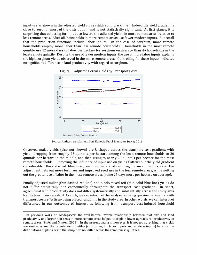
To illustrate the relationship between adjusted yields and transport costs, we plot nonparametric regressions of adjusted yields for sorghum, millet, maize and black/mixed teff in Figure 5.11

The lines represents average yields adjusted for weather and pest shocks (rain more/less than normal, rain earlier/later than usual, frost more/less than normal, and pests more/less than normal) and for input use (labor, chemical fertilizer, pesticides and improved seeds) at each level of transport cost. It is worth noting that variation in weather and pest shocks in the sample was not substantial, and therefore explains little variation in cereal yields over the study area.

Turning to each of the cereals under consideration, observed sorghum yields (not shown) which are actually higher in more remote areas than in less remote areas flatten out once we control for

10 We consider some variables such as plot characteristics to be fixed and not subject to choices made by the farming household. As such, these variables are not netted out (i.e. they are added back into the residual) of the adjusted yield. Note further that altitude is also a fixed characteristic and was included in the initial estimations. However, because it was not statistically significant for any of the cereals, it was dropped from the models. 11 Note that the yields in the survey area are roughly similar to those found in other studies of the Ethiopian highlands (see for example, Yu et al., 2011)

9

input use as shown in the adjusted yield curve (thick solid black line). Indeed the yield gradient is close to zero for most of the distribution, and is not statistically significant. At first glance, it is surprising that adjusting for input use lowers the adjusted yields in more remote areas relative to less remote areas. After all, households in more remote areas use fewer modern inputs. But recall that the production functions include labor inputs. In the case of sorghum, more remote households employ more labor than less remote households. Households in the most remote quintile use 12 more days of labor per hectare for sorghum on average than do households in the least remote quintile. Despite the use of fewer modern inputs, the use of more labor inputs explains the high sorghum yields observed in the more remote areas. Controlling for these inputs indicates no significant difference in land productivity with regard to sorghum.

Figure 5. Adjusted Cereal Yields by Transport Costs

Source: Authors’ calculations from Ethiopia Rural Transport Survey 2011 Observed maize yields (also not shown) are U-shaped across the transport cost gradient, with yields dropping from roughly 23 quintals per hectare among the least remote households to 20 quintals per hectare in the middle, and then rising to nearly 25 quintals per hectare for the most remote households. Removing the influence of input use on yields flattens out the yield gradient considerably (thick dashed blue line), resulting in statistical insignificance. In this case, the adjustment nets out more fertilizer and improved seed use in the less remote areas, while netting out the greater use of labor in the most remote areas (some 25 days more per hectare on average). Finally adjusted millet (thin dashed red line) and black/mixed teff (thin solid blue line) yields do not differ statistically nor economically throughout the transport cost gradient. In short, agricultural land productivity does not differ systematically and substantially across the study area for the four main cereals.12

12 In previous work on Madagascar, the well-known inverse relationship between plot size and land productivity and larger plot sizes in more remote areas helped to explain lower agricultural productivity in remote areas (Stifel and Minten, 2008). In the present analysis, however, it is not too surprising that yields are similar across the remoteness quintiles (controlling for labor inputs and modern inputs) because the distributions of plot sizes in the sample do not differ across the remoteness quintiles.

As such, we can interpret the analysis as being quasi-experimental with transport costs effectively being placed randomly in the study area. In other words, we can interpret differences in our outcomes of interest as following from transport cost-induced household

05

1015

20Q

uint

als

/ ha

0 20 40 60 80Birr/Quintal

Sorghum MilletMaize Teff

Data source: Ethiopia Transport Survey 2011

10

behavioral differences, not from differing geographic characteristics of the study area. One caveat as we have seen, however, is that land holdings do differ, with smaller holdings on average in the more remote areas. The origin of this difference is not entirely clear and does not appear to follow from migration as roughly 4 percent of households in each of the remoteness quintiles are migrants. Nonetheless, as we proceed with the analysis we take care to assess the degree to which our results may depend on land holdings. III. Methodology Having established the quasi-experimental nature of the data, we now describe how we measure the welfare gains from a hypothetical road project that results in a non-marginal reduction in transportation costs between the market town and its surrounding communities. 13

We assume that the market town is small relative to the national market and as such prices are determined outside of the market town. As Jacoby and Minten (2009) note, this implies that the methods described here are thus appropriate for the study of welfare gains from feeder road projects, not trunk road projects that may result in changes in regional/national equilibrium prices.

Let us begin with the setup and then turn to a thought experiment that will help us to conceptualize the benefits of the hypothetical road project. Consider a population of agricultural households that face costs of τ Birr per kilogram to transport freight from their farms to the main market town, Atsedemariam. For simplicity, we label each household by its transportation costs (τ), recognizing that there are numerous households that face the same transportation costs. Households own land (Aτ) and are endowed with labor (Lτ), the distributions in locations τ of which are assumed without loss of generality to be identically distributed. Assume that labor and rental markets exist, where wτ and rτ are the local market clearing wage and rental rates, respectively. Further, assume that hired labor and family labor are perfect substitutes. For simplicity, we suppress the τ label where appropriate. Households produce a vector of crops, y = {y1,…,yk}, using labor (l), land (a) and market-purchased inputs (q), according to concave production functions. Given that prices for the crops in Atsedemariam are 𝑝𝑦 = {𝑝1

𝑦,…, 𝑝𝑘𝑦}, the effective price that sellers face are 𝑝𝑦–τ = {𝑝1

𝑦–τ,…, 𝑝𝑘𝑦–τ }.

Similarly, the effective prices for market-purchased inputs are 𝑝𝑞+τ. Given these assumptions, the income of household τ, 𝑚(𝜏) = (𝑝𝑦 − 𝜏)𝑦 − (𝑝𝑞 + 𝜏)𝑞 − 𝑤𝜏(𝑙 − 𝐿) − 𝑟𝜏(𝑎 − 𝐴), (3) is derived from the value of agricultural production less market-purchased inputs and wage and rental payments. Note that if the household has labor earnings, not all of the household labor endowment is employed on the family farm (i.e. l < L) and labor earnings augment household income. Similarly, rental payments for households that rent out land augment household income because not all household land is used for household production (i.e. a<A). We assume that households have convex preferences over three types of goods: (i) self-produced agricultural goods, x = {x1,…,xk}; (ii) imported bulk goods, c = {c1,…,cn}; and (iii) non-imported bulk and/or imported non-bulk goods, z (prices of which are normalized to one). Goods of type (i) and (iii) are defined in such a way that they do not involve transportation costs, whereas type (ii) goods are imported from Atsedemariam and consequently face effective prices of 𝑝𝑐+τ. Given the 13 This section is based largely on Jacoby and Minten (2009).

11

separability assumption,14

households first choose inputs to maximize income, and then choose their consumption bundles to maximize utility conditional on income. This process yields an indirect utility that varies inter alia with transportation costs, 𝑉�𝑝𝑦 − 𝜏,𝑝𝑐 − 𝜏,𝑚(𝜏)�.

To help conceptualize how we can measure the benefits of a non-marginal decrease in transport costs, consider compensating a remote household with just enough money to make the household members indifferent between being remote (i.e. τ = τ0) and the situation prevailing in the market town (i.e. τ = 0). This sum of money, which we will refer to as 𝜇𝜏 ,15

is the benefit, which represents the willingness-to-pay on the part of the household for the reduction of transportation costs from τ0 to zero. As Jacoby and Minten (2009) point out, 𝜇𝜏 is the equivalent variation of a reduction in transportation costs from τ0 to zero that is implicitly defined by…

𝑉(𝑝𝑦 − 𝜏,𝑝𝑐 + 𝜏,𝑚(𝜏) + 𝜇𝜏) = 𝑉�𝑝𝑦, 𝑝𝑐,𝑚(0)�. (4) The question then is how to estimate 𝜇𝜏 without having to assume a functional form for the utility function (and hence for V(.)). The place to start is by differentiating the identity that defines 𝜇𝜏 in order to determine how the compensation (𝜇𝜏) varies with marginal changes in transportation costs (τ). Relying on the envelope theorem and Roy’s identity, we find that this is… 𝜕𝜇𝜏

𝜕𝜏= ∑ 𝑐𝑗𝑗 + ∑ (𝑦𝑖 − 𝑥𝑖)𝑖 + 𝑞 + 𝜕𝑤𝜏

𝜕𝜏(𝑙 − 𝐿) + 𝜕𝑟𝜏

𝜕𝜏(𝑎 − 𝐴) . (5)

Demand for Wage Rent Transport tonnage effect effect The change in 𝜇𝜏 for a marginal change in transportation costs can be broken down into three components. The first one we shall call the demand for transport tonnage, D(τ), with τ serving as the price16

…

D(τ) = ∑ 𝑐𝑗𝑗 + ∑ (𝑦𝑖 − 𝑥𝑖)𝑖 + 𝑞. (6) Note that this is measured in kilograms and consists of demand for imported bulk goods (c), marketed agricultural surplus (y-x), and demand for agricultural inputs (q). The way to interpret this is that for a one Birr per kilogram increase in transportation costs, households must be compensated by the amount D(τ) to leave them indifferent between the previous situation and the marginally higher τ situation (ignoring the other two components of 𝜕𝜇𝜏

𝜕𝜏 for now).

The second and third components represent how changes in wages and rental rates due to marginal changes in transportation costs affect household incomes, given household endowments of labor and land, and given household optimal choices of labor and land inputs.17

14 This follows from our assumption that household and hired labor are perfect substitutes.

15 Technically, 𝜇𝜏 also depends on the household’s labor and land endowments and should be expressed as 𝜇𝜏(𝐿,𝐴). However, we maintain the simplified notation for ease of reading. 16 We can do this by relying on the composite commodity theorem because market prices are determined outside of the study area and any changes in the effective prices for each of the components are due to changes in transport costs alone. Hence we can think of τ as the common price for all of the commodities. 17 Of course, these changes in income could affect the optimal levels of consumption of own production (x) and of imported bulk goods (c) that appear in the demand for transport tonnage, DT(τ). We follow Jacoby and Minten (2009) here and assume zero income effects in consumption. The implications of this are discussed in footnote 18.

12

Equation (5), however, only gets us partially to our intended benefit measure (𝜇𝜏), as it only represents a change in 𝜇𝜏 due to a marginal change in transportation costs. To measure the benefits of a non-marginal reduction in transportation costs from τ0 to zero, we merely need to integrate both sides of equation (3) (i.e. sum up the marginal benefits for each marginal change in τ)… 𝜇𝜏0 = ∫ [𝐷(𝜏) + 𝑤𝜏(𝑙 − 𝐿) + 𝑟𝜏(𝑎 − 𝐴)]𝑑𝜏𝜏0

0 . (7) As our interest is in the average benefit across all households, not for particular households characterized by labor and land endowments (L, A), we take expectations of both sides. In doing so, we first note that in the local land and labor markets, prices (r and w) adjust such that the average quantity supplied is equal to the average quantity demanded. Thus the average household in each location neither rents in nor rents out land (𝑎(𝑤, 𝑟, 𝜏) = �̅�𝜏), and neither hires in nor hires out labor (𝑙(𝑤, 𝑟, 𝜏) = 𝐿�𝜏). Thus the wage and rental effects drop out of the expectation, leaving… 𝐸�𝜇𝜏0� = ∫ 𝐷(𝜏)𝑑𝜏𝜏0

0 . (8) The benefit measure is thus simply the area under the demand for transport tonnage curve18

from the tonnage demanded at τ = τ0 to τ = 0. This is illustrated in Figure 6.

Figure 6. Measuring Willingness to Pay to Eliminate Transport Costs Transport Cost (Birr/kg) D(τ) = Demand for transport tonnage Consumer surplus lost due τ0 to τ0 > 0 0 D(τ0) D(0) kg

18 Note that assuming that the income effects on consumption are zero means that the demand for transport tonnage curve is effectively a Marshallian demand curve. In other words, we use an uncompensated demand curve to calculate consumer surplus instead of a compensated (Hicksian) demand curve. Jacoby and Minten (2009) point out that if this assumption holds, then the Marshallian consumer surplus �𝐸�𝜇𝜏0��, equivalent variation (EV) and compensating variation (CV) are identical. If the zero income effect assumption does not hold, however, then CV ≤ 𝐸�𝜇𝜏0� ≤ EV.

13

In practice, to estimate the desired integral in equation (8) (i.e. the area under the demand curve), we begin by estimating the conditional expectation function 𝐸[𝐷(𝜏)| 𝜏] = 𝐷�𝜏 nonparametrically at a set of K gridpoints (τ1,…, τK) along the interval [0, τ0]. The expectation is then computed as the sum of these conditional expectation functions weighted by the difference in transport costs within the grid… ∫ 𝐷(𝜏)𝑑𝜏𝜏0

0 = ∑ 𝐷�𝜏𝑘 ∙ �𝜏𝑘 − 𝜏𝑘−1�𝐾

𝑘=2 (9) We calculate this for 10 gridpoints distributed evenly over the transport cost gradient. In this case, the transport cost measure that we use is the cost of transporting a kilogram of tonnage by donkey. We choose to use this measure as it better represents the marginal cost of transporting an additional kilogram compared to our measure of transport costs that includes the imputed value of travel time. This follows because the opportunity cost of time is unlikely to differ substantially for an additional kilogram transported. By ignoring the opportunity cost of time, we recognize that the benefits are likely to be underestimated as the �𝜏𝑘 − 𝜏𝑘−1� component will be too small. Nonetheless, we prefer a conservative estimate rather than an overstated estimate which would occur if we include our measure of time value. A point is worth highlighting is that the model here assumes that in reducing transaction costs, a remote household will adopt the composition of crops produced by a household in the lesser remote areas.19

This implies some substitution out of sorghum and into millet and maize in the least remote quintile compared to all other remoteness quintile. This assumption does not appear to matter too much, however, as it is not obvious that weight of production will differ considerably given the similar yields for these crops and given the similarity in the current total tonnage of agricultural production adjusted for inputs across the transport cost gradient (Figure 7).

Figure 7. Adjusted Total Quantity of Household Agricultural Production

Source: Authors’ calculations from Ethiopia Rural Transport Survey 2011 19 The choice of cropping patterns may indeed change with reductions in transport costs (von Thünen, 1966). Omamo (1998), for instance, shows that cropping patterns in which households devote large shares of land and other resources to low-yielding food crops rather than high-yielding cash crops may indeed be an efficient response to high transport costs to product markets.

050

010

0015

0020

00Ki

logr

ams

0 20 40 60 80Transport Costs (Birr/Quintal)

Total CerealsOil seeds Vegetables

14

There are two reasons, however, to be cautious about the approach described above and why it may overestimate the benefits of rural feeder roads. First, because households often back load consumer goods following trips to the market to sell their agricultural surplus, we may be double counting demand for transport tonnage. For example, if a household transports 100 kilograms of sorghum to the market from the farm, it will likely transport up to 100 kilograms of consumption goods back to the homestead on the return trip rather than to return with an unloaded donkey. There are two ways to handle this issue. We could (a) calculate the transport costs on a one-way basis rather than the current round-trip approach, or (b) exclude consumption items from the calculation of total demand for transport tonnage. In our sensitivity analysis below, we opt for the latter because pre-survey interviews with farmers indicated that trips to purchase/acquire fertilizer and modern seeds did not involve transporting products to the market on the first leg of the trip. If we only calculate the one-way transport costs for input purchases, we will unnecessarily underestimate the costs of acquiring purchased inputs.20

As such, we take a conservative approach and over-correct for potential back loading by reporting benefit estimates that completely exclude bulky consumption goods imported from the market.

The second reason for caution is that while rural road construction will reduce transport costs for remote households, it will not eliminate them entirely. In other words, the compensation necessary to make remote households just indifferent between their situations given current transport costs and the situation prevailing at the market, is an overestimate of the benefit of a hypothetical road. Households may be willing to pay this amount to eliminate transport costs entirely, but no road is capable of doing so. To address this, we err on the side of caution and in addition to considering a project that eliminates transport costs, we also consider one that reduces transport costs by half. This is akin to assuming that motorized transport services will not be provided on the new road. Indeed there is increasing evidence that just because a road is built does not mean that motorized transport services will materialize (Raballand et al., 2011). While it is not clear that this is an issue in our study area,21 we allow for this and recognize that a 50 percent reduction in transport costs is larger that would be expected if only IMT are available. For example, a donkey drawn cart that more than doubles the quantity transported in a shorter period of time would result in transport costs per quintal falling by more than 50 percent. As such, even considering IMT instead of trucks, reducing transport costs by half provides a conservative estimate of the benefits.22

Consequently, we proceed with the two equally strong assumptions of transport cost reductions to estimate upper (cost elimination) and lower (50 percent cost reduction) bounds of the benefits.

20 In addition to making trips to the market town to acquire the inputs, roughly two thirds of the sample households made more than one trip to the market town in order to arrange the purchase of the inputs. In ignoring these additional trips, we acknowledge that we underestimate the demand for transportation. 21 There appears to currently be ample supply of transport services. Based on the marketed agricultural surplus estimated for the study area, an average of four trucks per week transport agricultural products from Atsedemariam to markets beyond. This is also consistent with informal interviews conducted with traders in Atsedemariam prior to the survey, and with truckers after the survey. 22 Note further that a 50 percent reduction in the 2 Birr per kilometer per quintal transport cost for the most remote households in our sample results in a cost that is considerably more than the 0.14 Birr per kilometer per quintal transport costs observed on average for similar sized trucks on trunk roads between the wholesale markets (based on a survey of the 31 major wholesale markets in Ethiopia conducted by the authors). While we do not expect the transport costs on a rural feeder road to drop all the way to the trunk road costs, we equally do not expect them to be seven-fold larger than these costs.

15

To illustrate how reducing costs by half applies to the approach described above, consider an equivalent variation (𝜇𝜏) of a reduction in transportation costs from τ to 𝜏

2 that is implicitly defined

by… 𝑉(𝑝𝑦 − 𝜏,𝑝𝑐 + 𝜏,𝑚(𝜏) + 𝜇𝜏) = 𝑉 �𝑝𝑦 − 𝜏

2,𝑝𝑐 + 𝜏

2,𝑚�𝜏

2�� (4’)

This analogously leads to the following average benefit for households located at 𝜏… 𝐸(𝜇𝜏) = ∫ 𝐷(𝜏)𝑑𝜏𝜏

𝜏 2⁄ (8’) which is the area under the demand for transport tonnage curve from τ to 𝜏

2. This can be estimated

using equation (9) by calculating the benefits of eliminating transport costs for the most remote households (in bracket 10) and subtracting from it the benefits of eliminating transport costs for the households whose transport costs are half of those of the most remote households (in bracket 5)… ∫ 𝐷(𝜏)𝑑𝜏𝜏

𝜏 2⁄ = ∑ 𝐷�𝜏𝑘 ∙ �𝜏𝑘 − 𝜏𝑘−1�𝐾

𝑘=2 − ∑ 𝐷�𝜏𝑘 ∙ �𝜏𝑘 − 𝜏𝑘−1�𝐾 2⁄

𝑘=2 (9’) In the analysis that follows, we present the complete benefit estimates as described in equation (9), as well as those described in equation (9’) both with and without imported consumption goods. A final consideration is whether to incorporate nonfarm earnings in the estimate of benefits. Given evidence from other countries that greater non-agricultural labor activities are found nearer to towns (Fafchamps and Shilpi, 2005; Stifel and Minten, 2008; Jacoby and Minten, 2009), we might also wonder if the benefit estimate in equation (9) underestimates the true benefits. This appears not to be the case for several reason. First, only 12 percent of households in the sample have non-farm earnings from either non-farm labor or from household non-farm enterprises (see Table 4). Of these households, more are actually found in the more remote communities. It is therefore not clear that there are greater non-agricultural activities nearer to the market town. Second, median annual non-farm earnings do not differ substantially across the transport cost gradient. Third, those households that have non-farm earnings have roughly 20 percent lower levels of household consumption expenditures compared to households without non-farm earnings. This suggests that there might be push factors that result in households engaging in nonfarm activities, rather than being drawn into such activities by potential earnings premia due to lower transport costs. 23

Nonetheless, we test whether our benefit estimates are affected by differential non-farm earnings by augmenting equation (8) with the difference between the mean non-farm earnings for the most remote bracket and for the least remote bracket (Jacoby and Minten, 2009). Although not shown here, we find that the mean earnings differences are marginal and our benefits estimates are

23 In certain instances there are incentives that push households with weak non-labor asset endowments and who live in risky agricultural zones into allocating household labor to nonfarm activities. Although households frequently do turn to the nonfarm sector as an ex ante risk reduction strategy, distress diversification into low-return nonfarm activities is also observed as an ex post reaction to low farm income (Von Braun, 1989; Haggblade, 2007). This differs from such factors as earnings premia from high productivity/high income activities may attract, or pull, some household labor into nonfarm employment (Dercon and Krishnan, 1996; Barrett et al., 2001; Lanjouw and Feder, 2001; Reardon et al., 2001; Haggblade, 2007). These high-return nonfarm jobs may serve as a genuine source of upward mobility (Lanjouw, 2001).

16

unaffected. This is not surprising considering the similarity of non-farm earnings across the transport cost gradient. We therefore do not adjust our benefit measures to account for nonfarm earnings. Table 4. Non-Farm Earnings by Transport Costs

Pct. of HH with

Median NF Percent difference in HH Expenditures

NF earnings earnings* (Birr) between those w/ and w/o NF earnings Least Remote 7

1,000 20.0

Quintile 2 12

1,300 26.1 Quintile 3 13

1,200 22.8

Quintile 4 14

1,180 22.2 Most Remote 17

1,102 18.4

Total 12 1,102 22.1 * Among those with non-farm earnings Source: Authors’ calculations from Ethiopia Rural Transport Survey 2011 IV. Willingness to pay for transport cost reduction Figure 8 shows the nonparametric estimates of the demand for transport tonnage curve (D(τ)) along with its components – marketed agricultural surplus, imported consumption goods and purchased agricultural inputs. As expected, the transport cost gradients for each of the components is negative. Overall demand for freight drops by almost 50% from over 1,100 kg among the least remote households to just over 500 kg for those in the more remote areas. Each of the components contributes roughly equally to the total decline in total demand. Consistent with the stylized facts presented in Section II, purchases of inputs drop to very low levels in the more remote areas, compared to demand for nearly 250 kg on average in the least remote areas.

Figure 8. Demand for Transport Tonnage and Transport Costs

Source: Authors’ calculations from Ethiopia Rural Transport Survey 2011

025

050

075

010

0012

50kg

0 20 40 60 80Transport Cost (Birr/Quintal)

Total Freight Imported ConsumptionAgricultural Surplus Input Purchases

17

Marketed agricultural surplus makes up the largest component of total demand for transport tonnage, followed by imported consumption. We note that because the total demand for tonnage from imported consumption is less than from marketed agricultural surplus, subtracting demand due to imported consumption to avoid double counting from back loading will likely lead to an underestimate of demand for total tonnage. As such, the calculations of benefits without imported consumption should be interpreted as conservative estimates. Using equation (9) and the estimates of total demand for transport tonnage (D(τ)) illustrated in Figure 8, we estimate the benefits of a hypothetical rural feeder road project that reduces the transport costs to zero. This is equivalent to reducing transport costs for the most remote – from our 10 gridpoints analysis - households by 5 US Dollars per quintal (50 US Dollars per metric ton). The resulting benefit is 3,590 Birr of annual income for the most remote households and 2,338 Birr on average for all households in the sample (see Table 5). Although this does not appear in the table, we calculate that 35 percent of this benefit is due to lower effective costs of imported consumption goods, and 48 percent is due to higher effective prices for marketed agricultural surplus. To put the total benefits in perspective, they represent 54 percent of the value of household consumption for the most remote households, and 15 percent for all households. Table 5. Benefit Estimates for Transport Cost Reduction

Reducing transport costs to zero for…

Reducing transport costs by half for…

Most remote HH Average HH Most remote HH Average HH Birr / Year

Total

Unadjusted 3,590 2,338

1,624 1,314

Adjusted* 3,522 2,271

1,650 1,291

Without Consumption

Unadjusted 2,320 1,555

980 846

Adjusted* 2,270 1,499

1,013 829

Percent of Household Consumption

Total

Unadjusted 54.0 15.3

24.4 8.6

Adjusted* 53.0 14.9

24.8 8.4

Without Consumption

Unadjusted 34.9 10.2

14.7 5.5

Adjusted* 34.2 9.8

15.2 5.4

* Adjusted for landholdings Source: Authors’ calculations from Ethiopia Rural Transport Survey 2011 Sensitivity Analysis As noted previously, there are several reasons why these benefit estimates may be overstated. First, we may be double counting the benefits as a result of back loading. Adjusting for this by excluding imported consumption in our calculations results in benefit estimates that are roughly 35 percent less (i.e. 2,320 Birr for the most remotes households and 1,555 Birr for the average household). In this case, the benefits represent 35 percent of consumption for the most remote households and 10 percent of consumption for the average household.

18

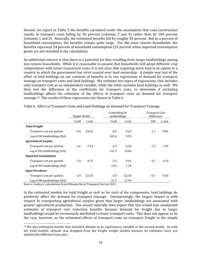
Second, we report in Table 5 the benefits calculated under the assumption that road construction results in transport costs falling by 50 percent (columns 3 and 4) rather than by 100 percent (columns 1 and 2). Naturally, the estimated benefits fall by roughly 50 percent. But as a percent of household consumption, the benefits remain quite large. For the most remote households, the benefits represent 24 percent of household consumption (15 percent when imported consumption goods are not included in the calculation). An additional concern is that there is a potential for bias resulting from larger landholdings among less remote households. While it is reasonable to assume that households will adopt different crop compositions with lower transaction costs, it is not clear that acquiring more land is an option in a country in which the government has strict control over land ownership. A simple way test of the effect of land holdings on our estimate of benefits is to run regressions of demand for transport tonnage on transport costs and land holdings. We estimate two types of regressions. One includes only transport cost as an independent variable, while the other includes land holdings as well. We then test the difference in the coefficients for transport costs, to determine if excluding landholdings affects the estimates of the effects of transport costs on demand for transport tonnage.24

The results of these regressions are shown in Table 6.

Table 6. Effect of Transport Costs and Land Holdings on Demand for Transport Tonnage

Simple Model

Controlling for landholdings

Transport Cost Difference

Coeff t-stat Coeff t-stat Diff z-stat

Total Freight

Transport cost per quintal -9.5 -10.66

-8.4 -9.42

-1.1 -0.85

Log of HH landholdings (HA)

183.4 9.95

Agricultural Surplus

Transport cost per quintal -4.6 -7.43

-3.3 -5.20

-1.3 -1.49

Log of HH landholdings (HA)

141.3 10.66

Imported Consumption

Transport cost per quintal -2.4 -4.75

-2.5 -4.41

0.1 0.10

Log of HH landholdings (HA)

13.6 1.18

Input Purchases

Transport cost per quintal -2.9 -22.50

-2.8 -22.58

-0.1 -0.60

Log of HH landholdings (HA) 31.7 11.99

Source: Authors’ calculations from Ethiopia Rural Transport Survey 2011 In the estimated models for total freight as well as for each of the components, land holdings do positively affect the demand for transport tonnage. Unsurprisingly, the largest impact is with respect to transporting agricultural surplus given that larger landholdings are associated with greater agricultural production. One would naturally then expect that this would bias unadjusted estimates of transport cost reduction benefits because demand for freight due to larger landholdings would be erroneously attributed to lower transport costs. This does not appear to be the case, however, as the estimated effects of transport costs on transport freight in the simple 24 We also estimated models that included altitude as an explanatory variable in the second model. As with the yield models, altitude was dropped from the freight weight models because its estimates were not statistically different from zero.

19

model do not differ statistically from the estimated effects in the models in which landholdings are also included. Although the results in Table 6 suggest that there is no impact of landholding on the demand-for-freight – transport-cost gradient, we also adjust our estimates of the benefits of reduced transport costs for landholdings. Using the approach of equation (3), we net out the effect of landholdings on demand for transport tonnage, and then proceed to estimate the benefits using equation (9). These estimates, labeled “adjusted” in Table 5, do not differ substantially from the unadjusted estimates. Consequently, the remainder of the analysis focuses on the unadjusted estimates of benefits. V. Cost-Benefit Analysis Cost-benefit calculations help to further put these benefit estimates in perspective. In particular, we calculate internal rates of return (IRR) for road projects in the survey area in which we consider different lengths for the road. The idea is that a road spanning the entire length of the sample area may not be optimal, and that a shorter road may be preferable. On the cost side, according to the Ethiopian Roads Authority, it costs roughly 800,000 Birr to construct one kilometer of gravel road in the survey area.25 But again, we err on the conservative side and assume a cost of 1 million Birr per kilometer. With some 35 kilometers separating the most remote households from the market in Atsedemariam, a gravel road spanning the length of the survey area will cost roughly 35 million Birr (2.1 million US Dollars). We assume that with annual maintenance costs roughly equal to 5 percent of construction costs, a road of this type can last at least 10 years (Donnges et al, 2007).26

On the benefits side, we estimate the total benefit by multiplying the average benefit in the sample27

25 This is consistent with previous costs in Ethiopia. For example, in 2008/9, it cost 260,000 Birr on average to construct a kilometer of rural gravel roads (Ethiopian Roads Authority, 2009). This figure comes from the second year of the third phase of the Ethiopian Rural Sector Development Programme (RSDP), in which 445.7 million Birr was distributed for the construction of rural roads and bridges, from which 1,710 km of rural roads were built. Given inflation, this is conservatively equivalent to 730,000 Birr per kilometer at the end of 2011.

by 5,180 households in the study area. For a road that spans the entire 35 kilometers of the sample area, the benefits are calculated as described in section III, with compensation estimated in each bracket such that transport costs are either eliminated or cut in half. For shorter distance roads, however, the calculation is broken down into two components. For example, for a 28 kilometer road, the standard benefit measurement approach applies to all households within 28 kilometers of the market town (i.e. the first 8 brackets). That is, for these households we estimate the compensation needed to make them indifferent between the prices they currently face and those they would face in the market town. For those households that are more than 28 kilometers from the market town, the approach is slightly different because while the road does not reach them directly, it will reduce their transportation costs. To illustrate, consider households that are 35 kilometers from the market town. A 28 kilometer road that eliminates transport costs entirely leaves the most remote households in a position where they face transport costs that are equivalent to those faced by households that are currently 7 kilometers (35 – 28 kilometers) from the market town. Thus the benefit of the road to these households is the compensation necessary to make

26 In our IRR calculations, we do not account for negative externalities such as road accidents and environmental effects, nor positive benefits such as improved access to health facilities and schools. 27 Because households in the sample are not evenly distributed across the transport cost/distance gradient (see Figure 2), the average benefit is calculated as a weighted average where the weights are the probability of the household being in the particular transport cost bracket.

20

them just indifferent between the prices they currently face and the prices they would face if they were 7 kilometers from the market. Thus the average benefit for these households is… 𝐸�𝜇𝜏35� = ∫ 𝐷(𝜏)𝑑𝜏𝜏35

𝜏7 (8’’)

Table 7 presents the results of the benefit and cost estimates for various lengths of roads, with ratios of initial construction costs to the one-year benefits shown in columns 2 and 3. These ratios range from a low of 1.5 for a 7 kilometer road that reduces transport costs to zero and when consumption is included in the benefit estimate, to a high of 6.4 for a 35 kilometer road that reduces transport costs by half for everyone and when imported consumption is excluded from the benefit estimate. For a 35 kilometer road, the ratio ranges from 2.3 to 6.4. This 2.3 difference between costs (higher) and the benefits (lower) can be interpreted as taking 2.3 years for the accrued benefits to outweigh the costs (ignoring discounting, annual maintenance costs, and population and income/productivity growth that might take place over this time period). In all of the scenarios in the table, the initial cost-benefit ratios are roughly similar up to halfway through the study area. They then rise quicker for 28 and 35 kilometer roads, indicating that the returns to constructing a road drop off over this interval. To account for discounting and annual maintenance costs, we calculate IRR for each road length under the different assumptions about transport cost reduction and demand for transport tonnage. We present IRR estimates of benefits that include and exclude demand for imported consumption, and for estimates for both the elimination (upper bound) and a 50 percent reduction (lower bound) of transport costs. With regard to the former, we prefer to focus on the estimates that exclude imported consumption as this corrects for the observed pattern of back loading. For the latter, we interpret the 50 percent reduction in costs as a conservative estimate of the returns to a road on which only IMT such as donkey-drawn carts are made available, while the elimination of costs is more akin to the provision of motorized transportation. As such, we are cognizant that the true benefits are likely to be somewhere in between the two bounds.

Table 7. Estimated Internal Rates of Return for Different Road Lengths Length of gravel Initial Cost/Benefit*

Internal Rate of Return**

road (km)… Total W/o Cons Total W/o Cons Road reduces travel cost to zero

7

1.5 2.4

0.60 0.35 14

1.6 2.4

0.58 0.34

21

1.6 2.4

0.57 0.34 28

1.9 2.8

0.47 0.28

35

2.3 3.5

0.37 0.20 Road reduces travel cost by half

7

2.9 4.6

0.27 0.15 14

3.1 4.8

0.25 0.14

21

3.2 5.0

0.23 0.12 28

3.4 5.3

0.20 0.11

35 4.1 6.4 0.14 0.07 * Assuming a cost of Birr 1 million per kilometer ** Assuming a 10-year life span of the road and 5 percent annual maintenance costs Source: Authors’ calculations from Ethiopia Rural Transport Survey 2011

21

In the last two columns of Table 7, we find that the IRRs vary from 60 percent for a 7 kilometer road to 7 percent for a 35 kilometer road. If we take a conservative approach to tonnage demand (i.e. exclude consumption in the calculation), then the benefits range from 35 percent to 7 percent. We note that as with the cost-benefit ratios, there is an evident drop in the IRR for the longer roads. For example, when we calculate benefits without consumption goods and assuming an elimination of transport costs (top section of last column), the IRRs consistently range from 12 to 34 percent for roads whose lengths are between 7 and 21 kilometers. The IRR falls to a range of 11 to 28 percent for a 28 kilometer road, and further to 7 to 20 percent for a 35 kilometer road. Although this does indicate that the returns fall for a road spanning the more distant part of the survey area, it is worth noting that a 35 kilometer road is likely to also benefit households beyond the study area. Because these households are not included in the sample, the benefits accruing to them are not included in the estimate of total benefits. As such, the benefits are likely underestimated, as are the IRR. These IRR compare favorably with those estimated by the World Bank (2003) for rehabilitation projects on major trunk roads in Ethiopia that range from 12 percent to 48 percent.28 Although the benefits for the major trunk roads are calculated in a different manner (e.g. based on the reduction of user costs on existing roads),29 these results suggest that investments in rural feeder roads are cost-effective ways to help reduce widespread poverty even in an unfavorable setting such as our study area. For example, despite recent evidence from West Africa suggesting that roads should be targeted to areas with more opportunity for non-farm activities and away from areas with low agricultural surplus because the returns for the latter are too low (Gachassin et al., 2010), 30

we find that in Ethiopia this is not necessarily the case. Even in circumstances where the provision of motorized transport services is not guaranteed and transport services are instead limited to rudimentary IMT, we estimate that the returns to rural feeder roads are relatively high and that they are rightly placed as an integrated component of rural infrastructure development.

28 For example, the estimated IRRs are between 37.5 and 47.8 percent for the Nazareth-Assela road, 12.2 and 18.5 percent for the Woreta-Gob Gob road, 35.2 and 48.5 percent for the Adigrat-Adwa road, 22.3 and 31.3 percent for the Nekemte-Mekenajo road, and 13.3 and 20.9 percent for the Dera-Magna road (World Bank, 2003). 29 Recall that the approach to estimating benefits in this paper cannot be applied to trunk roads because of the assumption of a small market and exogenously determined prices. Rehabilitation of major trunk roads that reduce transaction costs has been found to affect equilibrium prices (Minten et al., 2012). 30 Jacoby and Minten (2009) also find that the bulk of the benefits estimated in their Madagascar sample derive from non-farm earnings.

22

VI. Conclusions This paper assesses the benefits of rural feeder roads in Ethiopia. As part of an effort to revitalize the agricultural and rural sector since liberalization, the government of Ethiopia has emphasized the development of the rural infrastructure. Indeed, rural infrastructure development and maintenance are seen as central to the growth agenda in the Sustainable Development and Poverty Reduction Program (SDPRP, 2002) and its successor, the Plan for Accelerated and Sustained Development to End Poverty (PASDEP, 2006). It is thus important to understand the magnitude of the benefits of these investments. There are two significant issues, however, that complicate quantifying the economic benefits of improved rural transport infrastructure. These are (a) the conceptualization of benefits and ultimately the measure that is used, and (b) establishing the direction of causality (do roads lead to more prosperous areas, or are roads built to more prosperous areas?). The benefit measure in this analysis is based on household demand for transport tonnage in which we estimate households’ willingness-to-pay for reduced transport costs (i.e. the area under the demand for transport curve) using an approach developed by Jacoby and Minten (2009). This approach complements recent analyses that find significant consumption/income benefits of access to all-weather roads for households in the Ethiopian Rural Household Survey (Dercon et al., 2009, Wondemu and Weiss, 2010), and that find a growth-spurring impact of asphalt roads but not gravel roads using time series data (Worku, 2010). Our approach, however, also allows for a more complete accounting of the surplus gains that stem from the additional economic activity generated by road improvements. We address the problem of causation in a quasi-experimental manner by conducting a household survey of a relatively homogeneous region in northwestern Ethiopia. This sample area was selected purposefully in order that the primary differences between communities in the otherwise homogeneous region are the transport costs between the communities and the particular market to which community members travel. In our study area, these transportation costs differ substantially within the region, but they differ because of the geography of the region, not because of road placement. Jacoby and Minten (2009) argue that when a sample is identified in this manner, “a comparison of household behavior along this steep transport cost gradient approximates the long run adjustments to an exogenous road improvement.” We find that the geographical characteristics in our survey area, as measured by reported land quality and land productivity for sorghum, millet, maize and teff, do not differ systematically and substantially. As such, the analysis can be interpreted as being quasi-experimental with transport costs effectively being placed randomly in the study area. In other words, we can interpret differences in our outcomes of interest as following from transport cost-induced household behavioral differences, not from differing geographic characteristics of the study area. Based on our estimate of benefits, a hypothetical feeder road project in this rural setting that reduces the transport costs for the most remote households by 50 US Dollars per metric ton, would result in benefits worth roughly 35 percent of household consumption for these households. These benefits range from 15 percent to 54 percent depending on our assumptions. A simple cost-benefit analysis reveals that a hypothetical 10-year road constructed halfway through our study area has an IRR ranging from 12 percent to 34 percent. The lower range of estimates is consistent with transport service delivery that is limited to rudimentary IMTs such as donkey-drawn carts. As such, even if trucks fail to ply the new road to collect agricultural products for sale in the market (Raballand, 2010, 2011), the provision of IMTs is sufficient to generate a relatively high rate of

23

return. These returns fare favorably to IRR calculated for trunk road projects, suggesting that the rural feeder roads are rightly placed as an integrated component of rural infrastructure development in Ethiopia. We note that these benefit estimates ignore the potential dynamic gains from opportunities for expansion of the non-farm sector, which are currently limited in the sample area and appear to serve more as a safety net than as sources of genuine upward mobility. Further, they do not incorporate gains due to improved access to such services as health and education for which community members in the study area expressed yearning. Finally, while we caution that the benefits estimated in this paper are particular to the study area, the results are nonetheless informative in shedding light on the nature of the benefits of constructing feeder roads in similar remote rural communities. In particular, they suggest that investments in rural feeder roads may be cost-effective ways to help reduce widespread poverty even in unfavorable settings where (a) small-scale farmers have low levels of marketed agricultural surplus, (b) nonfarm earnings opportunities are currently negligible, and (c) the provision of motorized transport services is not guaranteed.

24

References Binswanger, Hans P., Shahidur R. Khandker, and Mark R. Rosenzweig. 1993. “How Infrastructure

and Financial Institutions Affect Agricultural Output and Investment in India.” Journal of Development Economics, 41:337–66.

Butler, J.S., and Christine Moser. 2010. “Structural Model of Agricultural Markets in Developing Countries.” American Journal of Agricultural Economics, 92(5): 1365-1378.

Barrett, Christopher, Thomas Reardon, and Patrick Webb. 2001. “Nonfarm Income Diversification and Household Livelihood Strategies in Rural Africa: Concepts, Dynamics, and Policy Implications.” Food Policy, 26(4): 315-331.

Dercon, Stefan. 1995. “On Market Integration and Liberalisation: Method and Application to Ethiopia.” Journal of Development Studies, 32(1): 112-143.

Dercon, Stefan, Daniel Gilligan, John Hoddinott, and Tassew Woldehanna. 2009. “The Impact of Agricultural Extension and Roads on Poverty and Consumption Growth in Fifteen Ethiopian Villages.” American Journal of Agricultural Economics, 91(4): 1007-1021.

Dercon, Stefan, and Pramila Krishnan. 1996. “Income Portfolios in Rural Ethiopia and Tanzania: Choices and Constraints.” Journal of Development Studies, 32(6): 850-875.

Donnges, Chris, Geoff Edmonds, and Bjorn Johannessen. 2007. “Rural Road Maintenance - Sustaining the Benefits of Improved Access.” International Labour Organization (ILO), Bangkok, Thailand.

Ethiopian Roads Authority (ERA). 2009. “RSDP Performance: 12 Year Assessment.” ERA, Addis Ababa.

Ethiopian Roads Authority (ERA). 2011. “RSDP 13 Years Performance and Phase IV.” ERA, Addis Ababa.

Fafchamps, Marcel, and Forhad Shilpi. 2005. “Cities and Specialisation: Evidence from South Asia.” Economic Journal, 115(503): 477-504.

Fafchamps. Marcel, and Forhad Shilpi. 2003. "The spatial division of labour in Nepal." Journal of Development Studies, 39(6): 23-66.

Fan, Shenggen, and Peter Hazell. 1999. “Are Returns to Public Investment Lower in Less-Favored Rural Areas? An Empirical Analysis of India.” International Food Policy Research Institute (IFPRI) Environment and Production Technology Division Discussion Paper No. 43. Washington, DC.

Fan, Shenggen, and C. Chan-Kang. 2004. ‘Returns to Investment in Less-Favored Areas in Developing Countries: A Synthesis of Evidence and Implications for Africa’, Food Policy, 29 (4): 431–44.

Gachassin, Marie, Boris Najman, and Gael Raballand. 2010. “The Impact of Roads on Poverty Reduction: A Case Study of Cameroon.” Policy Research Working Paper Series 5209. The World Bank. Washington DC.

Gibson, John, and Scott Rozelle. 2003. “Poverty and Access to Roads in Papua New Guinea.” Economic Development and Cultural Change, 52(1): 159-185.

Gollin, Douglas, and Richard Rogerson. 2010. “Agriculture, Roads, and Economic Development in Uganda.” National Bureau of Economic Research Working Paper 15863

25

Gouesnard, Brigitte, Cécile Rebourg, Claude Welcker and Alain Charcosset. 2002. “Analysis of photoperiod sensitivity within a collection of tropical maize populations.” Genetic Resources and Crop Evolution, 49: 471-481

Haggblade, Steven. 2007. “Alternative Perceptions of the Rural Nonfarm Economy.” In Haggblade, Steven, Peter Hazell and Thomas Reardon, eds. Transforming the Rural Nonfarm Economy. Johns Hopkins University Press: Baltimore.

Jacoby, Hanan. 2000. ‘Access to Markets and the Benefits of Rural Roads’, The Economic Journal, 110: 713–37.

Jacoby, Hanan, and Bart Minten. 2009. “On Measuring the Benefits of Lower Transport Costs.” Journal of Development Economics, 89(1): 28-38.

Khandker, Shahidur, Zaid Bakht, and Gayatri Koolwal. 2009. “The Poverty Impact of Rural Roads: Evidence from Bangladesh.” Economic Development and Cultural Change, 57(4): 685-722.

Lanjouw, Peter. 2001. “Nonfarm Employment and Poverty in Rural El Salvador.” World Development 29(3): 529-547.

Lanjouw, Peter, and Gershon Feder. 2001. “Rural Non-Farm Activities and Rural Development: From Experience Towards Strategy.” World Bank Rural Development Strategy Background Paper No. 4. World Bank: Washington, DC.

Lebo, J., Schelling, D., 2001. “Design and Appraisal of Rural Transport Infrastructure: Ensuring Basic Access for Rural Communities.” World Bank Technical Paper, Vol. 496. The World Bank, Washington, DC.

Lokshin, Michael, and Ruslan Yemtsov. 2005. “Has Rural Infrastructure Rehabilitation in Georgia Helped the Poor?” World Bank Economic Review, 19:311–33.

Minten, Bart, David Stifel, and Seneshaw Tamiru. 2012. “Structural Transformation in Ethiopia: Evidence from Cereal Markets.” Mimeo, International Food Policy Research Institute (IFPRI), Addis Ababa.

Moser, Christine, Christopher Barrett, and Bart Minten. 2009. “Spatial Integration at Multiple Scales: Rice Markets in Madagascar.” Agricultural Economics, 40(3): 281-294.

Mu, Ren, and Dominique van de Walle. 2007. “Rural roads and poor area development in Vietnam.” Policy Research Working Paper, no. 4340. The World Bank, Washington, DC.

Omamo, Steven Were. 1998. “Transport Costs and Smallholder Cropping Choices: An Application to Siaya District, Kenya.” American Journal of Agricultural Economics, 80: 116-123.

Osborne, Theresa. 2005. “Imperfect Competition in Agricultural Markets: Evidence from Ethiopia.” Journal of Development Economics, 76: 405-428.

Raballand, Gael, Patricia Macchi, and Carly Petracco. 2010. “Rural Road Investment Efficiency: Lessons from Burkina Faso.” The World Bank, Washington DC.

Raballand, Gael, Rebecca Thornton, Dean Yang, Jessica Goldberg, Niall Keleher, Annika Muller. 2011. "Are rural road investments alone sufficient to generate transport flows? Lessons from a randomized experiment in rural Malawi and policy implications." Policy Research Working Paper Series 5535, The World Bank.

Reardon, Thomas, Julio Berdegué, and Germán Escobar. 2001. “Rural Nonfarm Employment and Incomes in Latin America: Overview and Policy Implications.” World Development 29(3): 295-409.

26

Ruel, Marie. 2003. “Operationalizing Dietary Diversity: A Review of Measurement Issues and Research Priorities.” The Journal of Nutrition, 133: 3911S-3926S.

Stifel, David, and Bart Minten. 2008. “Isolation and Agricultural Productivity.” Agricultural Economics, 39(1): 1-15.

USDA (United States Department of Agriculture) Human Nutrition Information Service. 1992. “Food Guide Pyramid: A Guide to Daily Food Choices.” Home and Garden Bulletin. No. 249. USDA and Health and Human Resources. Washington, DC.

von Braun, Joachim. 1989. “The Importance of Non-Agricultural Income Sources for the Rural Poor in Africa and Implications for Food and Nutrition Policy.” PEW/Cornell Lecture Series on Food and Nutrition Policy. Cornell Food and Nutrition Policy Program: Ithaca, NY.

von Thünen, Johann Heinrich. 1966. Von Thünen's Isolated State. Translated by C.M. Wartenberg. Edited by Peter Hall. Oxford: Pergamon Press.

World Bank. 2005. “Well-Being and Poverty in Ethiopia: The Role of Agriculture and Agency.” World Bank, Washington D.C..

World Bank. 2007. “Agriculture for Development. World Development Report 2008.” World Bank, Washington D.C.

WHO (World Health Organization). 1996. “Preparation and Use of Food-Based Dietary Guidelines.” WHO Technical Report, Series 880. Report of a Joint FAO/WHO Consultation. WHO, Geneva, Switzerland.

Wondemu, Kifle Asfaw, and John Weiss. 2010. “Rural Roads and Development: Evidence from Ethiopia.” Mimeo: University of Bradford, UK.

Worku, Ibrahim. 2010. “Road Transport in Ethiopia: Trends, Stock of Achievements, and Impact on Overall and Sectoral Economic Growth.” Mimeo: Ethiopian Development Research Institute.

World Bank. 2003. “Ethiopia - Second Road Sector Development Program Project: Project Appraisal.” Washington, DC.

Yu, Bingxin, Alejandro Nin-Pratt, José Funes, and Sinafikeh Gemessa. 2011. “Cereal Production and Technology Adoption in Ethiopia.” International Food Policy Research Institute (IFPRI) Discussion Paper No. 01131. Washington, DC.