Economic and Political Inequality: The Role of Political ... · Economic and Political Inequality:...

Economic and Political Inequality:The Role of Political Mobilization

Francesc Amat†

Pablo Beramendi‡

January 29, 2016

Abstract

This paper analyzes the relationship between economic and political inequality. Beyondthe view that inequality reduces turnout we document a non-linear relationship between them.To explain these patterns we argue that parties’ strategies to target and mobilize low incomevoters reflect the level of economic inequality and development. Under high inequality and lowdevelopment, clientelism becomes the dominant form of political competition and turnout in-equality declines. As societies grow and inequality recedes, clientelism becomes suboptimal andparties turn to mobilize voters around programmatic offerings. As a result, turnout inequalityincreases. Empirically, we produce two analyses. First, we identify the relationship betweenpolitical mobilization strategies, inequality and turnout by exploiting the randomized allocationof anti-fraud measures across Brazilian municipalities in the early 2000s. Second, we addressthe generalizability of our findings by carrying out a cross-national multilevel analysis of therelationship between inequality, strategies for political mobilization, and turnout inequality.

∗Paper prepared for presentation at the National School of Development, Peking University, MondayOctober 26th 2015. Previous versions were presented at the 2015 APSA Meetings, San Francisco September3-6, the Comparative Politics Workshop at the University of Wisconsin, Madison, the Duke PE workshop,and the CP colloquium at Princeton University. Earlier explorations of ideas similar to the ones in this paperwere presented at the Workshop on Economic Inequality and the Quality of Democracy UBC Vancouver;the IPEG Seminar, UPF, Barcelona; and the Comparative Politics Workshop at Washington University,St. Louis. We thank participants in all these events as well as Ana de la O, Atila Abdulkadiroglu, BetulDemirkaya, Tim Feddersen, Hector Galindo, Ruben Enikolopov, Herbert Kitschelt, Philipp Rehm, GuillermoRosas, David Rueda, and Susan Stokes for their comments on previous versions of this manuscript. We thankAsli Cansunar and Haohan Chen for excellent research assistance. Finally, we thank Herbert Kitschelt forsharing his data on types of political competition, and Claudio Ferraz for sharing data that allowed us toperform the experimental analysis of Brazilian municipalities.†Post-doctoral Research Fellow, IPEG, Universitat Pompeu Fabra‡Associate Professor, Department of Political Science, Duke University.

1 Introduction: Puzzles and Outline

The nexus between economic and political inequality lies at the heart of democratic

theory and political economy (Przeworski, 2010). Dahl defined democracy as a set of pro-

cedures guided by the principle of “equal consideration”, that is the notion that “ In cases

of binding collective decision, to be considered as an equal is to have one’s interests taken

equally into consideration by the process of decision-making” (Dahl, 1991, p.87). In other

words, the ability to participate in politics, influence policy, and government’s responsive-

ness are what determines whether citizens truly are ıt political equals under democracy. A

pre-requisite for this conception of democracy to work effectively is that citizens’ positive

freedoms (Berlin, 1958) are not undermined by a reduction in their capability set due to

material deprivation (Sen, 1992). The undermining of positive freedoms may take various

forms, from the capture of the vote choice in exchange for material benefits to the induced

self-exclusion of the electoral body altogether. Who chooses to vote, how, and why, has in

turn major implications for distributive politics and economic outcomes, feeding back into

the linkage between economic and political inequality.

The negative impact of inequality on political engagement and electoral turnout is a

recurrent theme in comparative politics. Inequality and poverty limit access to the necessary

resources individuals need to engage in politics, whether material or informational (Verba

et al., 1995; Solt, 2008; Gallego, 2010; Mahler, 2008); alter the structure of informational

networks under which individuals operate politically (Bond et al., 2012; Abrams, Iversen and

Soskice, 2011); shape the levels of political polarization (Pontusson and Rueda, 2010), or

alter the incentives of political parties to target different types of voters in different electoral

systems (Anduiza Perea, 1999; Anderson and Beramendi, 2012; Gallego, 2014). Jointly,

these findings help understand an important empirical regularity from the standpoint of the

1

linkages between economic and political inequalities: poorer citizens are less likely to vote

than rich ones, and even more so in more unequal societies. The lack of engagement of the

poor reduces the strength of pro-redistributive coalitions at the same time that increasing

inequality feeds back into the political participation of low-income citizens (Franzese and

Hays, 2008).

Yet, younger and less developed democracies call into question the generalizability

of this well established result by previous literature. In less developed and very unequal

democracies poor voters often seem as willing (if not more) to engage in politics than their

counterparts in rich democracies (Krishna, 2008; Stokes et al., 2013). As a matter of fact,

the relationship between inequality and electoral turnout in the developing world reverses

the patterns observed in wealthier democracies: higher levels of inequality are associated

with high electoral participation, rather than low, in places like Mexico, Brazil, or Peru even

after one accounts for obvious institutional factors such as compulsory voting laws.

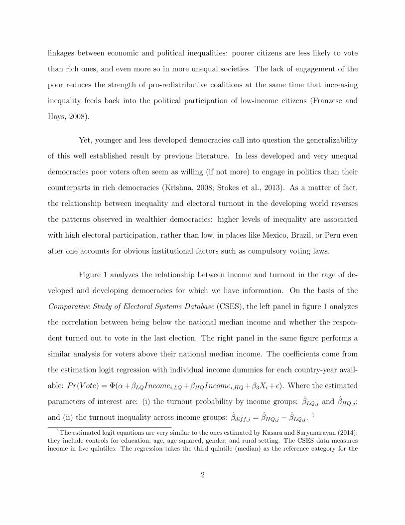
Figure 1 analyzes the relationship between income and turnout in the rage of de-

veloped and developing democracies for which we have information. On the basis of the

Comparative Study of Electoral Systems Database (CSES), the left panel in figure 1 analyzes

the correlation between being below the national median income and whether the respon-

dent turned out to vote in the last election. The right panel in the same figure performs a

similar analysis for voters above their national median income. The coefficients come from

the estimation logit regression with individual income dummies for each country-year avail-

able: Pr(V ote) = Φ(α+βLQIncomei,LQ+βHQIncomei,HQ+β3Xi+ ε). Where the estimated

parameters of interest are: (i) the turnout probability by income groups: βLQ,j and βHQ,j;

and (ii) the turnout inequality across income groups: βdiff,j = βHQ,j − βLQ,j. 1

1The estimated logit equations are very similar to the ones estimated by Kasara and Suryanarayan (2014);they include controls for education, age, age squared, gender, and rural setting. The CSES data measuresincome in five quintiles. The regression takes the third quintile (median) as the reference category for the

2

Figure 1: The Income-Turnout Link across countries

-1 -.5 0 .5 1

Below Median Income Voters

PhilippinesCroatiaTurkeyFrance

BrazilKorea, Republic of

MexicoSwedenFinlandBelarus

SpainUkraineTaiwan

RomaniaCzech Republic

AustriaPolandIreland

IsraelSlovakiaNorway

PeruItaly

BulgariaCanadaHungaryPortugalAustralia

United KingdomAlbania

SwitzerlandGermanySlovenia

IcelandGreece

United StatesDenmark

EstoniaNew ZealandNetherlands

-1 -.5 0 .5 1

Above Median Income Voters

SwedenCroatiaAustria

GermanyNorwayFinland

SlovakiaFrance

SwitzerlandDenmarkCanada

United StatesCzech Republic

AustraliaTurkeySpain

RomaniaIsrael

Korea, Republic ofPortugal

PolandHungaryGreece

BrazilUnited Kingdom

MexicoNetherlandsPhilippines

AlbaniaUkraine

SloveniaIcelandEstoniaTaiwanIreland

ItalyPeru

BulgariaBelarus

New Zealand

Interestingly, there are countries, such as New Zealand, where the middle income

citizens seem more likely to vote than either low or high income ones. There are places like

Sweden, where the low and middle income citizens show very similar patterns of behavior

but high income citizens seem relatively more engaged in elections. There are countries, like

the United States, where the income polarization of turnout is at its maximum: voters in the

bottom half of the income distribution are less likely to vote than the median while at the

same time voters in the top two quintiles are much more likely to do so. And finally there

are countries such as Brazil or Mexico where everyone is nearly as likely to vote: low income

voters do not show a different pattern of behavior relative to either middle or high income

voters.2 The range of variation in the extent to which either low or high income voters differ

impact of the two variables of interest on turnout. Low income quintiles are the bottom two (bottom 40 % ofthe distribution) whereas upper income quintiles include the 4th and the 5th (top 40 % of the distribution).Finally, magnitudes reflect averages within countries for all the years for which there is information availablein the data.

2Importantly, these differences are not a mere reflection of compulsory voting laws. For instance, whileBrazil is known to have effectively enforced compulsory voting laws for literate citizens above 18 and below70, Mexico, Portugal, and France do not. Obviously, we control for this and other institutional features in

3

in their propensity to turn up at the ballot box is quite striking.

Figure 2 presents a summary measure of the levels of political (turnout) inequality

and its relation to economic inequality. Turnout inequality is defined as the difference be-

tween the estimated coefficient for the effect of income on turnout for voters in the top two

quintiles minus the estimated coefficient for the effect of income on turnout for those in the

bottom two quintiles (i.e. βdiff,j = βHQ,j − βLQ,j).3 Economic inequality is measured by the

Gini market coefficient, that is before taxes and transfers.4 Figure 2 brings out a number of

interesting patterns. First, turnout inequality tends to be higher among advanced industrial

than among the middle income countries in our sample. The former are disproportionately

more represented in the upper range of the measure of turnout inequality. The USA show

very high levels of turnout inequality, 5 but so do Germany, Denmark, or Switzerland rela-

tive to the rest of the sample. By contrast, Portugal, Spain, Brazil, Peru, or Mexico have

significantly lower levels than any of these countries.

Second, and more importantly, by considering the relationship between turnout

and the overall distribution of income, figure 2 provides a new perspective on the existing

understanding about the relationship between economic and political inequality. Turnout

inequality tends to be higher in places with intermediate levels of economic inequality. By

contrast, when economic inequality is either very high or very low, turnout inequality de-

clines. What explains these puzzling patterns in the relationship between income and turnout

across nations?

our multivariate analysis below.3Positive values reflect high levels of turnout differentials among voters stratified along income lines.

Negative values imply that low income citizens show a higher propensity to vote than high income citizens(as both are compared to the same reference group, the middle income strata).

4The data are from Solt’s standarized income inequality database (Solt, 2009). We restrict our sampleto the high quality database, that is to estimates with a standard error below 1.5 standard deviations. Thereported patterns are very similar if one uses a post-taxes, post-transfer indicator of inequality instead

5These levels deviate even more with respect to the rest of the sample when one defines turnout in-equality as the ratio between the bottom and the top quintiles of the income distribution (see Kasara andSuryanarayan (2014))

4

Figure 2: Economic and Political (Turnout) Inequality

Albania

AustraliaAustria

Belarus

BrazilBulgaria

Canada

CroatiaCzech Republic

Denmark

Estonia Finland

France

Germany

Greece

HungaryIceland

Ireland

Israel

ItalyKorea, Republic of

Mexico

Netherlands

New Zealand

Norway

Peru

Philippines

Poland

Portugal

Romania

Slovakia

Slovenia Spain

SwedenSwitzerland

Taiwan

Turkey

Ukraine

United Kingdom

United States

-10

12

20 30 40 50 60Inequality (Gini Market Measure)

Largely occupied with the turnout gap by low income citizens in rich countries, es-

pecially the USA, comparative politics has largely neglected the variation in levels of turnout

inequality in the broader range of democracies. While several possible explanations exist to

account for the differences in turnout inequality and turnout decline in rich democracies (e.g.

Blais and Rubenson 2013), the reasons why turnout inequality is low in places like Mexico,

Argentina, Brazil or India and high in societies such as the United States or Germany beg for

additional theoretical and empirical efforts. In two recent and important exceptions, Gallego

(2014) puts the focus on institutional contextual variables, whereas Kasara and Suryanarayan

(2014) stress the importance of the bureaucratic capacity to extract from the rich and the

salience of redistributive conflicts as a political cleavage in societies. In their account, the

rich are more likely to vote than the poor (and therefore turnout inequality is high) when

the threat of extraction is credible (as determined by the level of bureaucratic capacity) and

redistribution (as opposed to alternative second or third dimensions) articulates the contrast

5

between contending political platforms.6

In this paper we pay attention to a different set of mechanisms: parties’ choice of

mobilization strategies to target different groups of voters. We reason from the premise that

turnout levels reflect primarily parties’ efforts to mobilize voters, especially those situated in

the lower half of the income distribution. That the case, the explanation of turnout inequality

requires not only an account of the incentives of high income voters to engage in elections

but also of parties’ choices about (1)whom to target and (2) how to target them. We see these

two choices as interlinked. We explore the conditions under which parties choose to pursue

one of two strategies: mobilization through programmatic party-voter linkages, built around

competitive offerings of sets of public policies (public goods), and mobilization through

clientelistic linkages, which we broadly consider as targeted efforts towards a self-contained

group of voters based on a “particular mode of exchange between electoral constituencies as

principals and politicians as agents [...] focused on particular classes of goods, [...] direct,

contingent” (Kitschelt and Wilkinson, 2007, p.7-8).7

Figure 3 presents a first exploration of the relationship between different forms of

political mobilization and turnout inequality, again measured by βdiff,j = βHQ,j − βLQ,j .8

The type of political mobilization at work in different countries seems highly consequential for

6In an earlier contribution along similar lines, Radcliff (1992) argues that the extent to which economicadversities translates into changes in turnout is mediated by the degree of welfare state development

7For a more detailed analysis of different forms of non-programmatic politics consistent with the approachin this paper see Stokes et al. (2013)

8Clientelism is an aggregate and continuous measure of clientelistic efforts by parties at the country level,codes as b15nwe in Kitschelt’s dataset (Kitschelt, 2013). The aggregate indicator of clientelism reflects thesum (weighted by party size) of experts’ judgment of the extent to which party candidates promise vot-ers (1) consumables (2) benefits or marketable goods (3) access to services or employment (4) governmentcontracts and regulations or any other form of material inducements in exchange for their vote. Similarly,the aggregate indicator for programmatism cosalpo4nwe is also weighted by party size and reflects experts’judgments on the extent to which the coherence and salience of party policy positions are based on severalfundamental dimensions of political competition (social spending on the disadvantaged, state role in govern-ing the economy, public spending, national identity and traditional authority). Both measures are centeredat their mean in the x axis of figure 3. Data points reflect within country averages for all the observation inour data. Bars reflect the standard deviations.

6

Figure 3: Political(Turnout) Inequality and Party Competition

Albania

AustraliaAustria

BrazilBulgaria

Canada

Croatia

Czech Republic

Denmark

EstoniaFinland

France

Germany

Greece

Hungary

Ireland

Israel


Mexico

Netherlands

New Zealand

Norway

Peru

Philippines

Poland

Portugal

Romania

Slovakia

SloveniaSpain

SwedenSwitzerland

Taiwan

Turkey

Ukraine

United Kingdom

United States

-10

12

-2 -1 0 1 2

Clientelism

Albania

AustraliaAustria

BrazilBulgaria

Canada

Croatia

Czech Republic

Denmark

EstoniaFinland

France

Germany

Greece

Hungary

Ireland

Israel


Mexico

Netherlands

New Zealand

Norway

Peru

Philippines

Poland

Portugal

Romania

Slovakia

SloveniaSpain

Sweden Switzerland

Taiwan

Turkey

Ukraine

United Kingdom

United States

-10

12

-2 -1 0 1 2

Programmatism

the observable levels of turnout inequality. There is a strong negative relationship between

clientelism and turnout inequality, and a strong positive relationship between programmatic

competition and turnout inequality. As we will see below, clientelism bolster the political

participation of citizens located in the lower half of the income distribution, thus reducing

turnout inequality. In contrast, programmatism bolsters the participation of citizens in the

upper half, as conflicts over public goods affect them more directly, thus increasing turnout

inequality.

By focusing on parties’ mobilization strategies as the linking mechanism between

economic and political inequality, this paper makes a number of contributions towards a

better understanding of the link between political economy and political behavior. First, by

placing at center stage alternative strategies of party competition, this paper illuminates the

conditions under which elites resort to turnout buying (Nichter, 2008) versus other forms

of policy portfolio diversification (Magaloni, Diaz-Cayeros and Estevez, 2007), and with

7

what consequences. Second, a better understanding of the connection between economic

inequality, party strategies and political inequality helps illuminate the political conditions

under which bad equilibria (high inequality, clientelistic democracies, low state capacity) are

likely to emerge and persist (Robinson and Verdier, 2013). We offer a genuinely political

mechanism behind the persistence of perverse accountability (Stokes, 2005), bad development

equilibria and the self-reproduction of inequality, both economic and political. In doing so,

our analysis expands the array of mechanisms linking affluence and influence (Gilens, 2012;

Gingerich, 2013).

Finally, by exploiting a natural experiment facilitated by the Brazilian federal gov-

ernment’s of randomized audits against corruption at the local level, this paper contributes

to the causal identification of mobilization strategies as the mechanism mediating economic

inequality and electoral turnout. We build on the work by Ferraz and Finan (2008, 2011)

to exploit the audit randomization and gain leverage on the electoral and political conse-

quences of interventions directly designed to curve corruption and clientelism. Through this

approach, we are able to identify the specific conditions under which an exogenous reduc-

tion in the effectiveness of clientelism shifts the relationship between economic and political

inequality.

We find that constraining clientelism through audits translates into larger reduc-

tions in turnout when there are strong local media, when the opposition is stronger, and in

rural as opposed to urban areas. The core of these findings are consistent with recent results

on the impact of audits on vote registration as a mechanism for vote buying (Hidalgo and

Nichter, forthcoming), as well as on the role of local media as transmission mechanisms of

information about the nature of the political process, and their implications for the electoral

fortunes of incumbent political parties (Larreguy, Marshall and Snyder Jr, 2014, 2015). The

rest of the paper is organized as follows. Section I develops our theoretical model. Section II

8

develops the experimental analysis of the randomized corruption audits in Brazilian munici-

palities.Therefore, section III addresses external validity through a large-n analysis. Finally,

section IV concludes and outlines some avenues for further research endeavors.

2 Model: Inequality, Development, and Mobilization

2.1 Premises and Set-up

We model the choice between two policy tools for the purpose of mobilization of

low income voters: targeted goods (that can range from ad hoc transfers (bribes) to small

local club goods) and tax financed public goods (programmatic politics) and study how

inequality shapes the choice of strategy by political elites. The model builds on a number

of assumptions. Parties have limited resources to mobilize voters. They can devote them to

mobilize via targeted good or transfers or programmatic competition. Parties must choose

how much they devote to targeted goods to low income voters (bP ), how much to high

income voters (bR), and how much to general public goods (g). Politics is therefore an

activity initiated by elites at all ends of the ideological spectrum. Accordingly, mobilization

is a choice by different groups of rich citizens. Any subgroup of rich citizens (elite party)

chooses the policy set that maximizes their utility. The fundamental problem for any party

is to maximize the utility of their base such that they attract the support of low income

voters. That is the rich will optimize their policy selection in such a way that they (1)

meet their budget constraint and (2) at least leave the poor indifferent between their policy

offering and the offering that the poor would consider optimal.

To incorporate inequality into the analysis, and following the standard notation in

Acemoglu and Robinson (2006), we define δ and (1− δ) as the fraction of, respectively, rich

9

and poor citizens in any given society. Similarly, we define φ and (1 − φ) as the share of

income of, respectively, the rich and the poor. Using these simple definitions we can express

the income of the rich (wR) and the poor (wP ) as a function of inequality:

wR =φw

δand wP =

(1− φ)w

1− δ

Finally, elites (rulers) face a standard budget constraint defined by tw = bP + bR +

g. To capture the variety of experiences in terms of state/fiscal capacity, we impose the

assumption that a share, λ, of the income of the rich is non-taxable by low income voters.

Accordingly, the budget constraint is defined as:

tw(1− λφ) = bP + bR + g and for the share of citizens (1− δ)

and tw = bP + bR + g for the share of citizens δ

On the basis of these premises, we model the problem as a strategic interaction in which low

income voters decide whether to vote (or not), and the elite parties choose which policy tool

to concentrate their efforts on. Critically, we assume that the poor will vote if their utility

threshold is satisfied by the offerings made by the party of the rich. Therefore, solving the

model requires to take three steps, sequentially:

1. Identify the optimal values of taxes (t∗), private goods (bp), and public goods (g∗) for

the poor, given the budget constraint. These values define the indifference threshold

for the poor to turnout to vote. The problem for low income voters is defined as follows:

maximizet,b,g

Ui(t, b, g) = (1− t)wP + αln(bP ) + g

subject to tw(1− λφ) = bP + bR + g

(1)

10

where α capture the sensitivity of low income voters to targeted goods. As detailed in

the appendix, this yields the following results: b∗P = α; b∗R = 0 ; t∗ = tmax ≤ 1; and

g∗ = tw(1 − λφ) − α. These in turn allow to define the poor voter’s utility threshold

for voting. Poor voters will vote under any combination of t, b, and g that generates

levels of utility at least similar to those defined by:

UP = (1− tmax)wP + αln(α) + tw(1− λφ)− α (2)

This expression defines the level of utility of the poor that the elites must meet with

their policy offerings so that the latter turn out to vote.

2. Identify the optimal values of taxes (t∗), private goods (br), and public goods (g∗)

for the elite. The elites, irrespective of their ideological leanings, needs to choose a

portfolio of targeted goods, public goods, and taxes that meets two constraint: (1) a

budget constraint (recall that the poor had limited ability to tax the elite, but the

elite has full capacity to tax itself); and (2) a political constraint driven by the need

to meet the mobilization threshold of low income voters defined in (2). Accordingly,

its maximization problem can be defined as:

maximizet,b,g

Ui(t, b, g) = (1− t)wR + βln(bR) + g

subject to tw = bP + bR + g

and to (1− t)wP + αln(bP ) + g ≥ UP

(3)

where β captures the sensitivity of high income voters to targeted goods and UP defines

the low income voters’ utility threshold as defined above.

3. Study how inequality shapes the choice of strategy and establish the equilibria resulting

from the strategic interaction between rich and poor citizens.

11

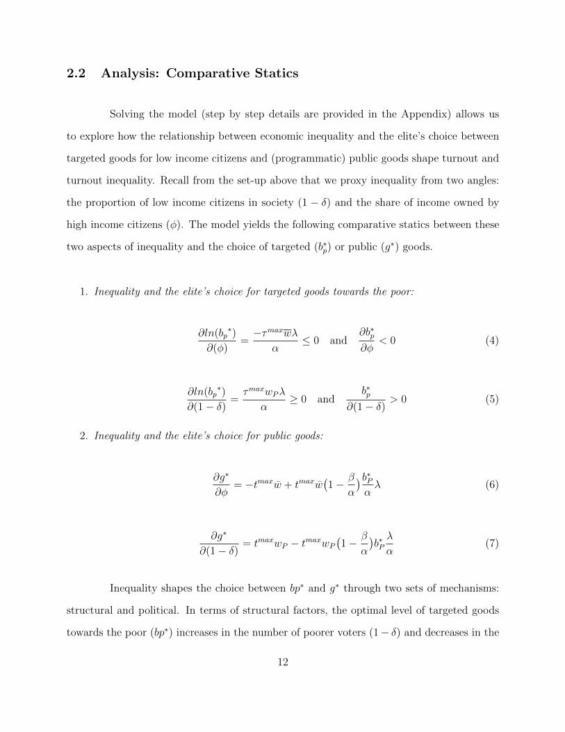
2.2 Analysis: Comparative Statics

Solving the model (step by step details are provided in the Appendix) allows us

to explore how the relationship between economic inequality and the elite’s choice between

targeted goods for low income citizens and (programmatic) public goods shape turnout and

turnout inequality. Recall from the set-up above that we proxy inequality from two angles:

the proportion of low income citizens in society (1 − δ) and the share of income owned by

high income citizens (φ). The model yields the following comparative statics between these

two aspects of inequality and the choice of targeted (b∗p) or public (g∗) goods.

1. Inequality and the elite’s choice for targeted goods towards the poor:

∂ln(bp∗)

∂(φ)=−τmaxwλ

α≤ 0 and

∂b∗p∂φ

< 0 (4)

∂ln(bp∗)

∂(1− δ)=τmaxwPλ

α≥ 0 and

b∗p∂(1− δ)

> 0 (5)

2. Inequality and the elite’s choice for public goods:

∂g∗

∂φ= −tmaxw + tmaxw

(1− β

α

)b∗Pαλ (6)

∂g∗

∂(1− δ)= tmaxwP − tmaxwP

(1− β

α

)b∗Pλ

α(7)

Inequality shapes the choice between bp∗ and g∗ through two sets of mechanisms:

structural and political. In terms of structural factors, the optimal level of targeted goods

towards the poor (bp∗) increases in the number of poorer voters (1− δ) and decreases in the

12

share of income of the upper half (φ). The former effect captures the strategic implications

of a change in the size of the pool of potentialy targetable voters. Insofar as the poor are

relatively more reponsive to targeted goods than the elite, an increase in the share of low

income citizens makes rational for elites to increase efforts in clientelistic mobilization and

reduce the supply of public goods. he latter captures the fact that as elites become wealthier,

it is cheaper for them to buy votes. Interestingly,our result above also implies that the elites

will shift away from clientelism to a larger extent as development increases, a result consistent

with previous findings in the literature (Kirchheimer, 1965).

More interestingly, our results point to an important political mechanism: namely,

the ability of the elite to hide away part of their wealth (and conversely the ability of the

state to monitor and tax). A higher ability of the rich to hide their wealth (λ) enhances

both the rationality of clientelism when the number of poor increases and the shift away from

clientelism as development increases. By contrast, at later stages of political development,

when elites cannot hide away their wealth (λ = 0), an increase in the number of the poor

does not lead to increasing clientelistic efforts (rather it leads to more public goods), and an

increase in the elite’s wealth yields a lower provision of public goods (which they would have

to fund).

These results unveil the strategic calculus of elites. Elites do not only react by

mobilizing against the increasing revenue raising power of the state (as in Kasara and Surya-

narayan (2014)). They actually lead and anticipate different political scenarios through their

choice of mobilization technology. Our model identifies the conditions under which clien-

telism is rational and self-enforcing9, namely low development, high inequality and a political

constraint on the ability of the state to prevent elites from hiding part of their wealth (low

state capacity), at the expense of the provision of public goods and programmatic competi-

9Thus preventing endogenously in the first place the rise in state capacity that would lead upper incomegroups to mobilize against the state

13

tion10. To see this let us consider what happens to the choice of policy offerings when the

elite is not constrained to meet the utility threshold that ensures the participation of the

poor. To this end, we solve the elite’s problem with and without the political constraint

(U) and evaluate the difference between the two. This analysis yields the following results

(again, full details in Appendix):

g∗ > g∗U if β < α and b∗p > 0 (8)

The comparison outlined in [8] suggests an important result: insofar as the poor

are more responsive to targeted goods than the rich and b∗p > 0, both conditions that occur

precisely under conditions of high inequality, meeting the political constraint of the poor

implies a sacrifice in terms of public goods. Under conditions of high inequality and low tax

capacity11, it is both necessary and cost efficient to meet the political constraint of the poor

to win elections and therefore privileging b∗p becomes the optimal strategy. Insofar as the

number of poor and the optimal size of targeted goods towards decline, elites will tend to

resort to public goods as the key policy device to win elections.

To summarize, elites will resort to clientelism as opposed to public goods when they

have the capacity to hide part of their income from taxes, the share of low income citizens is

large, their income is low and as a result they are responsive to bribes in a society with lower

average income. We refer to this scenario as a high inequality, lesser development equilibrium

in which low income voters respond to elite’s clientelistic strategies, thereby leading to higher

levels of turnout and reducing the level of observable turnout inequality. By contrast, when

the state can actually limit the ability of elites to hide their income, the income of the poor

10For evidence consistent with this theoretical contention in the Brazilian case, see Timmons and Garfias(2015)

11See Besley and Persson (2011) for a discussion of some of the mechanisms through which high inequalityand low tax capacity reinforce each other

14

is higher, and societies are relatively wealthier, elites find clientelism increasingly expensive

and suboptimal relative to the provision of public goods. As this dynamics consolidates, a

different scenario around programatic competition emerges, one in which societies are more

developed and relatively more equal, low income citizens are less targeted as such, leading

to lower levels of turnout and higher levels of turnout inequality.

The joint consideration of these two scenarios suggest that the level of inequality

and the nature of political competition jointly determine the level of turnout inequality,

which leads to the following hypothesis: Conditional on economic inequality being sufficiently

high, clientelism (programmatism) increases (reduces) the level of turnout, thus reducing

(increasing) the level of turnout inequality. In addition, our argument also implies that the

specific combinations of inequality and mobilization constitute an equilibrium, the symmetric

conditional relationship should also hold: given clientelism (programmatism) as the dominant

form of political competition, higher economic inequality increases (reduces) the level of

turnout of low income voters, thus reducing (increasing) turnout inequality.

3 Empirical Strategy

Needless to say, causally identifying this relationship poses major challenges. Sev-

eral recent contributions highlight various feedback channels, further enhancing the challenge

of causally identifying the mechanism posited in this paper. Fergusson, Larreguy and Ri-

ano (2014) show how parties with a strategic advantage in clientelistic politics will oppose

investments in state capacity, thus limiting pro-equality politics. Debs, Helmke et al. (2010)

show that the left fares better under equality because voters are more likely to cling to pro-

redistributive coalitions that in turn help contain inequality. Bursztyn (2013) focuses in turn

on voter’s demand: it is the voters themselves who may not want more public goods under

15

conditions of high inequality and high turnout, thus reinforcing the vicious circle. Finally,

incorporating several of these mechanisms into a common framework, Robinson and Verdier

(2013) show how clientelism becomes self-enforcing under conditions of high inequality and

low productivity. If clientelism feeds back into inequality (and viceversa), it is hard to imag-

ine a situation in which mobilization strategies change for exogenous reasons, thus allowing

to identify its mediating role between economic and political inequality.

To ameliorate these concerns, we follow in the footsteps a recent stream of scholar-

ship exploiting Brazilian municipalities as source of leverage to identify mechanisms driving

the interaction between voters and politicians in contexts with a strong incidence of cor-

ruption, clientelism, and inequality (Hidalgo and Nichter, forthcoming; Brollo, 2012; Brollo

et al., 2013). Our specific strategy focuses primarily on the random audits by the Brazilian

government on its municipalities (Ferraz and Finan, 2008). The federal audits on Brazilian

municipalities constitute an excellent case for three reasons: first, these audits, implemented

through a randomized selection of targeted municipalities, provide a plausibly exogenous

manipulation of that effectiveness of clientelistic political competition that gives us signifi-

cant methodological leverage; second, in terms of linking concepts and measurement, insofar

as clientelism and the ability of the rich to hide their wealth go hand in hand, the available

proxy for clientelism (details below) captures directly the extent to which local elites manage

to privatize wealth both for private gains and for political purposes; third, the audits provide

a good balance between internal and external validity in that they cover a large number of

municipalities with sufficient variation in terms of our key parameters of interests, namely

inequality and political mobilization strategies.

Admittedly, though, our empirical strategy faces a trade-off between identification

leverage and measurement accuracy. While the data on audits provides the former, we do

not have a direct measure of turnout inequality at the local level in Brazil. Instead, our

16

empirical strategy rests on the premise that in contexts such as Brazil aggregate turnout

rates provide relevant information on the behavior of low income voters. In support of our

premise, recent findings by Cepaluni and Hidalgo (forthcoming) suggest that this very much

depends of the type of intervention (and their associated penalties) being evaluated. When

the penalties associated with the intervention affect services with access primarily reserved to

middle and upper income groups, changes in turnout rates will reflect the elasticity of these

groups to the intervention (in their case, age related enforcement of compulsory voting).

When the intervention affects instruments such as mismanagement of cash funds or access

to basic social services, as it is the case with the anti-corruption audits, the expectation is

that aggregate turnout rates trace in large part responsiveness by lower income strata.

At the other end of the trade-off, we perform a large n analysis a large n multilevel

cross-national analysis of the determinants of turnout inequality as defined in figure 2). This

exercise helps assess whether the relationship between economic and political inequality

follows the patterns suggested by our theory more broadly, after we have provided plausible

causal evidence on the workings of a key mechanism behind it. In addition, it allows us to

establish the robustness of our results with a measure of turnout levels and turnout inequality

that captures directly the behavior of voters at different levels of income.

4 Evidence from Brazil

We proceed in two steps: first, we describe the institutional background of the case

study and outline our research design; second, we present the econometric specifications to

best exploit the quasi-experimental nature of the data and discuss the findings.

17

4.1 Institutional Background and Research Design

The ability to identify the impact of an exogenous change in party strategies derives

from two major institutional innovations introduced by Brazilian authorities since the late

1990s (Ferraz and Finan, 2008, 2011). The first consists in a constitutional change to allow

the possibility of re-election at the local level in 1997, implemented from the 2000 elections

onwards; the second, in the launch of a major anticorruption initiative in 2003, led by

the Controladoria General da Uniao (CGU), scrutinizing the use of federal funds by local

authorities. The audit analyzes the use of federal funds by localities during the period

2001-2004. These data allow us to to do three things:

1. Make use of various measures of the extent to which local authorities resort to clien-

telistic strategies in the run-up to the election (or re-election). To measure party

strategies we resort to the variable that Ferraz and Finan (2011) defined as local mis-

management and that is defined as “the number of violations divided by the number of

service items audited” (Ferraz and Finan, 2011, p. 1284). These violations include the

performance of uncompetitive bidding for local contracts, the misuse of resources for

earmarked for other purposes (i.e. using resources intended for health to boost teachers

salaries) or other forms of turning public goods into club goods.This proxy matches

quite closely the conceptualization of clientelistic strategies as a “material inducement”

geared towards the modification of electoral behavior that defines clientelism(Kitschelt

and Wilkinson, 2007). 12

2. Match these measures to census-based socio-demographic, and economic information

at the local level, as well as to detailed political information obtained from the Tribunal

12Results below are robust to replacing this indicator by proxies capturing acts of corruption more directlyoriented towards targeted personal gains, such as frauds in procurement, diversions of public funds to privateindividuals or entities, or over-invoicing of goods and services.

18

Superior Electoral (TSE), including the level of turnout in local elections. While in

Brazil there are compulsory voting laws in place for individuals between 18 and 70

in all elections, there remains considerable variation in the average levels of turnout

across localities. For the localities in our sample, the range was between 65% and 96%

in 2000 and 2004. In both instances the distribution was approximately normal (see

Figure 10 in the Appendix). If anything, the reduced variation due to institutional

constraints makes Brazil a harder case to test the hypothesis.

3. Evaluate whether truly exogenous changes in the type of political strategy adopted by

local elites matter for changes in the level of turnout at different levels of inequality.

The leverage for our identification strategy emerges from several features of the

design and implementation the anti-corruption program by the Brazilian federal authority.

These features are as follows (see Ferraz and Finan (2011, 2008) for additional details on the

program):

1. Through a sequence of lotteries, the CGU chose randomly about 8% of a total of

5500 Brazilian municipalities, including state capitals and coastal cities (N of audited

municipalities=366). Once a municipality is chosen, the CGU gathers information on

all federal funds received and sends a team of auditors to examine the use of these

funds (particularly in the areas of public works and public services). Auditors get

information from the community and the local council members about any form of

malfeasance or misuse of funds, as well as from the local documentation available.

2. Immediately, after the inspection (about a week long visit), a detailed report is sent

back to the CGU, which in turn forwards it to the federal accounting auditor (Tri-

bunal de Contas da Uniao), the judiciary, and all members of the local council. A

19

summary with the key findings for each audited municipality is made available online

and disclosed to local media.

3. Critically, we have information on the date in which the reports were released to parties

and voters. As a result we can exploit the contrast between those municipalities in

which the audit results were released before the 2004 election and those in which they

were not. Since the sequence selection-inspection-release is standard across all the

audits and takes a similar amount of time once the municipality is randomly chosen,

we can rule out the possibility of strategic releases by the federal government in the

run-up to the 2004 election. Given the short time span between selection, visit, and

release randomization determines both which particular municipality is selected and

when the information is released.

The combination of the random selection of municipalities and the discontinuity

around the 2004 election define both the nature of the treatment and the composition of the

treatment and control groups. Since all the municipalities included in our sample have been

investigated, the treatment is whether the results of the audit have been made public to local

citizens and competing parties or not. It is therefore a purely informational treatment in

which the treatment group includes all municipalities that have been audited and in which

the results of the investigation have been released and the control group includes all the

municipalities where the investigation took place and was released after the 2004 election.

See Table 5 in the Appendix to see the balance tables for the treatment and control groups.

Our approach implies that the publication of the audit reports undermines the

feasibility of clientelism as a mobilization strategy. Accordingly, we should observe that,

given high levels of inequality, in those municipalities where the publication of the audit

induces a switch towards more programmatic political competition, clientelism ceases to be

20

a viable mobilization strategy and higher levels of inequality are associated with a reduction

in the levels of turnout in the next election. Before describing the main results (that to

changes in turnout), it is worthwhile mentioning that Table 3 in the Appendix shows that the

(ex-post) audited mismanagement interacted with inequality was already a good predictor

of the turnout levels in 2000.

4.2 Specification and Findings

To establish weather these expectations are borne out by the data, we model the

determinants of the change in the levels of turnout between 2000 and 2004 13 as a function of

the interaction between three variables: the degree of inequality within the municipality, as

measured by Brazil’s census bureau, the type of political strategy adopted (more local mis-

management implies more clientelism, and viceversa), and a dummy capturing whether the

municipality belongs to the treatment or the control group (before vs after 2004). To keep

the comparison as sharp as possible we restrict the sample to those majors who just finished

their first mandate and are seeking re-election for the first time.14. In addition, merging

and expanding the databases in Ferraz and Finan (2011) and Ferraz and Finan (2008) to

include all relevant potential confounders, we introduce controls concerning municipal level

characteristics15, specific political and judicial institutions 16 , the level of federal transfers

received and the level of unemployment within the municipality, mayor specific characteris-

13Specifically, the change in turnout is defined as 4T = T2004−T2000

T2000.

14In the appendix (table 4) we provide evidence that the higher the number of terms a major has beenin office, the more he/she tends to resort to clientelistic practices. Therefore, this restriction is in order toavoid the confounding effect of the length of term in office.

15Gathered from either the CGU or the Instituto de Pesquisa Economica placed (IPEA), these include:the area, the log of population, the share of urban population within the municipality, the local gdp percapita, the change in the level of population between censuses, the share of population over 18 with at leastsecondary education, whether the municipality is new, the number of active public employees.

16These include whether the municipality has a judicial district, whether the municipality used participa-tory budgeting during the period 2001-2004, and the seats (vereadores) to voters ratio within each munici-pality

21

tics17, electoral competition18, and the change in the electoral census. The results are robust

to the inclusion to controls for all these potential confounders, as well as to the inclusion of

lottery fixed effects and state level fixed effects. 19

Table 1 displays the full battery of specifications. All models include lottery fixed

effects (FEs) to account for different timing in the audit release 20. Columns 1 and 2 do

not include regional fixed effects, whereas all the other columns include them. Since we

know that clientelism is geographically concentrated among certain areas, the inclusion of

regional FEs is important. And also, the inclusion of regional FEs provides some safety net

against unobserved heterogeneity. Finally, the last two columns exclude those municipalities

in which the mayor was member of the PMDB. The reason is that the PMDB is known for

being one of the parties with powerful clientelistic machines.

The results are pretty much stable across all the specifications in Table 1. It is

remarkable that the results are robust to the inclusion of both mayor’s characteristics controls

and to regional fixed effects. Audits information release had a negative effect on turnout

especially when both the audited mismanagement and inequality were high. However, the

results are specially strong once the incumbents who are members of the PMDB are excluded

in the last two columns. This might be explained by the fact that PMDB’s mayors may have

devoted resources to exonerate them after the audit releases 21.

17Including age, gender, level of education, and past non-consecutive experience as a mayor or councilmember.

18Gathered primarily from the TSE these include the share of council members from the same party asthe major, whether the major was from the same party as the governor, the effective number of parties inthe 2000 election, and the margin of victory.

19Importantly, we have also checked if the correlation between mismanagement and inequality is thesame across exposed and non exposed municipalities. To do so we have estimated several regressions withinequality prior to 2004 as dependent variable and the interaction between mismanagement and exposure(i.e. the treatment) as independent variables; controlling for the municipality characteristics and regionalfixed effects. In such models the null hypothesis according to which for both the treatment (exposed) andcontrol groups (non exposed) there is no effect of audited mismanagement on inequality cannot be rejected.

20In addition, standard errors are clustered at the region (state) level.21Interestingly, with the sample that excludes the PMDB mayors, the model without any controls also

provides significant results.

22

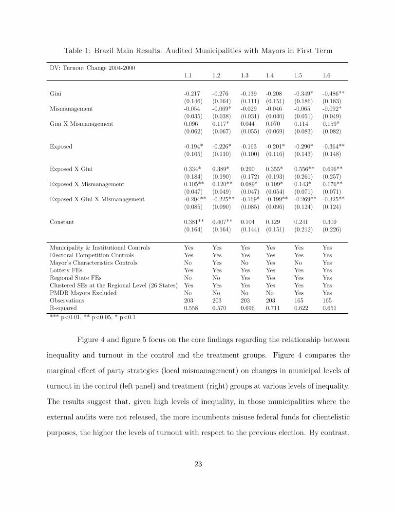
Table 1: Brazil Main Results: Audited Municipalities with Mayors in First Term

DV: Turnout Change 2004-20001.1 1.2 1.3 1.4 1.5 1.6

Gini -0.217 -0.276 -0.139 -0.208 -0.349* -0.486**(0.146) (0.164) (0.111) (0.151) (0.186) (0.183)

Mismanagement -0.054 -0.069* -0.029 -0.046 -0.065 -0.092*(0.035) (0.038) (0.031) (0.040) (0.051) (0.049)

Gini X Mismanagement 0.096 0.117* 0.044 0.070 0.114 0.159*(0.062) (0.067) (0.055) (0.069) (0.083) (0.082)

Exposed -0.194* -0.226* -0.163 -0.201* -0.290* -0.364**(0.105) (0.110) (0.100) (0.116) (0.143) (0.148)

Exposed X Gini 0.334* 0.389* 0.290 0.355* 0.556** 0.696**(0.184) (0.190) (0.172) (0.193) (0.261) (0.257)

Exposed X Mismanagement 0.105** 0.120** 0.089* 0.109* 0.143* 0.176**(0.047) (0.049) (0.047) (0.054) (0.071) (0.071)

Exposed X Gini X Mismanagement -0.204** -0.225** -0.169* -0.199** -0.269** -0.325**(0.085) (0.090) (0.085) (0.096) (0.124) (0.124)

Constant 0.381** 0.407** 0.104 0.129 0.241 0.309(0.164) (0.164) (0.144) (0.151) (0.212) (0.226)

Municipality & Institutional Controls Yes Yes Yes Yes Yes YesElectoral Competition Controls Yes Yes Yes Yes Yes YesMayor’s Characteristics Controls No Yes No Yes No YesLottery FEs Yes Yes Yes Yes Yes YesRegional State FEs No No Yes Yes Yes YesClustered SEs at the Regional Level (26 States) Yes Yes Yes Yes Yes YesPMDB Mayors Excluded No No No No Yes YesObservations 203 203 203 203 165 165R-squared 0.558 0.570 0.696 0.711 0.622 0.651

*** p<0.01, ** p<0.05, * p<0.1

Figure 4 and figure 5 focus on the core findings regarding the relationship between

inequality and turnout in the control and the treatment groups. Figure 4 compares the

marginal effect of party strategies (local mismanagement) on changes in municipal levels of

turnout in the control (left panel) and treatment (right) groups at various levels of inequality.

The results suggest that, given high levels of inequality, in those municipalities where the

external audits were not released, the more incumbents misuse federal funds for clientelistic

purposes, the higher the levels of turnout with respect to the previous election. By contrast,

23

Figure 4: Marginal Effect of Local Mismanagement on Change in Turnout

-.05

-.03

-.01

.01

.03

.05

.45 .5 .55 .6 .65 .7 .75 .45 .5 .55 .6 .65 .7 .75

Not Exposed Exposed

Gini Municipality Gini Municipality

in those municipalities where the audit took place and was released before the 2004 election,

the same strategy triggers a reduction in electoral participation of a similar magnitude. For

completion, Figure 11 in the Appendix shows the marginal effect of inequality on changes in

turnout for the treatment and control groups. The results further reinforce our theoretical

expectations: higher levels of inequality translate into lower levels of turnout when the

audited mismanagement is low in the control group. But crucially the relationship reverses

for the treatment group: more inequality leads to less turnout when high levels of clientelism

has been exposed and, we argue, they are no longer effective prior to the election.

We take this to be evidence that when a political shift towards programmatism is

exogenously induced, clientelism ceases to be an effective mobilization strategy (again) under

high levels of inequality. Figure 5 digs deeper by displaying the heterogenous effects of the

treatment, namely an actual exposure to random audits. Under a status quo of low inequality

and relative programmatism (i.e. low levels of mismanagement of federal funds), the results

24

Figure 5: Marginal Effect of Random Audit Exposure on Change in Turnout

-.2

-.1

0.1

.2.3

0 1 2 3 4 5 6

Mismanagmenet Audited

Low Inequality

0 1 2 3 4 5 6

Mismanagmenet Audited

High Inequality

suggest (falls just short of statistical significance) that exposure of the audit results may

have demobilized voters, thus reducing the level of turnout. Interestingly, though, under

conditions of high inequality and rampant clientelism, exposure of political actors to random

audits has a clear and significant demobilization effect.

The quasi-experimental results on the basis of random audits of Brazilian munici-

palities lend strong a robust support to the idea that party strategies mediate the relationship

between economic inequality and electoral turnout. Under clientelism (proxied by high lev-

els of local mismanagement) more inequality is associated with higher levels of turnout (and

by implication less turnout inequality). By contrast, the exogenous reduction in the effec-

tiveness of clientelism enforced by randomly the federal audits, switches the nature of the

relationship between inequality and turnout: once clientelism is no longer effective, higher

levels of inequality lead to lower levels of turnout, and by implication to higher levels of

turnout inequality.

25

4.3 The Mechanism: Limits on Clientelism

The results in the previous section are both robust and consistent with the hy-

pothesis. To further substantiate the idea that the randomized audits exogenously reduced

the effectiveness of clientelism, thus altering the connection between economic and political

inequality, this section presents additional analyses that delve deeper in the nature of the

mechanism triggered by the audits and their exposure. We focus first on the informational

nature of the treatment by comparing municipalities with strong local media presence (radio

or newspaper 22) to those without it. If the information effect we attribute to the exposure

of the audits is real, the transformation of the relationship between inequality and turnout

should be particularly visible in areas with strong local media presence. Figure 6 (and

the corresponding table 6 in the Appendix) examine the contrast in the effect of audits in

municipalities with and without a strong local media presence.

Second, to the extent that audits render clientelism less feasible and less effective,

their impact should be all the more visible in areas with a strong and effective opposition

capable of capitalizing politically on the diffusion of the audits results and, more impor-

tantly, of keeping an eye on attempts by incumbents to keep on misusing federal funds for

political purposes. To assess this possibility, Figure 7 (and the corresponding table 7 in

the Appendix) explore the heterogenous treatment effects of the audits on the relationship

between inequality and turnout across two subgroups of municipalities: those where the

margin of victory in the 2000 election was below on standard deviation and those where

the same margin was above, indicating that the incumbent had secured a stronger politi-

cal victory. Finally, if audits really worked to constrain the feasibility of clientelism, their

ability to modify the relationship between economic and political inequality should be more

22See Ferraz and Finan (2011) for the coding of the variable distinguishing whether localities had au-tonomous media.

26

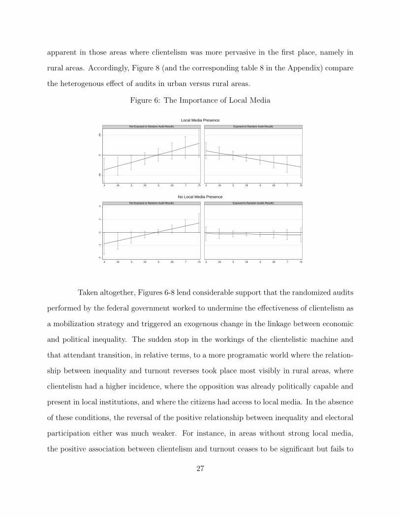
apparent in those areas where clientelism was more pervasive in the first place, namely in

rural areas. Accordingly, Figure 8 (and the corresponding table 8 in the Appendix) compare

the heterogenous effect of audits in urban versus rural areas.

Figure 6: The Importance of Local Media-.

050

.05

.4 .45 .5 .55 .6 .65 .7 .75 .4 .45 .5 .55 .6 .65 .7 .75

Not Exposed to Random Audit Results Exposed to Random Audit Results

Local Media Presence

-.4

-.2

0.2

.4

.4 .45 .5 .55 .6 .65 .7 .75 .4 .45 .5 .55 .6 .65 .7 .75

Not Exposed to Random Audit Results Exposed to Random Audits Results

No Local Media Presence

Taken altogether, Figures 6-8 lend considerable support that the randomized audits

performed by the federal government worked to undermine the effectiveness of clientelism as

a mobilization strategy and triggered an exogenous change in the linkage between economic

and political inequality. The sudden stop in the workings of the clientelistic machine and

that attendant transition, in relative terms, to a more programatic world where the relation-

ship between inequality and turnout reverses took place most visibly in rural areas, where

clientelism had a higher incidence, where the opposition was already politically capable and

present in local institutions, and where the citizens had access to local media. In the absence

of these conditions, the reversal of the positive relationship between inequality and electoral

participation either was much weaker. For instance, in areas without strong local media,

the positive association between clientelism and turnout ceases to be significant but fails to

27

Figure 7: The Strength of the Opposition

-.1

-.05

0.0

5

.4 .45 .5 .55 .6 .65 .7 .75 .4 .45 .5 .55 .6 .65 .7 .75


Strong Opposition (Win Margin in Previous Election < 1 Std Deviation)

-.2

-.1

0.1

.2

.4 .45 .5 .55 .6 .65 .7 .75 .4 .45 .5 .55 .6 .65 .7 .75


Weak Oppositin (Win Margin in Previous Election > 1 Std Deviation)

Figure 8: Urban vs Rural Environments

-.1

-.05

0.0

5

.4 .45 .5 .55 .6 .65 .7 .75 .4 .45 .5 .55 .6 .65 .7 .75


Rural Areas

-.06

-.04

-.02

0.0

2

.4 .45 .5 .55 .6 .65 .7 .75 .4 .45 .5 .55 .6 .65 .7 .75


Urban Areas

28

fully reverse. In turn, in the case of areas with a weak opposition, the exposure to audits

eliminates the positive impact of clientelism on turnout but does not turn the relationship

into a negative one, as happens in areas with a strong opposition. A similar situation is

observable in cities as opposed to rural areas.

5 External Validity: Comparative Evidence

Our argument implies that a switch to programmatism in countries with high in-

equality causes a relative demobilization of low income voters that reduces overall levels of

turnout and increases turnout inequality. While the previous section has identified the effect

of an exogenous change in the type of political mobilization and has provided evidence on the

mechanisms at work, the available data constrain us to study only the implications of such

changes on the overall levels of turnout. That is, the study of the determinants of turnout

across Brazilian municipalities does not rest on a direct measure of the behavioral responses

by low income voters to different combinations of inequality and clientelism/programmatism.

To overcome this limitation and assess the external validity of our logic, Table 2 analyzes

the determinants of both low income voters turnout (columns 1-3) and the corresponding

levels of turnout inequality (columns 4-6).

We perform a two-stage analysis (Lewis and Linzer, 2005) 75 country-year surveys

from the Comparative Study of Electoral systems (Waves 1, 2, & 3). The first stage23

analysis produces the measure of turnout inequality presented in Figure 2, which we then

use as the dependent variable in the second stage. In the second stage we implement a FGLS

estimator to account for heterokedasticity since the dependent variable in the first stage is

23Recall that the first stage estimates the logit regression Pr(V ote) = Φ(α + βLQIncomei,LQ +βHQIncomei,HQ +β3Xi + ε) in each country-year available across the three CSES waves; where the controlsincluded are age, age squared, education, gender, and a dummy variable capturing urban-rural divides.

29

not estimated with the same precision in all the available country-surveys from the CSES

data. Accordingly, the second stage models recover the standard error from the first stage

and implements the Borjas correction in the second stage, weighting the second stage models

by the standard errors of the individual level.24 The key independent variable of interest is

again the level of economic inequality in interaction with the clientelistic efforts. We use the

Gini coefficient after taxes and transfers for the former 25 and the same measure of political

parties’ clientelistic efforts reported in figure 3.

A first set of controls include potential confounders associated with structural socio-

economic variables 26 (some of which could potentially shape electoral behavior via economic

voting). A second set of controls targets the institutional determinants of turnout among

low income people: a first, and obvious one, concerns whether the country has compulsory

voting legislation. In addition, the degree of institutionalization of democracy, as captured

by Polity, captures socialization effects; the electoral system holds constant institutional

features that constrain the role of parties as mediators between the executive and the voters.

In addition, the amount of redistribution in place in any given country/year, controls for

the opportunity cost of not voting for low income citizens. Finally, we also control for other

features that may impact the incentives of low income voters to engage in politics such as

the degree of ethnic fractionalization and the infant mortality rate (included as a proxy of

the specific incidence of low levels of development on the very poor). 27

The findings reported in table 2 are fully consistent with the expectations derived

24In addition, the second stage models are clustered at the country-level since we have multiple CSESwaves for various countries.

25The data are from Solt’s standarized income inequality database (Solt, 2009). We restrict our sampleto the high quality database, that is to estimates with a standard error below 1.5 standard deviations.

26These include: Population size, GDP per capita (both logged), GDP growth, and the economic global-ization index.

27All controls are mean centered and standardized so that they take values between 0 and 1. The sourcesof the cross-country variables is the Quality of Government Institute Dataset (v.2013) and the Penn WorldTables.

30

Table 2: Cross Section: Second Stage Regressions, Clientelism Measure

Second Stage Weighted Regressions Low-Income Voters Turnout βLQ,j Turnout Inequality βdiff,j2.1 2.2 2.3 2.4 2.5 2.6

Gini Net -0.517** -0.431*** -0.639** 0.359* 0.359* 0.754**(0.220) (0.154) (0.283) (0.211) (0.180) (0.349)

Clientelism -0.639*** -0.535*** -0.671* 0.495** 0.501*** 0.831**(0.219) (0.161) (0.344) (0.183) (0.167) (0.378)

Gini Net X Clientelism 1.064** 0.937*** 1.312** -0.893** -0.878*** -1.599**(0.398) (0.284) (0.542) (0.342) (0.306) (0.645)

High Income Voters Turnout (βHQ,j) 0.569*** 0.571*** 0.316** 0.287*(0.091) (0.099) (0.120) (0.156)

Constant -0.010 -0.083 -0.091 0.117 0.093 0.117(0.141) (0.149) (0.174) (0.161) (0.153) (0.176)

Controls Yes Yes Yes Yes Yes YesBorjas Weighting Yes Yes Yes Yes Yes YesClustered Std Errors at the Country Level Yes Yes Yes Yes Yes YesHigh Quality Gini Dataset (Solt 4.0) Yes Yes Yes Yes Yes YesClientelism Data Time Trend Correction No No Yes No No YesCSES Waves 1,2&3 1,2&3 1,2&3 1,2&3 1,2&3 1,2&2Countries 30 30 25 30 30 25Observations (Country-Year) 75 75 47 75 75 47R-squared 0.293 0.544 0.514 0.638 0.698 0.674Controls Include: lnGDPpc, Redistribution, Compulsory Voting, PR, lnPOP, Polity2, Mortality Rate, GDP Growth, Globalization Index

*** p<0.01, ** p<0.05, * p<0.1

from the model as well as with the experimental evidence reported in the previous section.

Given high levels of economic inequality, clientelism works to increase the level of turnout

by low income voters (columns 1-3) -i.e. when the dependent variable is βLQ,j. Conversely,

programmatism shows the opposite effects (see Table 9 in the Appendix). Figure 9 displays

the predicted behavior of low income voters at different combinations of economic inequality

and political mobilization strategies. The cross-national patterns show remarkable consis-

tency with the ones identified in the case of Brazilian municipalities using the overall levels

of turnout as the dependent variable: given high levels of economic inequality, clientelism

(programatism) increases (reduces) the political engagement of low income voters. On the

other hand, columns 4 to 6 show in turn how the behavior of low income voters translates

into the overall patterns of turnout inequality (βdiff,j). Interestingly, these results are ro-

31

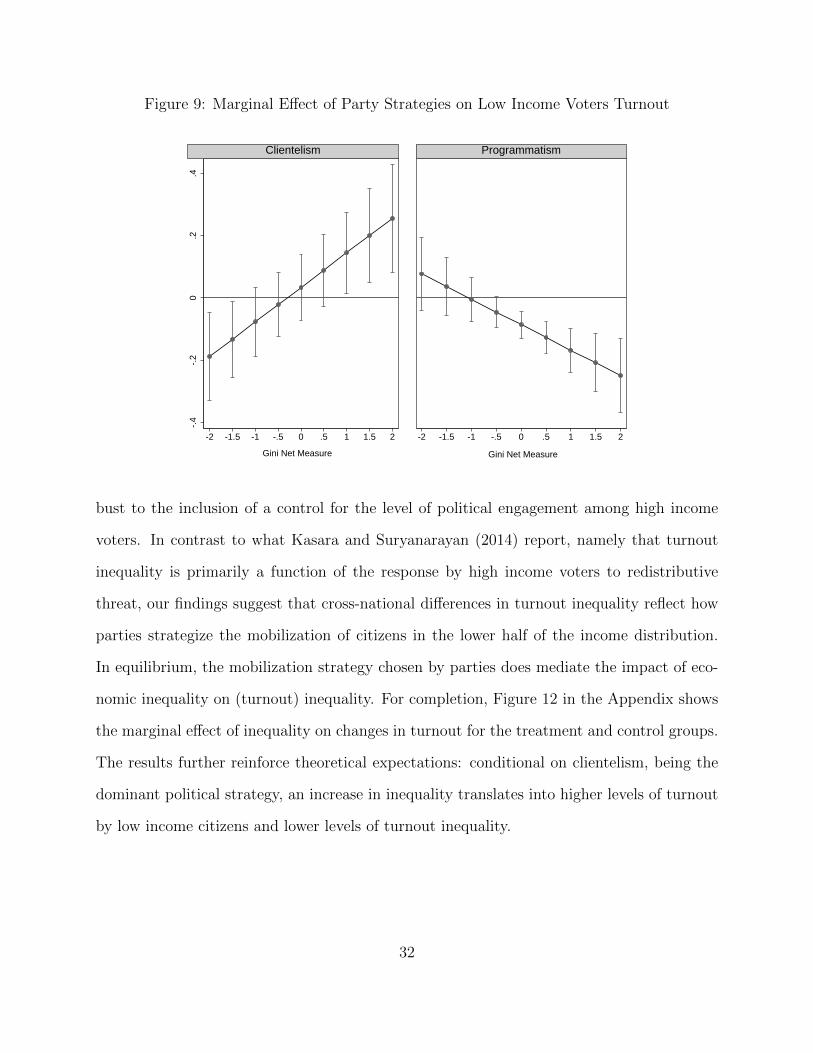
Figure 9: Marginal Effect of Party Strategies on Low Income Voters Turnout

-.4

-.2

0.2

.4

-2 -1.5 -1 -.5 0 .5 1 1.5 2

Gini Net Measure

Clientelism

-2 -1.5 -1 -.5 0 .5 1 1.5 2

Gini Net Measure

Programmatism

bust to the inclusion of a control for the level of political engagement among high income

voters. In contrast to what Kasara and Suryanarayan (2014) report, namely that turnout

inequality is primarily a function of the response by high income voters to redistributive

threat, our findings suggest that cross-national differences in turnout inequality reflect how

parties strategize the mobilization of citizens in the lower half of the income distribution.

In equilibrium, the mobilization strategy chosen by parties does mediate the impact of eco-

nomic inequality on (turnout) inequality. For completion, Figure 12 in the Appendix shows

the marginal effect of inequality on changes in turnout for the treatment and control groups.

The results further reinforce theoretical expectations: conditional on clientelism, being the

dominant political strategy, an increase in inequality translates into higher levels of turnout

by low income citizens and lower levels of turnout inequality.

32

6 Conclusion

This paper has developed an explanation of turnout inequality based on the in-

teraction between economic inequality parties’ mobilization strategies to target voters. We

have shown formally that under high inequality levels parties have incentives to prioritize

clientelistic strategies that boost low income voters’ turnout and, as a result, reduce turnout

inequality. We have also shown how these incentives disappear once inequality declines: par-

ties adjust their strategies to programmatic competition over public goods oriented towards

upper income voters, and turnout inequality increases. By exploring the connection between

political and economic inequality our analysis contributes to a better understanding of the

mechanisms behind the persistence of political and economic underdevelopment in many

large democracies around the world. Our account for the relationship between economic

and political (turnout) inequality builds on two types of evidence: a quasi-experimental

comparison facilitated by the randomized anti-corruption audits conducted by the Brazilian

government from 2003 onwards, and a large n, multi-level analysis that exposes the medi-

ating role of political mobilization strategies using available observational data. The former

unveils the working of the key mechanisms posited by the theory in a setting in which the key

political mechanism at work, i.e. the type of political mobilization strategy, is manipulated

exogenously and cases are allocated randomly into the manipulation. The latter confirm

both the nature and the scope of the conditional relationship between economic inequality,

political mobilization, and political inequality.

So far, we have treated the divide between clientelism and programatism as either

long-run equilibria across nations or as a mechanism that can be manipulated externally in a

quasi-experimental set-up, therefore altering its role as mediating mechanism in the relation-

ship between economic and political inequality. Yet the theoretical model also sheds lights

33

on the endogeneity between party strategies on the one hand and the levels of development

and inequality (see also Kitschelt and Kselman (2013)). Looking ahead, an obvious next step

would be to examine empirically the long-term origins of various mobilization strategies as a

joint function of inequality and development. In addition, the analysis in this paper has pur-

posefully excluded political competition between several parties from the theoretical model.

Focusing on competition in future research would be particularly important to understand

the mechanisms driving turnout inequality in more advanced societies where clientelism is

less pervasive. Finally, this paper has taken advantage of an exogenous manipulation of

clientelism. The natural complement to these efforts towards the assessment of the theory

presented in this paper involves identifying and exploiting situations in which the levels of

economic inequality change exogenously.

34

References

Abrams, Samuel, Torben Iversen and David Soskice. 2011. “Rational Voting With SociallyEmbedded Individuals.” British Journal of Political Science 41:229–257.

Acemoglu, Daron and James A Robinson. 2006. Economic origins of democracy and dicta-torship. New York: Cambridge University Press.

Anderson, Christopher J and Pablo Beramendi. 2012. “Left parties, poor voters, and electoralparticipation in advanced industrial societies.” Comparative Political Studies 45(6):714–746.

Anduiza Perea, Eva. 1999. ¿ Individuos o sistemas?(la razones de la abstencion en Europaoccidental). Centro de investigaciones sociologicas.

Berlin, Isaiah. 1958. Two concepts of liberty. In Four Essays on Liberty. Oxford UniversityPress (1969).

Besley, Timothy and Torsten Persson. 2011. Pillars of Prosperity: The Political Economicsof Development Clusters: The Political Economics of Development Clusters. PrincetonUniversity Press.

Blais, Andre and Daniel Rubenson. 2013. “The Source of Turnout Decline New Values orNew Contexts?” Comparative Political Studies 46(1):95–117.

Bond, Robert M, Christopher J Fariss, Jason J Jones, Adam DI Kramer, Cameron Marlow,Jaime E Settle and James H Fowler. 2012. “A 61-million-person experiment in socialinfluence and political mobilization.” Nature 489(7415):295–298.

Brollo, Fernanda. 2012. “Why Do Voters Punish Corrupt Politicians? Evidence from theBrazilian Anti-corruption Program.” Evidence from the Brazilian Anti-Corruption Pro-gram (May 30, 2012) .

Brollo, Fernanda, Tommaso Nannicini, Roberto Perotti and Guido Tabellini. 2013. “ThePolitical Resource Curse.” American Economic Review 103(5):1759–96.

Bursztyn, Leonardo. 2013. “Poverty and the political economy of public education spending:Evidence from brazil.” Unpublished Manuscript .

Cepaluni, Gabriel and Fernando D Hidalgo. forthcoming. “Compulsory Voting Can IncreasePolitical Inequality: Evidence from Brazil.” Political Analysis .

Dahl, Robert Alan. 1991. Democracy and its Critics. Yale University Press.

Debs, Alexandre, Gretchen Helmke et al. 2010. “Inequality under democracy: explainingthe left decade in Latin America.” Quarterly Journal of Political Science 5(3):209–241.

35

Fergusson, Leopoldo, Horacio Larreguy and Juan Felipe Riano. 2014. “Political Constraintsand State Capacity: Evidence from a Land Allocation Program in Mexico.”.

Ferraz, Claudio and Frederico Finan. 2008. “Exposing Corrupt Politicians: The Effect ofBrazil’s Publicly Released Audits on Electoral Outcomes.” Quarterly Journal of Economics123(2):703–45.

Ferraz, Claudio and Frederico Finan. 2011. “Electoral Accountability and Corruption: Evi-dence from the Audits of Local Governments.” American Economic Review (4):1274–1311.

Franzese, Robert and Jude Hays. 2008. “Inequality & Unemployment, Redistribution &Social Insurance, and Participation: A Theoretical Model and an Empirical System ofEndogenous Equations.” Democracy, Inequality, & Representation: A Comparative Per-spective, edited by P. Beramendi and C. Anderson. Routledge pp. 232–78.

Gallego, Aina. 2010. “Understanding unequal turnout: Education and voting in comparativeperspective.” Electoral Studies 29(2):239–248.

Gallego, Aina. 2014. Unequal Political Participation Worldwide. Cambridge University Press.

Gilens, Martin. 2012. Affluence and influence: Economic inequality and political power inAmerica. Princeton University Press.

Gingerich, Daniel W. 2013. Political institutions and party-directed corruption in SouthAmerica: Stealing for the team. Cambridge University Press.

Hidalgo, F Daniel and Simeon Nichter. forthcoming. “Voter Buying: Shaping the Electoratethrough Clientelism.” American Journal of Political Science .

Kasara, Kimuli and Pavithra Suryanarayan. 2014. “When do the rich vote less than the poorand why? Explaining turnout inequality across the world.” American Journal of PoliticalScience .

Kirchheimer, Otto. 1965. “Confining Conditions and Revolutionary Breakthroughs.” Amer-ican Political Science Review 59:964–974.

Kitschelt, Herbert. 2013. “Dataset of the Democratic Accountability and LinkagesProject (DALP).” Durham, NC: Duke University, available at https://web. duke.edu/democracy/index. html (accessed 20 September 2014) .

Kitschelt, Herbert and Daniel M Kselman. 2013. “Economic development, democratic expe-rience, and political partiesı linkage strategies.” Comparative political studies 46(11):1453–1484.

Kitschelt, Herbert and Steven I Wilkinson. 2007. “Citizen-politician linkages: an introduc-tion.” Patrons, clients, and policies: Patterns of democratic accountability and politicalcompetition pp. 1–49.

36

Krishna, Anirudh. 2008. Poverty, participation, and democracy. Cambridge University Press.

Larreguy, Horacio A, John Marshall and James M Snyder Jr. 2014. “Leveling the playingfield: How equalizing access to political advertising helps locally non-dominant parties inconsolidating democracies.” Unpublished Manuscript, Harvard University .

Larreguy, Horacio, John Marshall and James M Snyder Jr. 2015. “Publicizing malfeasance:When media facilitates electoral accountability in Mexico.”.

Lewis, Jeffrey B and Drew A Linzer. 2005. “Estimating regression models in which thedependent variable is based on estimates.” Political Analysis 13(4):345–364.

Magaloni, Beatriz, Alberto Diaz-Cayeros and Federico Estevez. 2007. “Clientelism and port-folio diversification: a model of electoral investment with applications to Mexico.” Patrons,Clients, and Policies pp. 182–205.

Mahler, Vincent A. 2008. “Electoral turnout and income redistribution by the state: A cross-national analysis of the developed democracies.” European Journal of Political Research47(2):161–183.

Nichter, Simeon. 2008. “Vote buying or turnout buying? Machine politics and the secretballot.” American political science review 102(01):19–31.

Pontusson, Jonas and David Rueda. 2010. “The politics of inequality: Voter mobilizationand left parties in advanced industrial states.” Comparative Political Studies .

Przeworski, Adam. 2010. Democracy and the limits of self-government. Cambridge UniversityPress.

Radcliff, Benjamin. 1992. “The Welfare State, Turnout, and the Economy: A ComparativeAnalysis.” The American Political Science Review 86(2):444–454.URL: http://www.jstor.org/stable/1964232

Robinson, James A and Thierry Verdier. 2013. “The Political Economy of Clientelism*.”The Scandinavian Journal of Economics 115(2):260–291.

Sen, Amartya. 1992. Inequality re-examined. Oxford, Clarendon Press.

Solt, Frederick. 2008. “Economic inequality and democratic political engagement.” AmericanJournal of Political Science 52(1):48–60.

Solt, Frederick. 2009. “Standardizing the world income inequality database*.” Social ScienceQuarterly 90(2):231–242.

Stokes, Susan C. 2005. “Perverse accountability: A formal model of machine politics withevidence from Argentina.” American Political Science Review 99(03):315–325.

37

Stokes, Susan C, Thad Dunning, Marcelo Nazareno and Valeria Brusco. 2013. Brokers,Voters, and Clientelism: the puzzle of distributive politics. Cambridge University Press.

Timmons, Jeffrey F and Francisco Garfias. 2015. “Revealed Corruption, Taxation, and FiscalAccountability: Evidence from Brazil.” World Development 70:13–27.

Verba, Sidney, Kay Lehman Schlozman, Henry E Brady and Henry E Brady. 1995. Voiceand equality: Civic voluntarism in American politics. Vol. 4 Cambridge Univ Press.

38

Appendix for Online Publication Only

Appendix I: Theory

We begin by defining the offerings elites need to provide such that low income votersturn out to vote. The problem for low income voters is defined as follows:

maximizet,b,g

Ui(t, b, g) = (1− t)wP + αln(bP ) + g

subject to tw(1− λφ) = bP + bR + g(1)

Where α capture the sensitivity of low income voters to targeted goods. Theanalysis yields the following results:

1. b∗P = α

2. b∗R = 0

3. t∗ = tmax ≤ 1 since utility is linear in t

4. g∗ = tw(1− λφ)− α

Accordingly, poor voters will vote under any combination of t, b, and g that gener-ates levels of utility at least similar to those defined by:

UP = (1− tmax)wP + αln(α) + tw(1− λφ)− α (2)

This expression defines the level of utility of the poor that the elites must meetwith their policy offerings so that the latter turn out to vote. The elites, irrespective of theirideological leanings, need to choose a portfolio of targeted goods, public goods, and taxesthat meets two constraints: (1) a budget constraint (recall that the poor have limited abilityto tax the elite, but the elite has full capacity to tax itself); and (2) a political constraintdriven by the need to meet the mobilization threshold of low income voters defined in (2).Accordingly, their maximization problem can be defined as:

maximizet,b,g

Ui(t, b, g) = (1− t)wR + βln(bR) + g

subject to tw = bP + bR + g

and to (1− t)wP + αln(bP ) + g ≥ UP

(3)

39

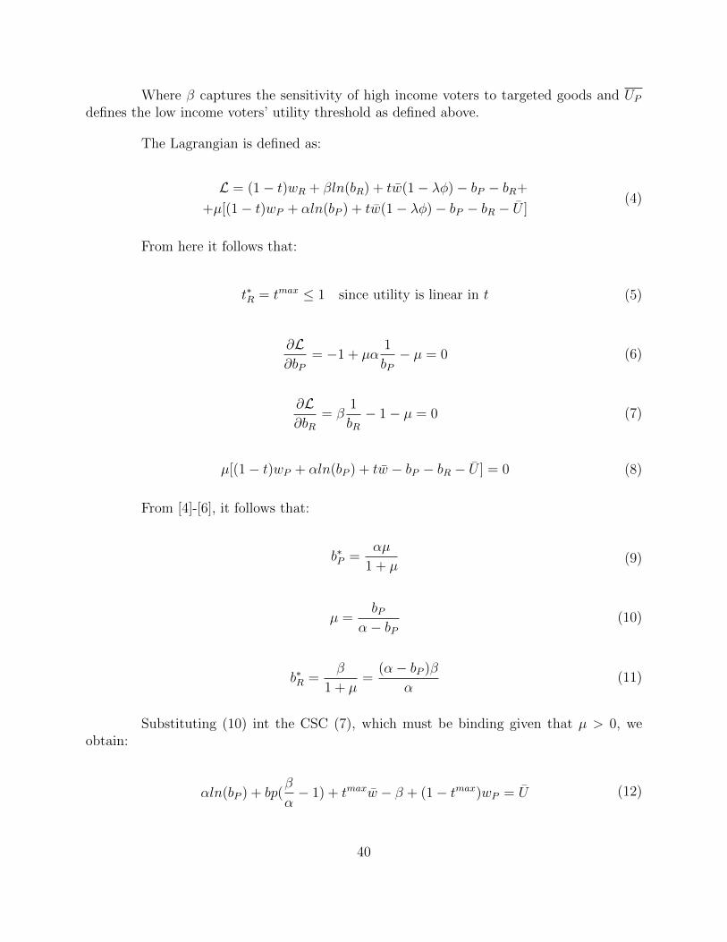
Where β captures the sensitivity of high income voters to targeted goods and UPdefines the low income voters’ utility threshold as defined above.

The Lagrangian is defined as:

L = (1− t)wR + βln(bR) + tw(1− λφ)− bP − bR+

+µ[(1− t)wP + αln(bP ) + tw(1− λφ)− bP − bR − U ](4)

From here it follows that:

t∗R = tmax ≤ 1 since utility is linear in t (5)

∂L∂bP

= −1 + µα1

bP− µ = 0 (6)

∂L∂bR

= β1

bR− 1− µ = 0 (7)

µ[(1− t)wP + αln(bP ) + tw − bP − bR − U ] = 0 (8)

From [4]-[6], it follows that:

b∗P =αµ

1 + µ(9)

µ =bP

α− bP(10)

b∗R =β

1 + µ=

(α− bP )β

α(11)

Substituting (10) int the CSC (7), which must be binding given that µ > 0, weobtain:

αln(bP ) + bp(β

α− 1) + tmaxw − β + (1− tmax)wP = U (12)

40

Inequality and the Elite Choice of Targeted Goods for the Low-Income Voters

From [11] and [12] it follows that

αlnb∗P = β − α + αlnα− tmaxwλ.φ (13)

Which yields

lnb∗P =β

α− 1 + lnα− tmaxwλ.φ

α(14)

From which it follows that

bp∗ = em, where m =

β

α− 1 + ln(α)− τmaxwλφ

α(15)

Which in turn allows us to establish the following comparative statics on the im-pact of inequality on the level of targeted goods towards citizens in the lower half of thedistribution:

1. With respect to the share of income of those above the mean (φ), it follows:

∂ln(bp∗)

∂(φ)=−τmaxwλ

α≤ 0 (16)

Note as well that:∂ln(bp

∗)

∂φ︸︷︷︸≤0

=∂ln(bp

∗)

∂bp︸︷︷︸> 0

b∗p∂φ

From which it follows that:∂b∗p∂φ

< 0

2. With respect to the share of voters below median income (1− δ):

Substituting φ = −wP (1−δ)w

into [13] and differentiating with respect to (1−δ) produces:

∂ln(bp∗)

∂(1− δ)=τmaxwPλ

α≥ 0 (17)

41

Note as well that:∂ln(bp

∗)

∂(1− δ)︸︷︷︸≥0

=∂ln(bp

∗)

∂bp︸︷︷︸> 0

b∗p∂(1− δ)

From which it follows up that:b∗p

∂(1− δ)> 0

Inequality and the Elite Choice of Public Goods

Given the budget constraint and previous results on b∗p, b∗r and tmax we have:

b∗R =(α− bP )β

α

b∗P = em;with m =β

α− 1 + ln(α)− τmaxwλφ

α

Which yields the following budget constraint

tmax[(1− δ)wP + δwR] = em +(α− bP )β

α+ g∗

Rearranging on the basis of previous results, we obtain

g∗ = tmax[(1− δ)wP + δwR]− em − (α− b∗P )β

α

Or developing:

g∗ = tmax[(1− δ)wP + δwR] + (β

α− 1)em − β (18)

Recall that

φ = 1− wP (1− δ)w

Substituting m and subsequently φ into [17] allows us to take the derivative of g∗

42

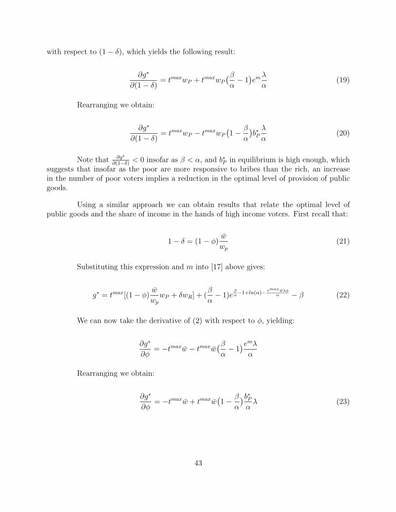
with respect to (1− δ), which yields the following result:

∂g∗

∂(1− δ)= tmaxwP + tmaxwP

(βα− 1)emλ

α(19)

Rearranging we obtain:

∂g∗

∂(1− δ)= tmaxwP − tmaxwP

(1− β

α

)b∗Pλ

α(20)

Note that ∂g∗

∂(1−δ) < 0 insofar as β < α, and b∗P in equilibrium is high enough, whichsuggests that insofar as the poor are more responsive to bribes than the rich, an increasein the number of poor voters implies a reduction in the optimal level of provision of publicgoods.

Using a similar approach we can obtain results that relate the optimal level ofpublic goods and the share of income in the hands of high income voters. First recall that:

1− δ = (1− φ)w

wp(21)

Substituting this expression and m into [17] above gives:

g∗ = tmax[(1− φ)w

wpwP + δwR] + (

β

α− 1)e

βα−1+ln(α)− τmaxwλφ

α − β (22)

We can now take the derivative of (2) with respect to φ, yielding:

∂g∗

∂φ= −tmaxw − tmaxw

(βα− 1)emλα

Rearranging we obtain:

∂g∗

∂φ= −tmaxw + tmaxw

(1− β

α

)b∗Pαλ (23)

43

The Elite’s Choice of Public Goods and the Political Constraint

The results for the elite choice in the presence of the political constraint (U) arethe same as above. In what follows, we solve the maximization problem in the absence ofthe political constraint, and compare the optimal levels of public goods (g∗) under both cir-cumstances (g∗vs.g∗

U). The maximization problem without the political constraint becomes:

maximizet,b,g

Ui(t, b, g) = (1− t)wR + βln(bR) + g

subject to tw = bP + bR + g(24)

maximizet,bR,g

Ui(t, b, g) = (1− t)wR + βln(bR) + tw − bP − bR + g (25)

Solving the problem yields:

• t∗R = tmax ≤ 1

• b∗P = 0

• b∗R = β since ∂Ui∂bR

= β 1bR− 1 = 0

• finally, substituting into the budget constraint and rearranging we obtain g∗ = tmax[(1−δ)wP + δwR]− β

Recall that, by contrast, the level of public goods with the political constraint (g∗U

)

is given by g∗U

= tmax[(1 − δ)wP + δwR] + (βα− 1)bp∗ − β. Comparing the optimal level

of public goods provisions with and without the political constraint produces the followingresult:

g∗ ≶ g∗U

tmaxw − β ≶ tmaxw + (β

α− 1)bp∗ − β

0 ≶ (β

α− 1) bp∗︸︷︷︸

≥0

(26)

This implies that g∗ > g∗U

if β < α and bp∗ > 0.

44

Appendix II: Empirics

Figure 10: Turnout Rates for Municipal Elections in Brazil, 2000 and 2004

02

46

8D

ensi

ty

.6 .7 .8 .9 1

Turnout 2000

02

46

8

.6 .7 .8 .9 1

Turnout 2004

45

Figure 11: Marginal Effect of Inequality on Change in Turnout

-1-.

50

.51

0 1 2 3 4 5 6 0 1 2 3 4 5 6

Not Exposed Exposed

Audited Mismanagement Audited Mismanagement

46

Table 3: Turnout Levels Across Audited Municipalities

DV: Turnout Level in 20003.1 3.2 3.3 3.4

Gini -0.199** -0.189** -0.196** -0.209**(0.091) (0.088) (0.087) (0.086)

Audited Mismanagement -0.023 -0.025 -0.028 -0.030*(0.020) (0.018) (0.019) (0.017)

Gini X Audited Mismanagement 0.053 0.057* 0.061* 0.065**(0.035) (0.033) (0.034) (0.030)

Constant 0.994*** 0.824*** 0.868*** 0.838***(0.051) (0.084) (0.104) (0.107)

Municipality Controls Yes Yes Yes YesInstitutional Controls No Yes Yes YesFederal Transfers and Employment Controls No No Yes YesElectoral Competition Controls No No No YesLottery FEs Yes Yes Yes YesRegional State FEs Yes Yes Yes YesClustered SEs at the Regional Level (26 States) Yes Yes Yes YesObservations 366 366 366 366R-squared 0.543 0.557 0.562 0.576

*** p<0.01, ** p<0.05, * p<0.1

47

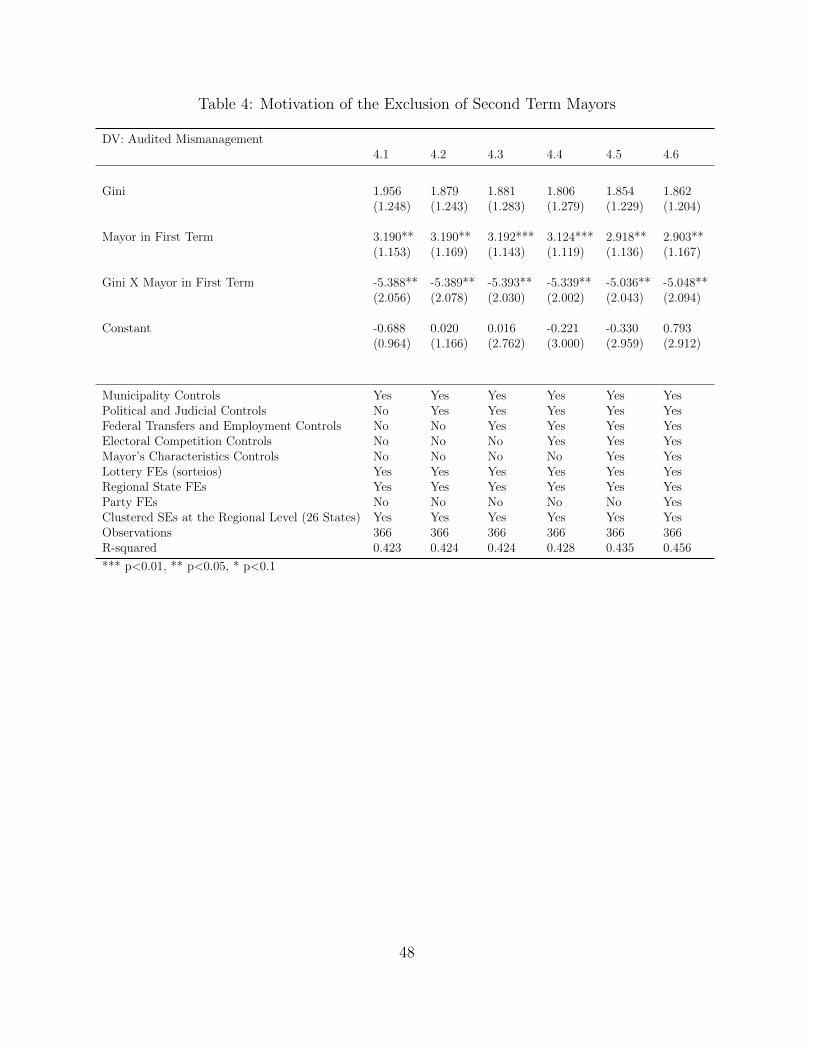
Table 4: Motivation of the Exclusion of Second Term Mayors

DV: Audited Mismanagement4.1 4.2 4.3 4.4 4.5 4.6

Gini 1.956 1.879 1.881 1.806 1.854 1.862(1.248) (1.243) (1.283) (1.279) (1.229) (1.204)

Mayor in First Term 3.190** 3.190** 3.192*** 3.124*** 2.918** 2.903**(1.153) (1.169) (1.143) (1.119) (1.136) (1.167)

Gini X Mayor in First Term -5.388** -5.389** -5.393** -5.339** -5.036** -5.048**(2.056) (2.078) (2.030) (2.002) (2.043) (2.094)

Constant -0.688 0.020 0.016 -0.221 -0.330 0.793(0.964) (1.166) (2.762) (3.000) (2.959) (2.912)

Municipality Controls Yes Yes Yes Yes Yes YesPolitical and Judicial Controls No Yes Yes Yes Yes YesFederal Transfers and Employment Controls No No Yes Yes Yes YesElectoral Competition Controls No No No Yes Yes YesMayor’s Characteristics Controls No No No No Yes YesLottery FEs (sorteios) Yes Yes Yes Yes Yes YesRegional State FEs Yes Yes Yes Yes Yes YesParty FEs No No No No No YesClustered SEs at the Regional Level (26 States) Yes Yes Yes Yes Yes YesObservations 366 366 366 366 366 366R-squared 0.423 0.424 0.424 0.428 0.435 0.456

*** p<0.01, ** p<0.05, * p<0.1

48

Table 5: Balance Tables for the Control (Not-Exposed) and Treatment (Exposed) Groups

Not Exposed MunicipalitiesVariable Mean Std. Dev. N

mismanagement 1.789 1.174 37gini ipea 0.578 0.065 68lpib02 -0.927 0.872 68lpop 9.82 1.01 68purb 0.629 0.226 68p secundario 0.246 0.106 68mun novo 0.191 0.396 68area 2.129 3.435 68comarca 0.603 0.493 68vereador eleit 11.695 8.723 68lrec trans 16.006 0.947 68lfunc ativ 6.287 0.929 68ENLP2000 4.735 1.921 68winmargin 0.151 0.142 68samepartygov98 0.206 0.407 68pref masc 0.971 0.17 68pref idade tse 46.985 9.426 68exp prefeito 0.279 0.452 68pref escola 6.279 1.752 68p cad pref 0.251 0.148 68vereador9600 0.074 0.263 68op 01 04 0.015 0.121 68ratioaptos 1.072 0.144 68media2 0.853 0.357 68

Exposed MunicipalitiesVariable Mean Std. Dev. N

mismanagement 1.624 1.198 166gini ipea 0.571 0.063 199lpib02 -1.054 0.758 199lpop 9.552 0.964 199purb 0.617 0.225 199p secundario 0.246 0.097 199mun novo 0.221 0.416 199area 2.263 7.256 199comarca 0.553 0.498 199vereador eleit 15.051 11.775 199lrec trans 15.797 0.809 199lfunc ativ 6.060 0.817 199ENLP2000 4.492 1.801 199winmargin 0.143 0.161 199samepartygov98 0.241 0.429 199pref masc 0.940 0.239 199pref idade tse 48.266 9.113 199exp prefeito 0.312 0.464 199pref escola 6.005 1.874 199p cad pref 0.276 0.142 199vereador9600 0.111 0.314 199op 01 04 0.03 0.171 199ratioaptos 1.104 0.141 198media2 0.829 0.377 199

49

Table 6: The Mechanism: Local Media Presence versus No Local Media

DV: Turnout Change 2004-2000 No Local Media Local Media6.1 6.2 6.3 6.4 6.5 6.6

Gini -1.520 -2.108* -3.089** -0.181 -0.275 -0.291(0.905) (1.117) (1.343) (0.157) (0.168) (0.175)

Mismanagement -0.219 -0.351 -0.536** -0.087** -0.108*** -0.112**(0.175) (0.229) (0.245) (0.038) (0.038) (0.044)

Gini X Mismanagement 0.395 0.619 0.908** 0.149** 0.183** 0.188**(0.298) (0.384) (0.412) (0.070) (0.067) (0.078)

Exposed -0.510 -1.020 -1.440 -0.203* -0.285** -0.299**

(0.592) (0.702) (0.870) (0.108) (0.112) (0.121)Exposed X Gini 1.019 1.929 2.577 0.314 0.450** 0.468**

(1.031) (1.186) (1.508) (0.190) (0.194) (0.202)Exposed X Mismanagement 0.187 0.403* 0.542* 0.133** 0.162*** 0.170***

(0.206) (0.220) (0.282) (0.054) (0.051) (0.058)Exposed X Gini X Mismanagement -0.389 -0.760* -0.967* -0.246** -0.295*** -0.304***

(0.354) (0.357) (0.485) (0.101) (0.096) (0.107)

Constant 2.014 2.387 3.264 0.251 0.320 0.322(1.289) (1.438) (1.953) (0.191) (0.194) (0.197)

Municipality & Institutional Controls Yes Yes Yes Yes Yes YesElectoral Competition Controls No Yes Yes No Yes YesMayor’s Characteristics Controls No No Yes No No YesLottery FEs Yes Yes Yes Yes Yes YesClustered SEs at the Regional Level (26 States) Yes Yes Yes Yes Yes YesObservations 40 40 40 163 163 163R-squared 0.751 0.831 0.916 0.617 0.628 0.646

*** p<0.01, ** p<0.05, * p<0.1

50

Table 7: The Mechanism: Strong Opposition versus Weak Opposition

Turnout Change 2004-2000 Strong Opposition Weak Opposition7.1 7.2 7.3 7.4 7.5 7.6

Gini -0.070 -0.105 -0.201 -0.845 -1.333** -1.285*(0.137) (0.151) (0.223) (0.561) (0.574) (0.714)

Mismanagement 0.015 0.006 -0.016 -0.290** -0.360*** -0.339**(0.043) (0.047) (0.059) (0.126) (0.122) (0.135)

Gini X Mismanagement -0.021 -0.005 0.028 0.527** 0.644*** 0.610**(0.065) (0.073) (0.093) (0.217) (0.206) (0.228)

Exposed -0.083 -0.103 -0.147 -0.545* -0.758** -0.740*(0.097) (0.118) (0.131) (0.300) (0.275) (0.359)

Exposed X Gini 0.142 0.179 0.257 1.063* 1.473** 1.425*(0.156) (0.192) (0.213) (0.575) (0.536) (0.712)

Exposed X Mismanagement 0.044 0.050 0.073 0.301** 0.370*** 0.343**(0.061) (0.062) (0.066) (0.143) (0.118) (0.139)

Exposed X Gni X Mismanagement -0.111 -0.120 -0.155 -0.552** -0.670*** -0.624**(0.099) (0.101) (0.108) (0.244) (0.197) (0.229)

Constant 0.238 0.247 0.279 0.389 0.967** 0.895(0.155) (0.164) (0.164) (0.363) (0.407) (0.645)

Municipality & Institutional Controls Yes Yes Yes Yes Yes YesElectoral Competition Controls No Yes Yes No Yes YesMayor’s Characteristics Controls No No Yes No No YesLottery FEs Yes Yes Yes Yes Yes YesClustered SEs at the Regional Level (26 States) Yes Yes Yes Yes Yes YesObservations 140 140 140 63 63 63R-squared 0.495 0.500 0.530 0.790 0.820 0.827

*** p<0.01, ** p<0.05, * p<0.1

51

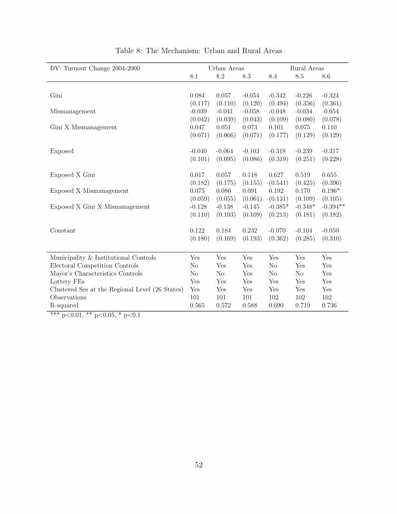
Table 8: The Mechanism: Urban and Rural Areas

DV: Turnout Change 2004-2000 Urban Areas Rural Areas8.1 8.2 8.3 8.4 8.5 8.6

Gini 0.084 0.057 -0.054 -0.342 -0.226 -0.324(0.117) (0.110) (0.120) (0.494) (0.356) (0.361)

Mismanagement -0.039 -0.041 -0.058 -0.048 -0.034 -0.054(0.042) (0.039) (0.043) (0.109) (0.080) (0.078)

Gini X Mismanagement 0.047 0.051 0.073 0.101 0.075 0.110(0.071) (0.066) (0.071) (0.177) (0.129) (0.129)

Exposed -0.040 -0.064 -0.103 -0.318 -0.239 -0.317(0.101) (0.095) (0.086) (0.319) (0.251) (0.228)

Exposed X Gini 0.017 0.057 0.118 0.627 0.519 0.655(0.182) (0.175) (0.155) (0.541) (0.425) (0.396)

Exposed X Mismanagement 0.075 0.080 0.091 0.192 0.170 0.196*(0.059) (0.055) (0.061) (0.131) (0.109) (0.105)

Exposed X Gini X Mismanagement -0.128 -0.138 -0.145 -0.385* -0.348* -0.394**(0.110) (0.103) (0.109) (0.213) (0.181) (0.182)

Constant 0.122 0.184 0.232 -0.070 -0.104 -0.050(0.180) (0.169) (0.193) (0.362) (0.285) (0.310)

Municipality & Institutional Controls Yes Yes Yes Yes Yes YesElectoral Competition Controls No Yes Yes No Yes YesMayor’s Characteristics Controls No No Yes No No YesLottery FEs Yes Yes Yes Yes Yes YesClustered Ses at the Regional Level (26 States) Yes Yes Yes Yes Yes YesObservations 101 101 101 102 102 102R-squared 0.565 0.572 0.588 0.690 0.719 0.736

*** p<0.01, ** p<0.05, * p<0.1

52

Table 9: Cross Section: Second Stage Regression, Programmatism Measure

Second Stage Weighted Regressions Low-Income Voters Turnout βLQ,j Turnout Inequality βdiff,j9.1 9.2 9.3 9.4 9.5 9.6

Gini Net 0.299** 0.337*** 0.312* -0.351*** -0.330*** -0.289*(0.114) (0.092) (0.153) (0.110) (0.100) (0.166)

Programmatism 0.354* 0.327** 0.201 -0.314** -0.309** -0.179(0.173) (0.122) (0.169) (0.126) (0.124) (0.170)

Gini Net X Programmatism -0.423** -0.413*** -0.329* 0.414*** 0.403*** 0.310(0.160) (0.117) (0.181) (0.122) (0.120) (0.182)

High Income Voters Turnout (βHQ,j) 0.607*** 0.548*** 0.297** 0.320*(0.078) (0.094) (0.117) (0.161)

Constant -0.043 -0.087 -0.120 0.119 0.103 0.158(0.113) (0.114) (0.184) (0.130) (0.127) (0.210)

Controls Yes Yes Yes Yes Yes YesBorjas Weighting Yes Yes Yes Yes Yes YesClustered Std Errors at the Country Level Yes Yes Yes Yes Yes YesHigh Quality Gini Dataset (Solt 4.0) Yes Yes Yes Yes Yes YesClientelism Data Time Trend Correction No No Yes No No YesCSES Waves 1,2&3 1,2&3 1,2&3 1,2&3 1,2&3 1,2&3Countries 30 30 25 30 30 25Observations (Country-year) 75 75 47 75 75 47R-squared 0.318 0.607 0.592 0.683 0.736 0.708Controls Include: lnGDPpc, Redistribution, Compulsory Voting, PR, lnPOP, Polity2, Mortality Rate, GDP Growth, Globalization Index

*** p<0.01, ** p<0.05, * p<0.1

53

Figure 12: Marginal Effect of Inequality on Low Income Voters Turnout

-.4

-.2

0.2

.4

-1.4 -1 -.5 0 .5 1 1.5 2 2.5

Clientelism Measure (standardized)

-.4

-.2

0.2

.4

-1.5 -1 -.5 0 .5 1 1.5 2 2.5

Programmatism Measure (standardized)

54

Economic and Political Inequality: The Role of Political ... · Economic and Political Inequality:...

Documents

Transcript of Economic and Political Inequality: The Role of Political ... · Economic and Political Inequality:...