Economic analysis with Stata 6.0/7 - fm · PDF fileEconomic analysis with Stata 6.0/7.0 ......

January 25, 2001

Economic analysiswith Stata 6.0/7.0

Christopher F BaumDepartment of Economics andFaculty Microcomputer Resource CenterBoston College

January 25, 2001

Introduction� Stata: a statistical programming language with

particular strengths in data manipulation and theanalysis of cross-sectional and panel data

� Most similar in capabilities to SAS, but muchsimpler, more concisely documented, and far lessexpensive

� More programmable and cross-platform than SPSS� Narrower features for time series analysis than

RATS, but rapidly adding these capabilities

January 25, 2001

Portability

� One of the most portable, cross-platform-capablelanguages available for econometric analysis

� Versions available for Mac OS, Windows95/98/NT/2000, flavors of UNIX and Linux

� Binary datafiles transportable without translationacross all platforms

� Stata programs run without modification across allplatforms

� Full versions available at low cost to academics

January 25, 2001

Extensibility

� Much of Stata is written in its own language, andmay be studied and extended

� Stata procedures (.ado files), when placed on theADOPATH, are automatically available to your copyof Stata as a new command

� Bimonthly issues of the Stata Technical Bulletin(STB) contain new procedures in a peer-reviewed,tested context; these are linked to online help andfreely available for download over the Web

January 25, 2001

User Support

� Stata itself is Internet-upgradable, as are user-contributed components

� Users and StataCorp participate vigorously inStataList, a moderated Listserv mailing list,responding rapidly to users enquiries

� All StataList ado-files are posted to the BostonCollege Statistical Software Components Archive(SSC-IDEAS), from which they may be freelydownloaded. The archive is searchable from withinStata, and items are Internet-installable.

January 25, 2001

On-line help

� Full help for all Stata commands is available fromthe help’ command in a man page format

� ‘search topic name’ will locate instances ofthat string anywhere within the help system

� A series of on-line tutorials exhibits the majorfeatures of the program

� The four-volume hardcopy Reference Manual andone-volume User s Guide provide fulldocumentation and present the underlying formulasand references

January 25, 2001

Dataset concepts

� Stata s speed results from its holding the entiredataset in memory

� Only one dataset may be used at a time;sophisticated techniques for merging allow thecombining of several files into one

� Binary datasets created by Stata usually are giventhe filetype .dta on all platforms

� Access to binary datasets is much faster thanaccess to text files

January 25, 2001

Memory allocation

� Stata starts with a default memory allocation whichmay not be sufficient for working with a largedataset

� UNIX Stata may be invoked with the -kNNNN switch(stata -k50000 would allocate 50 Mb ofmemory) or the command ‘set mem 50m’ maybe given within the program. No more than 130 Mbis available under AIX; more under Solaris.

� Macintosh Stata memory allocation may beadjusted via the Get Info box on the File menu.

January 25, 2001

Command-linemode

� Stata in its standard form is a command-lineprogram on all platforms, with a dot prompt

� The StataQuest additions (freely downloadablefrom www.stata.com) turn any desktop copy ofStata into a limited-feature, menu-driven programsuitable for a beginning statistics course, in whichthe student may point and click to select allavailable features of the program

� A shell escape (!) may be used to access UNIXduring a Stata session

January 25, 2001

‘Batch’ mode

� Any version of Stata may run a program withoutuser intervention.

� In UNIX Stata, run the program myjob.do withstata -b do myjobwhich will place the output in myjob.log.

� To run this as a true batch job, give the UNIXcommand batch first, type the Stata commandline, and use CTRL-D to submit the batch job.

� In Mac Stata, launch the do-file to execute theprogram within.

January 25, 2001

Desktop Stata

� In a desktop version of Stata, an additional windowcontains a log of all commands given. You mayselect any command to bring it into the commandwindow, edit it, and execute it without retyping. Asecond window lists all the variables in the currentdataset with their variable labels.

� Logging of commands and results to a text file maybe started and stopped during the session

� Graphs may be generated and viewed; in the UNIXcommand-line version, they may not be viewed

January 25, 2001

Case sensitivity

� Like UNIX, Stata is case-sensitive. It expects thatcommands will be given in lower case. Thevariables price, PRICE, and Price are differentvariables. To avoid problems, stick with lower casethroughout.

� UNIX file names and directory names must begiven in the same case in which they appear in theoperating system.

January 25, 2001

Getting your data in

� Comma-delimited (CSV) or tab-delimited data mayusually be read very easily with the insheetcommand (which does not read spreadsheets!)

� insheet using filename’ will expect thatyour data are in the ASCII text filefilename.raw’. If the filetype is not .raw, it mustbe specified. You need not specify comma- ortab-delimiting.

� If the first line of the file contains variable names,they will be automatically used within the program.

January 25, 2001


� Variables may contain either numeric or string data.Functions exist to create numeric codes from a setof string values, or to convert string values withpurely numeric contents to their numericequivalents.

� The insheet command cannot read space-delimited data (even if it is purely numeric). Space-delimited data may be read with the infile or infixcommands.

January 25, 2001


� A free-format text file with space- (or tab- orcomma-) delimited numeric data may be read withinfile; i.e.infile price mpg displ using auto’will read those three variables from the ASCII fileauto.raw. The number of observations will bedetermined from the available data.

� The common missing-data indicator . (period)may be used to flag values as missing. This easesimportation of text files written by SAS.

January 25, 2001


� Infile may also be used with fixed-format data,including data containing undelimited stringvariables, by creating a dictionary file (.dct) whichdescribes the format of each variable and specifieswhere the data are to be found.

� If data are packed tightly, with no delimiters, adictionary must be used to define the variableslocations.

� The _column() directive allows contents of a datarecord to be retrieved selectively.

January 25, 2001


� The byvariable() option to infile allows avariable-wise data set to be read; the number of

observations must be specified as the value of theoption. This is often useful when working with time-series data which may have been retrieved variableby variable, rather than in a columnar format.

� The infix’ command presents a syntax similar tothat used by SAS for the definition of variablestypes and locations in a fixed-format ASCII dataset.

January 25, 2001


� A logical condition may be applied on the infile orinfix commands to read only those records forwhich certain conditions are satisfied; i.e. infix using employee if sex==‘M’will read only male employees records from theexternal file, while infile price mpg using auto in 1/20would read only the first 20 observations of theexternal file.

January 25, 2001


� If your data are already in the internal format ofSAS, SPSS, Excel, GAUSS, Lotus, or several otherprograms, you should use Stat/Transfer: the SwissArmy knife of data converters. It is available forWindows and on fmrisc.bc.edu and econ.bc.edu(stattransfer).

� Use of Stat/Transfer will preserve variable labels,value labels, and other aspects of the data thatmight be lost if the data were converted to a pureASCII file.

January 25, 2001

Working with storeddata

� If you have saved your data in Stata binary format(in a .dta file), you employ the use filenamecommand to make it the currently active datafile (orlaunch the file on a desktop version of Stata).

� If you want to merge files, both must be in .dtaformat, and you must use sort to arrange eachdataset according to the order of the mergevariable(s). Stata can handle one-to-one, one-to-many, and many-to-one merges.

January 25, 2001

Language syntax

� Stata commands follow a common syntax:[by varlist:] command [varlist] [=exp]

[if exp] [in range] [weight] [,options]

where [ ] indicate optional qualifiers.� ˚command is a Stata command� varlist is a list of variable names� exp is an algebraic expression� options denotes a list of options

January 25, 2001

Language syntax

� varlist may be optional; if none is given, _all isassumed. Commands that alter or destroy datarequire an explicit varlist.

� For instance, the command ‘summarize’ withoutadditional arguments gives descriptive statistics forall currently defined variables.

� The command ‘drop price mpg’ will removethose variables; ‘drop _all’ is required toremove all currently defined variables.

January 25, 2001

Language syntax

� The by varlist: prefix may be used with manycommands to instruct Stata to repeat the commandfor each value of the varlist (which will sensibly becomprised of integer-valued numeric variablesand/or string variables). This is very powerful; e.g.by race sex : summ incomewill generate descriptive statistics for eachcombination of the two categorical variables.

� The dataset must be sorted by the variables ofthe varlist prior to use of the by varlist: prefix.

January 25, 2001

Language syntax

� The if exp qualifier restricts the scope of thecommand to that of the logical expression. This canbe used to evaluate a subset, e.g., to run aregression on only black males, or to construct adummy variable conditional on certain features ofthe data.

� Note that logical expressions make use of == forequality, & for the AND operator, | for the ORoperator, != for the NOT operator. The wordsAND, OR, NOT are not used in Stata syntax.

January 25, 2001

Language syntax

� The in range qualifier restricts the scope of thecommand to a specific observation range:1/10 denotes observations 1 through 10;-5/-1 denotes the last five observations.

� This qualifier may be used to examine a fewobservations, or to pick out the top n observationsafter sorting the data.

� The in range qualifier may not be used inconjunction with the by varlist: prefix.

January 25, 2001

Language syntax

� The =exp expression is most often used in creatingnew variables, via the generate (gen) command.

� If an existing variable is to be modified, the replacecommand must be used, and replace cannot beabbreviated.

� Creating a dummy variable is best done with alogical expression:gen down = (gdpgro < 0)

� The egen command provides an additional anduser-expandable set of functions

January 25, 2001

Language syntax

� Weights may also be applied in the context of manycommands. Several different weighting schemes(analytic weights, frequency weights, samplingweights, importance weights) are available.

� Weighting is most commonly applied when workingwith survey data or cross-sectional data thatrepresent groupings of microdata.

January 25, 2001

Language syntax

� Most commands take command-specific options.All options appear at the end of the command aftera single comma.

� Options generally have default values. Many aretoggles, with values of opt or noopt, such assummarize price mpg, detailwhich will generate extended descriptive statistics.The default choice is nodetail, which thus neednot be given.

� Some options take numeric or string arguments.

January 25, 2001

File handling

� File extensions usually employed (but not required)include:

� .ado automatic do-file (procedure)� .dct data dictionary� .do do-file (user program)� .dta Stata binary dataset� .gph graph output file (binary)� .log log file (text)� .raw ASCII data file

January 25, 2001

File handling

� If you employ the common file extensions, youneed not use them explicitly in Stata commands;

� infile using mydatpresumes mydat.raw

� save myfile, replacepresumes myfile.dta

� do myprogpresumes myprog.do

� Exception: ado-files must have filetype ado.

January 25, 2001

File handling

� For ease of use, Macintosh Stata users shouldemploy menu commands such as File->Open andFile->Filename to access files on the hard disk.

� The default Macintosh hard disk name,Macintosh HD, is problematic. Give the hard disk aname that does not contain embedded spaces.

� All desktop users should make use of an adodirectory to store ado-files that are not distributedby Stata or STB. The adopath command specifiesthe expected location of this directory.

January 25, 2001

Data characteristics

� Stata stores data in three integer datatypes: byte,int, long and two floating point formats: floatand double. There is also a date datatype.

� Stata handles string data, with varying-lengthstrings (max 80 bytes), and the missing string .

� To use categorical variables in statistical routines,the encode command may be used to transform,e.g., sex={ male , female } viaencode sex, gen(gender)where gender will now be a dummy variable.

January 25, 2001


� If a string variable ‘myvar’ contains the characterrepresentation of a number, it may be converted toa numeric variable viagen newvar = real(myvar)or via the more powerful conv2num’ command(an STB addition).

� A numeric variable may be converted to itscharacter string equivalent viagen str10 svar = string(newvar)which should reproduce myvar.

January 25, 2001


� Each variable may have its own default displayformat. This does not govern the contents of thevariable, but affects how it is displayed. Forinstance, %9.2f would generate dollars andcents , like the FORTRAN format element F9.2.The commandformat varname formatspec e.g.format gdp %9.1fwill store that display format with the variable in theStata dataset.

January 25, 2001


� Each variable may have its own variable label: a31-character string which describes the variable,associated with the variable vialabel variable varname “text”.

� Variable labels, where defined, will be used toidentify the variable in printed output, spacepermitting.

January 25, 2001


� Value labels associate numeric values withcharacter strings; if a mapping is defined aslabel define sexlbl 0 “male” 1 “female”then a numeric (dummy) variable sex may be givenvalue labels vialabel values sex sexlbl

� If value labels are present, they will appear onprinted output rather than their numericequivalents.

January 25, 2001


� Value labels may be generated when reading dataif string variables take on specific values:infile empno sex:sexlbl salary using

empfile, automaticThe sexlbl qualifier indicates, in conjunction withthe automatic option, that a set of value labelsare to be defined as ‘sexlbl’ from the discretecharacter values read from the sex’ variable. Inthis case sex becomes a numeric variable, withassociated value labels as defined by sexlbl.

January 25, 2001

Functions

� Functions appear in expressions in the generate,replace, and egen statements in which variablesare created.

� Functions also appear in the if exp qualifiers ofmany commands in which logical expressions areused to constrain the command.

� +, -, *, / have their usual meaning; ^ denotesexponentiation.

� + is also used as the concatenation operator forstrings.

January 25, 2001

Functions

� Relational operators include >, >=, <, <=, == forequality, and ~= for inequality. != may also beused for inequality.

� The most common error in constructing if expqualifiers is the use of = where == is appropriate.

� Logical operators include & for AND, | for OR, and~ for NOT. The words are not used. There is noexclusive OR (XOR) operator.

January 25, 2001

Functions

� Mathematical functions include the usual:abs(), exp(), ln(), log() [both referring tonatural log], mod(x,y), sqrt(), and thetrigonometric functions (with arguments in radians).

� The lnfact(n) function is the natural log of n!.� The mod(x,y) is x modulo y.� Statistical functions include those for binomial, χ2,

F, gamma, beta, normal, t, and uniform distributionsand their inverses, as well as cumulativedistribution functions for many distributions.

January 25, 2001

Functions

� Date functions allow manipulation of the portions ofa date variable, and the calculation of elapsed time.

� String functions permit detection of a character orsubstring within a string, extraction of first, last, orspecified substring, trimming, and case conversion.

� Special functions include coding (creating bracketsof a numeric variable), integer truncation/floatingpoint conversion, min, max, round, sign, and sum(the running sum of a variable).

January 25, 2001

Functions

� The egen command (extensions to generate)provides a number of special functions, includingthose which operate on a set of variables: forinstance, row sums (rsum()), row means(rmean()), row standard deviations (rsd()). Theegen command also computes percentiles,medians, and ranks.

� The egen command may be user-extended, as allegen functions are implemented as _gfunc.adofiles.

January 25, 2001

Estimationcommands

� All estimation commands share the same syntax.� Multiple equation estimation commands use an

eqlist rather than a varlist, where equations aredefined prior to estimation via the eq command.

� Estimation commands display confidence intervalsfor the coefficients; the level() option controlsthe width of the intervals.

� The variance-covariance matrix of the estimatorsmay be retrieved with the vce command.

January 25, 2001

Estimationcommands

� Predicted values and residuals may be obtainedafter estimation with the predict command. Thefit command may be used as an alternative to‘regress’ to generate a number of influencemeasures.

� After estimation, coefficients and standard errorsmay be used in expressions; _b[income] is theestimated coefficient on income in the lastregression, while _se[income] refers to itsestimated standard error.

January 25, 2001

Estimationcommands

� Linear hypothesis (Wald) tests on the estimatedparameters may be performed with the testcommand. The ‘nltest’ command providesWald tests of nonlinear hypotheses, while the‘lrtest’ command performs likelihood ratiotests.

� Robust (Huber/White) sandwich estimates of thevariance-covariance matrix are available for manyestimation commands by specifying the robustoption.

January 25, 2001

Estimationcommands

� OLS estimates may be generated by the regresscommand, where the varlist contains the dependentvariable followed by independent variables. Aconstant term is supplied by default; noconssuppresses the constant term.

� Following regression, predict yhat will generatethe (in-sample) predicted values as variable yhat.Out-of-sample predictions may be generated byusing an if exp or an in range qualifier toselect observations not used in the estimation.

January 25, 2001

Estimationcommands

� The predict command can also be used togenerate estimated residuals (in- and out-of-sample), as well as standardized residuals, thestandard error of the prediction, and the standarderror of forecast.

� predict may be used following many estimationcommands—not merely OLS regression. Forinstance, it may be used to predict estimatedprobabilities following estimation of a binomial logitor probit model.

January 25, 2001

Estimationcommands

� Basic statistical commands:� summarize: descriptive statistics� table, tabsum, tabulate: tables of summary

statistics and frequencies� anova: analysis of variance and covariance� oneway: one-way analysis of variance� correlate: correlations, covariances� ttest: mean comparison tests

January 25, 2001

Estimationcommands

� Regression commands:� regress: OLS, IV, 2SLS regression� predict, fit: predictions, fit diagnostics� cnreg, tobit: censored-normal, Tobit models� nl: nonlinear least squares� xtreg, xtgls, xtgee: panel data models� glm: general linear models� heckman: Heckman s selection model

January 25, 2001

. ttest mpg,by(foreign)

Two-sample t test with equal variances Domestic: Number of obs = 52 Foreign: Number of obs = 22

------------------------------------------------------------------------------Variable | Mean Std. Err. t P>|t| [95% Conf. Interval]---------+--------------------------------------------------------------------Domestic | 19.82692 .657777 30.1423 0.0000 18.50638 21.14747 Foreign | 24.77273 1.40951 17.5754 0.0000 21.84149 27.70396---------+-------------------------------------------------------------------- diff | -4.945804 1.362162 -3.63085 0.0005 -7.661225 -2.230384------------------------------------------------------------------------------Degrees of freedom: 72

Ho: mean(Domestic) - mean(Foreign) = diff = 0

Ha: diff < 0 Ha: diff ~= 0 Ha: diff > 0 t = -3.6308 t = -3.6308 t = -3.6308 P < t = 0.0003 P > |t| = 0.0005 P > t = 0.9997

.

January 25, 2001

. regress price mpg hdroom displ foreign

Source | SS df MS Number of obs = 74---------+------------------------------ F( 4, 69) = 16.36 Model | 309109608 4 77277401.9 Prob > F = 0.0000Residual | 325955789 69 4723996.94 R-squared = 0.4867---------+------------------------------ Adj R-squared = 0.4570 Total | 635065396 73 8699525.97 Root MSE = 2173.5

------------------------------------------------------------------------------ price | Coef. Std. Err. t P>|t| [95% Conf. Interval]---------+-------------------------------------------------------------------- mpg | -113.1064 62.72059 -1.803 0.076 -238.2305 12.01778 hdroom | -613.7925 344.3983 -1.782 0.079 -1300.848 73.2633 displ | 24.4052 4.699919 5.193 0.000 15.02911 33.78128 foreign | 3529.337 702.0066 5.027 0.000 2128.872 4929.801 _cons | 4547.006 2323.137 1.957 0.054 -87.52626 9181.537------------------------------------------------------------------------------

January 25, 2001

. regress price mpg hdroom displ if foreign==0

Source | SS df MS Number of obs = 52---------+------------------------------ F( 3, 48) = 16.06 Model | 245079940 3 81693313.3 Prob > F = 0.0000Residual | 244114861 48 5085726.27 R-squared = 0.5010---------+------------------------------ Adj R-squared = 0.4698 Total | 489194801 51 9592054.92 Root MSE = 2255.2

------------------------------------------------------------------------------ price | Coef. Std. Err. t P>|t| [95% Conf. Interval]---------+-------------------------------------------------------------------- mpg | -35.37898 104.8593 -0.337 0.737 -246.2128 175.4548 hdroom | -645.0291 397.923 -1.621 0.112 -1445.107 155.0487 displ | 26.44172 5.597903 4.724 0.000 15.18638 37.69706 _cons | 2628.467 3558.628 0.739 0.464 -4526.634 9783.567------------------------------------------------------------------------------

January 25, 2001

Estimationcommands

� A sampling of other estimation commands:� sureg, reg3: Zellner s SUR/3SLS� qreg: quantile (including median) regression� logit, probit: binomial logit/probit� ologit, oprobit: ordered logit/probit� mlogit: multinomial logit� survival analysis models� bstrap: bootstrap sampling� ml: maximum likelihood estimation

January 25, 2001

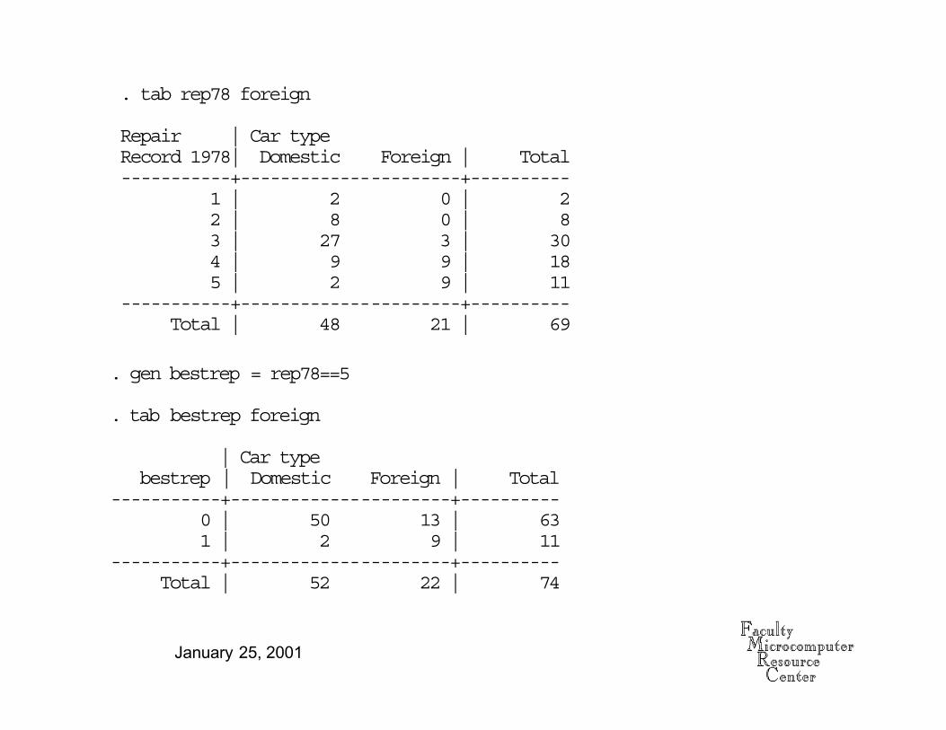
. gen bestrep = rep78==5

. tab bestrep foreign

| Car type bestrep | Domestic Foreign | Total-----------+----------------------+---------- 0 | 50 13 | 63 1 | 2 9 | 11-----------+----------------------+---------- Total | 52 22 | 74

. tab rep78 foreign

Repair | Car typeRecord 1978| Domestic Foreign | Total-----------+----------------------+---------- 1 | 2 0 | 2 2 | 8 0 | 8 3 | 27 3 | 30 4 | 9 9 | 18 5 | 2 9 | 11 -----------+----------------------+---------- Total | 48 21 | 69

January 25, 2001

. logit bestrep price mpg foreign

Iteration 0: Log Likelihood =-31.106481Iteration 1: Log Likelihood =-22.171647Iteration 2: Log Likelihood =-20.124399Iteration 3: Log Likelihood =-20.031529Iteration 4: Log Likelihood = -20.03006Iteration 5: Log Likelihood =-20.030059

Logit Estimates Number of obs = 74 chi2(3) = 22.15 Prob > chi2 = 0.0001Log Likelihood = -20.030059 Pseudo R2 = 0.3561

------------------------------------------------------------------------------ bestrep | Coef. Std. Err. z P>|z| [95% Conf. Interval]---------+-------------------------------------------------------------------- price | .0001738 .0001754 0.991 0.322 -.00017 .0005175 mpg | .2077759 .0921829 2.254 0.024 .0271006 .3884511 foreign | 2.155065 .8933987 2.412 0.016 .4040353 3.906094 _cons | -8.792186 3.065257 -2.868 0.004 -14.79998 -2.784393------------------------------------------------------------------------------

January 25, 2001

. ologit rep78 price mpg foreign

Iteration 0: Log Likelihood =-93.692061Iteration 1: Log Likelihood =-78.391154Iteration 2: Log Likelihood =-77.587155Iteration 3: Log Likelihood =-77.567314Iteration 4: Log Likelihood =-77.567278

Ordered Logit Estimates Number of obs = 69 chi2(3) = 32.25 Prob > chi2 = 0.0000Log Likelihood = -77.567278 Pseudo R2 = 0.1721

------------------------------------------------------------------------------ rep78 | Coef. Std. Err. z P>|z| [95% Conf. Interval]---------+-------------------------------------------------------------------- price | .0000931 .0000921 1.011 0.312 -.0000874 .0002735 mpg | .0983342 .0588177 1.672 0.095 -.0169465 .2136148 foreign | 2.455968 .6850463 3.585 0.000 1.113301 3.798634---------+-------------------------------------------------------------------- _cut1 | -.7119252 1.656026 (Ancillary parameters) _cut2 | 1.090715 1.540291 _cut3 | 3.719323 1.580065 _cut4 | 5.80092 1.688265 ------------------------------------------------------------------------------

January 25, 2001

Timeseries

� In Versions 6 and 7, Stata has added a broad set oftimeseries capabilities.

� The tsset command allows specification of thetimeseries calendar associated with a dataset.Dates may be displayed in many formats. Seetsmktim on SSC-IDEAS to set up a timeseriesdataset.

� Annual, half yearly, quarterly, monthly, weekly, anddaily frequencies are supported.

January 25, 2001

Timeseries

� Functions tin(d1,d2) and twithin(d1,d2)permit specification of date ranges fortransformations and analysis.

� Lagged (and led) values or differences oftimeseries data may be specified on the fly : e.g.regress gdp L(1/4).gdpregress D.gdp L.gdpwill run an AR(4) model and the Dickey-Fullerregression, respectively.

January 25, 2001

Timeseries

� Timeseries estimation commands include arch,arima, dfuller / pperron, corrgram / xcorr,and wntestq (Q-test). The Arellano-Bond dynamicpanel data estimators are available in Stata 7.

� Timeseries commands available from SSC-IDEASinclude arimafit, durbinh, bgtest (Breusch-Godfrey test for autocorrelation), dfgls (improvedDickey-Fuller test), kpss (unit root test), and anumber of long memory estimators.

January 25, 2001

Panel data

� Stata is perhaps the most versatile statisticspackage for the handling of panel (longitudinal)data, balanced or unbalanced. The commands iisor tis define the unit and time identifier variables;tsset may also be used to define a panel.

� Transformations on panel data understand thenature of the data, so that lagged values (L.var)and differences (D.var) will not extend into theprevious unit s data.

January 25, 2001

Panel data

� The xt commands allow you to describe,summarize, and estimate models on panel data.xtreg, fe estimates fixed effects models;xtreg, re estimates random effects models.More complex models may be implemented withthe xtregar, xtgls and xtivreg commands.

� It is very easy to calculate summary statistics foreither dimension of a panel, or generate a newdataset containing e.g. time-averaged individualobservations. See collapse.

January 25, 2001

Graphics

� Stata contains extensive graphics capabilities forthe generation of bar, box, pie, and star charts, aswell as histograms, one-way scatterplots, and two-way scatterplots.

� Stata s capability to juxtapose many graphs on thesame output screen is often helpful in exploratorydata analysis.

� Graphs may be customized extensively to producecamera-ready output for inclusion in researchpapers.

January 25, 2001

Graphics

� Although the character-mode UNIX Stata iscapable of generating the same graphics as thedesktop (Mac or Windows) versions, they cannotbe viewed on screen, but only saved to a file inPostScript format and sent to the printer from atelnet session. To view graphics, Xwindows mustbe used to run Stata version 7 as xstata. Fordetails, see the UNIX Stata logon screen.

January 25, 2001

Mileage (mpg)12 41

3291

15906

graph price mpg

January 25, 2001

Price

12

41

3291 15906

79

425

12 41

Mileage (mpg)

Headroom (in.)

1.5 5

3291

15906

79 425

1.5

5

Displacement(cu. in.)

graph price mpg hdroom displ, matrix

January 25, 2001

Matrix commands

� Stata contains a full-featured matrix language, withone limitation: matrices cannot be larger than amaximum dimension (800 rows and/or columns).

� The matrix language allows any estimation resultsto be stored in matrices and manipulated.

� Matrix functions include the singular valuedecomposition (SVD) and the eigensystem of asymmetric matrix.

January 25, 2001

Programming

� Any Stata .do-file, or program, may make use ofscalars, vectors and matrices created by built-incommands. For instance, summarize gdp willsave the number of observations, mean, variance,sd, min, max and sum of the sample observationsin a set of scalars: r(N), r(mean), r(Var),etc. Use return list to see their names andvalues. Those scalars can be moved to localvariables, called local macros , and manipulatedwithin your do-file.

January 25, 2001

Programming

� You may compute any function using local macros,as well as the vectors and matrices resulting fromother commands. For instance, regress leavesbehind numerous scalars as well as matrices e(b)and e(V): use estimates list to display theirnames and values.

� The display command may be used to write outlocal macros; mat list matrixname will displaya matrix.

January 25, 2001

Programming

� When referring to local macros, note that theirvalues are evoked by `macroname’ (with abacktick on the left and an apostrophe on the right).Thus

� local whichv pricesumm `whichv’local mu=r(mean)dis “The mean of `whichv’ is `mu’ ”

January 25, 2001

Programming

� A number of features make it very easy to carry outrepetitive analyses in a .do-file. A well-writtenStata program never has dozens of near-identicalstatements performing similar transformations ofvariables. In Stata 6, the while construct defines aloop; in many cases for may be used. The basicconcept of a numlist is very useful.

� In Stata 7, handier tools are available, includingforeach and forvalues.

January 25, 2001

Programming

� The Stata programming language allows users toreadily incorporate new features into Stata. Stataprocedures are ASCII text, contained in .ado files

and documented in associated .hlp files, and maybe obtained from the STB, from StataList, and theSSC-IDEAS Archive maintained at B.C.

� The investment required to write Stata proceduresto perform useful tasks is quite modest. High-levelelements permit the handling of variable lists, errorconditions, and options on user-written commands.

January 25, 2001

. program define fracrow 1. /* expresses matrix elements as fraction of its row sums, in place */. version 5.0 2. local em "̀ 1'" 3. local a=rowsof(̀ em') 4. local b=colsof(̀ em') 5. tempname ones rowsum 6. mat ̀ ones'=J(̀ b',1,1.0) 7. mat ̀ rowsum'=̀ em'*̀ ones' 8. local i=1 9. while ̀ i'<=̀ a' { 10. local j=1 11. while ̀ j'<=̀ b' { 12. matrix ̀ em'[̀ i',̀ j'] = 100.0 * ̀ em'[̀ i',̀ j'] / ̀ rowsum'[̀ i',1] 13. local j=̀ j'+1 14. } 15. local i=̀ i'+1 16. } 17. end

.

January 25, 2001

. matrix testb=(1,2,3,1\4,5,6,4\7,8,9,7)

. mat list testb

testb[3,4] c1 c2 c3 c4r1 1 2 3 1r2 4 5 6 4r3 7 8 9 7

. fracrow testb

. mat list testb

testb[3,4] c1 c2 c3 c4r1 14.285714 28.571429 42.857143 14.285714r2 21.052632 26.315789 31.578947 21.052632r3 22.580645 25.806452 29.032258 22.580645

January 25, 2001

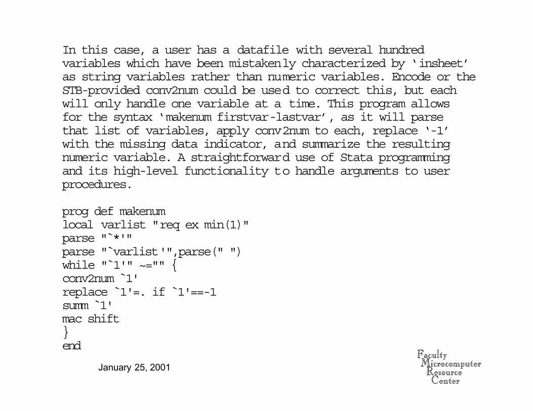
In this case, a user has a datafile with several hundredvariables which have been mistakenly characterized by ‘insheet’ as string variables rather than numeric variables. Encode or theSTB-provided conv2num could be used to correct this, but each will only handle one variable at a time. This program allows for the syntax ‘makenum firstvar-lastvar’, as it will parsethat list of variables, apply conv2num to each, replace ‘-1’with the missing data indicator, and summarize the resultingnumeric variable. A straightforward use of Stata programming and its high-level functionality to handle arguments to user procedures.

prog def makenumlocal varlist "req ex min(1)"parse "̀ *'"parse "̀ varlist'",parse(" ")while "̀ 1'" ~="" {conv2num ̀ 1'replace ̀ 1'=. if ̀ 1'==-1summ ̀ 1'mac shift}end

January 25, 2001

Getting Stata

� For students, faculty and staff at Boston College,desktop Stata (Mac/PowerMac, Win9x/NT/2000, orLinux) is available through the Stata GradPlan at asubstantial discount from the standard academicprice, with shipping costs waived. Ask me for aStata GradPlan brochure for details of the optionsavailable for software and documentation. Ordersare usually fulfilled within one business day afteryou fax or phone your order with payment toStataCorp.

Economic analysis with Stata 6.0/7 - fm · PDF fileEconomic analysis with Stata 6.0/7.0 ......

Documents

Transcript of Economic analysis with Stata 6.0/7 - fm · PDF fileEconomic analysis with Stata 6.0/7.0 ......