ECONOMIA degli INTERMEDIARI FINANZIARI AVANZATA

LECTURE 4

MODULO ASSET MANAGEMENT

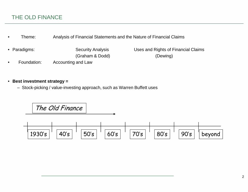
THE OLD FINANCE

• Theme: Analysis of Financial Statements and the Nature of Financial Claims

• Paradigms: Security Analysis Uses and Rights of Financial Claims(Graham & Dodd) (Dewing)

• Foundation: Accounting and Law

• Best investment strategy =– Stock-picking / value-investing approach, such as Warren Buffett uses

2

1930’s 40’s 50’s 60’s 70’s 80’s 90’s beyond

The Old Finance

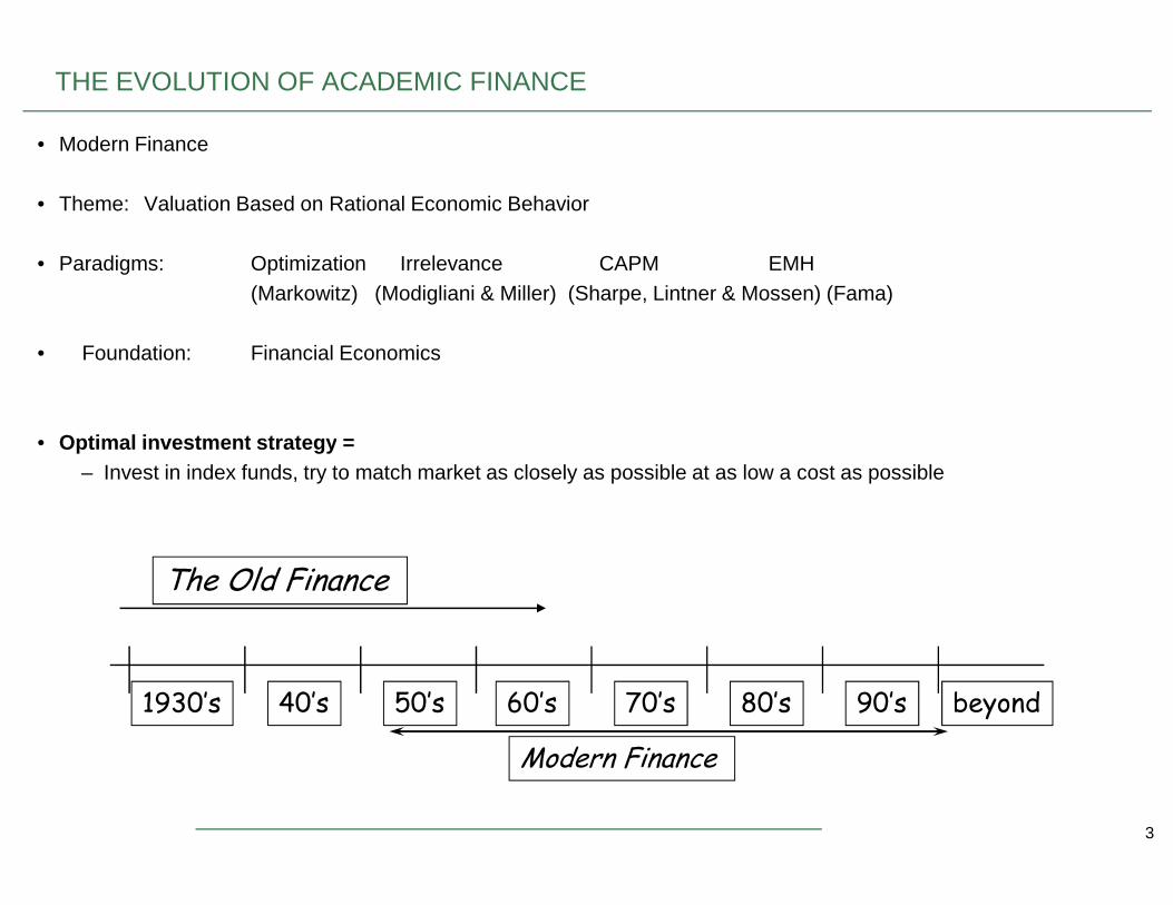
THE EVOLUTION OF ACADEMIC FINANCE

• Modern Finance

• Theme: Valuation Based on Rational Economic Behavior

• Paradigms: Optimization Irrelevance CAPM EMH(Markowitz) (Modigliani & Miller) (Sharpe, Lintner & Mossen) (Fama)

• Foundation: Financial Economics

• Optimal investment strategy =

3

1930’s 40’s 50’s 60’s 70’s 80’s 90’s beyond

The Old Finance

Modern Finance

• Optimal investment strategy =– Invest in index funds, try to match market as closely as possible at as low a cost as possible

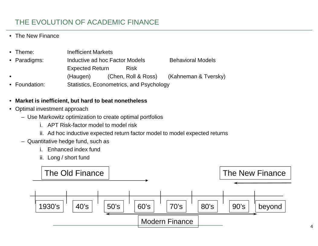
THE EVOLUTION OF ACADEMIC FINANCE

• The New Finance

• Theme: Inefficient Markets• Paradigms: Inductive ad hoc Factor Models Behavioral Models

Expected Return Risk• (Haugen) (Chen, Roll & Ross) (Kahneman & Tversky)• Foundation: Statistics, Econometrics, and Psychology

• Market is inefficient, but hard to beat nonetheless• Optimal investment approach

– Use Markowitz optimization to create optimal portfoliosi. APT Risk-factor model to model risk

4

1930’s 40’s 50’s 60’s 70’s 80’s 90’s beyond

The Old Finance

Modern Finance

The New Finance

i. APT Risk-factor model to model riskii. Ad hoc inductive expected return factor model to model expected returns

– Quantitative hedge fund, such asi. Enhanced index fundii. Long / short fund

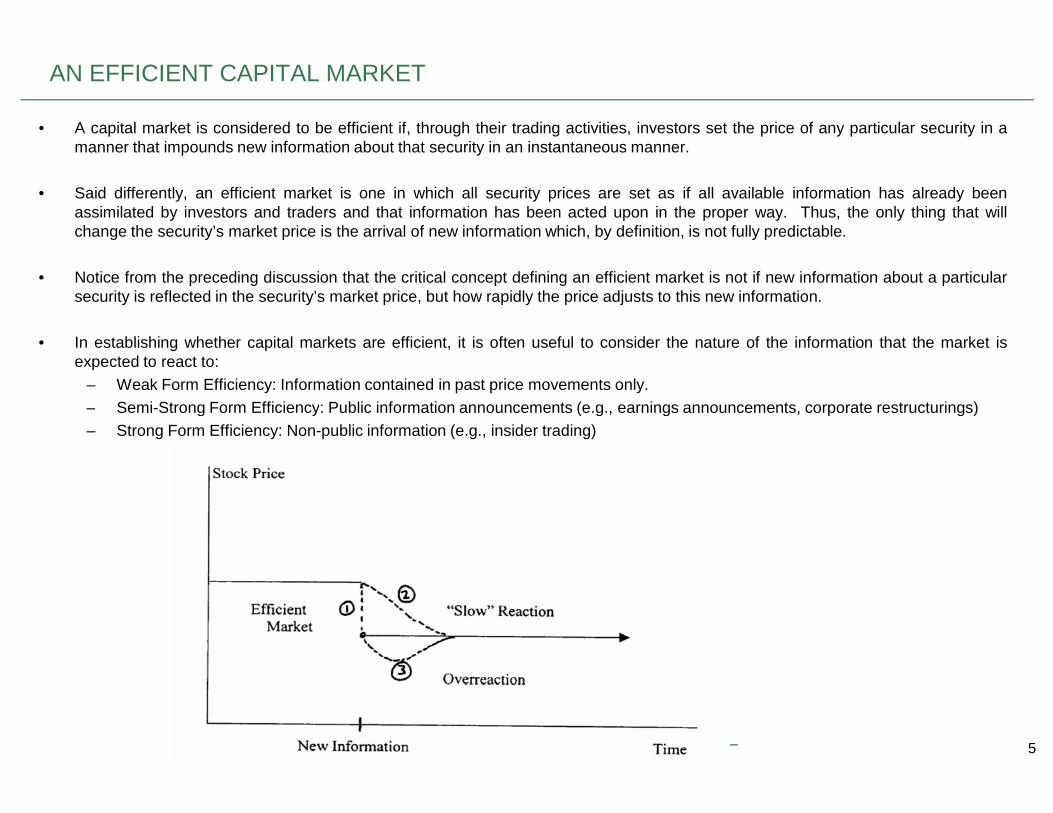
• A capital market is considered to be efficient if, through their trading activities, investors set the price of any particular security in amanner that impounds new information about that security in an instantaneous manner.

• Said differently, an efficient market is one in which all security prices are set as if all available information has already beenassimilated by investors and traders and that information has been acted upon in the proper way. Thus, the only thing that willchange the security’s market price is the arrival of new information which, by definition, is not fully predictable.

• Notice from the preceding discussion that the critical concept defining an efficient market is not if new information about a particularsecurity is reflected in the security’s market price, but how rapidly the price adjusts to this new information.

• In establishing whether capital markets are efficient, it is often useful to consider the nature of the information that the market isexpected to react to:

– Weak Form Efficiency: Information contained in past price movements only.– Semi-Strong Form Efficiency: Public information announcements (e.g., earnings announcements, corporate restructurings)

AN EFFICIENT CAPITAL MARKET

5

– Semi-Strong Form Efficiency: Public information announcements (e.g., earnings announcements, corporate restructurings)– Strong Form Efficiency: Non-public information (e.g., insider trading)

MARKET EFFICIENCY: IMPLICATIONS AND EVIDENCE

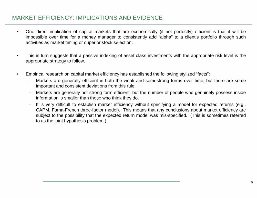
• One direct implication of capital markets that are economically (if not perfectly) efficient is that it will beimpossible over time for a money manager to consistently add “alpha” to a client’s portfolio through suchactivities as market timing or superior stock selection.

• This in turn suggests that a passive indexing of asset class investments with the appropriate risk level is theappropriate strategy to follow.

• Empirical research on capital market efficiency has established the following stylized “facts”:– Markets are generally efficient in both the weak and semi-strong forms over time, but there are some

important and consistent deviations from this rule.– Markets are generally not strong form efficient, but the number of people who genuinely possess inside

information is smaller than those who think they do.

6

information is smaller than those who think they do.– It is very difficult to establish market efficiency without specifying a model for expected returns (e.g.,

CAPM, Fama-French three-factor model). This means that any conclusions about market efficiency aresubject to the possibility that the expected return model was mis-specified. (This is sometimes referredto as the joint hypothesis problem.)

20.03

MARKET EFFICIENCY: IMPLICATIONS AND EVIDENCE

7

21.01

20.02

20.03

17.04

17.05

MARKET EFFICIENCY: IMPLICATIONS AND EVIDENCE

8

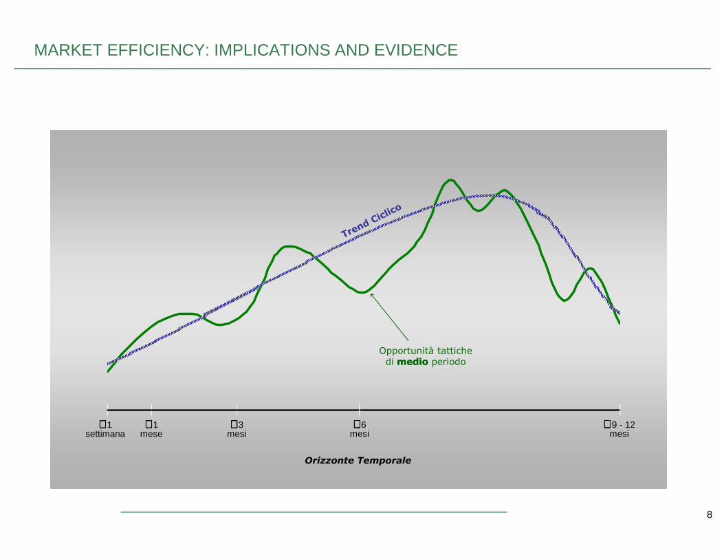
∼∼∼∼ 1settimana

∼∼∼∼ 1mese

∼∼∼∼ 3mesi

∼∼∼∼ 6mesi

∼ ∼ ∼ ∼ 9 - 12mesi

Orizzonte Temporale

Opportunità tattichedi mediomedio periodo

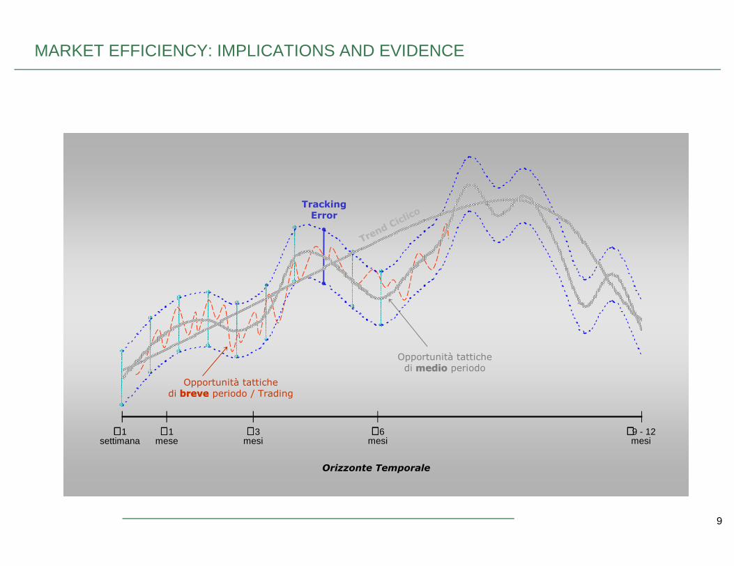
TrackingError

MARKET EFFICIENCY: IMPLICATIONS AND EVIDENCE

9

∼∼∼∼ 1settimana

∼∼∼∼ 1mese

∼∼∼∼ 3mesi

∼∼∼∼ 6mesi

∼∼∼∼9 - 12mesi

Orizzonte Temporale

Opportunità tattichedi brevebreve periodo / Trading

Opportunità tattichedi mediomedio periodo

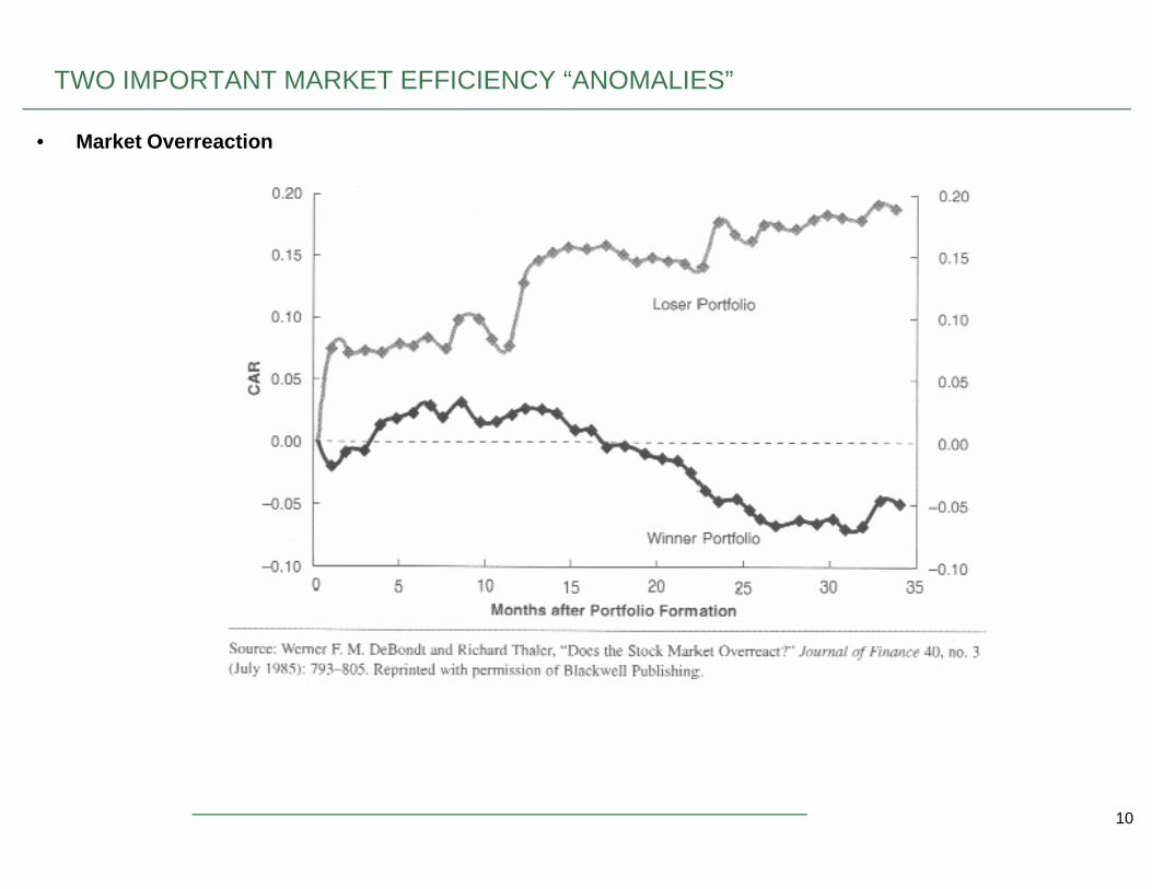
TWO IMPORTANT MARKET EFFICIENCY “ANOMALIES”

• Market Overreaction

10

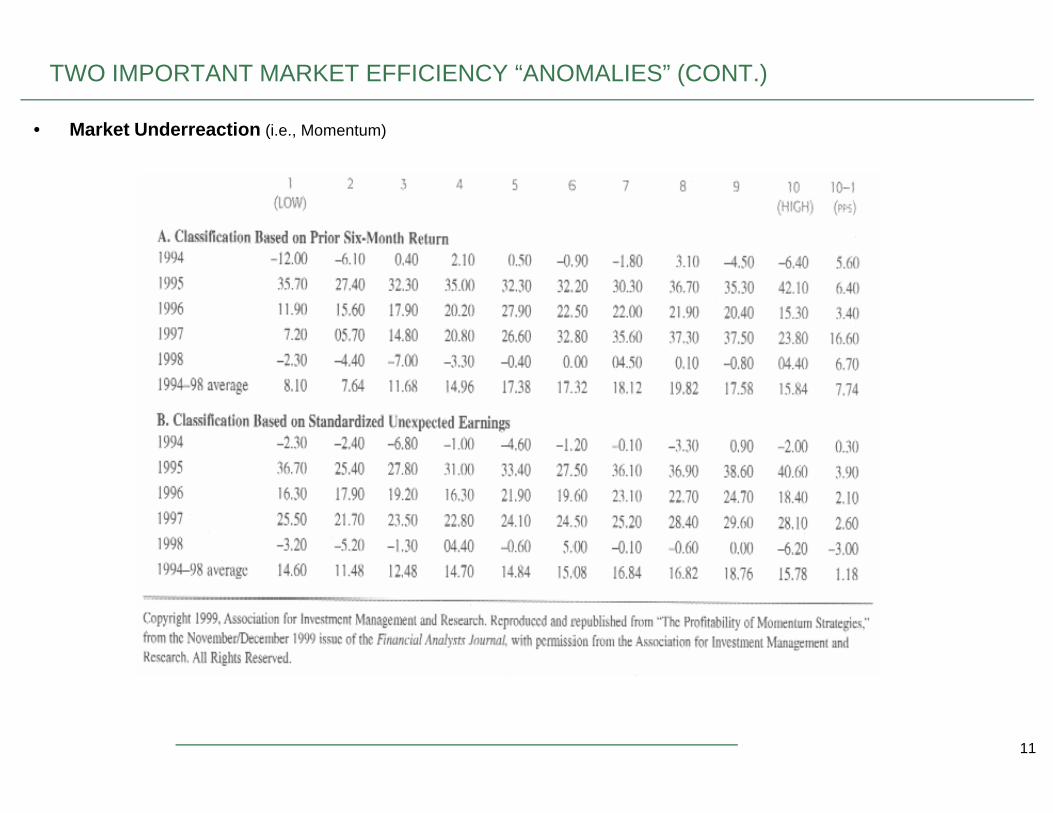
TWO IMPORTANT MARKET EFFICIENCY “ANOMALIES” (CONT.)

• Market Underreaction (i.e., Momentum)

11

BACKGROUND & DEFINITION

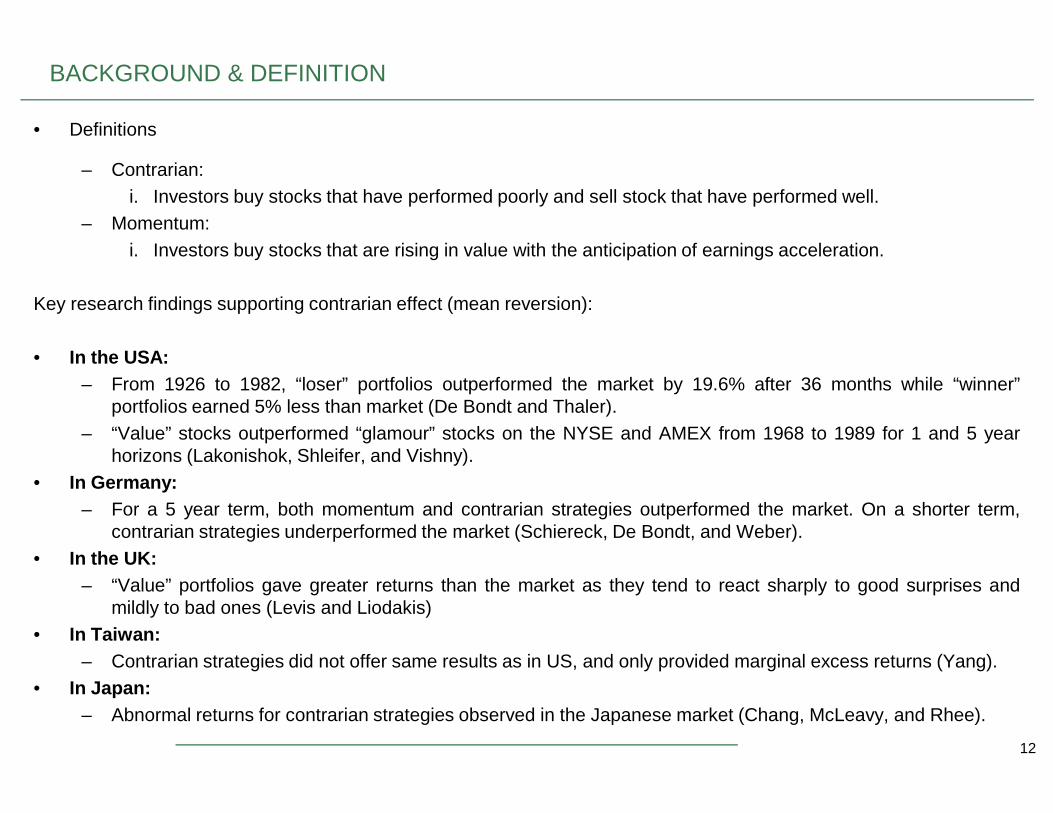
• Definitions

– Contrarian:i. Investors buy stocks that have performed poorly and sell stock that have performed well.

– Momentum:i. Investors buy stocks that are rising in value with the anticipation of earnings acceleration.

Key research findings supporting contrarian effect (mean reversion):

• In the USA:– From 1926 to 1982, “loser” portfolios outperformed the market by 19.6% after 36 months while “winner”

portfolios earned 5% less than market (De Bondt and Thaler).

12

portfolios earned 5% less than market (De Bondt and Thaler).– “Value” stocks outperformed “glamour” stocks on the NYSE and AMEX from 1968 to 1989 for 1 and 5 year

horizons (Lakonishok, Shleifer, and Vishny).• In Germany:

– For a 5 year term, both momentum and contrarian strategies outperformed the market. On a shorter term,contrarian strategies underperformed the market (Schiereck, De Bondt, and Weber).

• In the UK:– “Value” portfolios gave greater returns than the market as they tend to react sharply to good surprises and

mildly to bad ones (Levis and Liodakis)• In Taiwan:

– Contrarian strategies did not offer same results as in US, and only provided marginal excess returns (Yang).• In Japan:

– Abnormal returns for contrarian strategies observed in the Japanese market (Chang, McLeavy, and Rhee).

MARKET ANOMALIES: MOMENTUM EFFECT

• Momentum profitability poses a strong challenge to the theory of asset pricing – momentum effect is the mostchallenging asset pricing anomaly

• A momentum effect captures the short-term (6 to 12 months) return continuation effect that stocks with high returnsover the past three to 12 months tend to outperform in the future (Jegadeesh & Titman, JoF 1993).

• Very simple trading strategy – portfolio is constructed based on cumulative return criterion over certain time-horizon

• Historically momentum strategy earned profits of about 1% per month over the following 12 months.

• The profitability cannot be explained with the existing multi-factor models and macroeconomic-based riskexplanations

13

explanations

MOMENTUM EFFECT POSSIBILE EXPLANATION

• What is the real cause of the momentum effect?

• Results are spurios or product of “data mining” – this argument has been neutralized through consistent findings ofthe momentum effect in various markets and across different time periods

• Results are compensation for risk bearing – current findings are inconclusive and contradictory

• Irrational behavior of investors is causing momentum – behavioral theories of overreaction and underreaction havealso been formulated

14

IMPACT OF THE MOMENTUM EFFECT ON OTHER LINKED AREAS

unresolved issues in current research on the momentum effect

• “Industry Effect” – is this similar phenomenon linked or independent of the momentum effect; if yes, to what degreeand why?

• What (multi-factor) models shall be used as a benchmark to estimate risk-adjusted momentum profits?

• Some findings point out that the momentum effect is mostly based on the persistence of the winners – what are thekey characteristics of stocks in extreme portfolios and how they impact the profitability?

• How large is the impact of transaction cost?

15

• How more profitable strategies can be created? –Derivation of optimized-weight strategy based on optimization ofcertain properties of stocks in winner and loser portfolios.

ACTIVE EQUITY MANAGEMENT: TECHNICAL VS. FUNDAMENTAL APPROACHES

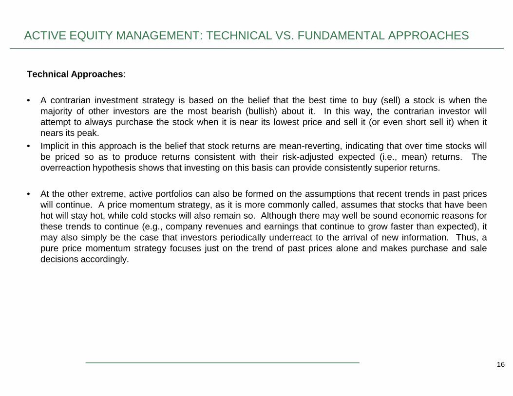
Technical Approaches:

• A contrarian investment strategy is based on the belief that the best time to buy (sell) a stock is when themajority of other investors are the most bearish (bullish) about it. In this way, the contrarian investor willattempt to always purchase the stock when it is near its lowest price and sell it (or even short sell it) when itnears its peak.

• Implicit in this approach is the belief that stock returns are mean-reverting, indicating that over time stocks willbe priced so as to produce returns consistent with their risk-adjusted expected (i.e., mean) returns. Theoverreaction hypothesis shows that investing on this basis can provide consistently superior returns.

• At the other extreme, active portfolios can also be formed on the assumptions that recent trends in past prices

16

• At the other extreme, active portfolios can also be formed on the assumptions that recent trends in past priceswill continue. A price momentum strategy, as it is more commonly called, assumes that stocks that have beenhot will stay hot, while cold stocks will also remain so. Although there may well be sound economic reasons forthese trends to continue (e.g., company revenues and earnings that continue to grow faster than expected), itmay also simply be the case that investors periodically underreact to the arrival of new information. Thus, apure price momentum strategy focuses just on the trend of past prices alone and makes purchase and saledecisions accordingly.

ACTIVE EQUITY MANAGEMENT: TECHNICAL VS. FUNDAMENTAL APPROACHES

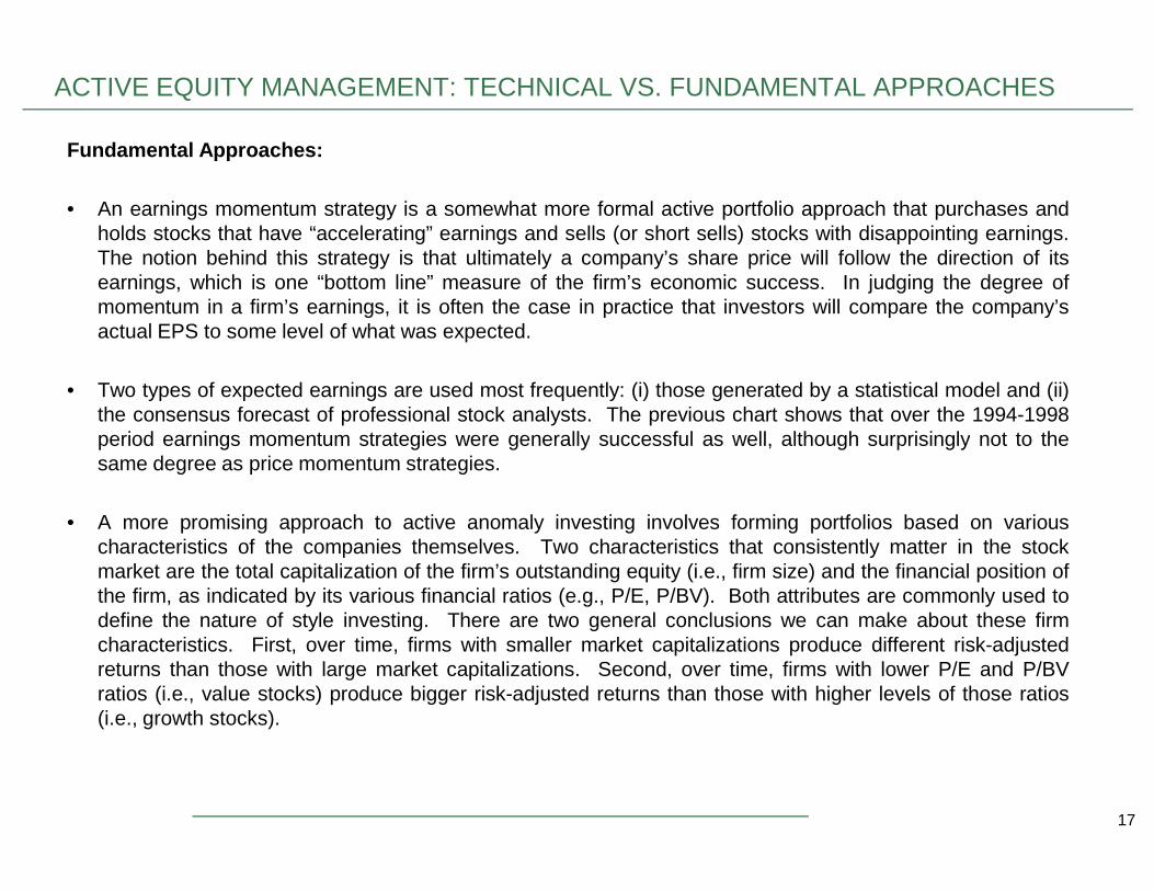
Fundamental Approaches:

• An earnings momentum strategy is a somewhat more formal active portfolio approach that purchases andholds stocks that have “accelerating” earnings and sells (or short sells) stocks with disappointing earnings.The notion behind this strategy is that ultimately a company’s share price will follow the direction of itsearnings, which is one “bottom line” measure of the firm’s economic success. In judging the degree ofmomentum in a firm’s earnings, it is often the case in practice that investors will compare the company’sactual EPS to some level of what was expected.

• Two types of expected earnings are used most frequently: (i) those generated by a statistical model and (ii)the consensus forecast of professional stock analysts. The previous chart shows that over the 1994-1998period earnings momentum strategies were generally successful as well, although surprisingly not to the

17

period earnings momentum strategies were generally successful as well, although surprisingly not to thesame degree as price momentum strategies.

• A more promising approach to active anomaly investing involves forming portfolios based on variouscharacteristics of the companies themselves. Two characteristics that consistently matter in the stockmarket are the total capitalization of the firm’s outstanding equity (i.e., firm size) and the financial position ofthe firm, as indicated by its various financial ratios (e.g., P/E, P/BV). Both attributes are commonly used todefine the nature of style investing. There are two general conclusions we can make about these firmcharacteristics. First, over time, firms with smaller market capitalizations produce different risk-adjustedreturns than those with large market capitalizations. Second, over time, firms with lower P/E and P/BVratios (i.e., value stocks) produce bigger risk-adjusted returns than those with higher levels of those ratios(i.e., growth stocks).

EXAMPLE 1: JAPAN MARKET 1994-2004

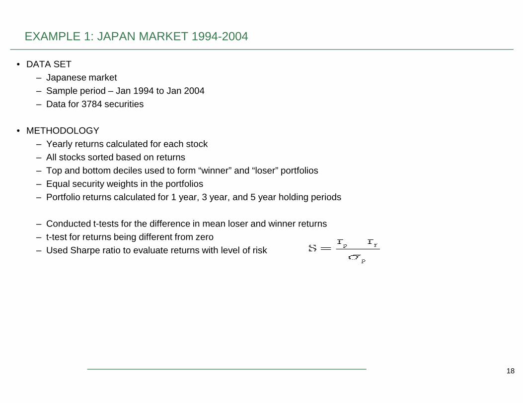
• DATA SET– Japanese market– Sample period – Jan 1994 to Jan 2004– Data for 3784 securities

• METHODOLOGY– Yearly returns calculated for each stock– All stocks sorted based on returns– Top and bottom deciles used to form “winner” and “loser” portfolios– Equal security weights in the portfolios– Portfolio returns calculated for 1 year, 3 year, and 5 year holding periods

18

– Portfolio returns calculated for 1 year, 3 year, and 5 year holding periods

– Conducted t-tests for the difference in mean loser and winner returns– t-test for returns being different from zero– Used Sharpe ratio to evaluate returns with level of risk

DATA SET

Japan Nikkei Index 1994-2004

5,000

7,000

9,000

11,000

13,000

15,000

17,000

19,000

21,000

1994 1995 1996 1997 1998 1999 2000 2001 2002 2003 2004

Year

Lev

el

Nikkei vs S&P 500 and Hang Seng

Nikkei 225 (-47%)

19

4/1/

94

4/1/

95

4/1/

96

4/1/

97

4/1/

98

4/1/

99

4/1/

00

4/1/

01

4/1/

02

4/1/

03

4/1/

04

Nikkei 225 (-47%)

S&P 500 (+135%)

Hang Seng (+11%)

RESULTS & CONCLUSIONS

1 year 3 year 5 year

Full Sample

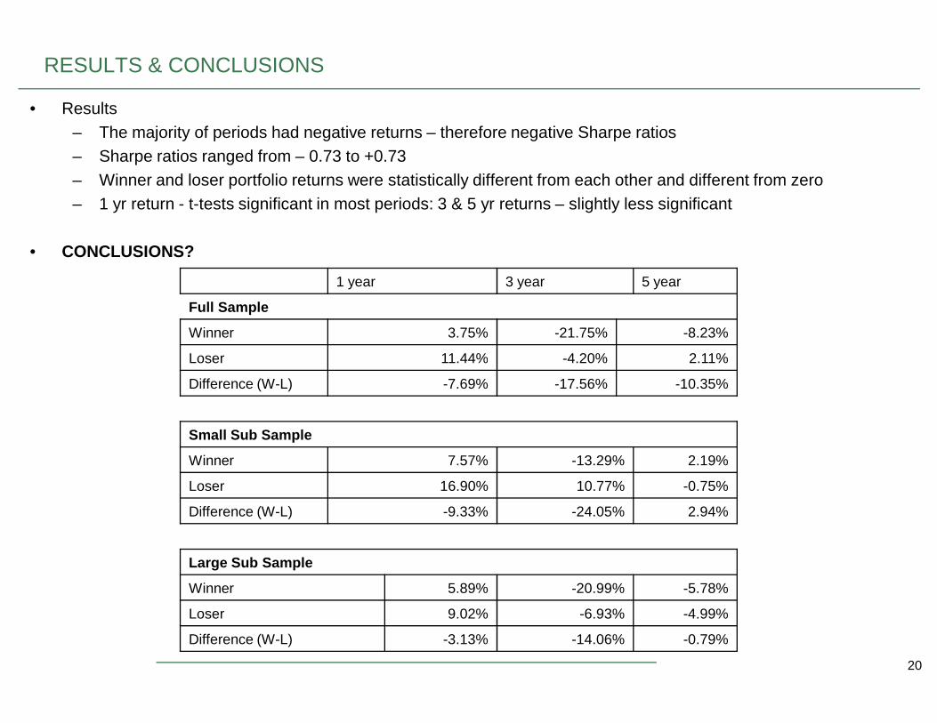
Winner 3.75% -21.75% -8.23%

Loser 11.44% -4.20% 2.11%

• Results– The majority of periods had negative returns – therefore negative Sharpe ratios– Sharpe ratios ranged from – 0.73 to +0.73– Winner and loser portfolio returns were statistically different from each other and different from zero– 1 yr return - t-tests significant in most periods: 3 & 5 yr returns – slightly less significant

• CONCLUSIONS?

20

Loser 11.44% -4.20% 2.11%

Difference (W-L) -7.69% -17.56% -10.35%

Small Sub Sample

Winner 7.57% -13.29% 2.19%

Loser 16.90% 10.77% -0.75%

Difference (W-L) -9.33% -24.05% 2.94%

Large Sub Sample

Winner 5.89% -20.99% -5.78%

Loser 9.02% -6.93% -4.99%

Difference (W-L) -3.13% -14.06% -0.79%

EXAMPLE 1: US MARKET 1992-2003

• Data and Methodology

• We use daily data of 382 stocks included in the S&P Index in the period January 1, 1992 to December 31, 2003.(stocks with equal and complete return history)

• Four “J-month/K-month” strategíes based on the ranking and holding periods of 6 and 12 months are examined (i.e.,6/6, 6/12, 12/6 and 12/12 strategy)

• Strategies are applied to non-overlapping K-month investment horizons (I.e., positions are held for K-months afterwhich the portfolio is rebalanced)

• We also examine strategies with one-month holding periods and with one-month gap between ranking and holingperiod

21

period

• Zero-investment portfolio is constructed at the end of each ranking period by simultaneously selling winners andlosers

• Stocks with highest value of risk-adjusted criterion constitute winner portfolio (e.g., highest decile) and those withlowest the loser portfolio

• Performance of the momentum portfolio (winner – loser) is evaluated at the end of each holding or investment period

MODIFICATION OF THE DECISION CRITERIA FOR PORTFOLIO CONSTRUCTION

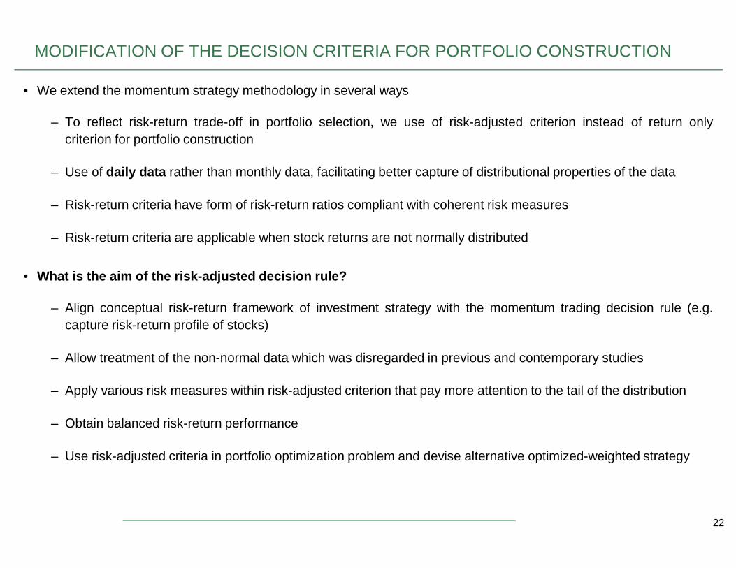
• We extend the momentum strategy methodology in several ways

– To reflect risk-return trade-off in portfolio selection, we use of risk-adjusted criterion instead of return onlycriterion for portfolio construction

– Use of daily data rather than monthly data, facilitating better capture of distributional properties of the data

– Risk-return criteria have form of risk-return ratios compliant with coherent risk measures

– Risk-return criteria are applicable when stock returns are not normally distributed

• What is the aim of the risk-adjusted decision rule?

22

– Align conceptual risk-return framework of investment strategy with the momentum trading decision rule (e.g.capture risk-return profile of stocks)

– Allow treatment of the non-normal data which was disregarded in previous and contemporary studies

– Apply various risk measures within risk-adjusted criterion that pay more attention to the tail of the distribution

– Obtain balanced risk-return performance

– Use risk-adjusted criteria in portfolio optimization problem and devise alternative optimized-weighted strategy

RISK-ADJUSTED CRITERION: BENEFIT

• What we would like to examine?

• Whether the risk-adjusted criteria can generate more profitable strategies than those based on simple cumulativereturn criterion

• What is the appropriate risk measure embedded in a risk-return criterion that obtains the best results (e.g., Variance,ETL)

• Evaluate and compare performance of ratios based on different distributional assumption and measures of risk

• Which criterion gives the most robust strategy regarding transaction costs ?

23

• What is the marginal benefit of the optimized-weighted strategy?

TREATMENT OF NON-NORMAL DATA

Normal distribution is not a realistic assumption for stock returns

• High empirical kurtosis ⇒ heavy tailedness

• Asymmetric empirical distribution

• Slowly decaying correlation of squared returns ⇒ long-range dependence

• Heteroskedaticity (volatility clustering)

24

OPTIMIZATION STRUCTURE

Optimizing weights within winner and loser portfolios may lead to improvement in performance over usual equally-weighted strategies

• Risk-return ratio (Sharpe) is used as an objective function in the optimization

• At the rebalancing time points, we solve two optimization problems using the risk-return ratio ρ

• The optimal risky portfolios are given by the portfolio that maximizes the criterion measure ρ(.) for winners andminimizes the same measure for losers.

• By solving optimization problems, we adjust the proportion of stocks in the winner and loser portfolio according to the

25

• By solving optimization problems, we adjust the proportion of stocks in the winner and loser portfolio according to theweights obtained

• We compare the profits of an optimized-weighted strategies with those of an equal-weighted strategy

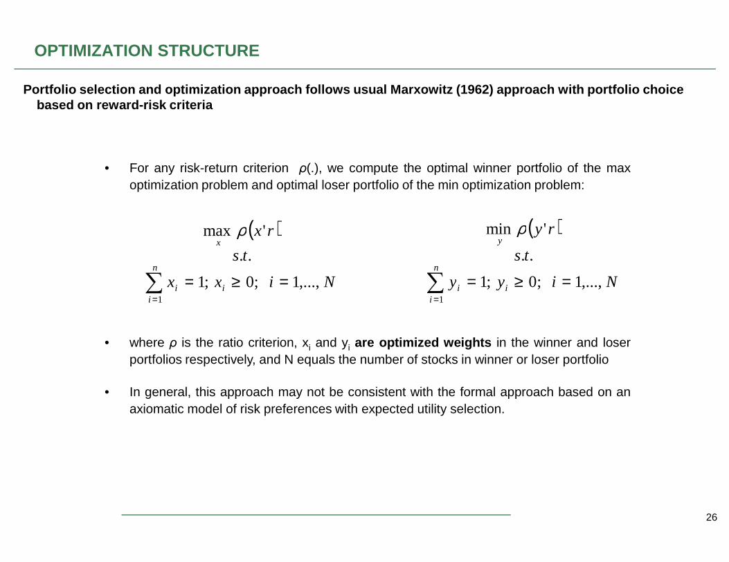
Portfolio selection and optimization approach follows usual Marxowitz (1962) approach with portfolio choice based on reward-risk criteria

• For any risk-return criterion ρ(.), we compute the optimal winner portfolio of the maxoptimization problem and optimal loser portfolio of the min optimization problem:

( )

Nixx

ts

rx

n

x

,...,1;0;1

..

'max

=≥=∑

ρ ( )

Niyy

ts

ry

n

y

,...,1;0;1

..

'min

=≥=∑

ρ

OPTIMIZATION STRUCTURE

26

• where ρ is the ratio criterion, xi and yi are optimized weights in the winner and loserportfolios respectively, and N equals the number of stocks in winner or loser portfolio

• In general, this approach may not be consistent with the formal approach based on anaxiomatic model of risk preferences with expected utility selection.

Nixx ii

i ,...,1;0;11

=≥=∑=

Niyy ii

i ,...,1;0;11

=≥=∑=

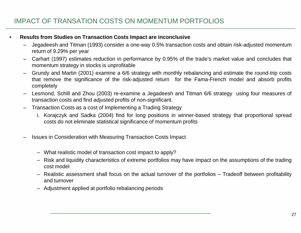
IMPACT OF TRANSATION COSTS ON MOMENTUM PORTFOLIOS

• Results from Studies on Transaction Costs Impact are inconclusive– Jegadeesh and Titman (1993) consider a one-way 0.5% transaction costs and obtain risk-adjusted momentum

return of 9.29% per year– Carhart (1997) estimates reduction in performance by 0.95% of the trade’s market value and concludes that

momentum strategy in stocks is unprofitable– Grundy and Martin (2001) examine a 6/6 strategy with monthly rebalancing and estimate the round-trip costs

that remove the significance of the risk-adjusted return for the Fama-French model and absorb profitscompletely

– Lesmond, Schill and Zhou (2003) re-examine a Jegadeesh and Titman 6/6 strategy using four measures oftransaction costs and find adjusted profits of non-significant.

– Transaction Costs as a cost of Implementing a Trading Strategyi. Korajczyk and Sadka (2004) find for long positions in winner-based strategy that proportional spread

27

i. Korajczyk and Sadka (2004) find for long positions in winner-based strategy that proportional spreadcosts do not eliminate statistical significance of momentum profits

– Issues in Consideration with Measuring Transaction Costs Impact

– What realistic model of transaction cost impact to apply?– Risk and liquidity characteristics of extreme portfolios may have impact on the assumptions of the trading

cost model– Realistic assessment shall focus on the actual turnover of the portfolios – Tradeoff between profitability

and turnover– Adjustment applied at portfolio rebalancing periods

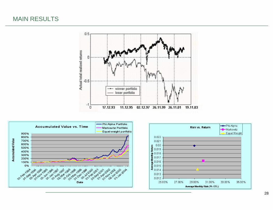
MAIN RESULTS

28

TOOLS OF “TECHNICAL ANALYSIS”

• Contrarian Opinion– The theory that if people are very optimistic, that is a predictor of falling prices for the market, and…– If people are very pessimistic, that is a predictor of rising prices

• We covered Contrarian Strategy already in Investment Strategies– Buy when others are selling– Sell when others are buying– The problem is the market historically has gone up three times more than it goes down

• Silly Theories & Oddities– Super Bowl Theory

29

i. National League Wins – bullishii. American League Wins – bearish

– Hemlines of skirtsi. Mini skirts – bullishii. Long skirts – bearish

– The Monday Effect– The January Effect– September and October

– Worst months of the year

• “Bear markets are born of pessimism, grow on skepticism, mature on optimism and die on euphoria. The timeof maximum pessimism is the best time to buy.” f. Templeton