Econometrics Using Stata - ReSAKSS Asia · Introduction to Stata • What is Stata? –A computer...

INTRODUCTION TO USING STATA FOR

ECONOMETRICS

November 14-18, 2016

Dushanbe, Tajikistan

Allen Park and Jarilkasin Ilyasov

Purpose of the Course

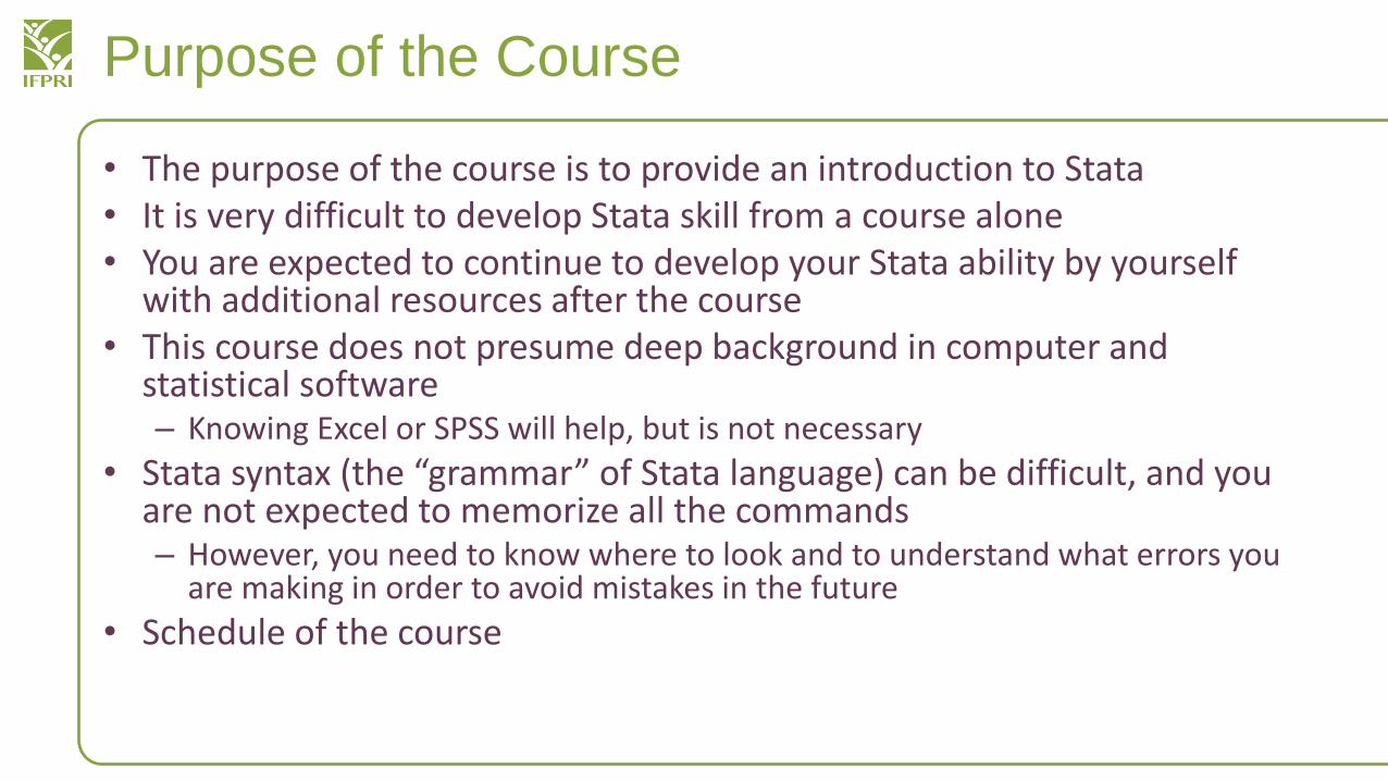
• The purpose of the course is to provide an introduction to Stata• It is very difficult to develop Stata skill from a course alone• You are expected to continue to develop your Stata ability by yourself

with additional resources after the course• This course does not presume deep background in computer and

statistical software– Knowing Excel or SPSS will help, but is not necessary

• Stata syntax (the “grammar” of Stata language) can be difficult, and you are not expected to memorize all the commands– However, you need to know where to look and to understand what errors you

are making in order to avoid mistakes in the future

• Schedule of the course

Introduction to Stata

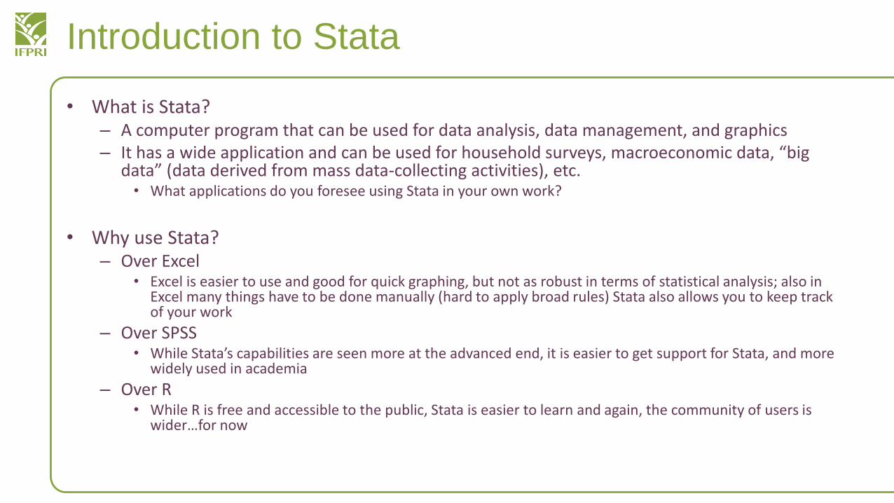
• What is Stata?– A computer program that can be used for data analysis, data management, and graphics– It has a wide application and can be used for household surveys, macroeconomic data, “big

data” (data derived from mass data-collecting activities), etc.• What applications do you foresee using Stata in your own work?

• Why use Stata?– Over Excel

• Excel is easier to use and good for quick graphing, but not as robust in terms of statistical analysis; also in Excel many things have to be done manually (hard to apply broad rules) Stata also allows you to keep track of your work

– Over SPSS• While Stata’s capabilities are seen more at the advanced end, it is easier to get support for Stata, and more

widely used in academia

– Over R• While R is free and accessible to the public, Stata is easier to learn and again, the community of users is

wider…for now

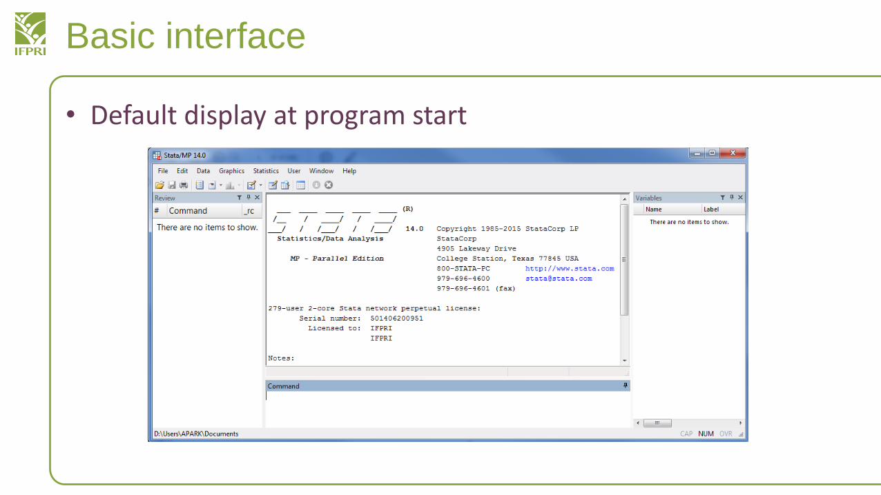
Basic interface

• Default display at program start

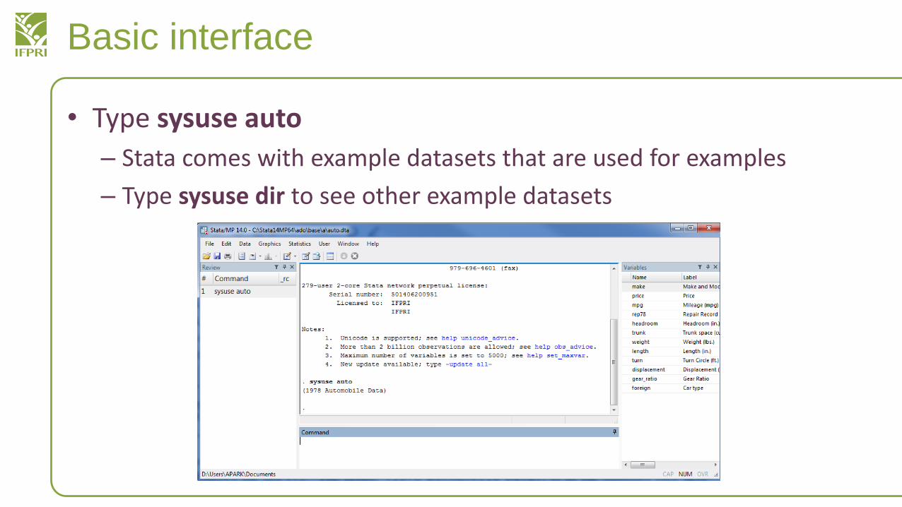
Basic interface

• Type sysuse auto

– Stata comes with example datasets that are used for examples

– Type sysuse dir to see other example datasets

Basic Interface Summary

• Main Window– Shows the result of your actions

• Command Line– Where you type in your actions

• Variables– Lists variables associated with the dataset

• Review Window– Tracks the commands you enter

• Directory bar

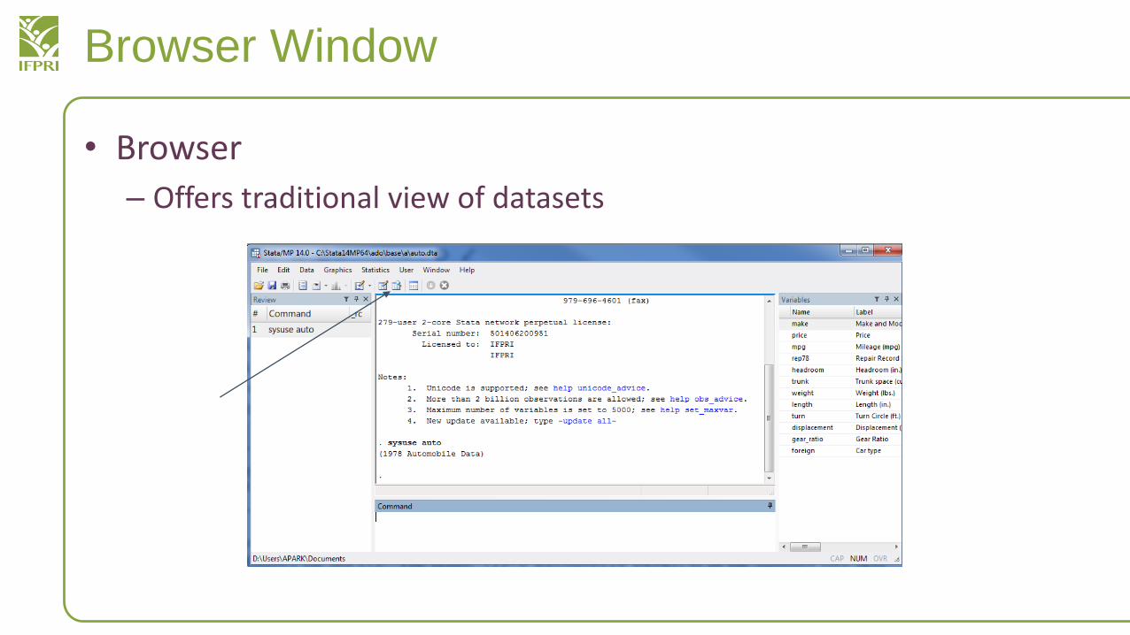
Browser Window

• Browser

– Offers traditional view of datasets

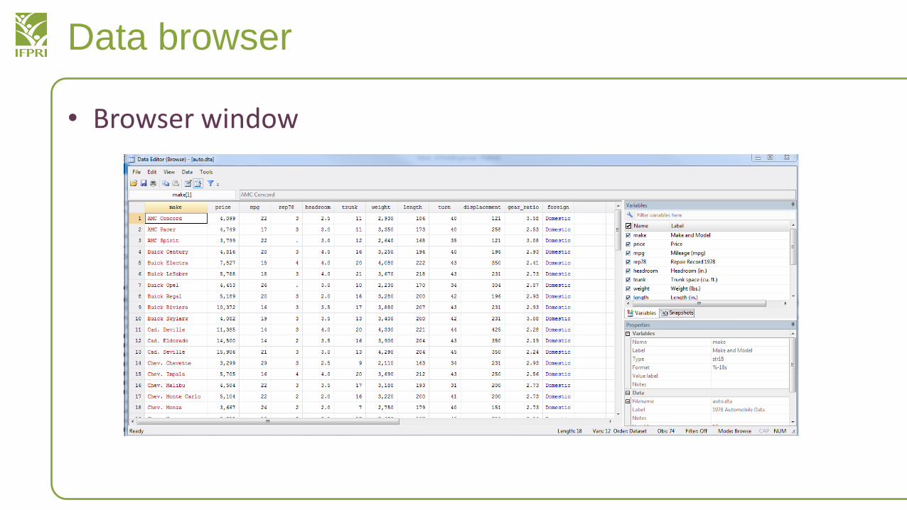
Data browser

• Browser window

Exercises

Browser Window- How many cars are listed there?- What is the most expensive car that is listed?- How many variables are listed?

Variables Tab in the Browser Window- Can you read the label for “foreign?”- Can you hide everything except for make and price?

From the main command window- How can you call up the browser window?- browse

Basic File Management

• dir – “directory,” shows all the files that are in the folder

– Can you find which folder it is currently in?

• pwd – “present working directory”

• Create a folder on Windows where you want all these training files to be placed

• cd – “change directory,” changes the folder where you are working from

Basic syntax and mathematical operators

• disp = display– What happens when you type disp “Hello”– What happens when you type disp “Hello” “world”– What happens when you type disp hello?– Use “ ” when you are describing string characters (text)

• Otherwise, Stata will think you are talking about variables

• Mathematical operators include: + - * / ^ ( )– What happens when you display 4– What happens when you display 4 + 7– How would you display (21-12)*3

– How would you display (36+12)−42

(4 ∗ 2)

Basic data commands

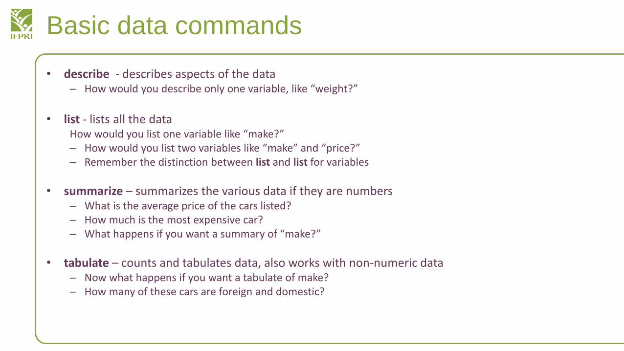
• describe - describes aspects of the data– How would you describe only one variable, like “weight?”

• list - lists all the dataHow would you list one variable like “make?”– How would you list two variables like “make” and “price?”– Remember the distinction between list and list for variables

• summarize – summarizes the various data if they are numbers– What is the average price of the cars listed? – How much is the most expensive car?– What happens if you want a summary of “make?”

• tabulate – counts and tabulates data, also works with non-numeric data– Now what happens if you want a tabulate of make?– How many of these cars are foreign and domestic?

Logical operators

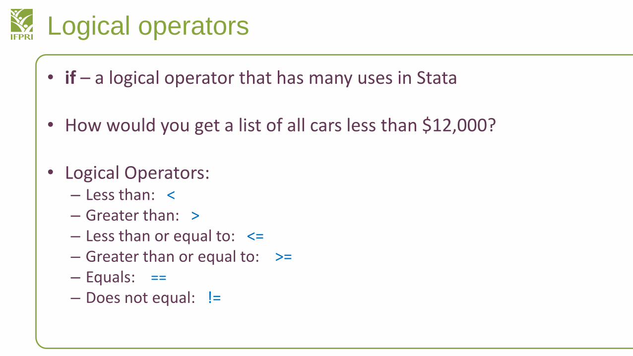
• if – a logical operator that has many uses in Stata

• How would you get a list of all cars less than $12,000?

• Logical Operators: – Less than: <– Greater than: >– Less than or equal to: <=– Greater than or equal to: >=– Equals: ==

– Does not equal: !=

Exercises

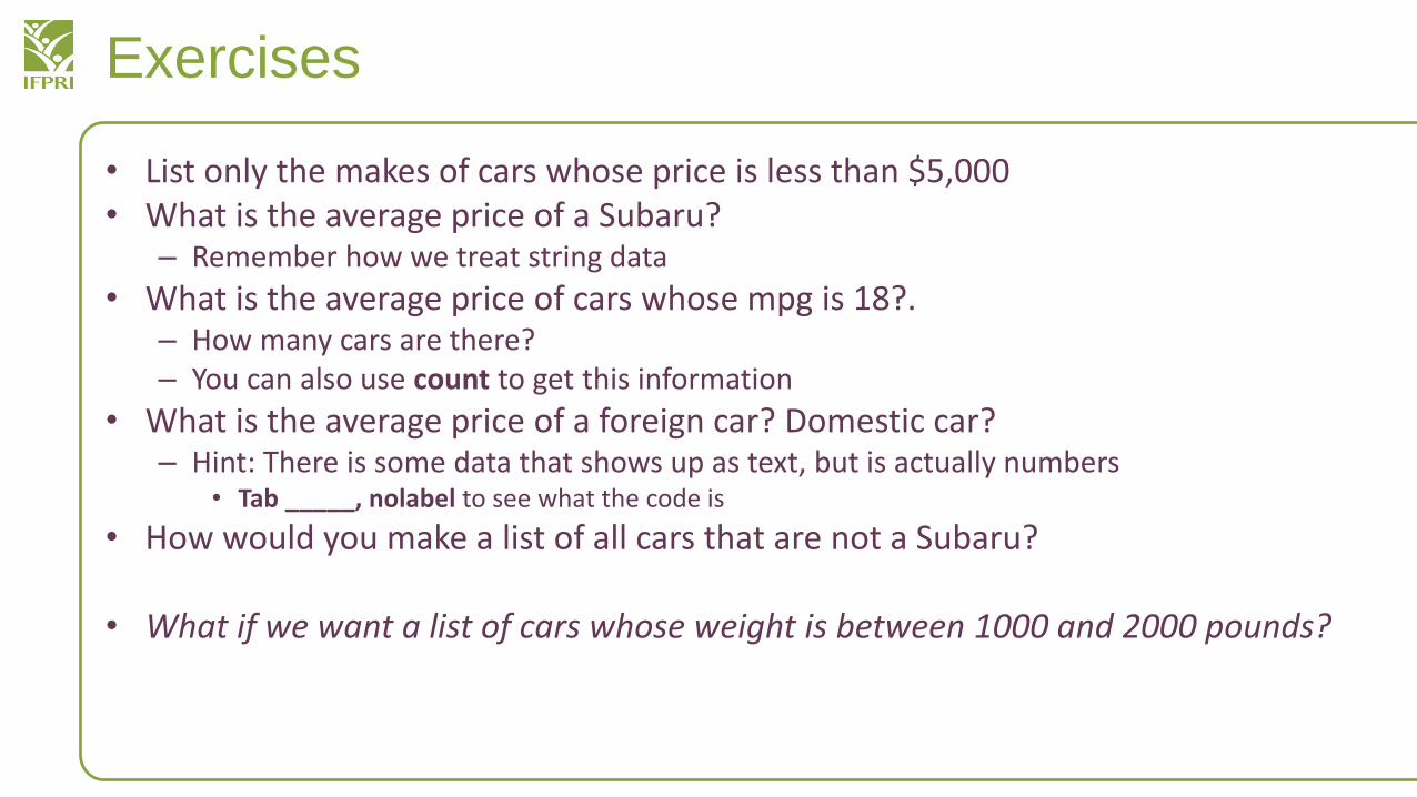
• List only the makes of cars whose price is less than $5,000• What is the average price of a Subaru?

– Remember how we treat string data

• What is the average price of cars whose mpg is 18?.– How many cars are there?– You can also use count to get this information

• What is the average price of a foreign car? Domestic car?– Hint: There is some data that shows up as text, but is actually numbers

• Tab _____, nolabel to see what the code is

• How would you make a list of all cars that are not a Subaru?

• What if we want a list of cars whose weight is between 1000 and 2000 pounds?

Logical operators: “and,” “or”

• & • |

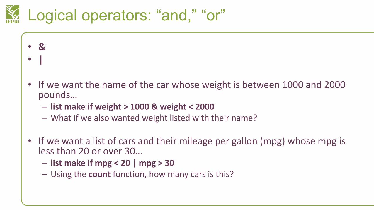
• If we want the name of the car whose weight is between 1000 and 2000 pounds…– list make if weight > 1000 & weight < 2000– What if we also wanted weight listed with their name?

• If we want a list of cars and their mileage per gallon (mpg) whose mpg is less than 20 or over 30…– list make if mpg < 20 | mpg > 30– Using the count function, how many cars is this?

Homework Assignment

• Use gnp96.dta, a dataset showing GNP of an unknown country over time

– sysuse gnp96.dta, clear

1. Using any method, how many observations are there?

2. What are the names of the two variables?

3. What is the meaning of the second variable? (Name of the label)

4. What is the average figure of the GNP over the various observations?

Contact information

• Dr. Kamiljon Akramov– ([email protected])

• Jarilkasin Ilyasov– ([email protected])

• Allen Park – ([email protected])

mailto:[email protected]



Review of Day 1

• Basic interface

• Mathematical operators

• Data commands (describe, summarize, tabulate, list)

• Basic logical operators (and, or)

Preview of Day 2

• File management

• Help resources

• Variable management

Quick Note: Dummy Variables

• What is the average price of a domestic car?– There was no variable called “domestic,” only “foreign”

• Dummy variables are used to describe binary data – 1 or 0

• If we had a binary variable named:– Left, what does left == 0 mean?

– Male, what does male == 0 mean?

– Big, what does big == 1 mean?

Quick Note: Value Labels for Coded Data

• Remember that some data is coded as a number, but when you tab it, it comes out as a description

– This is because there is a value label (we will go over this later)

• numlabel, add – allows you to avoid this confusion

– Type this and then tabulate foreign again

• How do you think we can undo what we just did?

– numlabel, remove

Quick Note: Review of Data and Logic

• The five files are part of one survey done in Tajikistan: household (general household information), hhmembers (list of family members), food (food consumption information), agri (agricultural information), migration (migration)

• Open the household file

• Look at a description of the dataset

Quick Note: Review of Data and Logic

• What is the average household size of the members in our sample?

• Can you add labels to data that has been coded as a number?

• Can you tabulate the number of households in each district?

• What is the average household size in Yovon district?

• Can you list the household IDs in the smallest district?

• Can you compare the average household size for urban and rural households?

• sum ______, detail – shows summarize in more detail

File management: Saving

• sysuse auto, clear - we have not made any major changes to the file yet, but let us save a version of this data

• Type save training.dta to save the file

• Look at the directory bar in the bottom-left corner, this is the folder your file will be saved to

– Using Windows, look up the location of the file you just created

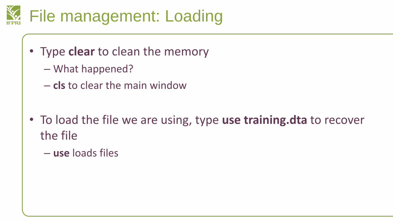
File management: Loading

• Type clear to clean the memory

– What happened?

– cls to clear the main window

• To load the file we are using, type use training.dta to recover the file

– use loads files

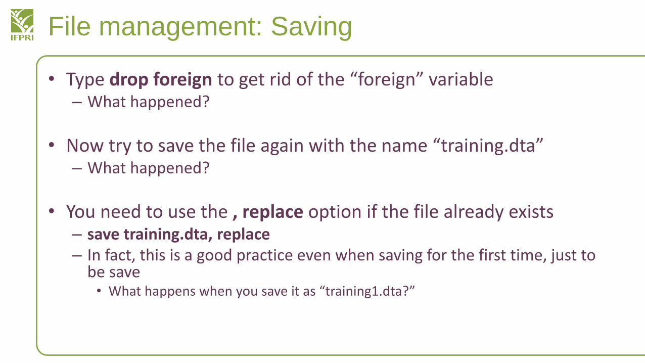
File management: Saving

• Type drop foreign to get rid of the “foreign” variable– What happened?

• Now try to save the file again with the name “training.dta”– What happened?

• You need to use the , replace option if the file already exists– save training.dta, replace– In fact, this is a good practice even when saving for the first time, just to

be save• What happens when you save it as “training1.dta?”

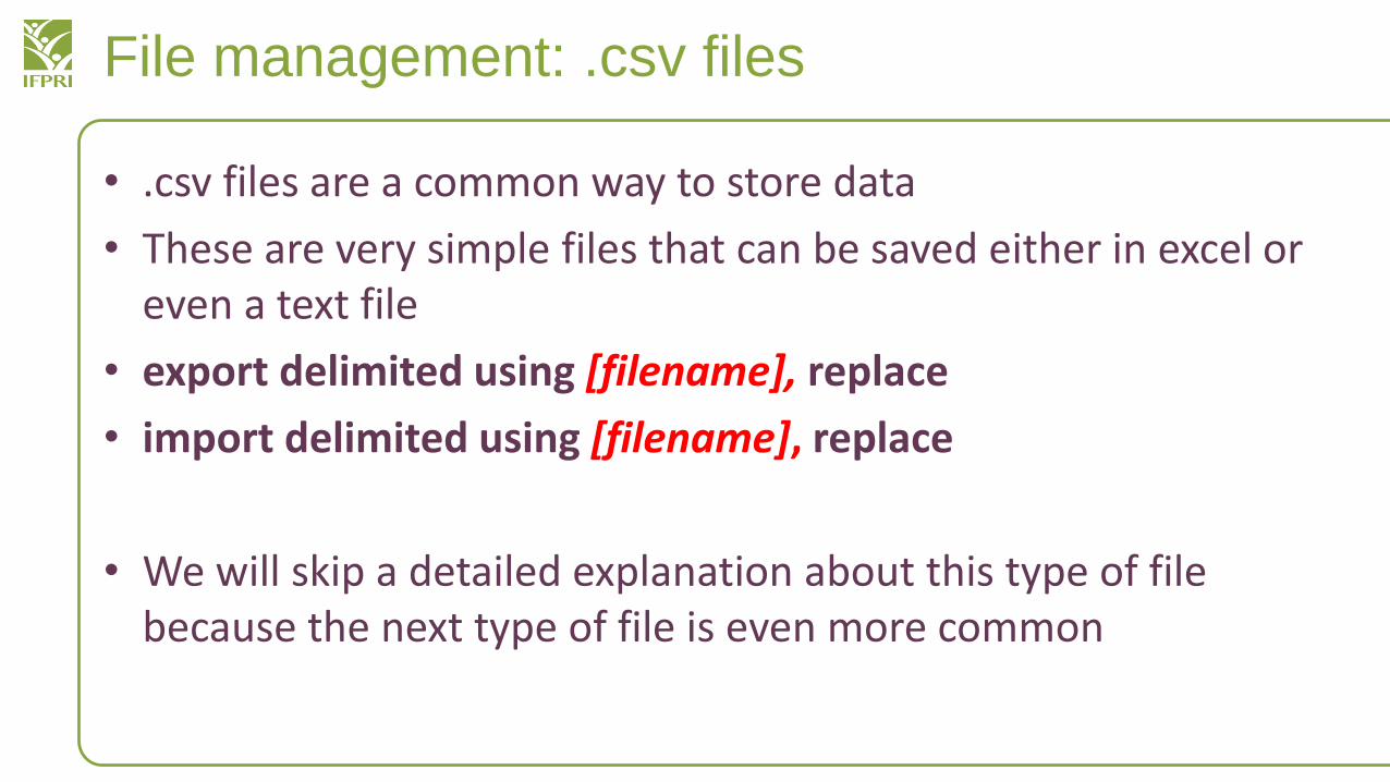
File management: .csv files

• .csv files are a common way to store data

• These are very simple files that can be saved either in excel or even a text file

• export delimited using [filename], replace

• import delimited using [filename], replace

• We will skip a detailed explanation about this type of file because the next type of file is even more common

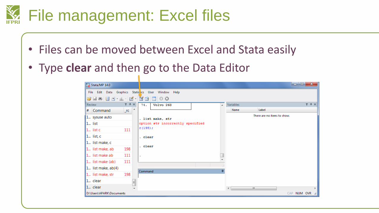
File management: Excel files

• Files can be moved between Excel and Stata easily

• Type clear and then go to the Data Editor


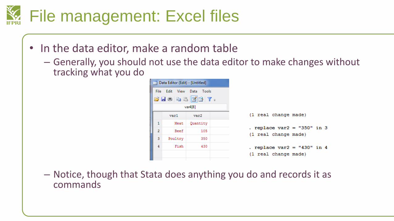
• In the data editor, make a random table – Generally, you should not use the data editor to make changes without

tracking what you do

– Notice, though that Stata does anything you do and records it as commands


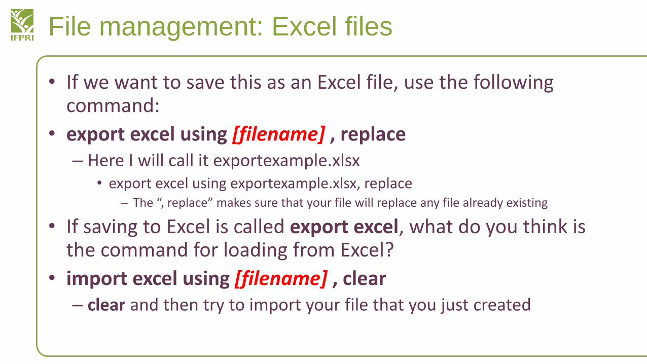
• If we want to save this as an Excel file, use the following command:

• export excel using [filename] , replace– Here I will call it exportexample.xlsx

• export excel using exportexample.xlsx, replace– The “, replace” makes sure that your file will replace any file already existing

• If saving to Excel is called export excel, what do you think is the command for loading from Excel?

• import excel using [filename] , clear– clear and then try to import your file that you just created


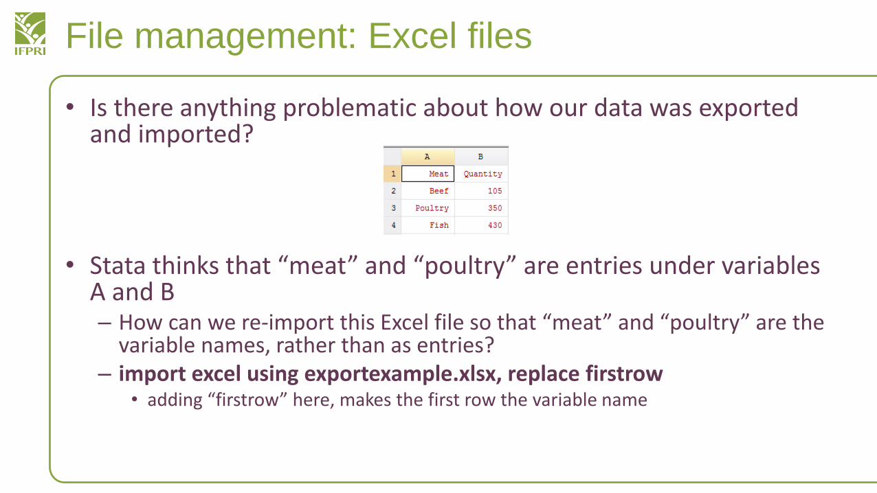
• Is there anything problematic about how our data was exported and imported?

• Stata thinks that “meat” and “poultry” are entries under variables A and B– How can we re-import this Excel file so that “meat” and “poultry” are the

variable names, rather than as entries?– import excel using exportexample.xlsx, replace firstrow

• adding “firstrow” here, makes the first row the variable name

Using Help Functions

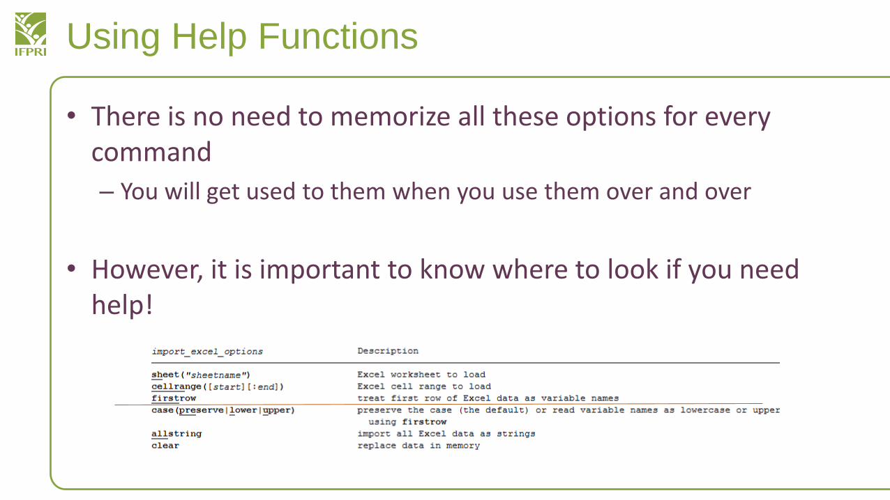
• There is no need to memorize all these options for every command

– You will get used to them when you use them over and over

• However, it is important to know where to look if you need help!


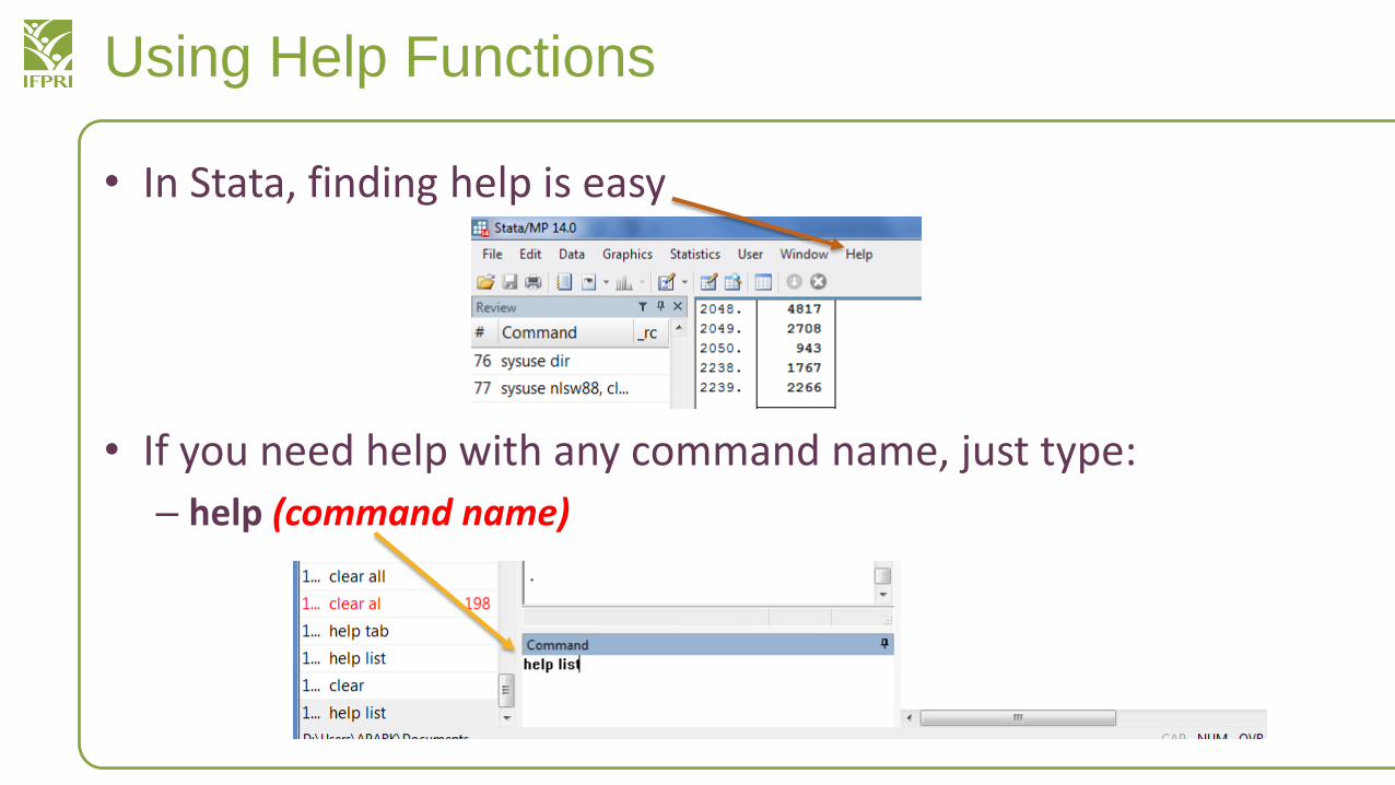
• In Stata, finding help is easy

• If you need help with any command name, just type:

– help (command name)


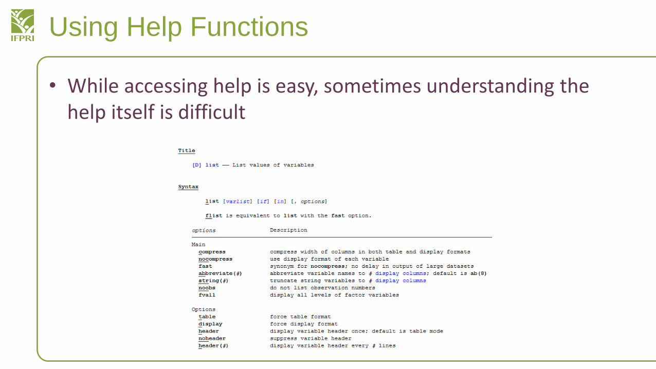
• While accessing help is easy, sometimes understanding the help itself is difficult


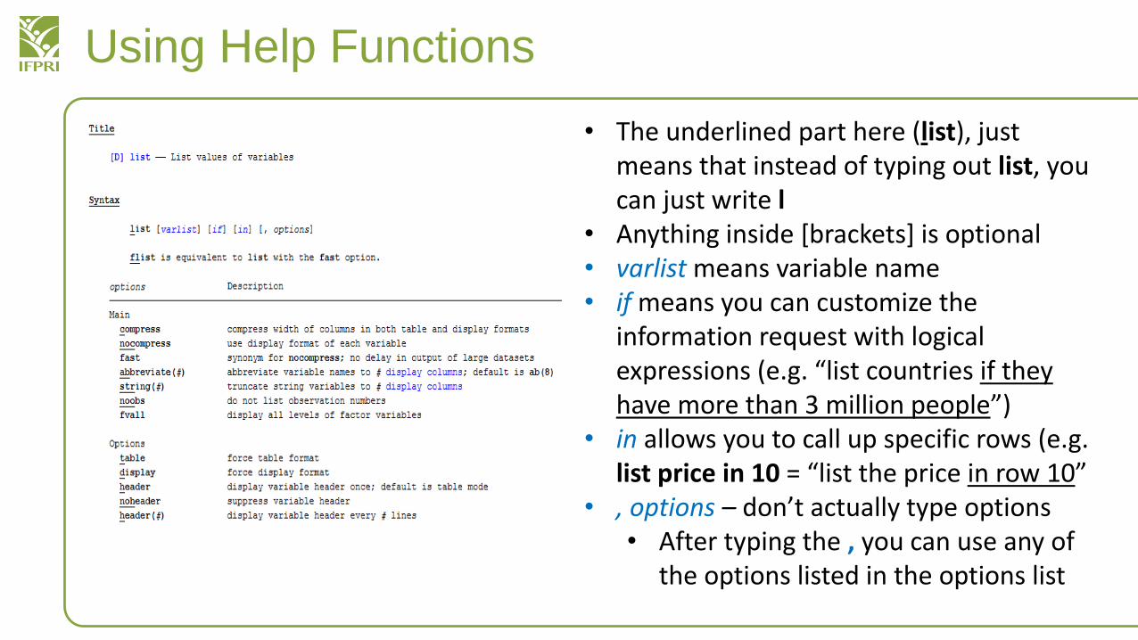
• The underlined part here (list), just means that instead of typing out list, you can just write l

• Anything inside [brackets] is optional• varlist means variable name• if means you can customize the

information request with logical expressions (e.g. “list countries if they have more than 3 million people”)

• in allows you to call up specific rows (e.g. list price in 10 = “list the price in row 10”

• , options – don’t actually type options• After typing the , you can use any of

the options listed in the options list

More Stata Resources

• http://www.stata.com/links

• http://www.stata.com/support

• http://www.ats.ucla.edu/stat/stata – University of California, Los Angeles Stata course (very comprehensive)

• http://data.princeton.edu/stata – Princeton University (more basic)

http://www.stata.com/links

http://www.stata.com/support

http://www.ats.ucla.edu/stat/stata

http://data.princeton.edu/stata

Review: Basic Data Commands

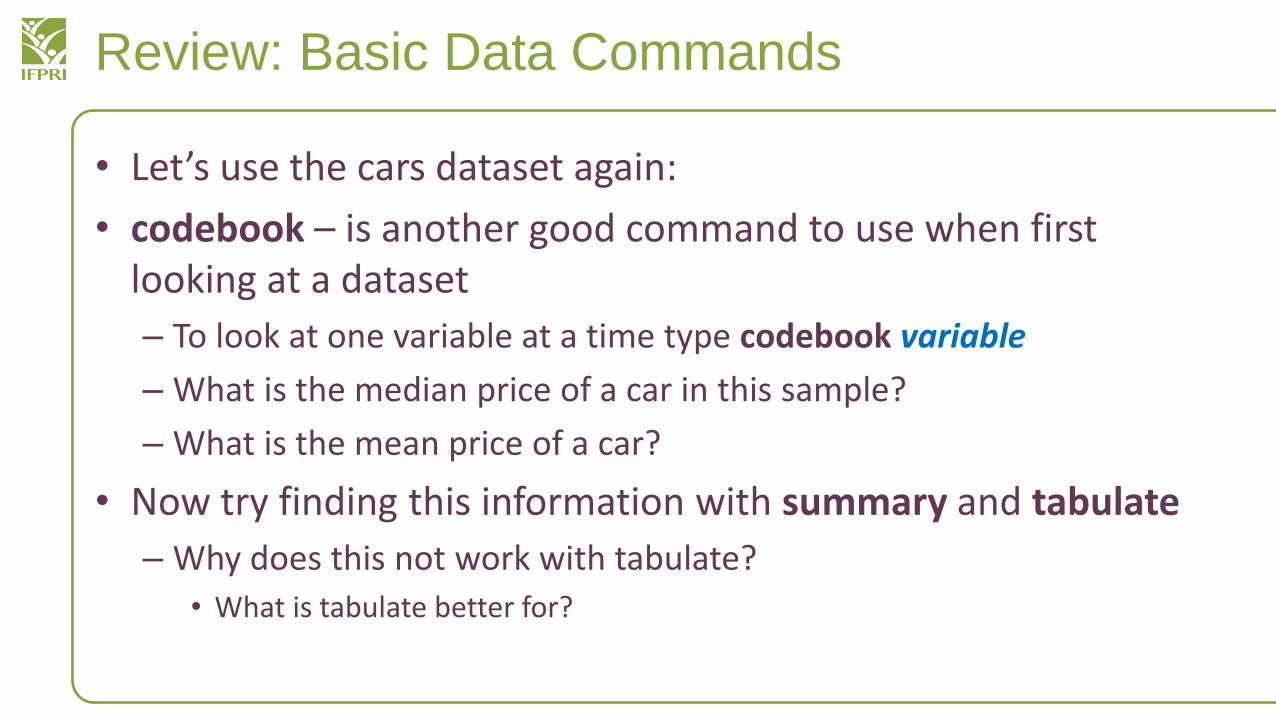
• Let’s use the cars dataset again:

• codebook – is another good command to use when first looking at a dataset

– To look at one variable at a time type codebook variable

– What is the median price of a car in this sample?

– What is the mean price of a car?

• Now try finding this information with summary and tabulate

– Why does this not work with tabulate?

• What is tabulate better for?

Review: Basic Data Commands

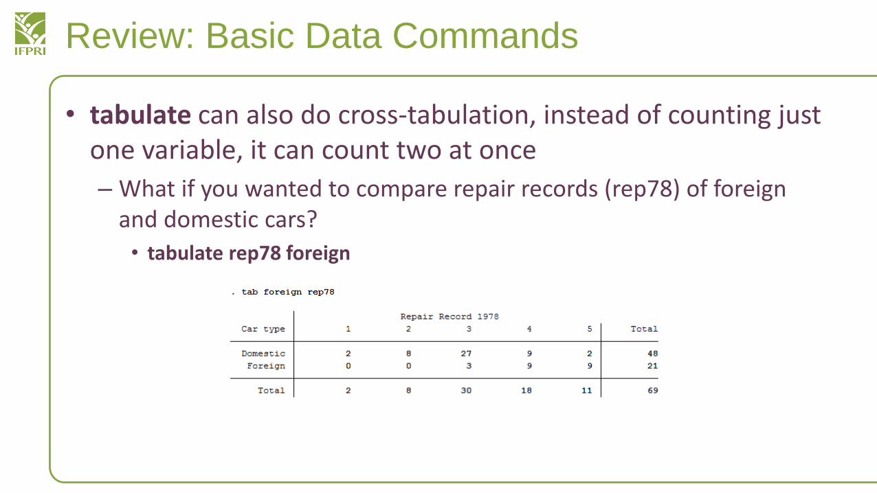
• tabulate can also do cross-tabulation, instead of counting just one variable, it can count two at once

– What if you wanted to compare repair records (rep78) of foreign and domestic cars?

• tabulate rep78 foreign

Variables

• Variables are the basis for most analysis done through Stata

• We have learned how to display information using variables so far

• Now we will work on manipulating variables

• Refresh to the original auto dataset, by sysuse auto, clear

Manipulating Variables: Drop

• drop – used for deleting variables and objects within variables

– Can be used “vertically” and “horizontally”

– How can we drop the foreign variable?

• drop foreign

– Now, drop weight and length

• drop weight length

– What if we wanted to delete all foreign cars? (a “horizontal” delete)

• drop if foreign == 1– Remember in Stata, when you want to say “equal” you need the double = sign

Manipulating Variables: Keep

• Refresh the dataset by typing sysuse auto, clear

• keep – works the same way as drop but in reverse

– Let’s keep only the car’s make, price, and car type

• Keep make price foreign

– How would we keep only domestic cars?

• Keep if foreign == 0– Usually for dummy variables (where the value is 0 or 1), 1 means “yes” and 0 means

“no”

Variables

• Let’s use a different data set this time– sysuse census

• What happened when you tried this?– You need to clear the data first if you are moving between different data sets

» Either use clear and then sysuse census…» Or type sysuse census, clear to do the same thing

• Just for review…– Can you describe the dataset?– Count how many states there are?– What is the average population of the states?– Tabulate the states that are in each region?

• How many states are in the South region?

Manipulating Variables: Generate

• generate – command allows us to create new variables– We want to know the percentage of adult (> 18 years) population for each state

• Generate adultpop = pop18p / pop– What we did was to create the percentage by dividing the population of adults by the total population

• This is why we use == for equal in logical expressions: in Stata the single =is used to assign values to a variable– When we see generate adultpop = pop18p / pop,

• We mean “generate a variable named adultpop whose value will be assigned pop18p divided by pop”

– Be careful of confusing = and ==

– Always remember to specify the name of the variable you want to create after generate!


• Let’s generate a variable named USA that shows “1” for all states that are in the U.S. (hint: all these states are in the U.S.)– generate USA = 1

• This command assigns “1” to every single entry in the variable USA

• Quick review: what is the average adult population in our sample?– sum pop18p

• Can you create a variable named child that shows the total population of children (0-17 years old)– generate child = poplt5 + pop5_17

• Let’s create a new variable named above that shows states that are above the average adult population share, how?– generate above if adultpop > 0.71 (????)

• What’s missing?• We need to assign a value to “above”… otherwise, what would appear in the column?

– The correct syntax is generate above = 1 if adultpop > 0.71• It does not necessary have to be 1, you can really put anything there


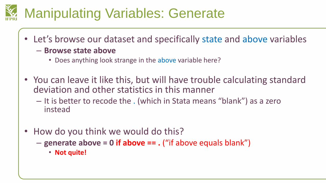
• Let’s browse our dataset and specifically state and above variables– Browse state above

• Does anything look strange in the above variable here?

• You can leave it like this, but will have trouble calculating standard deviation and other statistics in this manner– It is better to recode the . (which in Stata means “blank”) as a zero

instead

• How do you think we would do this?– generate above = 0 if above == . (“if above equals blank”)

• Not quite!

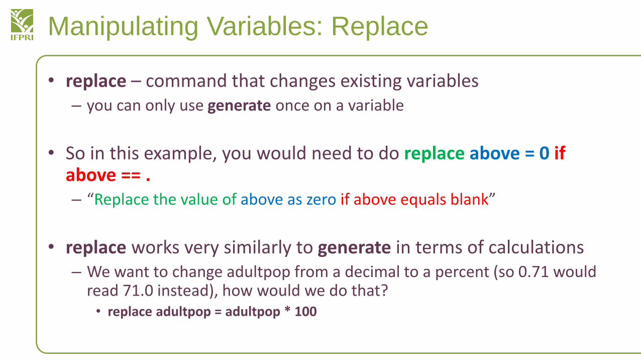
Manipulating Variables: Replace

• replace – command that changes existing variables– you can only use generate once on a variable

• So in this example, you would need to do replace above = 0 if above == .– “Replace the value of above as zero if above equals blank”

• replace works very similarly to generate in terms of calculations– We want to change adultpop from a decimal to a percent (so 0.71 would

read 71.0 instead), how would we do that?• replace adultpop = adultpop * 100

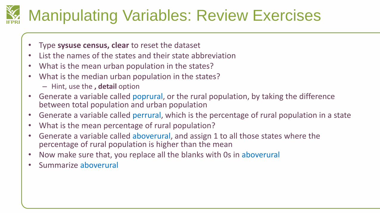
Manipulating Variables: Review Exercises

• Type sysuse census, clear to reset the dataset• List the names of the states and their state abbreviation• What is the mean urban population in the states?• What is the median urban population in the states?

– Hint, use the , detail option

• Generate a variable called poprural, or the rural population, by taking the difference between total population and urban population

• Generate a variable called perrural, which is the percentage of rural population in a state• What is the mean percentage of rural population?• Generate a variable called aboverural, and assign 1 to all those states where the

percentage of rural population is higher than the mean• Now make sure that, you replace all the blanks with 0s in aboverural• Summarize aboverural

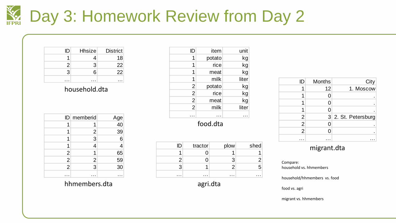
Day 3: Homework Review from Day 2

ID Hhsize District

1 4 18

2 3 22

3 6 22

… … ...

ID memberid Age

1 1 40

1 2 39

1 3 6

1 4 4

2 1 65

2 2 59

2 3 30

… … …

ID item unit

1 potato kg

1 rice kg

1 meat kg

1 milk liter

2 potato kg

2 rice kg

2 meat kg

2 milk liter

… … …

ID tractor plow shed

1 0 1 1

2 0 3 2

3 1 2 5

… … … …

ID Months City

1 12 1. Moscow

1 0 .

1 0 .

1 0 .

2 3 2. St. Petersburg

2 0 .

2 0 .

… … …

household.dta

hhmembers.dta agri.dta

food.dta

migrant.dta

Compare:household vs. hhmembers

household/hhmembers vs. food

food vs. agri

migrant vs. hhmembers

Recoding Variables

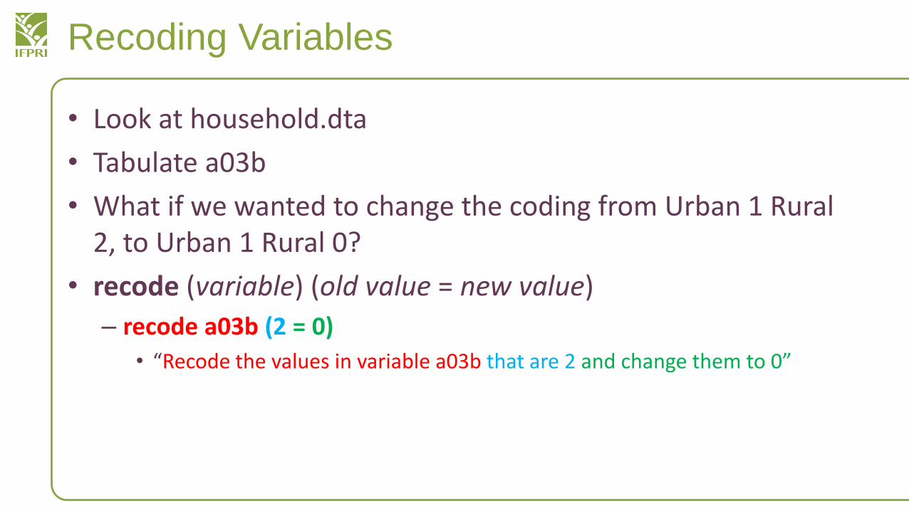
• Look at household.dta

• Tabulate a03b

• What if we wanted to change the coding from Urban 1 Rural 2, to Urban 1 Rural 0?

• recode (variable) (old value = new value)

– recode a03b (2 = 0)

• “Recode the values in variable a03b that are 2 and change them to 0”

Recoding Variables

• After recoding the variables, tabulate them again

• Does anything seem problematic?

– You see “1. Urban and 0”

• After rural was re-coded to 0, the labels didn’t change with it

• You need to also change the label value

Variables Manager

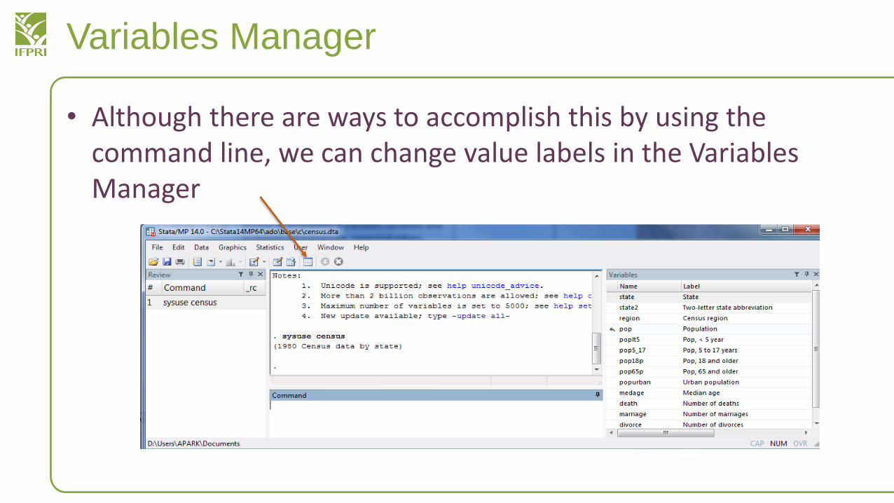
• Although there are ways to accomplish this by using the command line, we can change value labels in the Variables Manager

Variables Manager

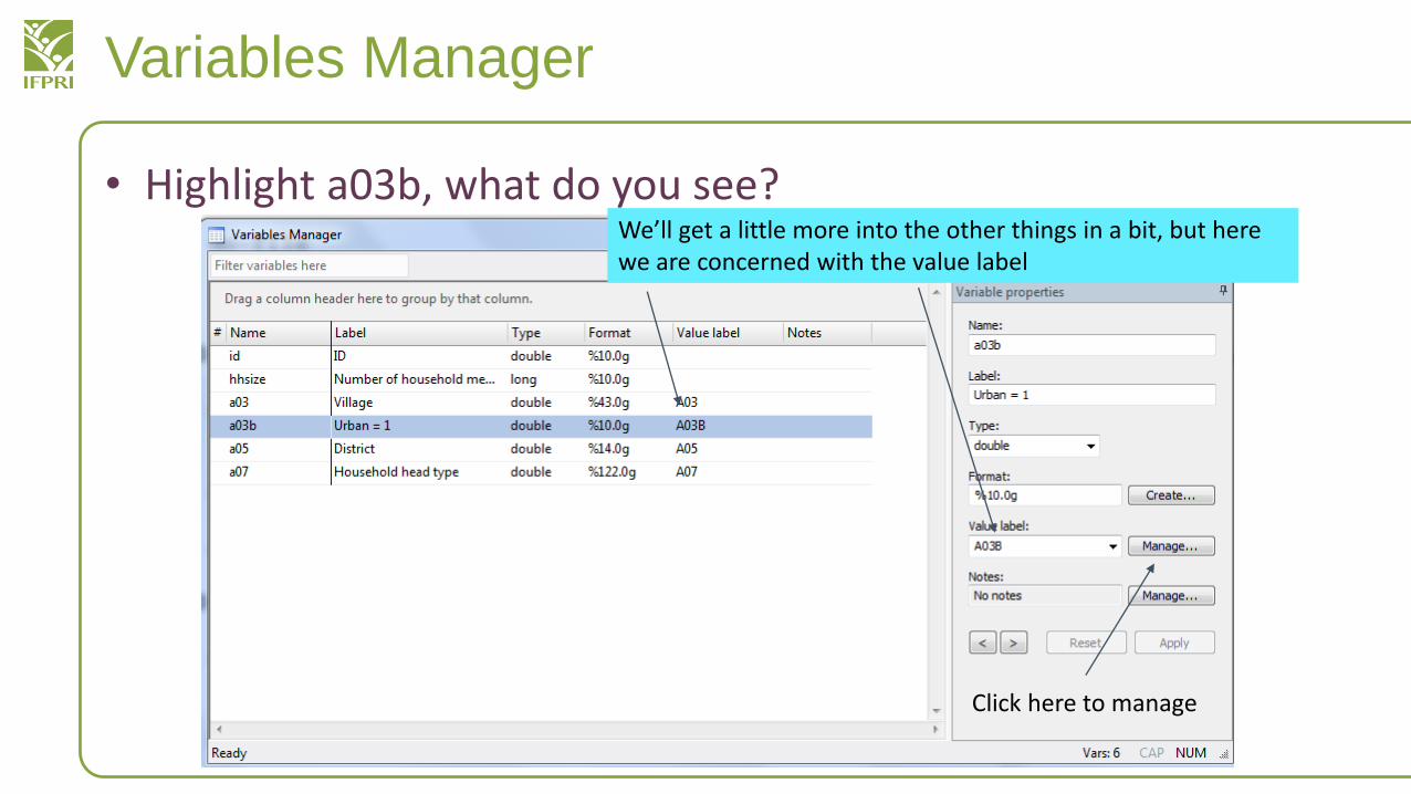
• Highlight a03b, what do you see?We’ll get a little more into the other things in a bit, but here we are concerned with the value label

Click here to manage

Variables Manager

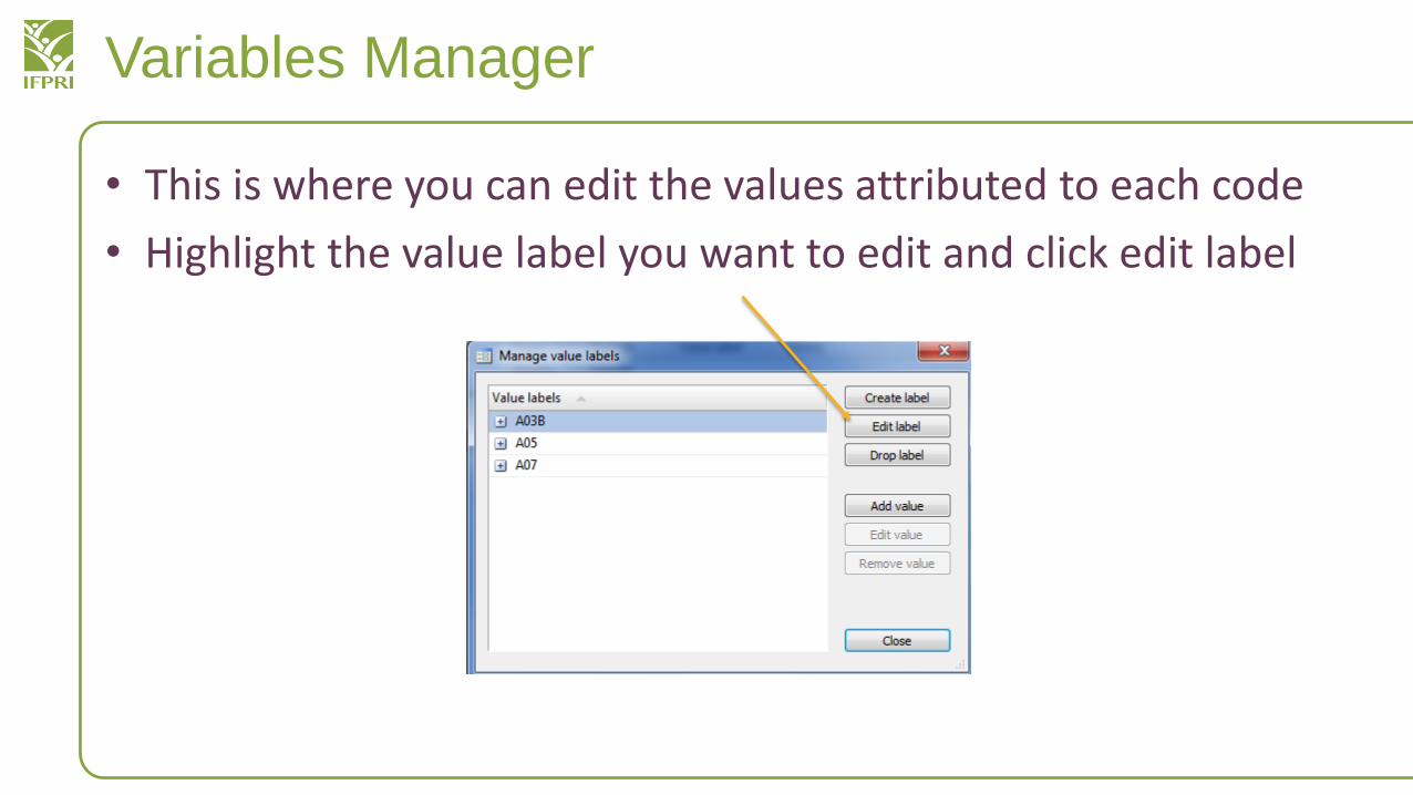
• This is where you can edit the values attributed to each code

• Highlight the value label you want to edit and click edit label

Variables Manager

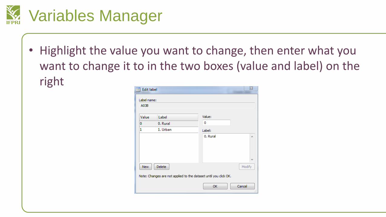
• Highlight the value you want to change, then enter what you want to change it to in the two boxes (value and label) on the right

Variables Manager

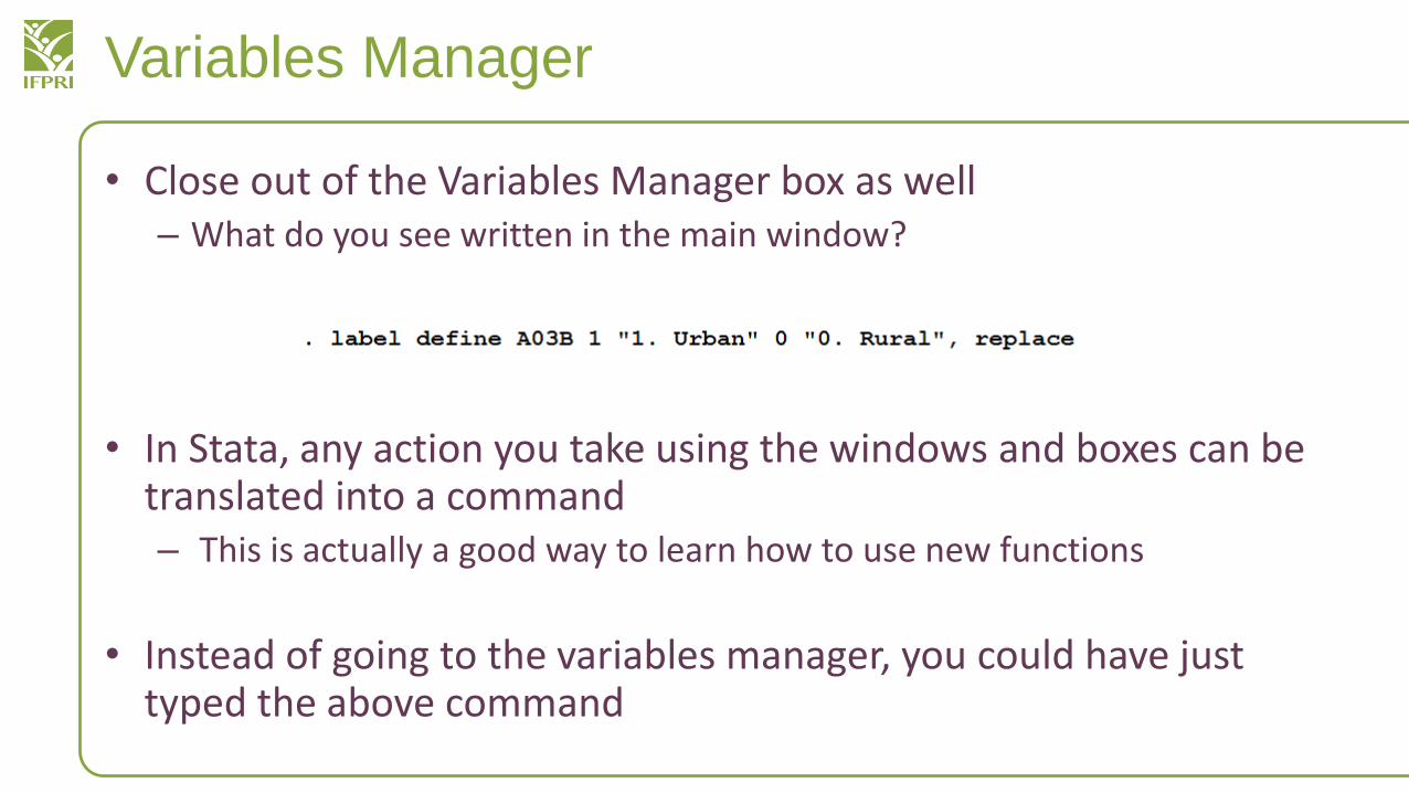
• Close out of the Variables Manager box as well– What do you see written in the main window?

• In Stata, any action you take using the windows and boxes can be translated into a command– This is actually a good way to learn how to use new functions

• Instead of going to the variables manager, you could have just typed the above command

Labeling Variables

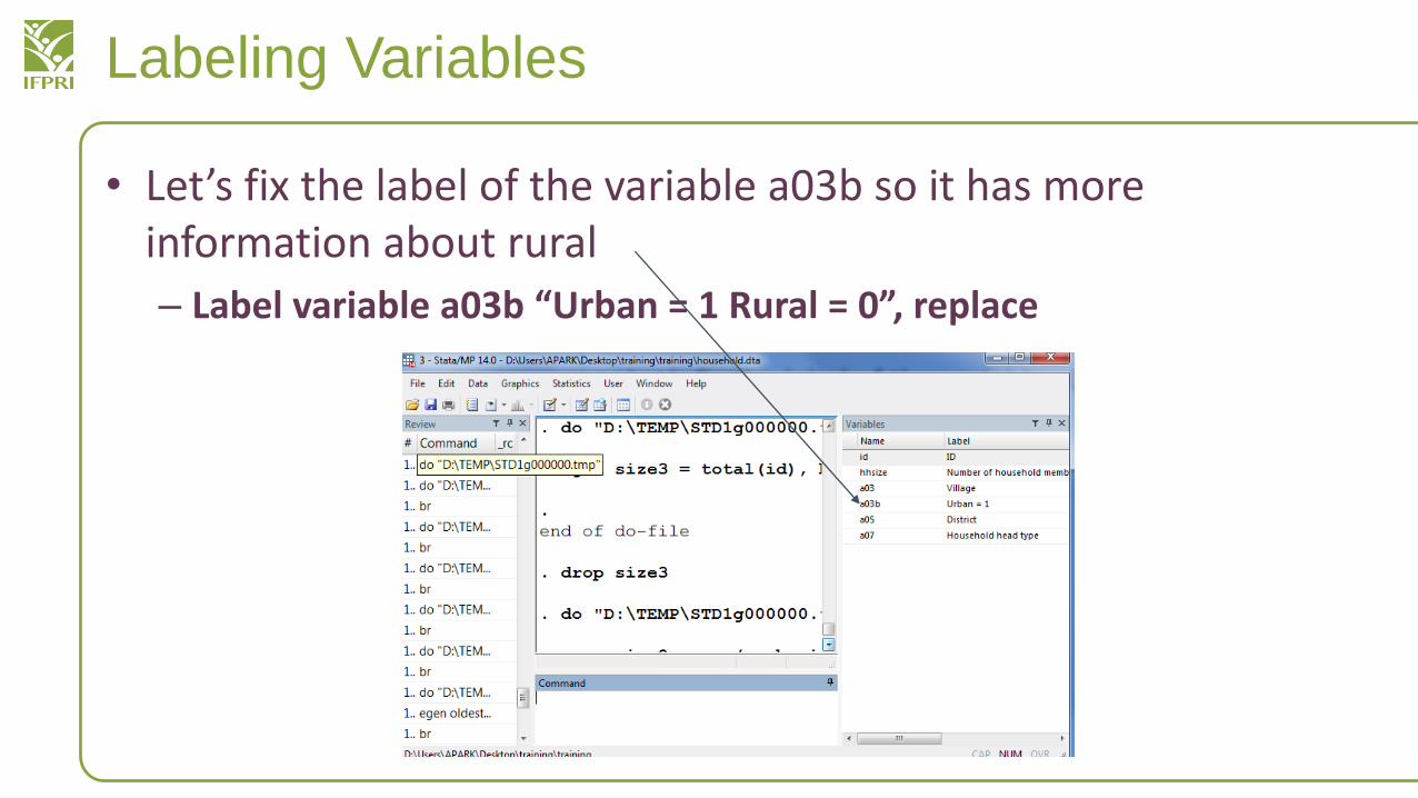
• Let’s fix the label of the variable a03b so it has more information about rural

– Label variable a03b “Urban = 1 Rural = 0”, replace

Renaming variables

• Turn a03b to “urban”

– Use rename a03b urban

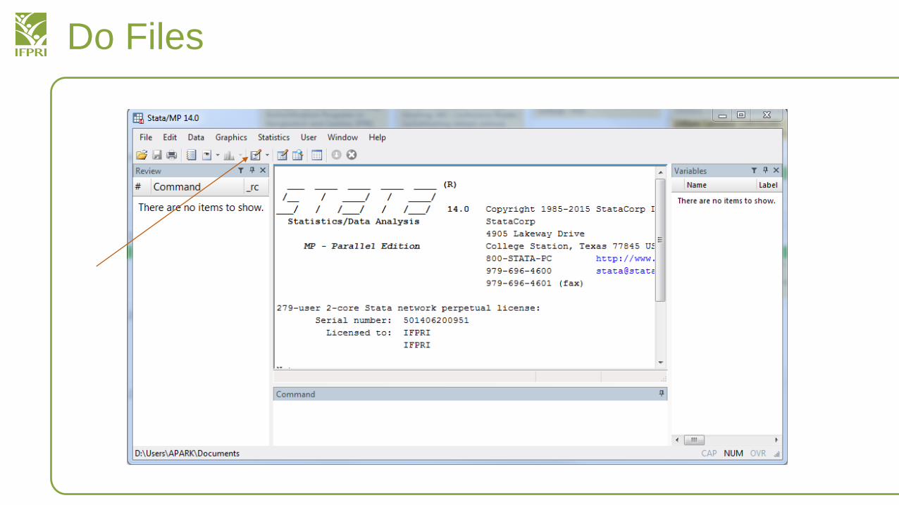
Do Files

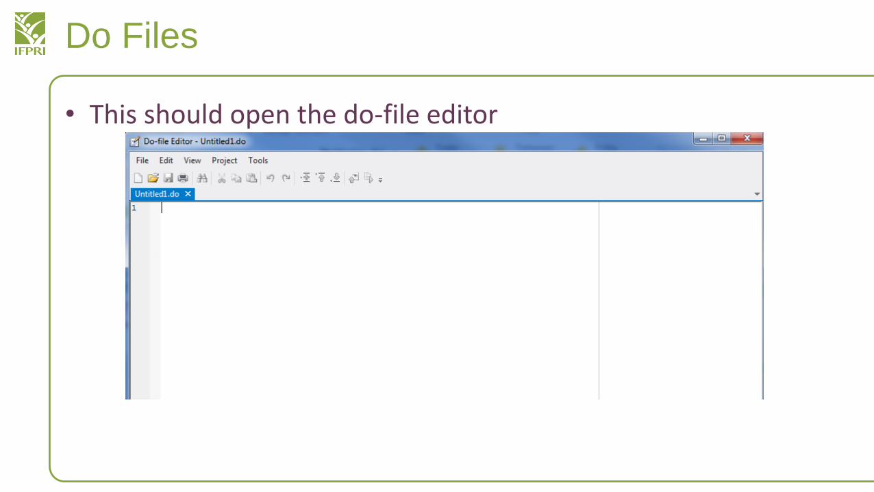
Do Files

• This should open the do-file editor

Do-Files

• Until now, we have been entering commands into the command line only, which is fine

• However, we want to track what we are doing and repeat our steps in the future, it is better to use a do file

– This also helps share your steps with other researchers

• Looking at other do files also is useful in learning Stata

– No need to discover codes yourself, if you can look at existing work by others

Do-Files

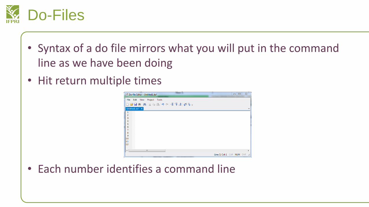
• Syntax of a do file mirrors what you will put in the command line as we have been doing

• Hit return multiple times

• Each number identifies a command line

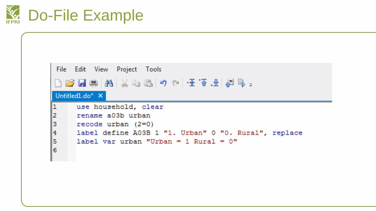
Do-File Example

Do-File Syntax

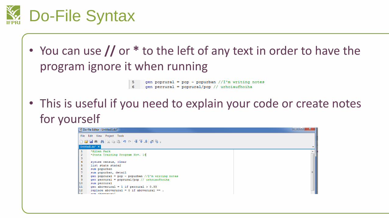
• You can use // or * to the left of any text in order to have the program ignore it when running

• This is useful if you need to explain your code or create notes for yourself

Running Do Files

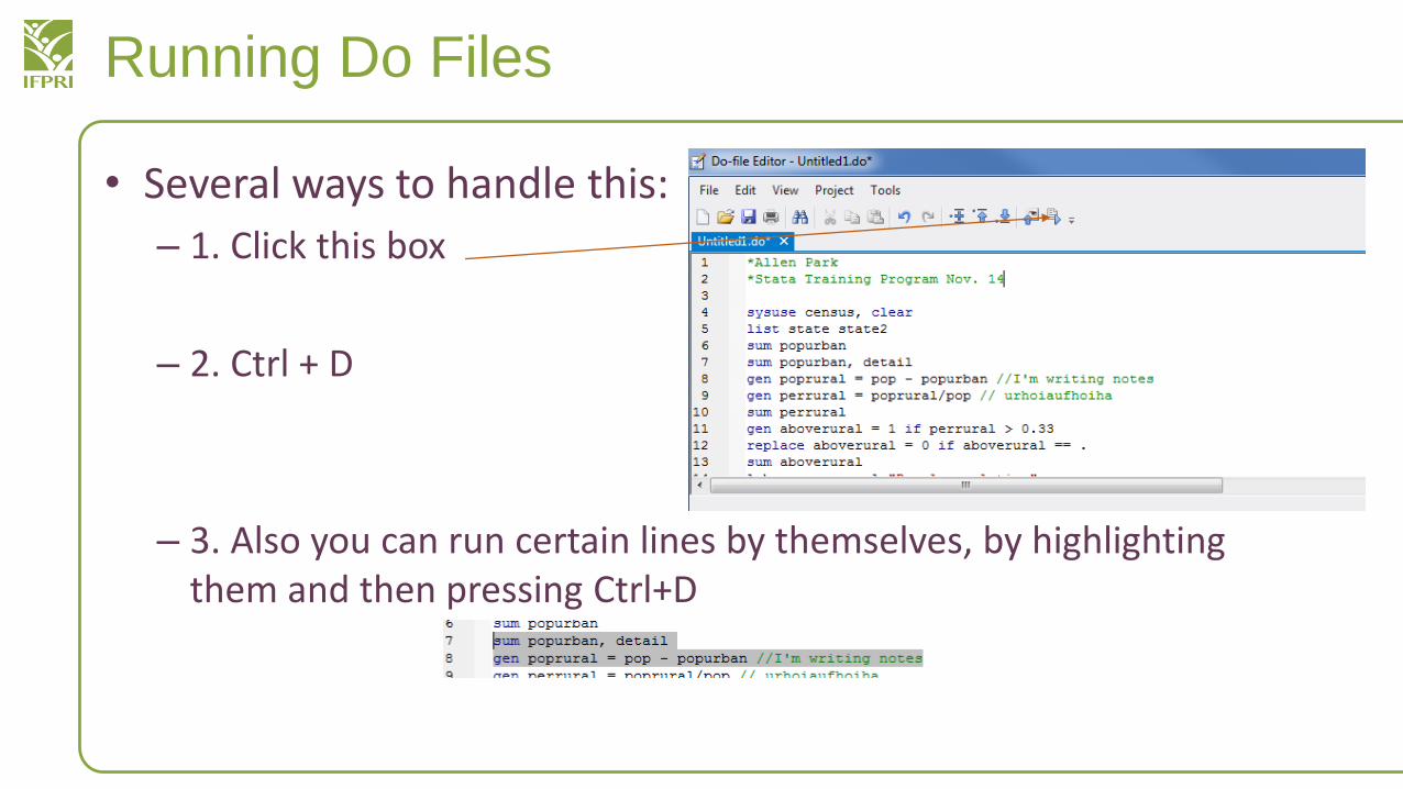
• Several ways to handle this:

– 1. Click this box

– 2. Ctrl + D

– 3. Also you can run certain lines by themselves, by highlighting them and then pressing Ctrl+D

Do File Management

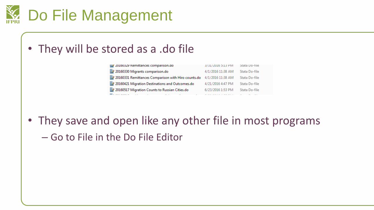
• They will be stored as a .do file

• They save and open like any other file in most programs

– Go to File in the Do File Editor

Log Files

• Do files capture the commands you use to run a dataset

• Log files capture what you see on the screen

• Insert log using training before the start of the do file

• Insert log close at the end of your work to stop capturing

Variables Manager

• For this next section, let’s use the dataset for census

• Tabulate the region variable– Do the names of the regions look strange?

• Ideally we would like these regions to be standardized– NE should be “Northeast” and N Cntrl should be “North Central”

• How can we accomplish this?– What happens when we try to use replace?

• replace region = “Northeast” if region == “NE”

• Why didn’t this work?– It’s because even though we see the different categories as text/words, the actual data has been encoded

as numbers– What we are actually seeing here is the label that has been assigned to each variable

• Type tab region, nolabel– This , nolabel option allows us to see the data without the label that makes us see the data as words

Variables: Storage Type

• Describe the variables in the dataset, how?

• Under “storage type,” you see a number of different options– str2, str14 – these are string variables, text/words/numbers that act as

non-mathematical data, the number to the right shows how many characters are allowed there

– int – this is integer data

– float – this is numerical data that can have many decimal places

– long – the same idea as float, but not as many spaces

• Why is this important?– Each variable can only be one type at a time; you cannot have string data

and integer data in the same variable, etc.

Appending and Merging

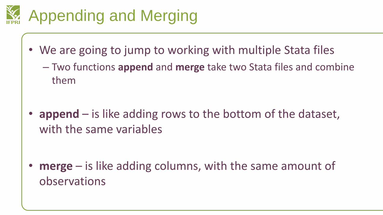
• We are going to jump to working with multiple Stata files

– Two functions append and merge take two Stata files and combine them

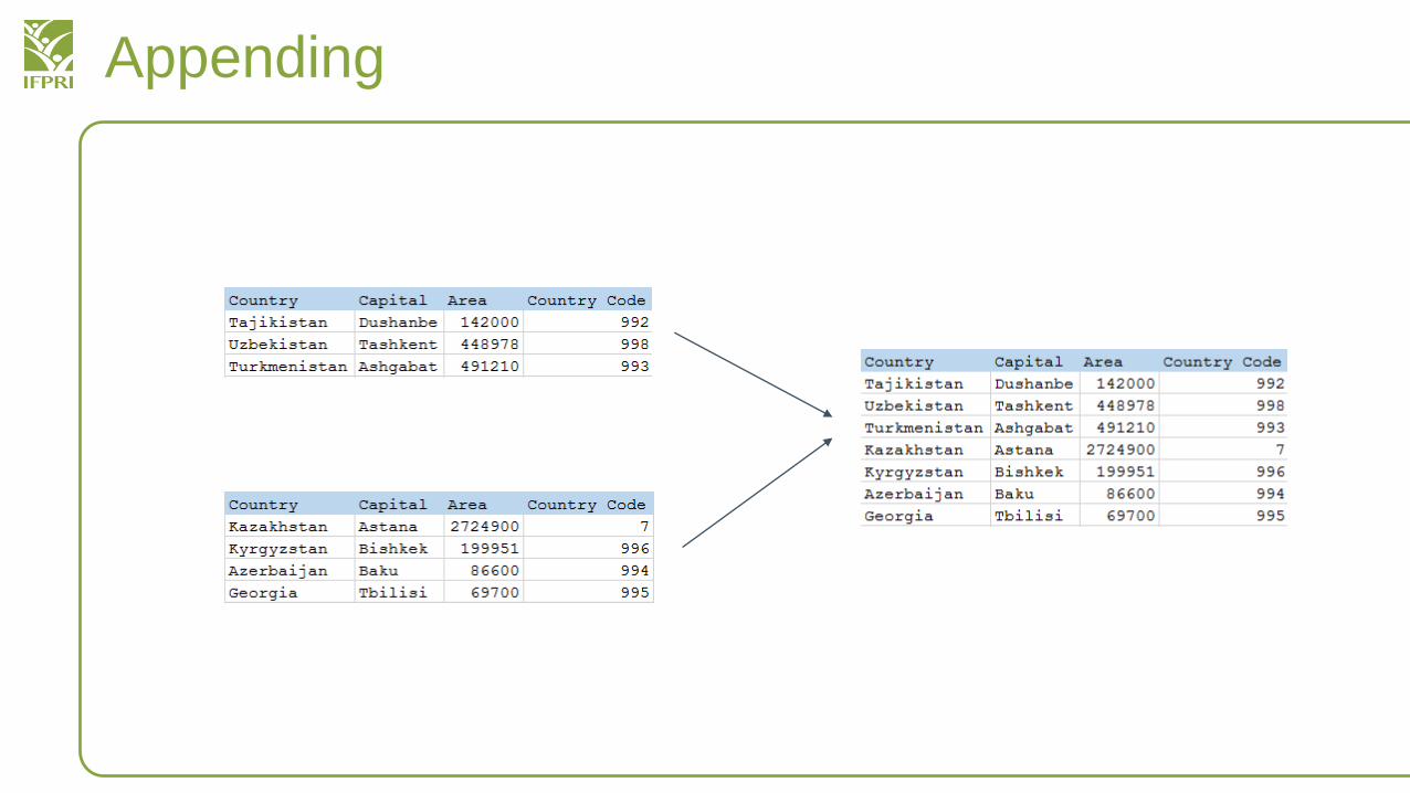
• append – is like adding rows to the bottom of the dataset, with the same variables

• merge – is like adding columns, with the same amount of observations

Appending

Appending

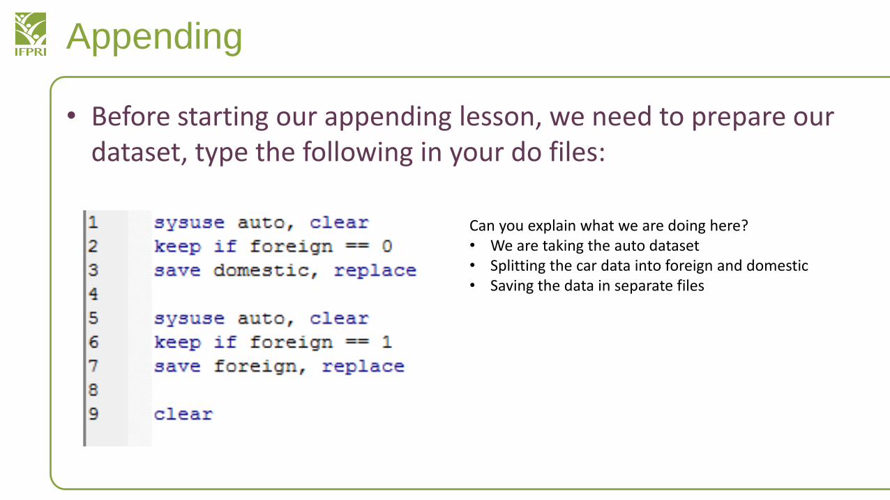
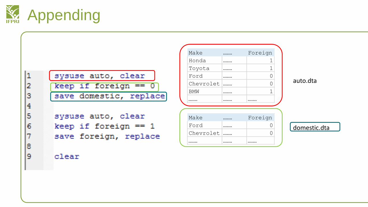
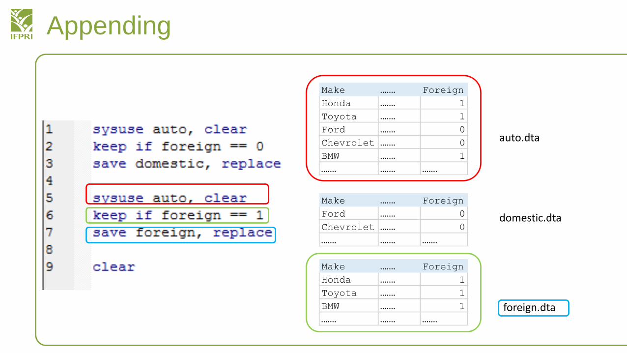
• Before starting our appending lesson, we need to prepare our dataset, type the following in your do files:

Can you explain what we are doing here?• We are taking the auto dataset • Splitting the car data into foreign and domestic• Saving the data in separate files

Appending

Make ……. Foreign

Honda ……. 1

Toyota ……. 1

Ford ……. 0

Chevrolet ……. 0

BMW ……. 1

……. ……. …….


Ford ……. 0

Chevrolet ……. 0

……. ……. …….

auto.dta

domestic.dta

Appending


Honda ……. 1

Toyota ……. 1

Ford ……. 0

Chevrolet ……. 0

BMW ……. 1

……. ……. …….


Ford ……. 0

Chevrolet ……. 0

……. ……. …….

auto.dta

domestic.dta


Honda ……. 1

Toyota ……. 1

BMW ……. 1

……. ……. …….foreign.dta

Appending

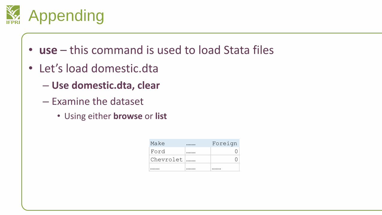
• use – this command is used to load Stata files

• Let’s load domestic.dta

– Use domestic.dta, clear

– Examine the dataset

• Using either browse or list


Ford ……. 0

Chevrolet ……. 0

……. ……. …….

Appending

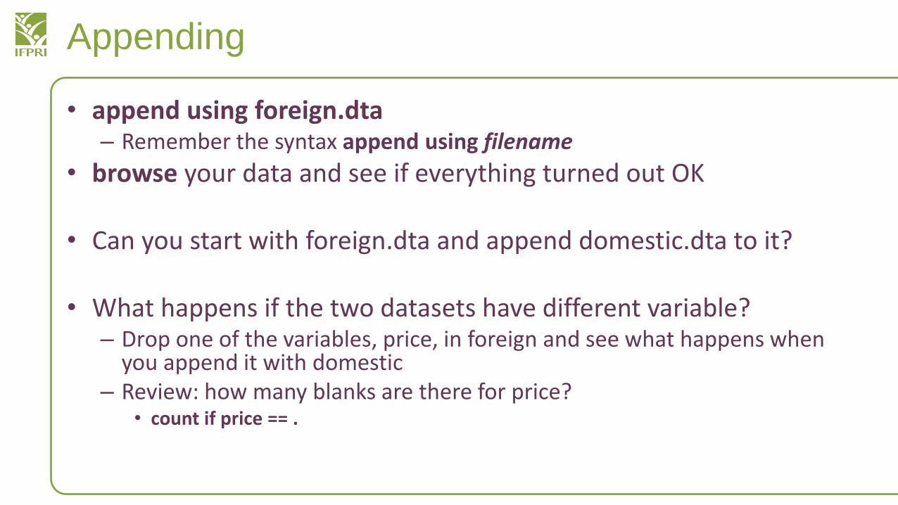
• append using foreign.dta– Remember the syntax append using filename

• browse your data and see if everything turned out OK

• Can you start with foreign.dta and append domestic.dta to it?

• What happens if the two datasets have different variable?– Drop one of the variables, price, in foreign and see what happens when

you append it with domestic– Review: how many blanks are there for price?

• count if price == .

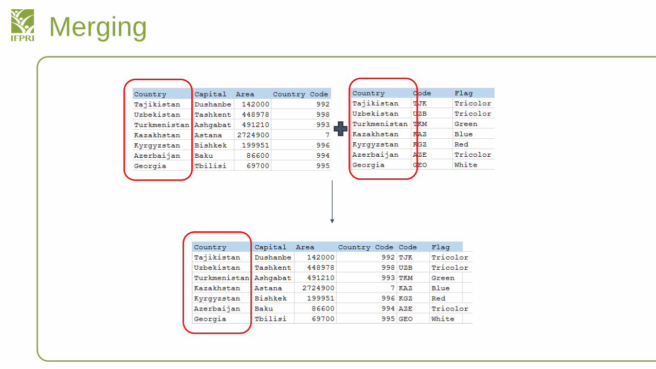
Merging

Merge

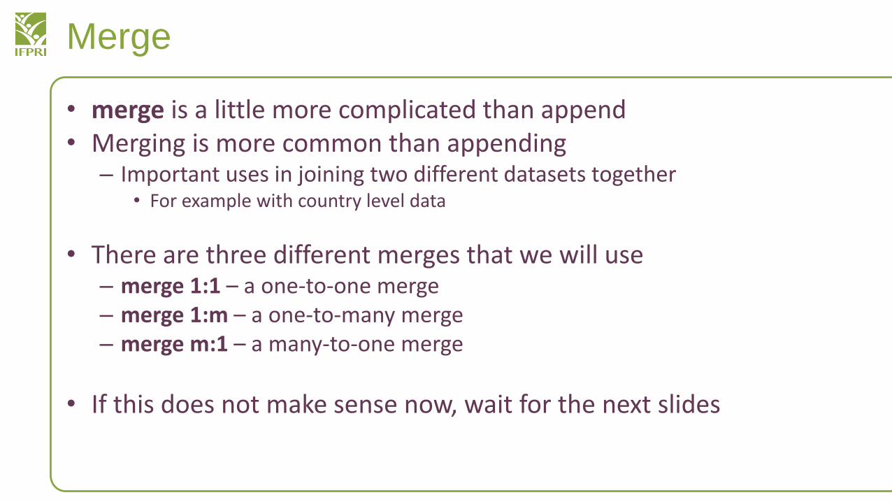
• merge is a little more complicated than append• Merging is more common than appending

– Important uses in joining two different datasets together• For example with country level data

• There are three different merges that we will use– merge 1:1 – a one-to-one merge– merge 1:m – a one-to-many merge– merge m:1 – a many-to-one merge

• If this does not make sense now, wait for the next slides

Merge 1:1

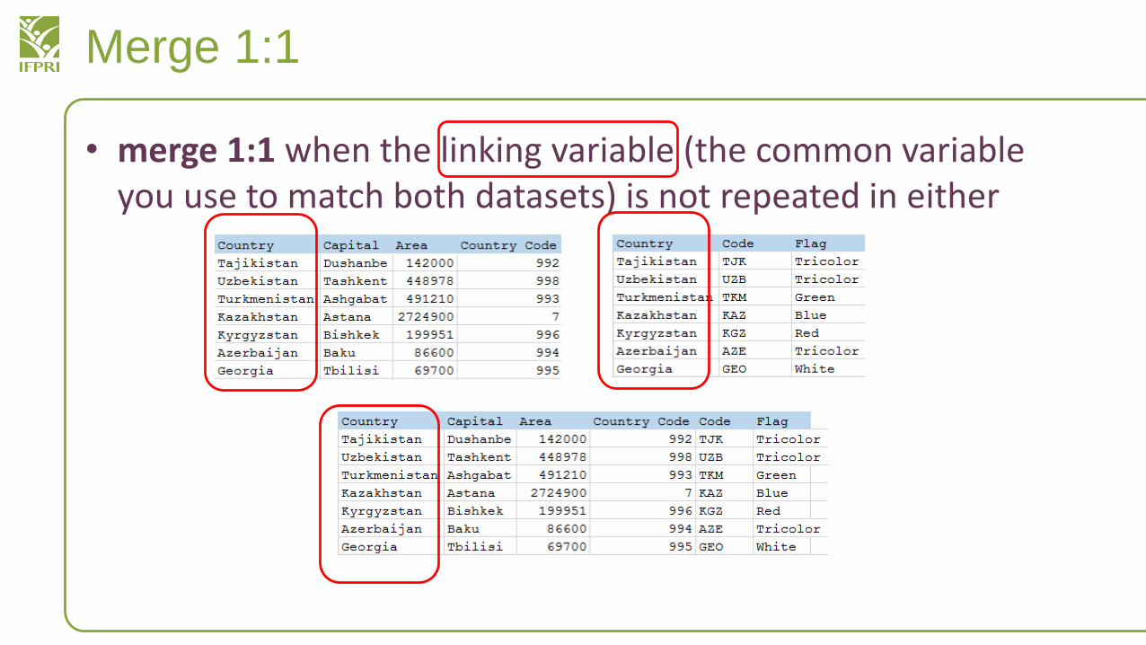
• merge 1:1 when the linking variable (the common variable you use to match both datasets) is not repeated in either

Detecting Duplicates

• duplicates list (variable name)

– If we want to see if there are any ID numbers that are repeated in a dataset we would use duplicates list id

• If you are doing a 1:1 merge, you need to make sure that there are no repeats in the linking variable

– You can have repeats in other variables but not the linking variable

Merge 1:m

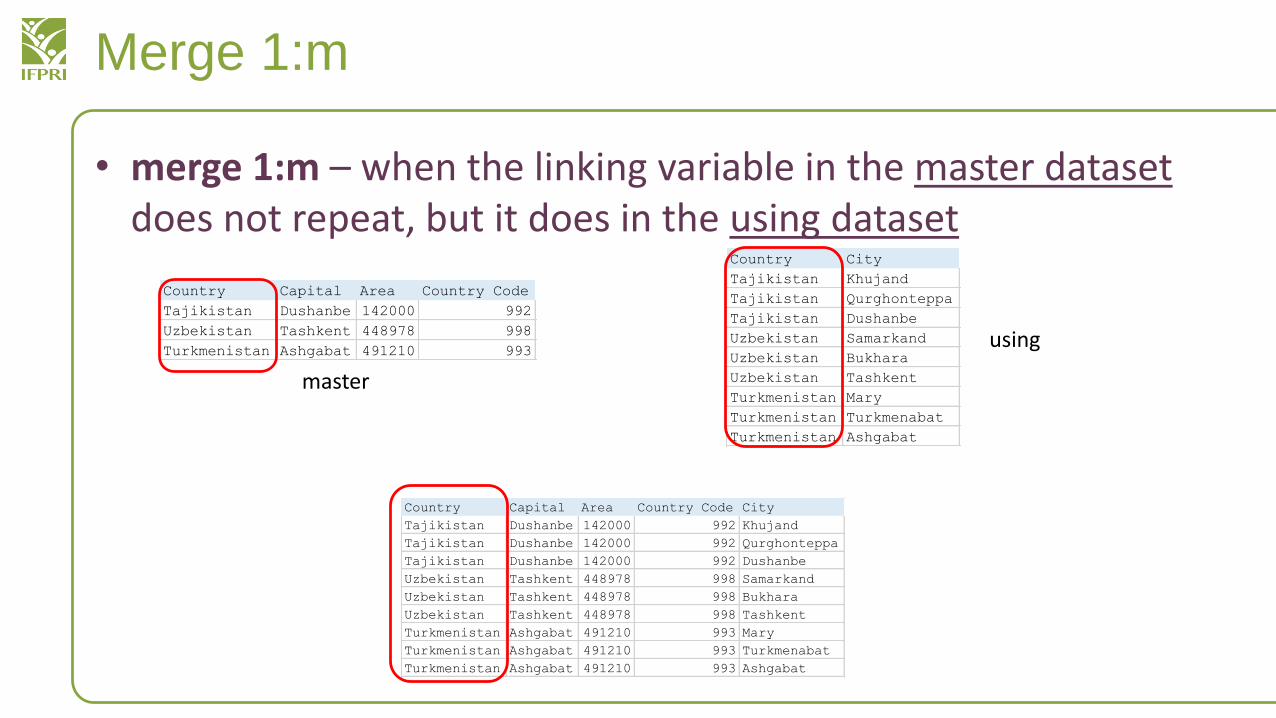
• merge 1:m – when the linking variable in the master dataset does not repeat, but it does in the using dataset

Country Capital Area Country Code

Tajikistan Dushanbe 142000 992

Uzbekistan Tashkent 448978 998

Turkmenistan Ashgabat 491210 993

master

Country City

Tajikistan Khujand

Tajikistan Qurghonteppa

Tajikistan Dushanbe

Uzbekistan Samarkand

Uzbekistan Bukhara

Uzbekistan Tashkent

Turkmenistan Mary

Turkmenistan Turkmenabat

Turkmenistan Ashgabat

using

Country Capital Area Country Code City

Tajikistan Dushanbe 142000 992 Khujand

Tajikistan Dushanbe 142000 992 Qurghonteppa

Tajikistan Dushanbe 142000 992 Dushanbe

Uzbekistan Tashkent 448978 998 Samarkand

Uzbekistan Tashkent 448978 998 Bukhara

Uzbekistan Tashkent 448978 998 Tashkent

Turkmenistan Ashgabat 491210 993 Mary

Turkmenistan Ashgabat 491210 993 Turkmenabat

Turkmenistan Ashgabat 491210 993 Ashgabat

Merge m:1

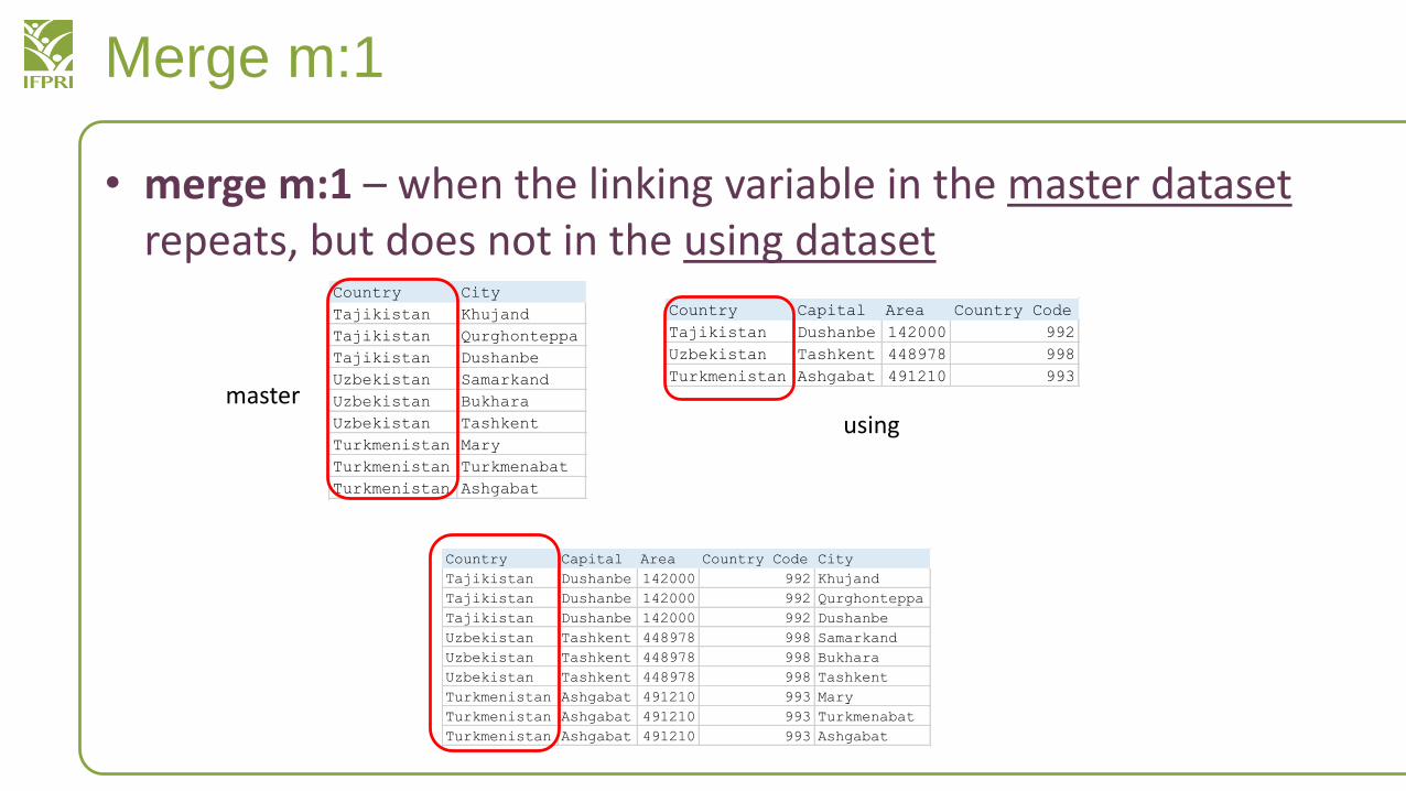
• merge m:1 – when the linking variable in the master dataset repeats, but does not in the using dataset





master

Country City

Tajikistan Khujand


Tajikistan Dushanbe


Uzbekistan Bukhara

Uzbekistan Tashkent

Turkmenistan Mary



using











Merge 1:1

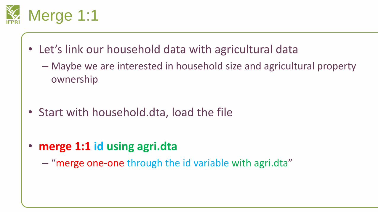
• Let’s link our household data with agricultural data

– Maybe we are interested in household size and agricultural property ownership

• Start with household.dta, load the file

• merge 1:1 id using agri.dta

– “merge one-one through the id variable with agri.dta”

Merge 1:1

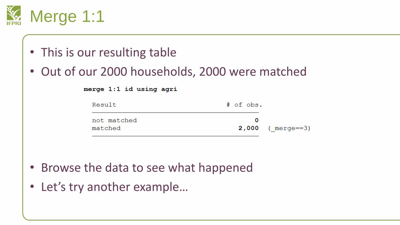
• This is our resulting table

• Out of our 2000 households, 2000 were matched

• Browse the data to see what happened

• Let’s try another example…

Merge 1:1

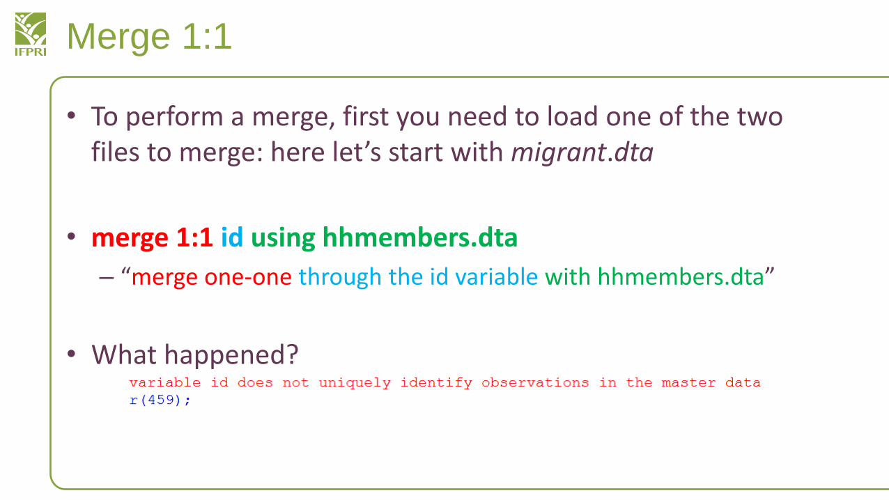
• To perform a merge, first you need to load one of the two files to merge: here let’s start with migrant.dta

• merge 1:1 id using hhmembers.dta

– “merge one-one through the id variable with hhmembers.dta”

• What happened?

Merge 1:1

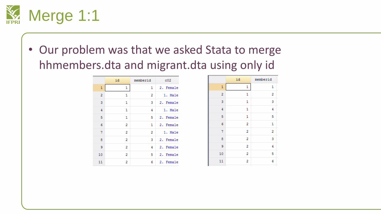
• Our problem was that we asked Stata to merge hhmembers.dta and migrant.dta using only id

Merge 1:1

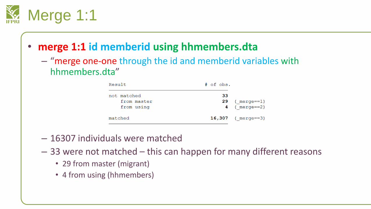
• merge 1:1 id memberid using hhmembers.dta– “merge one-one through the id and memberid variables with

hhmembers.dta”

– 16307 individuals were matched

– 33 were not matched – this can happen for many different reasons• 29 from master (migrant)

• 4 from using (hhmembers)

Merge 1:1

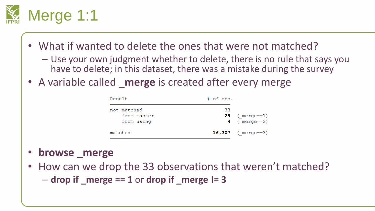
• What if wanted to delete the ones that were not matched?– Use your own judgment whether to delete, there is no rule that says you

have to delete; in this dataset, there was a mistake during the survey

• A variable called _merge is created after every merge

• browse _merge• How can we drop the 33 observations that weren’t matched?

– drop if _merge == 1 or drop if _merge != 3

Merge 1:m

• merge 1:m – when the linking variable in the master dataset does not repeat, but it does in the using dataset





master

Country City

Tajikistan Khujand


Tajikistan Dushanbe


Uzbekistan Bukhara

Uzbekistan Tashkent

Turkmenistan Mary



using











Merge 1:m

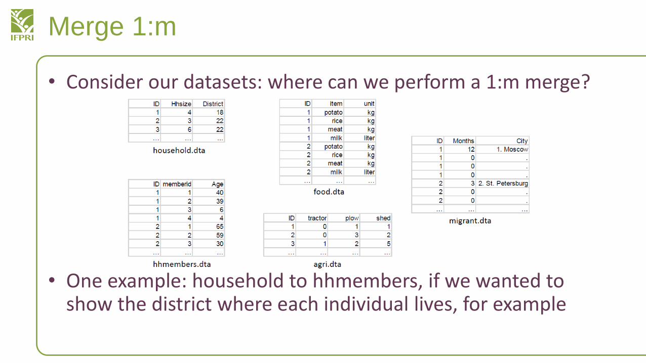
• Consider our datasets: where can we perform a 1:m merge?

• One example: household to hhmembers, if we wanted to show the district where each individual lives, for example

Merge 1:m

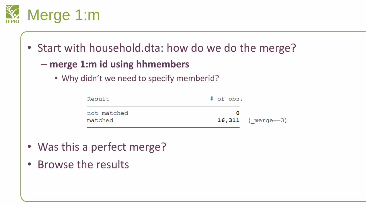
• Start with household.dta: how do we do the merge?

– merge 1:m id using hhmembers

• Why didn’t we need to specify memberid?

• Was this a perfect merge?

• Browse the results

Merge m:1

• merge m:1 – when the linking variable in the master dataset repeats, but does not in the using dataset





master

Country City

Tajikistan Khujand


Tajikistan Dushanbe


Uzbekistan Bukhara

Uzbekistan Tashkent

Turkmenistan Mary



using











Merge: Review Exercise #2

• Load uslifeexp and then load uslifeexp2– Browse them first and examine the data

– Is there a linking variable that is common to both?

– What kind of merge can we do here?

– How can you do it?• merge 1:1 year using uslifeexp2 (if uslifeexp is your master file)

• merge 1:1 year using uslifeexp (if uslifeexp2 is your master file)

– What does the output say?• How many were matched?

• How many were not matched? From which file?– How can we delete the years that were not matched?

Advanced Variable Functions: egen

• egen – “extensions to generate”– Allows you to generate new variables but more advanced showing

you all kinds of data

• Use hhmembers.dta

• egen oldestage = max(c04)– “e-generate a variable called oldestage which is the maximum of

c04 (age)”

• Other options besides max(): min(), median(), mean(), total(), count()


• Can you e-generate a variable called averageage, which is the average age of the sample?

– egen average = mean(c04)

• Can you e-generate a variable called medianage, which is the median age of the sample?

– egen medianage = median(c04)


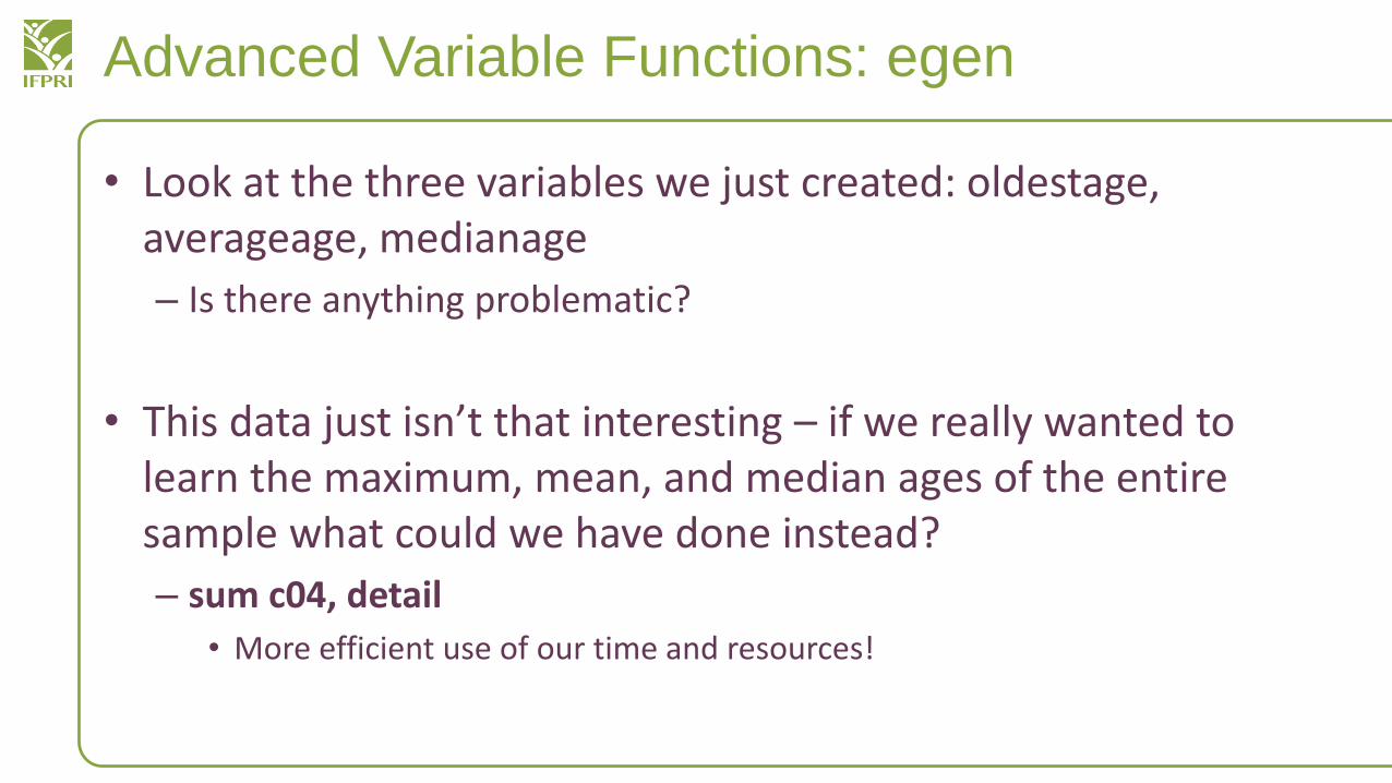
• Look at the three variables we just created: oldestage, averageage, medianage

– Is there anything problematic?

• This data just isn’t that interesting – if we really wanted to learn the maximum, mean, and median ages of the entire sample what could we have done instead?

– sum c04, detail

• More efficient use of our time and resources!


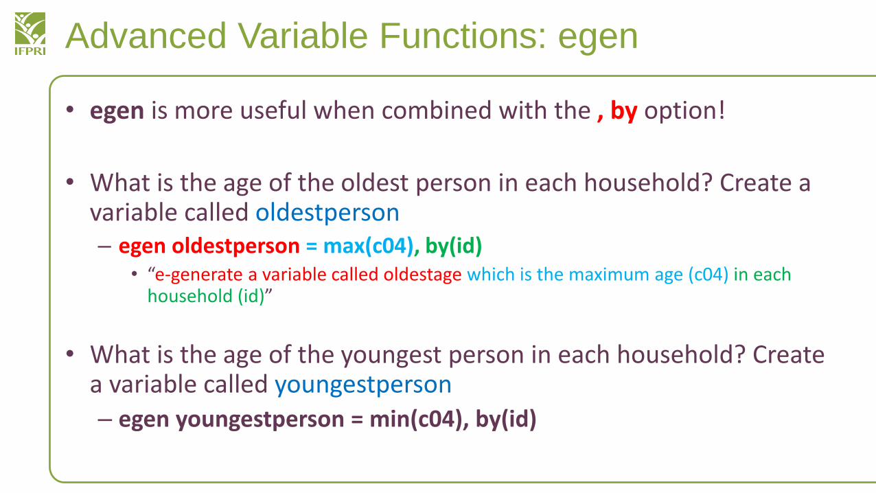
• egen is more useful when combined with the , by option!

• What is the age of the oldest person in each household? Create a variable called oldestperson– egen oldestperson = max(c04), by(id)

• “e-generate a variable called oldestage which is the maximum age (c04) in each household (id)”

• What is the age of the youngest person in each household? Create a variable called youngestperson– egen youngestperson = min(c04), by(id)


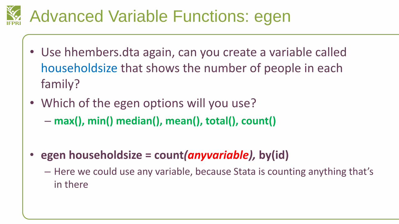
• Use hhembers.dta again, can you create a variable called householdsize that shows the number of people in each family?

• Which of the egen options will you use?

– max(), min() median(), mean(), total(), count()

• egen householdsize = count(anyvariable), by(id)

– Here we could use any variable, because Stata is counting anything that’s in there

Day 4: Review and Preview

• We learned merging and egen yesterday

– Today we will learn how to collapse and reshape data

• Graphing and analysis

Variables: Changing order of a variable

• order [variable name] , after(variable)

• order [variable name] , before(variable)

Variables: Wildcard Functions

• For this slide, let’s use household.dta

• Let’s say we wanted to list only variables who start with the letter a, how would we do that?– * “wildcard” function

• So a* would mean “anything that starts with a”– a03, a05, etc.

– list a*

• What if we wanted to keep only variables that start with a?– Keep a*

Variables: Calling Multiple Variables

• What if we want to keep only hhsize, a03, and a03b

• We can do keep hhsize a03 a03b

• We can also just use keep hhsize – a03b

– This is more useful for datasets with many variables

Review of Merge

• Working in small groups:

• What is the average age of migrants?

• How many women and how many men migrated?

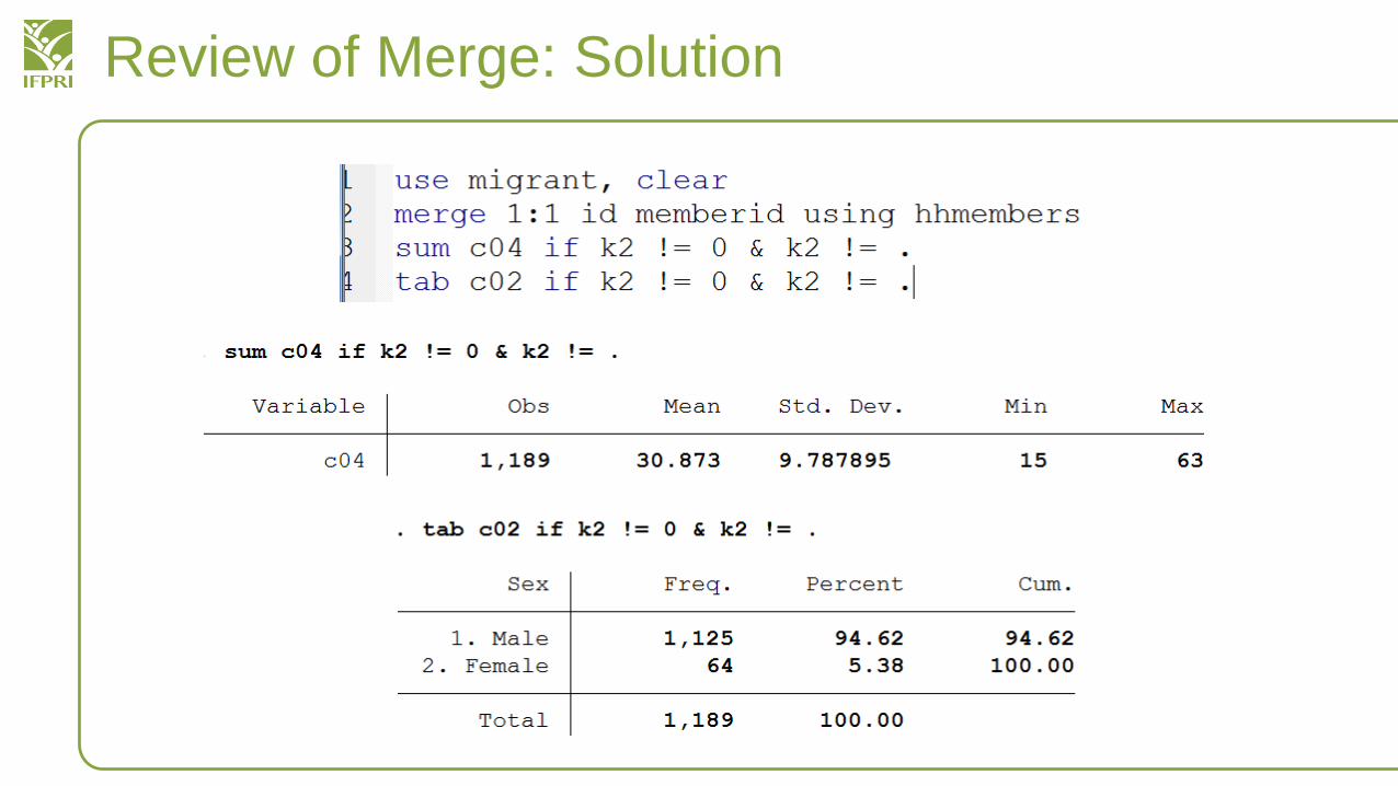
Review of Merge: Solution

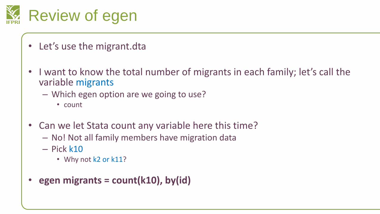
Review of egen

• Let’s use the migrant.dta

• I want to know the total number of migrants in each family; let’s call the variable migrants– Which egen option are we going to use?

• count

• Can we let Stata count any variable here this time?– No! Not all family members have migration data– Pick k10

• Why not k2 or k11?

• egen migrants = count(k10), by(id)

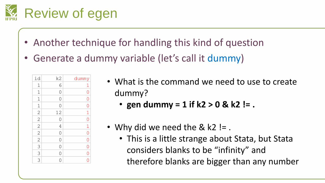
Review of egen

• Another technique for handling this kind of question

• Generate a dummy variable (let’s call it dummy)

id k2 dummy

1 6 1

1 0 0

1 0 0

1 0 0

2 12 1

2 0 0

2 4 1

2 0 0

2 0 0

3 0 0

3 0 0

3 0 0

• What is the command we need to use to create dummy?• gen dummy = 1 if k2 > 0 & k2 != .

• Why did we need the & k2 != .• This is a little strange about Stata, but Stata

considers blanks to be “infinity” and therefore blanks are bigger than any number

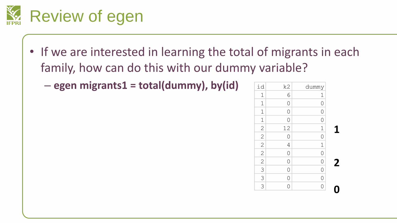
Review of egen

• If we are interested in learning the total of migrants in each family, how can do this with our dummy variable?

– egen migrants1 = total(dummy), by(id) id k2 dummy

1 6 1

1 0 0

1 0 0

1 0 0

2 12 1

2 0 0

2 4 1

2 0 0

2 0 0

3 0 0

3 0 0

3 0 0

1

2

0

Review of egen

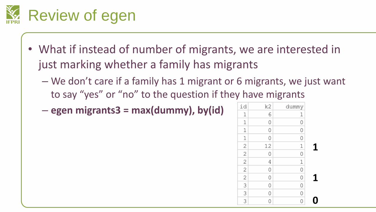
• What if instead of number of migrants, we are interested in just marking whether a family has migrants

– We don’t care if a family has 1 migrant or 6 migrants, we just want to say “yes” or “no” to the question if they have migrants

– egen migrants3 = max(dummy), by(id) id k2 dummy

1 6 1

1 0 0

1 0 0

1 0 0

2 12 1

2 0 0

2 4 1

2 0 0

2 0 0

3 0 0

3 0 0

3 0 0

1

1

0

Review of egen

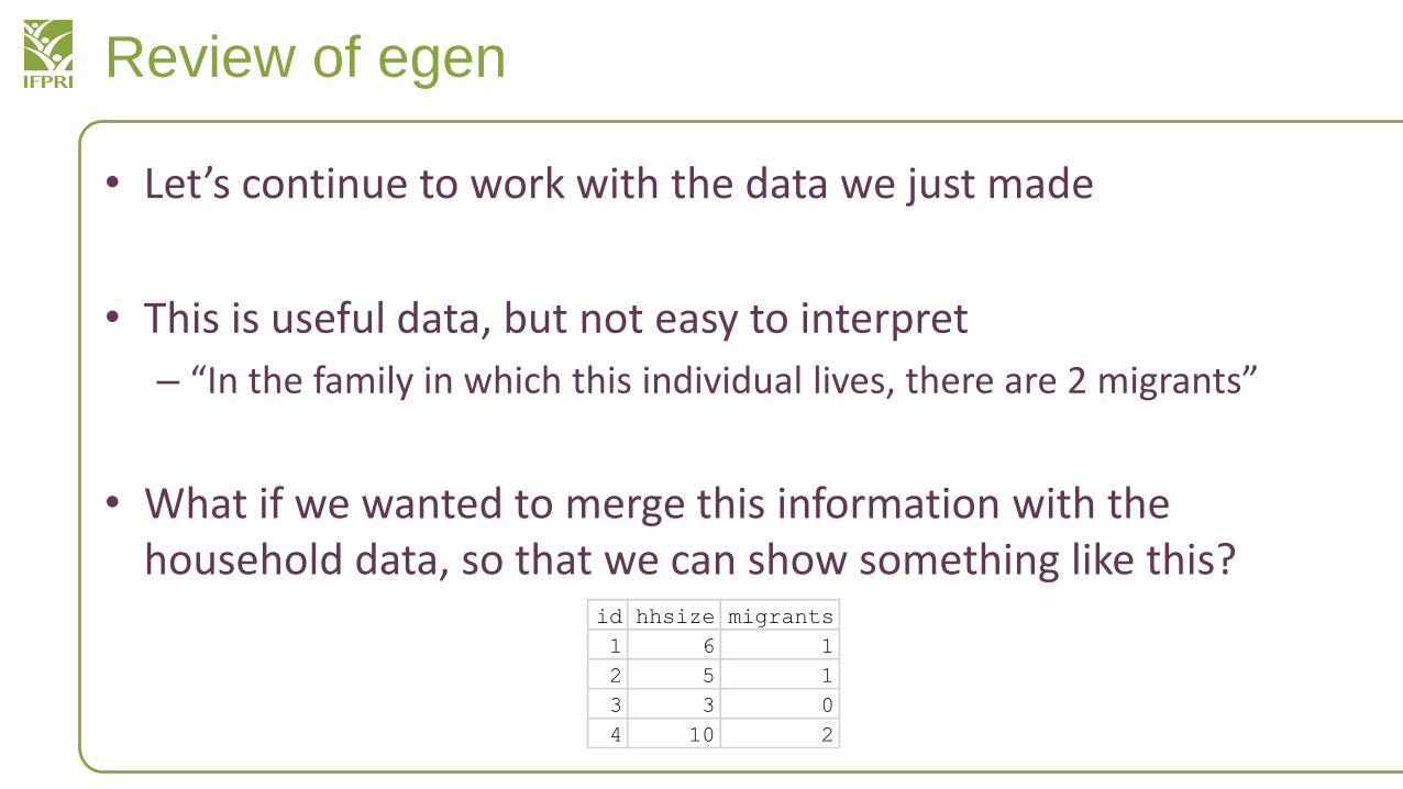
• Let’s continue to work with the data we just made

• This is useful data, but not easy to interpret

– “In the family in which this individual lives, there are 2 migrants”

• What if we wanted to merge this information with the household data, so that we can show something like this?

id hhsize migrants

1 6 1

2 5 1

3 3 0

4 10 2

Advanced Variable Functions: collapse

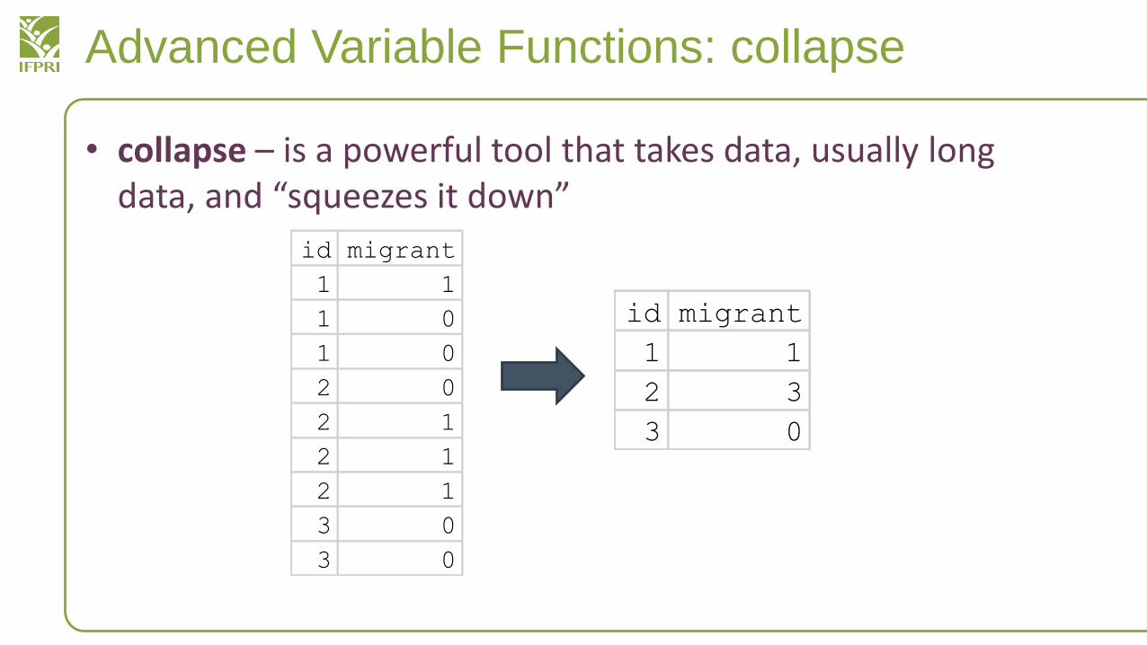
• collapse – is a powerful tool that takes data, usually long data, and “squeezes it down”

id migrant

1 1

1 0

1 0

2 0

2 1

2 1

2 1

3 0

3 0

id migrant

1 1

2 3

3 0

Advanced Variable Functions: collapse

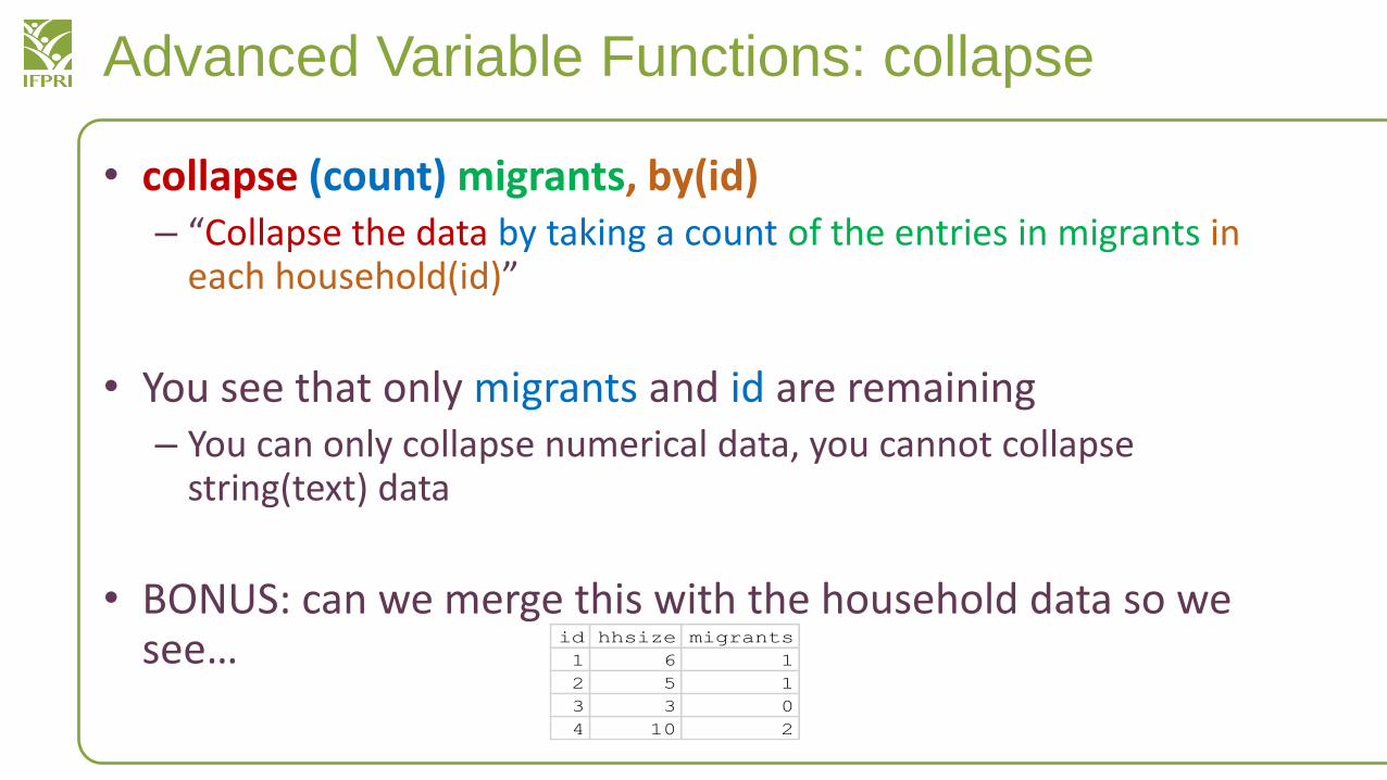
• collapse (count) migrants, by(id)– “Collapse the data by taking a count of the entries in migrants in

each household(id)”

• You see that only migrants and id are remaining– You can only collapse numerical data, you cannot collapse

string(text) data

• BONUS: can we merge this with the household data so we see… id hhsize migrants

1 6 1

2 5 1

3 3 0

4 10 2

Advanced Variable Functions

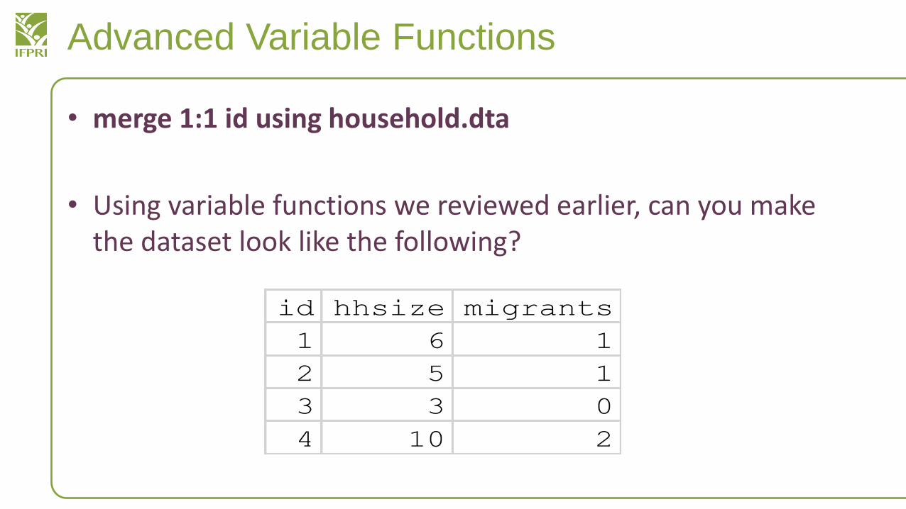
• merge 1:1 id using household.dta

• Using variable functions we reviewed earlier, can you make the dataset look like the following?

id hhsize migrants

1 6 1

2 5 1

3 3 0

4 10 2

Review: Collapse

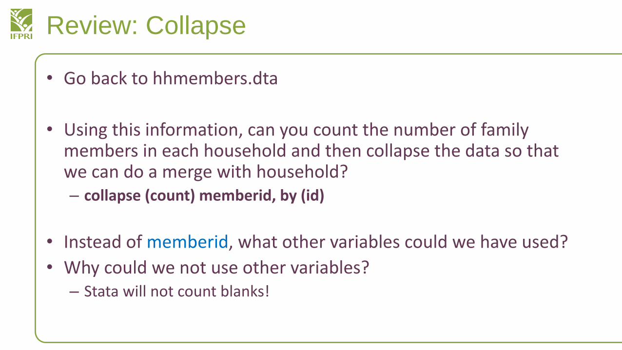
• Go back to hhmembers.dta

• Using this information, can you count the number of family members in each household and then collapse the data so that we can do a merge with household?– collapse (count) memberid, by (id)

• Instead of memberid, what other variables could we have used?

• Why could we not use other variables?– Stata will not count blanks!

Review: Collapse

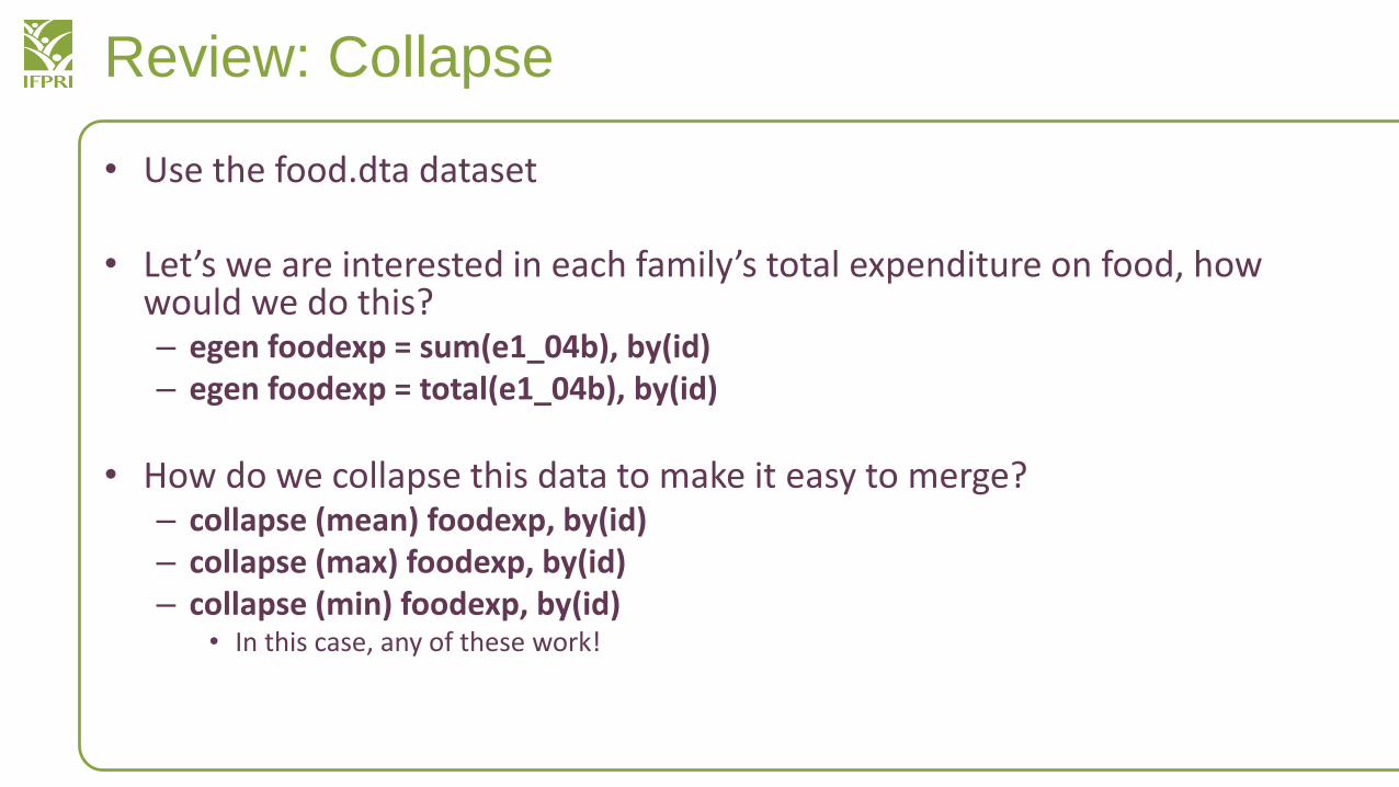
• Use the food.dta dataset

• Let’s we are interested in each family’s total expenditure on food, how would we do this?– egen foodexp = sum(e1_04b), by(id)– egen foodexp = total(e1_04b), by(id)

• How do we collapse this data to make it easy to merge?– collapse (mean) foodexp, by(id)– collapse (max) foodexp, by(id)– collapse (min) foodexp, by(id)

• In this case, any of these work!

Review: Collapse

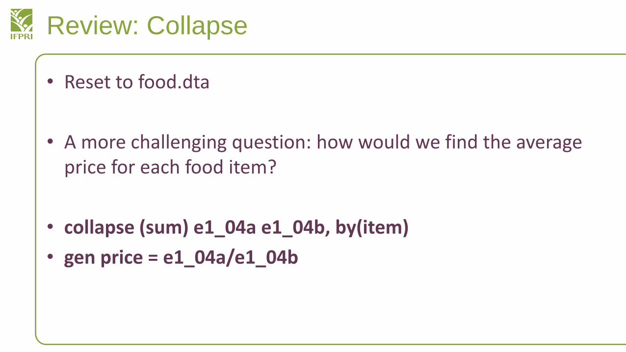
• Reset to food.dta

• A more challenging question: how would we find the average price for each food item?

• collapse (sum) e1_04a e1_04b, by(item)

• gen price = e1_04a/e1_04b

Reshaping Data – Long to Wide

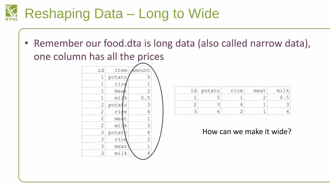
• Remember our food.dta is long data (also called narrow data), one column has all the prices

id item amount

1 potato 5

1 rice 1

1 meat 2

1 milk 0.5

2 potato 3

2 rice 4

2 meat 1

2 milk 3

3 potato 6

3 rice 2

3 meat 1

3 milk 4

id potato rice meat milk

1 5 1 2 0.5

2 3 4 1 3

3 6 2 1 4

How can we make it wide?


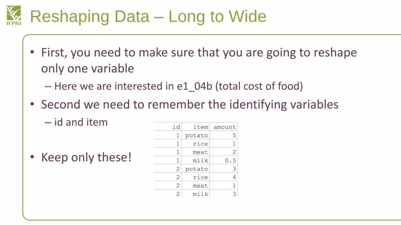
• First, you need to make sure that you are going to reshape only one variable

– Here we are interested in e1_04b (total cost of food)

• Second we need to remember the identifying variables

– id and item

• Keep only these!

id item amount

1 potato 5

1 rice 1

1 meat 2

1 milk 0.5

2 potato 3

2 rice 4

2 meat 1

2 milk 3

3 potato 6

3 rice 2

3 meat 1

3 milk 4


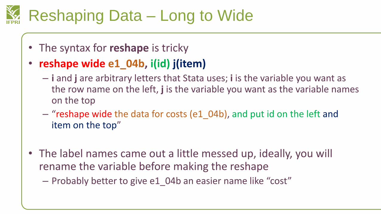
• The syntax for reshape is tricky

• reshape wide e1_04b, i(id) j(item)– i and j are arbitrary letters that Stata uses; i is the variable you want as

the row name on the left, j is the variable you want as the variable names on the top

– “reshape wide the data for costs (e1_04b), and put id on the left and item on the top”

• The label names came out a little messed up, ideally, you will rename the variable before making the reshape– Probably better to give e1_04b an easier name like “cost”

Egen rowtotal

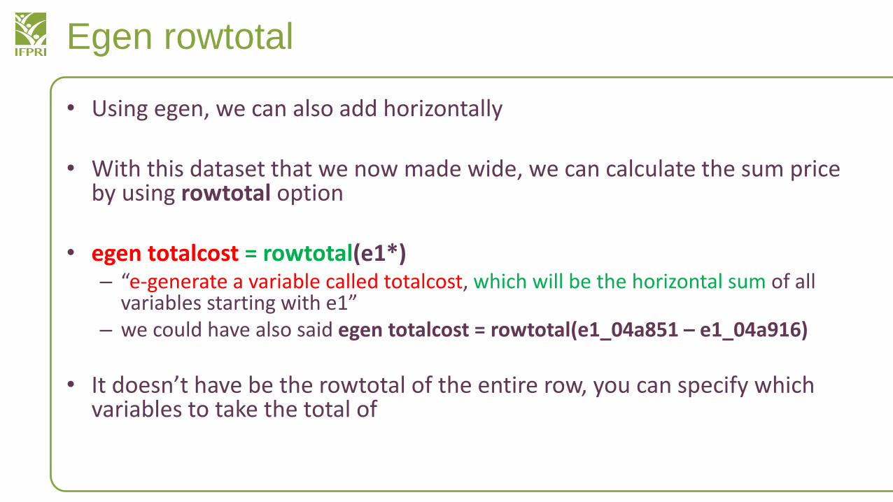
• Using egen, we can also add horizontally

• With this dataset that we now made wide, we can calculate the sum price by using rowtotal option

• egen totalcost = rowtotal(e1*)– “e-generate a variable called totalcost, which will be the horizontal sum of all

variables starting with e1”– we could have also said egen totalcost = rowtotal(e1_04a851 – e1_04a916)

• It doesn’t have be the rowtotal of the entire row, you can specify which variables to take the total of

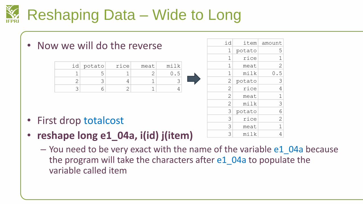
Reshaping Data – Wide to Long

• Now we will do the reverse

• First drop totalcost

• reshape long e1_04a, i(id) j(item)– You need to be very exact with the name of the variable e1_04a because

the program will take the characters after e1_04a to populate the variable called item

id potato rice meat milk

1 5 1 2 0.5

2 3 4 1 3

3 6 2 1 4

id item amount

1 potato 5

1 rice 1

1 meat 2

1 milk 0.5

2 potato 3

2 rice 4

2 meat 1

2 milk 3

3 potato 6

3 rice 2

3 meat 1

3 milk 4

Graphing: Histogram

• Open up the auto dataset (sysuse auto, clear)

• To do a histogram, simply use histogram [variable]

– Let’s say we want a histogram of gas miles per gallon (mpg), how would we do it?

• histogram mpg

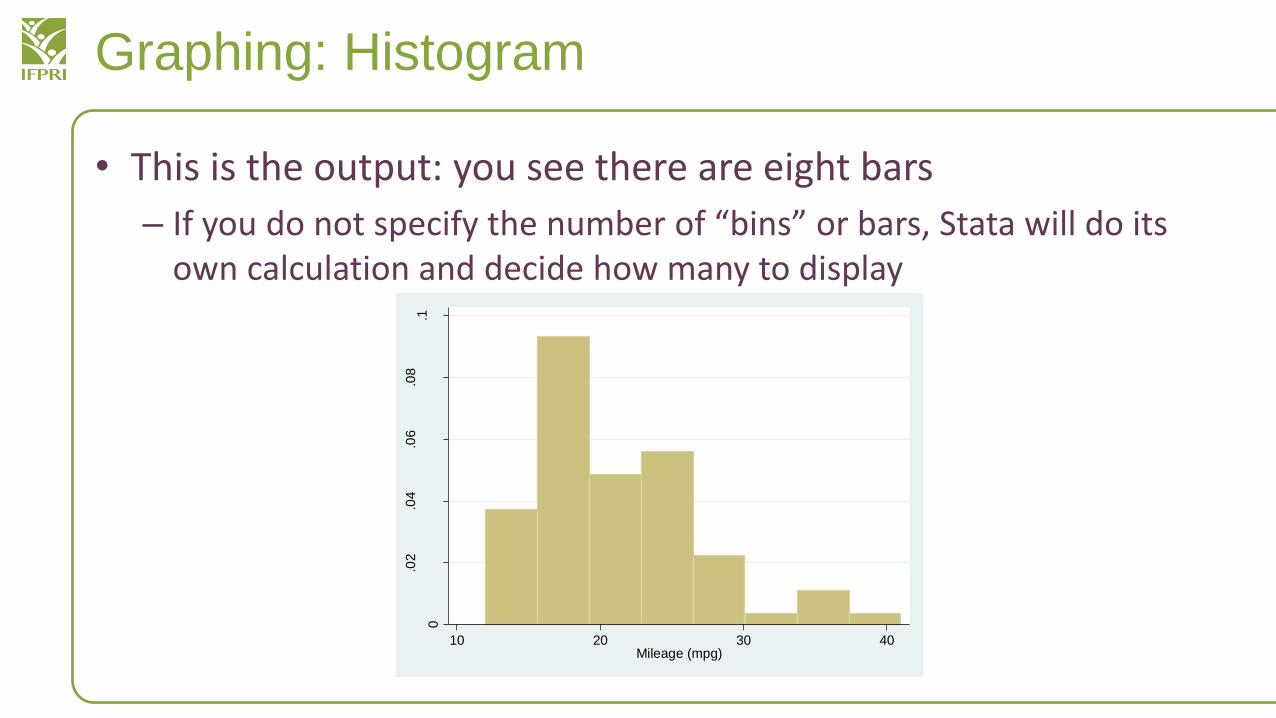
Graphing: Histogram

• This is the output: you see there are eight bars

– If you do not specify the number of “bins” or bars, Stata will do its own calculation and decide how many to display

0

.02

.04

.06

.08

.1

De

nsity

10 20 30 40Mileage (mpg)

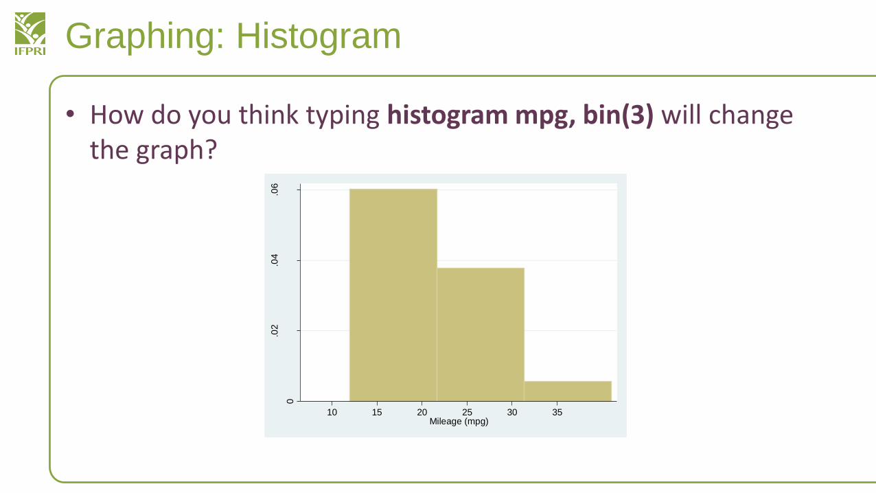
Graphing: Histogram

• How do you think typing histogram mpg, bin(3) will change the graph?

0

.02

.04

.06

De

nsity

10 15 20 25 30 35Mileage (mpg)

Review: Histogram

• Can you make a histogram of household size in our household data?

• Change the number of bars

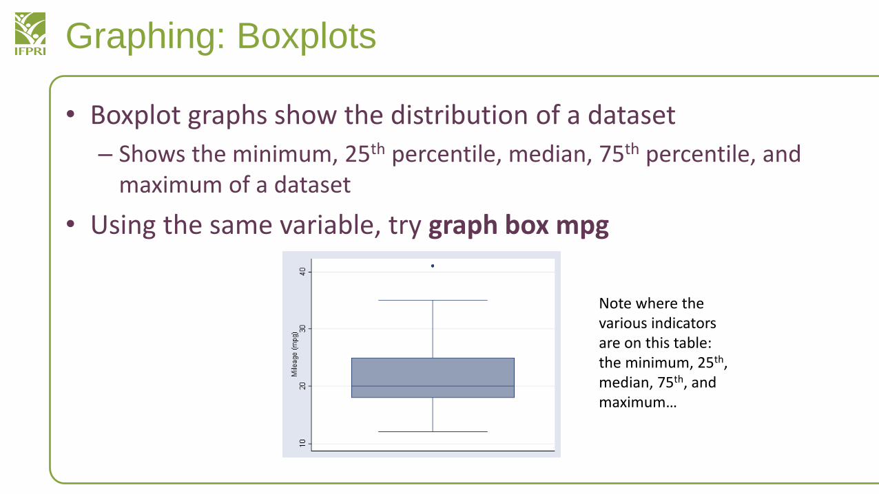
Graphing: Boxplots

• Boxplot graphs show the distribution of a dataset

– Shows the minimum, 25th percentile, median, 75th percentile, and maximum of a dataset

• Using the same variable, try graph box mpg

Note where the various indicators are on this table: the minimum, 25th, median, 75th, and maximum…

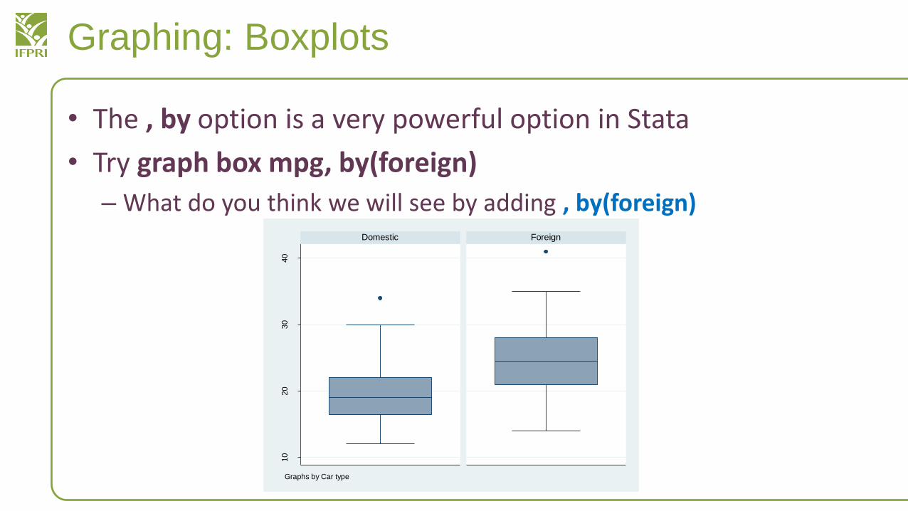
Graphing: Boxplots

• The , by option is a very powerful option in Stata

• Try graph box mpg, by(foreign)

– What do you think we will see by adding , by(foreign)

10

20

30

40

Domestic Foreign

Mile

age

(m

pg)

Graphs by Car type

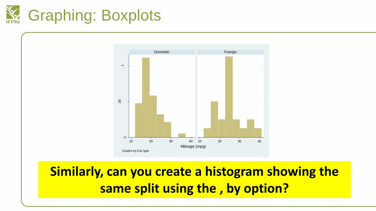
Graphing: Boxplots

0

.05

.1

10 20 30 40 10 20 30 40

Domestic Foreign

De

nsity

Mileage (mpg)Graphs by Car type

Similarly, can you create a histogram showing the same split using the , by option?

Graphing: Pie Charts

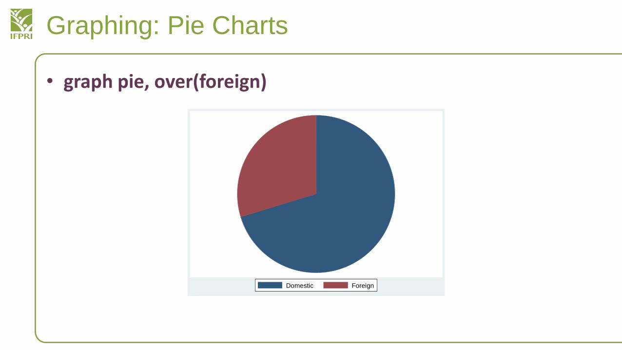
• graph pie, over(foreign)

Domestic Foreign

Graphing: Pie Charts

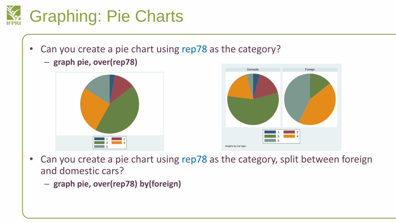
• Can you create a pie chart using rep78 as the category?– graph pie, over(rep78)

• Can you create a pie chart using rep78 as the category, split between foreign and domestic cars?– graph pie, over(rep78) by(foreign)

1 2

3 4

5

Domestic Foreign

1 2

3 4

5

Graphs by Car type

Graphing: Two-Way

• Two way plots can either be a scatter or line plot

– You can create them with graph twoway scatter or graph twowayline

• graph twoway scatter mpg weight – to see a scatter plot of gas miles per gallon vs. car weight

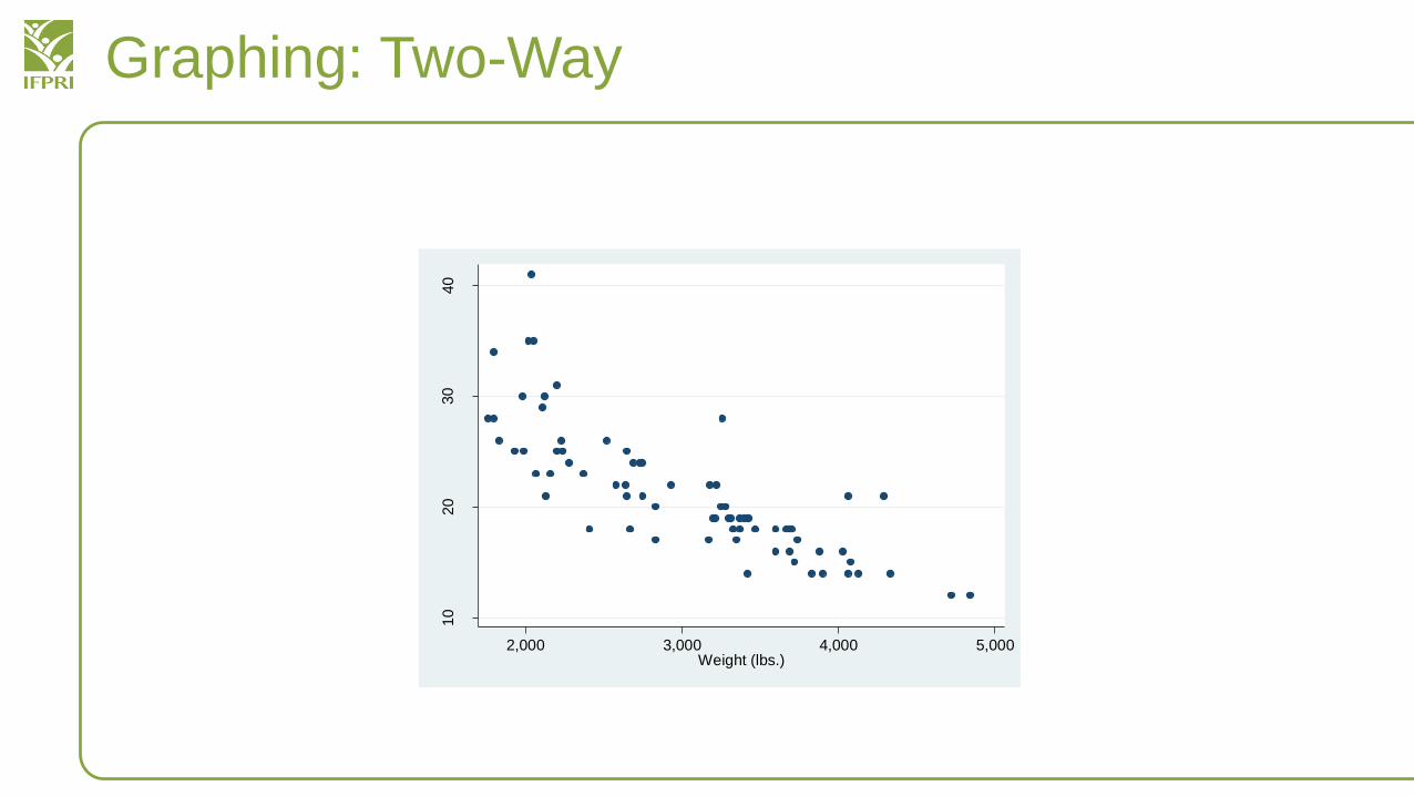
Graphing: Two-Way

10

20

30

40

Mile

age

(m

pg)

2,000 3,000 4,000 5,000Weight (lbs.)

Graphing: Two Way

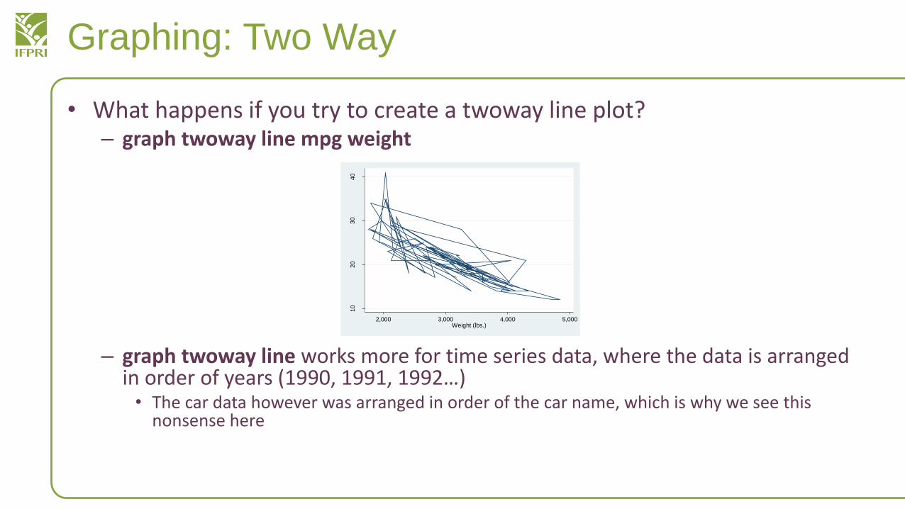
• What happens if you try to create a twoway line plot?– graph twoway line mpg weight

– graph twoway line works more for time series data, where the data is arranged in order of years (1990, 1991, 1992…)

• The car data however was arranged in order of the car name, which is why we see this nonsense here

10

20

30

40

Mile

age

(m

pg)

2,000 3,000 4,000 5,000Weight (lbs.)

Graphing: Two Way

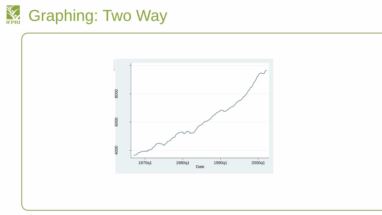
• Here is a better example where you can use graph twowayline

• From our earlier dataset on GNP over time:

– sysuse gnp96, clear

– graph twoway line gnp96 date

Graphing: Two Way

40

00

60

00

80

00

10

00

0

Re

al G

ross N

ationa

l P

rod

uct

1970q1 1980q1 1990q1 2000q1Date

Day 5: Preview

• Finishing graphs

• T-Test

• Regression and Analysis

Graphing: Two Way

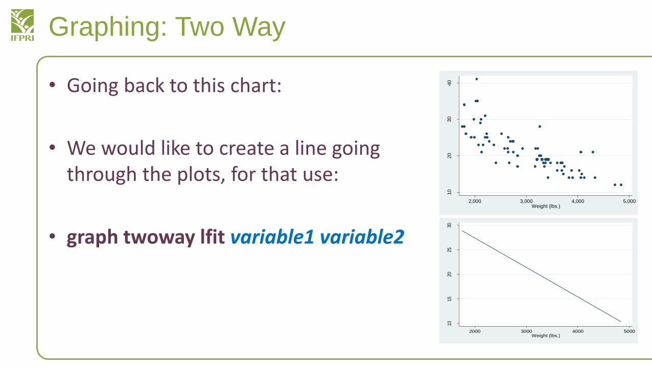
• Going back to this chart:

• We would like to create a line going through the plots, for that use:

• graph twoway lfit variable1 variable2

10

20

30

40

Mile

age

(m

pg)

2,000 3,000 4,000 5,000Weight (lbs.)

10

15

20

25

30

Fitt

ed

va

lues

2000 3000 4000 5000Weight (lbs.)

Graphing: Two Way

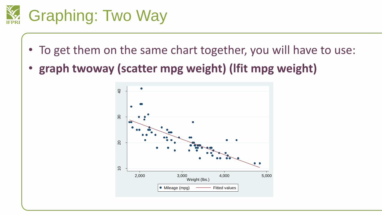
• To get them on the same chart together, you will have to use:

• graph twoway (scatter mpg weight) (lfit mpg weight)

10

20

30

40

2,000 3,000 4,000 5,000Weight (lbs.)

Mileage (mpg) Fitted values

Graphing: Two Way

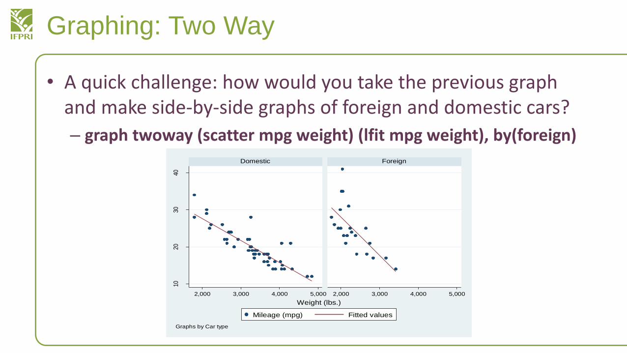
• A quick challenge: how would you take the previous graph and make side-by-side graphs of foreign and domestic cars?

– graph twoway (scatter mpg weight) (lfit mpg weight), by(foreign)

1020

3040

2,000 3,000 4,000 5,000 2,000 3,000 4,000 5,000

Domestic Foreign

Mileage (mpg) Fitted values

Weight (lbs.)

Graphs by Car type

T-test: One Sample

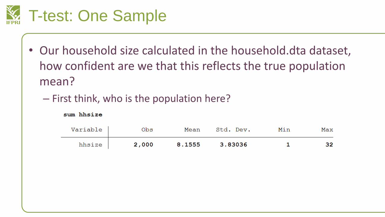
• Our household size calculated in the household.dta dataset, how confident are we that this reflects the true population mean?

– First think, who is the population here?

T-Test: One Sample

• Let’s set up our null and alternative hypothesis:– Null hypothesis (H0) = Population mean is 7.5– Alt. hypothesis (HA) = Population mean is not 7.5

• 7.5 here is an arbitrary figure, you can do this for any other number

• Before making any statements, we need to make a few assumptions:– Normal distribution – most values are concentrated around the mean:

more like to have family size of 7 or 9 than 2 or 15– Independent measurement – every family had equal chance of being

surveyed; enumerator didn’t look at large families and said “I don’t want interview them”

T-test: One Sample

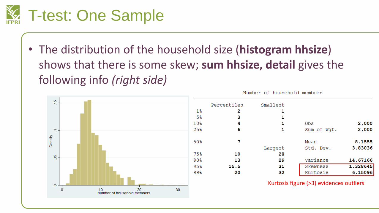
• The distribution of the household size (histogram hhsize)shows that there is some skew; sum hhsize, detail gives the following info (right side)

Kurtosis figure (>3) evidences outliers

T-Test: One Sample

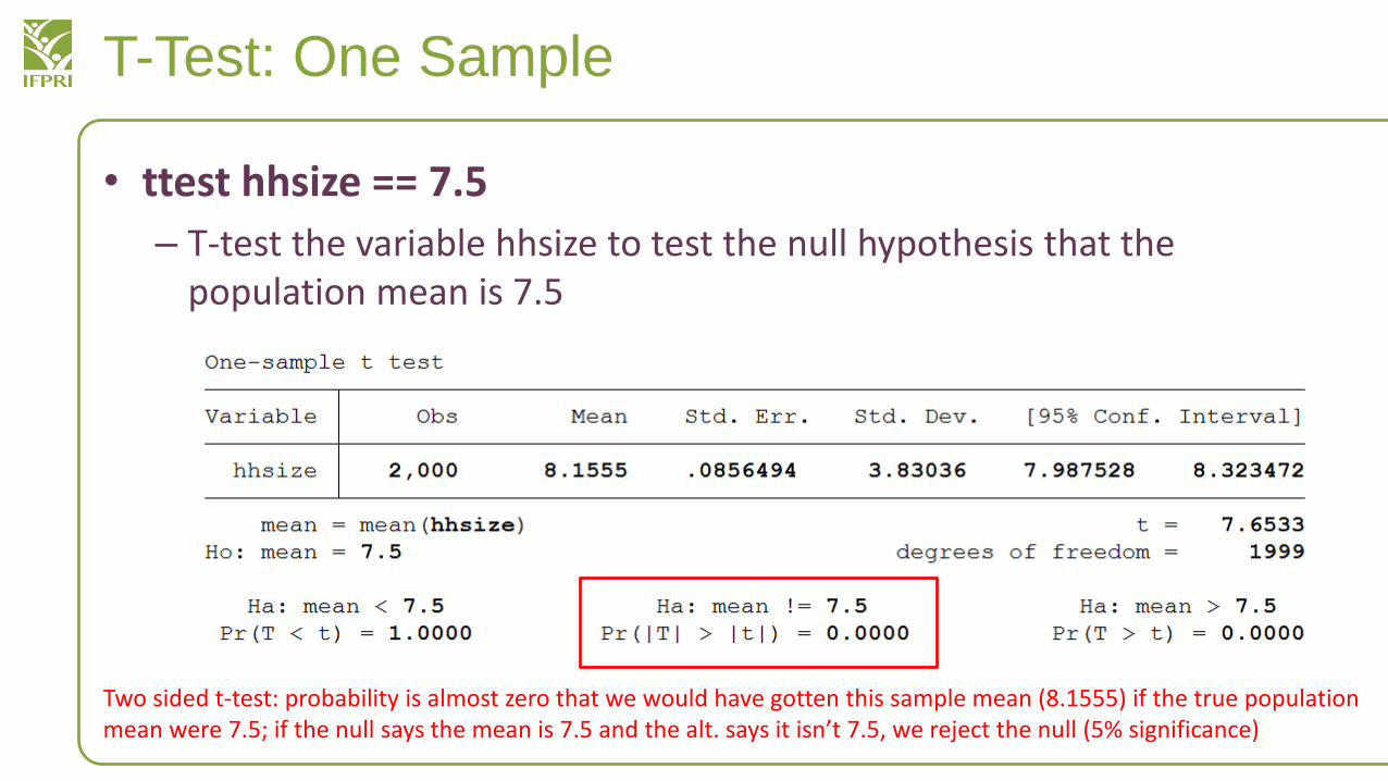
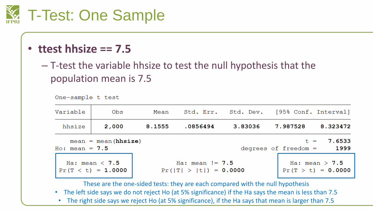
• ttest hhsize == 7.5

– T-test the variable hhsize to test the null hypothesis that the population mean is 7.5

Two sided t-test: probability is almost zero that we would have gotten this sample mean (8.1555) if the true population mean were 7.5; if the null says the mean is 7.5 and the alt. says it isn’t 7.5, we reject the null (5% significance)

T-Test: One Sample

• Given our null hypothesis: that the population mean is 7.5• And our alternative hypothesis: that the pop mean isn’t 7.5

• Given these two options, we can reject the null hypothesis

• The probability is almost zero that the null hypothesis is true and we got these results

• At 95% percent confidence, 5% significance, we reject all null hypothesis that is under p-value 0.05

T-Test: One Sample

• ttest hhsize == 7.5

– T-test the variable hhsize to test the null hypothesis that the population mean is 7.5

These are the one-sided tests: they are each compared with the null hypothesis• The left side says we do not reject Ho (at 5% significance) if the Ha says the mean is less than 7.5• The right side says we reject Ho (at 5% significance), if the Ha says that mean is larger than 7.5

T-Test: One Sample

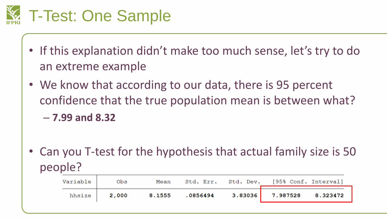
• If this explanation didn’t make too much sense, let’s try to do an extreme example

• We know that according to our data, there is 95 percent confidence that the true population mean is between what?

– 7.99 and 8.32

• Can you T-test for the hypothesis that actual family size is 50 people?

T-Test: One Sample

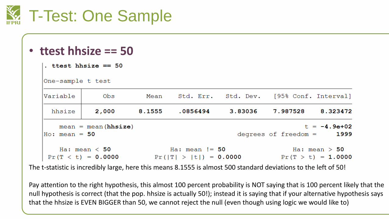
• ttest hhsize == 50

The t-statistic is incredibly large, here this means 8.1555 is almost 500 standard deviations to the left of 50!

Pay attention to the right hypothesis, this almost 100 percent probability is NOT saying that is 100 percent likely that the null hypothesis is correct (that the pop. hhsize is actually 50!); instead it is saying that if your alternative hypothesis says that the hhsize is EVEN BIGGER than 50, we cannot reject the null (even though using logic we would like to)

T-Test: Two Samples

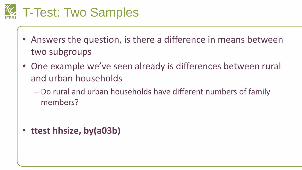
• Answers the question, is there a difference in means between two subgroups

• One example we’ve seen already is differences between rural and urban households

– Do rural and urban households have different numbers of family members?

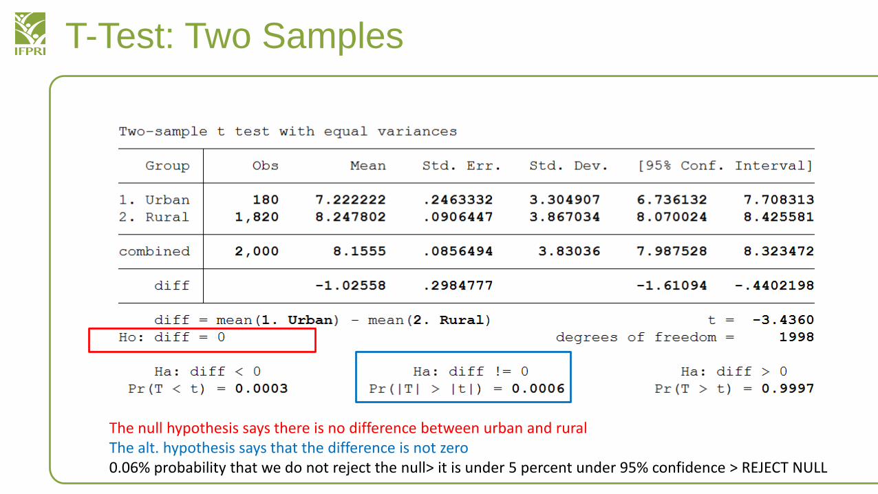
• ttest hhsize, by(a03b)

T-Test: Two Samples

The null hypothesis says there is no difference between urban and ruralThe alt. hypothesis says that the difference is not zero0.06% probability that we do not reject the null> it is under 5 percent under 95% confidence > REJECT NULL

T-Test: Two Samples

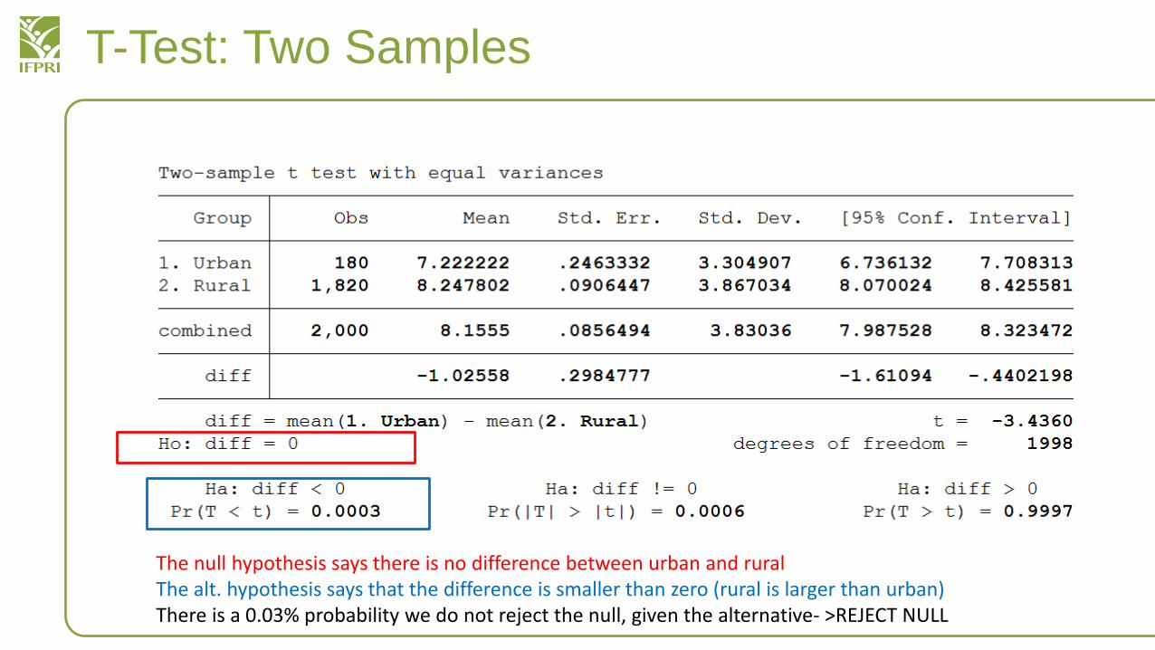
The null hypothesis says there is no difference between urban and ruralThe alt. hypothesis says that the difference is smaller than zero (rural is larger than urban)There is a 0.03% probability we do not reject the null, given the alternative- >REJECT NULL

T-Test: Two Samples

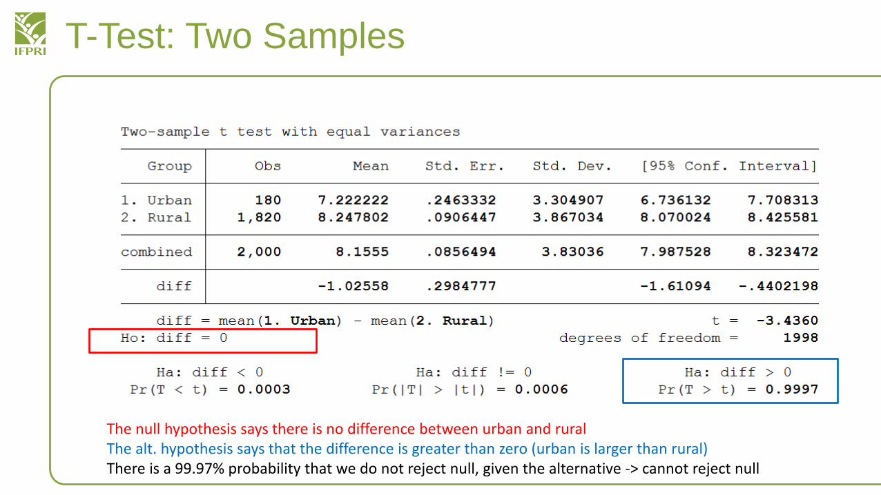
The null hypothesis says there is no difference between urban and ruralThe alt. hypothesis says that the difference is greater than zero (urban is larger than rural)There is a 99.97% probability that we do not reject null, given the alternative -> cannot reject null

Linear Regression and Data Analysis

• Because our own dataset may not be particularly illustrative of regression analysis, let’s use sysuse lifeexp and merge in the doctor.dta using the country variable– merge 1:1 country using doctor

• What aspects are related to life expectancy?• First, describe the dataset so we know what we are working with• label var safewater “Percent access to safe drinking water”• label var doctor “Doctors per 1,000 population”

• Before we regress this data, let’s quickly look at the descriptive statistics, although we probably have good hypotheses already


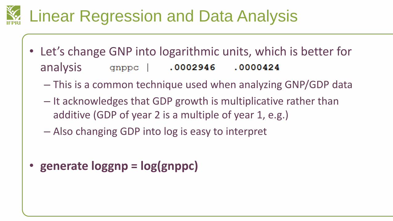
• Let’s change GNP into logarithmic units, which is better for analysis

– This is a common technique used when analyzing GNP/GDP data

– It acknowledges that GDP growth is multiplicative rather than additive (GDP of year 2 is a multiple of year 1, e.g.)

– Also changing GDP into log is easy to interpret

• generate loggnp = log(gnppc)


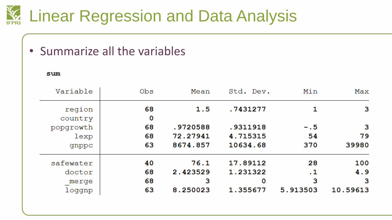
• Summarize all the variables


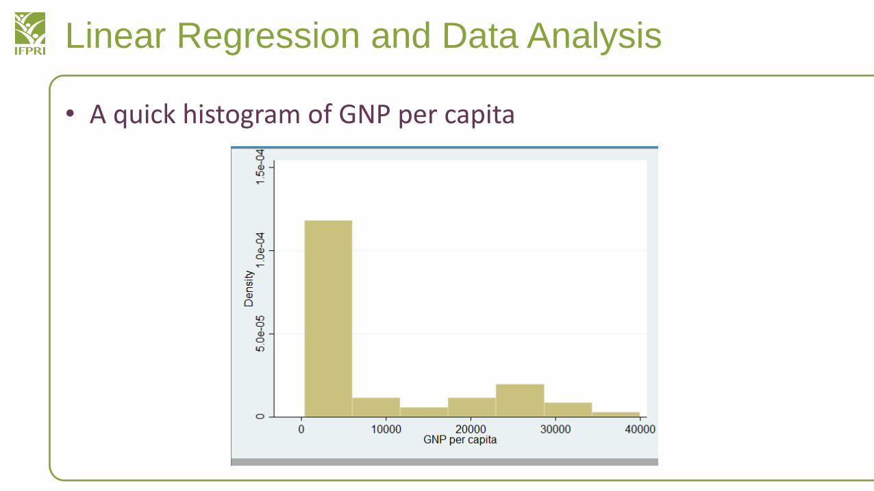
• A quick histogram of GNP per capita


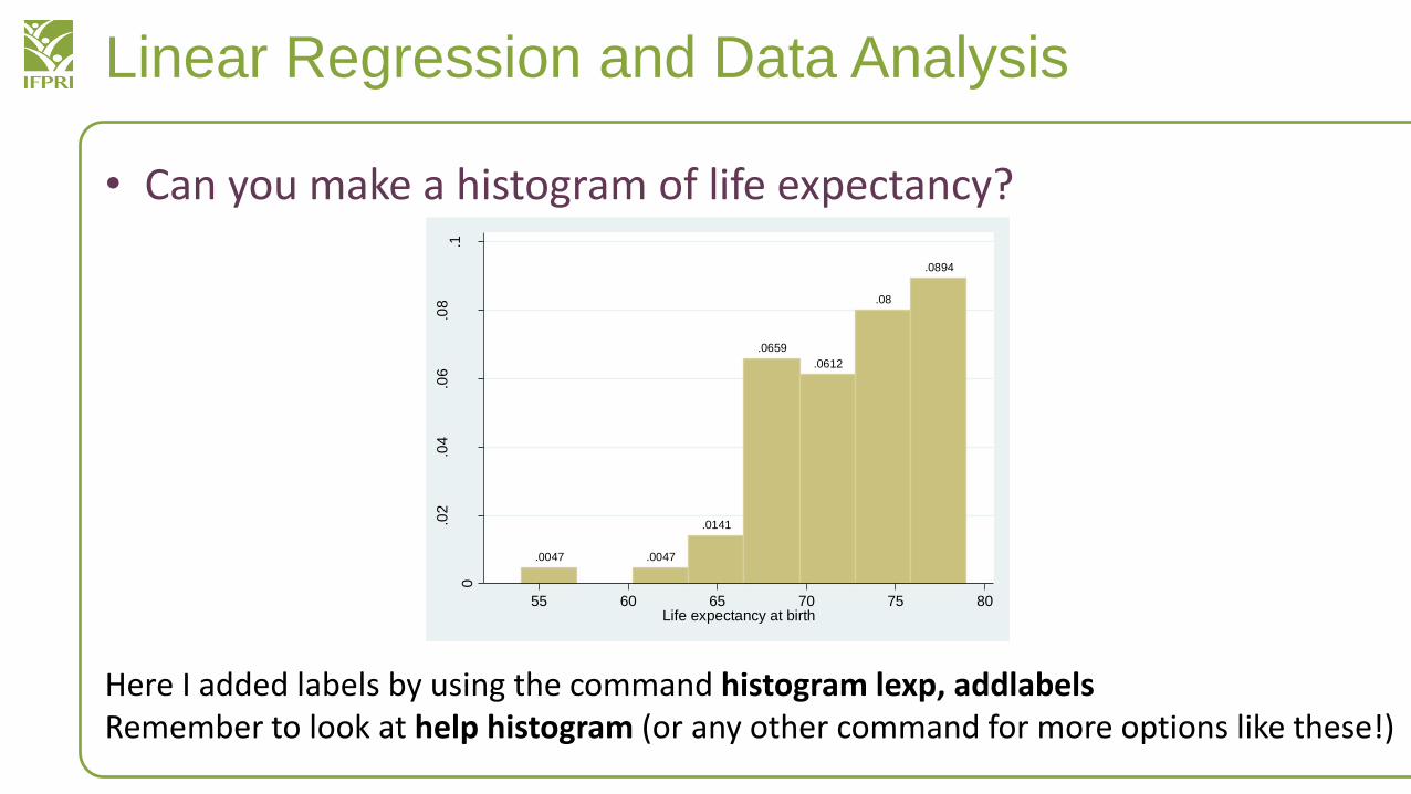
• Can you make a histogram of life expectancy?

.0047 .0047

.0141

.0659

.0612

.08

.0894

0

.02

.04

.06

.08

.1

De

nsity

55 60 65 70 75 80Life expectancy at birth

Here I added labels by using the command histogram lexp, addlabelsRemember to look at help histogram (or any other command for more options like these!)


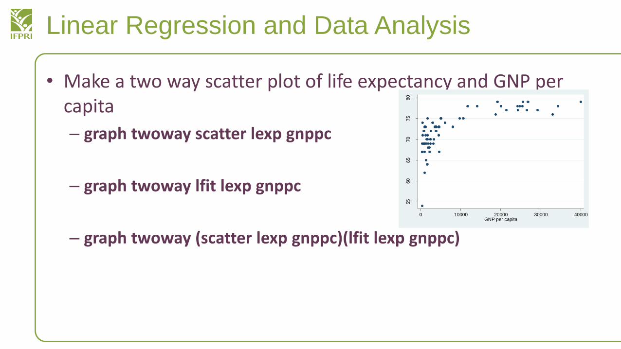
• Make a two way scatter plot of life expectancy and GNP per capita

– graph twoway scatter lexp gnppc

– graph twoway lfit lexp gnppc

– graph twoway (scatter lexp gnppc)(lfit lexp gnppc)

55

60

65

70

75

80

Life

expe

cta

ncy a

t bir

th

0 10000 20000 30000 40000GNP per capita


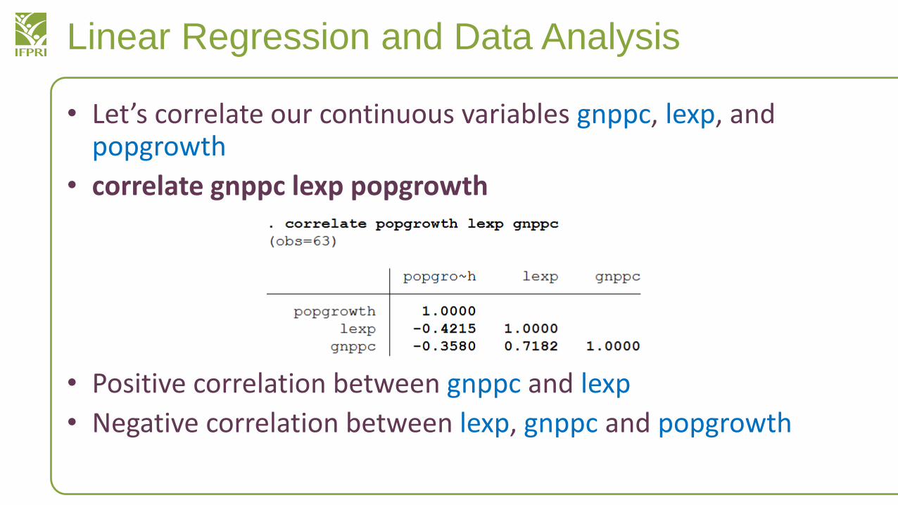
• Let’s correlate our continuous variables gnppc, lexp, and popgrowth

• correlate gnppc lexp popgrowth

• Positive correlation between gnppc and lexp

• Negative correlation between lexp, gnppc and popgrowth


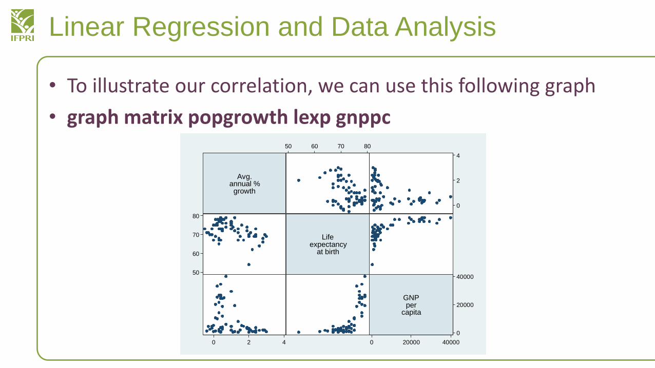
• To illustrate our correlation, we can use this following graph

• graph matrix popgrowth lexp gnppc

Avg.annual %growth

Lifeexpectancy

at birth

GNPper

capita

0

2

4

0 2 4

50

60

70

80

50 60 70 80

0

20000

40000

0 20000 40000


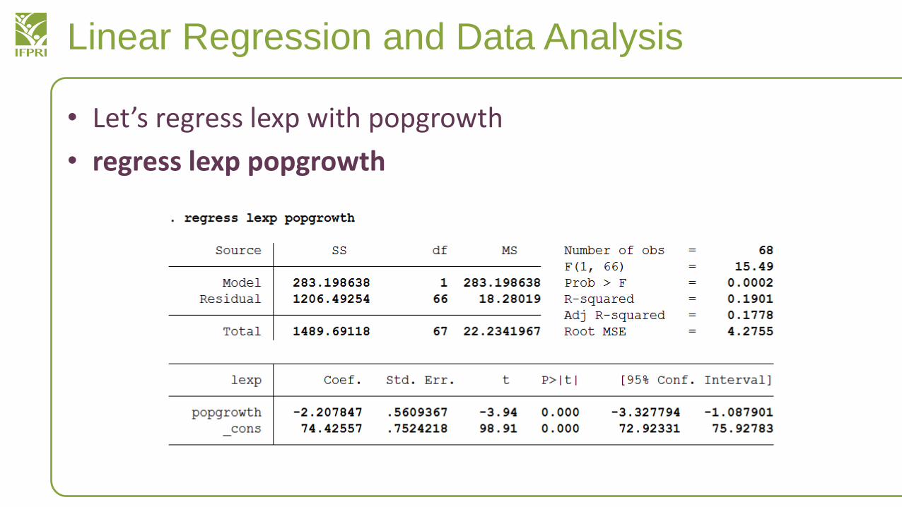
• Let’s regress lexp with popgrowth

• regress lexp popgrowth


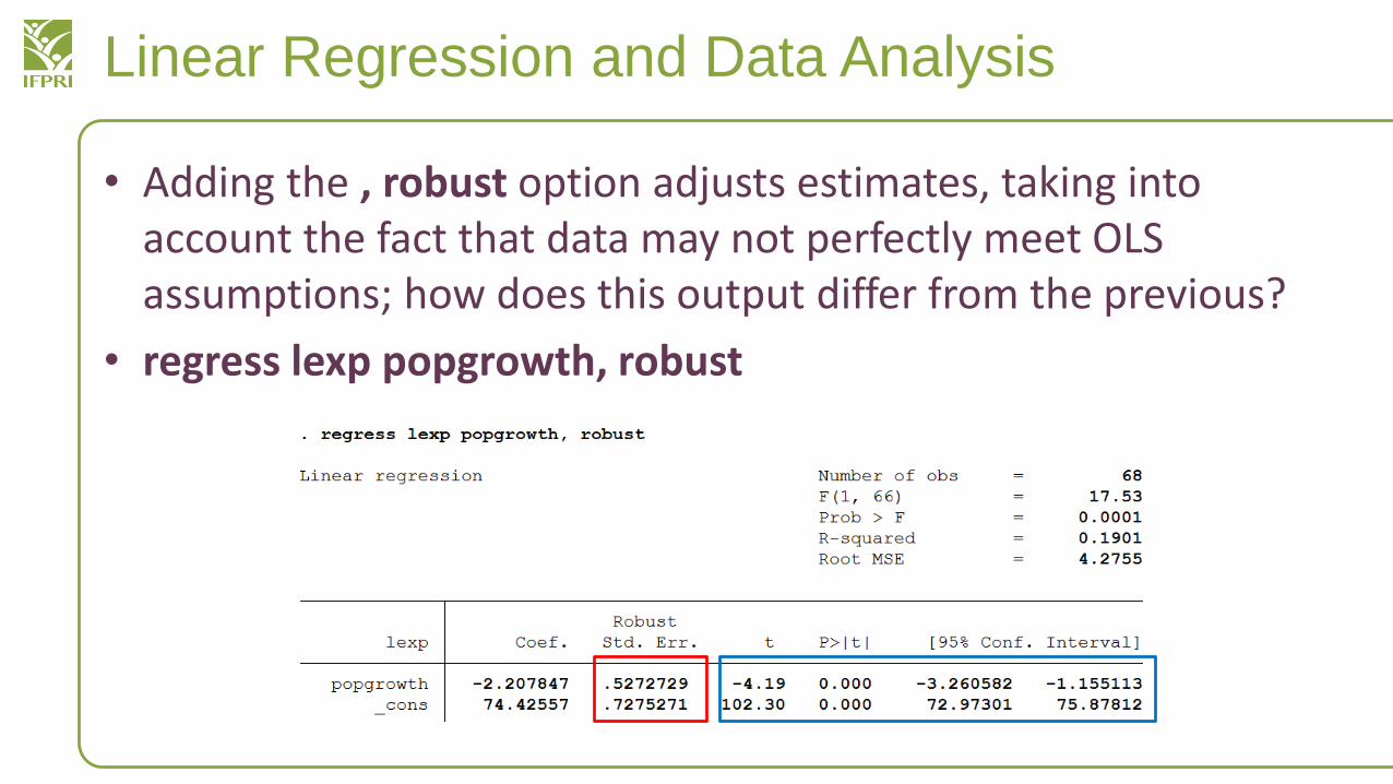
• Adding the , robust option adjusts estimates, taking into account the fact that data may not perfectly meet OLS assumptions; how does this output differ from the previous?

• regress lexp popgrowth, robust


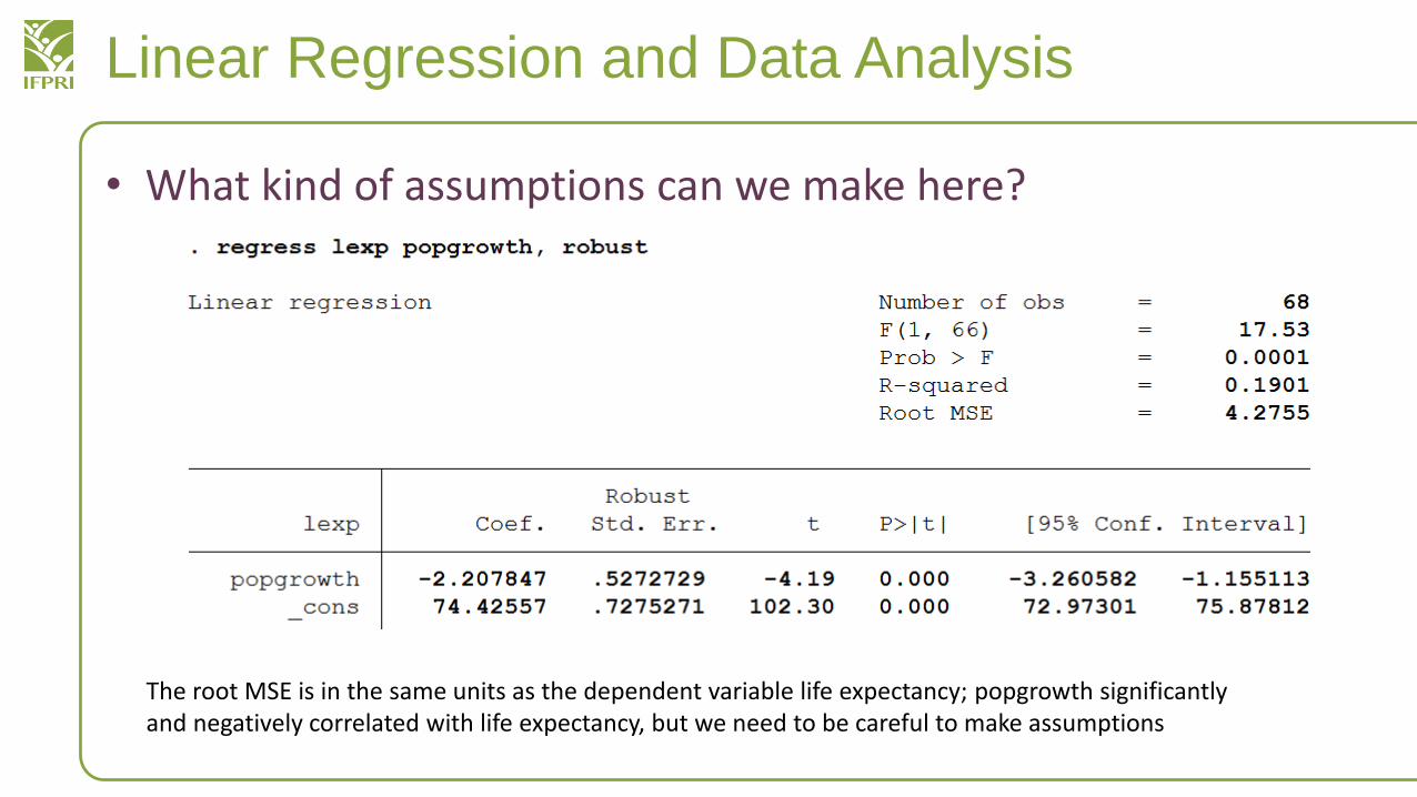
• What kind of assumptions can we make here?

The root MSE is in the same units as the dependent variable life expectancy; popgrowth significantly and negatively correlated with life expectancy, but we need to be careful to make assumptions

Linear Regression

• There were obvious issues with the variable popgrowth

• We need to frame our research question with a better hypothesis

• What effect does GNP per capita have on life expectancy?

Linear Regression

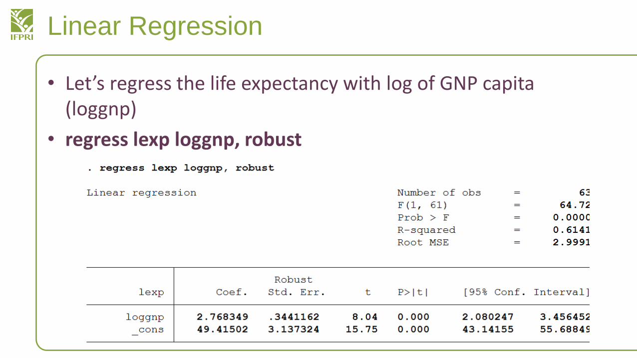
• Let’s regress the life expectancy with log of GNP capita (loggnp)

• regress lexp loggnp, robust

Linear Regression: Verifying OLS Assumptions

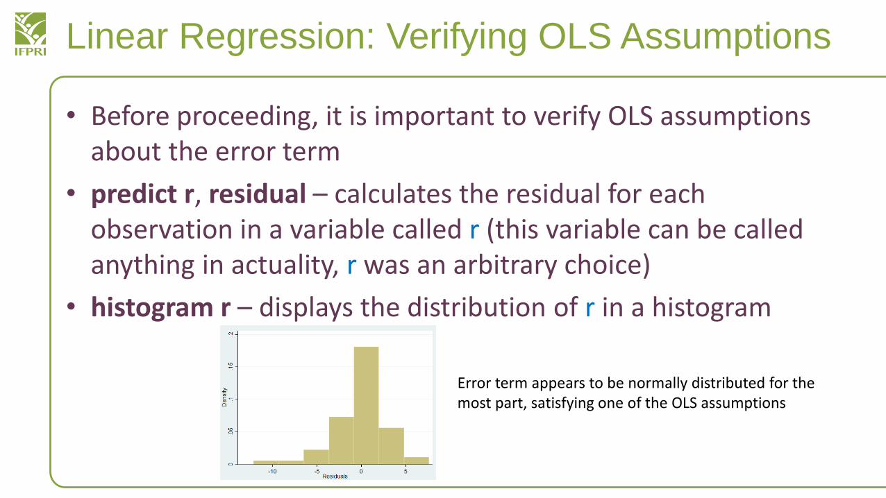
• Before proceeding, it is important to verify OLS assumptions about the error term

• predict r, residual – calculates the residual for each observation in a variable called r (this variable can be called anything in actuality, r was an arbitrary choice)

• histogram r – displays the distribution of r in a histogram

Error term appears to be normally distributed for the most part, satisfying one of the OLS assumptions

Linear Regression: Verifying OLS Assumptions

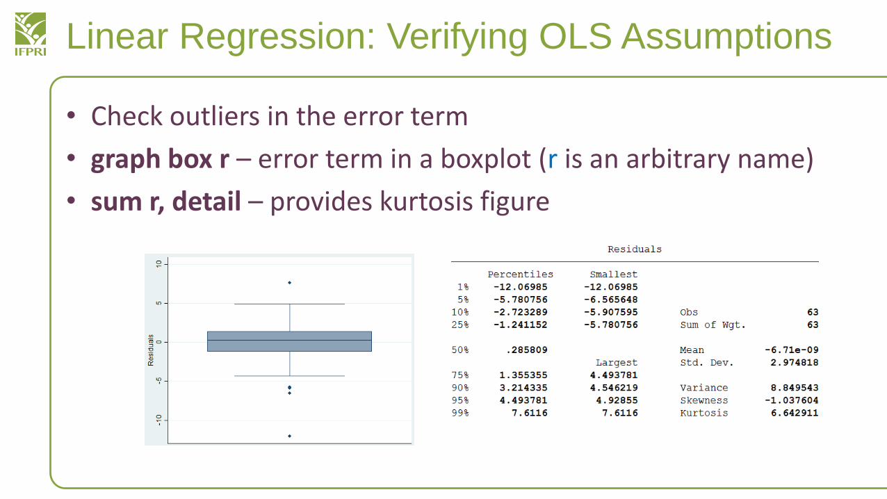
• Check outliers in the error term

• graph box r – error term in a boxplot (r is an arbitrary name)

• sum r, detail – provides kurtosis figure


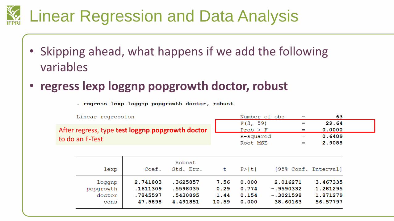
• Skipping ahead, what happens if we add the following variables

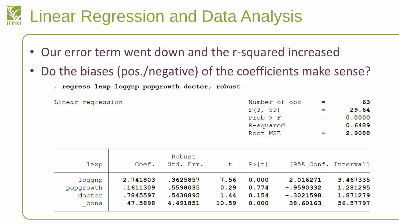
• regress lexp loggnp popgrowth doctor, robust

After regress, type test loggnp popgrowth doctor to do an F-Test


• The previous slide was included to show how to enter multiple independent variables in the regress command

• Bear in mind that you should not “skip steps” in the process

• Selection of variables should be done carefully with the right set of policy questions, assumptions, and considerations of omitted variable bias and multicollinearity in mind


• Our error term went down and the r-squared increased

• Do the biases (pos./negative) of the coefficients make sense?


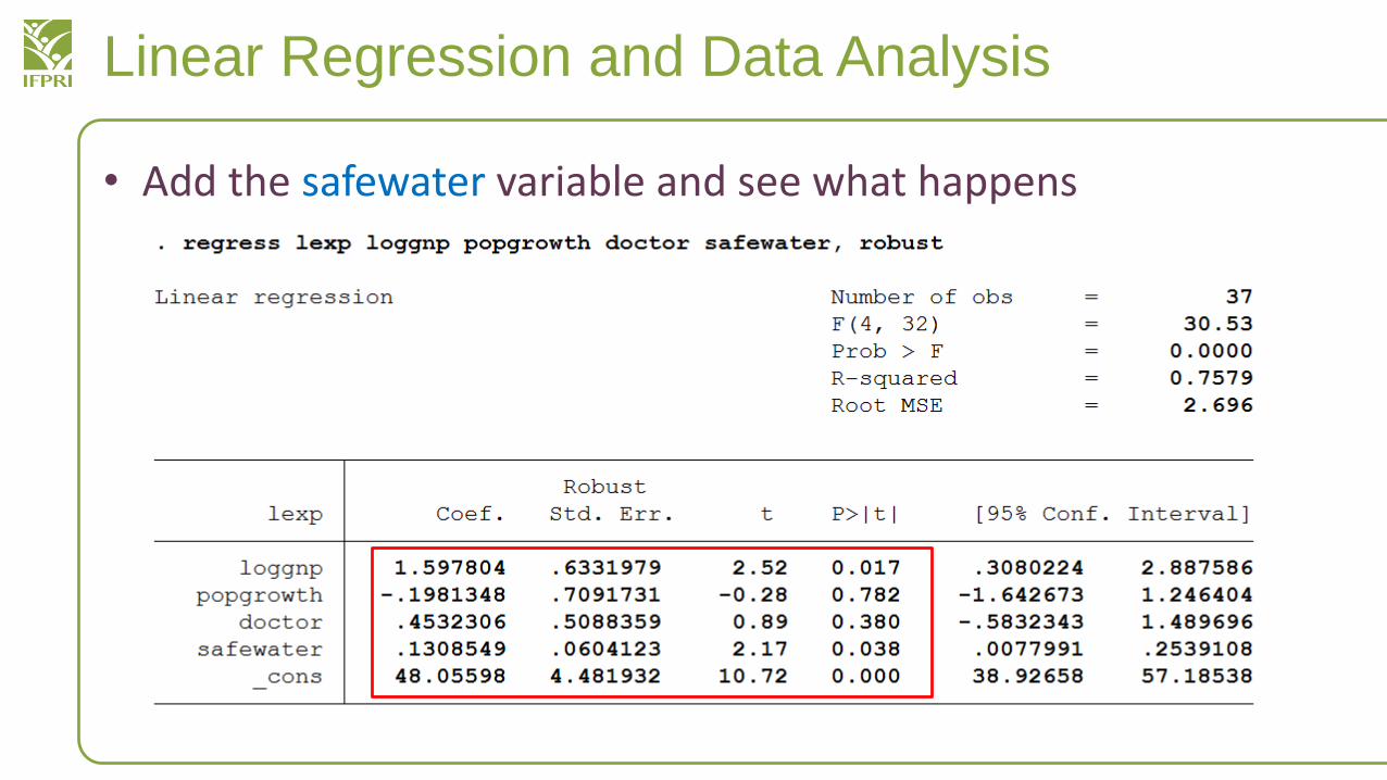
• Add the safewater variable and see what happens


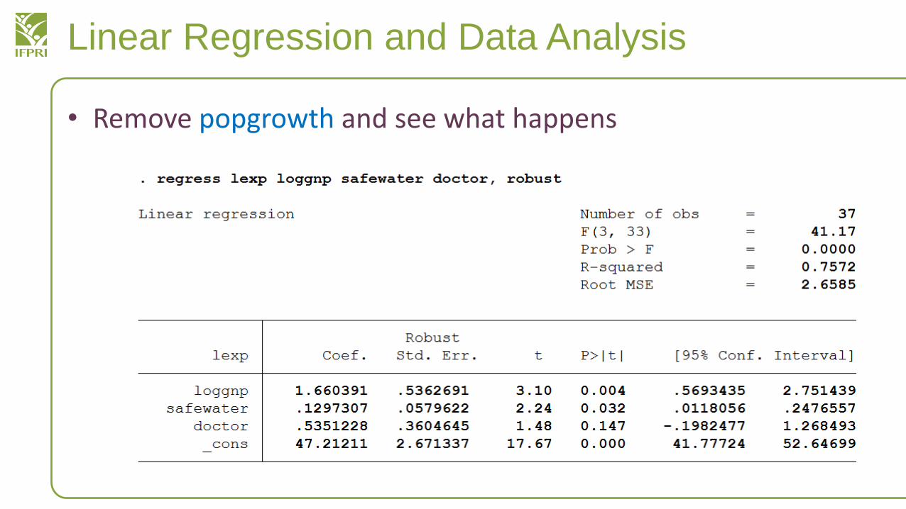
• Remove popgrowth and see what happens


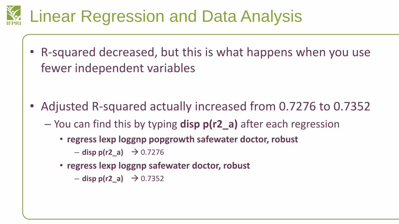
• R-squared decreased, but this is what happens when you use fewer independent variables

• Adjusted R-squared actually increased from 0.7276 to 0.7352

– You can find this by typing disp p(r2_a) after each regression

• regress lexp loggnp popgrowth safewater doctor, robust– disp p(r2_a) 0.7276

• regress lexp loggnp safewater doctor, robust

– disp p(r2_a) 0.7352

Stepwise Command

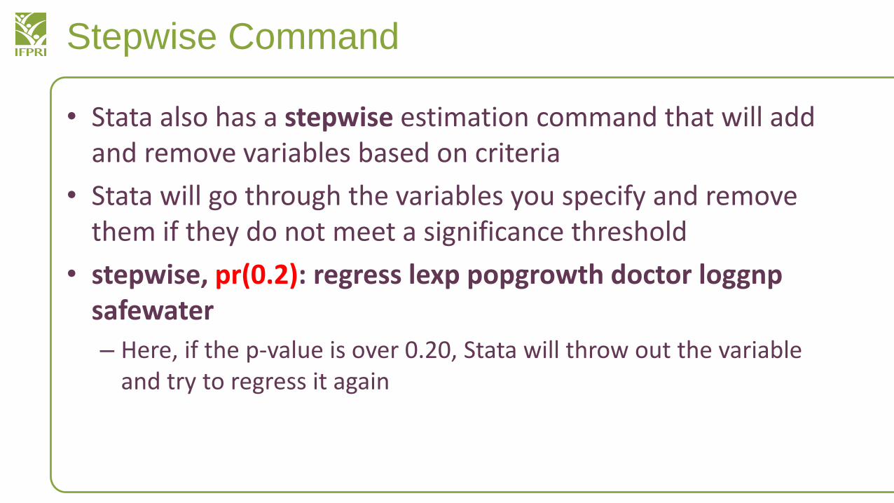
• Stata also has a stepwise estimation command that will add and remove variables based on criteria

• Stata will go through the variables you specify and remove them if they do not meet a significance threshold

• stepwise, pr(0.2): regress lexp popgrowth doctor loggnpsafewater

– Here, if the p-value is over 0.20, Stata will throw out the variable and try to regress it again

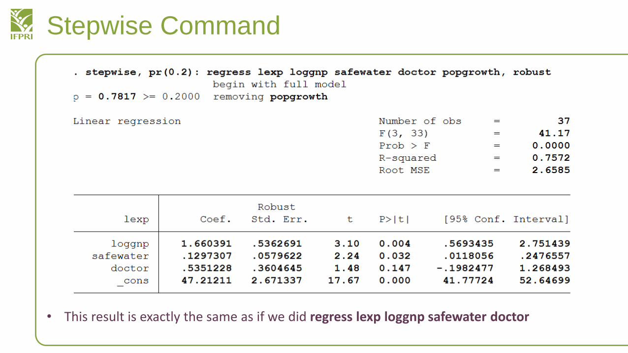
Stepwise Command

• This result is exactly the same as if we did regress lexp loggnp safewater doctor

Stepwise Command

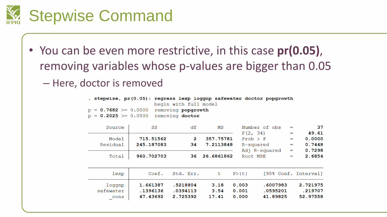
• You can be even more restrictive, in this case pr(0.05), removing variables whose p-values are bigger than 0.05

– Here, doctor is removed

Stepwise Command

• Stepwise estimation can be a useful tool, but needs to be applied with great caution– Statistical significance of results is overestimated because

estimations of previous regressions are ignored

– Result does not document other possible combinations of regressors and their interactions

• Better to base regression on context and theory; stepwise does not take these factors into account

• Focus on theoretical considerations and document all specifications and their interactions

Specification Criteria: Include Variable or Not?

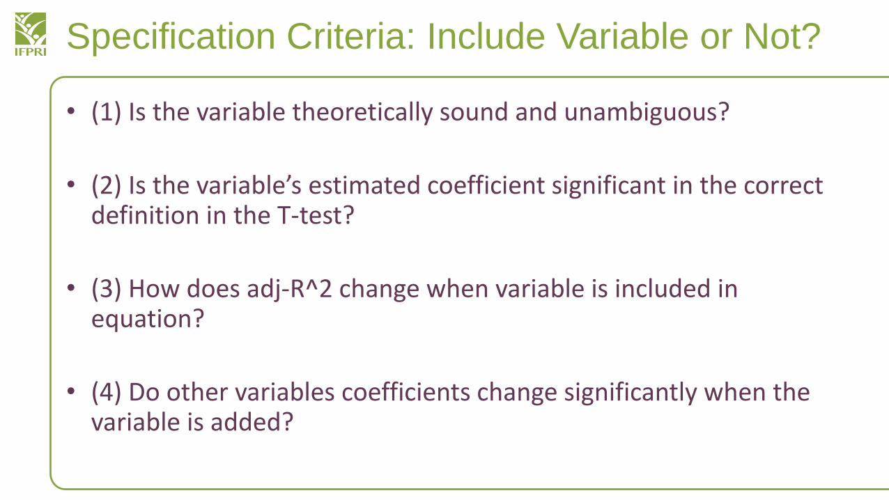
• (1) Is the variable theoretically sound and unambiguous?

• (2) Is the variable’s estimated coefficient significant in the correct definition in the T-test?

• (3) How does adj-R^2 change when variable is included in equation?

• (4) Do other variables coefficients change significantly when the variable is added?

Egen/Collapse/Merge/TTest: Review Exercise #1

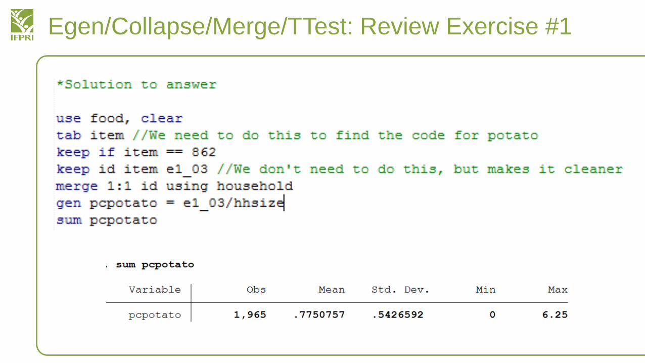
• In small groups, try the following exercise that brings together a lot of our knowledge

• Can you calculate per capita consumption of potatoes in households (amount of potatoes eaten by each person)?– What is the average household amount of potatoes consumed?– Note: This dataset describes a week’s worth of consumption

• After you calculate the per capita consumption of potatoes, compare it to a null hypothesis that actual per capita consumption is 1 kilo per person per week


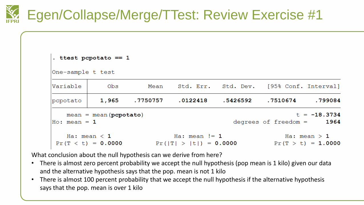
What conclusion about the null hypothesis can we derive from here?• There is almost zero percent probability we accept the null hypothesis (pop mean is 1 kilo) given our data

and the alternative hypothesis says that the pop. mean is not 1 kilo• There is almost 100 percent probability that we accept the null hypothesis if the alternative hypothesis

says that the pop. mean is over 1 kilo

Food Consumption per Capita and Education

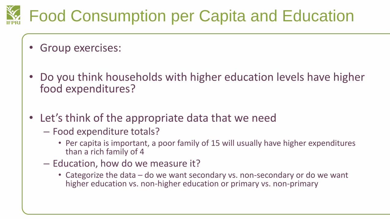
• Group exercises:

• Do you think households with higher education levels have higher food expenditures?

• Let’s think of the appropriate data that we need– Food expenditure totals?

• Per capita is important, a poor family of 15 will usually have higher expenditures than a rich family of 4

– Education, how do we measure it?• Categorize the data – do we want secondary vs. non-secondary or do we want

higher education vs. non-higher education or primary vs. non-primary

Solution

Solution

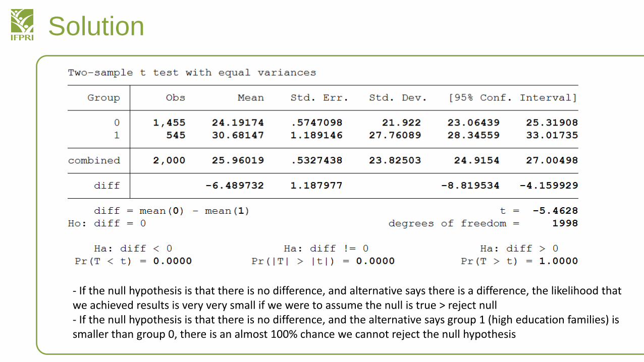
- If the null hypothesis is that there is no difference, and alternative says there is a difference, the likelihood that we achieved results is very very small if we were to assume the null is true > reject null- If the null hypothesis is that there is no difference, and the alternative says group 1 (high education families) is smaller than group 0, there is an almost 100% chance we cannot reject the null hypothesis

Econometrics Using Stata - ReSAKSS Asia · Introduction to Stata • What is Stata? –A computer...

Documents

Transcript of Econometrics Using Stata - ReSAKSS Asia · Introduction to Stata • What is Stata? –A computer...