Econometrics Regression Analysis with Time Series Datadocentes.fe.unl.pt/~azevedoj/Web...
21
Basics Assumptions Variance Trending Seasonality Further Issues Econometrics Regression Analysis with Time Series Data Jo˜ ao Valle e Azevedo Faculdade de Economia Universidade Nova de Lisboa Spring Semester Jo˜ ao Valle e Azevedo (FEUNL) Econometrics Lisbon, May 2011 1 / 21
Transcript of Econometrics Regression Analysis with Time Series Datadocentes.fe.unl.pt/~azevedoj/Web...
Basics Assumptions Variance Trending Seasonality Further Issues
EconometricsRegression Analysis with Time Series Data
Joao Valle e Azevedo
Faculdade de EconomiaUniversidade Nova de Lisboa
Spring Semester
Joao Valle e Azevedo (FEUNL) Econometrics Lisbon, May 2011 1 / 21
Basics Assumptions Variance Trending Seasonality Further Issues
Time Series Analysis
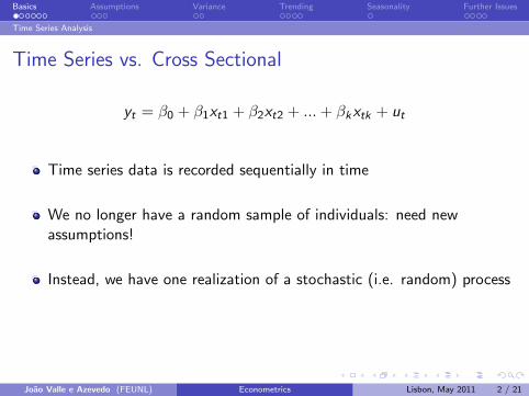
Time Series vs. Cross Sectional
yt = β0 + β1xt1 + β2xt2 + ...+ βkxtk + ut
Time series data is recorded sequentially in time
We no longer have a random sample of individuals: need newassumptions!
Instead, we have one realization of a stochastic (i.e. random) process
Joao Valle e Azevedo (FEUNL) Econometrics Lisbon, May 2011 2 / 21
Basics Assumptions Variance Trending Seasonality Further Issues
Time Series Analysis
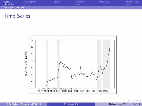
Time Series
Oil
pri
ces
($ p
erb
arre
l)
Joao Valle e Azevedo (FEUNL) Econometrics Lisbon, May 2011 3 / 21

Basics Assumptions Variance Trending Seasonality Further Issues
Time Series Analysis
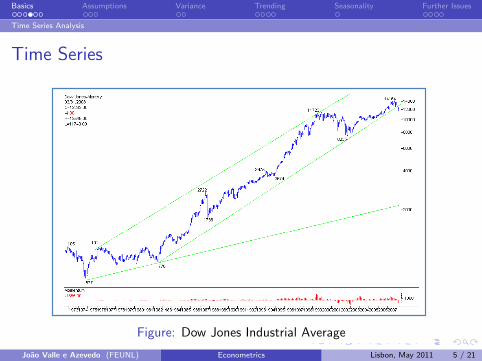
Time Series
Figure: Unemployment Rate: U.S. and EuropeJoao Valle e Azevedo (FEUNL) Econometrics Lisbon, May 2011 4 / 21
Basics Assumptions Variance Trending Seasonality Further Issues
Time Series Analysis
Time Series
Figure: Dow Jones Industrial Average
Joao Valle e Azevedo (FEUNL) Econometrics Lisbon, May 2011 5 / 21
Basics Assumptions Variance Trending Seasonality Further Issues
Time Series Analysis
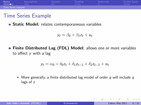
Time Series Example
Static Model: relates contemporaneous variables
yt = β0 + β1zt + ut
Finite Distributed Lag (FDL) Model: allows one or more variablesto affect y with a lag
yt = α0 + δ0zt + δ1zt−1 + δ2zt−2 + ut
I More generally, a finite distributed lag model of order q will include qlags of z
Joao Valle e Azevedo (FEUNL) Econometrics Lisbon, May 2011 6 / 21
Basics Assumptions Variance Trending Seasonality Further Issues
Time Series Analysis
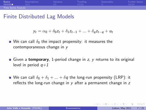
Finite Distributed Lag Models
yt = α0 + δ0zt + δ1zt−1 + ...+ δqzt−q + ut
We can call δ0 the impact propensity: it measures thecontemporaneous change in y
Given a temporary, 1-period change in z, y returns to its originallevel in period q+1
We can call δ0 + δ1 + ...+ δq the long-run propensity (LRP): itreflects the long-run change in y after a permanent change in z
Joao Valle e Azevedo (FEUNL) Econometrics Lisbon, May 2011 7 / 21
Basics Assumptions Variance Trending Seasonality Further Issues
Time Series Analysis
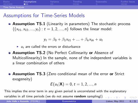
Assumptions for Time-Series Models
Assumption TS.1 (Linearity in parameters) The stochastic process{(xt1, xt2, ..., yt) : t = 1, 2, ..., n} follows the linear model:
yt = β0 + β1xt1 + ...+ βkxtk + ut
I ut are called the errors or disturbance
Assumption TS.2 (No Perfect Collinearity or Absence ofMulticollinearity) In the sample, none of the independent variables isa linear combination of others
Assumption TS.3 (Zero conditional mean of the error or Strictexogeneity)
E (ut |X) = 0, t = 1, 2, ..., n
This implies the error term in any given period is uncorrelated with the explanatory
variables in all time periods (we do not assume random sampling!)
Joao Valle e Azevedo (FEUNL) Econometrics Lisbon, May 2011 8 / 21

Basics Assumptions Variance Trending Seasonality Further Issues
Time Series Analysis
Unbiasedness of OLS
Under TS.1 through TS.3, OLS estimators are Unbiased conditional on X,and therefore unconditionally
E (ut |X) = 0, t = 1, 2, ..., n is a very strong assumption, often not verified
Suppose: CrimeRatet = β0 + β1PolicePerCapitat + ut in a given cityI u would need to be uncorrelated with current, past and future values of
PolicePerCapita. We can accept u is uncorrelated with current andpast values of the regressor. But clearly, an increase in u today is likelyto lead politicians to increase PolicePerCapita in the future! TS.3 fails!
Suppose: FarmYieldt = β0 + β1Labort + β2Rainfallt + ut for a givenfarm
I u would need to be uncorrelated with current, past and future values ofLabor. But maybe if last year’s u was low (some plague) the farmerwill not be able to hire as many workers next year. Ok with Rainfall, itwill most likely not affect u
Joao Valle e Azevedo (FEUNL) Econometrics Lisbon, May 2011 9 / 21

Basics Assumptions Variance Trending Seasonality Further Issues
Time Series Analysis
Unbiasedness of OLS (Cont.)
We do not worry if u is correlated with past regressors because wecan easily solve this problem: just include past regressors, use adistributed lag model
But we cannot have u influencing in any way future regressors! (atleast to guarantee unbiasedness)
Omitted variable bias can be analyzed in the same way as for across-section
An alternative assumption, closer to the cross-sectional case is:E (ut |xt) = 0. We would say the x ’s are contemporaneouslyexogenous. Contemporaneous exogeneity will only be sufficient inlarge samples
Joao Valle e Azevedo (FEUNL) Econometrics Lisbon, May 2011 10 / 21

Basics Assumptions Variance Trending Seasonality Further Issues
Time Series Analysis
Variance of OLS Estimators
We need to add an assumption of homoskedasticity in order to be able toderive variances
Assumption TS.4 (Homoskedasticity)
Var(ut |xt) = σ2 for t = 1, 2, ..., n(Compare to TS.4)
I Unlikely to hold in the model:
T − billRatest = β0 + β1Inflationt + β2Deficitt
Assumption TS.5 (No Serial Correlation)
Corr(ut , us |X) = Corr(ut , us) = 0 for t 6= s
The independent variables can be correlated across time!
Joao Valle e Azevedo (FEUNL) Econometrics Lisbon, May 2011 11 / 21
Basics Assumptions Variance Trending Seasonality Further Issues
Time Series Analysis
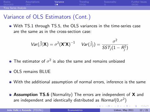
Variance of OLS Estimators (Cont.)
With TS.1 through TS.5, the OLS variances in the time-series caseare the same as in the cross-section case:
Var(β|X) = σ2(X′X)−1
Var(βj) =σ2
SSTj(1− R2j )
The estimator of σ2 is also the same and remains unbiased
OLS remains BLUE
With the additional assumption of normal errors, inference is the same
Assumption TS.6 (Normality) The errors are independent of X andare independent and identically distributed as Normal(0,σ2)
Joao Valle e Azevedo (FEUNL) Econometrics Lisbon, May 2011 12 / 21

Basics Assumptions Variance Trending Seasonality Further Issues
Time Series Analysis
Time Series with Trends
Economic time series often have a trendIf two series are trending together, we can’t assume that the relationis causalWe must always control for unobserved factors that can cause thetrends. Otherwise we have a spurious regression problem
Joao Valle e Azevedo (FEUNL) Econometrics Lisbon, May 2011 13 / 21

Basics Assumptions Variance Trending Seasonality Further Issues
Time Series Analysis
Models for Trends
One possible control is a linear trend
yt = α0 + α1t + et , t = 1, 2, ...
Another possibility is an exponential trend
log(yt) = α0 + α1t + et , t = 1, 2, ...
I where α1 is approx. the average growth rate of ylog(yt)− log(yt−1) ≈ (yt − yt−1)/yt−1
Or quadratic trend
yt = α0 + α1t + α2t2 + et , t = 1, 2, ...
Joao Valle e Azevedo (FEUNL) Econometrics Lisbon, May 2011 14 / 21

Basics Assumptions Variance Trending Seasonality Further Issues
Time Series Analysis
Adding trends in a regression
We should add a trend (usually linear) to the model if either thedependent variable or the independent variables are trending
yt = β0 + β1xt1 + β2xt2 + ...+ βkt + ut
If Assumptions TS.1 to TS.3 hold in this model, leaving the trend outwould in general lead to biased estimates of the remainingparameters, specially if the other regressors are trending
Adding a linear trend term to a regression is the same thing as using”detrended” series in a regression
Detrending a series involves regressing each variable in the model on tand a constant. The residuals form the detrended series
Then perform the regression with detrended variables (don’t needintercept, it will equal 0). It will give exactly the same estimates asthe regression above
Joao Valle e Azevedo (FEUNL) Econometrics Lisbon, May 2011 15 / 21

Basics Assumptions Variance Trending Seasonality Further Issues
Time Series Analysis
R2 with trending data
Time-series regressions with trends tend to have a very high R2
Should therefore look at the R2 from the regression with detrendeddata
This R2 better reflects how well the xt ’s explain yt
Can also use an adjusted R2 from the regression with detrended data
Joao Valle e Azevedo (FEUNL) Econometrics Lisbon, May 2011 16 / 21

Basics Assumptions Variance Trending Seasonality Further Issues
Time Series Analysis
Seasonality
Often time-series data exhibits seasonal behaviorSeasonality should be corrected by, e.g., regressing each of theseasonal variables on a set of seasonal dummiesCan seasonally adjust before running the regression (take the residualsfrom the previous regression)Should look at R-squared only on adjusted data (as for trends)
Beer
consumption
Joao Valle e Azevedo (FEUNL) Econometrics Lisbon, May 2011 17 / 21

Basics Assumptions Variance Trending Seasonality Further Issues
Time Series Analysis
Important types of Stochastic Processes
A stochastic process is stationary if for every collection of timeindices 1 ≤ t1 < ... < tm the joint distribution of (xt1, ..., xtm) is thesame as that of (xt1+h, ...xtm+h) for h ≥ 1
Otherwise the process is said to be nonstationary
Stationarity implies that the xt ’s are identically distributed and thatthe nature of any correlation between adjacent terms is the sameacross all periods
Joao Valle e Azevedo (FEUNL) Econometrics Lisbon, May 2011 18 / 21
Basics Assumptions Variance Trending Seasonality Further Issues
Time Series Analysis
Covariance Stationary and Weakly Dependent Processes
A stochastic process is covariance stationary if E (xt) is constant,Var(xt) is constant and for any t, h ≥ 1, Cov(xt , xt+h) depends onlyon h and not on t
A stationary time series is weakly dependent if xt and xt+h are”almost independent” as h increases
If for a covariance stationary process Corr(xt , xt+h)→ 0 as h→∞,we say this covariance stationary process is weakly dependent
Need weak dependence to use Laws of Large Numbers and CentralLimit Theorems
Joao Valle e Azevedo (FEUNL) Econometrics Lisbon, May 2011 19 / 21

Basics Assumptions Variance Trending Seasonality Further Issues
Time Series Analysis
An MA(1) Process
A moving average process of order one [MA(1)] satisfies:
yt = et + α1et−1, t = 1, 2, ...
where et is an i.i.d. sequence with mean 0 and variance σ2e
This is a stationary, weakly dependent sequence as y ’s 1 period apartare correlated, but 2 periods (and further) apart are not
Joao Valle e Azevedo (FEUNL) Econometrics Lisbon, May 2011 20 / 21
Basics Assumptions Variance Trending Seasonality Further Issues
Time Series Analysis
An AR(1) Process
An autoregressive process of order one [AR(1)] satisfies:
yt = ρyt−1 + et , t = 1, 2, ...
where et is an i.i.d. sequence with mean 0 and variance σ2e
For this process to be weakly dependent, it must be the case that|ρ| < 1
Corr(yt , yt+h) =Cov(yt , yt+h)
σyσy= ρh1
I which becomes small as h increases (check the derivation!)
Joao Valle e Azevedo (FEUNL) Econometrics Lisbon, May 2011 21 / 21