Econometric ModelingEconometric ModelingThrough EViews and Through EViews and

EXCELEXCEL

The Overview

Running an Ordinary Least Squares

Regression and Interpreting the

Statistics

Estimating the Consumption Function

C% = F(Y%)

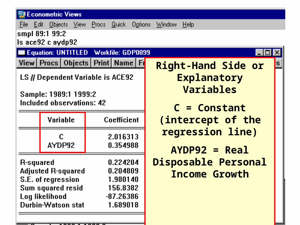
Right-Hand Side or Explanatory Variables

C = Constant (intercept of the regression line)

AYDP92 = Real Disposable Personal Income Growth

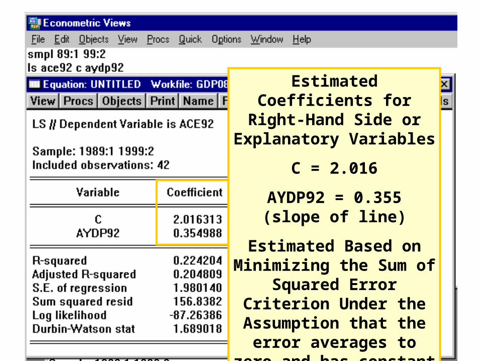
Estimated Coefficients for Right-Hand Side or

Explanatory Variables

C = 2.016

AYDP92 = 0.355(slope of line)

Estimated Based on Minimizing the Sum of

Squared Error Criterion Under the Assumption that the error averages to zero

and has constant variance.

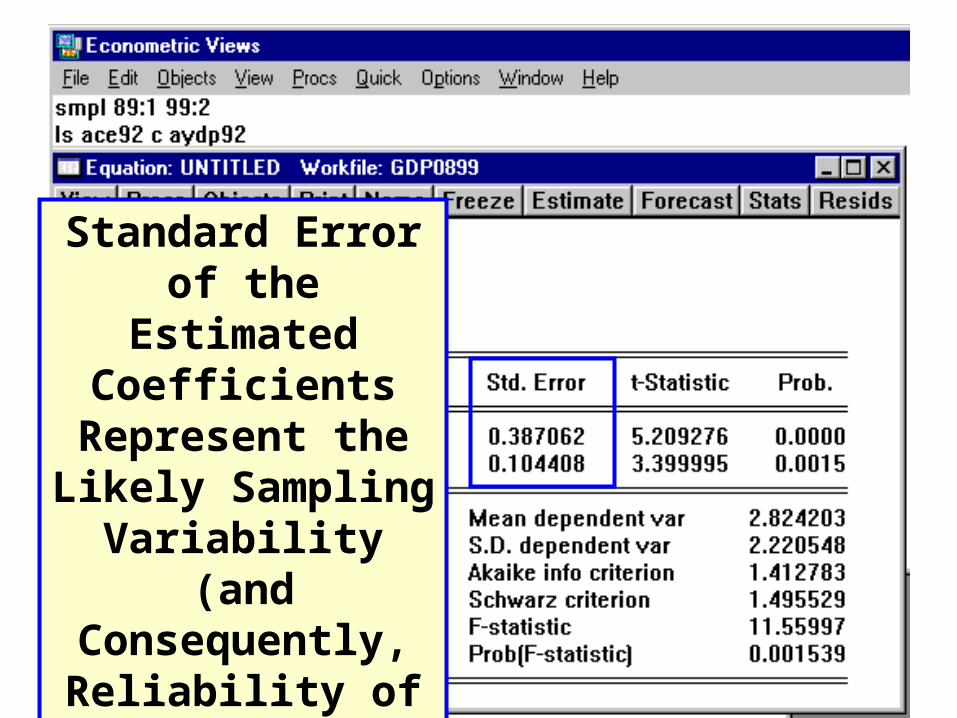
Standard Error of the Estimated Coefficients

Represent the Likely Sampling Variability (and Consequently,

Reliability of the Estimate).

T-Statistics

Each t-statistic provides a test of the hypothesis that the variable is zero or irrelevant (that is, contributes nothing to explaining the dependent variable).

The t-stat is the estimated coefficient divided by the standard error.

A t-stat whose absolute value is greater than 2 suggests that the

explanatory variable is statistically different from zero (that is, it is

relevant) at a 95% confidence interval.

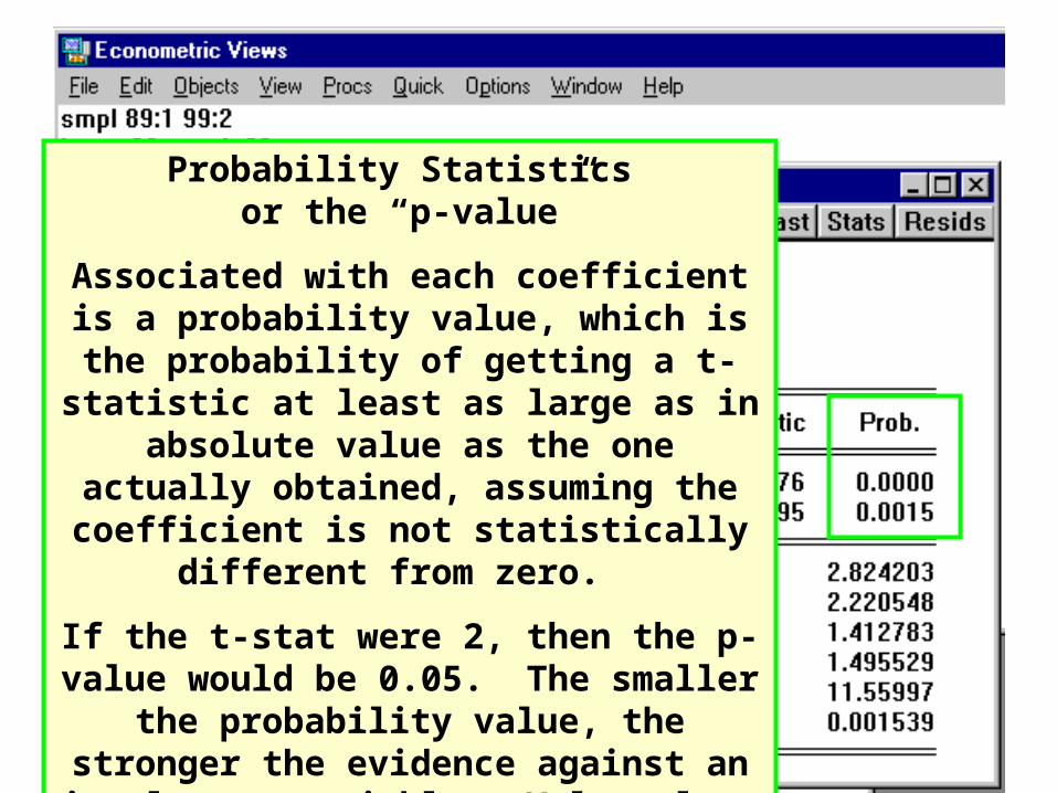
Probability Statistics or the “p-value”

Associated with each coefficient is a probability value, which is the probability of

getting a t-statistic at least as large as in absolute value as the one actually obtained, assuming the coefficient is not statistically

different from zero.

If the t-stat were 2, then the p-value would be 0.05. The smaller the probability value, the stronger the evidence against an irrelevant

variable. Values less than 0.1 are considered a strong evidence against an irrelevant variable.

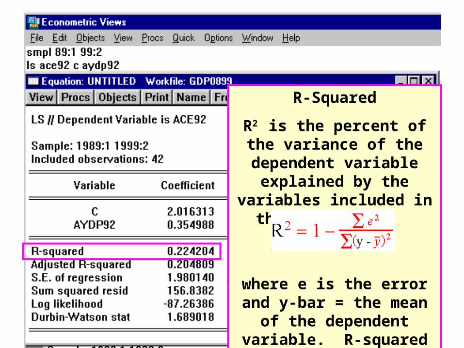
R-Squared

R2 is the percent of the variance of the dependent variable explained by the variables included in the

regression.

where e is the error and y-bar = the mean of the dependent variable. R-squared ranges

between zero and one.

R-Squared Adjusted

The Adjusted R-squared is interpreted the same as R-squared but the formula

incorporates adjustment for degrees of freedom used in

estimating the model.

As long as there is more than one right-hand-side variable (including the constant),

Adjusted R-squared will be less than R-squared.

Standard Error of Regression

where T is the number of observations and k is the degrees of

freedom (number variables).

This is a measure of dispersion and often is compared to the mean of

the dependent variable. The smaller the standard error is

relative to the mean of the dependent variable the better (and

the higher the R-squared).

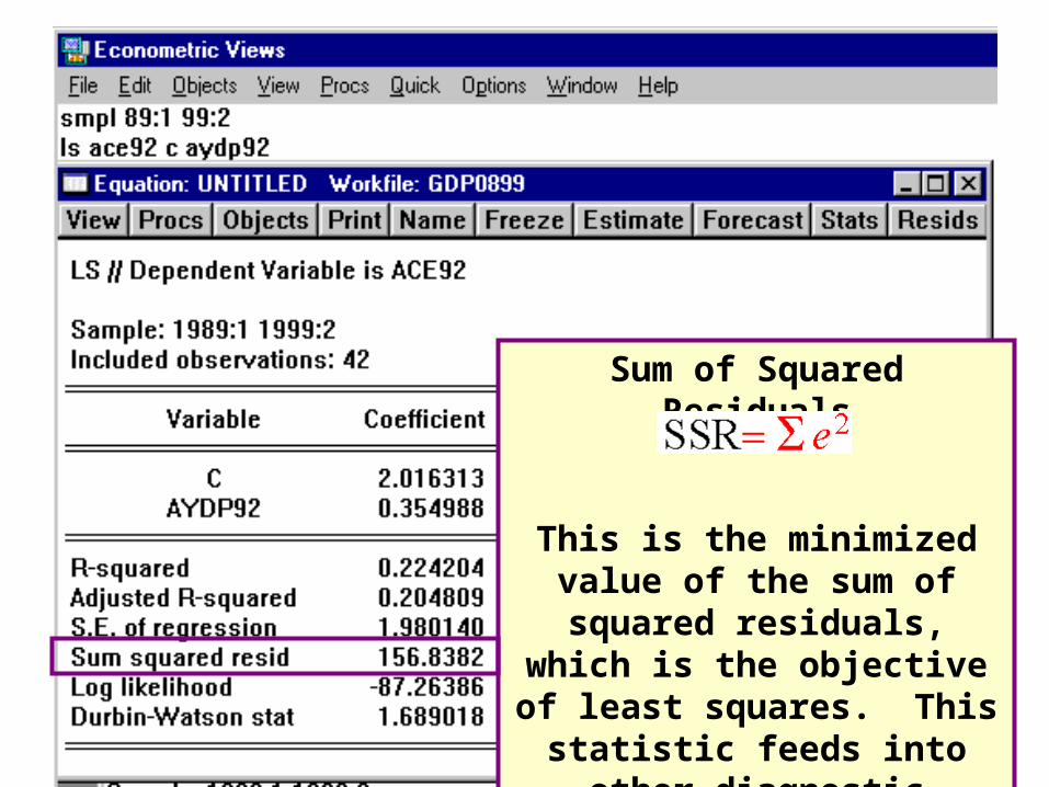
Sum of Squared Residuals

This is the minimized value of the sum of squared residuals, which is the objective of least

squares. This statistic feeds into other diagnostic measures and in

isolation is not very useful.

Log Likelihood

This figure is not used directly. However, an alternative estimation strategy is to maximize the likelihood

function to find parameter estimates. For normally

distributed errors, maximizing the likelihood function is

equivalent to the least square estimates derived from

minimizing sum of the squared error.

Durbin-Watson Statistic

The D-W stat tests for correlation over time in the errors. If errors are not correlated, they are not forecastable. However, when errors are correlated than the

overall forecast can be improved by forecasting those errors.

If no first-order serial correlation in the errors exist, then the D-W

stat = 2.0. Roughly, a D-W stat of less than 1.5 implies evidence of

positive serial correction and over 2.5 implies negative serial

correction.

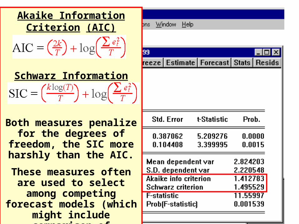
Akaike Information Criterion (AIC) Statistic

Schwarz Information Criterion (SIC)

Both measures penalize for the degrees of freedom, the SIC more harshly than the AIC.

These measures often are used to select among competing

forecast models (which might include comparison of different lag structures). The lower the AIC or SIC the better relative

to a competing model.

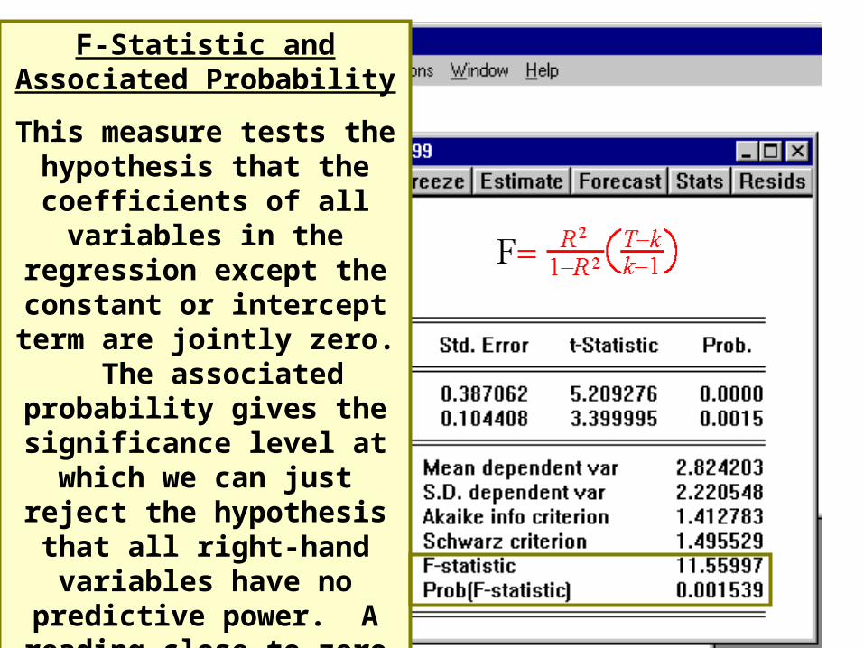
F-Statistic and Associated Probability

This measure tests the hypothesis that the coefficients

of all variables in the regression except the constant or intercept

term are jointly zero. The associated probability gives the significance level at which we can just reject the hypothesis that all right-hand variables have no predictive power. A

reading close to zero allows for rejection of hypothesis (accept

the implication that there is explanatory power).

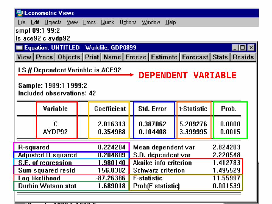
DEPENDENT VARIABLE

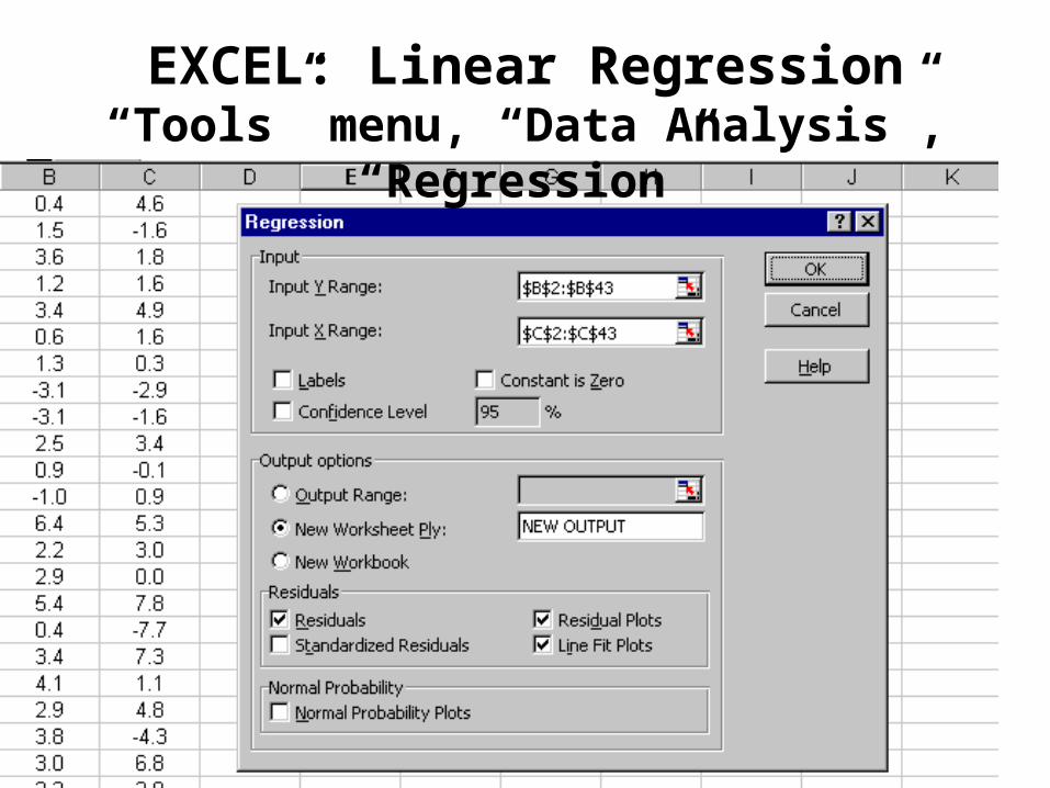
EXCEL: Linear Regression“Tools” menu, “Data Analysis”, “Regression”

The EXCEL Regression Output

Although the Battery of

Statistics are More Limited

Than from EVIEWS, Those Not Shown in

EXCEL Can be Calculated.

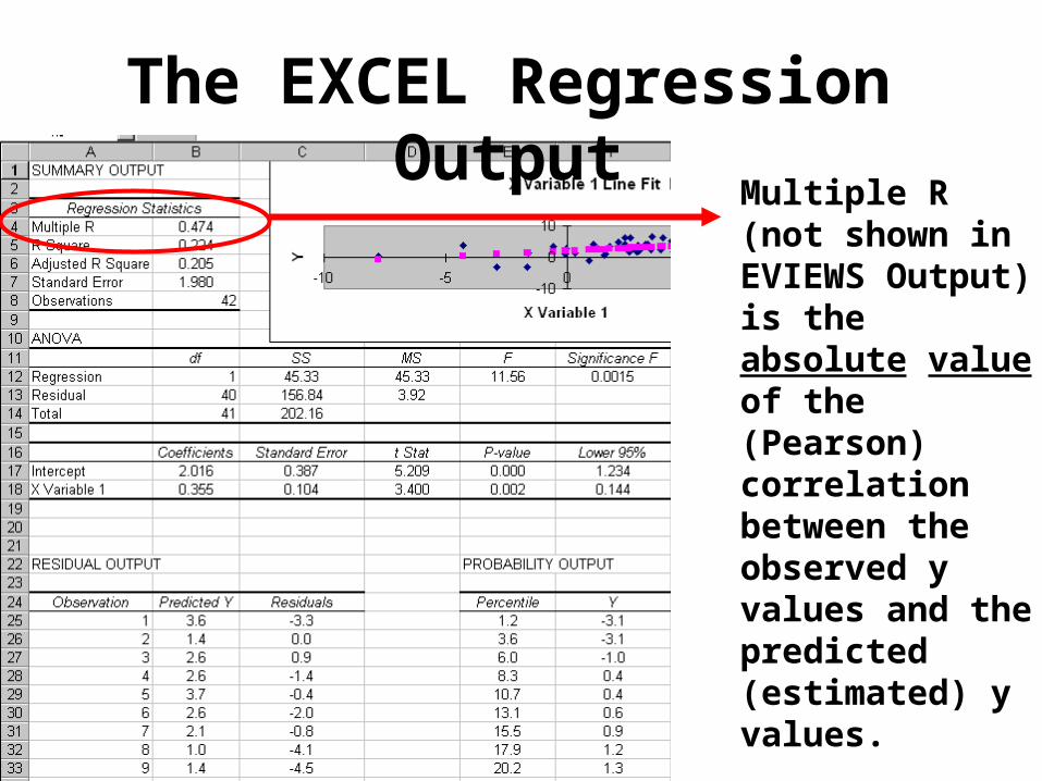
The EXCEL Regression Output

Multiple R (not shown in EVIEWS Output) is the absolute value of the (Pearson) correlation between the observed y values and the predicted (estimated) y values.

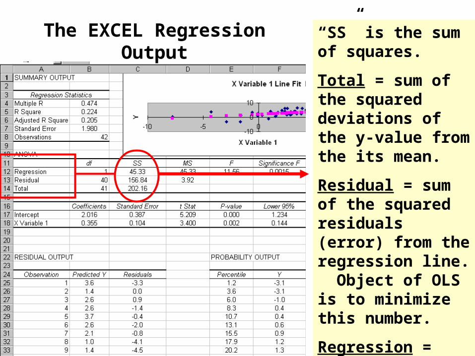
The EXCEL Regression Output “SS” is the sum of squares.

Total = sum of the squared deviations of the y-value from the its mean.

Residual = sum of the squared residuals (error) from the regression line. Object of OLS is to minimize this number.

Regression = Total - Residual. This represent amount of variance “explained.”

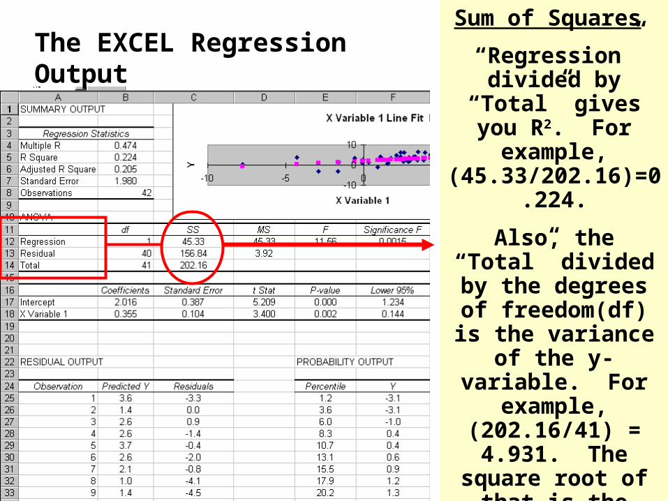
The EXCEL Regression OutputSum of Squares

“Regression” divided by “Total” gives you

R2. For example, (45.33/202.16)=0.224.

Also, the “Total” divided by the degrees of freedom(df) is the

variance of the y-variable. For

example, (202.16/41) = 4.931. The square root of that is the

standard deviation of the y-variable

(dependent variable) = 2.22 (percentage

points in this example).

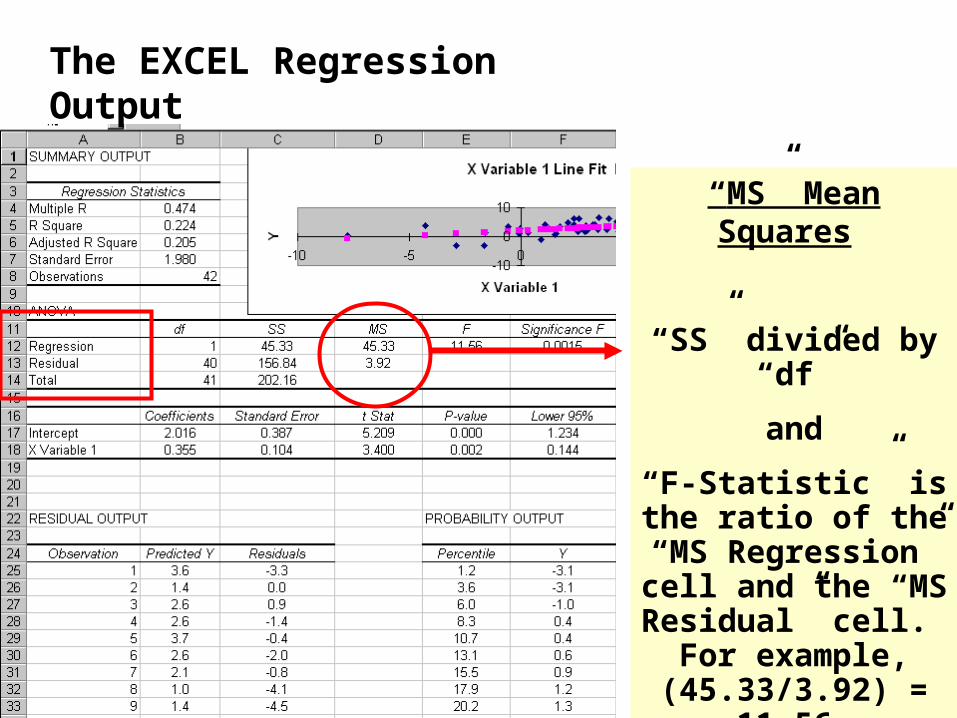
The EXCEL Regression Output

“MS” Mean Squares

“SS” divided by “df”

and

“F-Statistic” is the ratio of the “MS

Regression” cell and the “MS Residual” cell. For example,

(45.33/3.92) = 11.56.

The Five Assumptions Underlying the Classical Linear or Ordinary Least-Squares (OLS) Regression

Model for the Bivariate (y = a+bx) and the Multivariate

(y= a+bx1+cx2+dx3+…+nxn) Cases

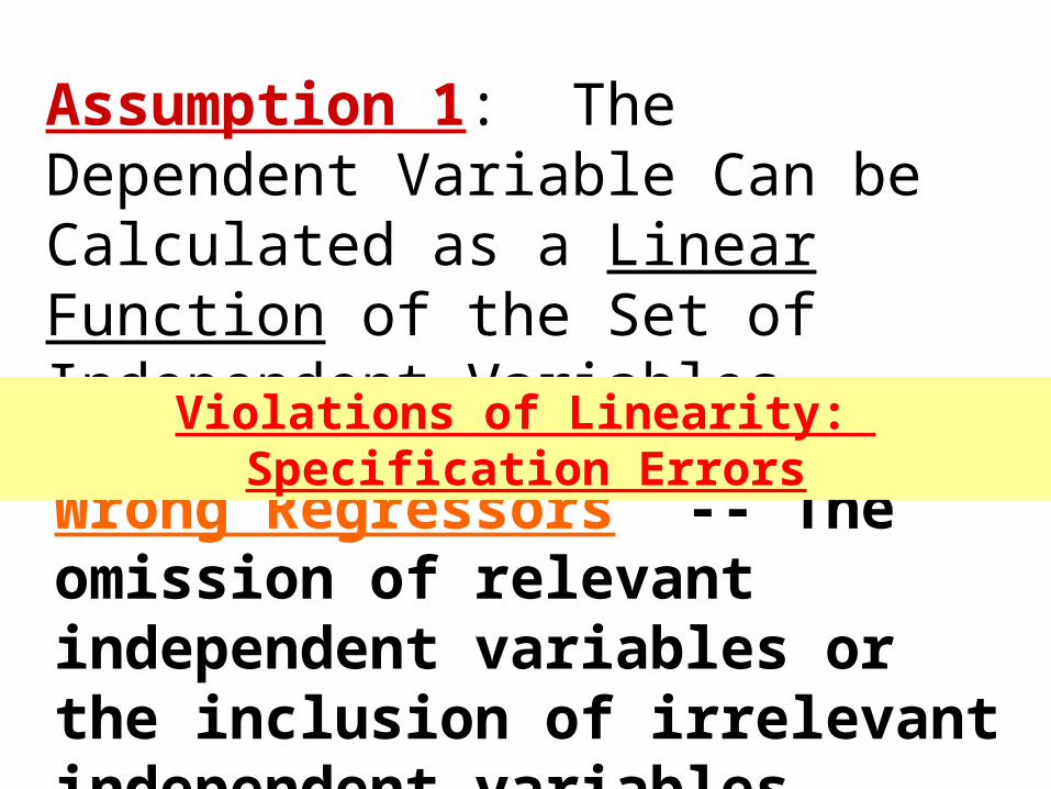
Assumption 1: The Dependent Variable Can be Calculated as a Linear Function of the Set of Independent Variables, Plus the Error Term.

Wrong Regressors -- The omission of relevant independent variables or the inclusion of irrelevant independent variables.

Violations of Linearity: Specification Errors

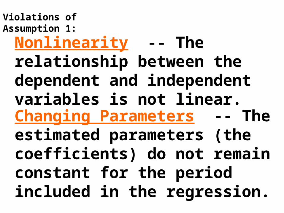
Changing Parameters -- The estimated parameters (the coefficients) do not remain constant for the period included in the regression.

Nonlinearity -- The relationship between the dependent and independent variables is not linear.

Violations of Assumption 1:

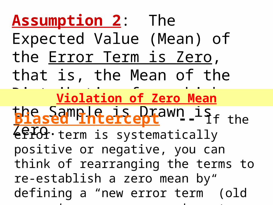
Assumption 2: The Expected Value (Mean) of the Error Term is Zero, that is, the Mean of the Distribution from which the Sample is Drawn is Zero.

Violation of Zero Mean

Biased Intercept -- If the error term is systematically positive or negative, you can think of rearranging the terms to re-establish a zero mean by defining a “new error term” (old error term = new error term + bias). Then the new constant term will equal old constant term + bias.

Assumption 3: The Error Terms have the Same Variance (homoskedasticity) and are not correlated with each other.

Violation of Uncorrelated Constant Variance

Heteroskedasticity -- The error terms do not have constant variance.

Autocorrelated Errors -- The error terms are correlated with each other.

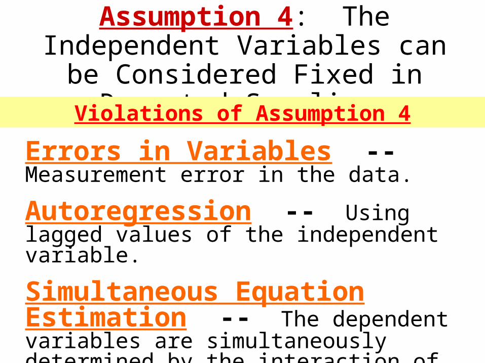
Assumption 4: The Independent Variables can be Considered Fixed in

Repeated Sampling.Violations of Assumption 4

Errors in Variables -- Measurement error in the data.

Autoregression -- Using lagged values of the independent variable.

Simultaneous Equation Estimation -- The dependent variables are simultaneously determined by the interaction of other relationships.

Assumption 5: The Number of Observations is Greater than the

Number of Independent Variables and there is No Exact Linear Relationship Between the Independent Variables.

Violation of Assumption 5

Multicollinearity -- Two or more independent variables are approximately linearly related in the sample period.

Popularity of OLS

1. Computational Convenience.

2. Ease of Interpretation.

3. The OLS estimates of the coefficients will the BEST LINEAR UNBIASED

ESTIMATES (BLUE) of the true coefficients.

Extensions of OLS are generally to Handle Violations

of These Assumptions

Once You have Estimated Your Equations and Developed Your Model, Then the Next Step is to

Simulate the Model.

A System of Equations Can Be Solved Using the Gauss-Seidel

Method

You Do Not Need to Know too Much About This Since

it is Built Into Either EXCEL (if you turn the option on) or EViews.

Forecast Simulation Topics

• The Gauss-Seidel Method.

• EXCEL Simulation Model.

Look at GAUSSSEI.XLSWhich is Found on Website

Demonstrates the Concept of Solving a Set of

Simulataneous Equations.

Turn Iteration Option On to Solve Model