Econometric Analysis of Health Data

Econometric Analysis ofHealth Data

Econometric Analysis of Health DataEdited by Andrew Jones, Owen O’DonnellCopyright © 2002 John Wiley & Sons Ltd

ISBNs: 0-470-84145-1 (Hardback); 0-470-84631-3 (Electronic)

Econometric Analysis ofHealth Data

Edited by

Andrew M. JonesDepartment of Economics and Related Studies,University of York,UK

and

Owen O’DonnellDepartment of Balkan, Slavic and Oriental Studies,University of Macdeonia,

Thessaloniki, Greece



Copyright© 2002 by John Wiley & Sons, Ltd.,Baffins Lane, Chichester,West Sussex PO19 1UD, UK

National 01243 779777International (�44) 1243 779777

e-mail (for orders and customer service enquiries): [email protected] our Home Page on: http://www.wiley.co.uk

All Rights Reserved. No part of this publication may be reproduced, stored in a retrievalsystem, or transmitted, in any form or by any means, electronic, mechanical, photocopying,recording, scanning or otherwise, except under the terms of the Copyright, Designs and Patents Act1988 or under the terms of a licence issued by the Copyright Licensing Agency Ltd, 90 Tottenham CourtRoad, LondonW1P 0LP, without the permission in writing of the publisher.

OtherWiley Editorial Offices

JohnWiley & Sons, Inc., 605 Third Avenue,New York, NY 10158-0012, USA

Wiley-VCH Verlag GmbH, Pappelallee 3,D-69469 Weinheim, Germany

JohnWiley & Sons (Australia) Ltd, 33 Park Road, Milton,Queensland 4064, Australia

JohnWiley & Sons (Asia) Pte Ltd, 2 Clementi Loop �02-01,Jin Xing Distripark, Singapore 129809

JohnWiley & Sons (Canada) Ltd, 22 Worcester Road,Rexdale, Ontario M9W 1L1, Canada

British Library Cataloguing in Publication Data

A catalogue record for this book is available from the British Library

ISBN 0-470-84145-1

Typeset in 9/11pt Times by Vision Typesetting, ManchesterPrinted and bound in Great Britain by Antony Rowe Ltd, ChippenhamThis book is printed on acid-free paper responsibly manufactured from sustainable forestry,in which at least two trees are planted for each one used for paper production.



Dedication

As secretary for the EuropeanWorkshop series, Barbara Olive has been largely responsible forthe smooth running of the preparations for the meetings. This dedication is a token of ourgratitude. We wish her great happiness in her retirement.



Contents

List of Contributors . . . . . . . . . . . . . . . . . . . . . . . . . . ix

Preface . . . . . . . . . . . . . . . . . . . . . . . . . . . . . . . . . . . xi

Introduction . . . . . . . . . . . . . . . . . . . . . . . . . . . . . . . . 1AndrewM. Jones and Owen O’Donnell

I: Latent Variables and Selection Problems

1 The demand for health: an empiricalreformulation of the Grossman model . . . . . . . . 15AdamWagstaff

2 Health, health care, and the environment:Econometric evidence from Germanmicro data . . . . . . . . . . . . . . . . . . . . . . . . . . . . 25Manfred Erbsland,Walter Riedand Volker Ulrich

3 Subjective health measures andstate-dependent reporting errors . . . . . . . . . . . . . 37Marcel Kerkhofs and Maarten Lindeboom

4 The effect of smoking on health using asequential self-selection model . . . . . . . . . . . . . . 51Kajal Lahiri and Jae G. Song

II: Count Data and Survival Analysis

5 A comparison of alternative models ofprescription drug utilization . . . . . . . . . . . . . . . . 73Paul V. Grootendorst

6 Estimates of the use and costs ofbehavioural health care: a comparison ofstandard and finite mixture models . . . . . . . . . . . 87Partha Deb and Ann M.Holmes

7 Latent class versus two-part models inthe demand for physician services acrossthe European Union . . . . . . . . . . . . . . . . . . . . . 101Sergi Jimenez-Martın, Jose M. Labeaga,Maite Martınez-Granado

8 Proportional treatment effects forcount response panel data: effects ofbinary exercise on health care demand . . . . . . . 117Myoung-jae Lee and Satoru Kobayashi

9 Estimating surgical volume–outcomerelationships applying survival models: accountingfor frailty and hospital fixed effects . . . . . . . . . . 133Barton H.Hamilton and Vivian H.Ho

III: Flexible and Semiparametric Estimators

10 Individual cigarette consumption andaddiction: a flexible limited dependentvariable approach . . . . . . . . . . . . . . . . . . . . . . 147Steven T. Yen and AndrewM. Jones

11 Identifying demand for healthresources using waiting timesinformation . . . . . . . . . . . . . . . . . . . . . . . . . . . 159Richard Blundell and FrankWindmeijer

12 Non- and semi-parametric estimationof age and time heterogeneity in repeatedcross-sections: an application to self-reportedmorbidity and general practitioner utilization . . 167David Parkin,Nigel Rice and Matthew Sutton

IV: Classical and Simulation Methodsfor Panel Data

13 Unobserved heterogeneity and censoringin the demand for health care . . . . . . . . . . . . . . 181Angel Lopez-Nicolas

14 A discrete random effects probit modelwith application to the demand forpreventive care . . . . . . . . . . . . . . . . . . . . . . . . . 189Partha Deb

15 The use of long-term care services bythe Dutch elderly . . . . . . . . . . . . . . . . . . . . . . . 201France Portrait,Maarten Lindeboomand Dorly Deeg

16 HMO selection and medical care costs:Bayesian MCMC estimation of a robustpanel data probit model with survival . . . . . . . . 217Barton H.Hamilton

Index . . . . . . . . . . . . . . . . . . . . . . . . . . . . . . . . . . . 229



Contributors

Richard Blundell University College London,Department of Economics, Gower Street, London,WC1E6BT,UK

Partha Deb Department of Economics, IndianaUniversity Purdue University, Indianapolis, 425University Boulevard, Indianapolis IN 46202,USA

Dorly Deeg Free University of Amsterdam,DeBoelelaan 1105, 1081HV Amsterdam, TheNetherlands

Manfred Erbsland Fachhochscule Neubrandenburg,Studiengang Pflege U Gesundh, 17041Neubrandenburg,Germany

Paul V. Grootendorst Centre for Evaluation ofMedicines, St Joseph’s Hospital,MarthaWing Room H-319, 50 Charlton Ave East, Hamilton Ontario, Canada L8N4A6

Barton H. Hamilton John M. Olin School of Business,Washington University in St Louis, Campus Box 1133,One Brookings Drive, St Louis MO 63130,USA

Vivian H. Ho Health Care Organization and Policy,Department of General Practice,University of AlabamaBirmingham, RPHB 330, 1530 3rd Ave. South,Birmingham, AL 35294-0022,USA

AnnM. Holmes 801 W. Michigan St., Room 4070,Spea-IUOUI, Indianapolis, IN 46202 5199,USA

Sergi Jimenez-Martın Department of Economics,Universidad Carlos III de Madrid, c/Madrid,126E-28903 Getafe,Madrid, Spain

AndrewM. Jones Department of Economics andRelated Studies,University of York,Heslington YorkYO10 5DD,UK

Marcel Kerkhofs Organisation of Labour MarketResearch, Tilburg University, PO Box 90153 5000 LETilberg, The Netherlands

Jose M. Labeaga Universidad Nacional De EducacionA Distancia, Facultad De CC. Economicas YEmpresariales, Departamento De Analisis Economico,Senda Del Rey, 11, 28040Madrid, Spain

Saturo Kobayashi Institute of Policy and PlanningSciences,University of Tsukuba, Tsukuba, Ibaraki305-8573, Japan

Kajal Lahiri Department of Economics,University ofAlbany: SUNY, 1400 Washington Avenue, Albany NY12222,USA

Myoung-jae Lee Department of Economics,Sungkyunkwan University, 3–53Myongryun-dony, Seoul110-745, South Korea

Maarten Lindeboom Department of Economics, VrijeUniversiteit,De Boelelaan 1105 1081HV Amsterdam,The Netherlands

Angel Lopez-Nicolas Universitat Pompen Fabra,Departmento de Economia Y Epresa CIRamon TriasFargas 25-27, 08005-Barcelona, Spain

Maite Martınez-Granado Department of Economics,Department of Psychiatry,Universidad Carlos III deMadrid, c/Madrid, 126.E-28903 Getafe,Madrid,Spain

Owen O’Donnell Department of Balkan, Slavic andOriental Studies,University of Macedonia, 156 EgnatiaStreet, Thessaloniki, 54006, Greece

David Parkin Department of Economics, CityUniversity,Northampton Square, London, EC1V 0HB,UK

France Portrait Faculty of Econometrics, VrijeUniversiteit,De Boelelaan 1105 1081HV Amsterdam,The Netherlands

Nigel Rice Centre for Health Economics,University ofYork,Heslington York YO1 5DD, UK



Walter Ried Department of Economics,University ofMannheim, Seminargbaude AS, B247, 68131Mannheim,Germany

Jae G. Song Department of Economics,University ofAlbany: SUNY, 1400 Washington Avenue, Albany NY12222,USA

Matthew Sutton Department of General Practice,University of Glasgow, 4 Lancaster Crescent, Glasgow,G42 0RR,UK

Volker Ulrich Ernst-Moritz-Arndt-UniversitatGreifswald, Rechts- und Staarswissenschaftliche Fakultat,Lehrstuhl fur Allgemeine Volkswirtschaftslehre, insb.Finanzwissenshaft, Postfach, 17487 Greifswald, Germany

FrankWindmeijer Institute for Fiscal Studies, 7Ridgemount Street, LondonWC1E 7AE,UK

AdamWagstaff Visiting Research Fellow,HumanDevelopment Network, Room G3-038, TheWorld Bank,1818H Street NW,Washington CD 20433,USA

Steven T. Yen Department of Agricultural Economics,308-DMorgan Hall, 2621Morgan Circle,University ofTennessee,Knoxville, TN 37996-4518,USA

x CONTRIBUTORS

Preface

The purpose of this book is to give readers convenientaccess to a collection of innovative applications ofeconometric methods to data on health and health care.The contributions are selected from papers presented atthe European Workshops on Econometrics and HealthEconomics which have been published in Health Econ-omics. The Workshops were established in York, withmeetings in 1992 and 1993. Since then they have takenplace annually, with locations in eight differentEuropean countries. Publication of the present volumemarks the tenth anniversary of the Workshop series, theoverall aim of which is to provide a forum for the devel-opment and dissemination of econometric methods inhealth economics. When the Workshops were first estab-lished, there were relatively few European researchersat the frontiers of quantitative research in the area.Advances in quantitative techniques and the increasedavailability of datasets and computing technology had

created the potential for large returns from attractingmore researchers into health econometrics. There are in-dications that these returns are now being reaped. Overthe years, there has been a steady rise in the quantityand general quality of submissions received for eachWorkshop.We would like to thank everyone who has par-

ticipated in the Workshop series, whether as an authoror a discussant, and all of those who have reviewed pa-pers for Health Economics. Our particular gratitude goesto the local organisers of the Workshops: Eddy vanDoorslaer (Antwerp, 1994), Lise Rochaix (Paris, 1995),Guillem Lopez-Casasnovas (Barcelona, 1996), Joa� o Per-eira (Lisbon, 1997), Unto Hakkinen and Miika Linna(Helsinki, 1998), Giacomo Pignataro and Ilde Rizzo(Catania, 1999) and Maarten Lindeboom and FrancePortrait (Amsterdam, 2000).



Index

activities of daily living indicators(ADL) 3

addictionsflexible limited dependent variables8—9, 147—57

smoking 8—9, 52, 60—9, 147—57withdrawal symptoms 148

ADL see activities of daily livingindicators

age issues 9—10, 17, 19—23, 30—6, 43—9,109—15, 195—8

elderly long-term care 11, 201—27exercises 121—31GP utilization 167—77hip fractures 133—44HMOs 220—7mental illness 91—9prescriptions 77—86smoking effects 53—69, 152—7surgical volume-outcomerelationships 138—44

AIC see Akaike information criteriaair pollution 2, 25—36Akaike information criteria (AIC) 90—9,

108, 194—8alcoholics

see also drinking habitsmental illness 91—9smoking 54—69

Andrews’ test 90—3arthritisexercises 121—31smoking 55—69

ATE see average treatment effectAustria 102—16average treatment effect (ATE) 6—7,

117—32

Bank of America 117Bayesian information criteria (BIC)

90—9, 108Bayesian Markov Chain Monte Carlo

estimation (MCMC) 11—12, 218—27behavioural health care, FMM/TPM

comparisons 87—99Belgium 102—16Berndt-Hall-Hall-Hausmann algorithm

(BHHH) 58

biases 4, 9, 37—49, 52—69, 77, 159—66BIC see Bayesian information criteriabinary exercise effects 6—7, 117—32binary responses 1, 10—12, 80—1, 101—4,

152bivariate smoothing 167—77blood pressure 190—8exercises 121—31smoking 55—69

Blundell, Richard 9, 159—66Box—Cox double hurdle model 8—9,

147—57British Family Expenditure Survey

(FES) 150—7British General Household Survey

(GHS) 9, 150—2, 167—77British Health and Lifestyle Survey

(HALS) 8—9, 148—57British Social Attitudes Survey

148Broyden-Fletcher-Goldfarb-Shanno

algorithm 90, 199

Canada 5, 73—86, 133—44cancers 53—4, 77, 123capitated payment structuresFMM/TPM comparisons 87—98HMO selection 217—18

censoring issues 1, 10—11, 181—8Center for Economic Research on

Retirement and Aging (CERRA)39—48

cessation issues, smoking 51, 58—69,147—57

CFES see Spanish Continuous FamilyExpenditure Survey

CHAMPS/VA 121, 123Charlson comorbidity index 135—44chi-squared tests 21—2children, emotional disorders 91cholesterol levels 55—69, 190—8Chow test 170—1chronic complaints 30—6, 51—69, 77—9,

102, 109—15, 121—31, 152—7, 220cigarettes see smokingclassical methods 1, 6—7, 10—12, 181—227Cobb-Douglas production function 29,

182

cohort effects 171—2community sizes 30—6competing risks 7—8conditional treatment effects, count

response panel data 118—20,125—31

consultations 19—23, 30—6continuous densities, FMM/TPM

comparisons 89—90, 98costs 217—27EU demands 101—16FMM/TPM comparisons 87—99hassle costs 159—66health lifestyles 117—32HMOs 217—27LCM/TPM comparisons 101—16Medicare costs 217—27opportunity costs 79reduction methods 117—32

count data 1, 4—8, 73—144cream-skim incentives 88, 96, 218—27cross-section data 167—77, 185—8panel data 118, 127—8smoking 148

cross-validation issues (CV) 108—15,169—77

Danish Health Study (DHS) 18—23Deb, Partha 5—6, 11, 87—99, 124,

189—200Deeg, Dorly 3—4, 201—16degrees of handicap 30—6demands 2—3, 6—12, 15—36, 88—116,

159—66, 181—8binary exercise effects 6—7, 117—32censoring issues 1, 10—11, 181—8EU 101—16gender issues 105—16income links 105—6preventive care 189—200waiting times 9, 159—66

demographic factors 205—15EU demands 115HMOs 219—27long-term care services 205—15mental illness 91—9prescriptions 77—86smoking 54—69, 152—7



demographic factors (cont.)specialists 115surgical volume-outcomerelationships 138—44

Denmark 18—23, 102—16depreciation effects, health stocks 2—3,

10—11, 15—36, 64, 181—8depressives 88DHS see Danish Health Studydiabetesexercises 121—31smoking 55—69

disabled persons 37—49, 152—7discharge transition intensities, surgical

volume-outcome relationships138—44

discrete densities, REP 189—200diseases 51—69, 121—31, 152—7, 220prescriptions 77—86smoking 51—69, 152—7

distributional assumptions 1, 8—10,147—77

double hurdle models 8—9, 147—57drinking habits

see also alcoholicshealth lifestyles 117mental illness 91—9smoking 54—69

drug abuse, mental illness 91—9duration models 7—8, 133—44dynamics 1, 2—4, 10—12, 15—23

early-retired groups 38—49ECHP see European Community

Household Paneleconometric analysis 1—12, 89—90education issues 16—23, 30—6, 41—3,

54—69, 109—18, 121—31, 205—15,220—7

elderly long-term care 11, 201—27emotional disorderschildren 91exercises 121—31

empirical reformulations, Grossmanmodel 2—3, 10—11, 15—23, 28—35,181—8

empirical sections, theoretical links 2,15—36

employment issues 3, 38—49, 54—69,78—86, 109—15, 217

exercises 121—31HMOs 217smoking 61—9, 152—7

endogeneity 1—2, 4, 37—49, 56—69, 117,159—66, 202, 207—8

environmental impacts 2—3, 18—23,25—36

Erbsland, Manfred 2—3, 25—36errors 1—3, 8, 11, 33—49, 56, 80, 90, 104,

147—57, 189—200, 205estimation issues 1—12, 20—6, 33—6, 43—9,

57—8, 83, 104, 134—44, 159—66,217—27

European Community Household Panel(ECHP) 102—16

European Union (EU) 6, 101—16see also individual countriesdemands 6, 101—16LCM/TPM comparisons 101—16

evaluations, treatment effects 6—7,117—32

exercises 7, 56—69, 117—32concepts 117—32proportional treatment effects 117—32

expenditures 1, 8—10, 27, 35, 73—99,182—8, 205—27

EU demands 101—16FMM/TPM comparisons 87—99health lifestyles 117—32HMOs 217—27LCM/TPM comparisons 101—16mortality links 217—27reduction methods 117—32

feesEU demands 101—16fee-for-service payments 6

FES see British Family ExpenditureSurvey

FIML see full information maximumlikelihood

finite mixture model (FMM) 5—6, 9,87—99, 198—9

advantages 88—9capitated rate-setting applications96

concepts 87—99mental illness 87—99results 91—9TPM comparisons 87—99

Finland 101fixed-effect panel estimators 123—31flexible estimators 1, 8—10, 147—77FMM see finite mixture modelformal long-term care services 202—15frailty issues 8, 133—44France 101full information maximum likelihood

(FIML) 2—4, 33—6, 54—69, 209

Gamma distributions 103—4gatekeepers, EU demands 6, 101—16Gauss-hermite quadrature 10gender issues 19—23, 30—6, 43—9, 54—69,

80—6, 121—31, 153—7, 195—8EU demands 105—16exercises 121—31GP utilization 167—77HMOs 220—7LCM 105—16long-term care services 205—15mental illness 91—9

specialists 105—16surgical volume-outcomerelationships 138—44

general practitioners (GPs)age issues 167—77EU demands 101—16LCM 101—16morbidity effects 173—7specialists 101—16visits 1, 4—8, 10—11, 19—23, 30—6, 83,89, 91—116, 120—32, 181—8

Germany 25—36, 102—16GHS see British General Household

SurveyGibbs sampling 11GMD doctors 38—9GMM estimator 10GoM see Grade of MembershipGPs see general practitionersGrade of Membership (GoM) 3—4,

202—15Greece 102—16Grootendorst, Paul V. 5—6, 73—86Grossman model 2—3, 10—11, 15—23,

25—36, 181—8alternative empirical formulation17—23, 28—36

concepts 15—23, 25—30discussion 22, 35—6empirical reformulations 2—3, 10—11,15—23, 28—35, 181—8

previous empirical work 16—17, 26—30

HALS see British Health and LifestyleSurvey

Hamilton, Barton H. 7—8, 11—12,133—44, 217—27

hassle costs, waiting times 159—66Hausman-type specification test 35—6,

125hazard rates 7—8hazardous work, smoking effects 61—9health lifestyles 117—32health maintenance organizations

(HMOs) 11—12, 217—27health measures 152—7health promotions, smoking 152Health and Retirement Survey (HRS)

41, 53—4, 117—32health status 102, 138—44, 152—7, 202—27long-term care services 202—15prescriptions 77—86

health stocks 2—3, 10—11, 15—36, 64, 115,181—8

heart disease 152—7, 220exercises 121—31smoking links 51—4, 152—7

Heckit estimator 9Heckman-Lee two-step method 54—8Heckman-Singer nonparametric

approaches 8, 134

230 ECONOMETRIC ANALYSIS OF HEALTH DATA

heterogeneity 4—11, 52—69, 83—9, 98,101—16, 133—44, 167—77, 181—8

heteroskedasticity 90—9prescriptions 81smoking effects 56—69

hip fractures 133—44HMOs see health maintenance

organizationsHo, Vivian H. 7—8, 133—44Holmes, Ann M. 5—6, 11, 87—99homoskedasticity 80—1, 84—5, 93, 96Hopkins symptom checklist (HSCL) 3,

39, 41—3hospitalsbeds 19—23, 30—6, 102, 109—15, 133—44days 120—44fixed effects 7—8, 133—44waiting times 9, 159—66

housing adaptations, long-term careservices 205—15

HRS see Health and Retirement SurveyHSCL see Hopkins symptom checklisthurdle models 89—99, 104, 147—57, 184

see also two-part modelsconcepts 89FMM comparisons 89—99

hypertension see blood pressure

ICD-9 see International Classification ofDiseases 9th Revision

income issues 19—23, 27—49, 55—69, 91,102, 105—16, 195—8, 205—15

EU demands 105—16exercises 121—31HMOs 220—7long-term care services 205—15prescriptions 77—86smoking effects 55—69, 152—7specialists 105—16surgical volume-outcomerelationships 138—44

influenza shots 190—8informal long-term care services 202—15initiation issues, smoking 51, 58—69insurance schemes 117, 121—31, 196disabled persons 37—49mental illness 91—9prescriptions 73, 77—86smoking effects 55—69

International Classification of Diseases9th Revision (ICD-9) 91—9

investments, health stocks 2—3, 10—11,15—36, 64, 181—8

Ireland 102—16Italy 102—16

Jimenez-Martin, Sergi 6, 101—16Jones, AndrewM. 1—12, 147—57

Kerkhofs, Marcel 3, 37—49Kobayashi, Saturo 6—7, 117—32

Kullback-Leibler information criteria90

Lahari, Kajal 4, 51—69LASA see Longitudinal Ageing Study

Amsterdamlatent class models (LCMs) 101—16concepts 101—16cross-validation issues 108—15disadvantages 105EU demands 101—16results 106—16

latent variables 1—4, 6, 11—12, 15—69,101—16, 124—5, 137, 217—27

see also unobservable...overview 1—4

LCMs see latent class modelsLDV model 11, 156, 181—8Lebeaga, Jose M. 101—16Lee, Myoung-jae 6—7, 117—32Legendre polynomials 43light exercises 7, 121—32likelihood ratio tests (LR) 81—6, 194—8limited dependent variables 8LINCS see linear covariance structuresLindeboom, Maarten 3, 37—49, 201—16linear covariance structures (LINCS) 33linear structural relationships (LISREL)

2, 20—3long-term care services 3—4, 11—12,

77—86, 201—27elderly needs 11, 201—27Netherlands 11, 201—16types 202—3

Longitudinal Ageing Study Amsterdam(LASA) 11, 201—16

longitudinal data 1, 4, 10—12, 105, 120,133—44, 201—16

Lopez-Nicolas, Angel 10—11, 181—8LR see likelihood ratio testslung diseases 121—31, 152—7Luxembourg 102—16

major affective disorders 88, 91—9,121—31

marginal treatment effects, countresponse panel data 118—20, 128—9

marital status 43—9, 55—69, 109—15, 118,121—31, 153—7

long-term care services 205—15smoking 153—7surgical volume-outcomerelationships 138—44

Martınez-Granado, Maite 101—16maximum likelihood estimates (ML) 8,

10—11, 20—3, 33—6, 43—9, 57—8, 90—9,102—16, 124—6, 185—8, 209, 210—16,218, 222

maximum simulated likelihood estimates(MSL) 11, 210—16

Mayo Clinic 51

MCMC see Bayesian Markov ChainMonte Carlo estimation

mean squared error (MSE) 76, 80measurement errors 37—49MED-ICHO database 134mental illnesses 87—99, 121—31MEPS see United States of America...method of moment estimator (MME)

124—31methodology concepts 1Michigan Survey Centre 41microeconometrics 1, 182—3MIMIC see multiple indicators multiple

causesminimum-ignorance estimators 33ML see maximum likelihood estimatesMME see method of moment estimatorMonte Carlo simulations 11—12, 57,

189—200, 218—27morbidity issues 135—44, 167—77mortality issues 7—8, 19, 38, 134—44,

208—27MSE see mean squared errorMSL see maximum simulated likelihood

estimatesmultidimensionality issues 3—4multiple indicators multiple causes

(MIMIC) 2—3, 18—23Mushkin, S.J. 25

Nadaraya-Watson estimator 9NB see negative binomial modelNBS see United States of America...negative binomial model (NB) 74—6,

80—6, 89—99, 101—16, 124—31Netherlands 11—12, 38—49, 102—16,

201—16networks, informal long-term care

services 205—15New Beneficiary Survey 11nicotine see smokingnoise pollution 2, 25—36nonlinear models 1, 10—11, 181—200nonparametric estimators 8—10, 134—44,

147—77normality tests, smoking effects 57number of visits 1, 4—8, 10—11, 19—23,

30—6, 83, 89, 91—116, 181—8binary exercise effects 120—32EU specialists 101—16LCM 101—16

nutrition variables, smoking 54—69

ODB see Ontario Drug Benefit programO’Donnell, Owen 1—12OHS see Ontario Health SurveyOLS see ordinary least squaresOntario Drug Benefit program (ODB)

73, 76—86Ontario Health Survey (OHS) 5, 73,

76—86

231INDEX

opportunity costs 79ordinary least squares (OLS) 9, 74, 90,

161—77, 185—8outcome relationships, surgical

volume-outcome relationships 7,133—44

outpatients 19—23, 88—9overview 1—12

pain, exercises 121—31panel data 1, 6—7, 10—12, 36, 105,

117—32, 181—227Bayesian Tobit model 217—27binary exercise effects 6—7, 117—32cross-section data 118, 127—8overview 1, 6—7, 10—12proportional treatment effects 6—7,117—32

parametersnegative binomial model 74, 80—6,89—99, 102—4, 124—31

Poisson processes 4, 7, 74, 80, 83, 89,102—4, 124—31

two-part models 81—3, 101—16parents’ education 54Parkin, David 9—10, 167—77personality disorders 88, 91—9, 121—31Petty, Sir William 25physical examinations 190—8physical exercises 7, 56—69, 117—32concepts 117—32proportional treatment effects 117—32

physiotherapists 19—23Poisson processes 4, 7, 74—6, 80—6, 89,

101—3, 124—31pollution 2, 25—36Portrait, France 3—4, 11, 201—16Portugal 102—16posterior analysis, HMOs 222—5prescriptions 1, 4—8, 73—86, 91age issues 77—86alternative models 73—86concepts 73—86demographic factors 77—86employment issues 78—86gender issues 80—6health status 77—86insurance schemes 73, 77—86

preventive care demands, discrete REPapplication 189—200

private insurance 30—6, 55—69, 73,77—86, 91—9, 117, 121—31, 196

proportional treatment effects 6—8,117—32

binary exercises 6—8, 117—32count response panel data 6—8,117—32

regression approaches 128—31pulse rates 152—7

QCL see quasi-conditional MLE

quality of life 1—4, 25—36quasi-conditional MLE (QCL) 125—31Quebec, Canada 133—44

race issues 196exercises 121—31HMOs 220—7smoking 54—69

random effects probit model (REP)10—11, 181—200

recall biases 77reduced-form equations 15reforms 101regression approaches, proportional

treatment effects 128—31religions 43—9, 55—69REP see random effects probit modelreporting errors 3, 37—49retired persons 37—49, 79, 117—32,

217—27Rice, Nigel 9—10, 167—77Ried, Walter 2—3, 25—36risk beliefs, smoking 4, 51—69Rosenblatt-Parzen kernel density

estimators 9roughness penalized least squares

(RPLS) 9, 168—77

schizophrenia 91—9seat belts 117seemingly unrelated regression (SURE)

11—12, 222—5selection problems 1—4, 11—12, 15—69,

76, 119—20, 217—27self-assessed health 2—3, 18—23, 30—49,

79, 84—5, 91, 102, 152—7, 194—8self-reported issues 9—10, 37—49, 91,

152—7, 167—77self-selection models, smoking 4, 51—69semiparametric estimators 1, 8—10,

47—8, 147—77sequential self-selection models,

smoking 4, 51—69sick leave 2—3, 30—6, 37—8simulation methods 1—4, 6—7, 11—12,

181—227single-illness spells, LCM 102—16smoking 4, 51—69, 147—57addictions 8—9, 52, 60—9, 147—57cessation issues 51, 58—69, 147—57demographic factors 54—69disease links 51—69, 152—7drinking 54—69econometric models 52—3effects 4, 51—69, 147—57employment issues 61—9, 152—7exercises 123flexible limited dependent variables8—9, 147—57

health lifestyles 117health promotions 152

initiation issues 51, 58—69reduction techniques 51risk beliefs 4, 51—69self-selection models 4, 51—69variables 151—7withdrawal symptoms 148

social security benefits 37—49, 218socioeconomic variables 2—3, 19—23,

26—38, 54—69, 205—15Song, Jae G. 4, 51—69SP see specialistsSpain 10—11, 102—16, 150—2, 181—8Spanish Continuous Family Expenditure

Survey (CFES) 10—11, 150, 181—8specialists (SP) 19—23, 30—6, 101—16EU demands 101—16gender issues 105—16GPs 101—16LCM 101—16

split-sample analysis, FMM 90—9sports 30—6standard errors 33—6, 90, 205state-dependent reporting errors 3,

37—49stress issues 37structural equations 15, 20—3, 25—36subjective reports 1, 3—4, 37—49supply constraints, waiting times 9,

159—66SURE see seemingly unrelated regressionSurgeon General’s reports 54surgical volume-outcome relationships

7, 133—44concepts 7, 133—44conclusions 142—3data 7, 133—6discharge transition intensities138—44

measurements 135—6methodology 136—8results 138—43

survival analysis 1, 4—8, 11—12, 133—44,217—27

Sutton, Matthew 9—10, 167—77Sweden 101

theoretical links, empirical sections 2,15—36

time issues 9—10, 167—77GP utilization 167—77waiting times 9, 159—66

Tobit model 8—9, 11, 147—57, 217—27TPM see two-part modelstreatment effectsbinary exercises 6—7, 117—32evaluations 6—7, 117—32

two-part models (TPM) 5—8, 52—8,74—132, 224—6

EU demands 101—16FMM comparisons 87—99HMOs/Medicare expenditures 224—6


LCM comparisons 101—16mental illness 87—99prescriptions 74—86

Ulrich, Volker 2—3, 25—36unemployed persons 38—49, 109—15United Kingdom (UK) 73, 102—16

see also British . . .United States of America (USA) 5, 11,

38, 54, 73—5, 87—99, 120, 189—200,217—27

Medicaid programs 73, 87, 91, 121,123, 217

Medical Expenditure Panel Survey(MEPS) 11, 190—8

Medicare programs 11—12, 73, 87, 91,121, 123, 190, 217—27

National Medical ExpenditureSurvey 5, 91—9

New Beneficiary Survey (NBS) 218RANDHealth Insurance Experiment73, 75

University of Michigan Research Center38, 120

unobservable variables 1—11, 18—23, 37,101—16, 124, 137, 181—8, 217—25

see also latent . . .urbanization issues, long-term care

services 206, 212—15USA see United States of America

Van Doorslaer, E.K.A. 22, 42—3vigorous exercises 7, 121—32visits 1, 4—8, 10—11, 19—23, 30—6, 83, 89,

91—116, 181—8binary exercise effects 120—32EU specialists 101—16LCM 101—16

Wagstaff, Adam 2—3, 10, 15—23, 33,42—3, 184

waiting times 9, 159—66WAO 38—9Weibull duration 7, 89weighted least squares (WLS) 20—2,

169—77Windmeijer, Frank 9, 159—66Wishart distribution 222withdrawal symptoms, addictions 148within-groups approaches 10—11, 181—8WLS see weighted least squareswork-related injuries 37—8

Yen, Steven T. 8, 147—57

zero counts 4—8, 104—5, 156, 182—3zero-altered models 75—86, 104—5zero-inflated specifications 5—6, 75—86,

104—5

233INDEX

IntroductionANDREW M. JONES1 AND OWEN O’DONNELL2

�University of York, UK and �University of Macedonia, Greece

The volume and range of applied econometric work inhealth economics has increased dramatically over thepast decade. This trend can be expected to continue and,probably, accelerate. The increasing emphasis on evi-dence based policy, the wide availability of individuallevel data and the recurring statistical issues of latentvariables, unobservable heterogeneity, and nonlinearmodels combine to make health and health care a par-ticularly rich field for the application of econometricanalysis. In this context, it has become increasingly im-portant for the applied researcher in health economics tohave a good knowledge of relevant contemporaryeconometric techniques. This volume is intended to con-tribute toward such an understanding.

In terms of methodology, all the papers selected for thisvolume fall within the broad heading of ‘microeconomet-rics’; econometric analyses of individual level data. Thisreflects the emphasis on microeconomic analysis in healtheconomics generally. Analyses of individual level surveydata require the use of a wide range of nonlinear models.Examples include binary responses, multinomial re-sponses, limited dependent variables, integer counts andmeasures of duration. Such nonlinear models dominatehealth econometrics and applications can be found acrossthe four parts of this volume. Given that the focus of thevolume is on providing examples of good econometricpractice in relation to issues arising with health andhealth care data, the papers have been grouped accordingto common econometric themes rather than by the sub-ject matter of the applications. Hence, Part I deals withlatent variables and selection problems, Part II withcount data and survival models, Part III with flexible andsemiparametric estimators and Part IV with panel data.The intention is to enable easy identification of paperswhich deal with data problems and econometric issuessimilar to those the reader might face in their own re-search.

A peculiarity of the field is that the variables of interest,such as health or quality of life, are often unobservableand may only be measurable with error, for example,through subjective reports. The estimation issues arisingare dealt with by the papers included in Part I, whichcovers latent variables and selection problems. Modellingthe number of visits to a physician and the number ofmedicine prescriptions received has been a major issue inthe health econometric literature. Part II contains threepapers on such count data models, as well as one on therelated econometric problem of modelling survival dur-ation. Analysis of expenditure data is complicated whenthere is a high proportion of observations with zero ex-penditure in the sample, as is likely to be the case withconsumption of health care or cigarettes. The consistencyof standard approaches to the problem rest on the valid-ity of distributional assumptions. The papers included inPart III use flexible and non/semiparametric methods toweaken required distributional assumptions while deal-ing with the limited dependent variable problem. As inother fields, the use of longitudinal data is becomingincreasingly prevalent in health economics research. Thechapters which constitute Part IV all use panel data and,within this context, deal with important issues for re-search in health and health care such as dynamics, unob-servable heterogeneity, endogeneity, binary response,censoring and survival.

The remainder of this introduction expands on some ofthe common econometric problems confronted whenanalysing data on health and health care and, by refer-ence to the individual chapters, identifies appropriatetechniques to deal with these problems.

Econometric Analysis of Health Data. Edited by Andrew M. Jones and Owen O’Donnell© 2002 John Wiley & Sons Ltd.



LATENT VARIABLES AND SELECTIONPROBLEMS

LATENT HEALTH

In health economics, empirical analysis is complicated bythe fact that theoretical models often involve inherentlyunobservable (latent) concepts such as ‘health’ or ‘qualityof life’. This latent variable problem is central to models ofthe demand for health and to the construction of healthstatus indices. Information from observable indicators,such as chronic illness or self-reported health status, mustbe used to proxy the latent concepts. However, there maybe reason to suspect that the relationships between thelatent variables and their observable indicators differ sys-tematically with observable or unobservable factors, po-tentially leading to endogeneity problems. The papersincluded in Part I address these issues.

Few papers in the health economics literature havebeen more influential than Grossman’s demand for healthmodel [1]. However, empirical testing of the model iscomplicated by the fact that the central concept, ‘health’,is inherently unobservable and has to be proxied byindicator variables. The multiple indicators multiplecauses (MIMIC) model, which can be estimated as linearstructural relationships (LISREL), has been widely usedto deal with the latent variable issue. This is the approachadopted by both Wagstaff (Chapter 1) and Erbsland, Reidand Ulrich (Chapter 2) to estimate Grossman-type de-mand for health models.

In general, a MIMIC model of latent health has theform,

H*�X��

�(1)

HI��

�H*� �

��, j� 1 . . .J (2)

where H* is (latent) health capital, HI�

is observablehealth indicator j e.g. self-reported health (multiple indi-cators) and the X

�are exogeneous socioeconomic vari-

ables (multiple causes).Identification requires some normalization of the par-

ameter vector � and restrictions on the covariances, suchthat the latent H* is proxied by some linear combinationof the health indicators. Assuming joint normality of theerrors terms, estimation can be carried out by full infor-mation maximum likelihood (FIML). This general modelmight be used to estimate, for example, health productionfunctions, as well as the demand for health model.

Application to the demand for health requires supple-mentation of Equations 1 and 2 with a demand for medi-cal care equation,

M��

�H*�X

��

� ��

, k� 1, . . .K (3)

whereM�

is medical care k e.g. physician visits and X�

areexogeneous socioeconomic factors. The latent healthvariable is endogenous in Equation 3 and exclusion re-strictions on X

�are required for identification.

Equations 1—3 represent the basic structure of the em-pirical models estimated by Wagstaff and Erbsland et al.The latter focus on the health impact of the environment,which is itself treated as a latent variable, proxied byindicators of noise and air pollution. Consequently, ameasurement equation for quality of the environment,analogous to Equation 2, is added to the model. Latentenvironmental quality is included as a regressor in thelatent health Equation 1, where it is treated as exogenousand found to have a significant positive effect.

Despite claims to the contrary, the links between thetheoretical and empirical sections of applied econometricpapers are often tenuous. This is not the case with theWagstaff and Erbsland et al. papers, which both givecareful consideration to the transition from Grossman’stheoretical model to a feasible empirical specification ofit. Indeed, this is the primary concern of Wagstaff, whoargues that Grossman’s empirical formulation, the basisof previous testing, fails to capture the dynamic characterof the theoretical model and that this inconsistency mayexplain the apparent rejections of the model in earlierempirical work. The issue concerns the structural impactof health capital on the demand for medical care. Fromthe optimality conditions, this marginal impact is nega-tive for plausible values of the depreciation rate (Erbslandet al.). However, the restrictions imposed in order toarrive at an empirical specification result in health capitalentering the structural demand for medical care equationwith a parameter of positive unity. The empirical esti-mates presented in Chapters 1 and 2, as well as previousresults obtained by Wagstaff [2], all support the theoreti-cal predictions of the model but are inconsistent with the(Grossman) empirical specification. Wagstaff proposes analternative empirical formulation, which results in healthcapital entering the structural demand for medical careequation with a negative parameter. In this respect, it ismore consistent with the theory, although Erbsland et al.question whether the specification can be derived explicit-ly from the theoretical model. The formulation involveslinear, rather than log-linear, specifications of the invest-ment identity and the demand for health equation andrelaxation of the neoclassical assumption of instan-taneous adjustment of health stock to its desired level. Asa result, dynamics are introduced to the empirical model.

In general, Wagstaff finds observable health indicatorsto be good proxies, latent health accounting for a mini-mum of 34% (functional limitations) and a maximum of90% (self-assessed health) of the variance of the indi-cators. The proxies are less close in Erbsland et al.; for one


indicator (duration of sick leave) only 11% of the vari-ation is attributable to latent health and for two of theremaining three proxies, the majority of their variance isnot attributable to latent health. Wagstaff’s estimate ofthe variance in self-assessed health attributable to latenthealth is more than twice that of Erbsland et al. Thesource of such inconsistencies needs further attentionbefore the MIMIC model can be used to identify the mostreliable indicators of latent health. In both studies, asubstantial amount of the variation in the observablehealth indicators cannot be attributed to latent health.This raises the question of what accounts for the unex-plained variation and the possibility that such measure-ment error will create bias when observable indicators areused to proxy unobservable health.

Kerkhofs and Lindeboom (Chapter 3) take up thismeasurement error issue. As with Wagstaff and Erbslandet al., self-assessed health is treated as an indicator ofunobservable health, but now allowance is made for thepossibility that the relationship between the indicatorand underlying latent concept varies with third factors.Their focus is on the possibility of state-dependent report-ing errors arising from financial incentives and/or socialpressures for non-workers to report ill health. This wouldcreate bias if, for example, self-assessed health were in-cluded as a regressor in a labour supply model or used toexamine income-related health inequalities.

Correction for state-dependent reporting errors in-volves using an objective measure of health, H�, in thiscase the Hopkins symptom checklist, plus socio-demo-graphics, X

�, to instrument the latent variable, H*.

Identification of reporting behaviour relies on the as-sumption that, controlling for H� and X

�, employment

status, S, contains no independent information on H*.For example, there is no correlation between the unob-servable determinants of employment and health, subjectto the stated conditioning. Then, controlling for H� andX

�any effect of S on self-assessed health, HI, can be

attributed to reporting behaviour.Both reported and objective health are categorical

variables, which are assumed to be related to latent healthas follows,

H*� f (H�) �X�� , ��N(0, 1) (4)

HI� i if ��

�H*��, i� 1, . . .m (5)

�� g

�(S,X

�), i� 1, . . .m� 1 (6)

Reporting errors are allowed for through the dependenceof the threshold values of the ordered probit, �, on S andX

�. Comparison of Equations 4—6 with Equations 1 and 2

reveals that the basic structure of the models is the same.

The Kerkhofs and Lindeboom approach is more generalin the sense that the parameters of the measurementequation are allowed to vary with observable characteris-tics.

Normalizing on the reporting behaviour of the em-ployed, early retirees understate and the unemployedoverstate their ill health to a moderate, but not signifi-cant, extent. Reporting behaviour is more distinct amongthose claiming disability insurance. Of the disabilityclaimants who reported their health to be bad, one-thirdof them would not have done so had they been in employ-ment, all else equal. There is no evidence that otherexogenous characteristics — gender, age, marital status,education and religion — have an effect on misreporting.This latter result is reassuring for the health economicscommunity which makes widespread use of the self-as-sessed health indicator, but the scale of the reportingbiases deriving from disability status does give cause forconcern.

A limitation of the approaches described above is thatthey treat health as a single latent concept and do notallow for its multidimensionality. For this reason, re-searchers might prefer to work directly with a range ofhealth indicators, rather than attempt to compress theseinto a single latent index. So, it might be argued, that it isbetter to enter a range of health indicators directly into anutilization equation such as Equation 3. However, thisapproach leads to collinearity, degrees of freedom andinterpretation problems when the number of indicators islarge. This is typically the case when modelling health/social care utilization by the elderly when the researchermay have a very large number of activities of daily living(ADL) indicators. Portrait, Lindeboom and Deeg (Chap-ter 15) measure health status by a method which com-presses information from a large range of indicators butpreserves the multidimensionality of the concept. Thetechnique is the Grade of Membership (GoM) method ofManton and Woodbury [3]. Its application is consideredin detail in an earlier paper by Portrait, Lindeboom andDeeg [4]. The technique takes information from a rangeof indicators and collapses these into different dimensionsof health status, or pure types. Simultaneously, it esti-mates the degree to which an individual can be classifiedby each of the pure types. These ‘Grades of Membership’are represented by a set of weights, summing to one foreach individual across the different dimensions. Forexample, Portrait et al. are able to collapse 21 indicatorsof the health of a sample of the elderly into six pure types:chronic pulmonary disease and cancers, other chronicdiseases, cognitively impaired, arthritis patients, car-diovascular diseases and a healthy group. An individual’shealth status is measured, continuously and in a multi-dimensional manner, by the set of weights indicating the

3INTRODUCTION

extent to which they belong to each of the pure types.For health applications, the GoM method has four

main advantages over other data reduction methods,such as factor analysis or principal components. First,estimation of the dimensions and the individuals’ attach-ments to these is carried out simultaneously. Second, it isnonparametric. Third, it respects the multidimensionalityof health, in the sense that individuals are not classified toone type but are associated, to varying extents, withvarious types. Finally, it respects the dynamic nature ofhealth, and so is suitable for longitudinal analysis, byproducing a health measure, i.e. the weights, which iscontinuous. With such properties, the approach deservesfurther attention in the health economics literature.

SELECTION

Lahiri and Song (Chapter 4) focus on a single dimensionof health — illness related to smoking. They recognize thatindividuals may, rationally, self-select into and out ofsmoking behaviour on the basis of their perception oftheir own risk of contracting a smoking related illness.Provided such perceptions are based on some true infor-mation, which may come from changes in health overtime, failure to allow for self-selection will bias estimatedhealth effects of smoking based on comparisons betweenthe health of smoking and non-smoking samples.

Index functions for the decisions to start and stopsmoking are specified from comparisons of lifetime utili-ties in respective states. These provide the means of cor-recting for selection in estimation of health outcome func-tions for non-smokers, ex-smokers and current smokers.Outcomes are binary — whether the individual has con-tracted a smoking-related disease. So, the model consistsof a set of three binary switching regressions (probits),with sequential selection through the starting and stop-ping decision functions. Trivariate normality is assumed,facilitating estimation by FIML. The paper is instructivefor anyone interested in estimating selection models byFIML. The authors describe how to go about testing forendogeneity (trivariate), normality and heteroskedastic-ity, as well as correcting for the latter. They also giveuseful tips on how to specify the likelihood to increasecomputational speed and aid convergence.

Evidence of substantial selection bias is found. The truemean risk factor for current smokers is estimated ataround 20%, much higher than the observed risk factorin the sample for this group of 16%. Individuals whochoose to continue smoking have a lower than averageunderlying disposition to contract a smoking-related ill-ness and so the incidence of disease amongst this group islower than would be found if there were random alloca-

tion to smoking. Given this, any estimation of the impactof smoking on health through comparison of the inci-dence of disease among smokers and non-smokers will bedownward biased. This is an important finding calling forrevision of previous estimates of the health costs of smok-ing.

COUNT DATA AND SURVIVAL ANALYSIS

COUNTS, HETEROGENEITY AND ZEROS

Count data regression is appropriate when the dependentvariable is a non-negative integer-valued count,y� 0, 1, 2, . . .. Typically these models are applied whenthe distribution of the dependent variable is skewed to theright, and contains a large proportion of zeros and a longright-hand tail. The most common examples in healtheconomics are measures of health care utilization, such asnumbers of physician visits or the number of prescrip-tions dispensed over a given period.

The basic approach to count data is to assume theprobability of observing a count of y events over a fixedinterval can be specified as a Poisson process. In order tocondition the outcome, y

�, for observation i on a set of

explanatory variables, X�

, it is usually assumed that,

E(y��X

�) ��

�� exp(X

��) (7)

A peculiarity of the Poisson distribution is that both itsmean and variance are equal to its one parameter, �

�.

Often, this restriction is inconsistent with data. In healthcare applications, for example, there is usually evidence ofoverdispersion, i.e. E(y

��X

�) � Var(y

��X

�). One conse-

quence can be under-prediction of the number of obser-vations with zero counts; again, an empirical feature ofmany health care applications. Additional dispersion, dueto unobservable heterogeneity, spreads the distributionout to the tails. In this sense, the phenomenon of excesszeros is no more than a symptom of overdispersion (seeMullahy [5]).

Although overdispersion can account for excess zeros,it may be that there is something special about zeroobservations per se, and an excess of zero counts may notbe associated with increased dispersion throughout thedistribution. Two approaches place particular emphasison the role of zeros; zero-inflated models and hurdle, ortwo-part, models. The ‘zero-inflated’ or ‘with zeros’ modelis a mixing specification which adds extra weight to theprobability of observing a zero. This can be interpretedas a splitting mechanism which divides individualsinto non-users and potential-users; that is, one treatsthe observations as being of fundamentally different


types in relation to their demand for health care.In contrast, the hurdle, or two-part, models, tend to be

motivated by a representation of the patient—doctor rela-tionship as one of principal and agent. This makes adistinction between patient-initiated decisions, such asthe first contact with a general practitioner (GP), anddecisions that are influenced by the doctor, such as repeatvisits, prescriptions, and referrals (see for example, Poh-lmeier and Ulrich [6]). The consequence, in statisticalterms, is a hurdle model which allows the participationdecision, (0, 1), and the positive count, (1, 2, 3 . . .), to begenerated by separate probability processes. The two-parts of the model can be estimated separately as a binaryprocess, e.g. probit, and a truncated at zero count process.

Grootendorst (Chapter 5) provides an empirical com-parison of two-part and zero-inflated specifications. Thestudy uses data from the 1990 Ontario Health Survey toanalyse the impact of copayments on the utilization ofprescription drugs by the elderly, exploiting the fact thatindividuals become eligible for zero copayments on their65th birthday. Neither zero-inflated nor two-part models(TPM) are parsimonious, often doubling the number ofparameters to be estimated. Since more complicatedmodels may be prone to over-fitting, Grootendorst usesout-of-sample forecasting accuracy to evaluate their per-formance. The models are estimated on a random sampleof 70% of the observations. The estimated models areused to compute predictions for the remaining 30% (theforecast sample). Models are then compared on the basisof the mean squared error for the forecast sample. Inaddition to the split-sample analysis, Voung’s non-nestedtest is computed. The TPM outperforms the other specifi-cations on all of the criteria.

Deb and Trivedi [7] introduce a different approach tothe zero count issue. Health care survey data are notusually specific to a period of illness but to a period ofcalendar time, during which the first recorded visit is notnecessarily the initial one in a course of treatment. In thiscontext, it is argued, a TPM specification cannot be justi-fied by appeal to a principal—agent characterization of thedata generating process. Their alternative approach isbased on the argument that observed counts are sampledfrom a mixture of populations which differ in respect oftheir underlying (latent) health, and so demands forhealth care. That is, there may be severely ill individuals,who are high frequency users, at one extreme and perfect-ly healthy individuals, who are non-users, at the other.This characterization of the data can be captured bylatent class models, for example, the finite mixture model(FMM) which postulates that each observation of a ran-dom variable is drawn from a super-population which isitself an additive mixture of C distinct sub-populations, j,which appear in proportions, �

�(Heckman and Singer

[8]). That is, the density of a C-point FMM takes theform,

P(y�� ·) �

��

��P�

(y�� ·), 0 ��

�� 1,

��

�� 1 (8)

This density can serve as an approximation to any truebut unknown distribution. In this sense, the approach issemiparametric. Specifying each of the P

�(y

�� .) as a separ-

ate negbin process, gives the negbin FMM. Estimation iscarried out by maximum likelihood, with the �

�’s being

estimated simultaneously with the other parameters ofthe model.

Deb and Trivedi [7] not only argue that their approachis more consistent with the data generating process thanthe TPM but that the zero-inflated models are a specialcase of the general FMM with unobservable heterogene-ity. That is, in the zero-inflated models, the zero countsalone are presumed to be sampled from a mixture of twosub-populations (non-users and potential users).

Deb and Holmes (Chapter 6) apply both a count andcontinuous version of the FMM to mental health carevisits and expenditure data from the US National Medi-cal Expenditure Survey. In each case, appealing to evi-dence from Deb and Trivedi [7], they argue that twopoints of support, i.e. C� 2, are sufficient to approximatethe underlying distribution. In addition to dealing withthe ‘zeros’ issue, they argue the FMM is better suited torepresenting the behaviour of high frequency users, whoaccount for a large fraction of mental health care. Whilethe TPM distinguishes between non-users and users, itmakes no further distinction across the users. The FMM,on the other hand, allows users to be comprised of avariety of population types, one of which might be severe-ly ill, high-dependency cases. Deb and Holmes seek amodel which can be used for capitation-based fundingand so are particularly concerned with a achieving a goodfit with the data, not only in respect of representing themeans of health care use among sub-populations but alsocapturing the full distributions of use. The performance ofthe count version of the FMM is compared with thenegbin hurdle model for mental health care visits, whilethe continuous FMM is compared with the censoredlognormal regression for (positive) expenditures. Com-parison is based both on in-sample model selection cri-teria (Akaike and Bayesian information criteria) andgoodness-of-fit, plus out-of-sample forecasting to checkfor over-parameterization. Both the in-sample and out-of-sample comparisons consistently find in favour of theFMM for both the count and continuous models. TheFMM appears to be particularly successful in represen-ting high intensity use.

5INTRODUCTION

Taking the results of Grootendorst and of Deb andHolmes together, one might conclude that while the TPMcan out-perform a restricted version of the mixing model,i.e. the zero-inflated model, this is no longer true when therestriction on the mixing model is relaxed. However, oneshould be cautious about drawing such conclusions giventhe two studies differ not only in the specifications com-pared but in the types of health care and countries exam-ined. Jimenez, Labeaga and Martinez-Granado (Chapter7) provide further valuable evidence on the relative per-formance of the TPM and FMM specifications. Theyestimate (reduced form) demand for health care equationsfor 12 European countries using three waves of data fromtheEuropeanCommunityHousehold Panel, distinguishingbetween utilization of GPs and specialists.

The TPM and FMM estimated are the same as thoseadopted by Deb and Holmes. Model selection is based onAkaike and Bayesian information criteria. For GP visits,the results suggest the FMM is more consistent with thedata than the TPM. This is true both when parameterhomogeneity is imposed across countries and for the vastmajority of comparisons on a country-by-country basis.For specialists, a different picture emerges, for the homo-geneous parameter specification, the TPM is favouredand this is true for six of the 12 individual country com-parisons. Aggregating the information criteria acrosscountries also favours the TPM.

Jimenez et al. rationalize the difference in the preferredspecification for GP and for specialist visits on the basisthat multiple spells of illness/treatment are likely to beobserved for GP visits but the survey data for specialistvisits are more likely to represent a single spell. Giventhis, the TPM, with its rationalization through the princi-pal—agent story, should be more suited to representingspecialist visit data than GP visit data. This is an import-ant warning against the idea that there is one econometricspecification waiting to be discovered that is best suited tomodelling all types of health care utilization data. Theappropriate method can be expected to vary with, forexample, the type of health care, the nature and length ofthe survey and the nature of the health care system.Despite finding in its favour with respect to GP visits,Jimenez et al. express some apprehension about the latentclass approach. It is somewhat of a statistical black-box,the specification not being derived from an economictheory of health care demand. The large number of par-ameters to be estimated can also lead to problems ofnon-convergence of the likelihood and over-parameteriz-ation.

The primary motivation of Jimenez et al. is not tocompare econometric specifications but to examine het-erogeneity in the demand for health care across Europeancountries. They examine both the extent to which the

behavioural response of health care utilization to certainfactors, such as health and income, varies across countriesand the impact of health system characteristics on utiliz-ation. There are significant differences across countries,the restriction of parameter homogeneity being rejected.However, there are also similarities in the effect of vari-ables such as the health stock, income or family structureon utilization. Health system characteristics do have sig-nificant effects on utilization. For example, a GP gate-keeper system increases frequency of visits to GPs andreduces those to specialists. Fee-for-service payment hasthe opposite effect on the relative demand for GPs andspecialists, a finding consistent with induced demand the-ory. Total health care expenditure, and the fraction ac-counted for by the public sector, have no impact on GPuse but do raise demand for specialist visits.

EVALUATION OF TREATMENT EFFECTS

Evaluation is central to the health economics literature.The goal of many researchers is to identify the impact ofsome treatment on outcomes and compare this with thecost of the treatment. The core of the problem is theidentification of the treatment effect. This is made difficultby the fact that it is impossible to observe the counterfac-tual. That is, we can observe the outcome for some indi-vidual, i, with treatment, y

��, but it is impossible to ob-

serve the outcome for the same individual, withouttreatment, y

��. Hence, individual specific treatment ef-

fects, y��

� y��

, are inherently unidentified. A way out is toestimate a particular aspect of the distribution of treat-ment effects; of which, the most popular choice is theaverage treatment effect (ATE), given by E(y

�� y

��). This

is convenient because the linearity of the expectationsoperator allows the statistic to be estimated through com-parison of the two marginal means, i.e. E(y

��

y��

) �E(y��

) �E(y��

). Confounding factors can be con-trolled for either experimentally, by randomization, orstatistically, by suitable regression methods.

The ATE is, however, only one of many possible sum-mary statistics of the distribution of treatment effects.While it is likely to be of great policy interest, otherstatistics may also be informative. Lee and Kobayashi(Chapter 8) introduce two mean-based ‘proportional’treatment effects which are particularly suitable when theoutcome variable is a count, to be modelled by an ex-ponential regression function. The problem with usingthe ATE in such a regression framework is that determi-nants of the outcome which are common across the treat-ments do not cancel out as they do with a linear re-gression. Lee and Kobayashi’s solution is to define aproportional ATE, i.e. E(y

�� y

��)/E(y

��), which removes


the nuisance terms irrespective of whether the regressionfunction is linear or exponential. This can be calculatedboth conditional and unconditional on third factorswhich interact with treatment. Lee and Kobayashi sug-gest estimating the latter, which can be thought of as themarginal treatment effect and may be of central import-ance, by the geometric average, across the sample, of theirproportional ATE which can be calculated by evaluatingthis statistic at the means of the data. Confidence inter-vals are derived for this marginal effect.

The outcome variables in the Lee and Kobayashi studyare physician visits and hospital days and the ‘treatment’is physical exercise. Two waves of the US Health andRetirement Survey are used allowing the potential en-dogeneity of exercise to be dealt with by first differencing.This raises a potential problem of identification if thetreatment effects were to be a function of any time invari-ant parameters. Foreseeing this, the authors interact exer-cise, which is time varying, with all of the control vari-ables. Light exercise has a positive short-run effect onhealth care use and a negative long-run effect. Vigorousexercise has a negative effect in both the short and longrun. However, none of the estimated treatment effects aresignificantly different from zero.

DURATION ANALYSIS AND HETEROGENEITY

Count data models are, in general, dual to durationmodels. This duality applies to particular parametricmodels: if the count is Poisson, the duration is exponen-tial; if it is negative binomial, the duration is Weibull. Byusing more information — the continuous variation indurations — duration models offer efficiency gains overcount models. In health economics, obvious applicationsof duration analysis, or survival analysis as it is known inthe epidemiology and biostatistics literature, are to life-span, mortality rates and length of hospital stay.

For example, let length of stay be a random variable Mwith a continuous probability density function f (m),where m is a particular realization of M. The probabilityof a length of stay of at least m is given by the survivalfunction,

S(m) � 1 �F(m) � 1 ��

�

f (t)dt�P(M�m) (9)

A related concept is the hazard rate,

�(m) � lim��

P(m�M�m��m �M�m)

�m

�f (m)

S(m)(10)

which, in this example, is the rate of discharge after alength of stay of m, given a length of stay of at least m.

In a variety of contexts, there may be considerableinterest in the behaviour of the hazard rate over time. Ifthe hazard rate is increasing (decreasing) with time, thereis said to be positive (negative) duration dependence.Disentangling duration dependence from the effects ofunobservable heterogeneity is a central problem in theliterature. To illustrate, imagine that length of stay data issampled from two groups, a ‘very ill’ group and a ‘less ill’group, which differ in respect of their health status. Thehazard rates are constant (time invariant) for each groupbut their magnitudes differ. As time goes by, the samplewill contain a higher proportion of those with the lowerhazard rate; as those with the higher hazard will havebeen discharged. If the heterogenity is unobserved, thiswill lead to a spurious estimate of negative durationdependence.

Unobservable heterogeneity can be incorporated byadding a general heterogeneity effect � and specifying thesurvival function as,

S(m) �� S(m � �)g(�)d� (11)

where the unknown distribution g(�) can be modelledparametrically using a variety of distributions, thegamma being a popular choice. Alternatively, returningto the latent class model discussed above, the Heckmanand Singer [8] nonparametric approach can be adoptedby approximating the distribution of � by a discrete dis-tribution, characterized by mass-points and probabilities,that are estimated along with the other parameters of themodel.

Duration models can also be extended to allow formultiple destinations, or competing risks. Hamilton andHo’s (Chapter 9) study of the surgical volume—outcomerelationship for hip fractures in Quebec provides anexample that combines competing risks, unobservableheterogeneity, and fixed effects. They use 3 years of hospi-tal discharge data. The longitudinal nature of the dataallows control for quality of providers through hospitalspecific fixed effects, while analysing within-hospital vol-ume—outcome relationships. As a result, they can dis-criminate between the ‘practice makes perfect effect’ and‘selective referral effect’ (that hospitals with good out-comes will get more referrals).

Their competing risks specification allows for a corre-lation between the two outcomes; post-surgery length ofstay and inpatient mortality. This is important, ceterisparibus, a death in hospital is more likely for a patientwith a longer length of stay. With two exhaustive and

7INTRODUCTION

mutually exclusive destinations for discharges, alive (a) ordead (d), the probability of exit to state r, after a length ofstay m, for patient i, in hospital h, at period t, withobservable characteristics X, is,

f�(m

��X

��) ��

�(m

��X

��)

��

exp��

�

��(u �X

��)du� , r� a, d

(12)

This is a variant on Equation 10, rewritten with the exitprobability rather than the hazard rate on the left-handside. The first term on the right-hand side is the transitionintensity, the equivalent of the hazard rate in single desti-nation models and the second term is the survivor func-tion. A functional form for the transition intensity mustbe chosen. Hamilton and Ho use the proportional haz-ards specification, with a log-logistic distribution for thebaseline transition intensity. The distribution of unob-servable heterogeneity (frailty) is approximated using theHeckman-Singer nonparametric approach. Three masspoints are used (C� 3), the interpretation being that thedistribution is made up of three types of patients, andtheir associated probabilities, �

�, are estimated along with

the other parameters.The results of the study show that when hospital fixed

effects are added to the model the coefficient on volume,measured by the logarithm of live discharges, declinessubstantially and becomes insignificant with respect tolive discharges. Volume does not have a significant effecton inpatient deaths with or without hospital fixed effects,although cruder models without unobservable hetero-geneity and with fewer controls for co-morbidities doshow a significant effect. Allowance for hospital fixedeffects and individual unobservable heterogeneity istherefore important in testing the ‘practice makes perfect’hypothesis.

FLEXIBLE AND SEMIPARAMETRIC ESTIMATORS

FLEXIBLE ESTIMATORS

In health survey data, measures of continuous dependentvariables such as alcohol, tobacco or medical care expen-ditures invariably contain a high proportion of zero ob-servations and limited dependent variable techniques arerequired. The Tobit model is the most basic of suchtechniques. In this approach, both the participation (e.g.,whether to start or quit smoking) and levels (e.g., howmuch to spend on cigarettes) decisions are represented bythe same linear function of observables and unobser-

vables. The double hurdle approach is less restrictive, inthat the determinants of participation and of consump-tion are allowed to differ. However, a limitation of thestandard double hurdle specification is that it is based onthe assumption of bivariate normality for the error dis-tribution. Empirical results will be sensitive to misspecifi-cation, and maximum likelihood (ML) estimates will beinconsistent if the normality assumption is violated. Thismay be particularly relevant if the model is applied to adependent variable that has a highly skewed distribution,as is often the case with the applications mentionedabove.

A flexible generalization of the double hurdle model isproposed by Yen and Jones (Chapter 10). The Box—Coxdouble hurdle model allows explicit comparisons of awide range of limited dependent variable specificationsthat have been used in the health economics literature. Asin the standard double hurdle model, the conditionaldistribution of the latent variables is assumed to be bi-variate normal, permitting stochastic dependence be-tween the two error terms. Unlike the standard model, theobserved variable is related to the underlying latent vari-able by a Box—Cox transformation. This relaxes the nor-mality assumption on the conditional distribution of y.This flexibility is at the price of making greater demandson the data and care should be taken to check for evi-dence of over-fitting.

Yen and Jones derive the log-likelihood function for asample of independent observations and show that thegeneral model can be restricted to give various specialcases:

1. The Box—Cox double hurdle with independent errors.2. The standard double hurdle with dependence.3. The generalized Tobit model with log(y) as dependent

variable in the regression part of the model. Then,assuming independence between the two error terms,gives the special case of the two-part model in whichnormality is assumed and the equations are linear.

The Box—Cox double hurdle model is applied to dataon the number of cigarettes smoked in a sample of currentand ex-smokers from the British Health and LifestyleSurvey. The estimated Box—Cox parameter (�) is signifi-cantly different from both zero and one, indicating rejec-tion of both the standard double hurdle and the general-ized Tobit models.

SEMIPARAMETRIC ESTIMATORS

The Box—Cox model is a flexible specification in the sensethat, up to a point, the data are allowed to determine thefunctional form, with linearity and log-linearity available


as special cases to be tested, rather than imposed. How-ever, it remains parametric, requiring the imposition ofparticular distributional assumptions. In recent years, theeconometrics literature has seen an explosion of theoreti-cal developments in nonparametric and semiparametricmethods, which relax functional form and distributionalassumptions. These are beginning to be used in healtheconomics, with the applications of the finite mixturemodel in Chapters 6, 7 and 9, discussed above, providinggood examples.

Many non- and semiparametric methods are foundedon the Rosenblatt—Parzen kernel density estimator. Thismethod uses appropriately weighted local averages toestimate probability density functions of unknown form;in effect, using a smoothed histogram to estimate thedensity. The kernel function provides the weightingscheme; its bandwidth determines the size of the ‘window’of observations that are used, and the height of the kernelfunction gives the weight attached to each observation.This weight varies with the distance between the observa-tion and the point at which the density is being estimated.Variants on this basic method of density estimation arealso used to estimate distribution functions, regressionfunctionals, and response functions (see e.g., Pagan andUllah [9]).

Blundell and Windmeijer (Chapter 11) provide anexample of the use of a semiparametric estimator to dealwith sample selection bias. The context for their analysisis the design of a regression-based formula for the alloca-tion of resources across geographic areas to hospitals inthe English NHS. Differences in average waiting times forelective surgery are used to identify the determinants ofthe demand for acute hospital services. The equilibriumwaiting time framework is used, but in order to identifythe impact of need variables on the demand for servicesthe analysis selects areas with low waiting times. Thiscreates the possibility of sample selection bias and, to addrobustness to the analysis, the standard Heckit two-stepestimator is compared to a semiparametric selectionmodel. This relies on the fact that the sample selectionmodel can be written as a ‘partially linear model’ (Robin-son [10]),

y��X

�� g(�

�) � �

�(13)

where ��

is the linear index from a (probit) selectionequation.

Estimation of the partially linear model is handled bytaking the expectation of Equation 13 conditional on �and then differencing to give,

y��E(y

��

�) � [X

��E(X

��

�)]��

�(14)

given the conditional moment conditions

E(� ��) �E(� �X, �) � 0. The conditional expectationsE(y

��) and E(X

��) can be replaced by nonparametric

regressions of y and each element of X on an estimate of�. Then ordinary least squares (OLS) applied to Equation14 gives �n-consistent and asymptotically normal esti-mates of �, although the asymptotic approximation mayperform poorly in finite samples and bootstrap methodsare preferable.

Parkin, Rice, and Sutton (Chapter 12) examine age,time and cohort effects on GP utilization and reportedmorbidity with data from the British General HouseholdSurvey (GHS). These relationships are likely to be highlynonlinear and be subject to sampling variability. A stan-dard regression approach can deal with the latter prob-lem but cannot capture the nonlinearity well through alinear specification or even polynomial generalizations.On the other hand, simple histograms of, for example, GPuse against birth, age or survey years confound the non-linearity with the sampling variability. Underlying pat-terns may be obscured by data which are overly ‘rough’because of noise associated with adjacent year fluctu-ations.

The starting point for their analysis is a general rela-tionship between GP utilization (y) and age (X),

y�� g(X

�) � �

�(15)

The relationship is presented graphically using a plot ofthe lowess estimator. This is a kernel-based method thatextends the Nadaraya—Watson estimator by fitting localpolynomials. However most of the analysis uses an alter-native method, roughness penalized least squares (RPLS).This method minimizes a penalized sum of squares and isimplemented by replacing the ‘continuous’ variable, age,by a full set of binary indicators for each year of age.Simply regressing y on these dummy variables gives anonparametric regression estimate in the form of a (high-ly discontinuous) step-function. The method of RPLSimposes smoothness on this regression through the pen-alty function. This puts restrictions on the coefficients foradjacent years of age, in order to penalize large values ofthe second derivative g. The degree of smoothing isdetermined by the weight given to the penalty functionand this is chosen by cross validation. The basic modelcan be extended by adding a linear function of othervariables (Z),

y��Z

�� g(X

�) � �

�(16)

so that the model takes the partially linear form discussedabove. Again estimation is done by RPLS. Parkin et al.’sresults show that linear age specifications are rejected forall models and evidence of time heterogeneity is found in

9INTRODUCTION

one of the morbidity measures, limiting long-standingillness, and in GP utilization.

CLASSIC AND SIMULATION METHODS FORPANEL DATA

UNOBSERVABLE HETEROGENEITY INNONLINEAR MODELS

Applied work in health economics frequently has to dealwith both the existence of unobservable individual effects,that are often likely to be correlated with observed ex-planatory variables, and with the need to use nonlinearmodels to deal with qualitative and limited dependentvariables. The combined effect of these two problemscreates difficulties for the analysis of longitudinal data,particularly if the model includes dynamic effects such aslagged adjustment or addiction.

Consider a nonlinear model, in which there are repeat-ed measurements (t� 1, . . ., T) for a sample of n individ-uals (i� 1, . . ., n), for example, a binary choice modelbased on the latent variable specification,

y*��X

��

��

�, (17)

where y�� 1 if y*

� 0, and

�is an unobservable time

invariant individual effect. Then, assuming that the dis-tribution of �

�is symmetric with distribution function

F(.),

P(y�� 1 �X

�,

�) �P(�

��X

��

�) �F(X

��

�)

(18)

This illustrates the ‘problem of incidental parameters’,that arises if the

�’s are treated as parameters, or ‘fixed

effects’, to be estimated along with the �’s. As n� � thenumber of parameters to be estimated (�, ) also grows. Inlinear models � and are asymptotically independent,which means that taking mean deviations or differencingallows the derivation of estimators for � that do notdepend on . In general, this is not possible in nonlinearmodels and the inconsistency of estimates of carriesover into estimates of � (an exception to this general ruleis the conditional logit estimator).

Assuming that and � are normally distributed andindependent of X

�gives the random effects probit model

(REP). In this case can be integrated out to give thesample log-likelihood function,

ln L � ��

ln��

��

��

�[d�(X

�� )] f ()d (19)

where d�� 2y

�� 1. This expression contains a univari-

ate integral which can be approximated by Gauss-her-mite quadrature (Butler and Moffitt [11]). This model iswidely used in applied work, but it relies on the main-tained assumptions that is normal and uncorrelatedwith the regressors. Lopez (Chapter 13) applies methodsthat relax the assumption that the effects and regressorsare uncorrelated while Deb (Chapter 14) introduces asemiparametric method, based on finite mixtures, thatrelaxes the assumption of normality.

An approach to dealing with individual effects that arecorrelated with the regressors is to specify E( �X) dir-ectly. For example, in dealing with a random effectsprobit model, Chamberlain [12] suggests using,

��X

�� u

�, u

�� iidN(0, �) (20)

whereX�� (X

��, . . .,X

��). Then, by substituting Equation

20 into Equation 17, the distribution of y�

conditional onX

�but marginal to

�has the probit form,

P(y�� 1) ��[(1 � �)� (X

��X

��)] (21)

The model could be estimated directly by ML, but Cham-berlain suggests a minimum distance estimator. Thistakes the estimates from reduced form probits on X

�, for

each cross-section, and imposes the restrictions impliedby Equation 21 to retrieve the parameters of interest(�, ). Bover and Arellano [13] and Labeaga [14] devel-op and apply the Chamberlain approach to deal withsituations that combine a dynamic model and limiteddependent variables. Bover and Arellano show that theproblem can be formulated in terms of an asymptoticallyefficient GMM estimator. They also propose a less effi-cient, but computationally convenient, two-step within-groups estimator. This applies the standard within-groups estimator, using the fitted values of the latentvariables from each of the T reduced forms.

Lopez (Chapter 13) makes use of the within-groupsapproach to estimate the demand for medical care usingthe Spanish Continuous Family Expenditure Survey. Thedependent variable measures expenditure on non-refund-able visits to medical practitioners, for which 60% ofhouseholds make at least one purchase during the eightquarters that they are measured. This leads Lopez to usean infrequency of purchase specification, which allows aseparate hurdle for non-participation, identified as nopurchases during all eight quarters. In specifying the de-mand for medical care Lopez combines the logarithmicversion of the Grossman model with the partial adjust-ment model used by Wagstaff (Chapter 1). The estimates,for the impact of age, education, and the log(wage), showthat controlling for censoring and unobservable individ-


ual effects does influence the results. This is to be ex-pected, as unobservable heterogeneity is likely to be aparticular problem in the use of expenditure survey data,which do not contain any direct measures of morbidity.

Deb (Chapter 14) develops a random effects probitmodel in which the distribution of the individual effect isapproximated by a discrete density. This is anotherexample of the finite mixture model, as applied to countdata regressions by Deb and Holmes (Chapter 6). In thiscase the sample log-likelihood is approximated by,

ln L � ��

ln��

��

��

�[d�(X

��

�)]�,

0 �� 1,

��

�� 1 (22)

Monte Carlo experiments are used to assess the finitesample properties of the estimator. These show that onlythree to four points of support are required for the dis-crete density to mimic normal and �� densities sufficientlywell so as to provide unbiased estimates of the structuralparameters and the variance of the individual effect. Anempirical application, to data from the 1996 US MedicalExpenditure Panel Survey, shows that both observedfamily characteristics and unobserved family-level het-erogeneity are important determinants of the demand forpreventive care.

SIMULATION METHODS

The random effects probit model, as described in Equa-tion 19, only involves a univariate integral. More complexmodels, for example where the error term �

�is assumed to

follow an AR(1) process, lead to sample log-likelihoodfunctions that involve higher order intergrals. MonteCarlo simulation techniques can be used to deal with thecomputational intractability of nonlinear models, such asthe panel probit model and the multinomial probit (seee.g., Hajivassiliou [15]). Popular methods of simulation-based inference include classic maximum simulated likeli-hood (MSL) estimation, as used by Portrait et al. (Chap-ter 15), and Bayesian Markov Chain Monte Carlo(MCMC) estimation, as used by Hamilton (Chapter 16).

The principle behind MSL estimation is to replacepopulation expectations with a sample analogue. As asimple illustration, consider the example of the randomeffects probit model. An individual’s contribution to thesample likelihood function can be written in the form,

L��

�

��

h()��()d�Eh() (23)

where �() denotes the standard normal pdf. Then theindividual contribution to the corresponding simulatedlikelihood function is,

L�� (1/R)

��

h(�) (24)

where the �’s are draws from a standard normal and the

simulated likelihood is the average of h(�) over R draws.

The MSL estimator finds the parameter values that maxi-mize the simulated likelihood function.

Portrait et al. (Chapter 15) use the Longitudinal AgeingStudy Amsterdam (LASA) to analyse long-term care util-ization by the Dutch elderly. They specify a model of theneed for long-term care, the use of informal care, formalcare at home, institutional care and attrition due to mor-tality between the two waves of the panel. The use of thesecare alternatives is modelled jointly, and stochastic de-pendence is allowed between the various care options.This requires the evaluation of higher order integrals andthe model is estimated by MSL. The results show strongeffects of health status, gender, socioeconomic variables,and prices on utilization of long-term care services.

Hamilton (Chapter 16) uses a Bayesian panel dataTobit model of Medicare expenditures for recent USretirees, that allows for deaths over the course of thepanel. A Tobit model is used because the individual dataon monthly medical expenditures from the New Benefici-ary Survey contains a high proportion of zeros. This iscombined with a probit equation for mortality to give asimultaneous equations LDV model. Hamilton arguesthat estimation can be conveniently handled by BayesianMCMC methods.

Bayesian MCMC provides an alternative to the highdimensional integration required for classical MLmethods. The posterior density function of the par-ameters of the model is simulated by taking repeateddraws from it, using Monte Carlo simulation methods.Under appropriate conditions, a Markov chain, in whichdraws are conditional on the previous iteration, shouldconverge to a stationary distribution that is independentof the initial values. Gibbs sampling simplifies this pro-cess when the joint posterior density can be decomposedinto full conditional densities for sub-sets of parameters.A further attraction of the MCMC method, in the contextof LDV models, is the use of data augmentation. Thismeans that the observed values of the LDV (y) can bereplaced by the simulated values of the latent variable (y*)and standard estimators for linear models can be used. InHamilton’s model the system of equations is estimated byseemingly unrelated regression (SURE). The model isimplemented using a multivariate t distribution, ratherthan normality, to allow for heavy tails in the distribution

11INTRODUCTION

of medical expenditure. The results suggest that survivaleffects are important, with a higher probability of mortal-ity associated with higher medical expenditure in the lastyear of life.

CONCLUSION

As pointed out at the beginning of this introduction, therehave been substantial developments in the use ofeconometrics to analyse health and health care over thelast decade. The papers included in this volume demon-strate the rich potential of the field and will hopefullyencourage its further development over the next decade.We hope the volume will be instructive for existing con-tributors to health econometrics and inspire others tojoin the field. In this introduction we have aimed tohighlight some of the common econometric problemswhich arise with health and health care data and, throughreference to the applications contained in the individualchapters, demonstrate techniques available to confrontthese problems.

REFERENCES

1. Grossman, M. On the concept of health capital and thedemand for health. Journal of Political Economy 1972; 80:223—255.

2. Wagstaff, A. The demand for health. Some new empiricalevidence. Journal of Health Economics 1986; 5: 195—233.

3. Manton, K.G. and Woodbury, M.A. A new procedure for

analysis of medical classification. Methods of Information inMedicine 1982; 21: 210—220.

4. Portrait, F. Lindeboom, M. and Deeg, D.J.H. Health andmortality of the elderly: the grade of membership method,classification and determination. Health Economics 1999; 8:441—457.

5. Mullahy, J. Heterogeneity, excess zeros, and the structure ofcount data models. Journal of Applied Econometrics 1997; 12:337—350.

6. Pohlmeier, W. and Ulrich, V. An econometric model of thetwo-part decision making process in the demand for healthcare. Journal of Human Resources 1995; 30: 339—360.

7. Deb, P. and Trivedi, P.K. Demand for medical care by theelderly: a finite mixture approach. Journal of AppliedEconometrics 1997; 12: 313—336.

8. Heckman, J.J. and Singer, B. A method of minimizing thedistributional impact in econometric models for durationdata. Econometrica 1984; 52: 271—230.

9. Pagan, A. and Ullah, A. Nonparametric Econometrics. Cam-bridge: Cambridge University Press, 1999.

10. Robinson, P. Root-N-consistent semiparametric regression.Econometrica 1988; 56: 931—954.

11. Butler, J.S. and Moffitt, R. A computationally efficient quad-rature procedure for the one-factor multinomial probitmodel. Econometrica 1982; 50: 761—764.

12. Chamberlain, G. Panel data. In Griliches, Z. and Intrilliga-tor, M., eds., Handbook of Econometrics. Amsterdam: Else-vier, 1984; 1247—1318.

13. Bover, O. and Arellano, M. Estimating dynamic limited-dependent variable models from panel data, InvestigacionesEconomicas 1997; 21: 141—165.

14. Labeaga, J.M. A double-hurdle rational addiction modelwith heterogeneity: estimating the demand for tobacco.Journal of Econometrics 1999; 93: 49—72.

15. Hajivassiliou, V.A. Simulation estimation methods forlimited dependent variable models. In Maddala, G.S., Rao,C.R. and Vinod, H.D., eds., Handbook of Statistics, Vol. 11.Amsterdam: Elsevier, 1993; 519—543.


Section I

Latent Variables and SelectionProblems



1

The Demand for Health: an EmpiricalReformulation of the Grossman Model

ADAM WAGSTAFFTheWorld Bank,Washington DC,USA

Despite the acclaim with which The Demand For Health[1] was greeted following its publication 20 years ago,Grossman’s model of health capital accumulation hasbeen the subject of surprisingly few empirical tests. Ofcourse, many empirical studies of the demand for healthcare and the demand for and production of health dorefer to Grossman’s ideas, but since very few actually setup and test an empirical counterpart to Grossman’smodel, it is hard to tell just how far the results of thesestudies support the predictions of the model.The few studies that have been based on Grossman’s

formal model give conflicting results. All closely followGrossman’s own empirical formulation and employdouble logarithmic demand functions for health andhealth care. The main difference between the studies is tobe found in the specification of the demand-for-health-care equations: Grossman and Muurinen [2] estimatedreduced-form equations, while the author in an earlierstudy [3] estimated both reduced-form and structuralequations. The reduced-form estimates of all three studieswere broadly consistent with the predictions of Gross-man’s model, but the structural parameters of theauthor’s earlier study were invariably the wrong sign.This suggested that, in contrast to what was implied byGrossman’s and Muurinen’s work, the available empiri-cal evidence did not, in fact, support Grossman’s theoreti-cal model.The purpose of this paper is to examine the various

reasons for the apparent rejection by the data of theGrossman model. To what extent is the rejection moreapparent than real? In other words, might the rejection bedue to the introduction of inappropriate assumptions inmoving from the theoretical model to the empiricalmodel?Might the apparent rejection be due, for example,to an inappropriate specification of the demand-for-

health-care equation? Another line of enquiry concernsthe possibility that the apparent rejection may be due toinappropriate assumptions in the theoretical model.Might the result be due, for example, to a failure to takeinto account in the theoretical model that adjusting to thedesired stock of health capital may not be instantaneous?

GROSSMAN’S MODEL

In Grossman’s theoretical model, individuals are as-sumed to inherit a stock of health capital H

�. Thereafter

their health stock evolves according to the relationship

H��H

�� I

��

��H

��, (1.1)

whereH�is health stock at the beginning of period t, I

��is gross investment during the period t� 1 and �

��is the

rate of depreciation in operation during the same period.In Grossman’s formulation — the formulation adopted inthe present paper — � depends only on the individual’s ageand is hence exogenous. The individual’s utility and in-come are both increasing functions of the stock of healthcapital, and in selecting the optimal time path of H

�, the

individual bears these benefits in mind, along with thecosts of ‘holding’ health capital. The latter comprise inter-est costs, depreciation costs and any offsetting capitalgains. All are increasing in the cost of new investment.Formally, the equilibrium stock of health capital is de-fined by the condition

�� a

�� r� �

��

��

�, (1.2)

where ��is the pecuniary marginal benefit of health capi-

Econometric Analysis of Health Data. Edited by AndrewM. Jones and Owen O’Donnell© 2002 John Wiley & Sons Ltd. Previously published in Health Economics, Vol. 2; pp. 189—198 (1993). © John Wiley & Sons Ltd



tal, a�is the non-pecuniarymarginal benefit, r is the rate of

interest, ��is the marginal cost of investment and ��

��is

its percentage change.Although it is the time profile of health that the individ-

ual selects, the means by which this is achieved is, ofcourse, the investment profile. If the individual wishes toincrease his health stock from one period to the next, or ifhe wishes it to decrease by less than the amount of depre-ciation, he must undertake some health investment. Sincehealth capital cannot be sold, investment cannot be nega-tive. Themodel is ‘neoclassical’ in that stocks are assumedto adjust instantaneously to their new equilibrium values.The predictions of the effects on health and investment ofchanges in the model’s parameters are derived fromEquations 1.1 and 1.2.

PREVIOUS EMPIRICAL WORK

Following Grossman, the approach to date in empiricalwork has been to derive a double-logarithmic demand-for-health and demand-for-health-care equations fromEquations 1.1 and 1.2.The demand-for-health equation is derived by specify-

ing functional forms for ��(or a

�), �

�and �

�, and by

assuming that r��is either zero or some function of

time. In the case of the pure investment model, forexample, the estimating equation has the form

lnH��

�� lnw

��

�� lnP�

��

��t

��

��E, (1.3)

where �(0� � � 1) is the elasticity of the MEC schedule(the schedule relating �

�to H

�), w is the wage rate, P� is

price of medical care, t is age and E is education. Theparameter �

�reflects the productivity of medical care in

the production of health investments and — given theCobbDouglas production technology — ought to be posi-tive but not larger than one. The parameter �

�reflects the

effect of aging on depreciation and ought therefore to bepositive. The parameter �

�reflects the productivity of

education in health production and is hypothesized to bepositive.To obtain the demand-for-health-care equations, the

investment identity is log-linearized to obtain

ln I��

� lnH��

� ln ��

� ln[(H��/�

��)� 1]. (1.4)

The term in square brackets is assumed to be zero (Gross-man), invariant across the sample (Muurinen), or ran-domly distributed across the sample (Wagstaff). The de-mand-for-health-care equation proper is then obtainedby combining Equation 1.4 with the investment produc-tion function (a Cobb-Douglas technology is assumed)

and the cost-minimization condition for gross invest-ment. The structural demand-for-medical-care equationthus has the form

lnM�� lnH

�� (1��

�)lnw

�� (1��

�)lnP�

��

�t��

�E, (1.5)

where the coefficient of plus one on the log of healthcapital reflects the derived demand hypothesis (an in-crease in the desired stock of health capital ought toincrease health care utilization). Note that the signs ofcoefficients are exactly the opposite of those in demand-for-health equation. Thus the coefficient on education inthis equation reflects solely the productivity effect; i.e.,holding health constant, the better educated ought todemand less health care, since they are more efficientproducers of health. Rather than estimate Equation 1.5directly, Grossman and Muurinen estimate instead a re-duced-form demand-for-health-care equation, obtainedby substituting Equation 1.4 in Equation 1.5:

lnM�� [�

�(�� 1)� 1]lnw

�� [�

�(�� 1)� 1]

lnP��

�(�� 1)t

��

�(�� 1)E (1.6)

In this equation, as in the demand-for-health equation,the coefficients reflect not only the parameters of thetechnology, but also the demand elasticity, �.Broadly speaking, the parameter estimates obtained to

date for the demand-for-health and the reduced-formdemand-for-health-care equations lend support toGross-man’s model. In the author’s earlier study, for example,education entered these two equations with positive andnegative signs respectively, which is consistent with edu-cation-efficiency hypothesis and with the demand elastic-ity being less than one.The parameter estimates of the structural demand-for-

health-care equation reported inWagstaff [3] tell a differ-ent study, however. The coefficient on health was nega-tive, which is inconsistent with the derived demand hy-pothesis, and education had a positive coefficient in thisequation, contrary to what is predicted by theory. Theseresults, coupled with the reduced-form parameter esti-mates, imply that the demand elasticity is outside theadmissible range, so that the two wrong signs whenmulti-plied together give the right sign for the reduced-formparameter. Similar results are obtained for other vari-ables.

PROBLEMS WITH PREVIOUS EMPIRICAL WORK

Two possible responses to these results seem possible.The first is that the theoretical model has not been tested


properly due to the introduction of inappropriate as-sumptions in moving from the theoretical model to theempirical model. The second is that the theoretical modelhas been tested properly and has been found to be want-ing, suggesting that modifications might be in order.The obvious weakness in Grossman’s empirical formu-

lation lies in the derivation of the demand-for-health-careequation. The assumption that H�

�/�

��is zero is particu-

larly weak. It is at odds with the theoretical model andeliminates entirely the inherently dynamic character ofthe net investment identity. The implications of this as-sumption can be most easily seen if instead of convertingEquations 1.1 and 1.2 to log-linear equations, one retainsthe inherently linear nature of the net investment identityand adopts a linear specification of the demand-for-health equation. Thus let the latter be of the form

H��X

�� u

�, (1.7)

whereX�is a vector of variables reflecting the arguments

of the first-order condition (i.e. Equation 1.2), such as ageand education, and � is a vector of coefficients. Substitu-ting Equation 1.7 into Equation 1.1 and rearrangingyields

I��

��X�� (1� �

��)H

�� u

�. (1.8)

In terms of the variables included, Equation 1.8 is verysimilar to the structural demand-for-health-care equationimplied by Grossman’s empirical formulation: in bothequations measures of investment are expressed as func-tions of the arguments of the demand-for-health equationand the stock of health capital, albeit lagged capital stockin the case of Equation 1.8. The interpretation of theparameters is, however, quite different. In contrast tothose in the structural equation, the coefficients on theX-variables in Equation 1.8 ought to have the same signas their counterparts in the demand-for-health equation.Moreover, the sign of the coefficient on health stock inEquation 1.8 ought to be negative, whereas the coefficienton (contemporaneous) health ought to be positive inGrossman’s structural equation. Equation 1.8 suggests,therefore, that the observed negative coefficient on healthstock in structural demand-for-health-care equations andthe positive coefficients on variables such as education inthese equations may, after all, be quite consistent withGrossman’s theoretical model. The implication is, then,that it is Grossman’s empirical formulation of his modelwhich is to be rejected, not the theoretical model itself.An alternative line of enquiry is that it is the theoretical

model which requires some reformulation. One possibil-ity, suggested by the author in his earlier paper, is that theapparent inconsistency between the theory and the em-

pirical results may be due to a failure to recognize thatindividuals are unable to adjust their health stocks in-stantaneously.Although the assumption of instantaneousadjustmentmaywell be unwarranted, it would appear, onreflection, that it is unlikely to be the source of the appar-ent inconsistency between the data and the model. To seewhy, suppose that instead of assuming instantaneous ad-justment, we assume a partial adjustment framework.Thus assume that desired health stocks are generatedaccording to the process

H*��X

�� u

�, (1.9)

where H*�are desired stocks, and that a fraction

�(0�� 1) of the gap between desired and actual stocksis closed each period. Thus

H��H

��(H*

��H

��), (1.10)

so that if �� 1, adjustment is instantaneous and actualand desired stocks coincide, as in Grossman’s formula-tion. Combining Equations 1.1, 1.9 and 1.10 yields

I��

��X�� (��

��)H

��u

�. (1.11)

Examination of Equation 1.11 reveals that although thesigns of the coefficients on theX-variables are unaffectedby less-than-instantaneous adjustment, the sign of thecoefficient on lagged health stock could actually be posi-tive (i.e., if � � �). Thus recognizing non-instantaneousadjustment does not actually help to explain the negativecoefficient on health stocks in the structural demand-for-health-care equation. On the contrary, non-instan-taneous adjustment makes a negative coefficient less like-ly.

AN ALTERNATIVE EMPIRICAL FORMULATIONOF GROSSMAN’S MODEL

The above suggests that any empirical test of Grossman’smodel ought to acknowledge the inherently linear char-acter of the net investment identity and should not there-fore involve a long-linearization of this equation. Sinceany empirical model will need to include a demand-for-health equation as well as an investment equation, thisimplies that the former ought to be intrinsically linear. Inwhat follows it is assumed that it is actually linear, al-though clearly this assumption could be relaxed in futurework to allow for squared, cubed and cross-productterms and hence for a more flexible functional form. Sincenon-instantaneous adjustment seems highly plausible, italso seems desirable to allow for this in the empiricalmodel.

17THE DEMAND FOR HEALTH

Equations 1.1, 1.9 and 1.10 would therefore seem to bea more sensible starting point for a test of the Grossmanmodel. The demand-for-health equation for this empiri-cal formulation of the model is found by combiningEquations 1.9 and 1.10 to obtain

H��X

�� (1� �)H

��u

�, (1.12)

so that, in contrast to Grossman’s formulation, laggedhealth stocks affect the current demand for health. Gross-man’smodel is the special case where � � 1. Note that thecoefficients on the X-variables in Equation 1.12 ought tobe equal to those in Equation 1.11: testing this restrictionprovides a test of the derived demand hypothesis.Suppose, for the moment, that � is invariant across

individuals. Then if health stocks and investment wereobservable, one could proceed directly and estimateEquations 1.11 and 1.12. This would generate estimates of� and �. Of course, unrestricted estimation would leave �and the variance of u

�over-identified, since the two equa-

tions would give two different sets of estimates of theseparameters. The answer to this is to impose the appropri-ate cross-equation equalities in the estimation process,which, if the derived demand hypothesis is tenable, oughtto be accepted by the data.This leaves the problem that � is unlikely to be invari-

ant across the sample. If it is assumed that � is affectedonly by the person’s age, so that all other ‘environmental’variables affect the efficiency of health production, theanswer would seem to be estimate separate models fordifferent age groups. If �were the only parameter which isthought to vary with age, the appropriate cross-groupequalities ought to be imposed to ensure that parametersother than � are the same for all age groups. In fact itseems more plausible to assume that both � and � varywith age, since it seems likely that the elderly find itharder than the young to adjust their health stocks totheir desired levels.All this assumes that health stocks and investment are

observable. Of course, in reality they are not, but theirunobservability can be overcome using a Multiple Indi-catorMultiple Cause (MIMIC) latent variable model [4].The unobservability of health capital can be overcome byintroducing health indicators and specifying additionalequations linking these to the stock of health capital.Obvious indicators include responses to questions suchas ‘Do you suffer from any long-standing health prob-lem?’ and ‘Do you consider your health to be excellent,good, fair or poor?’ The unobservability of health invest-ment can be overcome by introducing demand-for-health-care equations. As theory requires, these equationscondition on health investment, as well as on other argu-ments of the demand function for health care, such as

education (if education affects the efficiency of healthproduction), prices (including time prices) and possiblysupply factors (such as the availability of the relevantfacilities).In what follows it is assumed that the answers to the

same survey questions on health are available at twopoints in time. These two vectors of variables — denotedbelow by y

�and y

��— are assumed to be linearly related

toH�and H

��respectively according to the health indi-

cator equations

�y�y��

��0

0 ��H

�H

��

��

�� (1.13)

where ��and �

��are coefficient vectors and �

�and

��are vectors of error terms. To ensure identification, a

normalization is introduced into each of the coefficientvectors; to ensure that H

�and H

��are measured in the

same units, the same normalization is introduced in both�

�and �

��. Ideally one would allow for the possibility

that ��and �

��are correlated, but identification prob-

lems were encounteredwhen this was attempted. It is alsoassumed that information on health care utilization isavailable for the intervening period. Denote byM

��the

vector of health care utilization variables and by Z��the

vector of variables other than gross investment whichinfluence the demand for health care. Then, if the de-mand-for-health-care function is linear, in addition toEquation 1.10, we have

M��

�BI��

��Z��

� e��

(1.14)

where B and � are a vector and matrix of coefficientsrespectively, and e

��is a vector of error terms. Again, in

order to ensure identification, one normalization is intro-duced into the vectorB. It is also assumed that some rowsof � are empty, i.e. that utilization of some types of healthcare does not depend on the Z-variables.

DATA AND VARIABLE DEFINITIONS

The model consists of the demand-for-health equation(Equation 1.12), the health investment equation (Equa-tion 1.11), the health indicator equations (Equation 1.13),and the demand-for-health-care equations (Equation1.14). Data are required therefore on each of the variablesin each of these equations.The data for the present empirical exercise are taken

from the Danish Health Study [5] (DHS). This followedsome 1000 households (1752 adults) over a period of 12months, beginning October 1982. Data on health andbackground variables (such as education) were obtained


at the beginning and end of year, and detailed informa-tion on morbidity and use of health services was obtainedfor each week of the study by means of a diary. The rate ofattrition is relatively low (76% of households interviewedat the start of the study completed the 12 months), al-though there is evidence that the probability of complet-ing the study was related to age, education and initialhealth status [5].Of the numerous health indicators available in the

DHS, three were selected for the present exercise:

∑ FUNLIM, a question relating to functional limita-tions, defined as a dummy variable taking a value ofone in the year in question if the health of the personlimited them from doing anything they wanted to do:

∑ PAH, a question relating to physician-assessed health,defined in terms of categorical responses to the state-ment ‘According to the doctors I have seenmy health isnow excellent’, with the value 1 corresponding to ‘agreeentirely’, the value 2 to ‘agree’, the value 3 to ‘don’tknow’, the value 4 to ‘disagree’ and the value 5 to‘disagree entirely’; and

∑ SAH, a question relating to self-assessed health, definedin terms of categorical responses to the statement ‘Myhealth is excellent’, with values of 1 to 5 defined as inPAH.

The values of these variables for 1982 are denoted belowby FUNLIM82, PAH82 and SAH82, and those for 1983by FUNLIM83, PAH83 and SAH83. The two FUNLIMvariables have been chosen for the normalizations: therelevant elements of �

�and �

��have been set equal to

�1.0, thus ensuring that the unobservable health vari-ables are both increasing in good health.The empirical model has been estimated for all adults,

irrespective of whether or not they are in paid employ-ment. Four variables have been included in theX-vector:

∑ EQFAMINC, equivalent household pre-tax monthlywage income in October 1982. The equivalence scale isthat discussed by Buhmann et al. [6], with a householdsize elasticity of 0.5. It is regrettable, but no informationis available on household wage income at the end of thestudy or on non-wage income at either date. EQ-FAMINCwill thus substantially understate the pre-taxincomes of pensioners, and will understate — but pre-sumably to a lesser extent — the incomes of householdscontaining social security recipients:

∑ SCHOOL, the level of schooling attained, convertedinto years of schooling.Measures of post-school educa-tion were also included, but were found to be insignifi-cant:

∑ MALE, a dummy taking a value of one for males;∑ AGE, the individual’s age in years.In Grossman’s pure investment and pure consumption

models, the relevant elements of � are expected to bepositive and negative for SCHOOL and AGE respective-ly. In the pure consumption model, the relevant elementof � for EQFAMINC ought to be positive if EQ-FAMINC is viewed as a proxy for the marginal utility ofinitial wealth.The indicators of health investment that have been

used are all measures of health care utilization. Otherforms of health investment have been excluded in thepresent analysis. The indicators used include:

∑ GPCONS, the number of consultations over the yearwith a general practitioner (GP). All consultations havebeen included, irrespective of whether they were face-to-face or telephone consultations, and irrespective ofwhere they occurred;

∑ HOSPDAYS, the number of days as an inpatient inhospital over the year;

∑ SPCONS, the number of consultations over the yearwith a specialist;

∑ PHYSIO, the number of sessions with a physiothera-pist;

∑ OUTPATIENT, the number of outpatient visits dur-ing the year;

∑ ACCEMER, the number of visits to a hospital accidentand emergency department.

It is assumed that the last two indicators depend only onthe amount of investment undertaken, and do not dependon other factors.Variables included in the Z-vector include SCHOOL,

but also several variables reflecting the availability ofhealth care facilities, as well as distance to GP:

∑ GP/1000, the number of GPs per 1000 population inthe individual’s district (kommune);

∑ SP/1000, the number of community specialists per 1000population in the individual’s district;

∑ BEDS/1000, the number of hospital beds per 1000population in the individual’s district;

∑ PHYS/1000, the number of physiotherapists per 1000population in the individual’s district;

∑ DIST-GP, distance in km from the individual’s hometo his or her GP.

The first and last are assumed to affect only GPCONS.The second is assumed to affect only SPCONS, BEDS/1000 is assumed to affect only HOSPDAYS and PHYS/1000 is assumed to affect only PHYSIO.

EMPIRICAL RESULTS

To take into account the possibility that � varies accord-ing to age, the sample (consisting entirely of adults) was


Table 1.1b ML estimates of health indicator equations for over 41s

FUNLIM82 PAH82 SAH82 FUNLIM83 PAH83 SAH83

H��

�1.000 �1.183 �1.257(20.75) (21.55)

H�

�1.000 �0.998 �1.071(23.56) (25.62)

R� 0.520 0.727 0.821 0.673 0.671 0.775

Note: t-values in parentheses.

Table 1.1a ML estimates of health indicator equations for under 41s

FUNLIM82 PAH82 SAH82 FUNLIM83 PAH83 SAH83

H��

�1.000 �1.385 �1.622(16.18) (16.39)

H�

�1.000 �1.264 �1.310(17.53) (17.72)

R� 0.342 0.656 0.900 0.427 0.684 0.736

Note: t-values in parentheses.

split into two sub-samples of roughly equal size, the firstcomprising the under-41s (N� 707, after listwise dele-tion) and the second comprising the over-41s (N� 655).The most restrictive model is where only �� variesacross the two age groups (and therefore only � varies,since (1��) is invariant) and where the coefficients onthe X-variables are constrained to be equal in the de-mand-for-health and investment equations. The least re-strictive model is that in which all parameters — including�

�and �

��— vary across the two age groups and the

equality constraints across the demand-for-health andinvestment equations are not imposed.Parameters were estimated using the computer pro-

gram LISREL [7]. Since the health indicators are allordinal variables and the health care utilization variablesare heavily concentrated around zero, the best estimationstrategy would be to explicitly recognize that the healthindicators are ordinal variables and treat the utilizationvariables as censored variables. This can in principle bedone with LISREL by using Weighted Least Squares(WLS) to analyse a matrix of polychoric correlations (i.e.,estimates of the correlation in the latent bivariate normaldistribution representing the two ordinal variables), withthe asymptotic variances and covariances of the poly-choric correlations as weights. In the present case thisproved infeasible: the program PRELIS [8] — which ac-companies LISREL and computes the correlation andcovariancematrices required by LISREL —was unable tocompute the asymptotic covariance matrix. Instead, thepolychoric correlation matrix was analysed by means ofMaximum Likelihood (ML), since, of the various estima-

tionmethods available in LISREL, this tended to give thebest fit (i.e., the smallest chi-squared value).Tables 1.1 and 1.2 present the parameter estimates of

the least restrictive model. The lack of t-statistics forFUNLIM82 and FUNLIM83 in Table 1.1 and for OUT-PAT in Table 1.2 reflects the fact that these indicatorshave been used to scale the three latent variables, H

��,

H�and I

��.

Since all three health indicators are likely to be decreas-ing in good health it is reassuring to find negative coeffi-cients in both sets of health indicator equations. It is alsoreassuring to find that the latent health variables explaina substantial proportion of the variation in the healthindicators. The same is not true of the investment vari-able. Although all utilization measures are increasing inhealth investment, the Z-variables and health investmentcombined account for a relatively small proportion of thevariation in the utilization variables, except in the case ofout-patient visits, where the R� is fairly high. It is, ofcourse, not uncommon to find low R� values in micro-econometric health care utilization equations. But theimplication for the Grossman model is that health careutilization may be a poor indicator of health investment.This probably explains — at least in part — why the R� ofthe investment equation in both sub-samples is verylow.Turning to the parameter estimates of the equations in

Table 1.2, the coefficients of the demand-for-health equa-tions have the expected sign, except in the case of thecoefficient on AGE in the under-41s equation. Althoughthis is not significant, the signs in the two sub-sample


Table 1.2a ML estimates of structural equations for under 41s

H�

I��

OUTPAT ACCEMER GPCONS HOSPDAYS SPCONS PHYSIO

H��

0.687 �0.265(11.03) (4.18)

I��

1.000 0.189 �0.442 �0.752 0.222 0.342(3.14) (6.58) (8.42) (3.66) (5.37)

EQFAMINC 0.032 0.030(1.43) (0.86)

SCHOOL 0.072 0.005 0.014 �0.054 0.025 �0.071(3.01) (0.13) (0.38) (1.49) (0.66) (1.93)

MALE 0.000 �0.089(0.02) (2.55)

AGE 0.023 �0.009(0.98) (0.25)

GP/1000 0.077(2.12)

SP/1000 0.027(0.72)

BEDS/1000 0.012(0.37)

PHYS/1000 �0.057(1.57)

DIST-GP �0.037(1.03)

cov(u�, u

�) �0.074

(3.57)� 0.313� 0.048R� 0.394 0.096 0.591 0.021 0.122 0.335 0.031 0.076

Note: t-values in parentheses. Cov(u�, u

�) is covariance of error terms of first two equations.

equations suggest the possibility of a non-linear effect ofage. The coefficients on H

��suggest that, contrary to

what is assumed in Grossman’s model, individuals do notadjust instantaneously to their desired health stocks. Theresults suggest, unsurprisingly, that the elderly adjustmore slowly to their desired stocks than do the young.Turning to the investment equation, the results suggestthat in both samples �� , but surprisingly the impliedvalue of � is smaller for the over-41s than for the under-41s. Moreover, the value of � is actually negative for theformer group. One possible explanation of this is that �has in effect been specified in two different ways in themodel: as a linear function of age in theX vector and as astep function of age when (� � �) in Equation 1.7 isallowed to vary with age. A more consistent treatment(with the effect of age specified as a step function in bothcases) might yield more sensible results.The coefficients on the X-variables in the investment

equation all have the expected sign, except that on EQ-FAMINC in the over-41s sub-sample, but this is notsignificant. As noted above, the derived demand hypoth-esis can be tested by testing the restriction that the coeffi-cients on theX-variables are the same in the demand-for-

health and investment equations. In the LISREL pro-gram, this can be accomplished by comparing themodel’schi-squared values with and without the restrictions im-posed. The relevant value is 18.58 with 8 degrees of free-dom, which compare with tabular values at the 1% and5% levels of 20.09 and 15.51. The restriction implied bythe derived demand hypothesis is therefore rejected at the5% level but not at the 1% level. This contrasts with thedecisive rejection of the hypothesis in the author’s earlierempirical work using Grossman’s own empirical formu-lation.Turning to the demand-for-health-care equations, it is

apparent that, again in contrast to the author’s earlierempirical work, the results also lend some support to theeducation-efficiency hypothesis. Holding the quantity ofinvestment constant, education tends to reduce the de-mand for health care, as the Grossman model predicts.Moreover, the negative sign of the coefficients on GP-DIST lends support to the time-price hypothesis. Theavailability of facilities also appears to have some effecton utilization, with greater availability increasing utiliz-ation except in the case of physiotherapy.As indicated above, a chi-squared test does not reject


Table 1.2b ML estimates of structural equations for over 41s

H�

I��

OUTPAT ACCEMER GPCONS HOSPDAYS SPCONS PHYSIO

H��

0.849 �0.253(15.98) (4.68)

I��

1.000 0.246 0.526 0.763 0.279 0.513(4.66) (9.63) (12.68) (5.29) (9.35)

EQFAMINC 0.074 �0.016(2.51) (0.36)

SCHOOL 0.005 0.109 �0.102 �0.100 �0.045 0.012(0.19) (2.73) (2.75) (2.81) (1.11) (0.33)

MALE 0.004 �0.117(0.17) (3.17)

AGE �0.061 �0.005(2.15) (0.13)

GP/1000 0.097(2.68)

SP/1000 0.137(3.41)

BEDS/1000 �0.020(0.60)

PHYS/1000 �0.048(1.31)

DIST-GP �0.068(1.90)

cov(u�, u

�) �0.16

(6.56)� 0.151� �0.102R� 0.595 0.077 0.703 0.043 0.210 0.408 0.072 0.189

Note: t-values in parentheses. Cov(u�, u

�) is covariance of error terms of first two equations.

the cross-equation restrictions implied by the deriveddemand hypothesis. A further set of restrictions of interestare the equality restrictions across the two age groups.Are the data consistent, in other words, with only �varying across age groups? The relevant chi-squared stat-istic is 113.22, with 30 degrees of freedom. (The cross-equation restrictions implied by the derived demand hy-pothesis are imposed in both models.) The cross-grouprestrictions are thus rejected by the data, suggesting thatthere are parameters other than � which also vary acrossage groups.

DISCUSSION

This paper has argued that the empirical formulation ofthe Grossman model used in previous tests of the thoreti-cal model is inappropriate, since it fails to take intoaccount the inherently dynamic character of the healthinvestment process. The fact that the author’s earlierstructural equations estimates were inconsistent with thepredictions of the theoretical model may not therefore

necessarily be a cause for concern. Indeed, the alternativeformulation of the empirical model proposed in the pres-ent paper appears to be more consistent not only withGrossman’s theoretical model but also with the data. Incontrast to the author’s earlier results obtained usingGrossman’s own empirical formulation, the results in thepresent paper lend support to the derived-demand andeducation-efficiency hypotheses. They also suggest, how-ever, that, contrary to what is assumed in Grossman’stheoretical model, individuals do not adjust their healthstocks instantaneously.It remains to be seen, of course, whether these empirical

results can be replicated on other data-sets. The resultsreported in van Doorslaer [9], suggest that such replica-tions might well be successful. The equations estimatedthere are different from those estimated in the presentpaper, being health investment production functionsrather than demand equations, but there are similarities.Van Doorslaer’s results add weight, for example, to thefinding that adjustment of health capital stocks is non-instantaneous.


ACKNOWLEDGEMENTS

This paper was written whilst I was a Visiting ResearchFellow at the Centre for Health Economics (CHE) at theUniversity of York. I am grateful to CHE for financingthe visit and to Terkel Christiansen for making the Dan-ish Health Study data available and for translating thevariable names and labels. The paper has benefited fromhelpful comments from Michael Grossman, AndrewJones, an anonymous referee and participating at theEuropeanWorkshop on Modelling and Econometrics inHealth Economics held at York in July 1992. I alone amresponsible for any errors.

REFERENCES

1. Grossman, M. The Demand for Health: a Theoretical andEmpirical Investigation. New York, NBER, 1972.

2. Muurinen, J.M.An economic model of health behaviour — withempirical applications to Finnish health survey data. Unpub-

lished DPhil Dissertation, York, University of York, 1982.3. Wagstaff, A. The demand for health: some new empiricalevidence. Journal of Health Economics 1986; 5: 195—233.

4. Joreskog, K.G. and Goldberger, A.S. Estimation of a modelwith multiple indicators and multiple causes of a singlelatent variable. Journal of the American Statistical Associ-ation 1975; 70: 631—639.

5. Bentzen,N., Christiansen, T. and Pedersen,K.M.The DanishHealth Study. Odense, Odense University, 1988.

6. Buhmann, B., Rainwater, L., Schmaus, G. and Smeeding, T.Equivalence scales, well-being, inequality and poverty: sensi-tivity estimates across 10 countries using the LuxembourgIncome Study database. Review of Income andWealth 1988;June: 115—142.

7. Joreskog, K.G. and Sorbom, D. LISREL 7: A Guide to theProgram and Applications, 2nd edn. Chicago IL, SPSS Inc.,1989.

8. Joreskog, K.G. and Sorbom, D. PRELIS: A Program forMultivariate Data Screening and Data Summarization. APreprocessor for LISREL. Mooresville IA, Scientific Soft-ware Inc., 1986.

9. Van Doorslaer, E.K.A. Health, Knowledge and the Demandfor Medical Care: an Econometric Analysis. Maastricht andWolfeboro NH, van Gorcum, 1987.


2

Health, Health Care, and the Environment:Econometric Evidence from German Micro

DataMANFRED ERBSLAND,1 WALTER RIED2 AND VOLKER ULRICH3

�Fachhochschule Neubrandenburg,Neubrandenburg, Germany, �University of Mannheim,Mannheim,Germany and �Ernst-Moritz-Arndt-Universitat Griefswald, Griefswald, Germany

In developed countries a substantial amount of the re-sources available is devoted to health care. Indeed, theprovision of a broad range of high quality health careservices can safely be taken to play a major role in main-taining and promoting the health of a given population.While there is evidence for the significance of a sophisti-cated system of health care, the potential importance ofother determinants of individual healthmust not be over-looked. Among the first to observe this was Sir WilliamPetty in his investigations on ‘Political Arithmeticks’. Asearly as the seventeenth century, he was able to demon-strate the considerable influence of sanitary conditions onhuman mortality. From the point of view of allocationtheory, non-medical determinants of health are import-ant mainly with respect to the following two issues. First,what is their specific contribution to the attainment ofhealth targets? And, second, to what extent is it possible,by relying more on those other determinants, to reduceconsumption of health care?Our paper investigates the influence of several vari-

ables on both individual health and consumption ofmedical care in the Federal Republic of Germany. In thecourse of our empirical analysis, we focus on the impact ofthe quality of the environment since this is often hy-pothesized to be an important factor affecting health inindustrialized countries. This observation notwithstand-ing, with the exception of a paper by Cropper [1], theinteractions between environmental conditions, healthand health care have failed, in our view, to receive muchattention in the literature. Given that the quality of theenvironment cannot be observed directly, we proceed bymodelling it as a latent variable which may be described

bymeans of suitable indicators. Amajor aim of our paperis to provide answers to the questions raised above in thecontext of the specific data set considered below. In asmuch as environmental quality affects individual healthand/or consumption of medical care, this has implica-tions for environmental policy as well. More precisely,any policy geared at improving the quality of the environ-ment needs to be evaluated with respect to its side effectson health care.The conceptual framework of our paper is given by the

notion, due to Mushkin [2], that an individual’s healthmay usefully be considered as a capital stock which, in thecourse of time, provides services to its owner. At the sametime, it is possible to augment this stock of capital bymeans of gross investment which encompasses, amongother inputs, consumption of medical care. Thus, whilehis stock of health represents the ultimate objective of arational individual, his demand for medical care can bederived from it. One of the advantages of this approach isto provide a clear distinction between health on the onehand and use of medical care on the other. This enables usto analyse the effects of the quality of the environment onboth variables separately.Our paper is organized as follows. In section two we

present the basic Grossman model which formalizesMushkin’s ideas within the context of an intertemporalutility maximization problem. From this we derive asub-model of much simpler structure which also providesthe background for our empirical specification. Sectionthree contains a brief description of the database underly-ing our empirical analysis. Furthermore, we combine thestructural model of section two with a measurement




model in order to account for the latent variables con-sidered. Section four gives estimation results where wealso provide an interpretation for the more importantparameter estimates. In particular, we discuss our resultswith respect to the impact of the quality of the environ-ment. Finally, section five contains our conclusions whilealso offering several suggestions for future research.

THE GROSSMAN APPROACH

In this section, we present the theoretical model introduc-ed by Grossman [3] as well as a submodel constituting aspecial case of it from a theoretical point of view. On theone hand, this will help to bring out clearly those addi-tional restrictions which underlie our empirical analysis.On the other hand, this provides a convenient opportun-ity to characterize fully the main equations of the modeland the dynamics of the stock of health capital. In ourview, the literature up to now has failed to take thoselatter two aspects adequately into consideration.While, more recently, the Grossman model or general-

izations thereof have been presented mainly in continu-ous time [1,4,5], we have chosen, following Grossman, towork in discrete time. This implies a period analysiswhich, among others, offers the advantage of being bettersuited to empirical data referring to intervals of time. Thelatter holds, for example, for the data collected by theGerman Socio-economic Panel (SOEP), which suppliesthe data base for our empirical analysis.In his model Grossman combines both life cycle and

household production theory with the concept of healthas a capital stock which is subject to depreciation but canbe augmented by means of gross investment. In everyperiod, this health capital stock provides services accru-ing as ‘healthy time’ which the individual is free to useeither as labour supply or as an input to his householdproduction.More specifically, we consider an individual whose

decision problem is to choose, for the remainder of hislifetime, time paths for his health capital as well as forconsumption of commodities in an optimal way. Theterminal time of this optimization problem is determinedendogenously, it is reached as soon as the stock of healthcapital is equal to or falls below a given lower bound.Some constraints of this problem are technological, thisconcerns, in particular, the output from household pro-duction activities. Further restrictions on the set of feas-ible solutions are given by an intertemporal budget con-straint, a flow equation for the stock of health capital andan upper bound on the uses of time given by the length ofthe period under consideration.The starting point for the individual’s decision problem

is given by an intertemporal utility functionU as follows:

U��

m�u�

(2.1)

u�� u(h

�,Z

�) (2.1a)

u�refers to utility in period t as generated by the pair

(h�,Z

�), with h

�representing the services of the health

capital (H�) stock and Z

�the commodities produced by

the individual. As Equation 2.1 illustrates, total intertem-poral utility is given by a weighted sum of the utilities u

�.

Essentially, the weights m�are determined by the individ-

ual’s rate of time preference. Moreover, Equation 2.1implies intertemporal separability of the utility functionU, which, in effect, leads to rather simple solutions in theoptimization problem considered below [6].For the services of the health capital stock as measured

in units of healthy time, assume

h�� h(H

�);

�h�H

�

� 0, (2.2)

with the derivative expressing the positive influence ofhealth on healthy time.The production of commodities takes place by trans-

forming consumption goods purchased in the market-place with the help of an additional time input. For thesake of simplicity, we focus on a single aggregate com-modity whose production depends on an aggregate con-sumption good G

�and a time input T

�. In addition, the

output of production activity is taken to be affected by anexogenous parameterX

�:

Z��Z(G

�,T

�;X

�) (2.3)

X�denotes the level of education of the individual, i.e. his

stock of human capital (excluding his health capitalstock). We assume the production function Z to be linearhomogenous with respect to (G

�,T

�) which implies con-

stant marginal costs of the production of commodities inevery period.The change in the stock of health capital over time is

given by netting out gross investment I�with depreciation

of the existing stock:

�H��

�H��

�H�� I

��

�H

�, (2.4)

where ��denotes the rate of depreciation taken to be

constant within a period. The individual is capable ofproducing gross investment by combining medical careM

�and a time input TH

�in the following way:

I�� I(M

�,TH

�;X

�) (2.5)


Just like the production of commodities, this householdproduction function exhibits parametric dependence onX

�. Furthermore, we assume I to be linear homogeneous

in (M�,TH

�). Therefore, in any period, production of gross

investment takes place at a constant marginal cost.In addition, it is necessary to observe another restric-

tion relating work income, expenditures on both theaggregate consumption good and medical care to thechange in the individual’s wealth position. With respectto period t, the budget constraint is given by

V��

� (1� r)(V�� W

�TW

��P�

�M

��P�

�G

�), (2.6)

with V�denoting financial wealth, r the rate of interest

(taken to be constant over time), W�the wage rate, TW

�working time andP�

�(P�

�) the price of medical care (of the

aggregate consumption good), all for period t. For thepresent value change in financial wealth, one obtains thefollowing flow equation:

V��

(1� r)��

V�

(1� r)��

W�TW

��P�

�M

��P�

�G

�(1� r)�

. (2.6a)

Finally, in every period, by definition the total timebudget � will be exhausted by healthy time h

�on the one

hand and sick time TL�on the other:

�� h�� TL

�. (2.7)

In the following, we assume h�to be spent exclusively on

the three uses of time already mentioned above. In otherwords, h

�covers either working time or the individual’s

time input to household production. Thus, we have:

�� TW�� TH

�� T

�� TL

�. (2.7a)

Now the individual’s intertemporal optimization prob-lem can be stated as a problem of discrete optimal control[7]. The objective is to maximize

U��

m�u[h(H

�),Z

�]

subject to the restrictions given by Equations 2.3, 2.4, 2.5,2.6a and 2.7a. The stock of health capital and the presentvalue of financial wealth represent state variables whosevalues at time t� 0 constitute additional restrictions.Moreover, a terminal condition — e.g., non-negativity —will have to bemet for financial wealth, while the terminaltime of the optimization problem is determined en-dogenously by the time path of health capital accordingto:

n�min�i�N�H��H

�� (2.8)

with N denoting the set of natural numbers and H��

representing a lower bound on the stock of health capital.As for the set of control variables, its composition will,

in general, depend on which specific problem one intendsto study. In what follows, we shall focus on M

�and Z

�.

Therefore, suppose an ‘interior solution’ holds for thesetwo variables and for TW

�as well. Then, after performing

some algebraic manipulation, one obtains four necessaryconditions representing the core of the model:

�m

�(1� r)�

��

�u�h

�

� W��

�h�H

�

��

(1� r)��(1� �

�)

(2.9)

m�(1� r)�

��

�u�Z

�

� ��

(2.10)

V��

��

W�h��

� ��

��P�

��

M��

�Z

�

(1� r)�� 0 (2.11)

�H��

�H��

�H��

��

�P��

M��

�H

�(2.12)

��is a time invariant costate variable which gives the

marginal utility of the present value of financial wealth,while �

�(�

�) represents marginal costs of gross invest-

ment (the commodity) in period t. In Equations 2.11 and2.12, we have replaced I

�because, due to the assumption

of an interior solution with respect toM�— which implies

an interior solution with respect to I�as well — one has,

according to Shepard’s lemma:

M��

��

�P��

I�, (2.13)

building on the homogeneity property of the productionfunction I.Now suppose conditions sufficient for a maximum are

fulfilled. Then, the system of Equations 2.9 to 2.12 notonly determines an optimal value for ��

�but also optimal

time paths for the stock of health capitalH�, the commod-

ityZ�, and the demand for medical careM

�. In this general

case, Equations 2.9 and 2.10 contain H�, Z

�and ��

�as

endogenous variables, while the intertemporal budgetconstraint Equation 2.11 gives an equation in H

�, Z

�and

M�. Finally, Equation 2.12 implicitly is an equation in all

endogenous variables. This can be made explicit by ap-proximating �H

��by an appropriate expression which

has been obtained by taking first differences of Equations2.9 and 2.10.

27HEALTH, HEALTH CARE, AND THE ENVIRONMENT

It is important to see that Equation 2.9 describes theoptimality condition for health capital in period t. If theindividual wishes to increaseH

�by a marginal unit with-

out modifying the remainder of the corresponding timepath, gross investment in period (t� 1) will need to beincreased by a marginal unit as well. At the same time, I

�can be reduced by (1� �

�) because a higher stock of

health capital in period t allows for lower gross invest-ment given that H

��does not change. The costs asso-

ciated with this move are given by the right hand side ofEquation 2.9. The left hand side depicts the benefits asso-ciated with a marginally higher H

�resulting from an

increase in healthy time. The first term represents thebenefit due to a higher consumption of h

�, while the

second term captures the benefit relating to the produc-tive use of the additional time, either as working time oras an input to household production. Although thischoice of terminology is not entirely satisfactory, it iscustomary to describe these effects as the consumptionand the investment benefit, respectively, of a marginalincrease in the stock of health capital. To sum up, Equa-tion 2.9 characterizes the optimal time path of healthcapital by equilibrating marginal benefits and marginalcost for every elementH

�.

For an empirical analysis, it is useful to simplify therather complicated structure of the model given by Equa-tions 2.9 to 2.12. Following Grossman, the literature hasfocussed mainly on the analysis of two sub-models, eachtaking into account only part of the marginal benefits ofhealth capital. As their names suggest, the pure consump-tion model deals exclusively with the consumption bene-fit, while the pure investment model emphasizes the in-vestment benefit. It can be shown, however, that the pureconsumption model, by neglecting any investment bene-fit, generates a number of extremely implausible implica-tions. In particular, it takes the individual’s marginalproduct of healthy time devoted to gross investment to beno higher than zero while he derives no utility fromleisure at the margin [8]. Thus, the pure consumptionsub-model implies the individual to be satiated with re-spect to leisure at an intertemporally optimal position.This surely limits its usefulness in any applied work.Therefore, in what follows we shall rely on the pureinvestment model.In the investment sub-model, the consumption benefit

of health — at the optimum position — is taken to be zero.In other words, suppose:

�u�h

�

� 0. (2.14)

This assumption is not quite as restrictive as it may

appear at first sight. In particular, any benefit derivedfrom the use of additional healthy time, either in house-hold production or in labour supply, is already accountedfor.Utilizing condition Equation 2.14 helps to simplify the

Grossman model considerably. The optimality conditionfor the stock of health capital now reads:

W�

�h�H

�

��

(1� r)� ��(1� �

�). (2.9a)

Since it contains no other endogenous variables, thisequation alone determines the optimal stock of healthcapital in period t. This implies that the change in healthcapital, �H

��, will not depend on any other endogenous

variable. Hence, in the pure investment sub-model, boththe stock of health capital and consumption of medicalcare are determined by Equations 2.9a and 2.12 alone.If one is interested only in the development of health

capital H�and medical care M

�, the structure of the pure

investment model makes it possible to restrict the analy-sis to Equations 2.9a and 2.12. This holds because theoptimal time paths for H

�and M

�are determined inde-

pendently of both ��and the optimal time path for Z

�.

For this reason, in what follows we will neglect Equations2.10 and 2.11.As regards comparative static analysis, it is useful to

distinguish between two categories of effects. In order tosee this, look at Equation 2.12 and let us investigate theeffects of a change in a parameter which determines thestock of health capital according to Equation 2.9a. Sinceany parameter affecting health capital is contained inEquation 2.12 as well, the change under considerationgives rise to two effects. First, there is a direct influence onthe demand for medical care, which captures the effect onM

�for a given stock of health capital. It is customary to

describe this effect as the direct effect of the parametervariation. Apart from this, another effect operatesthrough the influence on the individual’s health. Thecorresponding change in M

�represents the indirect effect

of the parameter variation which is brought about solelythrough its effect onH

�. The total effect on the demand for

medical care is given by the sum of both effects, direct andindirect.On the way to a version of the model given by Equa-

tions 2.9a and 2.12which can be estimated empirically, westill need to address two issues. First, both equationsexhibit a structure which is partly additive, and partlymultiplicative. Since we intend to estimate the model bymeans of a linear approach, we shall introduce additionalassumptions such that the multiplicative structure ‘pre-vails’. Second, for some variables such as, e.g., the rate of


depreciation we need to give functional specificationsdescribing the influence of exogenous variables. In bothinstances, we will follow previous work by Grossman,Cropper andWagstaff to a considerable degree, althoughour approach is slightly different [1,3,5].Taking natural logarithms of Equation 2.9a yields:

lnW�� ln

�h�H

�

� ln[��

(1� r)��(1� �

�)]. (2.9b)

Following Grossman, we choose as functional form forthe function h measuring the services provided by thestock of health capital in units of healthy time:

h��

�H��

�; �

�� 0, �

�� 0. (2.18)

This implies a concave h, i.e., decreasing marginal pro-ductivity of health capital.Transforming the right hand side of Equation 2.9b by

factoring out the product of the rate of depreciation andthe marginal cost of gross investment yields:

ln[��

(1� r)� ��(1� �

�)]

� ln�� ln�1�

��r�

��

��

�� . (2.19)

The difference

�r��

��

compares the rate of return on an asset with the nor-malized capital gains component of gross investmentI��

. We assume that this term or, more precisely, thewhole expression

��r�

��

�� (�

��)�

is close to zero. In addition, we take the correspondingdeviation to be distributed randomly over individuals.Hence, the second term on the right hand side of Equa-tion 2.19 may be interpreted as a stochastic error term.Furthermore, let us suppose the production function

for gross investment is of the Cobb-Douglas type. Thus,the logarithm of marginal cost can be expressed as aweighted sum of the logarithms of factor prices, if onetakes into account the parametric influence of X

�:

ln��

�lnW

�� (1� �

�)lnP�

��

X

�; 0��

�� 1. (2.20)

If the individual’s level of education as measured by X�

exerts a positive influence on his investment productivity,we should expect a negative sign for �

.

Finally, following Cropper, suppose the logarithm ofthe rate of depreciation to be given by:

ln �� ln �

��

�t��

�Y

�, (2.21)

withY�representing a vector of parameters other than the

age factor that affect depreciation of health capital. Inparticular, this vector contains an element describing en-vironmental conditions. Given that we are going toeasure the quality of the environment negatively, weshould expect a positive sign for the corresponding el-ement of the parameter vector �

�.

With these assumptions, one obtains for Equation 2.9b,solving for lnH

�:

lnH��

1

�� 1

[k�� (1��

�)lnW

�� (1��

�)lnP�

�

��X

��

�t��

�Y

�� u

�] (2.9c)

where

k�� ln�

�� ln �

�

and

u�� ln�1�

��r�

��

��

��

hold.In order to get an estimable equation for the consump-

tion of medical care, take natural logarithms of Equation2.12:

lnM�� ln

��

�P��

� ln(��H

��H

��). (2.12a)

Utilizing the specification for the marginal cost of grossinvestment, one obtains:

ln��

��P�

�

� ln(1��)� ln �

�� lnP�

�

and, after replacing ln��:

ln��

��P�

�

� ln(1��)��

�lnW

��

�lnP�

��

X

� (2.22)

Furthermore, the second term on the right hand side of


Equation 2.12b can be transformed as follows:

ln(��H

��H

��)� ln �

�H

�� ln�1�

�H��

��H

�� . (2.23)

The fraction

�H��

��H

�

measures the change in health capital �H��

relative todepreciation occurring in period t. If, firstly, theexogenous variables determining the stock of health capi-tal change only slightly over time and, secondly, the rateof depreciation is sufficiently bounded away from zero,then this fraction will be close to zero.We followWagstaffin assuming that the deviations of this fraction from zeroare distributed in a random manner over individuals [5].Hence, the second term on the right hand side of Equa-tion 2.23 may be interpreted as an error term. Conse-quently, one arrives at the following specification for thelogarithm of the demand for medical care:

lnM�� k

��

�lnW

��

�lnP�

�

��X

��

�t� �

�Y

�� lnH

�� v

�, (2.12b)

where

k�� ln(1��

�)� ln �

�and v

�� ln�1�

�H��

��H

��

hold.Apart from a minor aspect, the task of providing an

empirical specification appropriate for linear analysis hasbeen accomplished. As can be seen from Equation 2.12b,our specification implies the logarithm of health capitalto influence the logarithm of medical care with a coeffi-cient equal to one. In contrast to physical capital, forexample, it is characteristic of the stock of health capital,however, that it cannot be observed directly but needs tobe captured by using appropriate health indicators. Ingeneral, approaches to the measurement of health supplyvalues which are determined only up to some kind of (e.g.,monotonic) transformation. In this sense, any empiricalmeasurement of health is subject to a certain degree ofarbitrariness. Therefore, it seems sensible not to deter-mine the coefficient on lnH

�on a priori grounds.

Thus, our final equation for the logarithm of consump-tion of medical care reads as follows:

lnM�� k

��

�lnW

��

�lnP�

�

��X

��

�t� �

�Y

��

�lnH

��

�, (2.12c)

where we expect a positive sign for ��.

THE FULL EMPIRICAL MODEL

Since it is neither directly observable nor measurable, wehave chosen to model the stock of health capital as alatent variable. The same is true for the other variable weare primarily interested in, i.e., the quality of the environ-ment. Due to the availability of only limited informationon this variable, it enters our empirical model as a latentvariable, too. Thus, the structural model outlined abovecontains two latent variables. While health capital is de-termined endogenously, environmental pollution istreated as a latent exogenous variable which reflects itsrole as a potential determinant of health.The basic idea, therefore, is to supplement the struc-

tural model with a measurement model in which eachlatent variable is described bymeans of a set of indicators.For the stock of health capital, four indicators are avail-able (HI). These are the degree of handicap, self-ratedhealth status, the duration of sick leave, and informationon chronic complaints, all as reported by the individual.As regards the quality of the environment, we have beenforced to rely on only two indicators (EI). These are givenby the degree of noise pollution and the degree of airpollution, as perceived by the individual. As it happens,both these indicators measure the quality of the environ-ment negatively. Thus, it is really environmental pollu-tion that is reflected by our indicators. In what follows,therefore, we shall refer to environmental pollution bear-ing in mind that this is related to the quality of theenvironment in an obvious way (i.e., inversely). For fur-ther information on the range of the indicators of ourmeasurement model consult Table 2.1.Our full empirical model is as follows:

lnHI��

�lnH*� �

�, i� 1, 2, 3, 4, (2.24)

EI��

��E*� �

�j� 1, 2, (2.25)

lnH*� ��E*� �

��Z� �

�(2.26)

and

lnM��

�lnH*� �

��E*� �

��Z� �

�, k� 2, 3, 4 (2.27)

where we have used an asterisk to denote latent variablesand the vector Z contains all those exogenous variablesother than environmental pollution which may influenceindividual health. Figure 2.1 depicts the model given byEquations 2.24 to 2.27 in terms of a path diagram.Our data source is given by the third wave of the West

German Socio-economic Panel (SOEP), collected in 1986


Table 2.1 Descriptive statistics (N� 3317)�

StandardVariable Definition Mean deviation

Environmental indicatorsCH07 noise pollution 1—5 2.0678 1.1010CH08 air pollution 1—5 2.0932 1.0906

Health indicatorslnCP69 handicapped individual 1—3 0.2828 0.3872lnCP70 chronic complaints 0.2140 0.3203lnCP0101 self-rated health 1—11 1.9903 0.4033lnCP7302 duration of sick leave (days) 1.5382 1.5278

Demand for health serviceslnCP7102 number of visits to a general practitioner 0.7595 0.7176lnFARZT number of visits to a specialist 0.9155 0.8523lnCP7203 hospital days 1985 0.3695 0.9658

Z-variableslnCP5202 net monthly income 7.4279 0.5442CP8801 sex 0.4169 0.4931CP8802 age in years 39.0865 11.6048CPNAT nationality 0.2819 0.4500CPSBIL education 1—3 2.0422 0.4692CP0903 doing sports 1—4 2.0389 1.2742CP6204 private insurance 0.0868 0.2816CGGK community size 1—7 4.4540 1.7997CH0603 accessibility of resident physician 1—4 1.8478 1.085

�Employees only; third wave of the Socio-economic Panel (SOEP); the variable names CH07, CH08, CP69, CP70, CP0101, CP7302, CP7102, CP7203,CP8801,CP8802, CPNAT, CPSBIL, CP0903, CP6204, CGGK, andCH0603 correspond to the original description of the referencemanual (cf. DeutschesInstitut fur Wirtschaftsforschung 1993); ln in front of a variable denotes the natural logarithm. If a zero value is possible for a variable, we have added onebefore performing the log transformation.

InM kk

k2

12

k1

n

e

1

*

*

E El

Z InH

11k

InHI

k = 2, 3, 4.

Figure 2.1. Path diagram of the model

[9—11]. Apart from standard questions which are repeat-ed on a yearly basis, this particular wave additionallycontains self-rated information on environmental condi-tions. In order to comply fully with the theoretical analy-sis of the Grossman model, our sample is restricted to

those individuals who exhibit a positive demand forhealth services. Since our empirical analysis includesthree demand variables, a positive demand for healthservices is equivalent to at least one positive entry in anyof these components. In addition, we confine the analysis


Table 2.2 Estimation results: measurement equations

Latent variables

EnvironmentalIndicators pollution (E*) Health capital (lnH*) R�

Noise pollution (CH07) 0.7539 0.5623Air pollution (CH08) 0.8318 (4.1045) 0.6920Duration of sick leave (lnCP7302) �0.3308 (�13.4703) 0.1094Handicapped individual (lnCP69) �0.8140 (�23.8913) 0.6627Self-rated health (lnCP0101) 0.6273 0.3936Chronic complaints (lnCP70) �0.6493 (�22.2958) 0.4217

Total number of observations: 3317; t-values in brackets, based on robust standard errors. The coefficient of determination R� is one minus the ratio oferror and variable variance. The latter is equal to one in the standardized model.

Table 2.3 Estimation results: structural equations

Dependent variables

Number of visitsto a general Number of visits

Explanatory Health capital practitioner to a specialist Hospital daysvariables (lnH*) (lnCP7102) (lnFARZT) (lnCP7203)

Health (lnH*) �0.2557 �0.2977 �0.2640(�10.3470) (�11.6480) (�8.3756)

Environmental pollution �0.0909 �0.0001 �0.0018 �0.0567(E*) (�3.5654) (�0.0052) (�0.0766) (�2.8219)

Income (lnCP5202) 0.0591 �0.0708 0.0485 �0.0145(2.2741) (�3.5549) (2.4051) (�0.7330)

Sex (CP8801) �0.0188 �0.0823 0.1377 �0.0352(�0.8103) (�4.2424) (6.9292) (�1.7756)

Age (CP8802) �0.2961 0.0513 �0.0876 �0.0465(�13.2913) (2.6955) (�4.8428) (�2.2985)

Nationality (CPNAT) 0.0206 0.0578 �0.0661 0.0385(0.9317) (2.9759) (�3.3930) (1.8505)

Education (CPSBIL) 0.0727 �0.0323 0.0338 0.0027(3.2325) (�1.7002) (1.8240) (0.1451)

Doing sports (CP0903) 0.1075 �0.0281 0.0739 0.0026(5.3503) (�1.6082) (4.2965) (0.1436)

Private insurance(CP6204)

0.0163 �0.0343 0.0273(0.8596) (�2.0653) (1.6408)

Community size (CGGK) �0.0412 �0.1519 0.1431 �0.0227(�2.1259) (�8.7691) (8.4429) (�1.3164)

Accessibility of resident �0.0666 �0.0132physician (CH0603) (�3.3909) (�0.7890)

R� 0.1383 0.1243 0.1284 0.0676

Total number of observations: 3317; t-values in brackets, based on robust standard errors. The coefficient of determination R� is one minus the ratio oferror and variable variance. The latter is equal to one in the standard model.

to the working population, since the use of the duration ofsick leave as health indicator makes sense only for work-ing individuals. This leaves us with an actual sample of3317 observations for our estimation. Table 2.1 summar-izes the basic descriptive statistics of the variables used inour study.

In order to scale the dimension of the latent variablesH* and E* we have restricted the parameters �

�and �

��.

This implies that the corresponding indicators act asreference indicators for the respective latent variable.While this constitutes a necessary precondition for identi-fication, identification is obtained by imposing a number


of additional zero-restrictions on the parameters of ourmodel which can be read off from Tables 2.2 and 2.3.The disturbances are assumed to be independently nor-

mally distributed with zero expectation. These assump-tions enable us to estimate Equations 2.24 to 2.27 by FullInformation Maximum Likelihood using the GAUSS-module LINCS. Developed by Schoenberg and Arminger[12], LINCS (Linear Covariance Structures) is a programwritten inGAUSSwhich allows for flexible programmingand provides, for instance, heteroskedasticity-consistentestimates of the standard errors.Since in most applications the assumption of multivari-

ate normality of the data cannot be maintained, the pre-condition for MLE no longer holds. Given that this istrue, e.g., for the dependent variables of our measurementmodel, the validity of our estimation procedure may bequestioned. As Gourieoux et al. point out [13], ML-estimates based on the false distributional assumptionshould more accurately be referred to as ‘Pseudo Maxi-mum Likelihood Estimates’. More importantly, theyhave shown thatML-estimates obtained under the erron-eous assumption of multivariate normality are not mean-ingless, however, since they minimize the Kullback infor-mation criterion and can be interpreted as ‘Minimum-Ignorance-Estimators’ [14]. While the consistency of theparameter estimates may hold, estimates of the corre-sponding standard errors using the false distributionalassumption are no longer valid. Thus, it is necessary touse heteroskedasticity-consistent standard errors whichcan be computed according to White’s proposal, giventhe consistency of parameter estimates. More detailedinformation on this correction may be found in the litera-ture [12,15].

RESULTS

Tables 2.2—2.4 present the estimation results based on thestandardized solution. This implies that all variances areequal to one [12,16].While Tables 2.2 and 2.3 contain ourestimates of the measurement sub-model and of the directeffects of the structural sub-model, respectively, Table 2.4provides information on both indirect and total effects ofthe exogenous variables on the demand for medical servi-ces.Turning to the measurement sub-model first, it is reas-

suring to find that none of the coefficients is of the ‘wrong’sign. As inspection of the coefficient of determination (R�)reveals, the latent variable environmental pollution ex-plains quite a substantial part of the variance of eachindicator. With respect to the stock of health capital, thecorresponding figures turn out to be lower, the exceptionbeing the indicator ‘degree of handicap’, 66.2 percent of

whose variance is explained by variations in individualhealth. On the other hand, health capital explains around11 percent of the variation in the ‘duration of sick leave’.The reason may be that this indicator is more likely toreflect the individual’s satisfaction with his working con-ditions rather than pointing to a specific illness.Turning to the structural sub-model, our results are

broadly as follows. As for the health capital equation,most of the coefficients are both of the correct sign andstatistically significant. With respect to the demand forhealth care equations, however, our estimation results areless satisfactory.In particular, we obtain a negative coefficient on the

stock of health capital which is found to be significant inall three equations. While this finding is in line with theresults of other studies, it clearly disagrees with our em-pirical specification. It is tempting to conclude that, giventhis discrepancy, the corresponding structural par-ameters are of the ‘wrong’ sign [17]. This, however, wouldbe premature. Looking at Equation 2.12, it is straightfor-ward to show that the impact of a marginal increase inhealth capital on the demand for health care is given by

�M�

�H�

��

��P�

�

(1� ��). (2.28)

If one takes reasonable values for ��to be restricted by

0� �� 1, then the Grossmanmodel obviously implies a

negative influence of health on consumption of medicalcare. Thus, while our empirical results certainly disagreewith our empirical specification, they do not provideevidence against the Grossman model.In a more recent paper, Wagstaff proposed a different

empirical specification of the Grossman model whichyields a negative sign for the coefficient on health capitalin the demand for health care equation [18]. Moreover,his formulation also reverses the signs of the coefficientson the exogenous variables in this equation which, again,is in line with the results of most empirical studies. Thus,although it is not quite clear how his specification can bederived from the theoretical model, Wagstaff’s approachsurely represents a very interesting alternative for thepurpose of empirical research.As expected, the latent variable environmental pollu-

tion E* exerts a negative impact on the stock of healthcapital H*. Increasing environmental pollution goesalong with a higher rate of depreciation and, hence, indu-ces a decrease in the stock of health capital. Contrary tothe prediction of our theoretical model, we find a negativerelationship between environmental pollution and healthcare demand. However, the direct effects on the numberof GP visits and on specialist visits are not significant.


Table 2.4 Indirect and total effects on the demand for health services

Demand for health services

Number of visits to a Number of visits to ageneral practitioner specialist Hospital days(lnCp7102) (lnFARZT) (lnCP7203)

Explanatory Indirect Total Indirect Total Indirect Totalvariables effect effect effect effect effect effect

Environmental pollution 0.0232 0.0231 0.0271 0.0253 0.0240 �0.0327(E*) (3.4068) (1.0989) (3.4750) (1.1410) (3.3614) (�1.3718)

Income (lnCP5202) �0.0151 �0.0859 �0.0176 0.0309 �0.0156 �0.0301(�2.2360) (�4.1845) (�2.2913) (1.5316) (�2.2339) (�1.5257)

Sex (CP8801) 0.0048 �0.0775 0.0056 0.1433 0.0050 �0.0302(0.8046) (�3.9031) (0.8083) (7.0917) (0.8083) (�1.5179)

Age (CP8802) 0.0757 0.1270 0.0881 0.0005 0.0782 0.0317(7.8333) (7.1818) (9.2857) (0.0769) (7.2222) (1.6250)

Nationality (CPNAT) �0.0053 0.0525 �0.0061 �0.0722 �0.0054 0.0331(�0.9333) (2.6551) (�0.9280) (�3.6069) (�0.9286) (1.5480)

Education (CPSBIL) �0.0186 �0.0509 �0.0216 0.0122 �0.0192 �0.0165(�3.0870) (�2.6141) (�3.1440) (0.6377) (�3.0153) (�0.8715)

Doing sports (CP0903) �0.0275 �0.0556 �0.0320 0.0419 �0.0284 �0.0258(�4.8438) (�3.1616) (�4.9767) (2.3932) (�4.5745) (�1.4130)

Private insurance (CP6204) �0.0042 �0.0385 �0.0049 0.0224 �0.0043 �0.0043(�0.8548) (�2.2581) (�0.8647) (1.3114) (�0.8506) (�0.8506)

Community size (CGGK) 0.0105 �0.1414 0.0123 0.1554 0.0109 �0.0168(2.1000) (�7.9437) (2.0714) (8.9634) (2.0714) (�0.6702)

Accessibility of resident 0.0170 0.0038 0.0198 0.0198 0.0176 0.0176physician (3.2432) (0.2250) (3.2549) (3.2549) (3.2115) (3.2115)

Number of observations: 3317; t-values in brackets, based on robust standard errors.

The corresponding indirect effects of environmental polu-tion on the three health care demand variables are bothpositive and significant, i.e. the increased rate of depreci-ation implies a higher consumption of medical services(see Table 2.3). In this case, medical consumption may beinterpreted as a gross investment which tends to compen-sate for the higher rate of depreciation.With respect to the class of Z-variables, the coefficients

on the variables income, age, and education display thetheoretically expected impact on the latent variablehealth capitalH*. As for their influence on the consump-tion of medical care, our results are mixed. High incomeearners consult a general practitioner less frequently, buthave more contacts with a specialist. If the general practi-tioner treats only minor health problems, opportunitycosts might play an important part. There are controver-sial opinions on the sign of the income variable. Van deVen and van der Gaag [19] report a negative effect ofincome on the demand for medical services. On the onehand, a high income results in a high demand (directeffect), but, on the other hand, this leads to a higher levelof health capital which reduces consumption (indirect

effect). A priori the total effect is undetermined. Our esti-mation results indicate that with regard to GP visits thedirect and the indirect effect are both significant and pointin the same direction, resulting in a negative total effect(see Table 2.4). The direct and the indirect effect of incomeon the number of specialist visits are of opposite signs,while the resulting total effect is not significant.The binary variable for the type of medical insurance is

only significant for visits to a general practitioner. Indi-viduals that are privately insured pay fewer visits to ageneral practitioner. This result reflects mainly the insti-tutional setting of Germany, where the GP has no gate-keeper function for privately insured patients. Unlike apatient insured in the statutory health insurance, a pri-vately insured patient can choose his physician(s) withoutany restriction.As expected, the age variable exerts a negative impact

on the stock of health capital. Puzzling are the directeffects of age on the demand for health services, whichturn out to be both negative and significant as far as thenumber of specialist visits and hospital days are con-cerned. One explanation of this finding might be the way


Table 2.5 Results of the specification tests

Model part to be analyzed Test statistics�

Value of the Hausman-type specification test HTST� 0.11when analyzing structural parameters only DG� 44

Pr� 1.0Value of Hausman-type specification test for all HTST� 1238.61parameters DG� 55

Pr� 0.00

�HTST�Test statistic of the Hausman-type specification test; DG: degree of freedom; Pr:Probability-level.

we have modelled the age effect. More precisely, we con-sider only a linear age term although it is well known thatage possesses a convex relationship with respect to healthcare demand. The latter implies that the number of phys-ician consultations and hospital days first decreases andthen increases with age. Nevertheless, the total effect ofage on each component of health care demand has theexpected positive sign and is statistically significant forboth GP and specialist consultations.Doing sports has a positive effect on the stock of health

capital. More ambiguous is the relationship betweensports and the consumption of medical services. The di-rect effect in Table 2.3 is only significant for vists tospecialists and the positive sign indicates the conse-quences of sport injuries. This result contrasts with theindirect effects, which operate through the stock of healthcapital and reduce the demand for health services (seeTable 2.4). Only for the number of specialist visits, theresulting total effect is significant at the 5 percent level.This increased demand for specialist services can be inter-preted as gross investment which is to compensate for thehazards potentially associated with doing sports.Between community size and the number of specialist

consultations we find a positive direct effect which mayreflect the overproportional supply of specialists in largercommunities. In addition, the corresponding coefficientin the GP equation is negative, indicating that GP servi-ces are substituted by specialist services in larger commu-nities and cities.Finally, consider the impact of the accessibility of the

general practitioner. Since this variable measures the dis-tance to his physician, it is an important determinant ofthe individual’s time costs associated with the consump-tion of medical care. Given that the actual money pricesof medical care — with only minor exceptions — are fullycovered by health insurance, the ‘accessibility of the gen-eral practitioner’ therefore can be expected to act as aproxy for the user price of medical care. This is confirmedby its coefficient in the health capital equation which is

both negative and statistically significant. However, thecorresponding effect in the demand for GP consultationsequation fails to be significant.In order to test for the consistency of our parameter

estimates, we apply a Hausman-type specification test. Inthis modifiedHausman-test proposed by Schoenberg andArminger [12], the FIML-estimator which is consistentand efficient under the null hypothesis but inconsistentand inefficient under the alternative, is compared to aweighted estimator which is consistent but inefficient un-der both alternatives. The weights are introduced to in-crease the power of the test. They are chosen such thatobservations in which the endogenous variables are poor-ly predicted get a higher weight than observations thatpredict the endogenous variables well [12,20]. A suffi-ciently well specified model should result only in smalldifferences between the two estimates. The test statistic oftheHausman-type specification test has a �-distribution.Table 2.5 summarizes the results of the specification

tests. Note that there is no evidence of misspecification ofthe structuralmodel, while the overall specification of ourmodel has to be rejected. An explanation for the strongdiscrepancies in the test results might be the extremelyparsimonious specification of the covariance structure ofthe disturbances.

CONCLUSION

Our analysis indicates that the quality of the environmentas measured negatively by the level of environmentalpollution is an important determinant of individualhealth. On the other hand, the relationship between envi-ronmental pollution and the demand for health care isnot clear-cut. We have found a negative direct effect onhealth care demand but this is statistically significant onlyin the case of hospital days. In contrast, the correspond-ing indirect effect on all three demand variables is bothpositive and significant, i.e., a higher level of environ-


mental pollution as it operates through the stock ofhealth capital implies a higher consumption of medicalservices.These results suggest that any policy directed at im-

proving the quality of the environment is likely to gener-ate benefits in the field of health care as well. Moreprecisely, due to its positive effect on health, a higherquality of the environment ceteris paribus enables theindividual to enter any given periodwith a higher stock ofhealth capital. In this sense, then, any such environmentalpolicy can be interpreted in terms of preventive medicine,too.It is important to bear in mind that our primary inten-

tion has been to estimate the overall impact of the qualityof the environment on both health capital and the de-mand for health care. In essence, this provides the mainreason for our focussing on the latent variable environ-mental pollution. For the purpose of policy analysis, itwill usually make more sense to investigate the influenceof individual components of environmental pollution, i.e.,one will be interested in the effects of, say, the level of airpollution on the stock of health capital and the consump-tion of medical care. This can be done without changingthe substance of the analysis presented above.Finally, let us briefly comment on the results of the

Hausman-type specification test. While we find no evi-dence for misspecification of the structural model, theoverall specification of our model has been rejected. Wesuspect this may be due primarily to the limitations of ourmeasurement model. Unfortunately, household surveyslike the Socio-Economic Panel do not contain muchinformation on environmental factors. Thus, it is notpossible to achieve a satisfactory description of the qual-ity of the environment.In this vein, we take our results to indicate two further

aspects for future research on the relationship betweenhealth, health care and the environment. First, an attemptshould be made to map latent variables by means ofindicators more accurately. Furthermore, in our view theapplication of panel data is of special interest to cope withthe impact lag which characterizes the influence of envi-ronmental pollution on both health and health care de-mand.

ACKNOWLEDGEMENT

We are grateful to participants at the Third EuropeanWorkshop on Econometrics and Health Economics heldat Antwerp, in particular Adam Wagstaff and Eddy vanDoorslaer, for a number of helpful suggestions. Of course,responsibility for any errors that remain is ours.

REFERENCES

1. Cropper, M. Measuring the benefits from reduced morbid-ity. American Economic Review 1981; 71: 235—240.

2. Mushkin, S.J. Health as an investment. Journal of PoliticalEconomy 1962; 70: S129—S157.

3. Grossman, M. The demand for health: a theoretical and em-pirical investigation. Occasional paper 119. National Bureauof Economic Research. New York and London, 1972.

4. Muurinen, J.-M. Demand for health. A generalized Gross-man model. Journal of Health Economics 1982; 1: 5—28.

5. Wagstaff, A. The demand for health. Some new empiricalevidence. Journal of Health Economics 1986; 5: 195—233.

6. Killingworth, M.R. Labour supply. Cambridge, 1983.7. Leonard, D. and van Long, N. Optimal control theory and

static optimization in economics. Cambridge, 1992.8. Ried, W. On the benefits of additional healthy time: the Gross-

man pure consumption model revisited. Mannheim: mimeo,1994.

9. Deutsches Institut furWirtschaftsforschung, (ed.),Das Sozio-okonomische Panel. Benutzerhandbuch. Vol. I u. II. Berlin,1993.

10. Projektgruppe Sozio-okonomisches Panel. Zehn JahreSozio-okonomisches Panel (SOEP). DIW, Vierteljahresheft1993: 27—42.

11. Burkhauser, R.V. An Introduction to the German Socio-econ-omic Panel for English speaking researchers: Cross nationalstudies in ageing. Program Project Paper No. 1. All-Univer-sity Gerontology Center, The Maxwell School. SyracuseUniversity, 1990.

12. Schoenberg, R. and Arminger, G. LINCS2.0 (LinearCovariance Structures). A computer program for the analysisof linear models incorporatingmeasurement error disturbancesas well as structural disturbances. User’s guide. RJS Software,Kent, WA, 1989—90.

13. Gourieroux, C., Monfort, A. and Trognon, A. Pseudo maxi-mum likelihood methods: Theory. Econometrica 1984; 52:681—700.

14. Gourieroux, C. and Monfort, A. Statistique et modeleseconometriques.Vol. 1 —Notions generales,Estimation,Previ-sion, Algorithmes. Paris, 1989.

15. Arminger, G. and Muller, F. Lineare Modelle zur Analysevon Paneldaten. Opalden, 1990.

16. Joreskog, K.G. and Sorbom, D. LISREL 7. A guide to theprogram and applications. 2nd edition. Chicago, 1989.

17. Leu, R.E. and Gerfin, M. Die Nachfrage nach Gesundheit —ein empirischer Test des Grossman-Modells. In Oberender,P. (ed.), Steuerungsprobleme im Gesundheitswesen. Baden-Baden: Nomos, 1992.

18. Wagstaff, A. The demand for health: an empirical reformula-tion of the Grossman model. Health Economics 1993; 2:189—198.

19. Van de Ven,W. and van der Gaag, J. Health as an unobserv-able. A MIMIC-model of the demand for health care. Jour-nal of Health Economics 1982; 1: 157—183.

20. Kramer, W. and Sonnberger, H. The linear regression modelunder test. Heidelberg and Wien, 1986.


3

Subjective Health Measures and State-Dependent Reporting Errors

MARCEL KERKHOFS1 ANDMAARTEN LINDEBOOM2

�Tilburg University, Tilburg, the Netherlands and �Free University, Amsterdam, the Netherlands

INTRODUCTION

While life expectancy increased and working conditionsand the quality of health care improved in the past dec-ades, participation rates of elderly workers declined dra-matically in most OECD countries. One is tempted torelate this decline to the expansion of social securitysystems over the same period. Yet the majority of non-participating elderly report that health rather than finan-cial incentives was the primary consideration in theirretirement behaviour. And indeed, inclusion of subjectivehealth measures in retirement models generally led tolarge and dominant effects of health, and relatively smalleffects of financial incentives on retirement behaviour.This phenomenon generated a large number of contribu-tions to the retirement literature, trying to explain thedominant health effects, and propose solutions to theproblem (see for instance Lambrinos [1], Parsons [2],Anderson and Burkhauser [3], Bazzoli [4], Butler et al.[5], Stern [6] and Bound [7] for retirement models, orBartel and Taubman [8], Lee [9] and Chiricos and Nes-tel [10] for earnings equations). The central argument isthat health should be treated as an endogenous variablein retirement models. Health may be endogenous in the‘classical’ sense that it is correlated with unobserved fac-tors — such as the rate of time preference — that affectretirement behaviour [11]. Others expect a causal rela-tionship to run from participation to health; for examplethroughwork-related injuries and stress, or the other wayround: ‘retirement per se causes bad health via boredom’(Sickless and Taubman) [12]. Additionally, the en-dogeneity of health measures may result from systematicmisreporting. It is argued that responses to questionsconcerning health will be biased due to economic incen-

tives or that responses are adapted to conform to socialnorms. Reporting health as the main reason for inactivityis socially more accepted than expressing a relativelystrong preference for leisure. Furthermore, eligibility con-ditions for some Social Security Allowances — notablyDisability Insurance Benefits — are contingent upon badhealth. Respondents may be worried about the confiden-tiality of their answers or about political consequences ofthe findings of the survey. Reporting errors may thereforedepend on the respondent’s labour market status. In re-tirementmodels, this reversed causality will typically leadto biased parameter estimates and misleading con-clusions.In the absence of state dependent reporting errors, the

endogeneity problems boil down to standard problemsfor which solutions are readily available. So in a way themain issue in the empirical analysis of the ‘Retirement-Health Nexus’ (cf. Anderson and Burkhauser [3]) is thestate dependence of responses to health questions. Theobjective of this paper is to assess the relative importanceof state dependent reporting errors in health measures.In order to eliminate the subjective nature of responses

to questions about health, various authors have usedmeasures that are believed to be more objective, for in-stance observed future death of respondents in the sample[2,3], or sickness absenteeism records [13]. As pointedout by Bazzoli [4] and Bound [7] the variable of interestis the extent to which health impedes working and par-ameter estimates in retirement models are subject to er-rors in variable bias if these objective measures are notperfectly correlated with work related health. The use oflagged responses to health questions or an instrumentalvariablemethod as proposed by Stern [6] or Aarts and deJong [14] are also of little help, since the state dependent




reporting errors are not eliminated. Bound [7] elegantlyshows how in the context of a labour supply model inwhich financial variables affect health-reporting, each ofthe solutions proposed in the literature leads to differentbiases. The use of mortality information as a proxy willtend to underestimate the effects of health and overesti-mate the effects of financial variables, whereas if it is usedto instrument subjective health measures the impact ofhealth is correctly estimated, but the effect of economicvariables is underestimated.On the other hand the sign ofthe biases is ambiguous if subjective health measures areused.The objective of our model is to provide more insight

into the state dependence of self-reported healthmeasures. In section 3 we state a condition that enables usto determine systematic response errors from the com-parison of subjective and objective health measuresacross four different groups of respondents: the employed,the unemployed, the disabled and the early retired. Theprocedure is attractive as it is relatively simple and doesnot require the specification of a complete model of par-ticipation or retirement decisions. This is an advantage,as results obtained in previous analyses of the endogene-ity of health variables were sensitive to misspecification ofthe participation, retirement or earnings equations. Fur-thermore, our model of self-reported health may be em-bedded in a more complete retirement model.The way in which we identify the state dependence of

reporting errors is related to the analysis by Butler et al.[5]. They compare two dichotomous arthritis measures:one subjective measure based on a direct question and anobjective measure derived from a more detailed list ofsymptoms and indicators. The relation between these twovariables is investigated by running a regression of ameasure of the degree of association between the twovariables on a set of socio-economic variables. Their re-sults indicate that the relationship between the measuresis significantly stronger for employed respondents thanfor the others.Although the motivation for this analysis is to study

the impact of endogenous reporting errors in healthmeasures that are typically used in labour-supply studies— work-related health indicators — corresponding objec-tive measures are less readily available than for an indi-vidual’s general health status. In the empirical applicationwe will therefore limit our scope to the analysis of subjec-tive general health measures. An individual’s response ismodelled as a function of a latent (true) health indicator,based on an objectivemeasure and several other controls.The ordered response model that translates this latentvariable into the observed categorical response is allowedto differ across the four labour market states mentionedabove. In this way, the response distortionsmay be differ-

ent for the disabled than for the retired, employed orunemployed. Explicitly modelling reported health as adeviation from some underlying true health indicatorallows us to generate health measures free of state de-pendent reporting errors.In section 3 we present the model and discuss the

assumption underlying our approach. For the empiricalapplication we use data from a Dutch survey held in 1993among approximately 4700 households of Dutch elderly.The dataset is comparable in structure and contents tothe HRS of the University of Michigan Research Center,and contains detailed information on health and retire-ment issues. This dataset is discussed in section 4. Section2 presents some information about the Dutch disabilityallowance system. It is generally recognized that thissystem has increasingly been used as a lay-off/quit routethat is financially attractive to both employers and em-ployees. One would therefore expect misreporting to be aparticularly serious problem in Dutch data. Although themodel was not developed for that purpose, the estimatesprovide some information as to the extent to which thedisability allowance was used inappropriately. In section5we present the statisticalmodel and the empirical imple-mentation. Section 6 discusses the results, and section 7concludes.

THE DUTCH DISABILITY INSURANCE SYSTEM

The Dutch disability insurance system consists roughlyspeaking of two programs: a general disability fund calledAAW that provides a disability benefit at a minimumlevel and an additional program,WAO, that supplementsthe disability allowance for private sector workers to 80%of the gross wage they earned in their last job. For publicsector employees a similar supplementary allowance isprovided by the public sector pension fund. The philos-ophy of these allowances is to insure workers againstlosses in their earnings capacity that result from illness orinjury. A worker who has been on sickness-leave for aperiod of 12 months can apply for a DI-allowance. De-pending on the severity of the disability one may receive afull or a partial allowance. The DI-system is a pay-as-you-go system that is funded by contributions from em-ployers (AAW) and workers (AAW andWAO).The assessment of the degree to which a worker is

disabled is performed by a central medical service calledGMD. In determining the loss of earnings capacity theGMDdoctors have to take the applicant’s labour marketopportunities into account as well as the fact that it is ingeneral extremely difficult for partially disabled to find ajob. Because of this difficulty and the fact that the organ-izations of employers and the labour unions manage the


Table 3.1 Percentage of affirmative responses to theproposition ‘health restricts me severely or totally inperforming my job’

Age

43—47 48—52 53—57 58�

Employed 4.7 4.2 6.6 9.4Self-employed 2.4 8.5 12.0 13.0Early retired — — 5.3 14.2Disabled 94.3 95.4 92.2 89.0Unemployed 17.7 17.4 19.7 19.7Others — — 13.0 26.2

Source: CERRA-I, October 1993.

institutions that administer the allowances, the applica-tion procedures and the admittance criteria, it has be-come common practice to treat partially disabled unem-ployed as if they were fully disabled. In recent years it hasbecome clear that employers and workers have used theDI-system as a financially attractiveway of ending labourcontracts with mutual consent. The employee receives theDI-benefit for an indefinite period, whereas unemploy-ment benefits run out after one year. In practice, em-ployers have made the regulation even more attractive byoffering to supplement the DI-benefit to a higher percen-tage of previous earnings. Especially for older workers theDI-allowance appears to have served as an unofficialearly retirement scheme.The growing popularity of the DI-programs can be

seen from the development of the number of recipientsover the previous decades: from 215 400 in 1970, 657 100in 1980 to 880 800 in 1990 (the Dutch labour force was 5.7million in 1990). Since 1983 the economic recovery has ledto a growth of the number of jobs and a steady decline inthe number of unemployed, but over these years thenumber of DI-recipients continued to grow at a constantspeed. The unrealistically high number of disabled andthe costs associated gave rise to a parliamentary inquiryin 1993. The conclusion of this inquiry was that theDI-systemhas become overly generous. As a direct conse-quence the GMD has started reexamination procedures,reconsidering the applications of DI-recipients under 40.In June 1994, 8684 benefits of DI-recipients younger than35 had been reexamined. Only 50% of these allowanceswas confirmed. In 7% of the cases the allowance wasreduced and 43% was rejected completely. It may beexpected that the percentage of rejections would be muchhigher for DI-recipients of 50 years and older.Some indirect evidence of this claim may be found in

the CERRA-data, that are used in the empirical applica-tion of the model. The respondents were asked whethertheir health severely or totally restricted them to perform

their job. Although the answers to this question are ex-pected to suffer from systematic mis-reporting the generalpattern is clear. Table 3.1 contains the percentage ofaffirmative answers for subsamples according to age andlabour market status. For all categories health problemsincrease with age, except for the disabled. Of the group ofdisabled aged 58 and older 11% admit that their healthdoes not seriously impede their ability to work. It there-fore seems reasonable to expect reporting errors in self-reported health measures to be a serious problem inDutch surveys from the period considered.

MODELLING REPORTING BEHAVIOUR

Inmodelling subjective healthmeasures we will introducea latent variable representing the true value of the healthmeasure. The reported health measure will be denoted byH� and the corresponding latent true health is denoted byH*. In the empirical application H� and H* will refer toan individual’s general health status, such as the answerto a survey question like ‘How good would you rate yourhealth? Very good, good, fair, sometimes good/sometimesbad, or bad’. Rather than onemeasure,H* could refer to aset of health measures. For ease of exposition we willrestrict ourselves to singlemeasures. Reporting errors willbe analyzed by comparing the subjective health measureto an objective measure of the same health variable, de-noted by H�. A physician-diagnosed report would be theideal objective measure of a respondent’s general healthcondition. However, a professional diagnosis is typicallynot available in survey data and we have to rely on othersources of (more) objective health information.With respect to a respondent’s general health status a

more objective measuremay be derived from an extensivequestionnaire on various health problems, diseases andhealth-related impediments in performing a large numberof everyday activities. One such questionnaire is the Hop-kins Symptom Checklist (HSCL). A score from that listwill be used in the empirical application in section 6. Itmay be argued that this measure will probably still besubject to systematic mis-reporting, but for our purposesit is likely to be a sufficiently objective benchmark towhich the all-in answer H� can be compared. If H� alsosuffers from state-dependent reporting errors our modelwill only provide a lower bound to the extent of mis-reporting. Alternative ‘objective’ measures that could beused are observed mortality rates (in a panel) or thenumber of visits to a doctor in the previous year. Both ofthese measures are clearly objective, but are too specificto serve as a measure for general healthH*.The health variablesH� andH*may also refer to more

specific aspects of an individual’s health. For applications

39HEALTH MEASURES AND STATE- DEPENDENT REPORTING ERRORS

in labour supply and retirement models a work-relatedmeasure should be used, denoting the restrictions anindividual perceives in performing his job. As it will bemore difficult to find objective measures that sufficientlyaccount for an individual’s work conditions, we will as afirst application use the model to analyze a general healthmeasure. Even then, the objective measure H� may be animperfect instrument for H*. For that purpose an addi-tional set of exogenous variables X

�is used to describe

H*. Typically, X�will contain variables such as age and

education. The role of these variables is to provide com-plementary information in order to describe H* suffi-ciently well. If H� and H* are more dissimilar, the role ofthe exogenous variables in X

�becomes more important.

In the model of the general health status, with the HSCL-score as H�, one may expect a minor role for X

�.

Modelling work-related health measures the role of X�-

variables will gain in importance.In the introduction two types of endogeneity problems

were mentioned. First of all H* may be related to theindividual’s labour market status S (S� employed, un-employed, disabled or early retired). This relation can bea direct causal relationship: health problems caused bywork or inactivity. Alternatively, the relation betweenH*and S could be indirect — the ‘classical’ endogeneity prob-lem —when S andH* depend on common unobservables.One way in which this type of endogeneity emerges is ifone’s health status and one’s career are considered toresult from simultaneous investment decisions regardingeducation, work and health. We will refer to this kind ofdependence of H* on S as type I endogeneity. Secondly,H� and S will be related due to state dependent reportingerrors. This kind of endogeneity will be denoted as type IIendogeneity. In a complete model of retirement decisionsboth types of endogeneity have to be modelled explicitly.In this analysis we are specifically interested in type IIendogeneity. We will therefore make an assumptionabout the relationship between H* on the one hand andH�, X

�and S on the other. This assumption allows us to

abstract from type I endogeneity.

Assumption 1 the conditional probability distribution of H*conditional on H�, X

�and S is independent of S. Denoting

the conditional probability density by pdf(.):

pdf(H* �H�,X�, S)�pdf(H* �H�,X

�).

Essentially this assumption states that the objectivehealth measure H� — if necessary assisted by the controlvariablesX

�— is a sufficient statistic for the impact of S on

H*. Put differently: type I endogeneity can be ruled out byconditioning on H� and X

�. This simply means that,

added to H� and X�, S provides no further information

about the latent true health variableH*. Any effect of thecurrent employment status S on H* (type I endogeneity)is assumed to be sufficiently captured by the objectivemeasure H� and additional exogenous variables. As, bythe assumption, pdf(H* �H�,X

�,S) is identical for all re-

spondents irrespective of their value of S, any effect of SonH� — controlling for H� andX

�— represents ‘reporting

behaviour’.Although we specifically concentrate on the effect of

the labour market status S on reporting behaviour, otherexogenous variables may also affect reporting behaviour.If a respondent with a university degree states that hishealth is ‘good’ he may not mean the same as a non-skilled respondent filling out the same box. This sort ofdifferences of expression or languagewill be captured by aset of exogenous variablesX

�. These exogenous variables

are assumed to affect H� and not H*. Reformulating theabove assumption accordingly:

pdf(H* �H�,X�, S,X

�)�pdf(H* �H�,X

�).

We can now specify the model as follows:

H*� f�(H�,X

�, �

�; �

�) (3.1)

H�� f�(H*,S,X

�, �

�; �

�). (3.2)

The variables ��and �

�are random disturbances, f

�de-

scribes the relationship between true health and its instru-ments and f

�represents reporting behaviour. Bound [7]

and Stern [6] model reporting errors as a relationshipbetween H� and the wage rate rather than the labourmarket status S. In the Netherlands the unemploymentbenefits, early retirement income and disability allowan-ces are closely linked to previous earnings. We assumethat the labour market state S sufficiently describes theincome one receives relative to previous earnings. Onlydisability allowances are contingent on the health status.We may therefore expect the unemployed, early retiredand pensioners to respond in a manner similar to theemployed. This assumption will however not be imposedin the model we estimate. Rather we will specify separatefunctions for each state:

H�� f��(H*,X

�, �

�; �

�). (3.3)

In this way we also take account of the fact that financialmotives are not the only cause of reporting biases. UsingS rather than the wage rate allows for these other sourcesof state-dependent reporting. Early retired might find itimportant to stress that they did not drop out and canstill do the work they used to. They may therefore exag-gerate their health status. As we do not think that the


wage rate (capturing the financial motives for systematicmis-reporting) adds much to the effect of S, we do notexplicitly include it in f

�. Any role would be as an element

ofX�.

The role of exogenous variables in this model triggersthe question whether an exogenous variable such as one’sgender or level of education should be inX

�or inX

�. The

null-hypothesis that education affects true health ratherthan reporting behaviour can clearly be tested. The oppo-site hypothesis that education effects represent reportingbehaviour — people of different education levels speakingdifferent languages — and not real health differences isfundamentally untestable as the effect of the variables inX

�on H� is more flexible than that of the X

�-variables.

(Notice that even if no effect of education on H� is found,it may be that significant health differences are cancelledout by differences in reporting behaviour.) Determiningthe role of the exogenous variables is important when itcomes to correcting for subjective reporting. For thatpurposeX

�-variates have to be treated in a way similar to

S.If necessary we may for a specific health measure have

to use more than one objective measure or additionalexogenous variables X

�. If, on the other hand, the objec-

tivemeasure is sufficiently good f�could be an identity. In

that case estimation of this model is only of theoreticalinterest, as H� could be used in the retirement modelinstead of H�. In general this will not be so or we cannotbe sure if it is the case. We will then have to use this modelof individual response behaviour in conjunction with theretirementmodel or use the responsemodel to correct thesubjective measures.To correct for state-dependent reporting errors we do

not have to determine who tells the truth and who lies. Asfar as our model is concerned everyone lies or rather,speaks a different language. The only thing we have to doin order to correct for state dependence effects is to decideupon a common language for all respondents. It may forexample be that early retirees are overly positive abouttheir health. Translating the subjective measures of re-spondents in the other labour market states to the re-sponse he or she would have given had he been earlyretired, cleanses the subjectivemeasure of state dependentreporting errors. In section 6 we will use the employed asthe reference group. For the exogenous variables in X

�the health measure can be corrected in a similar way.

DATA

We use data from the first wave of a Dutch panel surveycalled CERRA-I (Centre for Economic Research on Re-tirement and Aging, wave I). The survey was developed

specifically for the analysis of retirement issues. In struc-ture and content it resembles the Health and RetirementSurvey (HRS) of the Michigan Survey Centre. The data-set consists of approximately 4700 households in whichthe head of the household was between 43 and 63 years ofage. In each household both the head and — if available —his or her partner were interviewed in October 1993. Thisresulted in about 8000 individual records with extensiveinformation on labour market status, (sources of) income,labour market history, housing, health status and a var-iety of socio-economic variables. For the present pur-poses we excluded the partners and the self-employed,and focused on breadwinners that are Employed (E),Unemployed (U), Disabled (D) or Early Retired (ER).This leaves about 4300 observations. We distinguish be-tween the four labour market states mentioned, ratherthan between workers and non-workers, because we ex-pect the three non-work states to be very different withrespect to biases in health reporting. A Dutch worker iseligible for disability benefits if the worker is incapable ofperforming any commensurate employment. Hence eligi-bility of Disability Insurance is contingent upon badhealth. To obtain Unemployment Insurance benefits aworker has to be involuntary unemployed and must —prior to the unemployment spell — have been gainfullyemployed for at least 39 consecutive weeks. An unem-ployment benefit can only be received for a limited per-iod, the length of which depends on the work history.Eligibility conditions for the Early Retirement schemesdiffer among industries, but are in general a function oftenure and age. In each labour market state, health re-porting is therefore affected by a different combination offinancial incentives and social pressure. The differencesbetween these combinations may be used to disentanglethe various sources of reporting errors.After exclusion of incomplete and inconsistent records

3859 individuals remained for whichwe used the informa-tion on health to construct various health measures. Forthe current analysis we define H� and H� as referring togeneral health.H� is defined as the answer to the question:‘How good would you rate your health? very good (1),good (2), fair (3), sometimes good sometimes bad (4), bad(5)’.The health measure H� is constructed using the Hop-

kins Symptom Checklist (HSCL). The HSCL is avalidated objective test of general health used in the medi-cal sciences to assess the psychoneurotic and somaticpathology of patients (respondents). The test, consistingof 57 items, is known to have an excellent rate of internalconsistency: the test results are highly correlated withobjective medical reports on the patient’s health status.The answers to these 57 items result in a mental score, aphysical score and a total health score. For the analysis


we use the score results on total health, ranging from verygood (1) to very bad (7). Crosstabulations of the healthmeasures controlling for labour market states are given inTable A1 in the appendix. From this table it can be seenthat for Employed, Unemployed and Early Retired thebulk of the responses to H� is concentrated in the left tailof the distribution (low values of H�, denoting goodhealth), whereas for the Disabled the distribution isskewed to the right. A similar picture emerges for thevariable H�, the Disabled seem to be less health thanothers. On the other hand, a lot of Disabled with lowscores for H� seem to be in bad health according to H�.Finally the relationship between the two health measurescan be seen to be fairly similar for the Employed, Unem-ployed and Early Retired.

STATISTICAL MODELS AND EMPIRICALIMPLEMENTATION

The health measures H� and H� are categorical variablesdefined on different scales. It is therefore a natural choiceto use an ordered response framework. The specificationof f

�, and f

�in section 3 will be along the lines of an

ordered probit model, but in order to account for dif-ferences in response behaviour, the threshold levels areallowed to depend on S and X

�. More specifically, the

latent health variable takes on the role of the index vari-able:

H*� f (H�)�X�� u, u�N(0, 1). (3.4)

The health responseH� is now defined as

H�� i� c��

�H*� c�, i� 1, . . ., n, (3.5)

where n is the number of answer categories and thethreshold levels c are allowed to be different for differentvalues of S and X

�:

c�� g

�(S,X

�), i� 1, . . .,N� 1, (3.6)

(c�� and c

�� ). Various specifications of g

�are

possible. Two specifications proved to be particularlyuseful:

g�(S,X

�)� �

��X�

��

and

g�(S,X

�)�X�

��.

In the first specification the threshold levels are shifted by

the exogenous variablesX�and by S independently. The

second more flexible specification allows the effect of X�

on the threshold levels to be different for different labourmarket states (the first specification is a special case of thesecond in which only the intercepts may differ with S). Tolimit the number of parameters it may be convenient toassume �

��

�. In that case the exogenous variables

shift the threshold levels by the same amount, but theshifts are allowed to differ over the labour market states.For the disabled the threshold levels are expected to lie tothe left of those of employed respondents. Individualswith identical true health H* will in that case respondwith a higher value of H� if they are disabled than if theyare employed.f (H�) consists of a dummy variable for each level ofH�.

In order to identify the parameters we make the arbitraryassumption that the parameter of the dummy for ‘H�� 1’is zero. The usual normalization in ordered probit modelsis to set c

�equal to zero. In this model that would clearly

be too restrictive. As was pointed out in section 3exogenous variables may play very different roles in thismodel depending on whether they are inX

�or inX

�. The

X�variables are part of the index model (determining the

true health status), but we can rewrite the definition ofH�

as follows:

H�� i� g��(S,X

�)�X�

�� f (H�)

� u� g�(S,X

�)�X�

��. (3.7)

This formulation makes clear that we can never reject thehypothesis that an exogenous variable should be in X

�rather than in X

�. The opposite hypothesis that an

exogenous variable such as gender does not affect re-sponse behaviour and only affects the true health statusH* is more restrictive and can be tested. An exogenousvariable that should be in X

�(and to emphasize the role

of state-dependence we would like this to hold for allexogenous variables) will, when included in X

�, shift all

threshold levels in the same way and the effect will beidentical for all labour market states. If one of theseproperties fails to hold, the exogenous variable is at leastto some extent responsible for reporting errors.A related problemwas mentioned byWagstaff and van

Doorslaer [15]. They find significant effects of educationon (reported) health. One would like to know if the ob-served health differences between subsamples stratifiedby the education level may be interpreted as differences inhealth rather than differences in language or differences inperception. In terms of the notation we adopt here onewould like to know whether education is in X

�or in X

�.

Wagstaff and van Doorslaer conclude that objectivehealth measures are called for and this is essentially theway in which we identify reporting errors in this model. It


can always be argued that education affects reportingbehaviour (this hypothesis is not testable), but if the effectof education is independent of S and identical for eachthreshold, the effect on reporting behaviour would be of avery specific type and the alternative interpretation (edu-cation having a real effect on health) may be adopted.The fact that some exogenous variable has to be in X

�rather than inX

�may be undesirable or counterintuitive

but it never threatens the heart of our model. This isdifferent forH�. The role ofH� — be it a single variable or avector of health indicators — determines the interpretationof the index H* as the true value of the health measure.This variable is therefore firmly positioned in the index-equation and should not affect the reporting behaviour(just as S only affects reporting behaviour and not H*).Like in the case of the exogenous variables, we maytherefore test whether H� should be in X

�or not. If H�

affects the thresholds differently or interacts with S thespecification of the model is not satisfactory.Two further comments are in order before we turn to

the estimation results. Firstly, unlike other studies we donot include replacement ratios and or wages in the set ofexogenous variables. In the Netherlands only the eligibil-ity conditions of Disability Insurance require poor health.Hence, for those out of work, financial motives are onlypart of the multiple sources of the reporting errors. Fur-thermore, our model is a partial model, explaining ob-served responses conditional on labour market stateS � �E,ER,U,D�. Conditional on S, there is no reason tobelieve that there exists an independent effect of the re-placement ratio on the probability to report with error.Secondly, it may be tempting to include job character-

istics, in the set of exogenous variables. There are reasonsto believe that responses concerning health may typicallydepend on the kind of (previous) work. It is however likelythat responses, on (self-reported) job characteristics aresubject to the same biases as the subjective health variableH�. Non-working respondentsmay be inclined to respondtowards bad job characteristics. As a consequence inclu-sion of such variables will bias the estimation results.

ESTIMATION RESULTS

The model was estimated by the maximum likelihoodmethod. The typical likelihood contribution is:

�(g�(S,X

�)� f (H�)�X�

��)

��(g��(S,X

�)� f (H�)�X�

��), (3.8)

where �(.) is the standard normal distribution function.Table 3.2 reports estimation results for three model spec-ifications (absolute t-values are in brackets). The esti-

mates in the first column do not use the latent healthmeasure (H*� u). Effectively, a separate ordered probitmodel was estimated for each of the subsamples, withS � �E,ER,U,D�. The threshold levels for the disabled aresystematically lower than for the other categories, imply-ing that the reported health status of the disabled is onaverage worse than for the employed, the unemployedand the early retired. Ranking the other three groups, thethresholds are lowest for the unemployed, followed by theemployed and the early retired respectively. The differen-ces between these groups are however much smaller.From these estimates we cannot deduce whether the

observed differences account for differences in true healthor for different reporting behaviour. For this purpose wehave to introduce H� as a more objective benchmark.These estimates are in the second column of Table 3.2.The changes in c

�result from the shift in the sample

average of H* (due to the normalization restriction thatthe parameter for ‘H�� 1’ is equal to zero). Introductionof H� moves the threshold levels of the four subsamplescloser together, but the disabled are still systematicallymore negative in their health evaluation than the others.The change in the value of the logarithm of the likelihoodindicates that the role of H� in this model is vital. Noticethat theH�-dummies are highly significent and determinea monotonously increasing relation between H* and H�.H� was constructed from the Hopkins Symptom Check-list as a discrete variable with values on a scale from 1 to7. More flexible transformations of the HSCL-score —using higher order Legendre polynomials — have beenconsidered, but these did not significantly improve orchange the estimates.In the third set of estimates in Table 3.2, age, gender,

education, marital status and religion are included in thespecification of the health index (through X

�). Only the

education level is statistically significant (and has a veryhigh t-value). The negative sign of that parameter indi-cates that more education corresponds to lower values ofH* and therefore a better health. Education is measuredon a scale from 1 to 7. Although this is an awkwardway ofmodelling the impact of the level of education, it provednot to be significantly worse than models in which eacheducation level had dummies of their own. Moreover, theestimated parameters in these more flexible models werevery close to the linear specification. Because education isthe prime candidate for inclusion in X

�, we have chosen

the more restrictive specification in order to keep thenumber of parameters manageable. Though not signifi-cant at the 5% level, the parameter estimates of age andmarital status are substantial. Apparently, one’s generalhealth condition deteriorateswith age.More surprisingly,married individuals are ceteris paribus less healthy. Theintroduction of the exogenous variables in X

�alters the


Table 3.2 Estimation results, exogenous variables in X�

I II III

H�

1 — — — —2 0.37 (7.1) 0.38 (7.2)3 0.66 (12.7) 0.67 (12.6)4 0.97 (14.6) 0.98 (14.6)5 1.10 (11.5) 1.09 (11.3)6 1.32 (16.1) 1.35 (16.0)7 1.91 (19.4) 1.93 (19.2)

Exogenous variables (�)age 0.006 (1.6)female �0.008 (0.1)education �0.072 (7.7)married 0.084 (1.4)religious �0.038 (0.8)

Threshold levels

Employedc�

�0.60 (21.9) �0.18 (4.2) �0.05 (0.2)c�� c

�1.59 (44.7) 1.72 (45.0) 1.74 (41.2)

c� c

�0.69 (15.8) 0.77 (16.7) 0.78 (16.5)

c� c

0.67 (8.8) 0.75 (8.8) 0.76 (9.0)

Early Retiredc�

�0.62 (14.3) �0.25 (4.5) �0.05 (0.2)c�� c

�1.82 (29.0) 1.95 (28.7) 1.96 (25.5)

c� c

�0.74 (7.1) 0.81 (8.6) 0.82 (8.3)

c� c

0.82 (3.5) 0.93 (3.7) 0.95 (3.7)

Unemployedc�

�0.81 (14.3) �0.27 (3.7) �0.10 (0.4)c�� c

�1.39 (20.5) 1.56 (21.6) 1.58 (20.5)

c� c

�0.66 (9.8) 0.77 (11.0) 0.78 (11.1)

c� c

0.83 (5.6) 0.95 (7.2) 0.95 (7.2)

Disabledc�

�1.84 (19.6) �1.10 (10.5) �0.89 (3.4)c�� c

�1.36 (14.7) 1.51 (15.0) 1.55 (14.9)

c� c

�0.79 (18.1) 0.89 (16.8) 0.90 (16.7)

c� c

0.91 (14.9) 1.03 (15.5) 1.04 (15.5)

Log likelihood �4448.99 �4165.57 �4132.25

average value ofH* and the threshold levels shift accord-ingly. Apart from this shift, the parameter estimates of thecoefficients of H� and the steps between the thresholdsc�� c

��are robust.

The next step is to investigate whether education andother exogenous variables should be in X

�rather than

X�. The estimates for that more general model are in

Table 3.3. The latent health index is now equal tof (H�)� u and the exogenous variables are all in X

�. The

effects of S and X�are allowed to interact, but have an

identical effect on each threshold:

g�(S,X

�)� c

��X�

��.

Estimateswith separate �-vectors for each threshold (��or

��) were very similar to the ones in Table 3.3. The specifi-

cation with ��was rejected by a likelihood ratio test. The

estimates of f (H�) are close to those in Table 3.2. Theeducation variable has a significantly negative parameterfor all four subsamples. The only other significantexogenous variable is age of the employed: older agecorresponding to more positive health reporting. Thisvariable may refer to age patterns, but also to a cohorteffect. The likelihood ratio test comparing specificationIII in Table 3.2 to the estimates in Table 3.3 is in favour ofthe more restrictive specification. The test-statistic is15.48 whereas the 5% critical value for 15 restrictions


Table 3.3 Estimation results, exogenous variables in X�

H�

1 — —2 0.37 (6.9)3 0.67 (12.5)4 0.97 (14.4)5 1.09 (11.0)6 1.35 (15.9)7 1.93 (18.6)

Threshold levels E ER U D

Exogenous variables (�)age 0.0096 (1.9) 0.021 (1.0) 0.01 (0.8) �0.014 (1.4)female �0.011 (0.1) 0.34 (1.6) 0.044 (0.2) �0.026 (0.2)education �0.073 (5.7) �0.047 (2.0) �0.064 (2.3) �0.11 (4.8)married 0.000 (0.0) 0.059 (0.4) 0.29 (1.6) 0.13 (1.1)religious �0.049 (0.7) 0.017 (0.2) 0.046 (0.3) �0.10 (1.0)

Intercepts (��)

c�

0.036 (0.3) 0.96 (0.7) 0.23 (0.4) �2.17 (3.8)c�� c

�1.74 (40.9) 1.97 (25.4) 1.58 (20.0) 1.58 (14.6)

c� c

�0.78 (16.2) 0.83 (8.2) 0.77 (10.6) 0.91 (16.7)

c� c

0.76 (8.8) 0.96 (3.7) 0.93 (7.1) 1.05 (14.8)

Log likelihood �4121.825

equals 25.0. The hypothesis that the exogenous variablesshould be in X

�instead of X

�can therefore not be rejec-

ted. This leaves the labour market status as the onlyvariable that significantly affects health reporting. Thissurprisingly strong result may to some extent be causedby the particularities of the Dutch DI-system at the timeof the interview. The next wave in the CERRA-panel isplanned for October 1995. Whether the specific circum-stances of the Dutch DI-system are responsible for theoutcomes will become clear from estimates using thosedata. Nevertheless, the idea of financial motives andstrong preferences for leisure as the driving forces behindstate-dependent health reporting originated in the US. Itwould be interesting to see whether the model holds outwith data from other countries, the US in particular.As a final check on the validity of the model, we allow

H� to interact with S. The estimates of this model are inTable 3.4. The other parameters are hardly affected bythis change and the likelihood ratio tests against themodels in Table 3.3 and Table 3.2 (III) reject the interac-tion. The LR-statistics are 16.36 and 31.82 with criticalvalues of 28.9 and more than 43.8 respectively.Based on the likelihood ratio tests the preferred specifi-

cation is model III of Table 3.2: the model with state-dependent thresholds and the other exogenous variablesworking through the latent health index only. To furtherexamine the fit of the model an appropriate coefficient ofvariation would be useful. McKelvey and Zavoina [16]proposed an R� for the ordered probit model. Thismeasure is not suitable for the model in this paper be-

cause the threshold levels depend on exogenous variables,notably the labour market situation. The goodness of fitmay be judged by comparing likelihood values betweenthe various specifications. Introduction of the exogenousvariables significantly improved the estimated model.The corresponding value of the likelihood ratio test is66.64 with a 5% critical value of 11.07, using the estimateswe can predict the response for each individual. Two suchpredictors are the median and mode predictors. Themode predictor selects the cell with the largest probabil-ity, while the median predictor sets � equal to zero. Usingeither predictor 54.1% of the values of H� are predictedcorrectly. For 94.3% of the respondents the median pre-diction differs at most 1 from the actual response. Thecorresponding percentage is 93.0% for the mode pre-dictor. Percentages as high as these are common inmodels for polychotomous variables in which the re-sponse frequencies are unevenly distributed. In such asituation the frequency distribution of predicted re-sponses is typically much more centred than the distribu-tion of actual responses. Point predictions do little justiceto the probabilistic nature of the ordered response model.In fact, an ordered response model defines for each indi-vidual the probability that a specific response will begiven. Averaging these estimated probabilities over sub-samples, we are able to see whether the model can repro-duce the conditional sample distributions of the re-sponses. The results for subsamples based on a respon-dent’s labour market situation are depicted in Figure 3.1.The diagram shows for each subsample and for each


Table 3.4 Estimation results,H� and the exogenous variables in X� (H*� 0)

Threshold levels E ER U D

H�

1 — — — — — — — —2 0.34 (4.9) 0.27 (2.4) 0.55 (3.5) 0.60 (3.0)3 0.66 (9.3) 0.58 (4.9) 0.89 (5.7) 0.73 (4.1)4 1.02 (10.5) 0.69 (3.7) 1.17 (6.7) 1.03 (5.5)5 1.11 (7.5) 0.76 (2.8) 1.38 (5.4) 1.15 (5.2)6 1.38 (9.8) 1.36 (4.3) 1.85 (8.0) 1.28 (6.8)7 2.06 (9.7) 2.27 (5.4) 2.24 (9.2) 1.85 (9.2)

Exogenous variables (�)age 0.0096 (1.9) 0.024 (1.2) 0.012 (1.1) �0.015 (1.6)female �0.015 (0.1) 0.94 (1.8) 0.037 (0.2) �0.014 (0.1)education �0.073 (5.6) �0.046 (2.8) �0.060 (2.2) �0.11 (4.7)married 0.003 (0.0) 0.070 (0.4) 0.33 (1.8) 0.113 (0.9)religious �0.046 (0.6) 0.022 (0.2) 0.048 (0.3) �0.089 (0.8)

Intercepts (��)

c�

0.033 (0.1) 1.04 (0.8) 0.58 (0.9) �2.17 (3.7)c�� c

�1.75 (40.2) 1.95 (24.8) 1.63 (19.4) 1.57 (14.6)

c� c

�0.79 (16.2) 0.83 (8.2) 0.79 (10.4) 0.90 (16.6)

c� c

0.76 (8.8) 1.00 (3.7) 0.95 (7.1) 1.03 (15.1)

Log likelihood �4114.08

response category a cluster of 2 or 3 bars. The first of thesecorresponds to the sample distribution of the actual re-sponses H�. The second bars stand for the average pre-dicted probabilities mentioned above. The predicted andactual sample distributions are very similar and show noevidence of misspecification.The estimates in Table 3.2 (III) are used to compute so

called cleansed health-measures. For each individual wehave computed what their response would have been hadthey been employed. This counterfactual simulation isperformed to gain more insight into the relative import-ance of state-dependent reporting errors. The predictionsare conditional on the exogenous variables, as well as onthe value of H�. For employed — being the referencecategory — the cleansed measure is identical to the actualresponse. For the other three subsamples the frequencydistributions of the cleansed measures are represented bythe third bar in each cluster in Figure 3.1. In order tocompute the cleansed measures one may again use pointpredictions or predicted response probabilities. The per-centages used in Figure 3.1 (b) to (d) are computed asaverage predicted probabilities. Roughly speaking, theearly retirees would be somewhat more negative abouttheir health, while unemployed would become more posi-tive in their health reporting. The differences are smallhowever. Especially when compared to the results for thedisabled. Controlling for the effect of the labour marketstatus on reporting behaviour, the frequency distributionof the responses of the disabled would severely shift to the

left. Although the resulting distribution still shows thatdisabled are less healthy than other respondents, the rela-tive frequencies in categories 3, 4 and 5 fall considerably,leading to a sharp increase of the probability ofH�� 1 or2. Of the disabled respondents rating their health as ‘bad’(H�� 5) only one third would give the same answer iftheywould have been employed, other things being equal.

CONCLUDING REMARKS

The estimation results in the previous section bear strongevidence of the presence of state-dependent reportingerrors. While other exogenous variables are not found tohave a statistically significant mis-reporting effect, thelabour market status —mainly the disabled relative to theother categories — has a significant and robust effect onreported health measures. Relative to a (more) objectivehealth measure this effect prevails, whereas no significantdifference between the reporting behaviour of employed,unemployed and early retired respondents is found. If themore objective measure is subject to the same type ofsystematic reporting errors, the reporting errors found inour estimates provide a lower bound of the actual extentof mis-reporting. In contrast to this finding, the otherexogenous variables do not have a significant effect onreporting behaviour. The only exogenous variable thatsignificantly effects reported health measure is the level ofeducation. The hypothesis that this effect is a real health


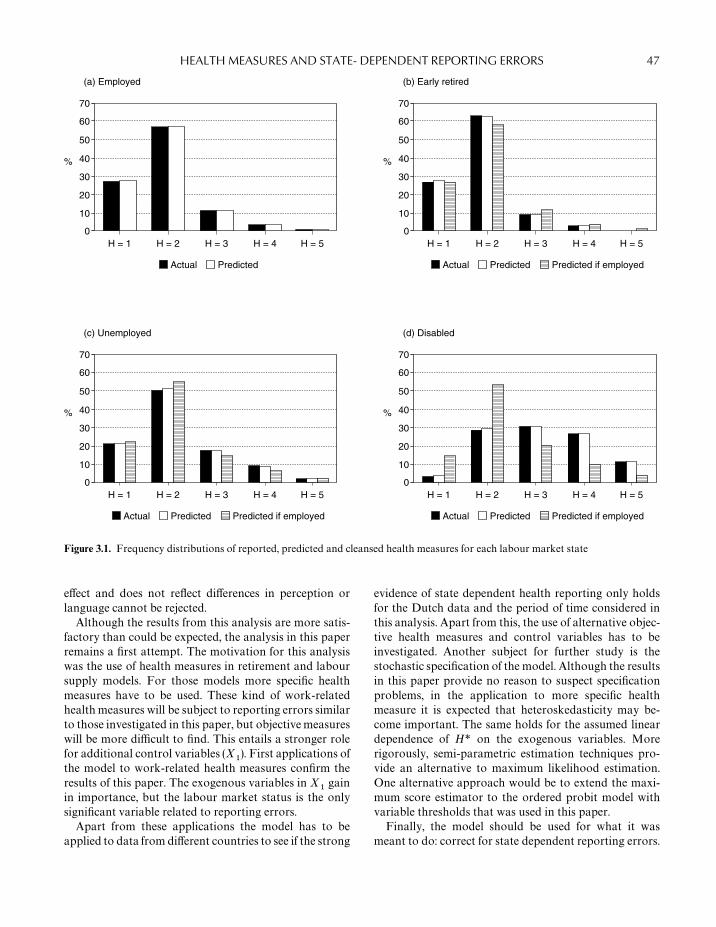
70

60

50

40

30

20

10

0H = 1

%

H = 2 H = 3

Actual

H = 4 H = 5

Predicted

(a) Employed

70

60

50

40

30

20

10

0H = 1

%

H = 2 H = 3

Actual

H = 4 H = 5

Predicted

(b) Early retired

70

60

50

40

30

20

10

0H = 1

%

H = 2 H = 3

Actual

H = 4 H = 5

Predicted

(c) Unemployed

70

60

50

40

30

20

10

0H = 1

%

H = 2 H = 3

Actual

H = 4 H = 5

Predicted

(d) Disabled

Predicted if employed

Predicted if employed Predicted if employed

Figure 3.1. Frequency distributions of reported, predicted and cleansed health measures for each labour market state

effect and does not reflect differences in perception orlanguage cannot be rejected.Although the results from this analysis are more satis-

factory than could be expected, the analysis in this paperremains a first attempt. The motivation for this analysiswas the use of health measures in retirement and laboursupply models. For those models more specific healthmeasures have to be used. These kind of work-relatedhealthmeasures will be subject to reporting errors similarto those investigated in this paper, but objectivemeasureswill be more difficult to find. This entails a stronger rolefor additional control variables (X

�). First applications of

the model to work-related health measures confirm theresults of this paper. The exogenous variables in X

�gain

in importance, but the labour market status is the onlysignificant variable related to reporting errors.Apart from these applications the model has to be

applied to data from different countries to see if the strong

evidence of state dependent health reporting only holdsfor the Dutch data and the period of time considered inthis analysis. Apart from this, the use of alternative objec-tive health measures and control variables has to beinvestigated. Another subject for further study is thestochastic specification of the model. Although the resultsin this paper provide no reason to suspect specificationproblems, in the application to more specific healthmeasure it is expected that heteroskedasticity may be-come important. The same holds for the assumed lineardependence of H* on the exogenous variables. Morerigorously, semi-parametric estimation techniques pro-vide an alternative to maximum likelihood estimation.One alternative approach would be to extend the maxi-mum score estimator to the ordered probit model withvariable thresholds that was used in this paper.Finally, the model should be used for what it was

meant to do: correct for state dependent reporting errors.


Table A3.1 Cross-tabulations of the health measures controlling for labour-market state

Employed Early retired

H� H�

H� 1 2 3 4 5 H� 1 2 3 4 5

1 225 305 21 2 1 1 82 132 7 2 02 167 335 47 9 3 2 57 123 15 4 03 116 305 71 29 4 3 31 124 19 4 14 25 97 48 10 3 4 9 26 11 1 05 6 37 13 9 0 5 3 12 2 2 06 6 32 17 12 3 6 1 6 5 1 07 0 8 11 4 5 7 0 2 2 2 1

Total 545 1119 228 75 19 Total 183 425 61 16 2

Unemployed Disabled

H� H�

H� 1 2 3 4 5 H� 1 2 3 4 5

1 44 49 4 2 0 1 7 30 8 4 12 25 70 14 4 0 2 5 27 28 14 43 25 68 28 5 4 3 4 60 63 32 84 8 50 15 11 1 4 4 28 39 36 115 2 12 7 3 1 5 0 12 18 13 66 2 9 9 11 1 6 1 27 35 43 157 1 4 12 10 3 7 1 8 16 36 28

Total 107 262 89 46 10 Total 22 192 207 178 73

One way would be to generate cleansed health measures.The application of those measures is not straightforwardas the imputation of cleansed measures will lead to errorsin variables biases. It would therefore be interesting toinvestigate whether the model of reporting behaviour canbe estimated simultaneously with a model of retirementor labour supply decisions.

ACKNOWLEDGEMENTS

We wish to thank Philip de Jong and the participants ofthe workshop on Health Econometrics in Antwerp, Sep-tember 1994, for their helpful suggests and comments.The authors are members of CERRA (Center for Econ-omic Research on Retirement and Aging) at Leiden Uni-versity. The research in this paper was financed by a grantfrom NESTOR (the Dutch Stimulation Program for Ag-ing Research) and from the Leiden University Speerpun-ten Program.

APPENDIX

Definition of variables

Age Age of the respondent (January 1993)Female Gender dummy, equals 1 if femaleEducation 1 Lower general

2 Lower vocational3 Medium general4 Medium vocational5 Higher general6 Higher vocational7 Academic

Married Dummy for marital status equals 1 ifmarried or living together

Religious Dummy, equals 1 if respondent attendsthe church at least once a week

H� Responses to question ‘How good wouldyou rate your health?’1 Very good2 Good3 Fair4 Sometimes good sometimes bad5 Bad


H� Hopkins symptom Checklist (HSCL)score1 Very good2 Good3 Above average4 Average5 Below average6 Bad7 Very bad

REFERENCES

1. Lambrinos, J. Health: A source of bias in labour supplymodels. Review of Economics and Statistics 1981; 63:206—212.

2. Parsons, D.O. Male labour force participation decision:health, reported health and economic incentives. Economica1982; 49: 81—91.

3. Anderson,K.H. andBurkhauser, R.V. The retirement-healthnexus: a new measure of an old puzzle. Journal of HumanResources 1985; 20: 315—330.

4. Bazzoli, G. The early retirement decision: New empiricalevidence on the influence of health. Journal of Human Re-sources 1985; 20: 214—234.

5. Butler, J.S., Burkhauser, R.V., Mitchell, J.M. and Pincus,T.P. Measurement error in self-reported health variables.Review of Economics and Statistics 1987; 69: 644—650.

6. Stern, S. Measuring the effect of disability on labour forceparticipation. Journal of Human Resources 1989; 24:361—395.

7. Bound, J. Self-reported versus objective measures of healthin retirement models. Journal of Human Resources 1991; 26:107—137.

8. Bartel, A. and Taubman, P. Health and labour market suc-cess: the role of various diseases. Review of Economics andStatistics 1979; 61: 1—8.

9. Lee, L.F. Health and wage: A simultaneous equation modelwithmultiple discrete indicators. International Economic Re-view 1982; 20: 199—221.

10. Chirikos, T.N. and Nestel, G. Further evidence on the econ-omic effects of poor health. Review of Economics and Statis-tics 1985; 67: 61—9.

11. Fuchs, V.R. Time preference and health: An exploratoryStudy. In: V.R. Fuchs (ed.), Economic Aspects of Health.Chicago: University of Chicago Press, 1982.

12. Sickless, R. and Taubman, T. An analysis of the health andretirement status of the elderly. Econometrica 1986; 14:1339—1356.

13. Burkhauser, R.V. The pension acceptance decision of olderworkers. Journal of Human Resources 1979; 14: 63—75.

14. Aarts, L.J.M. and de Jong, Ph.R. Economic Aspects of Dis-ability Behaviour. Amsterdam: North Holland, 1991.

15. Wagstaff,A. and vanDoorslaer, E.Measuring inequalities inhealth in the presence of multiple-category morbidity indi-cators.Health Economics 1994; 3: 281—291.

16. McKelvey, R. and Zavoina, W. A statistical model for theanalysis of ordinal level dependent variables. Journal ofMathematical Sociology 1975; 4: 103—120.


4

The Effect of Smoking on Health Using aSequential Self-selection Model

KAJAL LAHIRI AND JAE G. SONGDepartment of Economics, State University of New York at Albany,USA

INTRODUCTION

Ever since a causal relationship between cigarette smok-ing and coronary heart disease was reported at the MayoClinic in 1940, the effect of cigarette smoking on healthhas been extensively studied by both epidemiologists andsocial scientists. Now cigarette smoking is considered tobe the number one source of preventable morbidity andpremature mortality in the United States (see [1]). Sincethe 1960s, various public policy efforts have been devotedto reducing the prevalence of cigarette smoking. Still over25% of the population, or nearly 46.3 million adults in theUS and many more around the world smoke on a regularbasis [2].

There have been two approaches to reducing theprevalence of cigarette smoking: discouraging non-smokers from initiating, and encouraging smokers toquit. Even though smoking prevalence has steadily de-creased since the 1960s, this decrease has been due tomore people quitting but not due to fewer people initiat-ing [2]. Hence, a comprehensive model of smoking par-ticipation that considers both initiation and cessationbehaviour and their health effects is essential for develop-ing an effective public policy approach to reducing theprevalence of smoking, and in estimating the proper hu-man costs of cigarette smoking.

Unlike the consumption of a normal good, consump-tion of cigarettes increases not only the immediate satis-faction for smokers but also the probability of adversehealth effects in the future, neither of which are directlyobservable. Hence, the subjective judgement on the costsand benefits of cigarette smoking plays a crucial role insmoking participation decisions. This subjective judge-ment depends largely on the assessment of the probability

of the occurrence of side effects and the time preferencebetween the immediate benefits and the future side effectsof smoking.

An important factor affecting the initial smoking deci-sion is an individual’s prior belief on risks and benefitsfrom smoking, which could depend on his demographicand other socio-economic characteristics. Those who de-cide to smoke gather additional information throughtheir experience of smoking, and update their prior be-liefs. Based on the updated belief, a decision of continu-ation or cessation is made. Therefore, individual riskassessment of cigarette smoking takes a critical role ineach phase of the smoking cycle. Viscusi [3] studiedindividual risk perception and smoking decision by ques-tioning whether smokers are risk cognizants, and whetherthe risk perception is reflected in smokers’ behaviour.Viscusi [3] finds that the risk perception by the young isquite high, but it has no significant influence on theirinitiation behaviour.

Recently, the participation behaviours of smokers hasbeen empirically examined by Jones [4,5] and Hsieh et al.[6]. In these studies, the role of health condition, healthknowledge, social interaction, and other demographiccharacteristics are explored. There is another group ofstudies that examines the various human costs of smok-ing, such as health conditions, medical expenditures, andother economic consequences. Miller et al. [7] estimatesmedical care expenditures attributable to cigarette smok-ing. Mattson et al. [8] calculate the long-term risk ofdeath contributed by individual smoking status for vari-ous age groups. The later group of studies, however, treatsmoking status as exogenous, disregarding the dynamicinteraction between individuals’ health conditions andtheir smoking behaviour.

Econometric Analysis of Health Data. Edited by Andrew M. Jones and Owen O’Donnell© 2002 John Wiley & Sons Ltd. Previously published in Health Economics, Vol. 9; pp. 491—511 (2000). © John Wiley & Sons Ltd



In this paper, we study the participation behaviour ofsmokers, both initiation and cessation, and integratethem into a model of health consequences of smoking. Weexamine the possibility of the presence of any un-measured heterogeneity bias in the probability distribu-tions of smoking-related diseases for different smokinggroups, and we study whether the observed proportionsof smoking-related diseases in the sample correctly repre-sent the risk factor associated with a particular smokingbehaviour. The second issue we examine is whether theindividual smoking choices are made in a way that isconsistent with economic optimality. The rational addic-tion approach of cigarette smoking behaviour considerssmoking choice as the outcome of individual utility maxi-mization under uncertainty (see [9,10]). Even thoughthere are several empirical studies on the rational addic-tion model, they tend to focus on the role of price on thedemand for addictive goods without considering the roleof implicit health cost.

This paper is organized as follows. In ‘The Economet-ric Model’ and ‘Data and Empirical Specifications’, wedevelop a sequential selection model of smoking behav-iour based on a typical smoking cycle. ‘Empirical Strat-egy’ and ‘Empirical Estimates’ describe our data and theeconometric strategy and presents and discusses empiri-cal findings, respectively, and the paper ends with ‘Con-clusions’.

THE ECONOMETRIC MODEL

The smoking participation decisions, both initiation andcessation, are modelled as outcomes of utility maximiza-tion under uncertain occurrence of smoking-related dis-eases (SRDs) using a random utility model. Our model isbased on the following fundamental premise: the baseline(autonomous) and induced risk factors of cigarette smok-ing are not always equal for all individuals, and that eachindividual possesses a subjective prior belief concerningthe probability of occurrence of SRDs associated witheach smoking choice, and this belief is updated using theinformation gained through the smoking experience andthe realization of changes in his/her health condition.

Consider a simple two-period model with a time-separ-able indirect utility function. A rational individual livestwo periods indexed by t� 1, 2. At the beginning of eachperiod, individual i faces a decision to make a choicebetween two alternatives: to not smoke or to smoke,indexed by j� 0, 1 based on his own subjective judge-ment of the costs and the benefits of the alternatives. Thelength of each period varies across individuals. Let therebe two discrete states of health condition, good and bad,indexed by l� 1, 2. The bad-health state indicates the

presence of any undesirable health condition, caused byfactors including smoking.

Individual i possesses a prior belief on the probabilityof the occurrence of each health state for a given smokingstatus. This probability is optimally updated each period.Let P

��be the individual’s subjective probability for lth

health state when the smoking status is j. There are fourpossible states (S

��) of the world an individual could be

falling into. Further let U��

be an unobservable indirectutility of individual i choosing alternative j at period twhen his/her health condition is l. Then the expectedutility of each choice for each period t can be expressed asthe sum of the utilities in each health state weighted by itsprobability:

EU��

��

P��U�

��(4.1)

At the beginning of each period, an individual choosesalternative j over j� if and only if E

�U

��E

�U

��. The

discounted sum of expected utilities for the two periodsrealized at the beginning of period � is:

E�U��

��

��

��

P��U�

��(4.2)

where ��

is an individual-specific time preference par-ameter.

The initiation decision rule at the beginning of period 1is governed by the sign of I*

��E

�U

��E

�U

��. Once an

individual starts to smoke then another subsequent deci-sion rule can be defined in a similar way. The cessationdecision rule for the second period is governed by the signof I*

��E

�U

��E

�U

��. Thus, the selection criteria are:

Pr(choose to start smoking)� Pr(I*��

� 0)

Pr(choose not to start) � Pr(I*��

� 0)

Pr(choose to continue) � Pr(I*��

� 0, I*��

� 0)

Pr(choose to quit)� Pr(I*��

� 0, I*��

� 0)

I*��

and I*��

can be interpreted as present values of ‘net’utilities at the time of initiation and cessation. They arenot observable; we observe only their binary outcomes,I��

and I��

. There are three mutually exclusive outcomesof the selection process:

Group I (nonsmoker, I��

): I��

� 0

Group II (ex-smoker, I��

): I��

� 1 and I��

� 0

Group III (current smoker, I��

):

I��

� 1 and I��

� 1


The two selection equations are parameterized as:

I*��

�Z�� W

��

��

I*��

�Z�� W

��H

��

��(4.3)

where (Z��

,Z��

) are individual characteristics and(W

��, W

��) are the characteristics of the alternatives spe-

cific to the individual. The updated probability assess-ment at the beginning of the second period depends onthe realization of a change in health conditions (H

��)

which may or may not be related to the smoking status inperiod 1, individual characteristics (Z

�), and characteris-

tics of the alternatives specific to the individual (W��).

Finally, we specify an equation for the appropriateresponse variable for measuring the effect of the initiationand the cessation decisions. Since smoking participationdecisions heavily influence the probability of SRDs suchas lung diseases and various types of cancer, presence ofany SRDs is the most appropriate and direct outcomevariable for our purpose. Further, we will specify oneequation for each smoking group in order to capture thefull interactions among them (see [11]). The equationsare:

Y*��

�X��

��: nonsmokers’ disease equation

Y*��

�X��

��: ex-smokers’ disease equation

Y*��X

��

��: current smokers’ disease equation (4.4)

In Equations 4.3 and 4.4,Z��

and W��

areN�K�

andN�K

�vectors of explanatory variables; �

�and �

�are

K�� 1 and K

�� 1 vectors of unknown coefficients; Z

��,

W��

and H��

are N��K

, N

��K

�and N

��K

�vec-

tors of explanatory variables; and ��, �

�and �

�are

K� 1, K

�� 1 and K

�� 1 vectors of unknown coeffi-

cients; X��, X

��and X

��are N

��K

, N

�K

and

N��K

vectors of explanatory variables; �

�, �

�and �

�areK

� 1 vector of unknown coefficients; I*

��, I*

��, Y*

��, Y*

��and Y*

��are N� 1, N

�� 1, N

�� 1, N

� 1 and N

�� 1

unobservable latent indices; N�N�N

N

�and

N��N

N

�. We observe binary outcomes Y

��, Y

��, Y

��,

I�

and I�.

This completes our econometric model as a set ofswitching regressions with sequential self-selection rules.In the remainder of this paper, subscript i is omitted toavoid notational complexity. Also new variables C

�and

C�

will represent the independent variables in the firstand the second selection equations in Equation 4.3 withcoefficients �

�and �

�.

I*��C

��

�: initiation selection equation

I*��C

��

�: cessation selection equation

(observed, iff I�� 1)

Y*��X�

� �

�: nonsmoker’s disease equation

(observed, iff I�� 0)

Y*��X�

� �

�: ex-smoker’s disease equation

(observed, iff I�� 1, I

�� 0)

Y*��X�

� �

�: current smoker’s disease equation

(observed, iff I�� 1, I

�� 1)

The two sequential self-selection rules sort people intoobserved classes according to the expected present valueof indirect utility. Hence, the presence of SRDs actuallyobserved in each group are not random outcomes in thepopulation, but instead are self-censored nonrandomsamples. The initiation decision equation is defined overthe entire population, but the cessation decision equationis defined only over the subset of observations for thosewho have started to smoke.

DATA AND EMPIRICAL SPECIFICATIONS

We use data from Health and Retirement Study (HRS)Wave I which was released in May 1995. The HRS is anational longitudinal study on health, retirement, andeconomic status focusing on individuals both between1931 and 1941. A total of 12 652 individuals were inter-viewed during 1993, among these 2372 are single respon-dents and 5234 are paired (married or partnered) respon-dents. Their ages vary from 23 to 85 as of 1993. Mean agein the total sample is 55.6 and standard deviation is 5.66.Out of 12 652 individuals, 4626 are nonsmokers, 4588 areex-smokers, and 3438 are current smokers.

The main advantage of this data set for our purpose isthat the sample consists mainly of individuals in their 50s.The role of learning and regret throughout one’s smokingcycle and the effects of smoking on health can be morefully observed in this data set because most smokersinitiate smoking when they are relatively young. TheHRS also provides complete classification of individuals’smoking status as nonsmoker, ex-smoker, and currentsmoker. Further, HRS has extraordinary information oncurrent health conditions, health history, and varioussocio-economic factors. As a result, we are able to investi-gate the long-term health effects of 30—40 years of smok-ing.

To take full advantage of the data set for our purpose,we consider only individuals in the age group 52 andover.� We also drop those individuals who had quitsmoking after they were diagnosed with various types ofcancers and other smoking-related diseases to control forobvious endogeneity. As a result of these, our final sample

53THE EFFECT OF SMOKING ON HEALTH

for empirical analysis consists of 9109 individuals; amongthem 3287, 3368 and 2454 are nonsmokers, ex-smokers,and current smokers, respectively.�

The HRS data provides information that separatenever smokers from ever smokers, and ever smokers arefurther subdivided into ex-smokers and current smokers.Technically, nonsmokers in HRS are defined as thoseindividuals who smoked fewer than 100 cigarettes in his/her entire life time. Even though we observe completeoutcomes of the two participation decisions, estimation ofthese equations based on a single cross-sectional data setrequires careful thoughts. Fortunately, the data containlarge amounts of information on current as well as his-torical health, socio-economic, and demographic factors.Our variables are categorized as pure demographic, so-cial status, economic status, family life, current healthcondition and history, risk-taking behaviour, smokingrelated, and employment related variables. Some of thesevariables represent time invariant individual characteris-tics, such as sex, race, place of birth, and parents’ educa-tion. We also include some other variables which areassumed to capture individuals’ characteristics when theywere young such as religion, tidiness, smoking status ofthe spouse, and occupation. This inclusion is particularlyuseful for our empirical model specification because ourmodel contains two decisions that were possibly mademany years ago.

We select the explanatory variables for each equationbased on previous empirical specifications, theory, anddata availability. From an economics standpoint, theindividual’s risk belief is assumed to have an importantinfluence on the smoking behaviour. Barsky et al. [12]show that individual risk tolerance measured by HRSdata is positively related to risk-taking behaviour insmoking and drinking. Their estimated preference par-ameters are related to the behaviour of individuals, andtheir risk tolerance estimates make prediction of smokingbehaviour at least qualitatively correct. Viscusi [13,14]found some evidence that an individual’s smoking deci-sion responds to his/her risk perception. Differences insmoking behaviour among different demographic groupsare reported in various studies. The Surgeon Generals’report of 1985 noted differences in smoking behaviour,both initiation and cessation, between white-collar andblue-collar workers. Breslau and Peterson [15,16] re-ported that smoking cessation varies by sex, race, educa-tion, and number of cigarettes smoked daily. They alsofound that smoking and drinking habits are correlated.The prevalence of alcohol abuse or dependence was sig-nificantly higher in smokers than nonsmokers. For thethree SRD equations, we include occupation, smoking,nutrition, demographic, socio-economic, and generalhealth-related variables. To control further for individual

heterogeneity, we include variables related to occupation,occupational hazards, fundamental health condition in-dicators, socioeconomic status, life-styles, and insurancestatus.

Our key dependent variable is the presence of one ofthe SRDs, which include various lung diseases and typesof cancers that are directly related to smoking such ascancer of the abdomen, mouth, bladder, neck, nose, pan-creas, brain, bronchia, cervix, oesophagus, stomach,throat, tongue, kidney, liver, and lung. Selection of suchcancers is based on reports of the Surgeon General in1982, 1983, and 1984 on the health consequences of smok-ing and on various medical and public health literaturesuch as Bartecchi et al. [1], Mattson et al. [8], Yuan et al.[17] and Fielding [18]. Thus, our definition of SRD isvery broad, giving us a reasonable sample size of peoplehaving SRDs. Detailed definitions of variables are shownin Appendix A and descriptive statistics by smokingstatus for some key variables are summarized in Table4.1.

EMPIRICAL STRATEGY

Our empirical strategy is to estimate the model first by atwo-step probit method using the Heckman—Lee two-step method and to use the two-step estimates as startingvalues for full information maximum likelihood (FIML)estimation. The conditional expectations of the depend-ent variables using the properties of truncated normaldensity functions are:

E(I*�) �G

�

E(I*�� I

�� 1) �G

�E(�

��G

��

�)

�G�

��

�(G

�)

��(G

�)

E(Y*�� I

�� 0) �X

��E(�

��G

��

�)

�X��

��

��(G

�)

1 ��(G

�)

E(Y*�� I

�� 1, I

�� 0)

�X��E(�

�� G

��

�, �G

��

�)

�X��

��

�(G

�)�

�( �G*

�)

��(G

�, �G

�; �

��)

��

��(G

�)�

�(G*

�)

��(G

�, �G

�; �

��)

E(Y*�� I

�� 1, I

�� 1)

�X��E(�

�� G

��

�, �G

��

�)


Table 4.1 Descriptive statistics for selected variables

Whole sample Nonsmoker Ex-smoker Current smokerVariables mean mean mean mean

AGE 1.0000 0.9967 1.0088 0.9922ALCHOLIC 0.0543 0.0179 0.0537 0.1039ARTHRTS 0.3974 0.3836 0.4041 0.4067BADFIN 0.2244 0.1926 0.1900 0.3142BLOODPRS 0.4062 0.4061 0.4353 0.3663BMI 1.0000 1.0116 1.0189 0.9586CATHOLIC 0.2734 0.2616 0.2892 0.2673CHOLSTRL 0.2401 0.2443 0.2553 0.2135DIABTS 0.1123 0.1071 0.1232 0.1043DISEASE 0.0974 0.0542 0.0941 0.1597EVDRINK 0.6078 0.5196 0.6660 0.6459EXDRINK 0.2031 0.0904 0.2524 0.2865EXER 0.2098 0.2212 0.2432 0.1487FEDINS 0.1671 0.1263 0.1859 0.1960FINJOB 0.0520 0.0593 0.0454 0.0513FORNBORN 0.0973 0.1238 0.0900 0.0717GOODFAM 0.2211 0.2379 0.2396 0.1732HAZWORK 0.2040 0.1552 0.2224 0.2441HELTHINS 0.8572 0.8598 0.8893 0.8097INVEST 0.6253 0.6660 0.6758 0.5016IRA 0.4197 0.4551 0.4822 0.2865JOGAMILE 0.1447 0.1618 0.1571 0.1047LIFEINS 0.7098 0.6988 0.7527 0.6659MALE 0.5003 0.3614 0.6161 0.5273MARIDIST 0.5405 0.6109 0.5621 0.4165MARIED 0.7508 0.7682 0.7975 0.6634MILIT 0.2956 0.1935 0.3833 0.3121MYOPIC 0.1829 0.1682 0.1609 0.2327NETWORTH 1.0000 1.1744 1.0607 0.6834NEVERW 0.0349 0.0554 0.0187 0.0297PAREDU 0.2999 0.2823 0.3141 0.3040RACEB 0.1634 0.1667 0.1443 0.1850RACEW 0.7254 0.7037 0.7548 0.7143RELIGS 0.5256 0.6413 0.5220 0.3757RISKAVER 0.8717 0.8862 0.8735 0.8496SALESJOB 0.1547 0.1363 0.1485 0.1879SCHLYRS 1.0000 1.0202 1.0171 0.9494SERVJOB 0.0924 0.0931 0.0852 0.1015SPOSENSM 0.5117 0.5634 0.4840 0.4804SPOSEXSM 0.2855 0.2778 0.3480 0.1968TECHJOB 0.1277 0.1451 0.1455 0.0799WESTB 0.0784 0.0803 0.0808 0.0725

�X��

��

�(G

�)�

�(G*

�)

��(G

�,G

�;

��)

��

�(G

�)�

�(G

�)

��(G

�,G

�;

��)

where

G��C

��,

G��C

��,

G*��G

��

��G

�(1 ��

��)��

,

G*��G

��

��G

�(1 ��

��)��

.

��(·) and

�(·) are the standard g-variate normal distribu-

tion and density function, respectively.Thus, we can rewrite the equations with new error

terms which have zero conditional means:


I�

�G� �

�

I�

�G�

��

e�

Y��X

��

��

e�

Y��X

��

��

��

��

e�

Y��X

��

��

��

��

e�

(4.5)

where

��

��(G

�)

��(G

�),

��

��

�(G

�)

1 ��(G

�),

��

��(G

�)�

�( �G*

�)

��(G

�, �G

�; �

��),

��

��(G

�)�

�(G*

�)

��(G

�,G

�;

��),

��

��

�(G

�)�

�(G *

�)

��(G

�, �G

�; �

��)

and

��

��(G

�)�

�(G*

�)

��(G

�,G

�;

��).

Under the normality assumption, each of the aboveequations can be estimated sequentially by five separateprobit regressions with the appropriate Heckman—Leecorrections as specified in Equation 4.5. Note that theerror terms e

�, e

�, e

�and e

�are heteroskedastic by con-

struction, and if there are overlapping variables in theselection and disease equations, the problem of significantmulticollinearity may result in the structural equations.

ENDOGENEITY OF SOME HEALTH VARIABLE

A recent debate between Jones [4,5], and Shmueli [19]deals with the issue of endogeneity of health variables inthe cessation decision equation. The health variables in-cluded in our equations are based more objectively onphysical activity limitations and health history, which areexpected to develop independent of smoking.

Blundell and Smith [20] provide a simple way to testfor endogeneity by a two-stage approach. The first stageis to regress the suspicious variables on exogenous vari-ables. The second step is to estimate the original probitequation with the residuals from stage 1 as additionalregressors and to jointly test the hypothesis that coeffi-

cients of the residuals are zeros. Since our suspicioushealth variables are binary, we generated probit general-ized residuals (see [21,22]). The probit generalized resid-uals for a model Y*

��X

��

�are given by:

�� Y��

�(X

��R�)

�(X

��R�)

� ((1 ��(X

��R�))��

�(X

��R�)�� (4.6)

We tested the endogeneity of EXER (exercises regularly),JOGAMILE (can jog a mile with no difficulty),BLOODPRS (blood pressure), CHOLSTRL (choles-terol), ARTHRTS (arthritis), and DIABTS (diabetes) inthe cessation decision and BLOODPRS, CHOLSTRL,ARTHRTS, and DIABTS in the switching disease equa-tions.� The �� statistics for the null hypotheses that theseadditional coefficients are zero for cessation, non-smokers’, ex-smokers’ and current smokers’ equations areobtained as 6.585 (df� 6), 3.474 (df � 4), 3.232 (df � 4)and 3.123 (df � 4), respectively. These are not statisticallysignificant at the 5% level of significance. Our specifica-tions originally included a few other health variables, butwe dropped them because they did not pass the en-dogeneity test.� These variables were replaced by theinstruments used to test for their endogeneity, wheneverthey were statistically significant. Thus, we interpret ourdisease equations as purely reduced form specifications.

HETEROSKEDASTICITY

We examine the presence of heteroskedasticity using thefollowing formulation [23]:

Var(��) ��

�� [exp(V

� )]�

Y*��X

��

�(4.7)

where V�

is 1 � p vector of observations on a subset ofvariables, and � is a vector of corresponding parameters.Then log of likelihood function is:

ln l ��

Y�ln �

��X

��

exp(V� )�

(1 � Y�) ln�1 ��

��X

��

exp(V� )�� (4.8)

Once this likelihood function is maximized, we caneasily check for heteroskedasticity by the likelihood ratiotest because � 0 implies homoskedasticity. Further, wecan identify the special structure of heteroskedasticityand are able to correct it by feasible GLS [24]. The resultsindicated that significant heteroskedasticity exists in all


our equations at the 5% level. As a result, we specified ourequations after allowing for heteroskedasticity:

I*�

�D� �

�I*�

�D�

��*��

��

Y*��D

�

��*��

e�

Y*��D

�

��*��

��

�*��

e�

Y*��D

�

��*��

��

�*��

e�

(4.9)

where

D��

(C��)

exp(V� �),

D��

(C��)

exp(V� �),

D��

X��

exp(V� �),

D��

(X��)

exp(V� �),

D��

(X��)

exp(V� �)

and Vs are the variables which condition heteroskedastic-ity for each equation. �*s are defined in the same way asin Equation (5) with Gs replaced by Ds.

NORMALITY TESTS

Pagan and Vella [25] derived a normality test for thetobit model with selectivity that can be directly applied toour probit model with selectivity. Since our cessation andnonsmokers’ disease equations involve a single selection,we can apply the test developed by Pagan and Vella withminor modifications. However, we want to estimate ourstructural model by FIML, which requires evaluation oftrivariate CDFs. As a result, we use the normality testbased on Edgeworth expansion of CDF suggested by Lee[26], generalized to the trivariate case by Lahiri and Song[27]. Here we test for the bivariate normality of (�

�, �

�)

and the trivariate normality of (��, �

�, �

�) and (�

�, �

�, �

�).

The �� statistics were calculated as 12.97 (df � 9), 27.42(df� 25), 31.64 (df � 25), respectively. Since these valuesare less than the critical �� values at the 5% level ofsignificance, we did not reject the multivariate normalityassumption in our context. We should point out thatwithout the heteroskedasticity correction, the normalityassumption would have been resoundingly rejected in oursample (see [27]).

FULL INFORMATION MAXIMUM LIKELIHOODESTIMATION

The inefficiency of the two-step method relative to maxi-mum likelihood has been critically examined by Nelson[28], who suggested the more difficult MLE. The poorperformance of Heckman—Lee two-step method is alsoreported in Nawata and Nagase [29] and Stolzenbergand Relles [30]. Their results, based on Monte Carlo andempirical examples, suggest that the two-step methodmay not be a dependable estimator when there is strongmulticollinearity between independent variables (X) andselectivity correction terms (�s). If there are no overlap-ping variables in the selection and the outcome regressionequations, then the multicollinearity may not be veryhigh. Since we have overlapping variables, especially inthe second selection equation, we can not rule out thepossibility of significant multicollinearity. As a result, it isadvisable to estimate the model by FIML for correctinferences (see [31] for further discussion).

The log of likelihood function for the model Equation4.9 is:

ln L(��,

�, �

�,

�,�

�, �

�,

�, �

�,

�,

��

, ��

, ��

, ��

, ��

, ��

)

��

�(1 � I�)Y ln �

�( �D

�,D

�; �

��)

(1 � I�)(1 � Y) ln �

�( �D

�, �D

�;

��)

I�(1 � I

�)Y ln �

(D

�,�D

�,D

�;

��

, ��

, ��

) I�(1 � I

�)(1 � Y)

� ln �(D

�, �D

�, �D

�; �

��,

��, �

��)

I�I�Y ln �

(D

�,D

�,D

�;

��,

��,

��)

I�I�(1 � Y) ln �

(D

�,D

�,�D

�;

��, �

��, �

��)

(4.10)

where ��(. , . , ; .) and �

(. , . , . , ; . , . , .) are the standard bi-

variate and trivariate densities, respectively. The par-ameters are �

�, �

�, �

, �

�, �

�, �

�, and 5 � 5 covariance

matrix of disturbances, :

��1

��

��

��

��

1 ��

��

��

��

��

1 ��

��

��

��

��

1 ��

��

��

��

��

1 �Note that

��,

��,

��and

��do not explicitly appear in

the likelihood function. It is well known that ��

, ��

and


��

are not identified because the likelihood function doesnot depend on these parameters (for further discussion onthis issue see [32]). Another parameter,

��, is also not

identified because the second selection equation is irrel-evant for the nonsmoker group, and, hence, it is not in thelikelihood function. This is because our two selectionequations classify the sample not into four categories butinto three categories. Hence, an additional restriction(

�� 0) on the variance covariance matrix is required

for identification. The rest of the parameters — (K�

K�) 6 (K

K

�K

�) 7 3K

elements of re-

gression coefficients ��, w

�, �

�, w

�, �

�, �

�,

�, �

�and

�,

plus six elements of the covariance matrix ��

, ��

, ��

,��

, ��

and ��— are identifiable. It is well known that

the likelihood function of the multivariate probit model isnot globally concave, unlike that of the univariate probitmodel. The complexity of the likelihood function makesthe FIML estimation difficult, and there is no ready-madeguarantee that one has reached the global maximum.

We estimate the model by FIML with starting valuesfrom the Heckman—Lee two-step method with pre-testedforms of heteroskedasticity using GAUSS (version 3.2.4).FIML has seldom been used to estimate switching re-gression models with double selection because of com-putational difficulty. One useful tip to save a significantamount of computing time is to arrange the data by eachof the six non-overlapping groups and maximize a form ofthe log of likelihood function given in Equation 4.11rather than Equation 4.10:

ln L(��,

�, �

�,

�, �

�, �

�,

�, �

�,

�,

��

,��

, ��

, ��

, ��

,��

)

� ��

ln ��( �D

�,D

�;�

��)

��

ln ��( �D

�, �D

�;

��)

��

ln �(D

�, �D

�,D

�;�

��,

� ��

, ��

) ��

� ln �(D

�, �D

�, �D

�; �

��,

��, �

��)

��

ln �(D

�,D

�,D

�;

��,

��,

��)

��

ln �(D

�,D

�, �D

�;

��

, ��

, ��

) (4.11)

If one wishes to maximize the likelihood function as

written in Equation 4.11, GAUSS will evaluate two bi-variate normal CDFs and four trivariate normal CDFsfor each observation. In our estimation, we have savedmore than three quarters of the computing time by maxi-mizing (4.7). We also found that a ‘good’ starting value iscritical to achieving smooth convergence. Further, wenormalized all continuous variables by their means toprevent any possible interruption during the maximiza-tion of the likelihood function. We use the Berndt—Hall—Hall—Hausman (BHHH) algorithm for the FIMLestimation and it took 29 iterations (with running timeapproximately 673 minutes in a 400 Hertz (Htz) PC) toconverge with a pre-set tolerance level of 0.00001.� Thevariance—covariance matrix of the estimated structuralparameters is obtained from the final information matrixon convergence. Interestingly, the estimates from the two-stage method and the FIML were very close except forthe selectivity correction terms.�

EMPIRICAL ESTIMATES

SELECTION EQUATIONS

Table 4.2 presents heteroskedasticity corrected two-stepand FIML estimates of the first selection equation to-gether with marginal effects and odd ratios associatedwith different explanatory variables. To check for good-ness-of-fit we compute various measures of pseudo R�.Among those McKelvey and Zavonia’sR� is 0.23, and thecorrect prediction rate is about 70%.

The initiation decision varies by different demographiccharacteristics; males tends to initiate more often thanfemales. Participation in regular religious services (RE-LIGS), having a stable marriage life (MARIDIST), andhaving a nonsmoking spouse (SPOUSNSM) have highnegative correlation with initiation. Individual drinkingbehaviour (EVDRINK, EXDRINK) has a significantpositive effect. We also find that the propensity to initiatevaries across different ethnic groups and education levels.SCHLYRS (school years) has a significant nonlinear ef-fect on the initiation decision.

The variables RISKAVER, MYOPIC, and INVESTrepresent individuals’ attitudes toward risk and play amajor role in initiation. The variable RISKAVER repre-sents individual risk aversion and MYOPIC representsan aspect of individual’s time preference. For example, theindividual with MYOPIC� 1 may be considered as ashort-sighted individual who tends to prefer the immedi-ate benefits of smoking over the future costs of healthdeterioration. These risk variables, which we can take tobe largely time-invariant, turned out to have substantiveimpact on the initiation decision; odd ratios and marginal


Table 4.2 Estimates for the initiation equation

SE Odds MarginalVariable Two-step FIML (FIML) ratio effect

Constant 0.8821 0.8964 0.1599 2.4508 0.3091MALE 0.4142 0.4173 0.0451 1.5179 0.1452RACEW 0.0871 0.0835 0.0559 1.0871 0.0305RACEB 0.1053 0.1101 0.0754 1.1164 0.0369FORNBORN �0.2378 �0.2483 0.0591 0.7801 �0.0833WESTB �0.1118 �0.1104 0.0554 0.8955 �0.0392SOUTHB 0.0189 0.0145 0.0339 1.1046 0.0066SCHLYRS 0.5224 0.5205 0.2507 1.6829 0.1831SCHLYRS2 �0.5048 �0.5071 0.1397 0.6022 �0.1769PAREDU 0.0740 0.0784 0.0308 1.0816 0.0259CATHOLIC 0.1495 0.1520 0.0362 1.1642 0.0524RELGIS �0.2729 �0.2764 0.0341 0.7585 �0.0956MILIT 0.1477 0.1487 0.0424 1.1603 0.0518MARIDIST �0.3707 �0.3710 0.0354 0.6900 �0.1299EVDRINK 0.2950 0.2996 0.0423 1.3493 0.1034EXDRINK 0.8802 0.8823 0.1904 2.4165 0.3085SPOUSNSM �0.3499 �0.3488 0.0343 0.7055 �0.1226NETWORTH �0.0155 �0.0156 0.0057 0.9845 �0.0054INVEST �0.1482 �0.1489 0.0354 0.8617 �0.0519SALESJOB 0.1236 0.1270 0.0397 0.1354 0.0433FINJOB �0.0698 �0.0691 0.0607 0.9332 �0.0245TECHJOB 0.0787 0.0798 0.0477 1.0831 0.0276SERVJOB 0.0408 0.0401 0.0469 1.0409 0.0143NVRWORKD �0.2655 �0.2677 0.0778 0.7651 �0.0931RISKAVER �0.0817 �0.0826 0.0428 0.9207 �0.0286MYOPIC 0.0650 0.0678 0.0384 1.0702 0.0228CLEAN �0.0763 �0.0773 0.0292 0.9256 �0.0267BMI �0.3763 �0.3834 0.0820 0.6815 �0.1319

RACEB 0.3005 0.3088 0.0826MARIDIST �0.2341 �0.2302 0.0602EVDRINK 0.1838 0.1862 0.0586 HeteroskedasticityEXDRINK 0.3354 0.3348 0.1334 SpecificationSPOUSNSM �0.1738 �0.1677 0.0561

effects of RISKAVER, MYOPIC, and INVEST are (0.92,1.07. 0.86) and (�0.029, 0.022, �0.05), respectively. Thisevidence indicates that risk-average individuals tend notto initiate and that individuals with higher time prefer-ences for the immediate tend to initiate more often. Othersocio-economic status variables have significant explana-tory power to explain individuals’ initiation decisions.The direction of contributions from these variables areconsistent with previous studies.

Table 4.3 presents estimates from heteroskedasticity-corrected two-step estimator of the second selectionequation (continuation decision) by FGLS and FIMLprocedures together with the marginal effects and oddratios. McKelvey—Zavonia’s R� is 0.31 and the correctprediction rate is again about 70%. In terms of the R�

measure, the fit of the second selection equation is slightlybetter than that of the first selection equation. As onewould expect, spouse’s cessation decision (SPOSEXSM)

has very strong effect on individual’s cessation decision.Spouse’s health status and the number of children in thehousehold were not significant.

An interesting finding is that the presence of currentgood health conditions (EXER, JOGAMILE) and alsobad health conditions (BLOODPRS, CHOLSTRL, DIA-BTS) have strong positive effects on the propensity forcessation. When people realize that they have developedsome bad health conditions which might be aggravatedby smoking, they tend to quit (see [4,19]). Currentsmokers who still enjoy good health sometimes quit inorder to maintain the good health. This evidence simplyimplies that there are two groups of ex-smokers in oursample — one group quits in order to restore better health(curative), and the other group quite in order to maintaingood health (preventive).

Risk variables in the cessation decision equation alsohave very interesting implications. RISKAVER, MY-


Table 4.3 Estimates for the continuation equation


Constant 0.9862 1.0069 0.2036 2.7371 0.3900MALE �0.1056 �0.1202 0.0346 0.8867 �0.0417RACEB 0.1491 0.1619 0.0701 1.1757 0.0590RACEW 0.0917 0.1343 0.0662 1.1437 0.0363FORNBORN �0.1211 �0.1094 0.0534 0.8964 �0.0479CATHOLIC 0.0556 0.0489 0.0264 1.0501 0.0220RELIGS �0.1972 �0.1968 0.0351 0.8214 �0.0779MARRIED �0.1635 �0.1633 0.0451 0.8493 �0.0646NOMARAGS 0.0450 0.0443 0.0197 1.0453 0.0178HOUSE �0.0533 �0.0497 0.0250 0.9515 �0.0211EXER �0.1408 �0.1485 0.0341 0.8620 �0.0557ALCHOLIC 0.1896 0.1858 0.0495 1.2042 0.0749CLEAN �0.1100 �0.1156 0.0267 0.8908 �0.0435BADFIN 0.0799 0.0814 0.0287 1.0848 0.0316SPOUSNSM �0.2940 �0.2873 0.0574 0.7428 �0.1163SPOUSXSM �0.4094 �0.4209 0.0600 0.6565 �0.1619OWNRV �0.1512 �0.1566 0.0654 0.8550 �0.0598IRA �0.1353 �0.1465 0.0309 0.8637 �0.0535LIFEINS �0.0373 �0.0408 0.0260 0.9600 �0.0148RISKAVER �0.0498 �0.0486 0.0319 0.9526 �0.0197HELTHINS �0.0872 �0.0827 0.0339 0.9206 �0.0345SCHLYRS 0.5217 0.5413 0.2149 1.7182 0.2063SCHLYRS2 �0.3956 �0.4102 0.1186 0.6635 �0.1564JOGAMILE �0.1466 0.1696 0.0417 1.1848 �0.0580BLOODPRS �0.0946 �0.0983 0.0266 0.9064 �0.0374CHOLSTRL �0.0421 �0.0443 0.0254 0.9567 �0.0166DIABTS �0.0356 �0.0383 0.0355 0.9522 �0.0141ARTHRTS �0.0260 �0.0280 0.0226 0.9724 �0.0103SALESJOB 0.0745 0.0725 0.0294 1.0752 0.0295FINJOB 0.0946 0.0978 0.0492 1.1027 0.0374MYOPIC 0.0691 0.0700 0.0296 1.0725 0.0273ADDICTION 0.0595 0.0593 0.0142 1.0611 0.0235BMI �0.7590 �0.8134 0.1165 0.4433 �0.3001R12 0.1137 0.1590 0.1227

MALE 0.1671 0.1516 0.0671RACEW �0.5697 �0.5365 0.0904MARRIED �0.1372 �0.1209 0.0951 HeteroskedasticitySPOUSNEM �0.2414 �0.2112 0.0832 SpecificationOWNRV 0.2249 0.1994 0.1233

OPIC, IRA, LIFEINS, and HELTHINS are the variablesthat can capture individual risk behaviour. Our resultsshow that those individuals who have higher time prefer-ences for the current time continue to smoke. The vari-ables LIFEINS and HELTHINS represent individuals’attitudes towards health risk, and these variables alsohave a meaningful interpretation. Individuals who haveindividual retirement accounts (IRA) can be consideredto be more financially well planned, and the variable IRAhas a positive contribution to the cessation decision.Schooling (SCHLYRS, SCHLYRS2) and Body Mass In-dex (BMI) variables have significant non-linear effects onthe cessation decision. Another interesting variable is the

cigarette addiction variable (ADDICTION) which is de-signed to capture the approximate strength of smokers’cigarette addictions. As one would expect, our result indi-cates that the stronger the addiction, the harder it is toquit. Also a stable married life (MARRIED, NO-MARAGS) and drinking habit (ALCOHOLIC) have sig-nificant effects on the cessation decision. We also observevariations in cessation propensity by different demo-graphic, occupational, and economic classes, and they areconsistent with prior findings.


Table 4.4 Estimates for the nonsmoker’s disease equation


Constant �2.7242 �2.6669 0.9493 0.0695 �0.3230MALE �0.0873 �0.0747 0.1033 0.9280 �0.0104RACEB 0.2413 0.2329 0.1699 1.2623 0.0286FORNBORN 0.4258 0.4149 0.1692 1.5142 0.0505WESTB 0.6618 0.6488 0.2103 1.9132 0.0785MARIDIST �0.0532 �0.0605 0.0898 0.9413 �0.0063BLOODPRS 0.4400 0.4388 0.1589 1.5508 0.0522CHOLSTRL 0.1947 0.1931 0.0760 1.2130 0.0231DIABTS �1.0859 �0.0799 0.5215 0.3396 �0.1287ARTHRTS 0.2126 0.2132 0.0787 1.2376 0.0252EXDRINK �0.1684 �0.1548 0.1285 0.8566 �0.0200BADFIN 0.2037 0.2042 0.0832 1.2265 0.0242GOODFAM 0.0344 0.0324 0.1030 1.0329 0.0041HAZWORK 0.3111 0.3122 0.0871 1.3664 0.0369AGRIJOB 0.1120 0.1108 0.1879 1.1172 0.0133SALESMAN �0.0824 �0.0806 0.1495 0.9226 �0.0098SERVJOB �0.0907 �0.0885 0.1188 0.9153 �0.0108NVRWORKD 0.5355 0.5319 0.1786 1.7022 0.0635FEDINS 0.2415 0.2406 0.0933 1.2720 0.0286LIFEINS 0.0312 0.0306 0.0808 1.0311 0.0037RISKAVER �0.0051 �0.0081 0.1106 0.9919 �0.0006MYOPIC �0.2119 �0.2067 0.1512 0.8133 �0.0251SPOUSNSM 0.1722 0.1634 0.1291 1.1775 0.0204SPOUSXSM 0.1780 0.1773 0.1281 1.1940 0.0211NOJOBS �0.0264 �0.0256 0.0641 0.9747 �0.0031NOMARAGS 0.1876 0.1884 0.0863 1.2073 0.0222AGE 0.3834 0.3763 0.4647 1.4569 0.0455SCHOLYRS �0.0697 �0.0741 0.1334 0.9286 �0.0083NETWORTH �0.0426 �0.0433 0.0344 0.9576 �0.0051BMI 0.1914 0.1863 1.2774 1.2048 0.0227BMI2 0.0138 0.0144 0.5548 1.0145 0.0016Rln �0.0247 0.0130 0.1791

RACEB �0.3961 �0.3923 0.1701FORNBORN �0.5785 �0.5774 0.1665WESTB �0.6623 �0.6529 0.2747BLOODPRS �0.3126 �0.3127 0.1420 HeteroskedasticityDIABTS 0.9055 0.9067 0.2777 SpecificationNVRWORKD �0.7137 �0.7206 0.2851MYOPIC 0.4190 0.4189 0.1356

SWITCHING DISEASE EQUATIONS

Tables 4.4—4.6 present estimates of the disease equationsby two-step and FIML methods for the three smokingstatus groups. We specify our switching disease equationsusing a number of demographic, occupational, economic,and fundamental health condition variables. An interest-ing variable is HAZWORK, which represents occupa-tional exposure to hazards. In some sense, HAZWORKalso represents individual risk-taking behaviour as well.The occupational exposure to hazards has significanteffect on the probability of the occurrence of the SRDs forall three smoking groups. There are direct and indirect

effects of this variable. The direct effect in the contribu-tion from the exposure. Some workers work in hazardousoccupations not because they prefer them, but becausethey have no other choices. The indirect effect comesbecause individuals who work in hazardous occupationsare often risk-takers (see [33]), and such attitudes canhave positive effects on the probability of SRDs. A part ofthe indirect effect is expected to manifest itself through theselectivity correction terms.

The variable FEDINS, which indicates health insur-ance coverage by federal health insurance programs suchas Medicaid and VA, has a positive effect on the probabil-ity of having SRDs for all three smoking groups. The


Table 4.5 Estimates for the ex-smoker’s disease equation


Constant �0.8954 �1.1841 0.8318 0.3060 �0.1379MALE �0.1548 �0.1390 0.0948 0.8702 �0.0238RACEB �0.1923 �0.1884 0.1025 0.8283 �0.0296FORNBORN �0.5729 �0.5346 0.2005 0.5859 �0.0882WESTB �0.0830 �0.0777 0.1117 0.9252 �0.0128MARIDIST 0.0794 0.0886 0.0911 1.0926 0.0122BLOODPRS �0.2342 �0.3002 0.1871 0.7407 �0.0361CHOLSTRL 0.0018 0.0083 0.0692 1.0083 0.0003DIABTS 0.1398 0.1355 0.0886 1.1451 0.0215ARTHRTS 0.1581 0.1585 0.0647 1.1718 0.0244EXDRINK 0.1066 0.0986 0.0784 1.1036 0.0164BADFIN 0.0811 0.0602 0.0777 1.0620 0.0125GOODFAM 0.2763 0.3265 0.1623 1.3861 0.0425HAZWORK 0.4941 0.5138 0.1582 1.6716 0.0761AGRIJOB �0.0056 �0.0026 0.1825 0.9974 �0.0009SALESMAN �0.9838 �0.3988 1.3063 0.2469 �0.1515SERVJOB �0.0651 �0.0654 0.0962 0.9367 �0.0100NVRWORKD �0.2946 �0.2985 0.2684 0.7419 �0.0454FEDINS 0.2136 0.2146 0.0838 1.2394 0.0329LIFEINS �0.0581 �0.0461 0.0698 0.9549 �0.0090RISKAVER �0.1243 �0.1189 0.0910 0.8879 �0.0191MYOPIC 0.2735 0.3380 0.1666 1.4021 0.0421SPOUSNSM 0.0467 0.0650 0.1030 1.0672 0.0072SPOUSXSM 0.1109 0.1459 0.1039 1.1571 0.0171NOJOBS �0.0631 �0.0683 0.0455 0.9340 �0.0097NOMARAGS 0.1436 0.1392 0.0681 1.1494 0.0221AGE 0.3400 0.3822 0.4096 1.4655 0.0524SCHOLYRS �0.3158 �0.2746 0.1272 0.7599 �0.0486NETWORTH �0.0209 �0.0196 0.0217 0.9806 �0.0032BMI �1.8797 �1.6930 1.2346 0.1840 �0.2895BMI2 0.8676 0.8014 0.5460 2.2287 0.1336CIGARETS 0.2299 0.2219 0.0448 1.2484 0.0354R1x 0.2359 0.2230 0.2485R2x �0.2189 �0.3908 0.1743

BLOODPRS 0.2710 0.2659 0.1206GOODFAM �0.4824 �0.4197 0.1386HAZWORK �0.3551 �0.2886 0.1475 HeteroskedasticitySALESMAN 0.6186 0.6660 0.4368 SpecificationMYOPIC �0.3588 �0.3315 0.1439

marginal effect of FEDINS for nonsmokers, ex-smokers,and current smokers are 0.03, 0.03, and 0.08, respectively,implying that the interaction of smoking status and FED-INS is a significant factor in the health production func-tion (see [11]). Since FEDINS captures mostly peoplewith low socio-economic status, these estimates suggestthat smoking by individuals has a considerable social costas well. Unstable married life (NOMARAGS) also has asignificant impact on the presence of the diseases for allthree groups of smokers. We also find demographic vari-ations in the incidence of SRDs.

One of the most significant findings of this study is thepresence of significant selectivity coefficients in previous

smokers’ and current smokers’ disease equations. Some ofthe selectivity coefficients in FIML estimation turned outto be substantially different from those in two-step esti-mations — underscoring the importance of FIML ap-proach in these kinds of models. The selectivity coefficientin the nonsmokers’ equation turned out to be insignifi-cant. The statistically significant selectivity coefficients inthe last two disease equations imply the endogenous na-ture of switching in our structural model. We shouldemphasize that we took utmost care to fully specify ourfive equations such that the significance of the selectivityterms is not due to the omission of observable explana-tory variables. For instance, interaction of a number of


Table 4.6 Estimates for current smoker’s disease equation


Constant �0.9730 �0.8839 0.8575 0.4132 �0.1590MALE 0.0275 �0.0065 0.1638 0.9935 0.0045RACEB �0.5621 �0.5266 0.1262 0.5906 �0.0919FORNBORN �0.6234 �0.6189 0.1976 0.5385 �0.1019WESTB �0.2598 �0.2481 0.1523 0.7803 �0.0425MARIDIST 0.0584 0.0569 0.0976 1.0585 0.0095BLOODPRS 0.1616 0.1477 0.0811 1.1592 0.0264CHOLSTRL 0.1864 0.1697 0.0915 1.1849 0.0305DIABTS �0.1212 �0.0644 0.2057 0.9376 �0.0198ARTHRTS 0.3358 0.3250 0.0798 1.3840 0.0549EXDRINK 0.0223 0.0043 0.1047 1.0043 0.0036BADFIN 0.2615 0.2610 0.0951 1.2982 0.0427GOODFAM �0.2212 �0.2172 0.1306 0.8048 �0.0361HAZWORK 0.2300 0.2224 0.0935 1.2491 0.0376AGRIJOB 0.5055 0.4835 0.2286 1.6217 0.0826SALESMAN �0.3303 �0.3215 0.1484 0.7251 �0.0540SERVJOB �0.1556 �0.1485 0.1196 0.8620 �0.0254NVRWORKD 0.5811 0.5481 0.1791 1.7300 0.0950FEDINS 0.4773 0.4648 0.1025 1.5917 0.0780LIFEINS �0.2028 �0.1435 0.1442 0.8663 �0.0331RISKAVER �0.0055 �0.0086 0.1035 0.9914 �0.0009MYOPIC 0.0855 0.0894 0.0869 1.0935 0.0140SPOUSNSM 0.1659 0.1583 0.1065 1.1715 0.0271SPOUSXSM 0.2418 0.2105 0.1355 1.2343 0.0395NOJOB 0.0061 0.0026 0.0586 1.0026 0.0010NOMARAGS 0.1321 0.1352 0.0590 1.1448 0.0216AGE 1.0138 0.9496 0.5889 2.5847 0.1657SCHOLYRS �0.2571 �0.2513 0.1692 0.7778 �0.0420NETWORTH �0.0249 �0.0237 0.0414 0.9766 �0.0041BMI �2.2286 �2.2623 1.0911 0.1041 �0.3642BMI2 0.6494 0.6637 0.5072 1.9420 0.1061CIGARETS 0.1854 0.1875 0.0682 1.2062 0.0303R1c 0.1777 0.0931 0.3218R2c �0.3443 �0.2373 0.1452

MALE �0.1564 �0.1497 0.1336DIABTS 0.3646 0.3744 0.2216 HeteroskedasticityNVRWORKD �0.8484 �0.9518 0.3737 SpecificationLIFEINS 0.3288 0.3080 0.1316

statistically significant explanatory variables were notfound to be important in the specifications.

FURTHER IMPLICATIONS OF OUR FINDINGS

The model estimated in this paper provides a way toidentify the true risk of smoking by correcting the self-selection problem in the observed proportions of SRDs indifferent smoking groups. The evidence on the presence ofunobserved heterogeneity in ex-smokers’ and currentsmokers’ disease equations suggests that the risk factorfor smokers may be different from that of nonsmokers,

even if smokers had never smoked. The coefficients(

��,

��) from the initiation equation are both positive,

but they are not significant at the 5% level. On the otherhand, the coefficients (

��,

��) from the cessation equa-

tion are both negative and statistically significant at the5% level. The significance of these terms suggests that theobserved relative frequencies of SRDs in the sample arebiased estimates of the true risk factors for the ex-smokersand the current smokers. The observed proportionsbased on our sample indicate that the probability ofgetting SRDs for ex-smokers and current smokers are9.41% and 15.97%, respectively. The signs of the coeffi-cients (

��,

��) indicate the direction of the selection bias.


Table 4.7 Counter-factual risk factor predictions

Counter-factual smoking status

Observed smoking E[Y�� .] E[Y

� .] E[Y

�� .]

status (None) (Ex.) (Current)

None (I�� 0) 0.054 0.056 0.111

Ex (I�� 1, I

�� 0) * 0.094 0.214

Current (I�� 1, I

�� 1) * 0.082 0.159

The observed risk factors have two components: riskfactor due to smoking and selectivity. The estimatednegative values of

��and

��capture an unobservable

negative correlation between the propensity of gettingSRDs and the propensity of continuing to smoke. Ignor-ing this correlation, which manifests through the cessa-tion selection, would yield an upward bias for ex-smokers’ and downward bias for current smokers’ riskfactors. Since the signs of the selectivity coefficients allowus to make other interesting inferences, we devote the restof this section to interpreting the results.

Our prediction shows that the true mean risk factor forex-smokers is about 6%, which is slightly more than thatfor nonsmokers and much less than the observed riskfactor (9.41%). The risk factor for current smokers isabout 20%, which is much higher than the observed riskfactor for current smokers (15.9%). This finding hassignificant implications for previous empirical studies onthe costs of cigarette smoking. For example, Miller et al.[7] estimated medical care expenditures attributed tocigarette smoking based on observed frequencies ofSRDs, without considering the unobserved heterogeneityin the baseline risk factors of smokers. In order to esti-mate the actual effect of cigarette smoking on health, thisunobserved heterogeneity first has to be controlled for.

Further, our model is useful for investigating whetherindividual smoking participation decisions are consistentwith economic rationality or forward looking behaviour.The counter-factual conditional mean risk factor predic-tions are useful for this purpose (see [34]). Table 4.7presents the probabilities for getting SDRs for non-smokers, if they had chosen to be ex-smokers(P[Y(

�� 1 �X

�, I

�� 0]), and chosen to be current

smokers (P[Y(�� 1 �X

�, I

�� 0]); the probabilities for ex-

smokers, if they had chosen not to start smoking(P[Y(

�� 1 �X

�, I

�� 1, I

�� 0]), and had chosen not to

quit smoking (P[Y(�� 1 �X

�, I

�� 1, I

�� 0]); and finally

the probabilities for current smokers, if they had chosennot to start smoking (P[Y(

�� 1 �X

�, I

�� 1, I

�� 1]), and

if they had chosen to quit smoking(P[Y(

�� 1 �X

�, I

�� 1, I

�� 1]). However, P[Y(

�� 1 �

X�, I

�� 1, I

�� 1] and P[Y(

�� 1 �X

�, I

�� 1, I

�� 0] are

not identifiable because our model can not identify ��

.We find from Table 4.7 that the risk factor for an

ex-smoker had he/she not chosen to quit(P[Y(

�� 1 �X

�, I

�� 1, I

�� 0]) is even higher than that of

a current smoker (P[Y�� 1 �X

�, I

�� 1, I

�� 1]). This

evidence indicates that ex-smokers incorporate the haz-ards of smoking into their beliefs based on private infor-mation, and that they reverse their smoking behaviourbecause they could foresee health deterioration. Currentsmokers may not fully realize the hazards of smokingbecause they have not yet run down their health stockbelow the individual-specific critical threshold, are ignor-ing the signs of health deterioration, or are unable to quitsimply because of addiction. This implies either that thereis an information failure that prevents current smokersfrom smoking or that current smokers may not readilyaccept the foreseeable adverse health effects due to addi-tion. This apparent market failure requires different typesof policy interventions that are specifically targeted oncurrent smokers who continue to smoke for various dif-ferent reasons.

Our empirical model can also examine the presenceand direction of comparative advantage (or more appro-priately, ‘comparative risk’ in our context) in the initi-ation and cessation decisions. Our empirical evidence hasindicated that self-selection has a non-ignorable effect onthe observed risk factors for both ex-smokers and currentsmokers. Under self-selection, individuals will choose analternative for which they have a comparative advantage(see [35—37]). The existence of comparative risk will sug-gest a lack of forward looking behaviour in that choice.

First, we examine the presence of comparative risk inthe cessation decision by looking at the counter-factualconditional mean risk predictions, P[Y(

�� 1 �X

�, I

�� 1,

I�� 0] and P[Y(

�� 1 �X

�, I

�� 1, I

�� 1]. In the absence

of comparative risk in the cessation decision, we expect:

P[Y�� 1�X

�, I

�� 1, I

�� 0]

P[Y�� 1�X

�, I

�� 1, I

�� 1]

�P[Y(

�� 1�X

�, I

�� 1, I

�� 0]

P[Y�� 1�X

�, I

�� 1, I

�� 1]

.

The left hand side of the inequality indicates the meanrelative risk taken by observed quitters, whereas the righthand side of the inequality indicates the relative riskforegone by them. Based on the predictions presented inTable 4.7, we see that the inequality holds, which suggestsrational risk-taking in the cessation decision.� Second, inorder to examine the existence of comparative risk at theinitiation stage, we obtain the following counter-factualmean risks: P[Y(

�� 1 �X

�, I

�� 1], P[Y(

�� 1 �X

�,

I�� 0], P[Y(

�� 1 �X

�, I

�� 1], P[Y(

�� 1 �X

�, I

�� 1],


P[Y(�� 1 �X

�, I

�� 0] and P[Y(

��X

�, I

�� 1]. Since we

want to compare nonsmokers with ex-smokers and cur-rent smokers in the initiation decision, the mean predic-tion here excludes the effect of the second selection. If therational risk-taking behaviour is valid on the average atthe initiation stage, we expect the follow-up inequalitiesto hold:

P[Y�� 1�X

�, I

�� 0]

P[Y(�� 1�X

�, I

�� 1]

�P[Y(

�� 1�X

�, I

�� 0]

P[Y(�� 1�X

�, I

�� 1]

,

and

P[Y�� 1�X

�, I

�� 0]

P[Y(�� 1�X

�, I

�� 1]

�P[Y(

�� 1�X

�, I

�� 0]

P[Y(�� 1�X

�, I

�� 1]

.

Each side of the inequalities has similar interpretationsas before. Our predictions show little evidence of forward-looking behaviour in the initiation decision.�

These results are broadly consistent with those of Vis-cusi [14] who found that young people have a high riskperception but that this risk perception does not influencetheir smoking behaviour. Most at the initiation stage aretoo young to think about the hazard of smoking, whichmay or may not happen until many years in the future. Atthis age, they tend to experiment with various alternativelife styles. The lack of rationality in the initiation behav-iour could be more transparent in our analysis becausethe hazards of cigarette smoking were not very wellknown to the public a few decades ago, and cigarettesmoking was a more acceptable social behaviour duringthe period in which the smokers in our sample initiated.Unlike the initiation decision, the rationality in the cessa-tion decision is observed because individuals get first-hand information on the risk and utility of smoking fromtheir past smoking experiences.

CONCLUSIONS

Almost all previous empirical studies on cigarette smok-ing estimated a particular part of our structural modeland focused on the interpretation of the estimated coeffi-cients. Thus, a particular association between a depend-ent variable (smoking behaviour or the presumed effect ofsmoking) and the covariates is the main issue in thesestudies. They uncover many interesting empirical regular-ities such as the demographic variations in smoking be-haviour, and the correlation of smoking with drinkinghabits. The estimation of our initiation and cessationequations corroborates results which are consistent withprevious studies. However our objective is not to confirm

these previous findings using new data, but to go beyondthe mere interpretation of estimated regression coeffi-cients. Fundamentally, our two selection equations ex-plore individual attitudes towards risk, and how theserisk attitudes lead to different health outcomes that arerepresented by the prevalence of SRDs. By combiningsmoking motivation and its outcomes, our model revealsmany useful aspects of how individuals incorporate theirrisk beliefs into smoking choices, and further it provides aclear direction for future public policy.

We find significant evidence of self-selection effects onboth previous and current smokers’ probabilities for get-ting SRDs. This indicates that previous studies on theeffects of smoking on health or medical expendituresshould be revisited after considering self-selection behav-iour of smokers. We find that the true mean risk factor forex-smokers is about 6%, which is slightly more than thatof never-smokers and is much less than their observedrisk factor (9.4%) in the sample. The true mean risk factorfor the current smokers is about 20% which is muchhigher than their observed risk factor (16%). Based oncounterfactual conditional mean risk factor predictions,we find that the risk factor for an ex-smoker, had he notchosen to quit, is even higher than that of a currentsmoker. Our evidence also suggests that self-selection inthe cessation decision is consistent with economic ra-tionality, but the same is not found in the initiationdecision. This finding underscores the importance of pub-lic policy initiatives on teenage initiation. In addition, ouranalysis suggests a direction for anti-smoking campaigns;it should target those groups of individuals who tend toinitiate more easily, because those who tend to initiatehave higher risk factors for the diseases as well.

ACKNOWLEDGEMENTS

Earlier versions of the paper were presented at the 1998Econometric Society Meetings at Chicago and at theTriangle Health Economics Workshop. We are gratefulto Andrew Jones, Terrence Kinal, Hamp Lankford,Maarten Lindeboom, Angel Lopez-Nicolas, EdwardNorton, Ilde Rizzo, Michael Sattinger, Frank Sloan, In-san Tunali, and Michelle White and two anonymousreferees for many helpful comments. We thank DebDwyer for first suggesting to us the possible use of HRSdata in the present context.


APPENDIX

Variable names and definitions

Variable Definition

Unless otherwise noted, all variables denoted below are (0 1) dummies

Initiation EquationDependent variable Ever-smoker� 1, never smoker �0.BMI Body Mass Index (weight/height�) normalized by sample mean (not a dummy).CATHOLIC Religious preference, Catholic.CLEAN Interior of the dwelling units is clean.EVDRINK Ever drink any alcoholic beverages such as beer, wine, or liquor.EVRSMOKD Ever smoked cigarette.EXDRINK Excessive drinking habits.FINJOB Worked in the business of finance, insurance, or real estate. (US Census Code: 700-712.)FORNBORN Not born in the US.INVEST Invests in stock, bond, real estate, or t-bill.MALE Male.MARIDIST First marriage and currently married.MILIT Ever been in military service.MYOPIC The most important financial planning horizon for the individual is the next few months.NETWORTH Total net worth normalized by sample mean (not a dummy).NVRWORKD Never worked for pay.PAREDU Either mother or father has more than 12 years of schooling.RACEB Black.RACEW White/Caucasian.RELIGS Attends religious services more than two or three times a month.RISKAVER Would not take new job with a 50—50 chance of doubling income and 50—50 chance of cutting income by

half.SERVJOB Service related job (US Census Code: 403-407, 413-427, 433-469).SALESJOB Worked in the business of retail or whole sale.SCHLYRS Years of schooling normalized by sample mean (not a dummy).SCHLYRS2 SCHLYRS�SOUTHB Born in southern states.SPOUSNSM Individual’s spouse is nonsmoker.TECHJOB Professional specialty operation and technical support job (US Census Code: 043-235).WESTB Born in western states.

Continuation EquationDependent variable Current smoker� 1, ex-smoker �0.BMI2 BMI�ADDICTION Years of smoking times number of cigarettes smoked, normalized by sample mean (not a dummy).ALCHOLIC Drinks more than 3 or 4 a day.ARTHRTS Ever had arthritis.BADFIN Dissatisfied with his/her financial condition.BLOODPRS Ever had high blood pressure problem.CHOLSTRL Ever had high cholesterol problem.DIABTS Ever had diabetes.EXER Does both light and heavy exercise more than three times a week.FINJOB Worked in the business of fiance, insurance, and real estate (UK Census Code: 700-712).HELTHINS Individual has health insurance policy, either federally funded, privately funded, or employer provided.HOUSE Living in a detached single family house.IRA Individual has an IRA account.JOGAMILE Individual has no difficulty at all in running or jogging a mile.LIFEINS Individual has one or more life insurance policies.MARRIED Currently married.NOMARAGS Number of marriages including current one normalized by sample. Mean (not a dummy).OWNRV Owns a recreational vehicle (RV).RACEB Race dummy for Black.SPOSEXSM Individual’s spouse is ex-smoker.R12(

��) Inverse of Mill’s ratio for the first selection equation (initiation).


BMI, CATHOLIC, CLEAN, FINJOB, FORNBORN, MALE, MYOPIC, RELIGS, RISKAVER, SALESJOB, SCHLYRS,SCHLYRS2, SPOUSNSM have already been defined above.

Disease equationsDependent variable Ever had smoking related diseases� 1. Never had the disease� 0.

Smoking related diseases (SRDs): lung disease (not including asthma) such as chronic bronchitis oremphysema, or any following type of the cancers of the abdomen, mouth, bladder, neck, nose, pancreas,bronchia, cervix, esophagus, stomach, throat, tongue, kidney, liver, and lung.

AGE Age normalized by sample mean (not a dummy).AGRIGJOB Work in the area of agriculture, forestry, and fishing (US Census Code: 010-031).CIGARETS Number of cigarettes smoked per day normalized by sample mean.SALESMAN Sales job (US Census Code: 243-285).FEDINS Federally funded health insurance, such as Medicaid, CHAMPUS, VA, or other military programs.GOODFAM Satisfied with family life.HAZWORK Ever exposed and continuously exposed more than 1 year to dangerous chemicals or other hazards at

work.NOJOBS Number of jobs including current one normalized by sample mean (not a dummy).R12(

��) Inverse of Mill’s ratio for the first selection equation (initiate), ever-smoker.

R1n(�

) Inverse of Mill’s ratio for the first selection equation (not initiate), nonsmoker.R1x(

��) Inverse of Mill’s ratio for the first selection equation (initiate), ex-smoker.

R2x(��

) Inverse of Mill’s ratio for the first selection equation (quit), ex-smoker.R1c(

��) Inverse of Mill’s ratio for the first selection equation (initiate), current smoker.

R2c(��

) Inverse of Mill’s ratio for the first selection equation (continue), current smoker.

ARTHRITS, BADFIN, BLOODPRS, BMI, BMI2, CATHOLIC, CHOLESTRL, DIABTS, EXDRINK, FORNBORN, LIFEINS,MARIDIST, MYOPIC, NETWORTH, NEVERW, NOMARAGS, RISKAVER, RACEB, SCHLYRS, SERVJOB, SPOSEXSM andSPOSENSM have already been defined above.

NOTES

a. Thus, we will be estimating the effect of smoking on amore homogenous group of individuals, for whom theeffect of aging will be similar.

b. We drop a total of 3543 individuals from our finalsample: 2407 individuals whose ages are less than 52,269 individuals who quit smoking after they were diag-nosed with various diseases, 96 individuals whosehousehold-level information is not available, and therest who have missing information in any one of ourvariables. Of the 269 individuals who quit after theywere diagnosed with various diseases, only 54 haddeveloped SRDs as defined later in the paper. Argu-ably, the 54 smokers who quit after being diagnosed ashaving SRDs should be treated as current smokers andthe remaining 215 should be included in the ex-smokers group for calculating the risk factors. Thiswould result in a slightly higher risk factor for currentsmokers and a slightly lower risk factor for the ex-smokers than the one reported later in the paper.Following a suggestion of a referee, when we estimatedour model with this reclassification, the basic con-clusions of this paper remained unchanged.

c. We use following variables as exogenous regressors forthe first stage probit regression: MALE, FORN-

BORN, WESTB, RACEW, RACEB, RACEA,SCHLYRS, SCHLYTS2, PAREDU, CATHOLIC,MILIT, MARIDIST, HOUSE, NOMARAGS, RIS-KAVER, RELIGS, AGE and a few other obviousexogenous variables like the regional dummies.

d. The variables were: self-reported current health status,change in health condition during last year, presenceof various limitations on daily activities, presence ofasthma disease, and heart attack.

e. We found that the BHHH algorithm tends to convergemuch faster than other Quasi-Newton methods, suchas Broyden—Fletcher—Goldfarb—Shanno (BFGS) orDavidon—Fletch—Powell (DFP). In our experiments,BHHH took nearly 30 iterations, whereas BFGS andDFP took more than 150 iterations to converge at thetolerance level 0.00001 with the starting values fromthe Heckman—Lee two-stage method.

f. In order to make sure that our estimates maximize thelikelihood function globally, we experimented withdifferent starting values and also with the method ofsimulated annealing (see [38]). Since this estimationcan take a very long time, we use FIML estimates asstarting values for the simulated annealing method.

g. Note that the risk factors for the ever smokers will beslightly higher than that of the non-smokers if weconsider the differential sample attrition rates due to


deaths for the three smoking groups. During the 2-yearperiod between waves 1 and 2, the annual mortalityrates in our sample for the non-smokers, ex-smokers,and current smokers with SRDs (aged 52 and more)were calculated to be approximately 0.40%, 0.50%,and 1.50%, respectively.

h. Our conditional mean risk factor predictions are com-puted in the following way:

P[Y(�� 1�X

�, I

�� 1, I

�� 1]

(��

(X

��, I*

�, I*

�,

��,

��,

��)

��(I*

�, I*

�,

��)

and similarly

P[Y(�� 1�X

�, I

�� 1] �

��(X

��, I*

�,

��)

��(I*

�)

,

where i� n,x, c and j� n, x, c.i. The results from our predictions are:

P[Y�� 1�X

�, I

�� 1, I

�� 0]

P[Y(�� 1�X

�, I

�� 1, I

�� 1]

�0.094

0.082� 1.146,

and

P[Y(�� 1�X

�, I

�� 1, I

�� 0]

P[Y�� 1�X

�, I

�� 1, I

�� 1]

�0.214

0.160� 1.33.

j. The results of our predictions are:

P[Y�� 1�X

�, I

�� 0]

P[Y(�� 1�X

�, I

�� 1]

�0.054

0.088� 0.614,

P[Y(�� 1�X

�, I

�� 0]

P[Y�� 1�X

�, I

�� 1]

�0.039

0.067� 0.582,

P[Y�� 1�X

�, I

�� 0]

P[Y(�� 1�X

�, I

�� 1]

�0.054

0.111� 0.486

and

P[Y(�� 1�X

�, I

�� 0]

P[Y(�� 1�X

�, I

�� 1]

�0.099

0.205� 0.483.

Since we are not conducting any statistical tests on thevalidity of these inequalities, our results on compara-tive risk are only suggestive.

REFERENCES

1. Bartecchi, C.E., MacKenzie, T.D. and Schrier, R.W. Thehuman cost of tobacco use (first of two parts). New Engl. J.Med. 1994; 330: 907—921.

2. National Center for Health Statistics.Health,United States,1995. Public Health Service: Hyattsville, Maryland, 1996.

3. Viscusi, W.K. Smoking: Making the Risky Decision. OxfordUniversity Press: New York, 1992.

4. Jones, A.M. Smoking cessation and health: a response. J.Health Econ. 1996; 15: 755—759.

5. Jones, AM. Health, addiction, social interaction and thedecision to quit smoking. J.Health Econ. 1994; 13: 93—110.

6. Hsieh, C.-R., Yean, L.-L., Liu, J.-T. and Lin, C.J. Smokinghealth knowledge, and anti-smoking campaign: An empiri-cal study in Taiwan. J.Health Econ. 1996; 15: 87—104.

7. Miller, L.S., Bartlett, J.C., Rice, D.P., Max, W.B. andNovotny T. Medical-care expenditures attributable to ciga-rette smoking, 1993: Methodology, descriptive statistics, par-ameter, and expenditure estimates. Center for Disease Con-trol and Prevention, August 1994, 1994.

8. Mattson, M.E., Pollack, E. and Cullen, J.W. What are theodds that smoking will kill you? Am. J. Public Health 1987;77: 425—431.

9. Becker, G.S. and Murphy, K. A theory of rational addiction.J. Polit. Econ., 1988; 96: 675—701.

10. Orphanides, A. and Zervos, D. Rational addiction withlearning and regret. J. Polit. Econ. 1995: 103: 739—758.

11. Cantoyannis, P. and Forster, M. The distribution of healthand income: a theoretical framework. J. Health Econ. 1999;18: 605—622.

12. Barsky, R.B., Juster, F.T., Kimball, M.S. and Shapiro, M.D.Preference parameters and behavioral heterogeneity: an ex-perimental approach in the health and retirement study.Quart. J. Econ. 1997; 112: 537—579.

13. Viscusi, W.K. Age variations in risk perceptions and smok-ing decisions. Rev. Econ. Stats. 1991; 73: 577—589.

14. Viscusi, W.K. Do smokers underestimate risks? J. Polit.Econ. 1990; 98: 1253—1269.

15. Breslau, N. and Peterson, E. Smoking cessation in youngadults: Age at initiation of cigarette smoking and othersuspected influences.Am. J.Public Health 1996; 86: 214—220.

16. Breslau, N., Peterson, E., Schultz, L., Andreski, P. and Chil-coat, H. Are smokers with alcohol disorders less likely toquit? Am. J. Public Health 1996; 86: 985—990.

17. Yuan, J.-M., Ross, R.K., Wang, X.L., Gao, Y.T., Henderson,B.E. and Yu, M.C. Morbidity and Mortality in relation tocigarette smoking in Shanghai, China. J. Am. Med. Assoc.1996; 275: 1646—1650.

18. Fielding, J.E. Smoking: Health effects and control. NewEngl. J.Med. 1985; 313: 491—497.

19. Shmueli, A. Smoking cessation and health: A comment. J.Health Econ. 1996; 15: 751—754.

20. Blundell, R. and Smith, R. An exogeneity test for a simulta-neous equation Tobit model with application to laborsupply. Econometrica 1986; 54: 679—685.

21. Gourieroux, C., Monfort, A., Renault, E. and Trognon, A.Generalized residuals. J. Econom. 1987; 34: 5—32.

22. Vella, F. A simple estimator for simultaneous models withcensored endogenous regressors. Int. Econ. Rev. 1993; 34:441—457.

23. Greene, W.H. Econometric Analysis. Macmillan: New York,1993.


24. Yatchew, A. and Criliches, Z. Specification error in probitmodels. Rev. Econ. Stats. 1984; 66: 134—139.

25. Pagan, A. and Vella, F. Diagnostic tests for models based onindividual data: A survey. J. Appl. Econom. 1989; 4; s29—s59.

26. Lee, L.-F. Tests for the bivariate normal distribution as-sumption in econometric models with selectivity. Economet-rica 1984; 52: 843—863.

27. Lahiri, K. and Song, J.G. Testing for normality in a probitmodel with double selection. Econ. Lett. 1999; 65: 33—39.

28. Nelson, F.D. Efficiency of the two-step estimator for modelswith endogenous sample selection. J. Econom. 1984; 24:181—196.

29. Nawata, K. and Nagase, N. Estimation of sample selectionbias models. Econom. Rev. 1996; 8: 387—400.

30. Stolzenberg, R.M. and Relles, D.A. Tools for intuition aboutsample selection bias and its correlation. Am. Sociol. Rev.1997; 65: 494—507.

31. Leung, S.F. and Yu, S. On the choice between sample selec-tion and two-part models. J. Econom. 1996; 72: 197—229.

32. Koop, G. and Poirier, D.J. Learning about the across-regime

correlation in switching regression models. J. Econom. 1997;78: 217—227.

33. Burtless, G. Occupational effects on the health and workcapacity of older men. In Work, Health, and Income Amongthe Elderly, Burtless G. (ed.). The Brookings Institution:Washington, DC, 1987; 103—142.

34. Vella, F. Generating conditional expectations from modelswith selectivity bias. Econ. Lett. 1988; 28: 97—103.

35. Sattinger, M. Comparative advantage in individuals. Rev.Econ. Stats. 1978; 60: 259—267.

36. Maddala, G.S. Limited Dependent and Qualitative Variablesin Econometrics. Cambridge University Press, Cambridge,1983.

37. Fishe, R.P.H., Trost, R.P. and Lurie, P.M. Labor force earn-ings and college choice of young women: An examination ofselectivity bias and comparative advantage.Econ.Educ.Rev.1981; 1: 169—191.

38. Goffe, W.L., Ferrier, G. and Rogers, J. Global optimizationof statistical functions with simulated annealing. J. Econom.1994; 60: 65—99.


Section II

Count Data and Survival Analysis

MMMM



5

A Comparison of Alternative Models ofPrescription Drug Utilization

PAUL V. GROOTENDORSTSt Joseph’s Hospital,Hamilton, Ontario, Canada

In Canada, public spending on prescription medicines isone of the fastest rising components of overall health careexpenditures [1]. Nominal expenditures on the govern-ment-funded Ontario Drug Benefit (ODB) program —which provides 100% reimbursement on a formulary ofselected prescription medicines for seniors (aged 65 orolder) and those on welfare assistance — rose from$212.2m in 1985 to $645.6m in 1992 [2]. Such expendituregrowth on government-funded drug plans has caused anumber of Canadian provinces, such as Ontario, BritishColumbia, New Brunswick and Saskatchewan to activelyconsider or implement some form of patient copaymentfor prescription drugs among groups previously eligiblefor subsidy. There is evidence from econometric time-series studies in the UK [3—5] that increased charges areassociated with decreased utilization; this has also beenfound in similar studies of US Medicaid programs [6,7],US studies of managed care settings [8,9] and analysis ofdata from the US RAND Health Insurance Experiment[10]. The evidential base for policy on public drug insur-ance coverage is, however, incomplete. While knowledgeof the fiscal impact of patient charges on program expen-ditures is important, little is known about the healthand/or distributional consequences of prescription drugcopayments. Evidence from both Medicaid populations[6,11] and enrolees in managed care organizations [8]indicate that potentially needed medications are relin-quished after the imposition of drug copayments. There isno evidence, however, on the differential effect of copay-ments on individuals with differing levels of health status.Moreover, little is known about the effects of copaymentson drug utilization of older adults, who are by far thelargest consumers of medicines.Universal health insurance in Canada provides first

dollar coverage for all citizens for medical services such ashospital care and physician consultations. But universalpublic insurance does not extend to out-of-hospital pre-scription medicines. The ‘natural experiment’ analysed inthis study is the 65th birthday of Ontario residents, theage at which they become eligible for zero copaymentmedicines on the publicly-funded Ontario Drug Benefitplan. Prior to this age of eligibility many Ontarians willbe paying some out-of-pocket amount for prescriptionmedicines, typically as copayments on employment-re-lated plans, or in some cases 100% copayment for per-sons without any insurance coverage for medicines [12].After their 65th birthday Ontarians become relativelyhomogeneouswith respect to the financial cost to them ofusing medicines because they are all eligible for the gov-ernment plan with zero copayment.Data from the 1990 Ontario Health Survey (OHS) on

self-reported use of medicines in the past 4 weeks are usedto address how eligibility for ODB benefits by virtue ofturning 65 affects the expected number of different medi-cines used per respondent. In order to assess the distribu-tional effects of copayment, attention is paid to the effectof eligibility for ODB benefits across individuals who areheterogeneous in their levels of self-reported healthstatus.The distribution of the dependent variable — the num-

ber of different medicines used per respondent — hascharacteristics which may have implications for thechoice of estimation technique. The distribution is dis-crete, contains a rather large number of zeroes, and has along right tail. The answers to the study questions appearto depend on the estimation technique chosen. Severalestimation techniques suitable for estimation using datawith these characteristics are considered and are evalu-




ated on the basis of within-sample forecasting perform-ance and model selection tests. Candidate models includethe Poisson, negative binomial, zero altered negative bi-nomial, and the two-part models. These are describedbelow.

METHODS

THE POISSON MODEL

One approach to dealing with the analysis of data involv-ing counts of events per time interval is to use the Poissonregression. Ordinary Least Squares (OLS) regression ad-mits negative predictions which are inconsistent withnon-negative data. Moreover, the disturbance terms as-sociated with OLS regression models of count data aretypically left-skewed, non-normal and heteroskedastic.As counts must be integers as well as non-negative, maxi-mum likelihood techniques based on discrete distribu-tions are potentially more efficient, produce positive pre-dictions, and may produce more powerful inference onthe estimated parameters than OLS or ad-hoc correc-tions to OLS.The contribution to the likelihood of the ith observa-

tion of a Poisson-distributed random variable Y is:

f (y�)�Pr(Y

�� y

�)�

��exp(� �

�)

y�!

, y�� 0, 1, 2, . . . (5.1)

The density of Y�is made conditional on the explanatory

variables x�by parameterizing the mean �

�, as:

ln�� x�

�� (5.2)

This particular transformation ensures that the estimatedmean is positive. The Poisson model has the possiblyunattractive restriction that the first and second condi-tional moments of the Poisson-distributed variable areboth equal to �

�. Hence:

E[y��x

�]� Var[y

��x

�]��

�� exp(x�

��) (5.2a)

THE NEGATIVE BINOMIAL MODEL

Many types of count data are characterized by ‘overdis-persion’ meaning that the (conditional) variance exceedsthe (conditional) mean. In these cases, the assumptions ofthe Poisson model are not satisfied and a more generalspecification should be adopted. Over-dispersion may bedue to unobservable individual heterogeneity in drugconsumption. The negative binomial regression model

arises if this heterogeneity is modelled using the gammaprobability distribution. The density of the negative bi-nomial is derived by adding an error term to the condi-tional mean of the Poisson (Equation 5.2):

ln�� x�

�� (5.3)

where exp(�) follows a gamma distributionwith mean oneand variance �. Substituting Equation 5.3 into Equation5.1 and integrating � out of the expression yields thenegative binomial density:

f (y�)�Pr(Y

�� y

�)�

�(�� y�)

�(�)y�!

u�

�(1� u

�)��,

y�� 0, 1, 2, . . . (5.4)

where:

u��

�

��

, ��1

�, �(·)� gamma function

The variance of the negative binomial distributed ran-dom variable y

�is:

Var[y�]�E[y

�](1��E[y

�]) (5.5)

The introduction of the extra parameter, �, permits themean to differ from the variance. The Poisson model is aspecial case of the negative binomial in which the vari-ance parameter � is equal to zero (in which case thevariance and mean of y

�are identical). A test for over-

dispersion in the context of the Poisson model conveni-ently reduces to a t-test on the significance of the es-timated value of �.

A TWO-PART MODEL

According to simulation results reported by Duan et al.[13], the ‘two-part model’ is well suited to model individ-ual level health care utilization data characterized by alarge proportion of individuals who do not consumedrugs and skewness in the distribution of consumptionamong user. The essence of the two-part model is todecompose the number of different drugs taken (y

�) into

two observed random components: ‘y�� 0’ and

‘y�� y

�� 0’ and specify a probability model appropriate

for each part. Predictions from these two models, theprobability of any consumption: Pr(y

�� 0 �x

�), and ex-

pected number of drugs conditional upon any use:E(y

�� y

�� 0,x

�) are used to predict the mean number of

drugs used, E(y��x

�), conditional on the vector of covari-


ates, x�, using the decomposition:

E(y��x

�)�Pr(y

�� 0 �x

�)E(y

�� y

�� 0,x

�). (5.6)

To implement the model, the sample of n observations ispartitioned so that the first N observations have positiveexpenses, and the last (n�N) observations have no drugexpenditures. The likelihood of theN users is:

L �Pr(y�� 0 �x

�)� density(y

�� y

�� 0,x

�), i� 1, . . .,N

(5.7)

The likelihood of the (n�N) individuals who do notconsume drugs is:

L�(�

�)�Pr(y

�� 0 �x

�), i�N� 1, . . ., n (5.7a)

The likelihood of the entire sample is therefore:

L ��

Pr(y�� 0 �x

�)� density(y

�� y

�� 0,x

�)

��

Pr(y�� 0 �x

�) (5.7b)

A convenient feature of the likelihood function is that itfactors into two multiplicative terms:

L1��

Pr(y�� 0 �x

�)�

��

��

Pr(y�� 0 �x

�) (5.7c)

L2��

density(y�� y

�� 0,x

�) (5.7d)

As Duan et al. [13] note, the first term depends exclusive-ly on parameters in the model of the binary outcomeequation: ‘y

�� 0’; the second term depends exclusively on

parameters in the equation explaining expenditures of theusers. Because of this separability, maximizing the likeli-hood is equivalent to maximizing the likelihood functionsEquations 5.7c and 5.7d separately. The two part modelhas been used by Leibowitz and colleagues [10] to ana-lyse drug expenditures data from the RAND study. Inthat study, the probit model was used to model the prob-ability of any use (Equation 5.7c), and OLS was used topredict the log of expenditures (Equation 5.7d). For thepresent model, the probit will be used to model the prob-ability of any use. Because the consumption variable isdiscrete, however, the negative binomial is used to modelthe number of different drugs taken by users.

THE ZERO ALTERED MODEL

There is sometimes substantial heterogeneity between

individuals reporting zero levels of consumption. Non-smokers, for example, will not smoke at any level of priceor income. For ‘potential smokers’ nonconsumptionmight be a strictly economic decision. Similar heterogene-ity might apply to those reporting no drug consumption.Many people who are healthy would not consume drugsat any price. Indeed, for otherwise healthy individuals,drug consumptionmay even be hazardous. People with amedical need, on the other hand, could experience ahealth status improvement from prescription drug use.Zero consumption could still arise, however, due to econ-omic factors such as financial barriers to care.If the process describing consumption behaviour of

healthy individuals differs from those who are ‘potential’drug users, it makes sense to let the parameters differbetween the two sets of observations. If it were possible todiscern between these individuals on the basis of values ofobservable variables, then standard methods (such asestimating separate models) could be used. When thisinformation is not available, however, some other mech-anismmust be used to discern between these groups. Oneapproach is to estimate conditional probabilities thatindividuals are one of these two types. Models usingmixtures of discrete distributions proposed by Greene[14], the zero altered Poisson and zero altered negativebinomialmodels, appears well suited for the estimation ofthese models. The model consists of two behaviouralprocesses depicted in the schematic below:

∑ a splitting model which estimates a conditional prob-ability that an individual is one of the two types dis-cussed above: nondrug users and potential drug users,and

∑ a Poisson or negative binomial model of the drug con-sumption of the potential drug users.

Consume drugs or not?

Consumptionlevel

y + 0, 1, 2, ...

y = 0

Healthy-nondrug user Potential

drug user

Zero consumption may arise in both regimes. For other-wise healthy individuals, however, non-consumption isautomatic.Drug consumptionwould not be optimal evenat a zero price. Potential and actual drug users, on theother hand, respond to prices and income in their con-sumption decision. Zero consumption is but one possibleoutcome at this stage. Formally, the probability q

�of

being a non drug user is made conditional on a vector ofcovariants z

�:

75ALTERNATIVE MODELS OF PRESCRIPTION DRUG UTILIZATION

q�� prob(nondruguser)�F(z�

��) (5.8)

where F(z��) is a cumulative distribution function. The

Poisson or negative binomial density could be used tomodel the consumption for potential drug users. Foreither model, the mean of the distribution �

�is made

conditional on another set of covariants, x�using the

transformation �� exp(x�

��).

Defining f (.) as either the Poisson or negative binomialdensity function, the sample densities for drug consump-tion (y

�) are as follows:

prob(yi� 0)� q�� (1� q

�) f (y

�� 0) (5.9a)

prob(yi� j� 0)� (1� q�) f (y

�� j) (5.9b)

If the observed frequency of zeroes in the data exceedsthat predicted by the simple Poisson model, there are atleast two possible reasons. First, there could be unobserv-able heterogeneity in drug use which causes zero to beobserved more frequently than expected. This could beaccommodated by employing the negative binomialmodel. Alternatively, the additional zeroes could be gen-erated by the presence of individuals for whom zero con-sumption is automatic. In this case, the zero altered Pois-sonmodel could be employed. Notice from Equation 5.9athat the zero altered model has the effect of adding aprobabilitymass to observations on zero consumption. Ifboth unobservable heterogeneity and a splitting mechan-ism are operational, then the zero altered negative bi-nomial may be preferred.

MODEL SELECTION CRITERIA

With several plausible competing statistical models, somemechanism must be established to choose among them.In principle, it is possible to devise ‘goodness of fit’measures that are comparable across the models. Theseperformance measures, however, favour more compli-cated models that could over-fit the data [13]. The addi-tional complications in the models might be simply fittingartefacts of the particular sample and hence may notgeneralize to other samples. Instead the ‘split sampleanalysis’ was conducted to devise performance measures.The set of observations was randomly partitioned into

estimation and forecast subsamples. All the models werefitted to this estimation subsample, which consisted ofapproximately 70% of all observations. Observationsfrom the forecast subsample were then used to calculatepredictions that could be compared to the actual values ofthe dependent variable. The differences between the pre-dicted and actual number of different drugs form the basisof the mean squared error (MSE) performance measure.

The statistic is defined as:

MSE��1

n

��

(y�� y

�)� (5.10)

where the summation extends over the n individuals inthe forecast subsample, y

��is the predicted number of

different drugs of the ith individual using the jth estimatorand y

�is the actual number of different drugs consumed.

MSE takes on values from zero (indicating no forecasterror) to positive infinity (indicating a rather poor fit).The performance of the alternative models was as-

sessed using a secondmethod, the Vuong [15] non-nestedtest. To test two competing probability models, f

�and f

�,

the statistic V is computed:

V �N��m�

s�

, where m�� log�

f�(y

�)

f�(y

�)� (5.11)

This statistic (which is asymptotically normal) tests thenull that E[m

�]� 0. An attractive feature of this test is in

its ability to discriminate between the different models; alarge positive value (e.g. greater than 1.96) favours model1, whereas a large negative value favours model 2.As Greene [14] notes, testing the zero altered negative

binomial against the negative binomial using this statisticallows us to make statements as to whether any excesszeroes are a consequence of the splitting mechanism orare due to unobserved heterogeneity. If the zero alteredmodel is rejected in favour of the negative binomial, thenthe splitting model is rejected. If, in addition, the estimateof the ‘heterogeneity’ parameter � in the negative bi-nomial is found to be significant, then individual levelheterogeneitymay be at work. A finding that the negativebinomial is rejected in favour of the zero altered modelcoupled with a finding that the estimate of � in the zeroaltered model is significant would indicate that both thesplitting mechanism and individual heterogeneity in drugconsumption are operational.

THE ONTARIO HEALTH SURVEY

The Ontario Health Survey was a comprehensive surveyof Ontarians to assess population health status, diseaserisk factors and use of health services. The target popula-tion of the Ontario Health Survey was all residents ofprivate dwellings in Ontario over the survey period Jan-uary through December 1990 [16]. Residents of Indianreserves, inmates of institutions, foreign service personneland residents of remote areas were excluded. For thepurposes of sampling, the population of Ontario wasstratified by geographic regions known as Public Health


Units (PHUs). Respondents were selected using a two-stage stratified cluster sampling frame designed to obtain1000 completed responses per PHU.Once a household was selected for inclusion into the

survey, the questionnaire was administered in two stages.The first stage was an in-person interview with one re-spondent (referred to as the index respondent) in whichthe health status, health care utilization and socio-demo-graphic information of all household members was col-lected. The index respondent responded both on behalf ofhimself or herself (self-report) and on behalf of otherhousehold members (acting as a proxy respondent).Supplementary information was then collected throughself-completed written questionnaires left for each mem-ber of the household (aged 12 and older). The responserate for the interview part of the survey was 87% and theresponse rate for the self-completed questionnaire wasalso high (77%).

OHS VARIABLES ON MEDICINES USE

The OHS asked each subject how many different drugsthey had taken in the past four weeks. An advantage ofthis measure is that it probably suffers from a lowerdegree of recall bias on the part of survey respondents,than say nominal drug expenditures [17]. In addition,this measure records actual consumption rates. Expendi-tures, on the other hand, record the purchase of drugs,which may not necessarily coincide with consumption.The modelling approach used here is quite simple. No

behavioural model of medicines use is posited; instead areduced form equation is estimated relating the numberof drugs taken to insurance prices, health status anddemographic variables. Being reduced form, the estimatesare consistent with a number of structural models ofpatient and physician behaviour. Given that a patient’saccess to prescription medicines is via a physician, anassociation between changes in prescription copaymentand number of different drugs taken must work viachanges in patient-initiated factors, such as physicianconsultations or compliance with prescription, via phys-ician-initiated factors such as changes in the number ortype of prescriptions written or both of these factors.Unfortunately, these cross-sectional data are not in-formative enough to distinguish between these alternativestructures.Moreover, attempts to model supply effects onutilization by including, say, physician visits as an ex-planatory variable introduces the statistical problems as-sociated with regressor endogeneity.

SAMPLE AND INDEPENDENT VARIABLESELECTION

The aim of the analysis was to isolate the effect of becom-ing eligible for zero copayment medicines on ODB byvirtue of age; it was therefore necessary to identify othergroups eligible for ODB coverage in selecting the sampleof survey data and regression covariates. Individuals areeligible for ODB by virtue of age (age 65 or older); income(social assistance recipients); specific diseases (e.g., cancer,diabetes); specific drugs (e.g., AZT, cyclosporin) or resi-dency in a long-term care facility or recipient of homecare. To sharpen the focus on the effect of turning age 65on drug use we dropped respondents from the OHSsample if they had received social assistance in the pastyear (and hence would have been eligible for ODB).With-in the OHS data it was not possible to identify preciselyrespondents with particular drugs or diseases that wouldhave made them eligible for ODB at the time of thesurvey. However, persons in long-term care institutionsand eligible for ODB were not surveyed in the OHS.Individuals were restricted to be between 55 and 75

years, inclusive. This avoided the problem of modellingsubstantial age-related variation in drug use before age55, especially among females of reproductive age. Afterthe age of 75, it appears that drug use declines slightlywith age. This may be an artefact of the sampling process:to be eligible for inclusion, individuals must be healthyenough to avoid institutionalization or death. Finally,given the marked gender differences in health care utiliz-ation, a likelihood ratio test for parameter homogeneitybetween males and females was conducted using thenegative binomial estimator. The null was decisively re-jected (LR� 82.09,P� 0.001); separate models for malesand females were therefore estimated. Dependent andindependent variables, for males and females, are detailedin Table 5.1 and described below.

Age and ODB Eligibility

Non-parametric analysis suggested that the effect of ageon medicines use, controlling for other covariates, wasapproximately linear over the age range 55—75 years. Thisanalysis consisted of plotting the coefficients associatedwith age-specific dummy variables estimated from anOLS regression in which the health status and demo-graphic variables were also used as covariates. (The use ofage-specific dummy variables is a useful exploratory de-vice since it does not impose any functional form restric-tions on age, while at the same time controlling for theeffects of variables correlated with age.)


Table5.1Descriptivestatistics:Ontariohealthsurvey,malesandfemales,age55

—75

Females(n

�3099)

Males(n

�2644)

Std.

Std.

Variable

Definition

Mean

Dev.

Min.

Max.

Mean

Dev.

Min.

Max.

QT

YDRUG

1Numberofdifferentdrugstakenoverthelast4weeks

2.11

2.33

030

2.02

2.71

030

QT

YDRUG

2Numberofdifferentdrugstakenoverthelast4weeksinthesub-sampleof

users

2.62

2.32

130

2.73

2.82

130

DRUGUSE

R�1ifprescriptiondrugsweretakenoverthelast4weeks

0.81

0.40

01

0.74

0.44

01

AGE

65�1ifeligibleforODBbenefits(age65orolder)

0.47

0.50

01

0.46

0.50

01

DRUGIN

S�1ifcoveredbyotherdruginsurance

0.69

0.46

01

0.74

0.44

01

AGE

65*DRUGIN

SInteractionbetweenAGE

65andotherdruginsurance

0.34

0.47

01

0.34

0.47

01

WORKIN

G�1ifmainactivityoverpastyearwasworkingatajob

0.20

0.40

01

0.37

0.48

01

EXC

LH

LTH

�1ifself-assessedhealth,relativetootherssameage:excellent

0.11

0.32

01

0.12

0.32

01

VGH

LTH

�1ifself-assessedhealth,relativetootherssameage:verygood

0.34

0.47

01

0.31

0.46

01

GOODH

LTH

�1ifself-assessedhealth,relativetootherssameage:good

0.36

0.48

01

0.34

0.47

01

FAIR

HL

TH

�1ifself-assessedhealth,relativetootherssameage:fair

0.16

0.36

01

0.18

0.38

01

POORH

LTH

�1ifself-assessedhealth,relativetootherssameage:poor

0.03

0.18

01

0.05

0.22

01

NPROB

Numberofchronichealthproblems

2.52

1.84

08

2.27

1.69

08

AGE

65*N

PROB

InteractionbetweenAGE

65andnumberofchronichealthproblems

1.33

1.93

08

1.16

1.71

08

LHSI

ZE

Loghouseholdsize

0.64

0.40

02

0.76

0.35

02

INC

1�1ifhouseholdincome:$0

—11999

0.11

0.31

01

0.05

0.23

01

INC

2�1ifhouseholdincome:$12000—29999

0.43

0.49

01

0.38

0.48

01

INC

3�1ifhouseholdincome:$30000—59999

0.34

0.47

01

0.38

0.49

01

INC

4�1ifhouseholdincome:$60000andover

0.12

0.33

01

0.19

0.39

01

PRIM

AR

Y�1ifhighestlevelofeducationcompleted:primary,orlower

0.23

0.42

01

0.29

0.45

01

SOM

EHIG

H�1ifhighestlevelofeducationcompleted:somehighschool

0.29

0.46

01

0.26

0.44

01

CPM

PHIG

H�1ifhighestlevelofeducationcompleted:highschool

0.25

0.43

01

0.21

0.40

01

SOM

EPOS

T�1ifhighestlevelofeducationcompleted:somecollege,orsome

university

0.18

0.39

01

0.13

0.34

01

UNDEGREE

�1ifhighestlevelofeducationcompleted:universitydegree

0.05

0.21

01

0.11

0.31

01

AGE

Ageincompletedyears

64.06

5.72

5575

64.02

5.68

5575

Note:Thisisasubsampleof/withpersonsremovediftheyreceivedsocialassistancepaymentsinthepreviousyear(i.e.wouldhavebeeneligibleforzerocopaymentmedicinesthroughODBduetolow

income).

Insurance Status

To identify the effect of eligibility for zero copaymentmedicines on ODB by virtue of age, the binary indicatorvariable AGE65 was constructed which was set equal toone if the respondent’s age at the time of the surveywas 65or older and equal to zero otherwise. To allow the effect ofeligibility for ODB to vary by health status level, interac-tion terms were added, as described below. Data on re-spondents’ birthdates and date of the survey were notavailable. It was therefore not possible to determine ifindividuals who were 65 years at the time of the surveywere eligible for zero copayment medicines during theentire 4 week period prior to the survey. It was also notpossible to control for seasonal effects on drug use.A possible source of confounding on the association

between public insurance for medicines at age 65 andutilization is whether the respondent has private insur-ance for prescription drugs from occupational or otherplans. The OHS did contain a question on private healthinsurance coverage for ‘medicines and other health servi-ces’. For persons responding positively to this questionwe have defined a variable DRUGINS to take the valueone if they had such coverage and zero otherwise. Becausethis question is non-specific to drug insurance it mayintroduce measurement error, but insurance industrysources suggest around 90% of persons who respondpositively to this item will have some form of privateprescription drug coverage [12]. This indicator variablewill also fail to capture any heterogeneity in the terms ofprivate drug insurance coverage.It is possible that any drug utilization response ob-

served at age 65 for individuals who have additionalprescription drug insurance coverage is different from theresponse by those with no such coverage. For example,personswith no insurance coverage prior to age 65 will befaced with the greatest reduction in out-of-pocket ex-pense; persons with prior private coverage with zerocopayment face no change in the out-of-pocket cost ofmedicines when they become eligible for ODB. To allowthe effect of eligibility for ODB to vary by insurancecoverage status, an interaction term between DRUGINSand the AGE65 dummy variables was created.

Labour Force Participation

The financial cost of drugs is only one dimension of thecost to patients of seeking care; another cost is the oppor-tunity cost of time. Individuals who are employed, forexample, may incur a larger ‘time price’ of going to thephysician than non-employed [18,19]. Our models arepotentially confounded because, for many persons, the

typical age of retirement from work will also be age 65. Inother words, a reduction in the opportunity cost of time iscoincident with the removal of the prescription copay-ment. This reduction in time price would be predicted toincrease the number of physician consultations and there-fore the likelihood of medicines use. Fortunately not allretirement fromwork inOntario appears to be coincidentwith the 65th birthday; for example, 8% of our malerespondents and 6% females were still in paid employ-ment at age 67. To explore this effect we have created avariable called WORKING which takes the value one ifthemain activity reported over the past year was workingat a job. To the extent that some persons do not retire atage 65 this will enable us to disentangle, to some extent,the impact of time price versus copayment on use ofmedicines.

Health Status

Health status is typically an important predictor in em-piricalmodels of health care utilization. AsManning et al.[20] note in their review of the literature, health statusoften explains most of the variance in regression modelsof medical care utilization.More importantly, controllingfor it can affect the magnitude of other estimated coeffi-cients because of the correlations between health statusand other regressors such as education, income and age.The level of self-assessed health status was ascertained inthe OHS with the following survey question: ‘In general,compared to other persons your age, would you say yourhealth is: excellent, very good, good, fair or poor’. Thefive-point health status scale has been used successfully inmany other health care utilization studies [21] and thistype of measure has been shown to correlate well withphysician ratings of health [22—24] and other measures offunctional status [21,23]. The number of current chronichealth problems (NPROB) experienced by individualshas also been used in a variety of empirical models ofhealth care utilization [25,26].To allow the effect of eligibility on use to vary by health

status level, an interaction term between the number ofhealth problems and the age 65 variable (AGE65*NPROB)was created. A positive coefficient on this interaction termindicates larger increases in medicines use at age 65among persons with a greater number of chronic healthproblems.

Other Demographic Effects

Covariates on income and education were also used asconditioning variables. These variables were included pri-marily to avoid confounding with the variable of primary


Table 5.2 Mean squared error statistics of alternative estimators: males and females

Mean squared error — Mean squared error —Model male models female models

Poisson regression 6.983 4.821Negative binomial regression 6.593 4.433Zero altered — Probit and negative binomial 7.657 5.975Two-part model — probit and negative binomial 6.168 4.375

interest AGE65 and to improve model fit. Given that themodel is a reduced form, it is difficult to interpret thecoefficients associated with these variables. For example,income might have a positive association with drug usevia ability to pay, but a negative associationwith drug usebecause income and health status are positively corre-lated. Ths OHS questions on household income havebeen grouped into four categories (see Table 5.1). Loghousehold size was also included to deflate income to perperson levels. Covariates on education are included withhighest level of education completed by the respondent infive groups from ‘primary or lower’ through to ‘com-pleted university degree’.

RESULTS

The results of the MSE estimator selection exercise ap-pear in Table 5.2. A total of 1857 observations on males(from 2644) were used for estimation; 2174 observationson females (from a total of 3099) were used for estimation.For both the male and femalemodels, the two-part modelconsisting of a probit model for the binary outcome (usevs. no use) and a negative binomial model for the drug useon the subsample of drug users outperformed the othercandidates. Prediction errors were uniformly lower in themodels estimated using females data.The zero altered model failed to converge when the

splitting model was a function of all of the regressors. Toremedy this, zero restrictions were placed on all but thehealth status variables in the splitting model. The modelstill predicted number of different drugs in the forecastsubsample substantially worse than the others. The zeroaltered negative binomial model was also rejected whentested against the negative binomial model using theVuong test statistic (V � �2.24 for males andV ��5.64for females; 5% critical value��1.96). This suggeststhat the conceptual distinction between ‘non drug users’and ‘potential users’ may not be necessary for estimationpurposes, at least for individuals between 55—75. It doesappear to be the case, however, that there is substantialunobserved heterogeneity in drug utilization. The Pois-son models were found to substantially under-predict theproportion of zeroes in the data (approximately 30%

underprediction for females and 20% for males). Thefindings that the estimate of the parameter � in the nega-tive binomial model was highly significant on the basis ofits t-ratio (t� 10.82 for males and t� 10.77 for females;5% critical value� 2.01), together with the earlier rejec-tion of the splitting function provide some support forthis view.These tests appear to reject the zero altered negative

binomial and Poisson specifications in favour of the nega-tive binomial model. It remained to be seen whether therankings from the mean squared error exercise are con-sistent with the Vuong test. The negative binomial modelwas therefore tested against the two-part model using theVuong test. The test provided unambiguous support forthe two-part specification (V ��8.39 for males andV ��6.24 for females; 5% critical value� �1.96).

DIAGNOSTIC TESTS

A variety of diagnostic tests were performed on the two-part models to ensure that the parameter estimates andinferences drawn on them were reasonably robust topotential misspecifications. Specifically, assumptions re-garding the form of the variance in all of the models weretested.The first set of tests concern the probit models of drug

use-non use. The model generating the binary outcome I,which equals one if any drugs are consumed, and zerootherwise, can be thought of as arising from an underly-ing latent model of drug utilization (p

�), where z

�is the

vector of conditioning variables and � is the vector ofassociated parameters:

p�� z�

��

�

I�� 1 if p

�� 0 and I

�� 0 if q

�� 0

��N(0, 1) (5.12)

An assumption implicit in the estimation of the probitmodels of prescription drug utilization is that the disturb-ances in the underlying latent model of drug utilizationhas constant (unit) variance. The assumption that thevariance is constant across all observations (‘homo-


Table 5.3 Likelihood ratio tests for heteroskedasticity

Female MaleModel subsample subsample

Probit model of prescriptiondrug use LR� 79.6 LR� 77.3

Negative binomial model ofprescription drug use by users LR� 105.6 LR� 65.2

Note: the five percent critical value: ��(5)� 11.07.

skedasticity’) may not, however, be realistic. Individualswith lower levels of health status may have higher varia-bility in the latent level of drug utilization (p

�) than those

with higher levels of health status. Heteroskedasticityaffects the consistency properties of both the covariancematrix and the vector of slope coefficients in the probitand negative binomial models. It is therefore importantto test for its existence. These results contrast with bothnonlinear and linear regression models, in which hetero-skedasticity does not affect the consistency of the es-timated (slope) coefficients.To accommodate heteroskedastic errors in the context

of the probit model, the variance of the disturbances inthe underlying model was generalized as follows (wherew�is the vector of covariates in the variance or ‘skedastic’

function):

��N(0, [exp(w�

��)]�) (5.12a)

The sample density for observations on users correspond-ing to this model is:

Prob(I�� 1 �

��E(I

��

�)��

z��

[exp(w��)]�� (5.12b)

When �� 0, Equation 5.12b reduces to the homoskedas-tic probit model:

Prob(I�� 1 �

�)�E(I

��

�)�(z�

��) (5.12c)

The null hypothesis of homoskedasticity is easily testedusing the likelihood ratio test. The vector of covariates inthe skedastic function, w

�, was initially set equal to those

in the mean function z�. Significant variables in the ske-

dastic function were, however, limited to the four selfassessed health status dummies and the number of healthproblems. In the interests of parsimony, these five vari-ables were therefore used exclusively in all subsequentskedastic function specifications. The negative binomialmodel can be generalized in a similar manner.The variance of the random variable y

�in the standard

model is:

Var[y�]�E[y

�](1��E[y

�])

��(1��

�) (5.13)

As it stands now, the variance is not constant acrossobservations, but is increasing in �

�. This variance process

may be further generalized by parameterizing ��

exp(�� z�

��). In essence the standard negative binomial

model restricts the pattern of heterogeneity in the occur-rence rate �

�to be constant across individuals. This gener-

alization allows the heterogeneity in ��to depend on the

vector of health status covariates unique to the individ-ual. Again, when �� 0, the generalized model reduces tothe usual negative binomial model.The results of the tests on assumptions concerning the

variances (i.e. �� 0) for both probit and negative bi-nomial models for prescription drug use are reported inTable 5.3. The null hypotheses are soundly rejected ineach case, which lend some support for the more generalspecifications.

PARAMETER ESTIMATES – TWO-PART MODEL

Empirical results of the heteroskedasticity-adjusted two-part models, estimated over both the females and malesubsamples are reported in Table 5.4. Pseudo R�

measures of model fit based on the sample size, n, themaximized values of the log likelihood functions evalu-ated at the unrestricted estimates (LU) and estimatesrestricted to be zero (LR) were calculated using the for-mula outlined in Magee [27]:

R�� 1� exp��2*(LU� LR)

n � . (5.14)

Pseudo R-squared measures were in the range 0.22—0.27,which is typical goodness of fit for cross-sectional modelsof health care utilization.Estimates of the effect of publicly funded prescription

drug insurance on the number of prescription drugs takendepends on both health status (NPROB: the number ofchronic health problems) and on whether or not theindividual has additional drug insurance coverage(DRUGINS). Technically, if the estimated model isQRX� a

�� a

�AGE65 � a

�AGE65*NPROB � a

AGE65

*DRUGINS� other regressors, then the increase in utiliz-ation at age 65 is approximated by: �QRX/�AGE65 � a

�� a

�NPROB� a

DRUGINS. Testing the

hypothesis that there is no overall effect (�QRX/�AGE65 � a

�� a

�NPROB� a

DRUGINS� 0) there-


Table 5.4 Two-part model estimates of prescription drug utilization

Females Males

Negative NegativeProbit binomial Probit binomial

Covariate Coef. t-ratio Coef. t-ratio Coef. t-ratio Coef. t-ratio

Constant �0.841 �0.82 �0.074 �0.25 �2.631 �2.79 �0.127 �0.34AGE65 0.133 0.55 0.097 1.24 �0.215 −0.91 �0.086 −0.85AGE 0.006 0.36 0.006 1.36 0.024 1.66 0.007 1.24DRUGINS 0.133 1.05 0.127 2.83 0.036 0.28 �0.058 −1.02AGE65* �0.160 −0.78 �0.183 −3.09 0.086 0.45 0.085 1.12DRUGINSWORKING �0.143 −1.25 �0.045 −1.03 �0.073 −0.71 �0.059 −1.30EXCLHLTH — — — — — — — —VGHLTH 0.607 4.11 0.065 0.99 0.314 2.45 0.180 2.41GOODHLTH 0.984 5.01 0.249 3.85 0.566 3.97 0.374 5.12FAIRHLTH 1.459 4.11 0.441 6.52 0.935 3.91 0.692 8.79POORHLTH 1.905 0.71 0.779 9.23 1.400 1.22 0.899 9.52NPROB 0.929 8.35 0.065 5.76 0.857 7.63 0.079 5.51AGE65* 0.255 2.78 0.037 2.70 0.249 2.67 0.033 1.80NPROBLHSIZE �0.038 −0.28 0.101 2.57 0.213 1.71 0.013 0.25INC1 0.131 0.55 0.100 1.45 �0.281 −1.21 0.282 3.32INC2 �0.084 −0.52 0.075 1.42 �0.168 −1.22 �0.058 −1.00INC3 �0.145 −1.02 0.001 0.01 �0.064 −0.54 �0.036 −0.67INC4 — — — — — — — —PRIMARY �0.665 −2.88 �0.047 −0.64 0.031 0.19 0.067 1.01SOMEHIGH �0.573 −2.67 �0.045 −0.63 0.090 0.57 0.019 0.29COMPHIGH �0.381 −1.83 �0.070 −0.97 0.032 0.20 0.007 0.10SOMEPOST 0.528 −2.43 �0.115 −1.54 0.179 1.03 �0.023 −0.32UDEGREE — — — — — — — —

Skedastic function

Constant — — �0.709 −2.16 — — �17.959 −5.13VGHLTH 0.118 0.97 �0.627 −1.70 0.012 0.09 15.739 4.49GOODHLTH 0.133 1.05 0.063 0.19 �0.111 −0.78 16.300 4.66FAIRHLTH 0.005 0.03 �1.887 −1.18 �0.309 −1.82 17.293 4.94POORHLTH �0.245 −0.23 1.349 3.10 �0.279 −0.65 17.376 4.96NPROB 0.206 8.55 0.752 5.80 0.239 8.68 �0.226 −3.55

Loglikelihood �1152.30 �4479.01 �1125.10 �3644.69R Squared 0.22 0.23 0.25 0.27n 3099 2495 2644 1959

fore depends on the estimated coefficients (a�, a

�and a

)

and on specific values for the two covariates.Likelihood ratio (LR) tests of the hypothesis that there

is no overall effect after the onset of eligibility for ODBcoverage were conducted on both parts of the two-partmodels (Table 5.5). Six different restrictions were im-posed, each with a different combination of number ofchronic health problems (NPROB� 0, 2, 4) and indicatorof other drug insurance coverage (DRUGINS� 0, 1). Thetests revealed that the statistical significance of the effectof ODB coverage on the probability of using any medi-cines increased, the greater the number of chronic health

conditions. Males and females reporting a total of fourchronic health conditions, for example, were found tohave positive, significant increases in the probability ofutilization, irrespective of their additional insurancecoverage (P� 0.01 in all tests). Individuals with no chro-nic health conditions, on the other hand, had negligibleincreases in probability of use after becoming eligible forODB. The results for the level of use equations weremixed. Female drug users with no prior insurance cover-age (DRUGINS� 0) but suffering from 2 or more healthproblems had significant increases in utilization(P� 0.01). Female drug users with prior insurance cover-


Table 5.5 Likelihood ratio tests for zero increased use of drugs after eligibility for ODB, by level of health status,prior drug insurance coverage and sex

Probability of any prescription drug use Number of drugs taken by users

Restriction Females Males Females Males

DRUGINS� 0, 0.2 1.0 1.5 0.7NPROBS� 0 (P� 0.65) (P� 0.32) (P� 0.21) (P� 0.40)DRUGINS� 0, 8.0 1.8 6.7 0.1NPROBS� 2 (P� 0.01) (P� 0.18) (P� 0.01) (P� 0.81)DRUGINS� 0, 12.8 6.4 14.7 0.3NPROBS� 4 (P� 0.01) (P� 0.01) (P� 0.01) (P� 0.61)DRUGINS� 1, 0.01 0.4 1.4 0.0NPROBS� 0 (P� 0.98) (P� 0.53) (P� 0.24) (P� 0.99)DRUGINS� 1, 5.8 4.4 0.0 0.8NPROBS� 2 (P� 0.02) (P� 0.04) (P� 0.84) (P� 0.36)DRUGINS� 1, 10.8 9.6 1.2 3.6NPROBS� 4 (P� 0.01) (P� 0.01) (P� 0.28) (P� 0.06)

age (DRUGINS� 1), on the other hand, did not signifi-cantly increase the number of drugs taken, irrespective ofthe number of health problems (P� 0.24 in all tests). Theeffects of ODB eligibility on the level of use by male drugusers was found to approach conventional levels of sig-nificance only for individuals with four or more healthconditions and with additional insurance coverage(P� 0.06).

PARAMETER ESTIMATES – POISSON, NEGATIVEBINOMIAL AND ZERO ALTERED MODELS

Parameters estimated using the Poisson, negative bi-nomial and zero altered negative binomial models arereported in Tables 5.6A (females) and 5.6B (males). Theresults obtained using the two-part specification do notappear to be robust to the choice of estimator. For fe-males, AGE65 was statistically significant on the basis ofits t-ratios in all models. The AGE65*NPROB interactionwas statisticaly insignificant and had the anticipated posi-tive sign in only the zero altered model. Likelihood ratiotests of the hypothesis that the onset of ODB eligibilityhas no effect on utilization could only be rejected for anindividual with 4 health problems and no additional druginsurance when estimated using the zero altered negativebinomial (P� 0.031). For males, tests of this hypothesiswere not rejected in any of the models (P� 0.137).

DISCUSSION

The efficiency and predictive ability of models of individ-ual-level health care utilization data can often be im-proved by using estimation techniques which take into

account the special characteristics of the data. The dis-tribution of the utilization measure considered here — thenumber of different drugs consumed — is typical of otherhealth care utilization data such as physician visits orlength of hospital stay. Specifically, the distribution isdiscrete, contains a large proportion of zeroes (is left-skewed) and has a long right tail. This distribution mir-rors the stylized fact that a large proportion of individualsdo not consume any health care services; a small propor-tion of individuals, on the other hand, use a large numberof services. An estimation technique advocated formodelling individual-level data with these characteristics— the two-part model [13] — was one of several candidateestimators and was found to perform well according tomodel selection tests. The model consists of a probitmodel of the use vs. non-use of prescription medicinesand a negative binomial model of the number of differentdrugs taken in the subsample of drug users. This two-partmodel dominated the Poisson, negative binomial and the‘zero altered’ negative binomial model on both the meansquared error (MSE) and Vuong non-nested model selec-tion criterion. Duan et al. [13] report success of thistechnique in estimating models of continuous individual-level medical care expenditure data.One of the candidate estimation techniques — the zero

alteredmodel — is useful when there exists a large propor-tion of zeroes and there is some evidence that there isheterogeneity between individuals reporting no drug con-sumption over the survey period. This was thought to bethe case with the number of different drugs taken, in so faras some of the zeroes might represent individuals with nomedical need, who had no intention of seeking healthcare, and others were individuals who may very well havehad medical need, but did not seek care because of lack ofinsurance, or other reasons. The zero altered model is


Table 5.6A Poisson, negative binomial, and zero altered negative binomial estimates of prescription drug utilization:females

Zero alteredPoisson Negative binomial negative binomial

Covariate Coef· t-ratio Coef· t-ratio Coef· t-ratio

Constant �0.845 �3.06 �0.917 �2.58 �0.566 �1.45AGE65 0.282 4.00 0.296 3.80 0.239 2.82DRUGINS 0.154 3.70 0.151 3.24 0.174 3.37AGE65* �0.212 −3.84 �0.207 −3.53 �0.214 −3.39DRUGINSWORKING �0.090 −2.20 �0.076 −1.47 �0.045 −0.75VGHLTH 0.306 5.16 0.302 4.74 0.240 3.13GOODHLTH 0.574 9.83 0.571 9.03 0.455 6.02FAIRHLTH 0.810 12.98 0.811 11.43 0.671 8.23POORHLTH 1.151 15.63 1.159 14.62 1.022 11.48NUMBPRB 0.132 13.47 0.147 10.76 0.119 7.75AGE65* �0.003 −0.22 �0.012 −0.72 0.029 1.56NPROBSLHSIZE 0.086 2.33 0.086 2.07 0.090 1.98INC1 0.120 1.87 0.126 1.51 0.138 1.52INC2 0.055 1.12 0.069 1.10 0.085 1.23INC3 �0.041 −0.86 �0.036 −0.58 �0.026 −0.37PRIMARY �0.157 −2.32 �0.187 −2.54 �0.101 −1.23SOMEHIGH �0.154 −2.34 �0.193 −2.63 �0.114 −1.39COMPHIGH �0.143 −2.16 �0.172 −2.29 �0.122 −1.45SOMEPOST �0.219 −3.20 �0.258 −3.25 �0.230 −2.59AGE 0.009 2.17 0.010 1.85 0.007 1.14log alpha 0.187 17.89 0.165 13.54

Splitting function

NPROBS �0.688 −12.59

novel in that it models two separate processes which areassumed to have produced the observed distribution ofdrug utilization. First, a latent variable — the probabilitythat an individual is in need of health care — is madeconditional on a vector of covariates. Second, the meanutilization by those who are in need of health care (that isconditional on another set of covariates) is estimated.Estimates from the zero altered model were consistent

with prior hypotheses. For example, a regressor whichappeared in both parts of the model, the number of healthproblems afflicting the individual, was associated with alower probability that the individual was not in need ofprescription drugs and also associated with an increasedlevel of drug utilization by those deemed in need of pre-scription drugs. This model was explicitly rejected, how-ever, indicating that either the splitting function was mis-specified or the conceptual distinction between nonusersand potential users is not important, at least for olderadults.The way in which health status was modelled in the

estimating models proved to be important. Specifically,

the standard homoskedastic probit models of prescrip-tion drug use was found to be rejected in favour of probitmodels in which the variance (of the disturbances of theunderlying latent variable) was a function of self assessedhealth status and the number of health problems. Thisadjustment resulted in modest changes to the estimatedparameters of the standard probit model. This generaliz-ed model also indicates that both the conditional meanand dispersion in the underlying latent level of drug useare increasing in the number of health problems. Onereason is that those reporting lower levels of health statusmight have either untreatable conditions (and report con-suming only a few drugs) or be treatable with a largenumber of different drugs. This latter effect could beexplained by the fact that therapeutic drugs may generateside effects that induce additional prescriptions to ameli-orate the side effects.The empirical model examined the effects on drug util-

ization of eligibility for zero copayment medicines underthe Ontario Drug Benefit programme. This exogenouschange in the effective price of prescription drugs was


Table 5.6B Poisson, negative binomial, and zero altered negative binomial estimates of prescription drug utilization:males

Zero alteredPoisson Negative binomial negative binomial

Covariate Coef· t-ratio Coef· t-ratio Coef· t-ratio

Constant �1.493 �4.85 �1.567 �3.70 �1.421 �3.19AGE65 0.082 1.00 0.036 0.41 �0.176 −1.86DRUGINS �0.015 −0.33 �0.041 −0.93 �0.107 −2.37AGE65* 0.056 0.90 0.107 1.48 0.204 2.78DRUGINSWORKING �0.092 −2.37 �0.077 −1.74 �0.067 −1.44VGHLTH 0.422 5.71 0.415 4.74 0.364 3.57GOODHLTH 0.761 10.57 0.736 8.64 0.644 6.53FAIRHLTH 1.174 15.77 1.169 13.23 1.071 10.54POORHLTH 1.328 15.84 1.328 12.36 1.271 10.67NUMBPRB 0.163 14.50 0.183 12.44 0.106 6.87AGE65* �0.008 −0.57 �0.003 −0.15 0.010 0.48NPROBSLHSIZE 0.112 2.61 0.088 1.59 0.092 1.60INC1 0.269 3.93 0.214 3.01 0.296 3.98INC2 �0.096 −1.92 �0.108 −2.06 �0.088 −1.60INC3 �0.022 −0.49 �0.032 −0.57 �0.017 −0.28PRIMARY 0.058 1.01 0.087 1.06 0.092 1.07SOMEHIGH 0.013 0.22 0.030 0.37 0.028 0.32COMPHIGH 0.000 −0.01 0.005 0.06 0.007 0.08SOMEPOST 0.008 0.13 0.015 0.16 0.002 0.02AGE 0.014 2.96 0.015 2.37 0.020 3.00log alpha 0.309 18.25 0.268 14.64

Splitting function

VGHLTH �0.253 �1.00GOODHLTH �0.618 �2.11FAIRHLTH �0.597 �1.25POORHLTH �0.595 �0.47NPROBS �1.262 �5.48

exploited to investigate aspects of the drug utilization byindividuals aged 55—75. Consistent with the existing evi-dence, the onset of full insurance was associated with anincrease in drug utilization. The focus of the analysis was,however, on the incidence of the subsidy. Are the in-creases in utilization observed concentrated among thosewith lower health status? If the additional health servicesare provided to seniors with lower health, then a policy ofsubsidizing prescription drugs may be satisfying distribu-tional criteria.Estimates from the two-part model indicated that the

provision of public insurance favours individuals withlower levels of health status. Increases in utilization afterthe onset of public insurance were found to be higheramong individuals with lower levels of health status. Itshould be noted, however, that these results were some-what sensitive to the choice of estimator. Specifically,other models did not predict this distributive effect.

ACKNOWLEDGEMENTS

Funding for this research was provided by a doctoralfellowship from the Social Sciences and Humanities Re-search Council of Canada. I would like to thank AndrewJones, an anonymous referee, Martin Browning, DavidFeeny, Lonnie Magee, Michael Veall, seminar partici-pants at McMaster University and participants at theThird EuropeanWorkshop on Econometrics and HealthEconomics for useful comments. All errors are my own.

REFERENCES

1. Anderson,G., Kerluke, K.J., Pulcrins, I.R., Hertzman, C. andBarer, M.L. Trends and determinants of prescription drugexpenditures in the elderly: Evidence from the British Col-umbia Pharmacare Program. Inquiry 1993; 30: 199—207.

2. Institute for Clinical Evaluative Sciences. Patterns of Health


Care in Ontario. Toronto: Sunnybrook Hospital, 1994.3. O’Brien, B.J. The effect of patient charges on the utilisationof prescriptionmedicines. Journal of Health Economics 1989;8: 109—132.

4. Ryan,M. and Birch, S. Charging for health care: evidence onthe utilisation of NHS prescribed drugs. Social Science andMedicine 1991; 33: 681—687.

5. Lavers, R.J. Prescription charges, the demand for prescrip-tions andmorbidity.AppliedEconomics 1989; 21: 1043—1052.

6. Soumerai, S.B., Ross-Degnan, D., Gortmaker, S. and Avorn,J. Payment restrictions for prescription drugs underMedicaid: effects on therapy, cost and equity. New EnglandJournal of Medicine 1987; 317: 550—556.

7. Nelson, A.A., Reeder, C.E. andDickson,W.M. The effect of aMedicaid drug co-payment on the utilization and cost ofprescription services.Medical Care 1984; 22: 724—735.

8. Harris, B.L., Stergachis, A. and Ried, L.D. The effect of drugco-payments on utilization and cost of pharmaceuticals in aHealth Maintenance Organization.Medical Care 1990; 28:907—917.

9. Smith, D.G. The effects of co-payments and generic substitu-tion on the use and costs of prescription drugs. Inquiry 1993;30: 189—198.

10. Leibowitz, A., Manning, W.G. and Newhouse, J.P. The de-mand for prescription drugs as a function of cost-sharing.Social Science and Medicine 1985; 21: 1063—1069.

11. Reeder, C.E. and Nelson, A.A. The differential impact of co-payment on drug use in a Medicaid population. Inquiry1985; 22: 396—403.

12. Canadian Life andHealth Insurance Association Inc. Surveyof health insurance benefits in Canada — 1992. Toronto, 1994.

13. Duan, N., Manning,W.G., Morris, C.N. and Newhouse, J.P.A comparison of alternative models for the demand formedical care. Journal of Business and Economic Statistics1983; 1: 115—126.

14. Greene, W.H. Accounting for excess zeroes and sample selec-tion in Poisson and negative binomial regression models. De-partment of Economics Working Paper EC-94-10, SternSchool of Business, New York University, 1994.

15. Vuong, Q. Likelihood ratio tests for model selection andnon-tested hypotheses. Econometrica 1989; 57: 307—334.

16. Ontario Ministry of Health. Ontario Health Survey, 1990,User’s Guide. Vol. 1: Documentation. Toronto: Ontario Min-istry of Health, 1990.

17. Berk, M.L., Schur, C.L. and Mohr, P. Using survey data toestimate prescription drug costs. Health Affairs 1990; 9:147—156.

18. Phelps, C.E. and Newhouse, J.P. Coinsurance, the price oftime, and the demand for medical services. The Review ofEconomics and Statistics 1974; 56: 334—342.

19. Cauley, S.D. The time price of medical care. The Review ofEconomics and Statistics 1987; 13: 59—66.

20. Manning,W.G., Newhouse, J.P. andWare, J.E. The status ofhealth in demand estimation. In: Fuchs, V.R. (ed.), EconomicAspects of Health. Chicago: TheUniversity of ChicagoPress,1982.

21. Davies, A.R. andWare, J.E.MeasuringHealth Perceptions inthe Health Insurance Experiment. Santa Monica: The RandCorporation, 1981.

22. Linn, L.S., Hunter, K.I. and Linn, B.S. Physicians’ orienta-tion toward the legitimacy of drug use and their preferredsource of new drug information. Medical Care 1980; 18:282—288.

23. Linn, B.S. and Linn,M.W. Objective and self-assessed healthin the old and very old. Social Science and Medicine 1980;14A: 311—315.

24. LaRue, A.L., Bank, L., Jarvik, L. and Hetland, M. Health inold age: how do physician ratings and self ratings compare?Journal of Gerontology 1979; 14: 687—691.

25. Acton, J.P. Demand for health care among the urban poor,with special emphasis on the role of time. In: Rosett, R.N.(ed.), The role of health insurance in the health services sector.National Bureau Conference Series No. 27. New York: Na-tional Bureau of Economic Research, 1976.

26. Davis, K. and Reynolds, R. The impact of medicare andmedicaid on access tomedical care. In: Rosett, R.N. (ed.),Therole of health insurance in the health services sector. NationalBureau Conference Series No. 27. New York: NationalBureau of Economic Research, 1976.

27. Magee, L. R� measures based on Wald and likelihood ratiojoint significance tests. The American Statistician 1990; 44:250—253.


6

Estimates of Use and Costs of BehaviouralHealth Care: a Comparison of Standard and

Finite Mixture ModelsPARTHADEB1 AND ANNM. HOLMES2

�Department of Economics and �School of Public and Environmental Affairs, Indiana University — PurdueUniversity Indianapolis, Indianapolis,USA

INTRODUCTION

Estimates of health care demand (and policy recommen-dations based on such estimates) have been shown todepend on the empirical specification used in the analysis.If such specifications do not reflect the underlying behav-ioural structures that drive health care utilization, esti-mates will not accurately reflect actual use, and suggestedpolicies may have unintended consequences. In this pa-per, we evaluate an innovative specification, the finitemixturemodel (FMM), to estimate utilization and expen-diture relationships in behavioural health care.The FMM has the ability to distinguish between dis-

tinct classes of users of behavioural health care (for in-stance, the severely mentally ill, who typically are highintensity users, and persons without severe mental illness,who are typically more moderate users of care). Mentalillness has been classified by diagnosis, severity of symp-toms, aetiology and clinical course. Although adequatefor some purposes, for resource allocation purposes, itmay be preferable to group patients on the basis of utiliz-ation. In applications where data exist in subgroups,FMMs offer a number of advantages over standard spec-ifications, including more accurate predictions of averageuse and expenditure for each subgroup.Mental health care is increasingly financed on a

capitated basis in the USA. Payment rates are usually setaccording to some function of the mean cost of providingtreatment for a particular patient type, sometimes with anadjustment for financial risk. While some jurisdictions setrates through a competitive bid process (e.g. Medicaid in

Massachusetts and New York, although the latter had toadjust such rates in 1996 to bring the rates into line withprovider costs), more commonly, rates are set throughsome process of risk assessment and risk adjustment [1].Multivariate techniques are usually used in the first stageof this process to identify the relative importance of differ-ent risk factors. For instance, the Medicare programmeuses model fit between historic costs and potential riskstratifiers as one criterion for choosing risk adjusters [2].Some states ‘carve-out’ mental health care fromMedicaid, and carve-out providers may or may not bepaid on a capitated basis. When they are paid on such abasis, the rates are often set to reflect some measure ofprojected or historical costs [3]. Because the FMM ismore flexible than standard specifications, fitted means,variances and predicted distributions based on such esti-mates may more accurately reflect the true distributionsof costs. These advantages could result in more rationalallocations of health care resources that are necessary toensure persons with severe mental illness are able toreceive adequate care.The main objective of this paper is to determine if the

FMM does indeed provide a better fit of behaviouralhealth care data than the standard models currently usedin practice. We are particularly interested in the ability ofthe FMM to predict the use and expenditures of care forhigh intensity users. Standard models consistently fail toaccurately estimate the resource consumption needs ofthis group [4].We demonstrate the practical importance of correctly

specifying health care utilization relationships in the con-




text of setting appropriate reimbursement rates incapitated environments. Should capitation rates not re-flect the true average costs of treating certain patientgroups, providers will have an incentive to cream-skim —denying care to patient groups whose costs of treatmentsystematically exceed the reimbursement rate and recruit-ing patient groups whose costs of treatment are below thereimbursement rate. Furthermore, if providers cannotadequately pool risks across a sufficiently large clientbase, care may also be denied to patients whose treatmentcosts are highly variable unless reimbursement strategiesare also adjusted for financial risk. Thus, to ensure thatvulnerable populations are adequately served in suchfinancial environments (e.g. rural settings), payors need tobe able not only to predict accurately mean costs of carefor various patient populations, but also to predict thedistribution of these costs.It is well documented that a minority of patients con-

sumes the larger share of outpatient behavioural healthcare. In a review of the literature, Kent et al. [5] reportedmost studies found 10—20%of patients could be classifiedas ‘heavy users’, consuming between 50—80% of all men-tal health services. For instance, Taube et al. [6] foundfewer than 10% of persons who used any outpatientmental health care made more than 25 visits, and used50% of all services. At the other extreme of the caredistribution, Howard et al. [7] found two-thirds of theirpatients used less than one-quarter of all services. Suchdistributions are endemic in a variety of behaviouralhealth care settings and insurance environments [8,9].While economists have usually represented such phe-

nomena using a continuous distribution with extremeskew, epidemiological analyses have found that behav-ioural health care users empirically tend to fall into dis-crete groupings. Ford et al. [10] determined depressivescould be classified into two groups (those patients withmajor depression and those patients with depressedmood) by use of health services. Perry et al. [11], in astudy of persons suffering from personality and affectivedisorders, determined these patients fell into one of threeclusters of users. Smith and Loftus-Rueckheim [12]identified four distinct groupings among mental healthcare users in general, with degree of disability acting as acritical stratifying variable. Unfortunately, such analyseshave tended to be exploratory in nature, and are oflimited use when predicting economically-relevant be-haviours. These findings suggest, however, that users ofmental health care may indeed fall into distinct groups,and that utilization behaviours may differ across usergroups.Most economic analyses of health care utilization have

adopted the two-part empirical specification. Two-partmodels represent the utilization decision with two equa-

tions: one to identify which factors affect the decision toseek any care, and the second to determine how muchcare is demanded among the subgroup of users. Suchspecifications were developed and evaluated in generalhealth care applications by Duan et al. [13]. The modelhas been recently adapted to accommodate count data,appropriate when use is measured by number of contactsrather than total cost of all contacts [14]. Two-partmodels are also the standard specification in the analysisof behavioural health care demand [15—19].The performance of the two-part model is potentially

superior to single-equationmodels because it can accom-modate possible heterogeneity between users and non-users of (behavioural) health care. Statistical comparisonsof these two models suggests differences between usersand non-users are meaningful [15,16,18,20]. Because itsauthors recognized that users and non-users of healthcare might behave differently, they were able to predictmuch more accurately the cost of care and responses tovarious demand stimuli than could be obtained fromsingle equation models. However, behavioural healthcare tends to be characterized by extreme distributionsthat this model is unable to completely accommodate.Other researchers have had to resort to truncating data atsome arbitrary amount in order to achieve satisfactorystatistical performance with standard models [4,21,22].The FMM may be better able to predict the tail of thedistribution if that tail represents a unique group of users.The two-part model forces a sharp dichotomy between

users and non-users of care. This is intuitively appealingwhen examining episodes of care since the decision toseek care is usually determined unilaterally by the patient,whereas patient and provider jointly determine subse-quent use. Such arguments do not apply when estimatingannual patterns of use, since multiple episodes of caremay occur in any given year. Thus, the structural appealof the standard two-part model is less obvious when thegoal is to predict annual costs as required for rate-settingexercises. Furthermore, because all users of care are rep-resented by one equation in the two-part model, it doesnot allow for heterogeneity in behaviours between sub-groups of users. If users of behavioural health care aredrawn from distinct groups (e.g. high, medium, and lowintensity users), the two-part model will not be able toadequately represent demand for behavioural health careservices.In this paper, we employ an innovative specification,

the FMM, to estimate the utilization of and expenditureson behavioural health care. The FMMoffers a number ofpotential advantages over standard specifications: two-part count models for visits and the log repression as thesecond part of the two-part model for expenditures. Notonly does the FMM accommodate heterogeneity be-


tween types of users of behavioural health care, but themodel can serve as an approximation to any true, butunknown, probability density [23,24]. Its growing popu-larity is reflected in an increase in the number of recentregression-based applications in economics that employthe method [25—30]. To our knowledge, however, theonly published application of the FMM in health careutilization analysis is the study byDeb and Trivedi on theuse of outpatient visits by the elderly [31].

ECONOMETRIC MODELS

Consider demand measured in terms of expenditures oncare (c) or utilization of specific services (e.g. number ofvisits, v). Utilization and expenditures are assumed todepend on a set of observable explanatory variables,which is denoted by the vector, x.

COUNT DATA (VISITS)

The two-count models we wish to consider for visits arethe two-part model and the FMM. We choose the nega-tive binomial density as the base-line density for bothclasses of models. Of the densities available in the statisti-cal literature for econometric models of count data, thefamily of negative binomial densities is the most generaland flexible.The negative binomial density is given by:

f (v��x

�)�

�(v��

�)

�(v�� 1)�(�

�) �

��

��

��

��

��

��

��, (6.1)

where �� exp(x

��) and �

�� (1/�)��

�. The parameter �

measures the degree of overdispersion relative to thePoisson density (which is a special case obtained when�� 0). Most health utilization data are strongly overdis-persed and cannot be adequately represented by the Pois-son model. While � measures the degree of overdisper-sion, the choice of k dictates the functional relationshipbetween the mean and the variance of the random vari-able. We choose k� 1 because of the evidence in itsfavour demonstrated in previous studies [14,31]. While,in general, it is possible to estimate k among with �, it isnot desirable for identification reasons.We use the hurdle model [14] as the standard specifica-

tion for comparison purposes. The hurdle model belongsto the class of two-part models in that it consists of a firststage, that identifies factors that distinguish betweenusers and non-users of care, and a second stage, thatdetermines which factors affect the level of health carechosen by users. The first equation of such models esti-

mates the dichotomous event of having zero or positivehealth care use. For a model based on negative binomialdensities. (Equation 6.1), the first equation is defined by:

Prob�(v

�� 0 �x

�)� (�

��/(�

��

��))�� (6.2)

and

Prob�(v

�� 0 �x

�)� 1� (�

��/(�

��

��))��. (6.3)

A second equation is used to determine how much care isdemanded conditional on utilization being positive.Hence, once the ‘hurdle’ of positive use is crossed, the dataare assumed to follow the density for a truncated bi-nomial distribution given by:

f (v��x

�, v

�� 0)�

�(v��

��)

�(v�� 1)�(�

��)

��

��

��

��

� 1��

��

��

��.

(6.4)

The second stage equation is estimated over the sub-sample of users of care. The coefficients of both stages, �

�and �

�, can be estimated by maximum likelihood tech-

niques.In a FMM, the random variable, v

�, is postulated as a

draw from a superpopulation which is an additive mix-ture of C distinct populations in proportions �

�, . . ., �

�,

where ��

�� 1, �

�� 0 (j� 1, . . .,C). The density is

given by:

f (v � �)��f�(v � �

�)� �

�f�(v � �

�)� · · ·��

�f�(v � �

�)(6.5)

where the mixing probabilities, ��, are estimated along

with all other parameters, denoted ��, and the f

�(v � �

�) are

defined by the density in Equation 6.1. Note that � and �are allowed to vary across components, i.e. both locationand scale are freely estimated. In this paper, we considermodels with only two points of support, i.e. C� 2. Theresults of Deb and Trivedi [31] suggest the two-pointFMM is sufficiently flexible to explain health care countsquite well.

CONTINUOUS DATA (EXPENDITURES)

Most density functions for non-negative continuous ran-dom variables (e.g. lognormal, gamma, Weibull) excludezero from their support. Moreover, continuous densitiesdo not allow positive mass at any particular value in their

89ESTIMATES OF USE AND COSTS OF BEHAVIOURAL HEALTH CARE

supports. Thus, in the continuous case, there exists nodensity function that can represent the typical utilizationpattern in which a large number of people consume nohealth care. Consequently, it is possible to devise a con-tinuous version of the FMM, but only for positive expen-ditures. For this reason, we limit our comparisons in thecontinuous case to specifications that model only thebehaviour of the subpopulation of users of any behav-ioural health care. We present a new approach tomodelling the second part of standard two-part models.For continuous variables such as expenditures, the

second part of the two-part model is typically estimatedusing a linear regression with the logarithm of expendi-tures as the dependent variable. This approach providesthe same parameter estimates for regression coefficientsas a maximum likelihood approach that assumes expen-ditures follow a lognormal distribution, i.e.:

f (c��x

�)�

1

c��(2�)�

exp[� (log(c�)� x

��)�/2��]. (6.6)

When the data are not lognormally distributed, linearregression (or lognormal maximum likelihood) providesconsistent (but not efficient) coefficient estimates. Con-sistent estimates of E(c

��x

�) are typically obtained by the

homoskedastic smearing retransformation of Duan et al.[13]. Such estimates of E(c

��x

�) can be significantly biased

in the presence of heteroskedasticity so heteroskedasticsmearing transformations may be preferable [32]. If thedata can be stratified into groups such that the errorswithin each group are homoskedastic, then heteroskedas-tic smearing factors can be obtained by calculating aseparate smearing factor for each group.In the FMM for expenditures, the density of c

�is postu-

lated as a draw from a superpopulation which is anadditive mixture of C distinct populations in proportions��, . . ., �

�, where ��

�� 1, �

�� 0 (j� 1, . . .,C). The

density is given by:

f (c � �)��f�(c � �

�)��

�f�(c � �

�)� · · ·��

�f�(c � �

�),(6.7)

where f�(c � �

�) is the component lognormal density de-

fined by Equation 6.6. Both � and � are allowed to varyacross components.Maximum likelihood estimates for all models are ob-

tained using the Broyden—Fletcher—Goldfarb—Shannoal-gorithm in SAS/IML [33]. Robust standard errors (sand-wich-type) of parameter estimates are reported.

MODEL SELECTION STATISTICS

Weuse three criteria to compare models in-sample. These

include two traditional model selection criteria based onthemaximized log-likelihood values with penalties for thenumber of parameters. The Akaike information criteria(AIC) is given by:

AIC��2LogL � 2K,

and the Bayesian information criteria (BIC) by:

BIC��2 logL �K log(N),

where logL denotes the maximized log-likelihood value,K is the number of parameters in the model and N is thesample size. Models with smaller AIC or BIC values arepreferred. These are valid even in the presence of mis-specification [34]. In addition to the model selectioncriteria, we evaluate the goodness of fit (GoF) of eachmodel using a chi-square test statistic that compares thedifference between sample and fitted cell frequencies ingeneral models with covariates [35]. The test is quitegeneral and is applicable to discrete and continuous data.If a model adequately predicts the cell frequencies ob-served in the data, the GoF statistic fails to reject the nullhypothesis of adequate fit. Smaller values of the test areassociated with models with better fit. Note that the GoFtest is based on the data density, hence requires no re-transformation in the log ordinary least squares (OLS)case. We also evaluate the ability of the two models toestimate the conditional mean in the right tail of thedistribution by comparing fitted values from the standardand FMMs for several upper-tail percentiles.When highly non-linear models, such as the FMM, are

estimated, there is always a risk of over fitting the model,i.e. in-sample comparisons may favour complex modelseven when there may be no gains in out-of-sample fore-casting. Although the AIC and BIC are designed to guardagainst such possibilities, whenever possible, split-sampleanalysis is desirable to compare the performance of thecompeting models out of sample. Thus, we also estimatethemodels using 75%of the sample, holding back 25%ofthe observations for out-of-sample analysis to check thevalidity of our conclusions based on in-sample modelselection criteria. The log-likelihood value is the mostdirect measure of out-of-sample fit of the model. Modelswith larger log-likelihood values are preferred. The nega-tive of the log likelihood may be interpreted as the Kull-back—Leibler information criterion (up to a constant), apowerful ‘badness’ criterion [36]. We also use a modifiedversion of the Andrews’ test as a heuristic with the expec-tation that models with better fit will have smaller valuesof the test statistic in the hold-out sample. In each case, werepeat the split-sample analysis 100 times to assess therobustness of our conclusions.


Table 6.1 Summary statistics of patient characteristics

Mean orVariable percentage

Age (years) 53.17Gender (female� 1) 71.27

DiagnosisSubstance/alcohol abuse 4.64Schizophrenia 1.82Major affective disorder 1.88Other mental illness 91.66

Location (urban� 1) 24.91

N� 1594.

DATA

We base our analysis on data from the 1987 NationalMedical Expenditure Survey [37], a national probabilitysample of the civilian, non-institutionalized population,consisting of 38 000 individuals from 15 000 households.We restrict our analysis to respondents aged 18 and older.We believe the emotional disorders experienced bychildren, and their pathways to care, are distinct fromthose of adults with behavioural disorders. Data werecollected on self-reported health status, use of health care,associated expenditures and respondent characteristics.Data on use and expenditures were verified withproviders of these services. We base our analysis on asub-sample of 1594 individuals who had any medicalencounter, including prescription medications, with anassociated ICD-9 code indicative of a behavioural dis-order (i.e. ICD-9 codes 290—319, 331).No standard definition of a mental health visit exists in

the literature [38]. We identify office-based use of mentalhealth care when the respondent reported that mentalhealth was the main reason for seeking services. Since thisdefinition is likely to truncate less rather than more inten-sive service users, it should minimize the observed dif-ferences between groups of users. Thus, any findings ofdistinct user groups should be robust to more liberaldefinitions. Use of care is measured by a count of thenumber of outpatient visits made in calendar year 1987.Expenditures on care are measured as the total actual

payments made from all sources (paid directly by pa-tients, or through public or private insurers) for all out-patients modes of care and prescription drug expendi-tures for which amental health condition was listed as themain reason for seeking care. Consequently, every indi-vidual in the sample has positive expenditures. However,only 51% of these individuals sought office-based treat-ment for a mental illness. Thus our visits variable includeszeros, although our expenditure variable does not.We restrict our set of covariates to variables that are

typically used to stratify expenditures for rate-setting pur-poses: patient age, gender and diagnosis [39]. These vari-ables are commonly available in different data sets. Wealso include whether or not a patient resided in an urbansetting. This variable serves as a proxy for differences inpractice costs, which are usually higher in urban thanrural areas. Such adjustments for geographic differencesin practice costs are not uncommon in rate-setting exer-cises, and are mandated for the Medicare programme inthe USA [40]. While a larger set of variables is often usedin a full demand specification (including, notably, priceand income), our purpose in this paper is not to studydemand relationships per se, but to predict expendituresand utilization. Our decision to take the more limited

approach stems from our desire to improve the methodsby which expenditures and use are predicted for settingappropriate reimbursement rates under capitation. As aresult, it is appropriate to limit our analysis to the set ofvariables commonly used in such exercises.Respondents were asked to report both age and gen-

der. Gender is represented by a dummy variable thatassumes a value of 1 if the respondent reported beingfemale, 0 otherwise. Respondents were also asked to pro-vide diagnostic information, and their responses wereconverted to International Classification of Diseases 9thRevision (ICD-9) codes by trained transcribers. Thesedata may be less reliable than diagnoses available inmedical charts. To partially compensate for the impreci-sion with which respondents may have reported theirdiagnoses, we define our diagnostic categories verybroadly, e.g. substance/alcohol abuse (ICD-9 codes303—305), schizophrenia (code 295), major affective dis-orders (codes 291—292, 296—299) and all other mentaldisorders. Furthermore, such broad categorizations aretypically used in rate-setting exercises. Location is adummy variables that assumes a value of 1 if the respon-dent resided in an urban setting (metropolitan statisticalarea), 0 otherwise.

RESULTS

Table 6.1 provides summary statistics for the personalcharacteristics used in this analysis. The average age ofrespondents was 53 years, with a range of 18—99 years.Males made up 29% of the sample. The most commondiagnosis was other mental disorder (92%), followed bysubstance and alcohol abuse disorders (5%), affectivedisorders (1.9%) and schizophrenia (1.8%). Table 6.2 re-ports summary statistics of the distribution of visits andexpenditures. The number of annual visits averaged


Table 6.2 Summary statistics of use

Statistic No. visits Expenditures ($)

Mean 3.88 401.77S.D. 11.59 1171.40Skewness 8.08 9.37

Minimum 0 1.005% 0 10.0010% 0 15.0025% 0 34.0050% 1 99.7875% 3 297.6090% 9 861.8095% 18 1860.00Maximum 218 22 385.00

N� 1594.

Table 6.3 Parameter estimates and model selection criteria of models for visits

Hurdle Finite mixture

Binary choice Positives Component 1 Component 2

Constant 1.492* 0.269 1.258* 3.392*(0.127) (0.643) (0.254) (0.316)

Schizophrenia 0.573* 3.626* 1.057* 1.247*(0.276) (0.597) (0.392) (0.231)

Major affective disorder 1.181* 2.415* 1.237* 1.752*(0.362) (0.548) (0.306) (0.262)

Drug or alcohol abuse �0.159 0.303 �0.243 0.160(0.174) (1.732) (0.295) (0.253)

Urban 0.253* 1.988* 0.045 0.824*(0.084) (0.394) (0.150) (0.185)

Female �0.031 �0.443 0.053 0.011(0.083) (0.321) (0.117) (0.167)

Age �2.967* �4.214* �2.600* �3.362*(0.214) (0.923) (0.470) (0.590)

� 21.063* 1.896* 18.740*(2.177) (1.208) (4.514)

� 0.666*(0.091)

Log likelihood �3108 �3096�AIC 6246 6226�BIC 6326 6317�GoF 75.8* 47.4*

*Significant at the 5% level.�Model preferred by the statistic.N� 1594, df of GoF� 19.GoF� ( f�F)��( f�F), where f is anM� 1 vector denoting the empirical frequency of observations lying inMmutually exclusivepartitions of the range of the outcome variable (with the (M� 1)th partition exhausting the range), F is the vector of associated predictedprobabilities and � is the covariance matrix of the difference in frequencies. In the case of a count variable, each count value forms a naturalpartition. All count values greater than the 95th percentile are aggregated into one partition because the data are very thinly distributed acrossindividual values in that range.

slightly less than four, and the average utilization was$402. In both cases, however, a great deal of variabilitycan be observed, and the data are very skewed.Manning [32] has shown that the performance of the

log regression model can be improved if any existingheteroskedasticity is taken into account. In our data, ananalysis of the residuals from the log OLS regressionusing theWhite test for heteroskedasticity shows that ageand urban status are strong sources of heteroskedasticity.Therefore, we split the data into four groups stratified byurban status and age (greater or less than 55). White testsfor heteroskedasticity conducted on the residuals withineach group show virtually no evidence of additional het-eroskedasticity.Tables 6.3 and 6.4 provide the parameter estimates and

model selection criteria of the standard and FMMs basedon the full sample for number of visits and positive expen-ditures, respectively. Based on the full sample analysis,both the BIC and AIC support the FMM specificationover the standard specification, including the hetero-skedastic specification of the log regression model in thecase of expenditures. This result is further supported bythe Andrews GoF test. Although not tested formally, it isalso apparent that the impacts of some of the variablesare very different for different sub-groups of users. For


Table 6.4 Parameter estimates and model selection criteria of models for expenditures

Finite mixture

Lognormal Component 1 Component 2

Constant 5.144* 3.936* 6.731*(0.135) (0.193) (0.417)

Schizophrenia 1.877* 2.699* 0.875(0.209) (0.435) (0.601)

Major affective disorder 1.580* 1.684* 1.394*(0.267) (0.495) (0.305)

Drug or alcohol abuse 0.332 �0.168 0.716*(0.217) (0.192) (0.247)

Urban 0.355* 0.164 0.546*(0.091) (0.116) (0.148)

Female �0.154 �0.183 �0.241(0.085) (0.113) (0.157)

Age �1.005* �0.187 �2.117*(0.198) (0.268) (0.427)

� 1.486* 1.057* 1.241*(0.025) (0.078) (0.073)

� 0.535*(0.090)

Log likelihood �10333 [�10 321] �10299�AIC 20682 [20 665] 20631�BIC 20725 [20 724] 20722�GoF 89.8* [74.3*] 25.6

*Significant at the 5% level.�Model preferred by the statistic.N� 1594, df of GoF� 19.GoF� ( f�F)��( f�F), where f is anM� 1 vector denoting the empirical frequency of observations lying inMmutually exclusivepartitions of the range of the outcome variable (with the (M� 1)th partition exhausting the range), F is the vector of associated predictedprobabilities and � is the covariance matrix of the difference in frequencies. In the continuous case, successive decile values of expenditures (inthe full sample) are used as cutoff values to create the endpoints of each partition.Values in square brackets are from the heteroskedastic log regression model.

instance, while an age gradient is apparent in the expendi-ture equation for high intensity users, age has no signifi-cant impact on expenditures for low intensity users. Thestandard model cannot uncover such a pattern because itassumes that all users come from the same population.The ability of the two models to estimate the condi-

tional mean (fitted values) in the upper tail is importantfor their use in the design of reimbursement strategies thatadjust for financial risk. Without such strategies, smallproviders who cannot adequately pool risks across asufficiently large client base may also deny care to pa-tients whose treatment costs are highly variable. Forvisits, conditional means are calculated using the for-mulae implied by the distributions underlying eachmodel. The conditional means for expenditures based onthe FMMare also calculated using expectation formulae.In the case of the standard model for expenditures, re-transformation from the log scale to the raw scale isconducted using homoskedastic and heteroskedasticsmearing factors.

Figure 6.1 compares fitted values from the standardand FMMs for several upper-tail percentiles. Althoughfitted values from both models are much smaller than thecorresponding percentile values of actual use (to be ex-pected given the small proportions of variance explainedby models with demographic covariates), the FMM doesconsiderably better than the standardmodel with homos-kedastic retransformation, especially as higher percentilevalues are considered. The standard model with hetero-skedastic retransformation performs substantially betterthan the model with homoskedastic retransformationand compares favourably with the FMM except in theextreme upper tail of the distribution. If the objective ofthe statistical exercise is to estimate conditionalmeans for‘typical’ individuals (not the sickest), the standard modelwith heteroskedastic retransformation may be adequate.But overall, in spite of using the same set of covariates, theFMM has superior ability to predict the actual distribu-tions of visits and costs, particularlly in the upper tail.Table 6.5 reports statistics used to compare the per-


Table 6.5 Model selection comparisons using split-sample replications

Visits (% cases in favour of finite mixture Expenditures (% cases in favour of finiteversus hurdle) mixture versus lognormal)

In-sample Out-of-sample In-sample Out-of-sample

Log likelihood 97 74 100 [100] 93 [88]GoF 99 92 100 [100] 80 [73]

Values in square brackets are comparisons between the finite mixture and the heteroskedastic log regression model.

Table 6.6 Distribution of fitted means from finite mixture component densities

Visits Expenditures

Component 1 Component 2 Component 1 Component 2

Mean 1.1 9.5 102.5 750.1S.D. 0.8 11.2 200.9 635.1Min. 0.3 1.2 56.2 186.3Max. 8.6 154.2 5378.4 8794.6

Figure 6.1. Upper tail of the distribution of fitted values. Light bars denote the standard model (for expenditures, homoskedas-tic retransformation is applied to the standard model). Striped bars denote the standard model for expenditures with heteroskedasticretransformation. Dark bars denote the FMM

formance of the different specifications using split-sampleanalysis. As expected, the FMM does considerably betterthan the standard model (even with heteroskedastic re-transformation) across the 100 in-sample replications.However, even based on out-of-sample results, the FMMdominates the standard model in the vast majority ofcases, both in terms of improvement in log likelihood, andthe smaller GoF statistic. The size of the advantage of theFMM over the standard specification can be representedby the difference in the log likelihood of the twomodels asobserved in reeated split-sample analyses. In a Bayesiancontext with equally likely priors of either the FMM orthe standard model being the true data generating pro-cess, the difference in the log-likelihood values of the twomodels is the log of the posterior odds ratio of the FMM

over the standard model given the data. The distributionof these log odds ratios across the split-sample replica-tions is displayed in Figure 6.2. Positive values indicatethe FMM fits the data better than the standard specifica-tion. Depicted graphically, it becomes obvious not onlythat the FMM dominates the standard model in themajority of cases, but also that themodal log odds ratio ofthe difference, even in the out-of-sample distribution, isapproximately 5 for both visits and expenditures. Takentogether, the in-sample and out-of-sample results providestrong evidence that the standard model does not ad-equately capture the hterogeneity amongst users of be-havioural health care. Indeed, these results suggest thatthere are (at least) two distinct groups of users of behav-ioural health care.


Figure 6.2. Log odds ratio of the likelihood of the data generating process being FMM relative to the standard model

Figure 6.3. Component densities of the FMM. The bold curves correspond to the density associated with the high average-use,high variability group

Table 6.6 reports the distribution of fitted means fromthe component densities of the FMM. In the case of visits,low intensity users (about two-thirds of the sample) aver-age 1.1 visits apiece, while high intensity users average 9.5visits. Similarly, low intensity users average $102 in men-tal health care expenditures, while high intensity usersaverage $750. Inspection reveals the group with distinctlyhigher average use also has higher variance. Differencesin the higher moments are also apparent as can be seen inFigure 6.3 which displays the average component den-

sities (average of densities at each point for all individualsin the sample). In both cases, the right tail of the densityassociated with the highmean and variance component isconsiderably longer than the right tail of the densityassociated with low-mean component. This pattern ofless predictable use in the high intensity group has signifi-cant implications for the feasibility of capitated financingof behavioural health care.


AN APPLICATION TO RATE-SETTING

To demonstrate the practical importance of the differen-ces in model fit, we compare the relative performance ofthe two models in estimating risk-adjusted capitationrates (which we assume are set equal to the predicted useand costs for patients with particular diagnoses). Suchrates should mimic the distribution of non-parametricestimates of group-specific averages over repeatedsamples taken from the same population. In order to limitpotential cream-skimming of patients with certain diag-noses, the estimated rates should not systematically beabove or below the non-parametric estimates. For thisexercise, we use the median value of rates calculated forrepeated samples as a (robust) measure of central ten-dency. It is also desirable for the estimated rates to berelatively precise: if a method generates sample meansthat aremore variable than the non-parametric estimates,it increases the chance that the model-based estimate willresult in a rate that will be considered too high or too low.More precisely, let u

�denote mental health care use (as

measured by visits and costs) for patient i. For each pairof samples (all individuals and specific sub-groups) in thesplit-sample analysis, we calculate rates using (i) the aver-age of u

�, (ii) the average of E(u

��x

�) based on the FMM,

and (iii) the average of E(u�� x

�) based on the standard

model. In the case of expenditures, conditional meansbased on the standard model are calculated using homo-skedastic and heteroskedastic smearing retransforma-tions. Each of these three measures is calculated for allpersons with any behavioural disorder diagnosis, as wellas two subgroups (thosewith a diagnosis of schizophreniaand those with a diagnosis of a major affective disorder).Because (i) is a non-parametric estimate of the groupaverages, it serves as the benchmark rate for the compari-son.To measure the precision of our estimates, we calculate

the 2.5th and 97.5th percentile values of the distributionof estimated costs based on 100 bootstrap replications.These may be somewhat imprecise, in general, given thenumber of replications. Although precise standard devi-ations (SDs) could be calculated using similar methods,the percentile approach accommodates asymmetry inconfidence intervals. Since such asymmetry is likely indata of this nature, we chose to report percentile-basedresults rather than the more typical SDs. Note that whilemore replications are generally recommended, the statis-tics in this case are the percentiles of the distribution ofsamplemeans, not of the distribution of individual values.The former are considerably more stable than the latterand we found 100 replications to be adequate for ourpurpose.

Figure 6.4 displays the median values of the distribu-tions of both the in-sample and out-of-sample non-par-ametric and parametric means of visits and expenditures,calculated for each of 100 replicated in-sample and out-of-sample estimates from the split-sample analysis. Thedispersion of these means is represented by their 95%confidence intervals over the 100 replications. The figureshows that the FMM rates mimic the distribution of thenon-parametric means much better than means based onthe standard model for the severely ill, high-risk groups(although the difference between the two models is smallfor the overall sample). Median values of the means cal-culated using standard models sometimes differ substan-tially from the means based on non-parametric andFMM methods. Furthermore, the confidence intervalsare considerably wider when the standard model ratherthan the FMM is used to generate means. For expendi-tures, there is little difference between rates set by homo-skedastic and heteroskedastic retransformation methods.The superior performance of the heteroskedastic retrans-formation relative to the homoskedastic method in termsof individual predictions does not appear to translate intosuperior predictions of means across samples. This islikely because standard model estimates are based on aninferior distribution compared to FMM regardless oftype of retransformation. It appears that the superiorperformance in terms of traditional measures of fit of theFMM translates into stabler estimates of subgroup aver-age visits and costs, and this has important implicationsfor rate-setting applications.Reinterpreted in terms of rate-setting performance, the

first four columns of Figure 6.4 reveal that, taken over allgroups of patients, the average costs are about the sameregardless of method of estimation.While the FMMgen-erates predicted costs that are higher for high-intensityusers than standard models, it also predicts lower costsfor lower-intensity users (hence, the overall average cost isabout the same). Given the FMM has better overall fitthan the standard models, we conclude that standardmodels underestimate the resource requirements of thishigh-use sub-population, which typically includes themost severely and persistently mentally ill patients.

DISCUSSION

The objective of this paper was to compare the perform-ance of the FMM to the standard two-part model used torepresent health care utilization in the past. In the case ofvisits, the FMM is compared to the two-part countmodel. In the case of expenditures, the FMM for positiveexpenditures is compared to the second part of the stan-dard two-part model, a log regression. One significant


Figure 6.4. Distribution of mean predictions across split-sample replications.Median, 2.5th percentile and 97.5th percentile are shown.‘smp’ denotes estimates based on the sample mean; ‘fm’ denotes mean predictions based on the FMM; ‘std’ denotes mean predictionsbased on the standard model (lognormal with homoscedastic smearing retransformation); ‘het’ denotes mean predictions based on theheteroscedastic standard model (lognormal with heteroscedastic smearing retransformation)

disadvantage of the two-partmodel is that it assumes thatall users come from the same population. A number ofdescriptive studies in the behavioural health care arenasuggest that users of behavioural health care may belongto distinct user classes stratified by illness severity. Be-cause severity of illness is difficult to operationalize in ameaningful way, it becomes an important source of unob-served heterogeneity in health economic analyses. Unlikestandard two-part models, FMMs can, theoretically, ac-commodate such latent differences in illness severity.We evaluated the empirical performance of the FMM

against the standard specification using data from theNationalMedical Expenditure Survey. Using a variety ofmodel evaluation strategies, we conclude that the FMMdoes indeed provide a better fit of cost and use data than

the standard model, particularly in the upper tail of thedistribution.Previous analyses have shown the inadequacy of estab-

lished models for risk adjustment purposes. Newhouse[41] has argued that the future viability of capitatedpayment structures will require improvements in riskadjustment, either through expanding the set of stratify-ing variables or by changing the estimation methodsused. Measurement issues limit the feasibility of the firstsolution. In contrast, it appears that the FMM consti-tutes a superior estimation strategy for setting capitationreimbursement rates because it can more accurately pre-dict overall expenditures than standard estimation stra-tegies.Our results suggest there are (at least) two distinct


groups of users of behavioural health care. The highintensity user group exhibited not only higher expectedexpenditures, but less predictable expenditures as well. Ifthe costs of caring for this group are less predictable thanfor the low intensity users, these patients may be at riskfor cream-skimming by risk averse providers, and may beat higher risk of being denied care. Unlike standardmodels, the FMM generates superior estimates of vari-ance that are necessary to make such adjustments. Fur-thermore, for variability that can be attributed to observ-able characteristics (e.g. diagnosis), the FMM generatessuperior estimates of subgroup average costs.There are a number of caveats to these results. First,

there are many possible sources of unobserved heterogen-eity of which illness severity is only one. Regardless of thesource of this heterogeneity, the FMM performs betterthan the standard specification in its presence. However,the source of the heterogeneity is important from a policystandpoint: if the high intensity user group is also thegroup of most severely ill patients, cream-skimming un-der capitation will effectively deny care to the group ingreatest need.Second, we restricted our analysis to a comparison of

the two-component FMM and the standard specifica-tion. It may be that users of behavioural health care canbe stratified into more than two groups. We felt it wasinappropriate to consider a larger number of componentswith a sample of this size. Further analysis involving alarger number of observations is needed to determinewhether users of behavioural health care belong to morethan two groups. The results of this paper do support theposition that there are at least two groups of users, andthat the standard model that treats these two groups asbeing from the same population is mis-specified.Third, we have not evaluated the FMM against other

strategies for count [42] and continuous [43] data recent-ly proposed in the literature. Although beyond the scopeof this paper, these new approaches may also have desir-able properties and deserve further study.Fourth, these results are based on data taken from a

period when behavioural health care was generally de-livered on a fee-for-service basis. Further analysis isneeded to determine to what extent our results may de-pend on institutional arrangements for the payment anddelivery of care.In conclusion, it appears that the FMM may offer a

superior specification of behavioural health care use com-pared to the two-part model that has been the standardspecification in the field for the past 15 years. The FMMprovides more accurate estimates of the distribution ofuse and expenditures, particularly in the upper tail of thedistribution. As a consequence, the FMM provides amore appropriate rate-setting method for capitated reim-

bursement. While our results are only preliminary, itwould appear that the advantages of the FMM couldresult in a more rational allocation of health care re-sources that would ensure persons with severe mentalillness are able to receive adequate care.

REFERENCES

1. Holahan, J., Rangarajan, S. and Schirmer M. Medicaidmanaged care payment methods and capitation rates: resultsof a national survey, 1999. Urban Institute Working PaperOP-26 1999.

2. Office of Strategic Planning. Report to Congress: Proposedmethod of incorporating health status risk adjusters intoMedicare� choice payments, 1999. Health Care FinancingAdministration.

3. Mauch, D. Rhode Island: an early effort at managed care. InPaying for Services: Promises and Pitfalls in Capitation,Mechanic, D., Aiken, L.H. (eds). Jossey-Bass: San Francisco,CA, 1989; 55—64.

4. Fowles, J., Weiner, J., Knutson, D., Fowles, E, Tucker, A.and Ireland, M. Taking health status into account whensetting capitation rates: a comparison of risk-adjustmentmethods. J. Am.Med. Assoc. 1996; 276: 1316—1321.

5. Kent, S., Fogarty,M. andYellowees, P. A review of studies ofheavy users of psychiatric services.Psychiatric Services 1995;46: 1247—1253.

6. Taube, C., Goldman,H., Burns, B. andKessler, L. High usersof outpatient mental health services, I: Definition and char-acteristics. Am. J. Psychiatry 1988; 145: 19—24.

7. Howard, K., Davidson, C., O’Mahoney, M., Orlinsky, D.and Brown, K. Patterns of psychotherapy utilization. Am. J.Psychiatry 1989; 146: 775—778.

8. Lavik, N. Utilization of mental health services over a givenperiod. Acta Psychiatrica Scand 1983; 67: 404—413.

9. Mustard, C., Derksen, S. and Tararyn, D. Intensive use ofmental health care.Can. J. Psychiatry-Rev.Can de Psychiat-rie 1996; 41: 93—101.

10. Ford, D., Anthony, J., Nestadt, G., Romanoski, A. The Gen-eral Health Questionnaire by interview: performance in rela-tion to recent use of health services. Med. Care 1989; 27:367—375.

11. Perry, J., Lavori, P. and Hoke, L. A Markov model forpredicting levels of psychiatric service use in borderline andantisocial personality disorders and bipolar type II affectivedisorder. J. Psychiatric Res. 1987; 21: 215—232.

12. Smith, M. and Loftus-Rueckheim, P. Service utilization pat-terns as determinants of capitation rates. Hospital Commu-nity Psychiatry 1993; 44: 49—53.

13. Duan, N., Manning, W., Morris, C. and Newhouse, J. Acomparison of alternative models for the demand for medi-cal care. J. Business Econ. Stat. 1983; 1: 115—126.

14. Pohlmeier, J. and Ulrich, V. An econometric model of thetwo-part decisionmaking process in the demand for healthcare. J. Human Resources 1995; 30: 129—160.

15. Watts, C.A., Scheffler, R.M. and Jewell, N.P. Demand foroutpatient mental health services in a heavily insured popu-lation: the case of the Blue Cross and Blue Shield Associ-ation’s Federal Employees Health Benefits Program.HealthServices Res. 1986; 21: 267—289.

16. Horgan, C.M. The demand for ambulatory mental health


services from speciality providers.Health Services Res. 1986;21: 291—319.

17. Scheffler, R. and Miller, A. Demand analysis of mentalhealth service use among ethnic subpopulations. Inquiry1989; 26: 202—215.

18. Haas-Wilson, D., Cheadle, A. and Scheffler, R. The demandformental health services: an episode of treatment approach.Southern Econ. J. 1989; 56: 219—232.

19. Wells, K.B., Keeler, E. and Manning, W.G. Patterns of out-patient mental health care over time: some implications forestimates of demand and for benefit design. Health ServicesRes. 1990; 24: 773—789.

20. Holmes, A. and Seb, P. Provider choice and use of mentalhealth care: implications for gatekeeper models.Health Ser-vices Res. 1998; 33: 1262—1284.

21. Kronick, R., Dreyfus, T., Lee, L. and Zhou, Z. Diagnosticrisk adjustment for Medicaid: the Disability Payment Sys-tem.Health Care Financing Rev. 1996; 17: 7—33.

22. Weiner, J., Dobson, A., Maxwell, S., Coleman, K., Starfield,B. and Anderson, G. Risk-adjusted Medicare capitationrates using ambulatory and inpatient diagnoses.Health CareFinancing Rev. 1996; 17: 77—99.

23. Laird, N. Nonparametric maximum likelihood estimationof a mixing distribution. J. Am. Stat. Assoc. 1978; 73:805—811.


25. Heckman, J.J., Robb, R. and Walker, M. Testing the mix-tures of exponentials hypothesis and estimating the mixingdistribution by the method of moments. J. Am. Stat. Assoc.1990; 85: 582—589.

26. Gritz, M. The impact of training on the frequency andduration of employment. J. Economet. 1993; 57: 21—51.

27. Wedel, M., Desarbo, W., Bult, J. and Ramaswamy, V. Alatent class poisson regression model for heterogeneouscount data. J. Appl. Economet. 1993; 8: 397—411.

28. Geweke, J. and Keane, M. Mixture of normals probitmodels, 1997; 237. Federal Reserve Bank of MinneapolisStaff Report.

29. Morduch, J. and Stern, H. Using mixture models to detect

sex bias in health outcomes in Bangladesh. J. Economet.1997; 77: 259—276.

30. Wang, P., Cockburn, I. and Puterman,M. Analysis of patentdata — a mixed Poisson regression model approach. J. Busi-ness Econ. Stat. 1998; 16: 27—36.

31. Deb, P. and Trivedi, P. Demand for medical care by theelderly: a finite mixture approach. J. Appl. Economet 1997;12: 313—336.

32. Manning, W. The logged dependent variable, heteroscedas-ticity, and the retransformation problem. J. Health Econ.1998; 17: 283—295.

33. SAS Institute. SAS Language and Procedures — Introduction(1st edn). SAS Institute: Cary, NC, 1990.

34. Sin, C.-Y. and White, H. Information criteria for selectingpossibly misspecified parametric models. J. Economet. 1996;71: 207—225.

35. Andrews, D. Chi-square diagnostic tests for econometricmodels. J. Economet. 1988; 37: 135—156.

36. Sakata, S. and White, H. High breakdown point conditionaldispersion estimation with application to S&P 500 dailyreturns volatility. Econometrica 1998; 66: 529—568.

37. National Center for Health Services Research and HealthCareTechnologyAssessment.NationalMedical ExpenditureSurvey, 1987. Westat Inc., Rockville, MD, 1989.

38. Olfson, M. and Pincus, H. Measuring outpatient mentalhealth care in the United States. Health Affairs 1994; 13:172—180.

39. Ettner, S., Frank, R., McGuire, T., Newhouse, J. and Not-man, E. Risk adjustment of mental health and substanceabuse payments. Inquiry 1998; 35: 223—239.

40. Health Care Financing Administration. Data Fact Sheet,1999. http://www.hcfa.gov/medicare/datafact.htm [17 No-vember 1999].

41. Newhouse, J. Patients at risk: health reform and risk adjust-ment.Health Affairs 1994; 13: 132—146.

42. Cameron, A.C. and Johansson, P. Count data regressionusing series expansions: with applications. J. Appl.Economet. 1997; 12: 203—223.

43. Blough, D.K., Madden, C.W. and Hornbrook, M.C.Modeling risk using generalized linear models. J. HealthEcon. 1999; 18: 153—171.


7

Latent Class versus Two-part Models in theDemand for Physician Services Across the

European UnionSERGI JIME� NEZ-MARTI� N1, JOSE� M. LEBEAGA2 ANDMAITE

MARTI� NEZ-GRANADO1

�Universidad Carlos III de Madrid, Getafe, Spain and �UNED,Madrid, Spain

INTRODUCTION

During the last two decades, many European countrieshave been reviewing their health systems. Table 7.1 showsthat the health systems differ across EU countries inmany respects: as the type of payment and functional roleof the physicians, the governments contribution to healthexpenditure and the amount of co-payments of the pa-tients of the health expenditure. Similarities in the reformsundertaken are in the changing role of the state in healthcare, the decentralization of the systems, the changingrole of public health provision and the increase in pa-tients’ choice (selection of doctors and hospitals). Theimplementation of any of these reforms requires a clearknowledge of the characteristics that determine the de-mand for health across the EU countries. However, esti-mates of health demand are known to depend on theempirical specification used in the analysis. If such specifi-cations do not correspond to the underlying behaviouralstructures that drive the demand of health, policy recom-mendations based on their estimation may not have thedesired effects.This paper addresses this issue and estimates demand

for health equations for the twelve EU countries listed inTable 7.1 (France, Finland and Sweden are excluded fromthe analysis because of the lack of adequate and/or suffi-cient data). The goal is to provide evidence on the suit-ability of different econometric specifications for countequations collecting both number of visits to generalpractitioners (GP) and specialists (SP).Theoretical analyses of medical care utilization suggest

two main empirical approaches for modelling the de-mand of health. The first approach takes the traditionalconsumer theory and views this demand as patient deter-mined. One-step econometric models for count data(Poisson or negative binomial) have been estimated as acounterpart of these theoretical models although the em-pirical results contradicted the theory in many cases (seeGrossman [1] or Wagstaff [2]). The second approachuses a principal—agent set-up in which the physician(agent) determines the frequency of a treatment once thepatient (principal) has made an initial contact. Empiricalcounterparts of this second generation of theoreticalmodels are the so called two-part econometric models(TPM): the first part of the econometric specificationtreats the decision to seek care as a binary choice out-come and the second part treats the number of visits ofthe individuals to physicians as a truncated count model(see Cromwell and Michell [3] or Pohlmeier and Ulrich[4]). However, the more recent empirical evidence sug-gests that TPM can not separately identify the par-ameters driving the two decision processes describedabove (Santos-Silva and Windmeijer [5]). A widespreadalternative to TPM are latent class models (LCM). LCMare based on the standard count data specification de-scribed above (Poisson or negative binomial) but theyallow for the presence of unobservable heterogeneityamong individuals, dividing the population among fre-quent and infrequent health care users. The distributionfunction of the unobservable characteristics is approxi-mated by a finite mixture distribution function (Heckmanand Singer [6]). The results of Deb and Trivedi [7,8], Deb

Econometric Analysis of Health Data. Edited by AndrewM. Jones and Owen O’Donnell© 2002 John Wiley & Sons Ltd.



Table 7.1 Some characteristics of National Health Systems of EU countries

Total health expenditure Public participation inDoctors Physicians/1000� (as % GDP)� total health expenditure�type of GP

Country payment�� gatekeepers� 1995 1996 1995 1996 1995 1996

Germany F No 3.4 3.4 10.2 10.6 78.1 78.3Denmark F Yes 2.9 2.9 8.2 8.3 82.6 82.4Netherlands C Yes 2.6 2.6 8.9 8.8 72.5 67.7Belgium F No 3.4 3.4 8.2 8.6 88.7 88.8Luxembourg F No 2.8 2.9 6.3 6.4 92.4 92.8UK C Yes 1.6 1.6 7.0 7.0 84.9 83.7Ireland C Yes 2.1 2.1 7.4 7.2 72.7 72.5Italy C Yes 5.4 5.5 8.0 8.1 67.7 67.8Greece S No 3.9 4 8.3 8.3 58.7 58.7Spain S Yes 4.1 4.2 7.0 7.1 78.3 78.5Portugal S Yes 3 3 7.7 7.7 65.3 66.7Austria F No 2.7 2.8 8.9 8.9 71.9 70.5

�Source: WHO (1997).�Source: Health Data OECD (2000).�F, fee for service: C, capitation; S, salary.

and Holmes [9] and Deb [10] suggest that these LCMperform better than the TPM both in count equationsand also in equations for health care expenditures. Notethat other modelling alternatives to the TPM could beused instead of the LCM, e.g. the joint GeneralizedMethod of Moments estimation of the parameters of thetwo processes using the conditional mean of the totaldemand, as in Santos-Silva and Windmeijer [11].Using maximum likelihood we estimate two alterna-

tive econometric models: TPM and LCM. We estimateequations for GP and for SP services, separately for malesand females and for the 12 European countries in Table7.1. The results from the econometric specifications arethen compared and the performance of the models tested.We use a sample of males and females drawn from thethree available waves of the European CommunityHousehold Panel (ECHP). Although the ECHP focuseson household income and living conditions across EU15countries it also collects the necessary information toestimate demand for health equations. In particular itcollects information about the general health situation ofthe individuals (self-perceived health status, chronic con-ditions, whether the individual was admitted as in-patientin a hospital or whether the individual is hampered bytheir health condition in its daily activities) and moreimportantly, it records the individuals’ number of visits toa GP and to a SP during the previous year.The novelty of this paper is that it uses a homogeneous

and comparable data set to estimate a common model ofhealth services for a group of European countries. Itmakes two contributions to the literature on demand forhealth. First, this paper provides economic and statistical

evidence on the more appropriate econometric specifica-tion for GPs and SPs health decision and count equa-tions. The distinction between the demand of servicesfrom these two types of physicians allows us to distin-guish cases in which TPM perform better than LCMwhich is different from previous findings in the literature(Deb and Trivedi [7,8], Deb and Holmes [9], and Deb[10]). In particular, the TPM are more appropriate tomodel the visits to a SP and in countries where the accessto them is not direct but requires first visiting a GP. Apossible explanation of this finding is as follows. Theeconometrician has access to data on the number of visitsto a physician during a given period of time (say 1 weekor, as in our case, 1 year) but not to the number of visits tothe physician during an illness spell, as the TPM modelsrequire. Our result suggests that TPM tend to performbetter when the data used in the estimation is less likely toviolate the single illness spell assumption, as it happenswith the number of visits to a SP. Second, it sheds somelight on the empirical determinants of demand for phys-ician services in Europe. There is little empirical evidenceon the demand for health across Europe. Exceptions arePohlmeier and Ulrich [4], who estimate demand forhealth equations for Germany, Santos-Silva and Wind-meijer [11] for the UK and Vera-Hernandez [12] forCatalonia. These papers use different data sets and differ-ent model specifications, which makes the results difficultto compare.The rest of the paper contains four sections. In section 2

we set up the model in a theoretical framework, specify itand explain the econometric techniques. Section 3 de-scribes the data source. The model specification tests, a


cross-validation exercise and some empirical results arereported in section 4. Section 5 contains the conclusions.Finally the data Appendix describes the variables used.

THEORETICAL FRAMEWORK, SPECIFICATIONAND ESTIMATION PROCESSES

Throughout the analysis we assume that medical care(measured as the number of visits to a physician) is pur-chased and used as an input in the household productionfunction of health. The demand of medical services is inthis context a derived demand, because services are notconsumed per se but required to maintain or improveupon a certain health status. The patient perceives themarginal product of the differentmedical services in orderto take his or her decisions about contacting differentphysicians. In general, the consumer (the patient) decideswhether to visit a physician by comparing the marginalbenefits andmarginal costs of improving their health. Theduration of the treatment would be decided on a secondstage by both the patient, and more importantly thephysician. This second stage can be accommodated in thecontext of a principal—agent framework in which theagent (physician) could induce or not demand for his orher services. Since the agent does not only offer theirservices but can act as the principal’s advisor, inducementcould take place because of asymmetric information be-tween the patient and the physician (see for instance,Kenkel [13] and Grytten and Sørensen [14]).Although probably this simple decision process can

adequately describe visits to a GP, this is not the case forvisits to the specialist. The reason is that a visit to the GPis also a compulsory step for visiting a specialist, bothbeing normally covered by the National Insurance sys-tems (see Table 7.1). At a second stage, the GP decidesupon a possible visit to a specialist and the specialistdecides at a third stage the number of visits. No attemptto model this type of complex and interrelated processhas been made in this paper given the data we use. More-over, throughout the paper we assume that the individualonly suffers an illness spell during the period covered bythe survey, which seems to be an important assumptionconcerning the econometric models (see Santos-Silva andWindmeijer [5]). This hypothesis is a necessary one forTPM and our main aim for estimating LCM is not toimpose it on the data. In addition to these considerations,the lack of sufficient data in the ECHP does not allow toestimate a full structural model. On the contrary, weassume a reduced form as follows:

I��

� f��

(Z��

, ��

) (7.1)

Y��

� f��

(X��

, ��

) (7.2)

where I��

� 1(Y��

� 0) is the binary index used for thefirst decision (latent variable) with 1(A) indicating theoccurrence of event A. Y

��is the number of visits of

individual i, belonging to country k and group j to phys-ician l (l�GP and SP) and we omit the time sub-index, t,for simplicity. Note that Y

��only takes non-negative

integers as values. Finally,X andZ are conditions of bothdependent variables that can have common elements and��, �

�are error terms.

Suppose that we have a sample ofN��

observations on(Y

��,w

��), where the vector of covariates w

��includes

variables both in X and Z that, following Winkelman[15],may be disjoint or overlapping.We also assume thatY

�� 0 for N

��observations and Y

�� 0 for N

��andN

��N

��N

��. We are interested in explaining

the conditional expectation of the number of visits tophysician l by individual i, belonging to group j andcountry k,Y

��, given the covariates. In the TPM this

expectation can be decomposed in two terms: the prob-ability of observing a positive outcome (part one or firsthurdle) times the conditional expectation of Y

��given

that it is positive (part two or second hurdle). This decom-position is made in two parametric models. The firstcomponent is usually estimated assuming a discretechoicemodel (probit or logit). The second component canbe seen as a count data model (Poisson or negative bi-nomial).The most common specification for the count model is

the Poisson regression. However, there are some unde-sired features of themodel (because of data characteristicsor failures from Poisson distribution, see Cameron andTrivedi [16,17]) and one of them is the equality of meanand variance conditional on the explanatory variables.This equi-dispersion property generally appears as re-strictive in empirical applications. A negative binomial(NB) model could be assumed for the data generatingprocess to overcome the previous assumption (see Haus-mann et al. [18] or Cameron and Trivedi [19]). Underthese circumstances, if Y

��follows a Poisson distribution

with mean ��, we can write the probability of y

��visits

of patient i (belonging to group j in country k) to phys-ician l as:

P(Y��

� y��

/��

)�e��

��

y��

!y��

� 0, 1, 2, . . . (7.3)

where ��

�E(y��

/X��

, ��

)� exp(X��

��

),and �

��represents unobserved heterogeneity which is

uncorrelated with the X’s by assumption. On the otherhand, the NB can be written as a mixture of a Poisson andGamma distributions. If we specify �

��as a Gamma

distribution and make the integration over ��

, we ob-

103LATENT CLASS VERSUS TWO-PART MODELS

tain a NB for Y��

(see Cameron and Trivedi [16,17], fordetails).

P(Y��

� y��

)��

�

P(Y��

� y��

/��

) f (��

)d��

��(y

��

��)

�(y��

� 1)�(��

)��

��

� ��

��

��

��

� ��

(7.4)

� being a Gamma distribution with parameters y��

and��

. The moments of the resulting NB are

E(Y��

)� ��

, ��

� 0 and Var(Y��

)� ��

�1

��

��

where we must understand E(.) and Var(.) as conditionalon covariates. Since �

�� 0, the distribution derived in

this way allows for over-dispersion. Moreover, ��

per-mits to introduce a stochastic error term that capturesunobserved heterogeneity and possible measurement er-rors. Finally, we could include conditioning variablesthrough �

��, �

��or both. In fact modelling in different

ways the variance yields different NB models. In thiswork we consider the NB2, in the terminology ofCameron and Trivedi [17].However, the behaviour of individuals concerning de-

cisions and counts of visits to physicians, at least in thelight of the data or previous work with the ECHP byJimenez-Martın et al. [20], seems to follow a doubledecision process: a process where the individual decidesto go to the practitioner and a process where the practi-tioner has the decision to determine the length of thetreatment. The patient is also competent in this secondstage for many reasons: (i) a visit to a GP, for instance,could have the sole purpose of obtaining information inorder to know to which specialist she needs to go (theagent acts as the patient’s advisor); (ii) although the GPhas the facility to send patients to the specialist in most ofthe countries, an individual can decide not to go; (iii) thepatient can also decide the number of visits independentlyof the opinion of the physician.From an econometric viewpoint it is very important to

note that the results provided by the previous models arecorrect only when the process governing the discrete partof the model (the zero observations) and the processdescribing the positive counts are the same. Even whenthe same determinants appear as important in the twoparts of the decision process, their effects and interpreta-tions could be different. In this work we use, as in Pohl-meier and Ulrich [4], the hurdle models for count dataproposed by Mullahy [21]. Unlike Mullahy, we assumethat the underlying distribution for the first stage is nor-mal and we model that decision by a probit. For the

second stage, as suggested by a previous exploration ofthe same data set, we opt for an NB process. If we furtherassume absence of zeros in the second stage using atruncated distribution for this second process, we canwrite the log-likelihood function for the sample as:

L��

��

lnP(I��

� 0 �Z��

;��

��

)

� ��

ln (1P(I��

� 0 �Z��

; ��

,��

))

� ��

lnP(Y��

�X��

;��

,��

)

��

lnP(Y��

� 1 �X��

;��

,��

)�l�GP,SP (7.5)

where the first two terms in Equation 7.5 govern thebinary outcome and the last two terms the number ofvisits once the first decision has been taken. The secondhurdle is governed by a truncated NB distribution. Notethat although we maintain sub-index j, it does not vary inthis model. Given the nature of the data that we have, theZero InflatedModel (see Cameron and Trivedi [16,17] orMullahy [21]) is not reasonable since we know that apatient decides to contact a physician just when shemakes a visit. Therefore, the count for those that decide tovisit a physician in the first stage is always at least 1. Thelikelihood implicit in Equation 7.5 has been expressed asthe product of two parametrically independent likelihoodfunctions for each country. The errors of the two parts ofthe model can be assumed to be correlated, although thiswould imply the use of a different method of estimation(for instance, a Simulated Method of Moments, as inWinkelman [15]). This specification of the log-likelihoodfunction for all the sample allows us to test among differ-ent models by imposing simple restrictions on the par-ameters (for instance, pooled estimates are easily ob-tained by imposing appropriate restrictions in theparameters of Equation 7.5).A second problem we would like to deal with concerns

the impossibility of distinguishing different illness spellsin the data during the period information is collected.This is known as the excess zeros problem (Cameron andTrevedi [16,17] or Mullahy [21]). Although TPM allowto deal with this problem by means of zero inflated NB,i.e. without truncation at the second stage as above, theyonly permit mixing with respect to zeros and not withrespect to positives, whereas the problem of unique spellaffects both positives and zeros. One could account forthis deficiency by using recent proposals in the health


economics literature of Deb and Trivedi [7,8]. LCM areexpressed as mixing distributions and in particular finitemixtures distributions. The log-likelihood function forthese models, when considering data from several coun-tries, is given by,

L� �

��

��

ln��

p��f��

(Y��

�X��

; ��

)�l�GP, SP (7.6)

where p��

and f��

(.) are respectively the mixing probabil-ity and the density corresponding to group j, country kand physician l and

��is the set of parameters to esti-

mate. Note that the specification is restricted to the casein which the number of groups is homogeneous acrosscountries. The mxing probabilities are unknown par-ameters to be estimated jointlywith the rest of parametersof the model. In order to identify all the parameters weestimate subject to the restriction 1��

��p�. If we spec-

ify f (.) as in Equation 7.4, the LCM allows for over-dispersion. As in the case of Equation 7.5, this generalspecification of the log-likelihood function for all thesample allows us to specify a variety of testing proceduresas simple restrictions on the parameters of the model (forinstance, equality of the coefficients across countries andequality of the coefficients across groups).This approach has a number of advantages with re-

spect to TPM. First, the possibility of modelling unobser-ved heterogeneity, which is accommodated in the modelthrough the density and permits unobservables to affectthe different types of groups in different ways. Second, theapproach is semiparametric because it does not requiredistributional assumptions for the mixing variable and asnoted by Heckman and Singer [6], finite mixture modelsmay provide good numerical approximations even if theunderlying mixing distribution is continuous. They arealso useful if the data shows multimodality.It is also worthwhile to mention that the LCM analysis

suffers from a few disadvantages. While TPM are naturalextensions of economic models (in the principal—agentframework, for instance), LCM are forced by statisticalreasoning. This model has a long history in statistics(Everitt and Hand [22]) but it is a very new proposal inhealth economics. Second, it is sometimes difficult toestimate (by maximum likelihood) due to over-par-ameterization since the mixing distribution has to beestimated jointly with the rest of parameters of the model.There are, however, several recent approaches to dealwith the estimation using the EM procedure (Bohning[23]). Third, misspecification of the density is as possiblein LCM as it is in TPM. Moreover, they are not nestedand we cannot answer whether the better adjustment of

LCM to the data is only a question of over-parameteriz-ation, i.e. the subsets of observations belonging to thedifferent groups defined are statistically different. In ourview, unobserved heterogeneity is much more related toeconomic issues (differences in tests, preferences, etc.) thanto statistical ones.

DATA AND VARIABLES

The data that we use is a sample of males and femalesdrawn from waves 1 to 3 of the ECHP. This panel survey(see Peracchi [24] for a description of the features of theECHP), which has been carried out since 1994, containsvalid information, for the purposes of this paper, on 12European countries. Given the reduced time span of thepanel we pool the three waves and use the longitudinalnature of the data only to construct some explanatoryvariables as explained below.Despite that the ECHP focuses on household income

and living conditions across EU15 countries it still pro-vides interesting information on individual health andrelated issues. Apart from the traditionally asked ques-tions on health status, such as self-statement on globalhealth or whether the person is hampered in daily activ-ities, the survey includes some additional ones. Morespecifically, it records whether the individual has anychronic physical or mental health problem, illness ordisability. Individuals are also asked if they have beenadmitted to a hospital as in-patients (the number ofnights spent in a hospital as in-patient are confidentialinformation for Germany and therefore will not be usedin this study). Finally, the survey collects information onhow many times an individual has consulted a doctor, adentist or an optician during the past 12 months (visits toa doctor, optician or dentist are aggregated for the firstwave) which allows us to construct some measures ofdemand as the quantity of health services purchased.Let us concentrate on the latter peices of information

namely the counts of visits to GPs and SPs. Table 7.2shows crude descriptive information on the zeros andpositive counts in the 12 countries that are analyzedherein. Several remarks are in order as regards contactinga physician. First, women more often visit doctors thanmen. Although we do not report these figures in thepaper, this is so at practically all ages, as shown inJimenez-Martın et al. [20]. In all countries individualsmore often visit a GP than an SP. There is more over-dispersion of GP counts than of SP counts. Notabledifferences are detected by country, sex and kind of phys-ician. Several reasons can be behind these figures. First,there seems to be a strong relationship between visits to aGP and per capita income, since individuals do visit a GP


Table 7.2 Descriptive statistics of visits counts by sex andcountry

Generalpractitioner Specialist

Country Female Male Female Male

Germany 0 visits (%) 21.63 26.31 29.39 54.001 visit (%) 13.85 17.87 18.31 15.23Mean 4.457 3.644 3.618 2.269st-dev 7.586 7.190 6.972 5.827

Denmark 0 visits (%) 20.74 36.80 69.22 76.411 visit (%) 19.80 25.93 12.64 11.29Mean 3.287 1.936 1.040 0.679st-dev 5.139 3.772 2.978 2.299

Netherlands 0 visits (%) 24.46 37.32 61.39 70.021 visit (%) 19.76 24.54 11.52 10.93Mean 3.149 1.897 1.903 1.170st-dev 4.657 3.633 5.054 3.460

Belgium 0 visits (%) 15.98 21.31 39.59 62.961 visit (%) 14.08 19.87 20.54 14.67Mean 4.368 3.314 2.282 1.301st-dev 6.311 5.483 4.295 3.446

Luxembourg 0 visits (%) 19.34 24.25 23.19 56.501 visit (%) 15.87 20.75 26.72 16.50Mean 3.155 2.539 2.712 1.496st-dev 3.610 3.752 4.137 3.370

UK 0 visits (%) 16.88 30.25 64.22 70.041 visit (%) 14.83 23.26 12.77 11.73Mean 4.217 2.554 1.146 0.934st-dev 5.534 4.326 3.169 2.756

Ireland 0 visits (%) 26.37 42.49 77.03 83.041 visit (%) 16.16 19.64 8.31 7.99Mean 3.617 2.259 0.771 0.460st-dev 5.985 4.898 2.331 1.897

Italy 0 visits (%) 24.30 36.02 58.61 74.291 visit (%) 12.52 15.88 16.05 11.22Mean 3.851 2.648 1.296 0.777st-dev 5.915 4.940 3.084 2.672

Greece 0 visits (%) 53.01 61.74 62.03 75.921 visit (%) 10.75 11.07 9.49 6.71Mean 1.676 1.195 1.501 1.023st-dev 3.311 2.554 3.342 3.499

Spain 0 visits (%) 33.96 44.84 53.79 69.561 visit (%) 13.69 16.47 16.65 11.35Mean 3.681 2.354 1.792 1.141st-dev 6.804 5.306 4.081 3.635

Portugal 0 visits (%) 33.35 48.32 60.56 77.721 visit (%) 10.39 13.30 11.81 7.81Mean 3.172 1.888 1.349 0.714st-dev 4.784 3.201 3.117 2.234

Austria 0 visits (%) 11.24 15.39 16.47 41.621 visit (%) 17.75 22.24 30.08 26.01Mean 4.611 3.707 2.911 2.060st-dev 7.299 5.965 5.532 4.919

substantially less frequently in southern countries andIreland. Second, the pattern for visits to the specialist isless clear and differences may respond to accessibilitycriteria, which varies from country to country. And third,the differences by sex are more evident in the case of visitsto SP than in GP visits, probably because of the type ofphysicians that the specialists include.The explanatory variables used in the estimation can

be divided in three groups (see the Data Appendix for adetailed description). The first group is formed by vari-ables that affect the individual’s health perception. Itincludes age and its square, and income and its square. Italso includes variables which try to pick the individuals’health endowments or stocks (see Anderson and Burk-hauser [25] for details on measures and problems ofhealth variables): a dummy for self-perceived good health,a dummy for suffering a chronic condition, a dummy forindividuals that were accepted as in-patients at a hospital,and a dummy for individuals hampered in their dailyactivities. Finally, this group of variables also includemeasures of the time opportunity cost, that is, variablesrelating job status (dummies for employment, self-em-ployment, unemployment, and retirement; dummies forpart-time jobs) and variables relating the family structureof the individual (marital status, household size, anddummy for heads of the household). We consider a sec-ond group of variables that is composed by those thataffect the probability of having a health shock and theknowledge of this likelihood (dummy for high education),occupation (dummies for professional workers, for cleri-cal workers, and for services workers; dummy for doingany type of supervisory job; dummy for working in thepublic sector), and risk of the job (dummy that equals oneif the individual perceives their job as risky).In our empirical application, all the job, income, and

health-related variables are lagged, since they may beendogenous to the processes of utilization of health servi-ces. However, there is a notorious exception, since it is notpossible to have a lagged indicator of the chronic healthcondition because it was not asked for in the first wave ofthe survey. This does not cause major problems (exceptthrough persistent individual heterogeneity) since thechronic conditions today and yesterday are practicallycollinear.

RESULTS AND DISCUSSION

This section discusses the model selection and main re-sults of the estimation. We organize it into three sub-sections. The first one presents a set of tests that are usedto select the econometric specification that fits better themodelling of the visits to GPs and to SPs. The next one


Table 7.3 Model selection and specification testing

Log-L: Male Log-L: Female AIC: Males AIC: Females

GP TPM LCM2 TPM LCM2 TPM LCM2 TPM LCM2

Germany 15 509.32 15 365.05 17 408.72 17 212.45 31 120.65 30 836.1 34 919.43 34 530.9Denmark 6776.382 6737.44 8882.01 8816.929 13 654.76 13 580.88 17 866.02 17 739.86Netherlands 11 616.83 11 517.37 15 884.59 15 781.16 23 335.65 23 140.74 31 871.18 31 668.32Belgium 9690.668 9641.132 11 828.39 11 722.26 19 483.34 19 388.26 23 758.78 23 550.52Luxembourg 3105.134 3068.428 3530.205 3504.675 6312.269 6242.856 7162.41 7115.351UK 9129.753 9091.48 13 111.01 13 193.45 18 361.51 18 288.96 26 324.01 26 492.9Ireland 11 104.38 11 040.6 13 842.94 13 776.57 22 310.76 22 187.2 27 787.89 27 659.14Italy 26 910.96 26 733.21 32 188.7 32 023.89 53 923.92 53 572.42 64 479.4 64 153.79Greece 10 591.94 10 623.10 13 814.71 13 844.21 21 285.87 21 352.21 27 731.43 27 794.42Spain 20 531.2 20 386.96 25 943.59 25 816.3 41 164.4 40 879.93 51 989.17 51 738.61Portugal 13 380.59 13 458.38 18 078.64 18 087.9 26 863.19 27 022.76 36 259.28 36 281.8Austria 5200.213 5149.338 5909.753 5836.512 10 502.43 10 386.68 11 921.51 11 779.87Sum of statisticsGP not 55 714.1 55 380.63 38 683.96 38 644.42 88 704.6 88 206.1 105 493.6 104 771.1gatekeeper

GP gatekeeper 87 833.27 87 448.07 46 424.86 46 455.93 199 614.2 198 690.9 256 576.9 255 733.5Sum het. 143 547.4 142 812.5 180 423.3 179 616.3 288 318.8 286 897 362 070.5 360 504.6models

Pooled estimatesAll countries 144 750.7 144 511.4 182 546.7 181 669.3 289 603.4 289 172.8 365 195.4 363 488.7

Specialist TPM LCM2 TPM LCM2 TPM LCM2 TPM LCM2

Germany 11 654.88 11 616.76 15 867.92 15 793.36 23 411.77 23339.51 31 837.84 31 692.71Denmark 3568.955 3569.196 4769.909 4775.523 7239.909 7244.392 9641.818 9657.047Netherlands 7742.829 7758.996 10 999.51 10 999.74 15 587.66 15623.99 22 101.02 22 105.48Belgium 5805.509 5766.917 8985.694 8966.915 11 713.02 11639.83 18 073.39 18 039.83Luxembourg 2291.633 2268.542 3287.04 3277.868 4685.265 4643.085 6676.08 6661.737UK 5116.85 5108.83 6952.288 6932.71 10 335.7 10323.66 14 006.58 13 971.42Ireland 4237.657 4259.97 5736.805 5774.681 8577.314 8625.94 11 575.61 11 655.36Italy 13 249.31 13 216.62 19 328.78 19 302.30 26 600.14 26539.23 38 759.56 38 710.59Greece 7926.225 7990.46 12 433.84 12 468.06 15 954.45 16086.92 24 969.67 25 042.12Spain 13 160.99 13 167.09 18 781.98 18 746.06 26 423.97 26440.19 37 665.96 37 598.11Portugal 7091.107 7134.228 11 906.61 11 985.52 14 284.21 14374.46 23 915.22 24 077.04Austria 3262.886 3242.745 4718.412 4729.305 6627.772 6591.49 9538.824 9564.61Sum of statisticsGP not 68 376.38 67 901.27 56 292.41 56 235.25 62 392.3 62 300.8 91 095.8 91 001.0gatekeeper

GP gatekeeper 112 046.9 111 715 67 476.38 67 526.79 109 048.9 109 171.9 157 665.8 157 775.1Sum het. 85 108.83 85 100.35 123 778.8 123 752.2 171 441.2 171 472.7 248 761.6 248 776.1models

Pooled estimatesAll countries 85 985.31 86 208.52 124 831.4 125 557.8 172 072.6 172 567 249 764.8 251 265.7

Countries without gatekeeper: Germany, Netherlands, Belgium, Luxembourg, Greece and Austria. With gatekeeper: the rest of the countries.

reports a cross-validation analysis of the results in theprevious section. The last one briefly summarizes theresults of the independent estimation by country of thepreferred models.

MODEL SELECTION

We first discuss the performance of two econometric

specifications, a TPM and a LCM characterized by afinite mixture distribution with two points of support(that is, a LCM with two components or latent classes).The models are estimated by maximum likelihood bycountry and separately for males and females. The reasonto estimate the models by country is that several testsshow that homogeneousmodels are not supported by thedata. For instance, in Table 7.3 the comparison of the sum


of the likelihood from a fully heterogeneous modelagainst an homogeneous model strongly rejects the latter(see Jimenez-Martın et al. [20] for further details). Thereason to estimate the models by sex is that differences inbehaviour regarding the demand of health can be ex-pected, in particular differences on the visits to thespecialist which for females may be related to fertility. Inaddition, we have conducted tests on the equality of thecoefficients among the male and female specifications andthe results confirm significant differences in 10 out of 12countries in theGP equation and in all 12 countries in theSP equations. The utilization behaviour differ for reasonsdifferent to fertility or gender specific diseases as sometests confirm. The results of such tests are available uponrequest.The specification of the TPM consists of a probit for

the first part (which represents the contact decision) and atruncated NB for the second part (which represeents thefrequency of the visits). The specification of the LCMallows for a different constant term, a different over-dispersion parameter, and different slope coefficients inthe two components (LCM2). This last specification ofthe LCM was preferred to more restrictive ones in whichonly the constant or the constant and the over-dispersionparameter were allowed to vary across classes. However,it should be noted that although enriching the specifica-tions using additional heterogeneous parameters help ex-plain better the demand for health services, there is aquantitatively small gain (in terms of likelihood) for usingthe LCM2 instead of a specification where only the con-stant and the over-dispersion parameter vary (seeJimenez et al. [20]). This finding suggests that could be aproblem of over-parameterization that makes the unre-stricted model more likely to be preferred.To compare the performance of both the TPM and the

LCM models we use the Akaike Information Criterion(AIC) and the Bayesian Information Criterion (BIC). Theformer is defined as AIC�2 lnL � 2K and the latteras BIC�2 lnL �K ln(N), where lnL is the value ofthe log-likelihood function for either the TPM or theLCM, K the number of parameters estimated and N thesample size. We prefer those models with bigger values oflog-likelihood and smaller values of AIC and BIC. Theabsolute values of lnL and AIC for each specification arereported in Table 7.3. The values of BIC, which alwaysgive the same results than AIC, are available upon re-quest.In the GP equation, both the AIC and the BIC criteria

clearly favour LCM when comparing the aggregatedvalues of the tests. They also support LCM when makingcomparisons for individual countries, just with the excep-tions of Greece and Portugal in the equations for malesand UK, Greece and Portugal in equations for females.

The result is not as clear in the SP equations as it is in theGP ones. We do not reject the TPM model both in thecase of males and females in at least six out of 12 countries(Denmark, the Netherlands, Greece and Portugal arealways in the list of countries where the TPM adequatelyreflect the individuals’ decisions as regards utilization ofhealth services). More importantly the AIC (and BIC)tests favour TPM for both men and women in the aggre-gate measures we present, that is when adding up thecountry specific AIC (BIC).The results are highly coherent with the existent

econometric theory on the topic. Santos-Silva and Wind-meijer [5] point out that the poor performance of theTPM is due to the violation of the single illness spellhypothesis on which those models are based. For Ger-many they show evidence about the violation of thissingle-spell assumption. In our data set the visits to GPsare more likely to suffer from a multi-spell problem (seeTable 7.2) and in line with Santos-Silva and Windmeijer[5] the TPM performs poorly relatively to the LCM.Visits to SPs are however less frequent than visits to a GPand consequently less likely to suffer from the same prob-lem. This is especially true in our data for countries inwhich the GP act as a gatekeeper, as a first stage beforeaccessing SPs (see Table 7.1). We see from the results thatfor males four out of the six countries for which the LCMare preferred to the TPM (Germany, Belgium, Luxem-bourg and Austria) do not have GPs acting as gate-keepers. This is not surprising since visits to SPs and GPshave a similar structure in those countries (see Table 7.2).For females the same results than for males hold in Ger-many, BelgiumandLuxembourg.Greece does not use thefigure of the gatekeeper, although for this country theTPM are preferred to the LCM for both the visits to GPand to SP. However there is a lower frequency of visits toGPs and SPs in Greece than in the rest of countrieswithout a gatekeeping mechanism: 63.8% of the womenand 72.8% of men visited their GP at most once duringthe year previous to the interview and 71.5% of thewomen and 82.7% visited a SP at most once during theyear previous to the interview. That could explain thedirection of the test for this country. As it can be seen fromthe last two rows of Table 7.3, if we estimate the model onan aggregate of countries using the gatekeeping criteria,the results are even clearer: TPM are preferred to LCMformodelling SP services in countries in whichGPs act asgatekeepers of the health care system.

CROSS-VALIDATION

In the case of complicatedmodels, in-samplemodel selec-tion methods may induce over-fitting and consequently


Table 7.4 Cross-validation analysis

TPM preferred (AIC) (%) ln L��

lnL��

GP SP GP SP

Training Holdout Training Holdout Training Holdout Training HoldoutSample Sample Sample Sample Sample Sample Sample Sample

MalesGermany 0 1 0 8 114.91 28.62 30.97 6.12Denmark 1 24 2 74 29.59 4.84 6.74 5.61Netherlands 0 1 98 51 75.34 22.14 13.41 0.03Belgium 1 17 9 34 40.35 5.24 24.28 0.02Luxembourg 0 39 0 55 26.77 0.80 14.72 5.07UK 1 28 26 53 28.63 2.59 2.20 3.89Ireland 0 14 98 87 49.76 12.06 16.94 9.14Italy 0 1 2 25 141.36 36.85 25.79 5.77Greece 100 82 99 98 24.45 8.24 15.90 8.63Spain 1 2 66 50 113.31 28.70 5.63 2.33Portugal 100 97 100 91 56.29 17.10 36.25 11.17Austria 5 48 11 44 69.71 1.32 12.11 5.59All 0 0 50 85 608.99 113.58 28.67 39.59GP not 0 5 29 73 227.28 23.49 66.18 13.19Gatekeeper

GP Gatekeeper 0 0 86 69 381.71 90.08 37.51 26.40

FemalesGermany 0 0 0 0 155.06 39.17 58.02 15.70Denmark 0 2 63 71 54.22 16.15 2.95 9.71Netherlands 1 0 28 55 80.99 24.01 0.45 2.64Belgium 1 1 1 33 89.94 20.71 16.41 0.35Luxembourg 0 36 29 64 21.15 0.42 12.26 3.55UK 0 0 9 42 93.12 23.07 12.40 0.68Ireland 0 2 100 93 51.26 12.44 34.94 14.22Italy 1 2 2 33 132.34 30.82 22.80 1.50Greece 96 93 100 97 39.09 13.50 64.25 18.01Spain 0 0 2 20 101.38 25.16 26.39 5.33Portugal 67 53 100 97 9.21 2.09 43.67 16.04Austria 0 9 80 53 57.74 12.51 36.15 6.68All 0 0 47 74 788.89 188.87 39.06 35.29GP not 0 0 41 51 284.79 59.31 58.59 1.18Gatekeeper

GP Gatekeeper 0 0 63 81 504.10 129.57 19.53 36.46

The cross-validation exercise has been replicated 100 times. TPMpreferred%denotes the percentage of replications for which TPMare preferred to LCMaccording to the AIC.

not choosing the best model. This bias can be avoided bysplitting the initial sample into two sub-samples and us-ing the first sub-sample (the training sample) to estimatethe model and the second sub-sample (the hold-outsample) to forecast comparisons.In order to make a cross-validation study, we carried

out the following exercise. We divided the whole samplein a training sample consisting in 80% randomly chosenobservations from the initial sample while the remaining20% constituted the hold-out sample. The TPM andLCM parameters were estimated on the training sample

and the measures of performance, log-likelihood andAIC, calculated using the parameter estimates both forthe training and hold-out samples. The summary of theresults of repeating this experiment 100 times are pre-sented in Table 7.4, in which we show the number of timesin which TPM was preferred to LCM according to eachcriteria.In general, the results are completely coherent with the

results in the previous section for bothmales and females.In the training sample, LCM are preferred to TPM invisits to GPs for most countries (exceptions are again


Table7.5a

Visitsto

theGP:L

CM

(males)

German

yDenmark

Netherlands

Belgium

Lux

embo

urg

UK

Irelan

dItaly

Greece

Spain

Portugal

Austria

Age

0.043

0.050

0.067*

0.006

0.082

0.020

0.080*

0.016

0.029

0.072�

0.024

0.045

Age

squared/100

0.060*

0.063

0.074*

0.013

0.107

0.015

0.090*

0.041*

0.027

0.100�

0.014

0.051

Headof

hou

sehold

0.071

0.082

0.262

0.098

0.124

0.119

0.166

0.038

0.224�

0.033

0.046

0.043

Married

0.020

0.398

0.202

0.008

0.715�

0.289*

0.098

0.048

0.099

0.104

0.327�

0.089

Divorced

0.192

0.003

0.416

0.208

0.481

0.097

1.144*

0.390

0.003

0.088

0.051

0.116

Household

size

0.002

0.020

0.015

0.073�

0.084

0.078

0.054

0.017

0.002

0.000

0.042�

0.038

Higheducation

�0.131

0.273

0.335�

0.235�

0.440

0.182

0.058

0.151

0.006

0.012

0.088

0.482

Employed

0.228

0.091

0.268

0.047

0.848�

0.245

0.398

0.026

0.067

0.006

0.146

0.084

Self-em

ployed

0.159

0.418

0.300

0.062

0.687*

0.246

0.121

0.027

0.081

0.024

0.075

0.365

Unem

ployed

0.552�

0.675*

0.106

0.718�

0.951�

0.091

0.132

0.143

0.165

0.058

0.244*

0.846*

Retired

0.445*

0.088

0.706�

0.502�

1.370�

0.392

0.369

0.287*

0.428�

0.206*

0.171*

0.552�

Parttimejob

0.284

0.484

0.394

0.239

1.836

6.134

0.445

0.015

0.374

0.107

0.136

0.193

Professional

0.040

0.119

0.061

0.264�

0.068

0.505�

0.127

0.096

0.169�

0.169�

0.184�

0.295*

Clerical

0.399�

1.362

0.192

0.112

0.272

0.248

0.108

0.047

0.015

0.105

0.128

0.512*

Services

0.275

0.272

0.269

0.334*

0.169

0.466

0.273

0.096

0.034

0.047

0.002

0.259*

Nosupervisory

job

0.201�

0.284

0.093

0.021

0.050

0.228

0.019

0.202�

0.156

0.055

0.206�

0.178

Household

income

0.171�

0.797

0.057

0.012

0.158*

0.058

0.004

0.068

0.051

0.016

0.015

0.229�

H.Incomesqua

red/100

1.739�

15.70

0.264

0.407

0.565

0.442

0.021

0.143

0.450

0.395

0.526*

2.711�

Pub

licSector

0.108�

0.323

0.025

0.219�

0.451

0.048

0.386*

0.069

0.051

0.202�

0.044

0.268*

Good

health

0.465�

0.493�

0.445�

0.765�

0.561�

0.254*

0.252

0.218�

0.260�

0.426�

0.360�

0.318�

Chronicillness

0.630�

0.608�

0.818�

0.675�

0.693�

0.657�

1.339�

0.789�

0.824�

0.644�

0.769�

0.798�

Ham

pered

0.287�

0.395

0.222

0.055

0.239

0.626

0.391

0.397�

0.208�

0.320�

0.243�

0.500�

Inho

spital

0.286�

0.350

0.477�

0.400�

0.326

0.144

0.326

0.480�

0.063

0.413�

0.432�

0.253*

Riskat

job

0.240*

0.268

0.069

0.159

0.374

0.120

0.284

0.087

0.117*

0.007

0.075�

0.158

Constant

10.961�

0.715�

0.969�

1.832�

0.180

1.288*

0.488

0.791�

1.748�

0.934�

1.502�

2.371�

Lnalpha

11.539�

1.543

2.026�

0.298�

2.950�

0.328

1.178�

1.198�

0.146

1.811�

0.198

2.361�

Age

0.038�

0.068�

0.012

0.019

0.039

0.039�

0.011

0.024�

0.278�

0.011

0.007

0.033�

Age

squared/100

0.057�

0.071�

0.022

0.040*

0.064�

0.049�

0.021

0.006

0.212�

0.030

0.012

0.047�

Headof

Hou

sehold

0.015

0.087

0.136

0.083

0.122

0.050

0.252�

0.065

0.285*

0.075

0.147

0.019

Married

0.130*

0.110

0.283�

0.040

0.093

0.020

0.086

0.036

0.939�

0.036

0.034

0.167�

Divorced

0.123

0.320*

0.189

0.011

0.224

0.116

0.143

0.149

0.417

0.169

0.100

0.014

Household

size

0.023

0.031

0.012

0.013

0.048

0.024

0.016

0.027�

0.083�

0.025

0.066

0.042�

Higheducation

0.018

0.068

0.031

0.103

0.156

0.105*

0.090

0.132�

0.674�

0.196*

0.235�

0.185�

Employed

0.184�

0.187

0.016

0.131

0.080

0.160*

0.270�

0.136*

0.247

0.007

0.077

0.118

Self-em

ployed

0.507�

0.240

0.473�

0.725�

0.737�

0.389�

0.341�

0.264�

0.240

0.137

0.221

0.070

Unem

ployed

0.194

0.497�

0.046

0.397�

0.338

0.127

0.096

0.093

0.547*

0.114

0.350

0.369

Retired

0.172

0.408�

0.086

0.146

0.080

0.008

0.014

0.069

0.196

0.250

0.154

0.172

Parttimejob

0.305

0.259

0.088

0.160

0.684�

0.260�

0.080

0.136

0.802�

0.385

0.052

0.005

Professional

0.143�

0.062

0.073

0.163�

0.120

0.134�

0.009

0.022

0.343�

0.064

0.340�

0.050

Clerical

0.092

0.167

0.008

0.055

0.066

0.141

0.094

0.036

0.192

0.101

0.159

0.007

Services

0.014

0.081

0.251�

0.033

0.144

0.144

0.076

0.146�

0.159

0.329�

0.041

0.192�

Nosupervisory

job

0.053

0.090

0.003

0,032

0.095

0.104*

0.002

0.029

0.089

0.028

0.157

0.014

Household

income

0.083�

0.010

0.082�

0.045

0.081

0.006

0.021

0.016

0.154

0.066

0.326�

0.088�

H.incomesquared/100

0.376�

0.040

0.118

0.170

0.645

0.054

0.046

0.397

1.930

0.118

7.939�

0.998�

Pub

licsector

0.088*

0.059

0.010

0.042

0.043

0.075

0.015

0.041

0.527�

0.157

0.068

0.126�

Good

health

0.522�

0.523�

0.201�

0.531�

0.338�

0.491�

0.451�

0.327�

0.352�

0.335�

0.360�

0.333�

Chronicillness

0.489�

0.509�

0.656�

0.355�

0.206*

0.926�

1.245�

0.944�

0.965�

0.872�

1.053�

0.551�

Ham

pered

0.175�

0.338�

0.217�

0.231�

0.125

0.102

0.231�

0.171�

0.121

0.509�

0.180

0.285�

Inho

spital

0.293�

0.259�

0.226�

0.332�

0.070

0.259�

0.445�

0.170�

0.215

0.387�

0.566�

0.231�

Riskat

job

0.057

0.209�

0.093

0.098

0.080

0.076

0.125

0.117�

0.342�

0.025

0.084

0.009

Lnalpha

21.856�

1.592�

0.472*

1.629�

1.467�

0.740�

0.381�

1.128�

8.633�

0.571

0.355

1.237�

Constant

21.253�

0.781�

1.109�

1.526�

2.370�

1.314�

0.562�

0.201

1.186�

1.375�

1.370�

1.120�

Probgrou

p1

0.388�

0.209�

0.299�

0.382�

0.368�

0.132�

0.210�

0.401�

0.285�

0.498

0.473

0.052�

Log

-L15

365.05

6737.44

11517.37

9641.132

3068.428

9091.48

11040.6

26733.21

10623.10

20386.96

13458.38

5149.338

LRtest(�1�

�2;d.f.

�24)

36.39

33.62

45.95

66.42

61.14

41.46

20.87

27.91

122.69

32.28

38.89

32.23

Levelof

sign

ificance:�

and*deno

tesign

ificanceat

the5%

and10%

levels.

Table7.5b

Visitsto

theGP:L

CM

(Fem

ales)

German

yDenmark

Netherlands

Belgium

Lux

embo

urg

UK

Irelan

dItaly

Greece

Spain

Portugal

Austria

Age

0.010

0.044

0.002

0.053�

0.038

0.075�

0.058�

0.009

0.040�

0.049�

0.048�

0.004

Age

squared/100

0.011

0.032

0.018

0.061�

0.056

0.063�

0.047�

0.003

0.018

0.070�

0.042�

0.006

Headof

hou

sehold

0.141

0.239�

0.081

0.013

0.010

0.101

0.035

0.009

0.017

0.154*

0.008

0.081

Married

0.062

0.207

0.328�

0.496�

0.126

0.298�

0.569�

0.248�

0.374�

0.196�

0.203�

0.123

Divorced

0.051

0.217

0.543�

0.689�

0.356

0.282�

1.025�

0.221�

0.395�

0.057

0.170�

0.236

Household

size

0.084�

0.013

0.015

0.030

0.014

0.018

0.045�

0.030�

0.031*

0.007

0.033�

0.082�

Higheducation

0.383�

0.106

0.112

0.153*

0.407

0.230�

0.074

0.096

0.175*

0.099

0.254�

0.364

Employed

0.406�

0.165

0.106

0.333*

0.013

0.032

0.091

0.096

0.014

0.227

0.045

0.274

Self-em

ployed

0.409

0.175

0.311

2.011�

0.325

0.044

0.263

0.017

0.096

0.094

0.033

0.200

Unem

ployed

0.095

0.142

0.049

0.094

0.671

0.088

0.040

0.078

0.196�

0.078

0.016

0.165

Retired

0.007

0.042

0.645

0.010

0.284

0.143

0.168

0.145�

0.141*

0.745�

0.039

0.202

Parttimejob

0.064

0.227

0.206�

0.153

0.012

0.173�

0.158

0.024

0.111

0.064

0.060

0.078

Professional

0.007

0.111

0.053

0.052

0.320

0.084

0.030

0.139�

0.088

0.346�

0.256�

0.328*

Clerical

0.112

0.008

0.089

0.201

0.154

0.017

0.169

0.048

0.024

0.311�

0.164�

0.270

Services

0.005

0.030

0.025

0.254

0.423

0.188

0.238

0.063

0.099

0.158

0.108*

0.095

Nosupervisory

job

0.148

0.002

0.095

0.249�

0.462�

0.068

0.005

0.137�

0.034

0.137

0.010

0.334

Household

income

0.020

0.057

0.016

0.023

0.026

0.048

0.144�

0.026

0.019

0.021

0.012

0.115

H.incomesquared/100

0.403

0.259

0.032

0.299

0.365

0.179

1.010�

0.066

0.108

0.342

0.058

1.124

Pub

licsector

0.085

0.041

0.114

0.075

0.636�

0.074

0.154

0.156�

0.232*

0.291�

0.164�

0.223

Good

health

0.658�

0.756�

0.449�

0.482�

0.009

0.409�

0.276�

0.287�

0.243�

0.368�

0.433�

0.721�

Chronicillness

0.478�

0.226�

0.736�

0.584�

0.551�

0.542�

1.022�

0.776�

0.779�

0.674�

0.601�

0.355�

Ham

pered

0.199*

0.454�

0.123

0.218�

0.045

0.067

0.274�

0.040

0.079

0.272�

0.145�

0.180

Inho

spital

0.263�

0.279�

0.147

0.173

0.207

0.481�

0.436�

0.172�

0.123

0.185�

0.234�

0.130

Riskat

job

0.046

0.276

0.194

0.206

0.244

0.098

0.067

0.028

0.173*

0.032

0.000

0.180

Constant

grou

p1

2.139�

3.015�

0.457�

2.361�

0.153

0.061

0.319�

1.977�

0.939

1.733�

0.062

0.093

Lnalpha

10.869�

0.208*

1.415�

0.284�

1.528*

3.480�

2.888�

0.714�

2.012�

1.134�

1.488�

2.324�

Age

0.042�

0.053�

0.029�

0.039�

0.035*

0.052�

0.025

0.011

0.028

0.035�

0.068�

0.010

Age

squared/100

0.059�

0.045�

0.032*

0.050�

0.043*

0.051�

0.022

0.024*

0.004

0.051�

0.082�

0.021

Headof

hou

sehold

0.060

0.111*

0.099

0.008

0.042

0.011

0.086

0.059

0.270*

0.170*

0.001

0.064

Married

0.076

0.185�

0.005

0.059

0.147

0.198�

0.496�

0.235�

0.140

0.242�

0.758�

0.153*

Divorced

0.083

0.159

0.001

0.074

0.259*

0.220�

0.633�

0.140

0.074

0.388�

0.707�

0.256�

Household

size

0.056�

0.133�

0.066�

0.056�

0.008

0.066�

0.031*

0.011

0.025

0.001

0.062�

0.010

Higheducation

0.140�

0.047

0.093

0.001

0.115

0.055

0.104

0.120

0.158

0.330�

0.136

0.076

Employed

0.177�

0.285�

0.207�

0.240�

0.039

0.069

0.187

0.007

0.080

0.109

0.168

0.086

Self-em

ployed

0.004

0.074

0.251

0.380�

0.139

0.174

0.007

0.128

0.248

0.032

0.040

0.142

Unem

ployed

0.174�

0.084

0.059

0.022

0.346*

0.004

0.022

0.016

0.054

0.144*

0.006

0.337�

Retired

0.232�

0.007

0.182

0.115

0.052

0.212�

0.326

0.036

0.074

1.411�

0.317*

0.102

Parttimejob

0.060

0.058

0.156�

0.034

0.161

0.013

0.102

0.167�

0.107

0.039

0.163

0.082

Professional

0.208�

0.258�

0.067

0.251�

0.028

0.006

0.013

0.039

0.882�

0.172

0.206

0.255�

Clerical

0.228�

0.259�

0.068

0.352�

0.186

0.122

0.087

0.066

0.312

0.073

0.150

0.021

Services

0.134

0.199*

0.038

0.085

0.308

0.015

0.030

0.001

0.526*

0.278�

0.160

0.115

Nosupervisory

job

0.100*

0.047

0.033

0.032

0.197

0.104*

0.259�

0.032

0.005

0.082

0.128

0.109

Household

income

0.029

0.051

0.012

0.005

0.004

0.018

0.004

0.168�

0.054

0.113�

0.010

0.070*

H.incomesquared/100

0.103

0.061

0.009

0.009

0.169

0.260

0.003

1.323�

2.101

0.062

1.711

0.884�

Pub

licsector

0.044

0.037

0.178�

0.019

0.041

0.064

0.123

0.025

0.025

0.057

0.204

0.025

Good

health

0.399�

0.424�

0.513�

0.577�

0.555�

0.484�

0.549�

0.375�

0.622�

0.607�

0.229�

0.295�

Chronicillness

0.580�

0.639�

0.574�

0.414�

0.482�

0.740�

1.037�

0.809�

0.822�

0.654�

0.878�

0.614�

Ham

pered

0.125�

0.068

0.061

0.205�

0.269�

0.194�

0.107

0.317�

0.170

0.349�

0.148

0.193�

Inho

spital

0.199�

0.249�

0.317�

0.424�

0.414�

0.302�

0.342�

0.259�

0.364�

0.282�

0.408�

0.344�

Riskat

job

0.111

0.141

0.117

0.075

0.230

0.108

0.071

0.194�

0.251

0.089

0.403�

0.003

Lnalpha

21.500�

1.366�

1.921�

1.728�

2.020�

2.234�

1.402�

1.566�

1.605�

0.969�

1.318�

0.765�

Constant

grou

p2

1.677�

2.390�

1.457�

2.414�

2.195�

1.494�

1.068�

0.522�

1.042*

1.912�

1.584�

1.795�

Probgrou

p1

0.430�

0.340�

0.430�

0.406�

0.398

0.392�

0.424

0.443�

0.410�

0.427*

0.403�

0.286�

Log

-L17

212.45

8816.929

15781.16

11722.26

3504.675

13193.45

13776.57

32023.89

13844.21

25816.3

18087.9

5836.512

LRtest(�1�

�2;d.f.

�24)

44.47

48.05

42.06

24.20

31.46

54.06

37.39

45.66

48.17

37.21

44.19

22.84

Levelof

sign

ificance:�

and*deno

tesign

ificanceat

the5%

and10%

levels.

Table7.6a

Visitsto

thespecialist:TPM

(males)

German

yDenmark

Netherlands

Belgium

Lux

embo

urg

UK

Irelan

dItaly

Greece

Spain

Portugal

Austria

Firststage

Age

0.027�

0.020

0.044�

0.006

0.014

0.034�

0.001

0.001

0.013

0.032�

0.017

0.010

Age

squared/100

0.033�

0.024

0.056�

0.027

0.038

0.038�

0.001

0.002

0.001

0.041�

0.019

0.023

Headof

hou

sehold

0.067

0.082

0.042

0.177�

0.033

0.048

0.022

0.064

0.065

0.036

0.037

0.022

Married

0.159�

0.119*

0.143�

0.014

0.028

0.111*

0.200�

0.117�

0.068

0.099�

0.259�

0.114

Divorced

0.084

0.043

0.181*

0.101

0.008

0.016

0.118

0.184*

0.212*

0.075

0.027

0.243

Household

size

0.046�

0.033

0.037�

0.036�

0.037

0.032*

0.034�

0.052�

0.011

0.017*

0.042�

0.073�

Higheducation

0.127�

0.021

0.039

0.127�

0.034

0.077

0.108

0.033

0.056

0.079�

0.019

0.496�

Employed

0.207�

0.116

0.035

0.170*

0.087

0.161*

0.039

0.041

0.007

0.025

0.074

0.255�

Self-em

ployed

0.364�

0.278�

0.111

0.167

0.289

0.213�

0.225�

0.141�

0.081

0.123�

0.083

0.484�

Unem

ployed

0.145

0.025

0.091

0.341�

0.091

0.082

0.254�

0.087

0.063

0.074

0.075

0.109

Retired

0.147

0.365�

0.105

0.057

0.183

0.044

0.020

0.010

0.233�

0.093

0.019

0.438�

Parttimejob

0.056

0.072

0.036

0.070

0.553

0.164

0.041

0.188�

0.178*

0.032

0.135

0.071

Professional

0.161�

0.076

0.115�

0.016

0.088

0.094

0.059

0.123�

0.056

0.086�

0.170�

0.216�

Clerical

0.111

0.059

0.035

0.231�

0.031

0.110

0.089

0.137�

0.025

0.093

0.252�

0.309�

Services

0.182�

0.205�

0.308�

0.012

0.260

0.122

0.035

0.008

0.035

0.057

0.170�

0.142

Nosupervisory

job

0.052

0.057

0.012

0.071

0.100

0.117�

0.049

0.084�

0.013

�0.021

0.093

0.029

Household

income

0.057�

0.075�

0.017

0.026

0.075�

0.068�

0.095�

0.117�

0.103�

0.046�

0.230�

0.007

H.incomesquared

0.290�

0.064�

0.064

0.363

0.372*

0.372*

0.292�

0.612�

1.560�

0.003

1.421�

0.108

Pub

licsector

0.122�

0.023

0.008

0.104*

0.070

0.024

0.030

0.014

0.165�

0.175�

0.185�

0.059

Good

health

0.270�

0.367�

0.308�

0.422�

0.245�

0.187�

0.273�

0.205�

0.312�

0.238�

0.233�

0.081

Chronicillness

0.478�

0.392�

0.752�

0.470�

0.495�

0.792�

0.847�

0.924�

1.215�

0.714�

0.943�

0.457�

Ham

pered

0.120�

0.152*

0.081

0.188�

0.281�

0.217�

0.057

0.150�

0.050

0.205�

0.077

0.236�

Inho

spital

0.316�

0.298�

0.741�

0.631�

0.298�

0.497�

0.481�

0.436�

0.318�

0.584�

0.347�

0.278�

Riskat

job

0.015

0.009

0.024

0.015

0.167

0.004

0.021

0.008

0.021

0.083�

0.086

0.221*

Constant

0.317

0.275

0.187

0.142

0.134

0.091

1.061�

0.784�

1.439�

0.103

0.874�

0.432

SecondStage

Age

0.004

0.096�

0.015

0.073*

0.035

0.055*

0.051

0.012

0.028

0.010

0.010

0.025

Age

squared/100

0.023

0.114�

0.024

0.082

0.064

0.077�

0.077*

0.010

0.026

0.020

0.010

0.031

Headof

hou

sehold

0.083

0.070

0.095

0.105

0.199

0.105

0.425�

0.066

0.248�

0.055

0.088

0.027

Married

0.064

0.094

0.062

0.044

0.057

0.088

0.254

0.235

0.102

0.093

0.123

0.235

Divorced

0.124

0.475

0.104

0.106

0.220

0.284

0.829�

0.234

0.160

0.512

0.210

0.034

Household

size

0.060*

0.115

0.032

0.004

0.036

0.074�

0.137�

0.043

0.008

0.049�

0.009

0.150�

Higheducation

0.130

0.365�

0.058

0.284�

0.145

0.111

0.069

0.024

0.118

0.032

0.271

0.143

Employed

0.186

0.807�

0.085

0.216

0.075

0.353*

0.716�

0.359*

0.575�

0.007

0.389�

0.156

Self-em

ployed

0.267

0.543

0.295

0.259

0.432

0.180

0.473�

0.398*

0.228

0.084

0.002

0.330

Unem

ployed

0.142

0.841�

0.053

0.035

0.176

0.237

0.247

0.074

0.315

0.113

0.033

0.011

Retired

0.144

0.432

0.514*

0.018

0.324

0.229

0.706�

0.090

0.013

0.129

0.090

0.325

Parttimejob

0.340

0.529

0.008

0.152

1.527*

0.222

0.197

0.340

0.040

0.379

0.225

0.666

Professional

0.117

0.088

0.087

0.234

0.137

0.213

0.265

0.085

0.087

0.118

0.085

0.047

Clerical

0.011

0.724�

0.026

0.342

0.025

0.106

0.262

0.242

0.118

0.284

0.121

0.536*

Services

0.320*

0.355

0.271

0.054

0.109

0.238

0.377

0.048

0.111

0.111

0.062

0.008

Nosupervisory

job

0.042

0.144

0.151

0.168

0.317�

0.272*

0.255

0.266�

0.507�

0.053

0.439�

0.567�

Household

income

0.003

0.044

0.036

0.130

0.034

0.045

0.098

0.114*

0.080

0.012

0.034

0.147

H.incomesquared

0.039

0.775

0.455

1.390

0.017

0.776*

0.315

0.966

0.561

0.302

0.292

1.556

Pub

licsector

0.029

0.129

0.028

0.280*

0.403�

0.110

0.037

0.024

0.127

0.030

0.154

0.045

Good

health

0.290�

0.321

0.191*

0.545�

0.536�

0.254�

0.247

0.200*

0.288�

0.281�

0.320�

0.611�

Chronicillness

0.693�

0.621�

0.828�

0.682�

0.621�

0.954�

1.065�

0.604

�1.072�

0.703�

0.804�

1.089�

Ham

pered

0.308�

0.376�

0.214�

0.001

0.056

0.096

0.139

0.220*

0.033

0.314�

0.161*

0.223

Inho

spital

0.564�

0.246

0.056

0.568�

0.597�

0.321�

0.361�

0.449�

0.546�

0.571�

0.307�

0.324*

Riskat

job

0.037

0.474

0.330�

0.052

0.531*

0.277*

0.153

0.079

0.028

0.305�

0.284*

0.322

Constant

0.585

1.426

0.425

1.663�

0.861

1.054*

0.557

8.753

�1.363�

0.327

0.370

2.968

Ln(alpha

)1.875�

3.723

1.541�

1.650�

0.624�

1.124�

1.341�

10.338

�0.427�

2.011�

0.402�

4.877

Log

-L11

654.88

3568.955

7742.829

5805.509

2291.633

5116.85

4237.657

13249.31

7926.225

13160.99

7091.107

3262.886

LRtest(�1�

�2;d.f.

�25)

198.35

72.92

339.16

165.59

49.64

193.13

188.79

692.33

801.17

486.52

325.47

150.69

Levelof

sign

ificance:�

and*deno

tesign

ificanceat

the5%

and10%

levels.

Table7.6b

Visitsto

thespecialist:TPM

(females)

German

yDenmark

Netherlands

Belgium

Lux

embo

urg

UK

Irelan

dItaly

Greece

Spain

Portugal

Austria

Firststage

Age

0.017

0.005

0.038�

0.019

0.022

0.001

0.017

0.001

0.008

0.005

0.020�

0.037*

Age

squared

0.002

0.007

0.041�

0.031

0.013

0.034

0.009

0.010

0.004

0.010

0.031�

0.062�

Headof

hou

sehold

0.068

0.050

0.035

0.054

0.059

0.081

0.063

0.053

0.068

0.030

0.013

0.086

Married

0.411�

0.059

0.317�

0.266�

0.474�

0.084

0.529�

0.411�

0.627�

0.327�

0.321�

0.386�

Divorced

0.203�

0.022

0.196�

0.388�

0.222

0.128

0.436�

0.361�

0.540�

0.156�

0.176�

0.133

Household

size

0.089�

0.087�

0.048�

0.100�

0.077�

0.059�

0.067�

0.106�

0.079�

0.074�

0.075�

0.099�

Higheducation

0.245�

0.058

0.053

0.134�

0.374�

0.057

0.064

0.072

0.036

0.075*

0.284*

0.198

Employed

0.034

0.009

0.031

0.308�

0.119

0.032

0.078

0.118�

0.071

0.005

0.112

0.026

Self-em

ployed

0.178

0.366�

0.287�

0.295�

0.119

0.229�

0.172

0.097*

0.024

0.113*

0.172�

0.156

Unem

ployed

0.093

0.122

0.054

0.099

0.071

0.123

0.055

0.038

0.023

0.027

0.009

0.092

Retired

0.211�

0.171

0.346

0.010

0.036

0.035

0.196

0.021

0.105

0.001

0.156�

0.050

Parttimejob

0.017

0.015

0.080

0.029

0.028

0.032

0.006

0.028

0.050

0.008

0.057

0.079

Professional

0.183�

0.082

0.042

0.429�

0.036

0.192�

0.085

0.185�

0.023

0.086

0.235�

0.024

Clerical

0.068

0.030

0.001

0.325�

0.089

0.176�

0.075

0.180�

0.117

0.008

0.350�

0.378�

Services

0.075

0.047

0.036

0.095

0.174

0.136*

0.068

0.103*

0.042

0.050

0.201�

0.014

Nosupervisory

job

0.042

0.188�

0.043

0.137�

0.200

0.007

0.058

0.039

0.161�

0.017

0.013

0.041

Household

income

0.064�

0.115�

0.051*

0.116�

0.075�

0.048�

0.126�

0.141�

0.121�

0.123�

0.255�

0.097�

H.incomesquared

0.278�

0.22’�

0.363

0.547�

0.315

0.139

0.642�

0.632�

1.290�

0.462�

1.819�

0.215�

Pub

licsector

0.067

0.046

0.097*

0.068

0.027

0.012

0.004

0.003

0.113*

0.023

0.135�

0.142

Good

health

0.064

0.180�

0.289�

0.280�

0.153

0.254�

0.232�

0.166�

0.259�

0.220�

0.085�

0.063

Chronicillness

0.403�

0.434�

0.684�

0.389�

0.233�

0.686�

0.851�

0.787�

1.066�

0.669�

0.623�

0.300�

Ham

pered

0.178�

0.123*

0.168�

0.133*

0.057

0.199�

0.063

0.107�

0.125�

0.173�

0.047

0.009

Inho

spital

0.075

0.170�

0.513�

0.417�

0.332�

0.478�

0.518�

0.373�

0.158�

0.368�

0.398�

0.225�

Riskat

job

0.005

0.120

0.052

0.019

0.038

0.052

0.160*

0.009

0.065

0.064

0.171�

0.188

Constant

0.841�

0.516�

0.237

0.064

1.027�

0.413

0.717�

0.260*

0.412�

0.299�

0.984�

0.303

Secondstage

Age

0.059�

0.025

0.006

0.026

0.012

0.035

0.013

0.087�

0.058�

0.069�

0.007

0.034

Age

squared

0.041�

0.032

0.026

0.001

0.013

0.066�

0.013

0.076�

0.049�

0.058�

0.005

0.021

Headof

hou

sehold

0.051

0.248�

0.150

0.036

0.632�

0.012

0.135

0.265�

0.132

0.118

0.054

0.028

Married

0.550�

0.156

0.177

0.366�

0.405�

0.185

0.265

0.688�

0.543�

0.537�

0.234�

0.496�

Divorced

0.293�

0.597�

0.146

0.159

0.485*

0.148

0.237

0.491�

0.596�

0.390�

0.048

0.616�

Household

size

0.181�

0.046

0.082�

0.106�

0.099�

0.138�

0.092�

0.078�

0.107�

0.095�

0.031*

0.105�

Higheducation

0.054

0.204

0.063

0.207�

0.392�

0.166

0.035

0.014

0.191�

0.171

0.082

0.126

Employed

0.076

0.013

0.375�

0.100

0.135

0.089

0.157

0.143

0.125

0.122

0.077

0.002

Self-em

ployed

0.485�

0.513

0.150

0.326*

0.358

0.409

0.172

0.403�

0.106

0.127

0.093

0.352�

Unem

ployed

0.018

0.288

0.218�

0.114

0.022

0.590*

0.012

0.175*

0.052

0.065

0.195

0.395

Retired

0.120

0.221

0.174

0.135

0.429*

0.124

0.483

0.036

0.259�

0.655

0.232�

0.175

Parttimejob

0.047

0.187

0.241�

0.139

0.263

0.108

0.067

0.012

0.044

0.356�

0.123

0.291�

Professional

0.026

0.069

0.145

0.193

0.345*

0.236

0.284

0.022

0.032

0.086

0.320�

0.408�

Clerical

0.013

0.376*

0.234

0.264*

0.645�

0.110

0.150

0.258�

0.037

0.216

0.250�

0.479�

Services

0.021

0.218

0.074

0.415�

0.182

0.223

0.090

0.194

0.134

0.030

0.294�

0.022

Nosupervisory

job

0.037

0.275*

0.355�

0.174

0.015

0.175

0.074

0.000

0.109

0.052

0.214�

0.097

Household

income

0.105�

0.183�

0.003

0.010

0.099�

0.037

0.107*

0.007

0.207�

0.102�

0.069

0.037

H.incomesquared

0.583�

0.429�

0.264

0.156

0.676�

0.005

0.552

0.078

1.920�

1.070�

0.508

0.348

Pub

licsector

0.062

0.205

0.070

0.047

0.034

0.137

0.229

0.085

0.034

0.247*

0.078

0.113

Good

health

0.363�

0.437�

0.331�

0.411�

0.509�

0.337�

0.424�

0.309�

0.415�

0.458�

0.259�

0.474�

Chronicillness

0.753�

0.445�

0.755�

0.490�

0.474�

0.674�

0.491�

0.863�

0.813�

0.579�

1.011�

0.934�

Ham

pered

0.444�

0.145

0.158

0.389�

0.124

0.147

0.047

0.240�

0.004

0.288�

0.017

0.337�

Inho

spital

0.308�

0.353�

0.404�

0.586�

0.635�

0.363�

0.489�

0.356�

0.266�

0.415�

0.336�

0.423�

Riskat

job

0.038

0.225

0.187

0.240*

0.153

0.002

0.332*

0.067

0.119

0.231*

0.177*

0.091

Constant

2.392�

0.689

0.942�

1.497�

0.957

0.089

1.219�

1.843�

2.074�

1.685�

0.626*

1.045�

Ln(alpha

)1.008�

2.206�

1.242�

1.012�

0.854�

0.918�

0.811�

1.224�

0.135

1.676�

0.304�

1.092�

Log

-L15

867.92

4769.909

10999.51

8985.694

3287.04

6952.288

5736.805

19328.78

12433.84

18781.98

11906.61

4718.41

LRtest(�1�

�2;d.f.

�25)

213.01

118.14

325.04

161.22

130.16

179.86

273.21

392.80

476.29

433.12

290.36

416.54

Levelof

sign

ificance:�

and*deno

tesign

ificanceat

the5%

and10%

levels.

Table7.A1

Meanofthe

variab

lesby

sexan

dcountry

Male

Fem

ale

All

st-d

GDK

NL

BL

UK

IRL

IGK

SPP

AAll

st-d

GDK

NL

BL

UK

IRL

IGK

SPP

A

Observations

79959—

7109

3877

6599

4562

1577

5599

6265

135648384

114928083

2648

82974—

7192

4032

7281

4924

1624

5969

6182

137768882

118448569

2699

Visitsto

GP:o

bserv.

77648—

6906

3872

6597

4458

1571

4737

6251

135548110

112428029

2320

81705—

7056

4026

7277

4836

1613

5514

6169

137648812

116848826

2428

Visitsto

GP:frequency

0.610

0.488

0.737

0.632

0.626

0.787

0.757

0.697

0.575

0.640

0.383

0.552

0.517

0.846

0.719

0.449

0.784

0.793

0.755

0.840

0.807

0.831

0.736

0.757

0.470

0.660

0.667

0.888

visitsto

GP:u

ncond

.mean

2.394

4.805

3.645

1.936

1.898

3.314

2.540

2.556

2.258

2.644

1.199

2.358

1.869

3.711

3.526

5.807

4.456

3.285

3.139

4.372

3.156

4.214

3.613

3.848

1.676

3.683

3.151

4.603

Visitsto

SP:o

bserv.

77114—

6883

3871

6595

4376

1570

4740

6244

135528109

112408031

1903

81558—

7049

4028

7277

4781

1613

5514

6164

137598812

116848533

2344

Visitsto

SP:frequency

0.293

0.455

0.460

0.236

0.300

0.370

0.435

0.300

0.170

0.257

0.241

0.304

0.223

0.584

0.445

0.497

0.706

0.308

0.386

0.604

0.768

0.358

0.230

0.414

0.380

0.462

0.394

0.835

Visitsto

SP:u

ncond.

mean

1.072

3.433

2.263

0.676

1.170

1.300

1.483

0.935

0.459

0.781

1.027

1.143

0.714

2.061

1.720

4.113

3.592

1.040

1.908

2.286

2.709

1.147

0.770

1.302

1.502

1.797

1.357

2.902

Age

40.23

13.23

41.6

40.5

40.8

40.19

40.90

41.20

38.80

39.70

41.39

39.19

39.77

40.22

40.449

13.12

41.77

40.51

40.18

40.14

39.88

40.89

39.43

39.9

40.93

39.82

41.38

40.75

Age-squ

ared

1793

1095

1906

1795

1807

1766

1825

1858

1696

1756

1897

1722

1774

1803

1808

1092

1905

1800

1758

1767

1741

1829

1730

1769

1858

1773

1900

1835

Headof

theho

use

0.675

0.468

0.719

0.702

0.869

0.568

0.778

0.776

0.629

0.630

0.715

0.648

0.596

0.506

0.191

0.393

0.285

0.427

0.197

0.146

0.195

0.255

0.140

0.123

0.142

0.143

0.176

0.384

Married

0.682

0.466

0.741

0.719

0.783

0.737

0.744

0.697

0.598

0.628

0.708

0.631

0.673

0.697

0.705

0.456

0.764

0.739

0.777

0.722

0.749

0.714

0.655

0.668

0.730

0.656

0.690

0.712

Sep.-d

ivorced-widowed

0.030

0.171

0.041

0.061

0.034

0.051

0.046

0.065

0.015

0.016

0.018

0.021

0.023

0.030

0.081

0.273

0.088

0.110

0.077

0.113

0.080

0.123

0.065

0.053

0.075

0.071

0.091

0.099

Size

ofthe

hou

sehold

3.645

1.507

3.073

2.790

3.153

3.320

3.380

3.094

4.485

3.806

3.716

4.054

3.983

3.698

3.561

1.493

2.986

2.809

3.052

3.266

3.344

3.058

4.476

3.739

3.616

3.965

3.818

3.588

Edu

cated(college)

0.171

0.377

0.283

0.320

0.210

0.284

0.201

0.261

0.137

0.075

0.183

0.179

0.036

0.062

0.141

0.348

0.123

0.323

0.155

0.298

0.110

0.211

0.118

0.060

0.172

0.156

0.041

0.065

Employed

0.580

0.494

0.717

0.729

0.718

0.627

0.682

0.633

0.514

0.508

0.433

0.508

0.589

0.662

0.392

0.488

0.503

0.643

0.424

0.474

0.442

0.524

0.345

0.319

0.308

0.254

0.413

0.443

Self-em

ployed

0.157

0.364

0.064

0.075

0.055

0.113

0.087

0.147

0.201

0.180

0.324

0.149

0.189

0.108

0.054

0.227

0.026

0.030

0.021

0.054

0.030

0.050

0.026

0.061

0.081

0.053

0.104

0.076

Retired

0.081

0.272

0.049

0.068

0.049

0.059

0.028

0.084

0.119

0.101

0.069

0.131

0.053

0.033

0.084

0.277

0.062

0.107

0.145

0.104

0.017

0.027

0.041

0.089

0.104

0.110

0.064

0.030

Unem

ployed

0.064

0.245

0.082

0.056

0.023

0.070

0.134

0.047

0.033

0.096

0.083

0.032

0.061

0.118

0.046

0.209

0.067

0.084

0.003

0.068

0.046

0.058

0.006

0.070

0.045

0.004

0.063

0.083

Part-time

0.021

0.145

0.010

0.023

0.028

0.014

0.013

0.028

0.031

0.022

0.033

0.020

0.013

0.010

0.094

0.292

0.144

0.124

0.185

0.121

0.122

0.177

0.083

0.060

0.051

0.047

0.054

0.099

Professional

0.231

0.421

0.320

0.334

0.413

0.284

0.266

0.313

0.220

0.141

0.209

0.164

0.136

0.220

0.153

0.360

0.244

0.269

0.215

0.237

0.145

0.214

0.131

0.098

0.108

0.098

0.113

0.123

Clerk

0.064

0.245

0.053

0.045

0.057

0.125

0.075

0.070

0.039

0.103

0.049

0.042

0.048

0.056

0.092

0.289

0.111

0.146

0.098

0.140

0.130

0.158

0.085

0.096

0.056

0.045

0.060

0.117

Services

employee

0.056

0.230

0.030

0.046

0.042

0.036

0.056

0.051

0.052

0.060

0.060

0.070

0.078

0.066

0.079

0.270

0.084

0.145

0.079

0.057

0.068

0.103

0.078

0.056

0.060

0.067

0.106

0.113

Notsupervisory

job

0.361

0.480

0.387

0.448

0.430

0.357

0.390

0.243

0.337

0.332

0.313

0.331

0.484

0.355

0.283

0.451

0.378

0.480

0.328

0.361

0.321

0.238

0.248

0.243

0.191

0.197

0.351

0.310

Household

income

2.410

1.641

2.698

2.666

2.486

3.090

4.532

2.771

2.865

2.190

1.870

2.093

1.640

3.350

2.299

1.607

2.541

2.529

2.400

2.949

4.447

2.585

2.751

2.117

1.773

2.017

1.552

3.155

Household

incomesq.

8.498

24.139

9.958

11.04

7.983

12.74

27.00

10.78

11.96

6.512

5.116

6.226

4.154

14.79

7.867

20.885

9.022

9.049

7.685

11.96

26.80

9.701

11.00

6.197

4.648

5.944

3.952

13.37

Pub

.0.169

0.374

0.215

0.212

0.183

0.211

0.199

0.161

0.173

0.171

0.159

0.119

0.137

0.186

0.145

0.352

0.198

0.360

0.155

0.206

0.150

0.198

0.120

0.124

0.083

0.078

0.130

0.140

Good

health

0.764

0.425

0.747

0.859

0.821

0.819

0.763

0.742

0.872

0.697

0.836

0.739

0.655

0.783

0.719

0.449

0.729

0.828

0.769

0.760

0.711

0.743

0.850

0.639

0.812

0.689

0.544

0.775

Chronicillness

0.164

0.376

0.224

0.241

0.200

0.133

0.190

0.249

0.142

0.096

0.103

0.173

0.170

0.191

0.172

0.378

0.217

0.281

0.222

0.126

0.179

0.276

0.150

0.090

0.109

0.178

0.203

0.165

Ham

pered

0.137

0.344

0.185

0.135

0.173

0.124

0.181

0.162

0.115

0.114

0.104

0.108

0.164

0.173

0.153

0.360

0.176

0.179

0.202

0.148

0.172

0.184

0.125

0.124

0.115

0.130

0.200

0.146

Athospital

0.069

0.254

0.105

0.067

0.054

0.091

0.115

0.074

0.069

0.067

0.056

0.061

0.041

0.105

0.086

0.280

0.123

0.109

0.089

0.107

0.139

0.112

0.101

0.075

0.056

0.067

0.045

0.140

Riskat

job

0.106

0.307

0.088

0.087

0.071

0.085

0.056

0.147

0.088

0.119

0.162

0.122

0.073

0.061

0.064

0.245

0.068

0.072

0.053

0.061

0.020

0.088

0.048

0.067

0.092

0.058

0.054

0.039

Greece and Portugal) while the TPM are preferred toLCM in visits to the SP for a set of countries (the Nether-lands, Ireland, Greece, Italy, Spain and Portugal formales, and Denmark, Ireland, Greece, Spain and Portu-gal for females) and for the aggregation of the countries inwhich there are not direct access to SPs. Furthermore, theforecasting power of the TPM turns out to be better thanexpected as the LCM are more often rejected in thehold-out sample. Together the in-sample and cross-vali-dation results cast some doubts about the general su-periority of the LCM over the TPM and provide strongevidence on the fact that the traditional failure of theTPMmay be due to the violation of the single illness spellrequirement.

A FEW COMMENTS TO RESULTS FROMCOUNTRY-SPECIFIC ESTIMATES

Our country specific results are presented in Tables 7.5a,7.5b, 7.6a and 7.6b. They suggest both important regulari-ties and differences across countries. Among the latter wefind statistically significant differences in the behaviour ofmen and women specially in the decision to visit and thenumber of visits to SPs. As regards the effect of thequadratic age controls, we find important differences bygender, country and type of doctor.Among the regularities we stress, first, that the health

stock variables are major determinants of the utilizationof health services, both for males and females, for GPsand SPs and for the contact and frequency stages of thedecision process. Their effect is similar in the GP and SPcount equations: good self-perceived health has a nega-tive effect on the frequency of the visits (also on theprobability of contacting the SP), and the rest of dummyvariables, which act as indicators of a low health endow-ment, have a positive effect on the frequency of the visitsto them (and also on the probability of contacting a SP).Among all health-related variables, the dummy for indi-viduals hampered in their activities is the one less signifi-cant across countries. The results for females are slightlyless precise but go in the same direction.Second, we do not find any effect of income on the

number of visits to the GP, although income has a con-cave effect on the decision to contact a SP. The positiveeffect of income on the frequency of visits to the SP forfemales could be explained as a form of induced demand.Finally, as regards demographics, we find that householdsize negatively affects the use of health services, thusindicating economies of scale in the production of healthwithin the household. Education and some occupationvariables show a mixed effect of income (positive) andefficiency (negative) in the production of health.

CONCLUDING REMARKS

In this work we analyze both the decision to visit a GPand an SP for a sample of EU countries using data fromthe ECHP. The major novelty of this chapter is that ituses a homogeneous and comparable data set to estimatea common model of demand for physician services for agroup of European countries. It contributes to the litera-ture on utilization of health services, because it provideseconomic and statistical evidence on the more appropri-ate econometric specification for GPs and SPs healthdemand equations, based on intuition, and tested using abattery of diagnostics and a cross-validation exercise.We have obtained indirect evidence that the multi-spell

problem, which is present in the ECHP, may cruciallyinfluence the validity of TPM and LCM. In particular,our results suggest that LCM are more appropriate thanTPM in the GP equations, more likely to suffer from themulti-spell problem in our data set, while evidence of theopposite is found as regards SP equations, since visits toSPs are less likely to suffer from the multi-spell problem.

ACKNOWLEDGEMENTS

We are very grateful for many helpful comments from theparticipants in the 9th Health and Econometrics Work-shop and specially to Raquel Carrasco, Eddy van Door-slaer, Daniele Fabbri, Berthold Herrendorf, AndrewJones, Owen O’Donnell, and two anonymous referees.This study was supported by an unrestricted educationalgrant from The Merck Foundation, the philanthropicarm of Merck & Co. Inc., Whitehouse Station, New Jer-sey, USA, and by DGES PB98-1058-C03-02/03.

DATA APPENDIX

The variables included in the analysis are grouped in thefollowing five categories:

1. Personal and household characteristics:

∑ Marital status: two dummies, one taking value 1 if theindividual is married, and the other equalling 1 if theindividual is separated/divorced/widowed.

∑ A dummy for the individual being head of the house-hold, dated in wave 1.

∑ Age and its square.∑ Education: a dummy for the individual having a thirdlevel of education recognized.

∑ Household size.


2. Labour force status characteristics:

∑ Dummies controlling for self-employment, unemploy-ment, retired part-time job and, working in the publicsector, dated in wave 1.

∑ Occupational dummies: professionals, clerks, servicesworkers, dated in wave 1.

∑ Risk at job, dated in wave 1.

3. Health-related variables:

∑ A dummy if the individual reports himself as havinggood health, dated in wave 1.

∑ A dummy for individuals having a chronic physical ormental health problem, current (since it was not askedfor in the first wave of the survey).

∑ A dummy if the individual is hampered in daily activ-ities by any physical or mental health problem, illnessor disability, dated in wave 1.

∑ A dummy for individual was admitted as in-patient in ahospital during the previous year, dated in wave 1.

4. Income variables:

∑ Household income and its squared (in 10� PPP units),dated in wave 1.

In Table 7.A1 we present summary statistics by sexand by sex and country.

REFERENCES

1. Grossman, M. The Demand for Health — A Theoretical andEmpirical Investigation. New York: Columbia UniversityPress, 1972.

2. Wagstaff, A. The demand for health. Some new empiricalevidence. J.Health Econ. 1986; 5: 195—233.

3. Cromwell, J. and Michell, J. Physician-induced demand forsurgery. J.Health Econ. 1986; 1: 293—313.

4. Pohlmeier, W. and Ulrich, V. An econometric model of thetwo-part decision making in the demand for health care. J.Human Res. 1995; 30: 339—361.

5. Santos-Silva, J.M.C. and Windmeijer, F. Two-part multiplespell models for health care demand. IFS WP Series No.W99/2,1999.


7. Seb, P. and Trivedi, P.K. Demand for medical care by theelderly in the United States: a finite mixture approach. J.Appl. Econometrics 1999; 12: 313—336.

8. Deb, P. and Trivedi, P.K. The structure of demand for healthcare: latent class versus two-part models. Mimeo, 1999.

9. Deb, P. and Holmes, A.M. Estimates of use and costs ofbehavioural health care: a comparison of standard and finitemixture models,Health Econ. 2000; 9: 475—489.

10. Deb, P. Building a better mousetrap: a finite mixture modelfor health care expenditures. Mimeo, 2000.

11. Santos-Silva, J.M.C. and Windmeijer, F. Endogeneity incount datamodels: an application to demand for health care.J. Appl. Econometrics 1997; 12: 281—294.

12. Vera-Hernandez, A.M. Duplicate coverage and demand forhealth care. The case of Catalonia, Health Econ. 1999; 8:579—598.

13. Kenkel, D.S. Consumer health information and the demandfor medical care. Rev. Econ. Stat. 1990; 22: 587—595.

14. Grytten, J. and Sørensen, R. Type of contract and supplier-induced demand for primary physicians in Norway. J.Health Econ. 2001; 20: 379—393.

15. Winkelmann, R. Count data models with selectivity.Econometrics Rev. 1998; 17: 339—359.

16. Cameron, A.C. and Trivedi, P.K. Econometric models basedon count data: comparisons and applications of some es-timators and tests. J. Appl. Econometrics 1986; 1: 29—53.

17. Cameron, A.C. and Trivedi, P.K. Regression Analysis ofCount Data. Cambridge: Cambridge University Press,1998.

18. Hausman, J., Hall, B.H. and Griliches, Z. Econometricmodels for count data with an application to the patents-R&D relationship. Econometrica 1984; 52: 909—938.

19. Cameron, A.C. and Trivedi, P.K. Regression-based tests forover-dispersion in the Poisson model. J. Econometrics 1990;46: 347—364.

20. Jimenez-Martınez, S., Labeaga, J.M. and Martınez-Granado, M. An empirical analysis of the demand for phys-ician services across the European Union. WP 01/07, In-stituto de Estudios Fiscales, 2001.

21. Mullahy, J. Specification and testing of somemodified countdata models. J. Econometrics 1986; 33: 341—365.

22. Everitt, B.S. and Hand, D.J. Finite Mixture Distributions.London: Chapman and Hall, 1981.

23. Bohning, D. A review of reliable maximum likelihood algo-rithms for semiparametric mixture models. J. Stat. PlanningInference 1995; 47: 5—28.

24. Peracchi, F. The European Community Household Panel: areview. Empirical Econ. 2000, in press.

25. Anderson, K. and Burkhauser, R. The retirement-healthnexus: a new measure of an old puzzle. J. Human Res. 1985;20: 315—330.


8

Proportional Treatment Effects for CountResponse Panel Data: Effects of Binary

Exercise on Health Care DemandMYOUNG-JAE LEE1 AND SATORU KOBAYASHI2

�Sunkyunkwan University, Seoul, South Korea and �University of Tsukuba, Ibaraki, Japan

INTRODUCTION

Rapidly increasing health care cost is a serious financialproblem for most developed countries. There are at leastthree ways to reduce the health care cost. The first isrevamping the whole health care system, which, however,takes time and often faces strong resistance from theparties concerned. The second is making minor changesin copayment rates or in health insurance coverage; mosthealth care studies estimate the health care demand elas-ticity with respect to the copayment rates, and (quasi-)experimental evidence suggests about 20% (Phelps [1])although many other numbers have also appeared in theliterature. The third is health promotion programmes,which encourage people to adopt a healthy lifestyle andthus aim to reduce health care demand. There are manyaspects in a healthy lifestyle: no drinking, no smoking,wearing a seat belt, exercise and so on. In this paper, wefocus on exercise: our goal is finding effects of exercise onhealth care demand, which is a count response (the num-ber of doctor office visits or hospitalization days). Notethat it is not always the unhealthy that demand healthcare: healthy people may demand more health care, e.g. ifthey are more concerned about health.

The literature on exercise effects on health care demandis thin although there are countless papers on exerciseeffect on health, because health has so many dimensions.Leigh and Fries [2] observed 1558 Bank of Americaretirees for 12 months and analysed relationships be-tween healthy habits and subsequent medical costs. Theirresults suggest that healthy habits such as absence ofsmoking, excessive drinking and excess body mass and

increased exercise and seat belt use were associated withroughly $372—598 of direct cost saving and $4298 of totalcost saving per person per year in the nominal term in theyear of their survey. Hofer and Kats [3] showed thatthere is a positive association between the number ofhealthy behaviours and use of preventive services such asPap smears, dental care and physical exams; this showsthat health concern matters. Both studies, however, payno attention to ‘endogeneity problems’, one of which isthat health habits including exercise may be chosen withhealth care usage taken into account. Huijsman et al. [4]mention the difficulties in analysing the effect of exerciseon health care demand in their English summary (thepaper is written in Dutch).

For our analysis, we use a ‘two-wave’ panel data drawnfrom the Health Retirement Study. A single wave consistsof over 10 000 relatively old individuals. This is observa-tional non-experimental data, and is thus subject to bi-ases due to non-random selection of treatment (i.e. exer-cise). However, using non-experimental data seemsunavoidable: even if one can do a randomized experi-ment, it will be virtually impossible to force the subjects todo exercise (a partial compliance problem) exactly asprescribed. Worse yet, since exercise should be done oversome period of time, it will be impossible to control forother factors; the most problematic would be the risk-taking behaviour of the subjects: since they do exercise,they may feel that they can afford to smoke or drink, justas seat belt use can lead to faster driving. Despite beingobservational, our data has some advantages. First, thesize of the data is quite big, and even after removingobservations with missing or imputed values, still a size-




able number of observations remain. Second, the data arein panel form and this has the following well-knownadvantage over cross-section data.

Suppose we are interested in the effect of marriage onhealth care demand. If we use cross-section data, we cancompare two people, one married and the other not. Thetwo people may differ in observed variables, which can becontrolled for by regression analysis or conditioning (orgrouping) approach; if not controlled for, the observeddifference can cause an ‘overt bias’. The two people maydiffer also in unobserved variables, which can cause a‘covert bias’. In panel data, we can compare a singleindividual before and after the marriage, and thus there isless room for changes in observed or unobserved vari-ables, meaning less overt or covert bias. Putting it differ-ently, one’s past is the better control for one’s future thansomebody else’s future is.

For old people, most of them have been married for along time. There may very well be an unobserved traitcharacterizing people (un)-married long-term. The traitmay be (i) a cause (say, genes) for long-term (un)marriedlife, or (ii) an outcome of long-term (un)married life. If (ii)is the case, we will be measuring a long-term effect ofmarriage on health care demand by comparing marriedand unmarried groups in cross-section data; the long-term effect consists of the short-term ‘just-married’ effectand the effect of staying in the marriage for a long time. If(i) is the case, the cross-section data will give a biasedestimate (due to genes) for the short-run effect. In a paneldata spanning over a couple of years, we can control for(or eliminate) the unobserved trait so long as it is time-invariant over the span. That is, the panel data estimatewill render the short-term effect regardless of (i) or (ii). If,however, two panel waves are far apart so that the unob-served trait becomes time-variant, this advantage of thepanel data may not hold.

The rest of the paper is organized as follows. In the nextsection, we introduce conditional and marginal treatmenteffects for count data, which will be the basis for drawingconclusions later. In the third section, data is described indetail. In the fourth section, regression estimators used inthis paper are presented. In the fifth section, we presentour first data analysis using conditioning (or grouping)approaches after selecting a few important variables tocontrol for. In the sixth section, we present the secondanalysis using regression models. In the final section,conclusions are drawn. The advantage of the condition-ing approaches relative to the regression approaches isallowing for unknown (non-parametric) ways the condi-tioned variables can influence health care demand, where-as the disadvantage is that we cannot condition on toomany variables (a dimension problem in practice); theseare why we apply both.

CONDITIONAL AND MARGINAL TREATMENTEFFECTS FOR COUNT RESPONSE

Consider an observed response variable y�for an individ-

ual i and two treatments 0 and 1, with 0 being the base (orno) treatment and 1 being the new treatment of interest.Let y

��, j� 0, 1, denote the ‘potential’ outcome when indi-

vidual i receives treatment j exogenously (i.e. when treat-ment j is forced upon i rather than self-selected by i).Typically only one outcome is observed while the other(called ‘counter-factual’) is not; e.g. for the effects of a PhDeducation on lifetime earnings, only one treatment (PhDeducation or not) is available per person. The individualtreatment effect is y

�� y

��, which is however not identifi-

ed. In the rest of this paper, often we will omit i indexingindividuals.

Ideally, one would like to know the joint distributionfor (y

�, y

�), which is a tall order however. A little less

ambitious goal would be knowing the distribution ofy�� y

�as in Heckman et al. [5]; but even this is hard.

Then one can look for some aspects of y�� y

�, and the

most popular choice is the mean effect E(y�� y

�), be-

cause E(y�� y

�) �E(y

�) �E(y

�): the mean of y

�� y

�can be found from the two marginal means. This is thanksto the linearity of E(·), which does not hold in general forother functions such as quantiles. Although a headwayfor median effect has been made by Lee [6], quantileeffects are not identified in general unless strong assump-tions are imposed on (y

�, y

�). Nonetheless, considering

quantile effects brings up the obvious point: there aremany different interesting treatment effects other thanE(y

�� y

�). One extreme example is an income policy that

takes away incomes from all but one person and givesthem all to the single person; here the mean effect is zerowhile median effect will be substantial. In the literature(e.g. Heckman et al. [7]), indeed, the fact that there aremany interesting treatment effects has been emphasized,but the focus has been on various conditional mean ef-fects such as the mean effect on the treated, on the partici-pants and so on. In the following, we introduce twomean-based ‘proportional’ treatment effects; they are ap-plicable for any y, but particularly well suited for countresponses with an exponential regression function. Westart with a cross-section model, and then move on topanel data.

Let d�and x

�denote an exercise variable and a covari-

ate vector, respectively for individual i. What is observedis

x�, d

�, y

�( � (1 � d

�)y

�� d

�y��

), i� 1, . . .,N

Suppose that the potential response variables satisfy


E(y��x

�) � exp(z�

�� j ·m�

��), j� 0, 1 (8.1)

where m�is a k

�� 1 vector of components of x

�interact-

ing with exercise while z�is a k

�� 1 vector of components

of x�, and � and � are conformable parameter vectors;

both z�

and m�

always include 1. As an example of m�, a

dummy variable for heart-related illnesses may interactwith exercise, for people with heart problems tend toconsult their doctors for exercise.

Define a ‘conditional (on x�) treatment effect’ of exercise

on y�as

E(y��

� y��

�x�)/E(y

��x

�)

�E(y��

�x�)/E(y

�� x

�) � 1 � exp(m�

��) � 1 (8.2)

This effect differs from the usual conditional effectE(y

�� y

��x

�) by the denominator E(y

��x

�), which re-

moves the multiplicative term exp(z��) common to both

E(y��

�x�) and E(y

��x

�). In the usual linear regression, say

E(y��x

�) � z�

�� j ·m�

��, such common terms do not ap-

pear in the difference E(y��

� y��

�x�); the advantage of

Equation 8.2 is, regardless of whether y��

is a count re-sponse or not, removing multiplicative as well as additiveterms common for E(y

��x

�) and E(y

��x

�). Equation 8.2

shows the proportional change relative to the base levelE(y

��x

�), and it varies across i: we can get as many as N

individual effects. Equation 8.2 is bounded from below by�1; this is natural, for one cannot decrease health caredemand by more than the current level of the demand. Inthe usual regression analysis, one would say that theexercise has no effect if � � 0: this impliesexp(m�

��) � 1 � 0. In representing the effect of the treat-

ment, exp(m��) � 1 is better than �, for it is a proportional

change free of z�and it takes the values of the interaction

terms into account as well.For an ‘unconditional (or marginal) effect’, m

�should

be removed; one choice is integrating m�out:

E�exp(m��) � 1� (8.3)

the sample version of which is the arithmetic average(1/N)�

��exp(m�

��) � 1�. For the exponential model, how-

ever, a better way to remove m�than the arithmetic aver-

age is the geometric average: with m� � (1/N)��m

�,

��

exp(m��)�

�� 1 � exp(m� ��) � 1 (8.4)

which is the same as the conditional effect with m�evalu-

ated at m� . An estimate for this marginal, or (geometric)average, effect is

exp(m� �a�) � 1

where a�

is a consistent estimator for �. We will use this asthe treatment effect of interest in the remainder of thispaper.

Once we get the marginal effect, we will want to con-struct a confidence interval (CI) for exp(m� ��) � 1. Takingm� as an evaluation point, we will ignore the errorm� �E(m) and focus only on the error a

��; it goes

without saying that exp(m� �a�) � 1 is consistent for

exp(E(m)��)� 1. Let � � (��, ��)�, and suppose, for someestimator b

�for �, we have

�N(b��) �N(0,C)

for an asymptotic variance matrix C consistently es-timated by C

�. There are a number of valid asymptotic

CIs for the marginal effect, but we will use the followingasymmetric 95% CI: with m� (0�

�,m� �)� where 0

�is the

k� 1 zero vector,

[exp�m�b�� 1.96(m�C

�m/N)�� 1,

exp(m�b�) � 1 � 1.96 exp(m�b

�)(m�C

�m�/N)��]

note that m�b��m� �a

�and m��m� ��. The upper bound

was based upon the usual Taylor’s expansion of exp(m��) � 1 around m�� m�b

�and the lower bound was ob-

tained by applying the transformation exp(·) � 1 to m�b�� 1.96(m�C

�m/N)��( � m�b

�). Observe that the lower

bound was bounded below by �1 as exp(m��) � 1 is,while the upper bound with 1.96 replaced by �1.96 doesnot respect this bound �1, which explains why we usedthe asymmetric CI.

So far, we took consistent estimator b�

as given, whichwe deal with now. Assume

E(y � x, d) � exp(z�� d ·m��) (8.5)

Under Equation 8.1, it will be shown shortly that Equa-tion 8.5 is equivalent to

E(y��x, d� j) �E(y

�� x), j� 0, 1 (8.6)

which is the usual no ‘selection bias’ (or the mean-inde-pendence of y

�from d given x) condition: d is allowed to

be related to y�but only through x. With (5), it is easy to

find b�; e.g. a non-linear least squares estimator for �

using Equation 8.5 will do. Turning to the equivalencebetween Equation 8.5 and Equation 8.6, first Equation8.5 implies Equation 8.6 because

E(y��x, d� j) �E(y �x, d� j)

� exp(z�� j ·m��) �E(y��x) (8.7)

119PROPORTIONAL TREATMENT EFFECTS FOR COUNT RESPONSE PANEL DATA

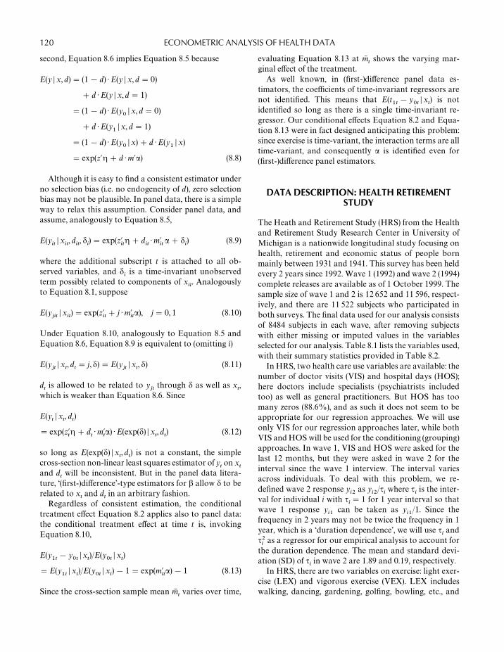
second, Equation 8.6 implies Equation 8.5 because

E(y �x, d) � (1 � d) ·E(y �x, d� 0)

� d ·E(y � x,d� 1)

� (1 � d) ·E(y��x, d� 0)

� d ·E(y��x, d� 1)

� (1 � d) ·E(y��x) � d ·E(y

�� x)

� exp(z�� d ·m��) (8.8)

Although it is easy to find a consistent estimator underno selection bias (i.e. no endogeneity of d), zero selectionbias may not be plausible. In panel data, there is a simpleway to relax this assumption. Consider panel data, andassume, analogously to Equation 8.5,

E(y��x

�, d

�, �

�) � exp(z�

�� d

�·m�

��

�) (8.9)

where the additional subscript t is attached to all ob-served variables, and �

�is a time-invariant unobserved

term possibly related to components of x�. Analogously

to Equation 8.1, suppose

E(y��

�x�) � exp(z�

�� j ·m�

��), j� 0, 1 (8.10)

Under Equation 8.10, analogously to Equation 8.5 andEquation 8.6, Equation 8.9 is equivalent to (omitting i)

E(y��x

, d

� j, �) �E(y

��x

, �) (8.11)

dis allowed to be related to y

�through � as well as x

,

which is weaker than Equation 8.6. Since

E(y� x

, d

)

� exp(z�� d

·m�

�) ·E(exp(�) � x

,d

) (8.12)

so long as E(exp(�) � x,d

) is not a constant, the simple

cross-section non-linear least squares estimator of yon x

and d

will be inconsistent. But in the panel data litera-

ture, ‘(first-)difference’-type estimators for � allow � to berelated to x

and d

in an arbitrary fashion.

Regardless of consistent estimation, the conditionaltreatment effect Equation 8.2 applies also to panel data:the conditional treatment effect at time t is, invokingEquation 8.10,

E(y�

� y�

�x)/E(y

��x

)

�E(y�

�x)/E(y

��x

) � 1 � exp(m�

��) � 1 (8.13)

Since the cross-section sample mean m�varies over time,

evaluating Equation 8.13 at m�

shows the varying mar-ginal effect of the treatment.

As well known, in (first-)difference panel data es-timators, the coefficients of time-invariant regressors arenot identified. This means that E(t

�� y

��x

) is not

identified so long as there is a single time-invariant re-gressor. Our conditional effects Equation 8.2 and Equa-tion 8.13 were in fact designed anticipating this problem:since exercise is time-variant, the interaction terms are alltime-variant, and consequently � is identified even for(first-)difference panel estimators.

DATA DESCRIPTION: HEALTH RETIREMENTSTUDY

The Heath and Retirement Study (HRS) from the Healthand Retirement Study Research Center in University ofMichigan is a nationwide longitudinal study focusing onhealth, retirement and economic status of people bornmainly between 1931 and 1941. This survey has been heldevery 2 years since 1992. Wave 1 (1992) and wave 2 (1994)complete releases are available as of 1 October 1999. Thesample size of wave 1 and 2 is 12 652 and 11 596, respect-ively, and there are 11 522 subjects who participated inboth surveys. The final data used for our analysis consistsof 8484 subjects in each wave, after removing subjectswith either missing or imputed values in the variablesselected for our analysis. Table 8.1 lists the variables used,with their summary statistics provided in Table 8.2.

In HRS, two health care use variables are available: thenumber of doctor visits (VIS) and hospital days (HOS);here doctors include specialists (psychiatrists includedtoo) as well as general practitioners. But HOS has toomany zeros (88.6%), and as such it does not seem to beappropriate for our regression approaches. We will useonly VIS for our regression approaches later, while bothVIS and HOS will be used for the conditioning (grouping)approaches. In wave 1, VIS and HOS were asked for thelast 12 months, but they were asked in wave 2 for theinterval since the wave 1 interview. The interval variesacross individuals. To deal with this problem, we re-defined wave 2 response y

��as y

��/�

�where �

�is the inter-

val for individual i with �� 1 for 1 year interval so that

wave 1 response y��

can be taken as y��

/1. Since thefrequency in 2 years may not be twice the frequency in 1year, which is a ‘duration dependence’, we will use �

�and

��

as a regressor for our empirical analysis to account forthe duration dependence. The mean and standard devi-ation (SD) of �

�in wave 2 are 1.89 and 0.19, respectively.

In HRS, there are two variables on exercise: light exer-cise (LEX) and vigorous exercise (VEX). LEX includeswalking, dancing, gardening, golfing, bowling, etc., and


Table 8.1 Variables (other than responses and exercises)

�: Interval between interviews (years)Age (year) J1: Managerial specialty operationMarried (1, 0) J2: Professional specialty operation and technical supportJob dummy (1, 0) J3: SalesWork hour (per week) J4: Clerical, administrative supportIncome ($1000) J5: Service: private household, cleaning, buildingSchooling (year) J6: Service: protectionMale (1, 0) J7: Service, food preparationRace (1, 0): Rc1: white J8: Health services

Rc2: black J9: Personal servicesRc3: Asian J10: Farming, forestryRc4: Hispanic J11: Mechanics and repairR54: Native American J12: Construction trade and extractors

Hypertension (1, 0) J13: Precision productionDiabetes (1, 0) J14: Operators: machineLung diseases (1, 0) J15: Operators: transport, etc.Heart diseases (1, 0) J16: Operators: handlers, etc.Emotion/Nerve problem (1, 0) J17: Member of armed forcesArthritis/Rheumatism (1, 0) Health insurance (1, 0): H1: MedicarePain (1, 0) H2: MedicaidResidence (1, 0): Rs1: New England H3: CHAMPS/VA

Rs2: Middle Atlantic H4: Other government planRs3: East North Central H5: Group insuranceRs4: West North CentralRs5: South AtlanticRs6: East South CentralRs7: West South CentralRs8: MountainRs9: Pacific

VEX includes aerobics, running, swimming, bicycling,etc. The question on exercise in wave 1 asks the frequencyfor the last 12 months in five categories:

Never, less than once a month,

1—3 times a month,

1—2 times a week, 3 or more a week

The question in wave 2 asks the frequency for theinterval since the wave 1 interview: ‘How often do youparticipate in physical activity?’ and ‘What interval wasthat?’ We converted the frequency here into one appro-priate for the five categories. But then we found that somecategories are not well defined with too few observations,and that people change their exercise habits too muchacross two waves, which may be a recollection error.Given below are the transition probabilities for exercise:in a given row, the transition probabilities from a givenexercise category at wave 1 to the categories at wave 2 arepresented (thus, the sum in a given row in one):

LEX transition matrix

t� 1�t�2 0 1 2 3 4

0 0.433 0.019 0.081 0.136 0.3311 0.212 0.059 0.184 0.171 0.3732 0.130 0.041 0.165 0.234 0.4293 0.084 0.012 0.126 0.265 0.5134 0.061 0.005 0.045 0.165 0.723

VEX transition matrix

t� 1�t�2 0 1 2 3 4

0 0.626 0.044 0.151 0.079 0.0991 0.423 0.083 0.248 0.137 0.1092 0.282 0.055 0.323 0.213 0.1273 0.232 0.036 0.258 0.287 0.1874 0.195 0.027 0.123 0.273 0.381


Table 8.2 Summary statistics for variables

Wave 1 Wave 2

Mean SD Min. Med. Max. Mean SD Min. Med. Max.

HOS 0.60 3.40 0 0 91 0.65 2.88 0 0 76VIS 3.64 6.01 0 2 80 3.34 4.91 0 2 78� (interview interval) 1 0 1 1 1 1.89 0.19 1.31 1.88 2.60

LEX 0.75 0.44 0 1 1 0.78 0.41 0 1 1VEX 0.24 0.43 0 0 1 0.30 0.46 0 0 1

Age 55.31 5.49 23 55 82 57.31 5.49 25 57 84Married 0.83 0.38 0 1 1 0.81 0.39 0 1 1Job dummy 0.69 0.46 0 1 1 0.64 0.48 0 1 1Work hour 27.88 21.38 0 40 95 25.52 21.79 0 35 95Income 55.72 48.78 �1.08 46 625.2 60.03 87.20 �4.9 42.28 1570Schooling 12.19 3.18 0 12 17 12.19 3.18 0 12 17Male 0.46 0.50 0 0 1 0.46 0.50 0 0 1

Hypertension 0.36 0.48 0 0 1 0.41 0.49 0 0 1Diabetes 0.10 0.30 0 0 1 0.12 0.32 0 0 1Lung diseases 0.07 0.26 0 0 1 0.09 0.28 0 0 1Heart diseases 0.11 0.31 0 0 1 0.14 0.35 0 0 1Emotion/Nerve 0.10 0.29 0 0 1 0.13 0.33 0 0 1Arthritis/Rheumatism 0.36 0.48 0 0 1 0.44 0.50 0 0 1Pain 0.23 0.42 0 0 1 0.25 0.43 0 0 1

H1 0.06 0.23 0 0 1 0.09 0.29 0 0 1H2 0.03 0.17 0 0 1 0.04 0.19 0 0 1H3 0.05 0.22 0 0 1 0.05 0.22 0 0 1H4 0.00 0.07 0 0 1 0.01 0.10 0 0 1H5 0.72 0.45 0 1 1 0.72 0.45 0 1 1

LEX� 1 and VEX� 1 columns have too small probabil-ities compared with the other columns. Also, the tablesshow too much variation in exercise habits over 2 years.

Facing these problems, we converted the five categoriesinto two: (0, 1, 2) becomes 0 while (3, 4) becomes 1; it maytake at least once a week frequency for the exercises to beeffective. With the conversion, 75% (24%) of the peopledo LEX (VEX) in wave 1, and the new transition matricesare:

LEX: (0, 1, 2) to 0, (3, 4) to 1

t� 1�t� 2 0 1

0 0.438 0.5621 0.144 0.856

VEX: (0, 1, 2) to 0, (3, 4) to 1

t� 1�t� 2 0 1

0 0.786 0.2141 0.423 0.577

One should not be too wary of this construction of thedummy variables: we are merely redefining LEX andVEX as ‘doing exercise at least once a week’. Had weconstructed the dummy variables differently, we would bedefining LEX and VEX (i.e. the treatments) differently,and consequently measuring the effects of different treat-ments. For instance, if we define exercise as at least once amonth, we should transform the five categories into twoby (0, 1) to 0 and (2, 3, 4) to 1, in which case the transitionmatrix becomes

LEX: (0, 1,) to 0, (2, 3, 4) to 1

t� 1�t� 2 0 1

0 0.369 0.6311 0.086 0.914

VEX: (0, 1,) to 0, (2, 3, 4) to 1

t� 1�t� 2 0 1

0 0.620 0.3801 0.267 0.733


Here, the right-most columns have more probabilitymasses than those in the preceding two matrices, becauseexercise� 1 becomes easier with the ‘easier’ transform-ation. In most of our empirical analysis later, we will usethe dummy variables (0, 1, 2) to 0 and (3, 4) to 1; when wepresent regression results, we will show the estimates forthe other dummy variables ((0, 1) to 0 and (2, 3, 4) to 1) aswell.

Turning to the other variables, the average age of wave1 is 55.31 indicating an old population; we added two tothe first wave age to get the second wave age, because theactual second wave age that depends on the interviewdate was not available. The age in wave 1 ranges from23—82 because the respondents include spouses and part-ners. The majority of the respondents are married: 83 and81% in wave 1 and wave 2, respectively.

We use job dummy, work hour, income and job title (17categories) as job-related variables. Simply having a jobor not may matter, say for mental health and for stayingactive. A high work-hour means less chance to visit doc-tors; the average work-hour per week among the workersin wave 1 is 27.88 while the national average is 34.8(Bureau of Labor Statistics). Income includes all kinds ofhousehold income, not only wage and pension but alsocapital gain (or loss); the average household income andthe median is $57 877 and $44 220, respectively. Job cate-gories matter for health care demand; e.g. blue-collarworkers are subject to higher risk for job-related injuries.For confidentiality, however, job categories in HRS havebeen aggregated and available only in 17 categories; theirsummary statistics are omitted to save space.

Schooling, top-coded at 17, shows the highest gradecompeted; it is time-invariant in our data. There are 3906males and 4578 females. The race variable consists of fivecategories: ‘White’, ‘Black’, ‘Asian or Pacific Islander’,‘Hispanic’ and ‘American Indian or Alaskan Native’. Themajority in the samples is White (74%), followed by Black(15%), Hispanic (9%), Asian (1%) and American Indian(1%). The proportions are not too far from the censusproportions: according to 1997 US Bureau of Census,they are 72.6%, 12.1%, 11.0%, 3.6% and 0.7%, respect-ively.

There are a large number of diseases and it is impossi-ble to know exactly what kind of disease each respondenthas. Hypertension, diabetes, lung diseases, heart diseases,emotion/nerve problems, arthritis/rheumatism and painare used as disease variables. Lung disease dummy in-cludes chronic bronchitis and emphysema. Heart diseasedummy includes heart attack, coronary heart disease,angina and congestive heart failure. Emotion/nervedummy includes emotional, nervous and psychiatricproblems. Those who have a cancer or experienced astroke are removed from the data, because they may be

too different in terms of health care demand from the restof the population (admittedly, this decision is somewhatarbitrary). All disease variables show whether one hasever gotten the disease or not; using ever variables insteadof the current status alleviates the endogeneity problem ofthe disease variables. All disease variables increase overtime. Smoking variables are available, but unreliable: thepast smokers show the maximum number of cigarettesper day and how long ago they quit, whereas the currentsmokers show only the average number of cigarettes perday but not when they started smoking. Thus, those whotried smoking only once in a high school day and quit onthe same day has the maximum smoking equal to one,which is also the case for a regular smoker smoking onecigarette per day. Smoking will not be used in our empiri-cal analysis.

Health care demand may be affected by residence be-cause each state has its own health care policy. For confi-dentiality, however, the residence variables in HRS havebeen aggregated to 11 regions, two of which have norespondents: ‘US NA state’ and ‘Not in a Census Divi-sion’. The remaining nine regions are shown in Table 8.1.The residence is available only in wave 1; in wave 2, thereis a question whether the respondent has moved sincewave 1 interview; less than 10% answered yes. But it isunlikely that many of them moved out of their regions.For these reasons, we treat residence as time-invariant.To save space, summary statistics for residence are omit-ted.

Health insurance matters for health care. About 16%of the subjects are covered by public health insurance:Medicare (for the old and the handicapped), Medicaid(for the poor) and CHAMPS/VA (for military retirees).About 72% are covered by insurance bought throughtheir or their partner’s companies or unions.

REGRESSION ESTIMATORS

In this section, we describe the regression estimators usedin this paper; more discussion can be found, e.g. inCameron and Trivedi [8] and Lee [9]. First, cross-sectionregression estimators are presented, pooling two wavesinto one big cross-section, which entails that indepen-dence assumption across observations may fail. This isoften called a ‘group structure’ problem: each individualis a group with two observations possibly related to eachother. Second, panel regression estimators are described.In the literature, two strains of panel estimators are avail-able: ‘random-effect’ and ‘fixed-effect’; we will use only thelatter in this paper, for it allows relationships between atime-invariant error �

�and regressors while the former

does not unless strong parametric assumptions are in-


voked. Allowing the relationships is our only routethrough which regressor endogeneity issue is addressed.Although all methods described in this section were ap-plied to our data, only about half the results will bereported later for different reasons.

Let y�

be the observed count response variable forindividual i at time t. Poisson regression specifies that y

�given x

�is drawn from Poisson(�

�), where

�� exp(x�

��) (8.14)

x�

is a k�� 1 vector of regressors, and Poisson(�

�) de-

notes Poisson distribution with parameter ��; the prob-

ability of y�

given x�

is given by

f (y�� x

�) �

exp(��)��

�y�!

, y�� 0, 1, 2, . . .

Further assuming that (y�, x�

�)�, t� 1, 2, i� 1, . . .,N are

iid (independent and identically distributed), the Poissonmaximum likelihood estimator (MLE) maximizes thelog-likelihood function:

��

��

[ � ln(y�!) � exp(x�

��) � y

�x��] (8.15)

the first derivative is

��

��

�y�� exp(x�

��))�x

�(8.16)

The Poisson MLE includes the restriction

E(y��x

�) � V(y

��x

�) ��

�

In reality, the conditional variance often tends to bebigger than the conditional mean; this is called an ‘over-dispersion’ problem. Ignoring this problem renders toosmall standard errors. Since Equation 8.16 � 0 is asample moment condition, the estimator using Equation8.16� 0 only under E(y

��x

�) ��

�without specifying the

likelihood is a method of moment estimator (MME); wewill use this MME, not the Poisson MLE. The MMEdoes not require the iid assumption across t, while thePoisson MLE requires iid across t as well as i. In theMME, the asymptotic variance is to be estimated by

��

�s�(�)/�b�

�· �

�

s�(�)s�

�(�) ·��

�

�s�(�)/�b��

�,

not by �� s�(�)s��(�)�

�(8.17)

where s�(b) � �

��y

�� exp(x�

�b)�x

�.

One way to allow for over-dispersion while stayingwithin MLE framework is introducing unobserved het-erogeneity, say �

�. Suppose y

�� (x

�, �

�) follows Pois-

son(��),

�� exp(x�

��

�)

exp(��) �x

�follows �(

�,

�),

�� (1/�)�

�k, � 0, where

�(a, b) denotes � distribution with parameters a and b, and� and � are parameters to estimate, while k is typically setat 0 or 1. With �

�integrated out, y

�� x

�follows a negative

binomial distribution with parameters �/(�

��

�) and

�

(denoted as NB(�/(�

��

�),

�)): for �(s) �

�

�

z��edz with s 0,

f (y�� x

�) � [�(y

��

�)/��(

�)�(y

�� 1)�]

· ��/(�

��

�)�

� · ��/(�

��

�)��

NB with k� 1 (k� 0) is called NB1 (NB2). This distribu-tion allows over-dispersion:

E(y��x

�) ��

�and V(y

��x

�) � �

��

�

The variance is linear in ��

if k� 1, and quadratic ifk� 0, which explains the names NB1 and NB2; eitherway, the variance is greater than the mean. For NB1,�/(�

��

�) � 1/(1 ��) is a constant between 0 and 1;

for NB2, �/(�

��

�) is not a constant but

�� 1/� is.

The Poisson MLE is included as a limiting case when�� 0� since E�exp(�

�) �x

�� 1 and V�exp(�

�) �x

��

��

.Assuming that (y

�, x�

�)�, t� 1, 2, i� 1, . . .,N are iid, the

NB log-likelihood function to maximize for � and � is

��

��

[ln(�(y��

�)) � ln(�(

�)) � ln(�(y

�� 1))

��(ln(

�) � ln(�

��

�))

� y�(ln(�

�) � ln(�

��

�))]

There are different ways to parametrize NB (e.g. Win-kelmann and Zimmermann [10]), and we followed Deband Trivedi [11]. For our empirical analysis later, we willreport the NB2 result, but not the NB1, for the maximizedlog-likelihood value was bigger for NB2. Since NB2 isbased upon stronger assumptions than the MME, we willfocus on the MME when we interpret our empirical find-ings.


One problem with cross-section analysis is that theremay be an unobserved variable related to regressors andthe response variable at the same time, which renderscross-section estimates inconsistent in general unless theunobservable variable is integrated out as in NB1 in afully parametric framework. For example, some peopletend to be (genetically) weak or always worrying that theyuse health care more often than others; such genetic factoror tendency can be related to regressors. Those unobser-ved components, if time-invariant as genes, can be con-trolled for (i.e. eliminated) if panel data is used: the basicidea is to first-difference the model (or variables) to elim-inate them. For count responses, the so-called ‘condi-tional Poisson’ (Hausman et al. [12]), being a panel ver-sion of the cross-section Poisson, does this task. Theunobserved time-invariant variable �

�, is often called

‘fixed-effect’, ‘unit-specific effect’ or ‘related-effect’ is theliterature; following Lee [13], we will adopt the last ex-pression ‘related-effect’ for �

�from now on. There can be

other sources of endogeneity, say through a time-varianterror, but the methods to be used in this paper cannotdeal with them; the latent-variable-based approach toallow for endogeneity in Lee [14] and a related one in Lee[15] are, in general, not applicable for count responses(see also Windmeijer and Santos-Silva [16]).

In addition to the iid assumption across i, imposingtwo assumptions that

y��

, . . ., y�

are independent of one another

given x��

, . . .,x�

, ��, and y

�� (x

�, �

�)

follows Poisson (exp(x��

�)) (8.18)

the conditional Poisson log-likelihood function to bemaximized for � is

��ln��

��

y�� !��

��

ln(y�!)

� ��

y��x�� ln�

��

exp(�x��

�)�� (8.19)

where �x��

�x�� x

��. The two assumptions listed

ahead are the restrictive features of the conditional Pois-son.

Still maintaining the iid assumption across i, Hausmanet al. [4] assume

y��

, . . ., y�

are independent of one another

given x��

, . . .,x�

, ��, and y

�� (x

�, �

�)

follows NB(p�, exp(x�

��

�)) for some p

�(8.20)

to relax the Poisson part in the conditional Poisson; sincethe first parameter p

�is time-invariant, the NB here is of

type NB1. The resulting ‘conditional negative binomial’log-likelihood function to be maximized for � is (both p

�and �

�drop out in the conditioning)

��

��

�ln �(�� y

�) � ln �(�

�) � ln �(y

�� 1)�

� ln ��

�� ln ��

��

y�� 1�

� ln ��

��

��

y��

Wooldridge [17] shows that the conditional Poisson’srestrictive assumption can be relaxed considerably. Sup-pose

E(y��x

��, . . .,x

� ,�

�) �E(y

��x

�, �

�)

� exp(x��

�)

where the first equality is ‘strict exogeneity’. So long asthis holds (along with minor regularity conditions), maxi-mizing the conditional Poisson maximand Equation 8.19

yields a �N-consistent estimator for �. This ‘quasi-con-ditional MLE (QCL)’ allows dependence amongy��

, . . ., y�

given x��

, . . ., x�

, ��, relaxing Equation 8.18.

The asymptotic variance of QCL can be estimated analo-gously to Equation 8.17 with s

�denoting the score func-

tion. QCL may be taken as a panel version of the MMEfor the Poisson MLE. Since QCL is based upon theweakest assumptions yet while allowing for a related-effect, we take QCL as our main estimator.

It is not known whether analogous relaxation of as-sumption is possible for the conditional negative bi-nomial. For our empirical analysis, conditional negativebinomial converged not as well as QCL, and when it did,it returned implausible values (with most absolute t-values running over 50). For these two reasons, the condi-tional negative binomial will not be reported later for ourempirical analysis.

RESULTS OF CONDITIONINGAPPROACHES

In this section, we present our empirical analysis withoutusing the exponential regression function. Here, covari-ates are controlled for by conditioning, and the variableof interest (exercise) is used for grouping; inferences can be


Table 8.3 Results of conditioning and pooled-data

A. LEX and VIS

VIS�LEX 0: Seldom do 1: Do Sum

0 89 (0.366) 241 (0.237) 330 (0.262)1—5 140 (0.576) 723 (0.711) 863 (0.685)6— 14 (0.058) 53 (0.052) 67 (0.053)Sum 243 (1.000) 1017 (1.000) 1260 (1.000)Test statistic: 17.831

B. VEX and VIS

VIS�VEX 0: Seldom do 1: Do Sum


C. LEX and HOS

HOS�LEX 0: Seldom do 1: Do Sum


D. VEX and HOS

HOS�VEX 0: Seldom do 1: Do Sum


then drawn from differences between the groups withdifferent exercise habits. The advantage of this condition-ing approach is that there is no need to specify the re-gression functional form nor distributions for the modelerror terms. But a disadvantage is that we cannot controlfor too many variables; if we do, there will be too fewobservations left for the groups. Not being able to controlfor all relevant variables means the risk of omitted vari-able bias. In the following section, we present regressionapproaches that can control for many covariates; butthen, there will be the risk of misspecified models. An-other disadvantage of the conditioning approach is thatwe will be learning only about the selected sub-popula-tion, and there is no guarantee that the findings from thesub-population can be applied to the other sub-popula-tions. Despite this, since the effects of exercise are a con-cern for everybody, not just for old people, we will extracta sub-population representing relatively younger andhealthier group and analyse them.

The following is for the average health care demandacross exercise habits using all observations:

LEX � 0 LEX � 1 VEX� 0 VEX � 1

HOS 0.982 0.514 0.712 0.388VIS 4.120 3.293 3.707 2.896

People who do exercise, LEX or VEX, having lowerhealth care demand. But since exercising people maydiffer from non-exercising people in other variables, thistable does not show that the differences in health caredemand are due to differences in exercise habits.

To better control for covariates and get a homogenousgroup of people, we select a healthy sub-population withage 50—57 in wave 1 and the following characteristicsholding for both waves: married, all zero disease dum-mies, no pain, working, no public health insurance, andgroup insurance dummies being one. To the extent thatthe unobserved variables are related to these covariates,the unobserved variables and partially controlled for aswell. Given that we are looking at an old population, thefindings from this healthy sub-population stands a betterchance to be applicable to young and healthy people,which was the main motivation to look at the particularsub-population as already mentioned. The sample size ofthe sub-population is 1260 (630

�� 2

��) in the

pooled data.Table 8.3 consists of four 3 � 2 contingency panels

showing the absolute frequencies and the relative fre-quencies in a given column; at the bottom right of eachpanel is the Pearson � test statistic; for the 3 � 2 classifi-cation, the critical value for the test is 6.0 at size 5%.Looking at the test statistics and the relative frequencies,

independence between VIS and LEX is rejected in the firstpanel while we fail to reject independence in the otherpanels. The relative frequencies however show that, ifanything, LEX increases both VIS and HOS, contrary tothe message of the above simple table with no covariatescontrolled for; the effects of VEX are not clear. We canthink of some reasons for this surprising finding: en-hanced health-awareness, exercise under doctors’ super-vision, and the reverse causal effect of more exercise fol-lowing doctor visits or hospitalization.

The preceding analysis is of cross-section type. To take


Table 8.4 Exercise change and health care demand change

A. LEX and VIS changes

VIS-change�LEX change 0—0 0—1 1—0 1—1 Sum

Decreased 16 (0.308) 21 (0.276) 17 (0.270) 130 (0.296) 184 (0.292)Same 17 (0.327) 20 (0.263) 21 (0.333) 139 (0.317) 197 (0.313)Increased 19 (0.365) 35 (0.461) 25 (0.397) 170 (0.387) 249 (0.395)Sum 52 (1.000) 76 (1.000) 63 (1.000) 439 (1.000) 630 (1.000)

B. VEX and VIS changes

VIS-change�VEX change 0—0 0—1 1—0 1—1 Sum


C. LEX and HOS changes

HOS-change�LEX-change 0—0 0—1 1—0 1—1 Sum


D. VEX and HOS changes

HOS-change�VEX-change 0—0 0—1 1—0 1—1 Sum


advantage of panel data, now we look at changes inexercise habits and health care demand over two waves. Ifa linear model were used, this would amount to first-differencing the model to get rid of all time invariants,which then would not affect analysis based on changes.Table 8.4 lists four panels, analogously to Table 8.3.There are four types of LEX or VEX across two waves:0—0, 0—1, 1—0, and 1—1. VIS and HOS are now classifiedinto three: decrease, the same and increase. In Table 8.5,many Pearson � test statistics are presented. For in-stance, the entry at row 0—1 and column 0—0 of panel A is1.202, which is the test statistic for the 3 � 2 contingencypanel consisting of panel A of Table 8.4 with all rows andonly two columns for 0—0 and 0—1.

In Table 8.5, there are four numbers greater than thecritical value 6 at 5%, but all four are for HOS. In panelC, the first significant number 6.151 is based upon too few

observations as can be seen in the corresponding panel Cof Table 8.4, but the second significant number 6.135 (for0—1 and 1—1) is based upon observations not as few, andpanel C of Table 8.4 indicates a positive association be-tween HOS increase and LEX increase. In panel D ofTable 8.5, the first significant number is 6.498 (for 0—0 and1—0), and the corresponding panel D of Table 8.4 showsboth decrease and increase in HOS, making inferencedifficult. The second significant number in the panel D ofTable 8.5 is 8.158 for 1—0 and 1—1, but judging from thecorresponding panel D of Table 8.4, the number is basedupon too few observations.

In short, for the healthy sub-population with somecovariates controlled for, there is a positive associationbetween LEX and both VIS and HOS. For the samesub-population, looking at changes over time, we have apositive association between LEX and HOS changes.


Table 8.5 Test statistics for exercise change and health caredemand change

0—0 0—1 1—0

A. LEX and VIS changes0—1 1.202 — —1—0 0.219 0.904 —1—1 0.094 1.561 0.191

B. VEX and VIS changes0—1 2.450 — —1—0 0.869 3.502 —1—1 2.282 2.068 2.761

C. LEX and HOS changes0—1 6.151 — —1—0 4.386 4.545 —1—1 0.480 6.135 4.481

D. VEX and HOS changes0—1 0.057 — —1—0 6.498 3.354 —1—1 4.284 3.775 8.158

These findings are in sharp contrast to the message of thecrude table with no covariates controlled for, and theysuggest that the healthy sub-population and the remain-ing (unhealthy) sub-population may differ in terms ofexercise effects on health care demand.

Since the above tables are based only upon 630 � 2cases, now we enlarge the healthy sub-population byselecting the individuals from the pooled data with zerodisease dummies (all six of them) and zero pain dummy(insurance, working, and marriage are not controlled fornow). Defining h

�� 1 if healthy and 0 otherwise accord-

ing to this definition, we get P(h� 1) � 0.288, and

E(y � LEX � 0, h� 0) � 4.815

E(y � LEX � 1, h� 0) � 3.858

E(y � LEX � 0, h� 1) � 1.433

E(y � LEX � 1, h� 1) � 1.643

considerably more information may lurk in � for health,but � is not observed and hence cannot be used for h. Thenumbers show that, for the healthy sub-population, LEXis indeed positively associated with y; for the unhealthysub-population, LEX is negatively associated with y.Since the proportion of the healthy sub-population is low(0.288), the unhealthy sub-population effect dominates toresults in the first simple table of this section.

RESULTS OF REGRESSION APPROACHES

In the preceding section, we showed our conditioningapproaches for a healthy sub-population. In this section,we present three sets of regression model estimates:MME, NB2 and QCL, where MME and NB2 are forpooled cross-sections while QCL is for panel. As men-tioned already, we use only VIS as health care demand inthis section, since HOS has too many zeros. Thanks to theadvantages of panel related-effect methods, QCL pro-vides the most robust conclusions in the regression ap-proaches, followed by MME, which is based upon as-sumptions weaker than those for NB2. NB2 results areprovided (but de-emphasized) only for the sake of com-parison; we will not mention NB2 any further other thannoting here that they are close to the MME estimates.

Table 8.6 shows the estimates and the t-values obtainedwith the main exercise dummies, whereas Table 8.7 showsthose with the ‘easy’ exercise dummies constructed fromthe original five categories as (0, 1) to 0 and (2, 3, 4) to 1; wewill focus on Table 8.6. To save space, the estimates forthe residence and job-dummies are omitted. As a refer-ence, the last rows of Tables 8.6 and 8.7 show the maxi-mized log-likelihood function values; for MME, it is thePoisson log-likelihood at MME, and for QCL, it is theconditional Poisson log-likelihood at QCL; constantsirrelevant for maximization in those log-likelihoods arenot included in the reported maximand values.

In Table 8.6, � and �� look insignificant for MME. Butwe easily reject insignificance of � and ��, because theWald test statistic value is 126.4 with the p-value 0.000.When only � is included in the MME model, the coeffi-cient (t-value) for � is �2.73 (�11.56), meaning negativeduration dependence. This shows that the small t-valuesfor � and �� in MME are due to a high correlationbetween � and ��. In QCL however, the duration effect ispositive, contradicting the negative effect in MME.

Both LEX and VEX look insignificant in MME andQCL, but this is misleading, because some interactionterms (e.g. heart disease-LEX in MME and QCL, andemotion/nerve-VEX in QCL) are significant; so long asthere is at least one significant interaction term, LEX andVEX are significant. The marginal effects for wave 1 andwave 2 are in the following table where Lower (Upper)stands for the lower (upper) bound for the 95% confi-dence interval, Effect is the desired marginal effect, andthe numbers in (·) are the arithmetic mean effects Equa-tion 8.3 provided here without confidence intervals onlyfor the sake of comparison:


MME Lower Effect Upper QCL Lower Effect Upper

LEX LEXt� 1 �0.068 �0.027 (�0.024) 0.015 t� 1 �0.026 0.031 (0.034) 0.089t� 2 �0.068 �0.027 (�0.023) 0.015 t� 2 �0.025 0.031 (0.035) 0.089

VEX VEXt� 1 �0.021 �0.010 (�0.009) 0.002 t� 1 �0.027 �0.010 (�0.009) 0.006t� 2 �0.027 �0.013 (�0.012) 0.002 t� 2 �0.033 �0.013 (�0.011) 0.006

MME Lower Effect Upper QCL Lower Effect Upper

LEX LEXt� 1 �0.119 �0.063 (�0.055) �0.006 t� 1 �0.037 0.044 (0.050) 0.128t� 2 �0.118 �0.063 (�0.053) �0.007 t� 2 �0.027 0.052 (0.060) 0.134

VEX VEXt� 1 �0.037 �0.022 (�0.021) �0.007 t� 1 �0.035 �0.014 (�0.014) 0.007t� 2 �0.055 �0.034 (�0.033) �0.012 t� 2 �0.050 �0.021 (�0.020) 0.010

None of the effects is significant. But looking at the esti-mates and the interval sizes on the positive and negativesides, we can say that LEX has a small negative effect ofaround �3% in MME and a small positive effect ofaround 3% in QCL, whereas VEX has a small negativeeffect of around �1% in both MME and QCL. Thearithmetic mean effects are little different from the geo-metric mean effects. The effects do not change much overtime; for a longer panel, the time-varying pattern of theeffects would be more interesting.

How do we reconcile the difference between MME andQCL for LEX? Suppose �

�is the unobserved trait affected

by LEX; here we regard ��

as unobserved health stockbuilt long-term. And recall our discussion on short-termand long-term effects in the Introduction. According tothe discussion, the panel estimate shows the short-termeffect of LEX, while the cross-section estimate is a long-term affect consisting of the short-term effect and theeffect through �

�. The reconciliation is as follows. In the

short run, with both observed health and unobservedhealth controlled for by the regression method and re-lated-effect, respectively, LEX increases VIS by about 3%perhaps due to consulting doctors or enhanced healthconcern. But doing LEX for a long time will decrease VISby about 6% perhaps due to improved health which canbe a result of LEX itself as well as other adopted healthylife style going along with LEX. This negative effect can-cels the short-term positive effect to result in the long-term effect, which is �3%. One caution is that, for theinterpretation of �

�as unobserved health stock to be

coherent, we would expect a difference between short-runand long-run effects for VEX, but the table shows theidentical numbers, which may be due to the statistical

insignificance; in the table presented below however, VEXis seen to have different short-run and long-run effects.

Now we turn to the estimates of MME and QCL otherthan those for LEX and VEX. Among the estimates sig-nificant for both MME and QCL (hypertension, lungdisease, pain and heart-disease-LEX), the signs all agree,and only the magnitude of pain in MME is twice as big asthat in QCL; the other magnitudes are close. As differ-ence-type panel estimators typically have small absolutet-values, QCL’s t-values are mostly smaller than those ofMME; the only variable that is significant in QCL butnot in MME is emotion/nerve-VEX (and diabetes-VEX).In fact, the interaction terms with VEX are all insignifi-cant other than emotion/nerve-VEX in QCL.

Age increases y in MME while decreasing y in QCL. Ifwe still interpret � as unobserved health stock, then withobserved and unobserved health cotrolled for, there is noreason to believe that age should increase y. Marriage hasa negative effect, but insignificant and small in its magni-tude. Schooling has a significant positive effect, possiblyreflecting health awareness aspect. Men demand substan-tially lower health care than women, which is an almostuniversal phenomenon. All disease variables increase yother than the insignificant estimate for diabetes in QCL.Heart-disease-LEX increases y, probably because heartconditions require a doctor’s supervision for exercise.Most health insurance variables increase y in MME whilethey are all insignificant in QCL with mixed signs.

In Table 8.7, we present the results of the same analysisbut with the easy exercise dummies constructed from thefive categories as (0, 1) to 0 and (2, 3, 4) to 1. Tables 8.6 and8.7 are little different other than in some interactionterms. The marginal treatment effects are:


Table 8.6 Estimation with the main exercise dummies

Variables MME (t-value) NB2 (t-value) QCL (t-value)

� 0.748 (69.12)1 0.700 (1.08) 0.680 (1.77)� �0.075 (�0.28) �0.040 (�0.20) 2.548 (1.76)�� 0.066 (�0.75) �0.073 (�1.08) �0.745 (�1.96)LEX �0.023 (�0.51) 0.000 (0.00) 0.068 (1.13)VEX �0.044 (�1.15) �0.024 (�0.96) �0.029 (�0.55)

Age/10 0.297 (1.40) 0.172 (1.35) �3.141 (�1.69)(Age/10)� �0.038 (�1.99) �0.025 (�2.14) 0.042 (0.51)Married �0.050 (�1.58) �0.008 (�0.39) �0.081 (�0.74)Job dummy 0.009 (0.09) �0.005 (�0.08) �0.024 (�0.14)(Work hour)/10 �0.017 (�1.54) �0.012 (�1.63) 0.008 (0.44)ln(income) 0.009 (0.83) 0.009 (1.87) 0.012 (1.00)

Schooling 0.010 (2.15) 0.013 (4.87)Male �0.102 (�3.50) �0.154 (�9.62)White �0.223 (�1.38) �0.145 (�2.18)Black �0.142 (�0.88) �0.067 (�0.98)Hispanic �0.163 (�1.01) �0.114 (�1.62)Asian �0.221 (�1.24) �0.208 (�2.09)

Hypertension 0.301 (6.04) 0.349 (12.67) 0.411 (4.17)Diabetes 0.290 (4.83) 0.353 (8.96) �0.186 (�1.48)Lung disease 0.251 (3.98) 0.288 (6.31) 0.238 (1.91)Heart disease 0.108 (1.66) 0.197 (5.32) 0.098 (0.75)Emotion/nerve 0.211 (3.51) 0.264 (7.30) 0.152 (1.49)Arthritis 0.242 (4.65) 0.234 (8.27) 0.046 (0.52)Pain 0.551 (10.18) 0.604 (21.63) 0.276 (4.67)

Hypertension-LEX �0.008 (—0.15) —0.016 (�0.48) �0.050 (�0.69)Diabetes-LEX 0.051 (0.71) 0.019 (0.39) 0.057 (0.55)Lung disease-LEX 0.060 (0.74) 0.049 (0.89) �0.043 (�0.42)Heart disease-LEX 0.221 (2.93) 0.195 (4.28) 0.200 (2.13)Emotion/nerve-LEX 0.067 (0.90) 0.050 (1.13) �0.091 (�1.01)Arthritis-LEX �0.077 (�1.25) �0.044 (�1.32) �0.013 (�0.18)Pain-LEX �0.106 (�1.60) �0.124 (�3.75) �0.104 (�1.45)

Hypertension-VEX 0.038 (0.74) 0.038 (1.08) �0.054 (�0.79)Diabetes-VEX �0.005 (�0.06) �0.016 (�0.28) 0.205 (1.88)Lung disease-VEX �0.065 (�0.67) �0.013 (�0.17) �0.091 (�0.75)Heart disease-VEX 0.018 (0.25) 0.041 (0.77) 0.131 (1.36)Emotion/nerve-VEX 0.083 (0.96) 0.068 (1.27) 0.309 (2.98)Arthritis-VEX �0.035 (�0.60) �0.049 (�1.41) �0.116 (�1.63)Pain-VEX �0.025 (�0.34) �0.030 (�0.82) �0.051 (�0.61)

H1 0.230 (5.03) 0.280 (9.96) �0.076 (�1.07)H2 0.318 (5.76) 0.346 (8.83) 0.015 (0.15)H3 0.129 (2.50) 0.133 (3.93) �0.120 (�1.08)H4 0.191 (1.83) 0.174 (1.97) 0.041 (0.32)H5 0.149 (4.94) 0.178 (9.95) 0.079 (1.17)

Maximand (no constant) 22 393.825 35 995.033 �39 257.479

The short-term effect of LEX is now about 4—5%, whilethe long-run effect of LEX is about �6% and significant.The VEX effects of minus 2—3% are stronger than in thepreceding table; also differently from the preceding table,the long-run effect of VEX is smaller than the short-run

effect. Collectively, these findings are rather surprising,because the effects are overall stronger despite the weakerdefinition of exercises. Nevertheless, the confidence inter-vals in the two tables overlap, implying that the apparentanomalies fall within the statistical margin of errors. The


Table 8.7 Estimation with the easy exercise dummies

Variables MME (t-value) NB2 (t-value) QCL (t-value)

� 0.745 (69.22)1 0.752 (1.16) 0.749 (1.96)� �0.036 (�0.13) �0.011 (�0.06) 2.637 (1.79)�� 0.076 (�0.85) �0.079 (�1.18) �0.767 (�1.99)LEX �0.052 (�0.90) �0.023 (�0.72) 0.045 (0.58)VEX �0.075 (�2.08) �0.060 (�2.56) �0.057 (�1.17)

Age/10 0.276 (1.30) 0.143 (1.14) �3.126 (�1.66)(Age/10)� �0.036 (�1.89) �0.022 (�1.94) 0.031 (0.38)Married �0.046 (�1.44) �0.001 (�0.07) �0.067 (�0.62)Job dummy 0.010 (0.10) �0.007 (�0.10) �0.017 (�0.11)(Work hour)/10 �0.018 (�1.60) �0.012 (�1.62) 0.004 (0.22)ln(income) 0.011 (0.91) 0.009 (1.89) 0.013 (1.12)

Schooling 0.011 (2.32) 0.014 (5.27)Male �0.105 (�3.64) �0.156 (�9.66)White �0.230 (�1.43) �0.143 (�2.12)Black �0.153 (�0.95) �0.070 (�1.01)Hispanic �0.171 (�1.06) �0.112 (�1.58)Asian �0.247 (�1.38) �0.216 (�2.16)

Hypertension 0.326 (5.13) 0.392 (11.64) 0.393 (3.58)Diabetes 0.182 (2.55) 0.246 (5.21) �0.264 (�1.95)Lung disease 0.181 (2.42) 0.265 (5.12) 0.277 (1.98)Heart disease 0.109 (1.36) 0.220 (5.09) 0.071 (0.51)Emotion/nerve 0.107 (1.53) 0.101 (2.17) 0.121 (1.03)Arthritis 0.270 (4.10) 0.239 (7.04) �0.028 (�0.28)Pain 0.613 (9.01) 0.685 (20.66) 0.332 (4.52)

Hypertension-LEX �0.044 (—0.63) —0.077 (�1.99) �0.029 (�0.34)Diabetes-LEX 0.190 (2.34) 0.170 (3.08) 0.183 (1.68)Lung disease-LEX 0.160 (1.78) 0.095 (1.59) �0.105 (�0.90)Heart disease-LEX 0.199 (2.24) 0.144 (2.80) 0.233 (2.28)Emotion/nerve-LEX 0.208 (2.54) 0.262 (4.98) �0.003 (�0.03)Arthritis-LEX �0.110 (�1.49) �0.051 (�1.31) 0.059 (0.66)Pain-LEX �0.193 (�2.48) �0.233 (�6.15) �0.191 (�2.24)

Hypertension-VEX 0.038 (0.82) 0.051 (1.62) 0.005 (0.08)Diabetes-VEX �0.031 (�0.42) �0.068 (�1.37) 0.044 (0.44)Lung disease-VEX �0.110 (�1.32) �0.085 (�1.34) 0.007 (0.06)Heart disease-VEX �0.002 (�0.03) 0.037 (0.77) 0.028 (0.30)Emotion/nerve-VEX 0.001 (0.02) �0.005 (�0.10) 0.081 (0.83)Arthritis-VEX �0.006 (�0.12) �0.020 (�0.64) �0.026 (�0.41)Pain-VEX 0.017 (0.26) 0.012 (0.35) 0.051 (0.72)

H1 0.221 (4.84) 0.271 (9.66) �0.078 (�1.09)H2 0.328 (5.93) 0.355 (9.11) 0.033 (0.34)H3 0.134 (2.61) 0.138 (4.11) �0.130 (�1.17)H4 0.193 (1.85) 0.176 (2.01) 0.034 (0.27)H5 0.153 (5.06) 0.182 (10.16) 0.081 (1.19)

Maximand (no constant) 22 504.112 36 017.682 �39 280.601

arithmetic means are more different from the geometricmeans than in the preceding table; also the effects aremore time-variant.

Due to lack of instruments for potentially endogenousvariables (e.g., job dummy, income and exercise dummies

can be endogenous), the conclusions drawn in this sectionshould be taken with the limitation of our methods inmind: the endogeneity is allowed as far as it operatesthrough the time-invariant error �

�. To get better answers

to our questions, we need better data; e.g., if there is a


randomized health intervention programme encouragingexercise, the randomization dummy can be an effectiveinstrument for exercise.

CONCLUSIONS

In this paper, we defined and estimated various effects ofexercise (binary treatments) on health care demand(count responses) using a two-wave panel: conditionaland marginal effects, light-exercise and vigorous-exerciseeffects, and short-run and long-run effects. We found thatshort-run light exercise increases health care demand by3—5%, whereas long-run light exercise decreases it by3—6%. Also, short-run vigorous exercise decreases healthcare demand by 1—2%, whereas long-run vigorous exer-cise decreases it by 1—3%. These findings suggest that itwill be hard to reduce health care cost by encouragingpeople to do more exercise; i.e. the health care-cost savingfeature of health intervention programs or campaigns willmaterialize only in the long-run at best.

ACKNOWLEDGEMENTS

The authors are grateful to the editor, two anonymousreferees, Barton Hamilton, Young-sook Kim, John Mul-lahy and Frank Windmeijer for their helpful comments.

REFERENCES

1. Phelps, C.E. Health Economics (2nd edn). Addison-Wesley:Reading, MA, 1997.

2. Leigh, J.P. and Fries, J.F. Health habits, health care use andcosts in a sample of retirees. Inquiry 1992; 29: 44—54.

3. Hofer, T.P. and Katz, S.J. Healthy behaviors among women

in the United States and Ontario: The effect on use of pre-ventive care. Am. J. Publ.Health 1996; 86: 1755—1760.

4. Huijsman, R., Wielink, G. and Rigter, H. Effect van lichaam-sbeweging bij ouderen: een onerzicht can recent literatuur ende mogelijkheid van economische evaluatie. Tijdschr Geron-tol Geriatr 1994; 25: 237—249.

5. Heckman, J.J., Smith, J.A. and Clements, N. Making themost out of program evaluations and social experiments:Accounting for heterogeneity in program impacts. Rev.Econ. Stud. 1997; 64: 487—535.

6. Lee, M.J. Median treatment effect in randomized trials. J. R.Stat. Soc. B 2000; 62: 595—604.

7. Heckman, J.J., Lalonde, R.J. and Smith, J.A. The economicsand econometrics of active labor market programs. InHand-book of Labor Economics, vol. 3, Ashenfelter, A. and Card, D.(eds). Elsevier Science B.V.: Netherlands, 1999; 1865—2087.

8. Cameron, A.C. and Trivedi, P.K. Regression Analysis ofCount Data. Cambridge University Press: Cambridge, 1998.

9. Lee, M.J. Panel Data Econometrics: Methods-of-Momentsand Limited Dependent Variables. Academic Press: SanDiego, CA (in press).

10. Winkelmann, R. and Zimmermann, K.F. Recent develop-ments in count data modelling: Theory and application. J.Econ. Surv. 1995; 9: 1—24.

11. Deb, P. and Trivedi, T.K. Demand for medical care by theelderly: A finite mixture approach. J.Appl. Econom. 1997; 12:313—336.

12. Hausman, J., Hall, B.H. and Griliches, Z. Econometricmodels for count data with an application to the patents —R&D relationship. Econometrica 1984; 52: 909—938.

13. Lee, M.J. A root-N consistent semiparametric estimator forrelated-effect binary response panel data. Econometrica1999; 67: 427—434.

14. Lee, M.J. Semiparametric estimation of simultaneous equa-tions with limited dependent variables: A case study of fe-male labor supply. J. Appl. Econom. 1995; 10: 187—200.

15. Lee, M.J.Method ofMoments and Semiparametric Economet-rics forLimited DependentVariableModels. Springer-Verlag:New York, 1996.

16. Windmeijer, F.A.G. and Santos-Silva, J.M.C. Endogeneityin count data models: An application to demand for healthcare. J. Appl. Econom. 1997; 12: 281—294.

17. Wooldridge, J.M. Distribution-free estimation of some non-linear panel data models. J. Econom. 1999; 90: 77—97.


9

Estimating Surgical Volume – OutcomeRelationships Applying Survival Models:Accounting for Frailty and Hospital Fixed

EffectsBARTONH. HAMILTON1 AND VIVIAN H. HO1,2

�JohnM. Olin School of Business, Washington University in St Louis,MO,USA and �Centre for the Analysisof Cost-Effective Care, Montreal General Hospital, Canada

INTRODUCTION

Past studies have found that patients receiving surgery ina hospital performing a large number of surgeries havebetter outcomes (shorter lengths of stay; lower probabili-ties of in-hospital mortality) than do those undergoingsurgery in a low volume hospital (see Luft et al. [1] for asummary of these studies). These results are particularlypertinent in the context of the current health care debatein many countries. For example, many Canadian prov-inces are being faced with the decision to shut downhospitals and/or reduce the number of hospital beds dueto declining health care budgets. To the extent that thepositive relationship between volume and outcomes isvalid, these governments may actually improve outcomesby regionalizing surgery and closing low volume pro-viders [2].

While the positive volume—outcome relationship hasbeen strongly established, substantial debate exists in theliterature as to the interpretation of this finding. Virtuallyall of the empirical evidence is based on comparisons ofoutcomes between high and low volume hospitals at apoint in time. That is, if hospital A performs more surger-ies than hospital B, outcomes will be better for patientsadmitted to A than for those admitted to B. This relation-ship may reflect a ‘practice makes perfect’ effect in whichhigh volume providers are able to gain expertise in per-forming the procedure, leading to improved outcomes.On the other hand, the relationship between higher vol-

ume and better outcomes may simply represent a ‘selec-tive referral effect’: high quality hospitals which havebetter outcomes, ceteris paribus, are likely to get morereferrals from primary care providers. Consequently,when regressing the outcome measure on surgical vol-ume, the estimated coefficient on surgical volume is likelyto be biased, since volume is a proxy for hospital qualityas well as any practice makes perfect effect. Finally, somehave argued that the positive relationship reflects case-mix differences between low and high volume hospitalsthat are not adequately accounted for in the empiricalanalysis [3].

In the light of this uncertainty regarding interpretation,this paper re-examines the relationship between surgicalvolume and outcomes using longitudinal data on patientsundergoing hip fracture surgery at acute care hospitals inQuebec between 1991 and 1993. Hip fractures are a par-ticularly relevant case study, given that these fractures arethe leading cause of hospitalization for injuries among theelderly [4], and account for a disproportionately largenumber of hospital bed days owing to the relatively longrecovery period associated with hip surgery. In addition,examination of the volume—outcome relationship at Ca-nadian hospitals is particularly timely, since the Cana-dian health care system is currently facing substantialcutbacks and reorganization and most volume—outcomestudies have examined hospitals in the USA. As a result,with few exceptions little is known about the relationshipin Canada [5—7].




Our empirical approach differs from that taken in pre-vious studies, because we attempt to distinguish betweenthe various explanations hypothesized in the literatureconcerning the volume—outcome relationship. First, be-cause the same hospitals are observed over time in thesample, these longitudinal data may be exploited to ac-count for systematic differences in quality between hospi-tals in a very general way using hospital-specific fixedeffects [8]. The period to period fluctuation in the numberof surgical procedures performed at each hospital thenidentifies the effect of volume on outcomes, purged of anydifference in quality across hospitals that is fixed overtime. Our estimates of the volume—outcome relationshipthus rely on the variation in volume and outcomes withinhospitals over time, while almost all previous studies haverelied on variations in volume and outcomes betweenhospitals to estimate the relationship. The results pre-sented in this paper thus relate more closely to one of thekey questions faced by policy makers: what would hap-pen to patient outcomes if the number of surgeries wereincreased (or decreased) at a given hospital?

A second feature of the empirical framework is that theoutcome measures of interest, post-surgery length of stayand inpatient mortality, are allowed to be correlated byestimating a competing risk duration model in which theindividual may be discharged alive or dead. Previousstudies have assumed that these outcomes are indepen-dent. The primary drawback of this assumption is that iflength of stay and in-hospital mortality are not indepen-dent, then one may be more likely to observe an in-hospital death for individuals with long hospital stays. Toaccount for this possibility, the duration model allows forunobserved (to the econometrician) systematic differencesin frailty among patients at the time of admission to thehospital using the non-parametric approach described inHeckman and Singer [9]. Finally, we include much moredetailed controls for patient health status than have typi-cally been used in the literature to account for case-mixdifferences across patients.

Using this empirical methodology, we first estimate aspecification of the volume—outcome relationship whichdoes not control for fixed differences in hospital quality.The estimation results show that higher volume is asso-ciated with an increased conditional (on time in hospital)probability of live discharge, although no significant ef-fect is found on the conditional (on time in hospital)probability of in-hospital mortality. However, when were-estimate the model accounting for fixed quality dif-ferences between hospitals by including hospital-specificdummy variables in the specification, the coefficient onvolume shrinks in magnitude and becomes insignificantlydifferent from zero. Consequently, better patient out-comes in larger hospitals do not appear to be based upon

a volume/learning effect. Rather, the results are moreconsistent with the hypothesis that higher quality hospi-tals are able to draw more patient referrals.

The next section describes the data and presents de-scriptive statistics on the volume—outcome relationship,and the subsequent section outlines the statistical frame-work. We present our results and concluding remarks inthe last two sections.

DATA AND PRELIMINARY EVIDENCE

This paper analyses data from theMED-ICHOdatabase,which contains standardized information from hospitaldischarge abstracts. All acute care hospitals in Quebecreport details of each discharge to the provincialMinistryof Health and Social Services. All patients admitted toacute care hospitals with a primary diagnosis of hip frac-ture (ICD-9 codes 820.0—820.9, fracture of neck of femur;transcervical, pertrochanteric or other unspecified) whowere admitted during or after April 1990 and dischargedbefore March 1993 are included in the sample. Becauseinformation on patients whose hospital stays were still inprogress at the end of March 1993 was unavailable, wemay undercount the volume of surgeries performed inFebruary and March 1993. These patients were thus ex-cluded from the analysis, although the results were vir-tually identical when they were included. Patients admit-ted for revision of prior hip fracture surgery wereexcluded from our sample (1% of original sample). Inaddition, 6% of patients admitted to the hospital with ahip fracture did not undergo surgery. It appears thatmany of these patients were admitted to hospitals that didnot perform hip fracture surgery and then transfixed toanother hospital. Since our goal is to examine the impactof surgical volume on post-surgical length of stay, weexcluded patients not undergoing surgery from the analy-sis.

For each patient, data were obtained on date of surgeryand date and type of discharge (live or dead) and wereused to construct post-surgery length of stay. Informationwas also obtained on other covariates hypothesized toaffect post-surgery mortality and length of stay: age, sex,marital status, type of hip fracture (transcervical, per-trochanteric, other), whether or not the patient was ad-mitted to a teaching hospital, year of admission, medianmale income in postal code of residence and the numberand type of comorbidities at the time of admission.Comorbidities coded as complications were not includedsince these may be endogenous with respect to length ofstay. Information on comorbidities was used to constructa Charlson comorbidity index [10] for each patient usinga codingmethodology developed specifically for adminis-


Table 9.1 Differences in outcomes and case-mix between hospitals, by volume

Averages

Length of Fraction Fraction ofstay died in Number of Charlson hospitals

Average number of (days) hospital comorbidities index universitysurgeries performed (1) (2) (3) (4) affiliated

(Low) �34 31.0 0.094 2.77 0.56 0.29(Average) 34—71 25.9 0.083 2.37 0.55 0.47(High) �71 21.8 0.065 1.90 0.54 0.67

Significance test:p-value� 0.000 0.001 0.000 0.683 0.000

�p-value is from a test of the null hypothesis of equality of means across volume categories.

trative data [11]. This index has been validated as apredictor of mortality in logitudinal studies.

MEASURING HOSPITAL SURGICAL VOLUME

Studies in the literature have typically measured surgicalvolume as the number of surgeries (of the particular type)performed in the hospital during the calendar year inwhich the patient is admitted [1]. If the number of surge-ries performed in each hospital frequently fluctuates, thisvariable may not accurately measure the hospital’samount of cumulative experience at the time of surgery. Amore appropriate volume variable designed to captureany practice makes perfect effect is a measure of thenumber of operations performed by hospital h in the timeperiod prior to the current patient’s surgery. Consequent-ly, we construct HVOL

��to be equal to the total number

of surgeries performed in hospital h in the 12-monthperiod prior to the date (t) of the current patient’s surgery.Because we cannot construct the number of surgeriesperformed at each hospital prior to April 1990, the subse-quent estimates are based on the sample of hip fracturepatients undergoing surgery at Quebec hospitals betweenApril 1991 and January 1993. Finally, like almost allstudies in the literature, we are unable to identify thesurgeon for all the patients in the sample and hencecannot estimate the volume—outcome relationship at thesurgeon level.

PRELIMINARY TABULATIONS OF BETWEENAND WITHIN HOSPITAL DIFFERENCES

One of the primary goals of this paper is to distinguishbetween variations in outcomes associated with differen-ces in volume between hospitals and variations in out-comes associated with fluctuations over time in volume

within hospitals. To provide a first look at the vol-ume—outcome relationship between hospitals, we cal-culated the average number of hip fracture surgeries per-formed per 12-month period at each hospital in thesample between April 1991 and March 1993. Mean surgi-cal volume for the 68 hospitals was 53 surgeries per year.Using this average volume measure, we divided hospitalsinto three groups: low volume hospitals performing fewerthan 34 surgeries on average in a 12-month period (25%of hospitals); average volume hospitals performing be-tween 34 and 71 surgeries (50% of hospitals); and highvolume hospitals performing more than 71 surgeries(25% of sample). Table 9.1 gives the average length ofstay, fraction of patients dying in-hospital, the averagenumber of comorbidities and Charlson index value byvolume category. The first row indicates that patients atlow volume hospitals had an average length of stay of 31days, with 9.4% dying in-hospital. Moving down therows of the table, increasing surgical volume is associatedwith lower average lengths of stay and mortality rates.For example, length of stay is almost 10 days shorter at ahigh volume hospital than at a low volume hospital.Column 3 suggests that at least part of this decline couldreflect differences in case mix between hospitals: highvolume hospitals appear to have patients with significant-ly fewer comorbidities. However, column 4 indicates nosignificant difference in the average Charlson index scoreacross volume quartiles. Finally, the last column of Table9.1 investigates the relationship between a commonlycited measure of hospital quality, whether the hospital isuniversity affiliated and volume. Using this measure, highvolume hospitals appear to be of higher quality. Conse-quently, some of the positive relationship found betweenvolume and average hospital outcomes is likely to reflectdifferences between hospitals in quality and case-mix.

Given the large variations between hospitals in surgicalvolume and outcomes shown in Table 9.1, our next task is

135ESTIMATING SURGICAL VOLUME – OUTCOME RELATIONSHIPS

Table 9.2 Differences in outcomes and case-mix across periods within hospitals, by differences in volume

Period t difference from hospital sample averagePercentagedifference in Length of Fraction Fraction ofperiod t volume stay died in Number of Charlson hospitalsfrom hospital (days) hospital comorbidities index universitysample average (1) (2) (3) (4) affiliated

(Below) ��10 0.50 0.006 0.05 0.02 0.51(Average) �10 to 10 �0.39 �0.002 �0.03 0.002 0.56(Above) �10 0.63 �0.002 0.03 0.01 0.48

Tests of the null hypothesis that the elements in columns 1—4 equal zero cannot be rejected in any case.

to describe the relationship between changes over time involume and outcomes within hospitals. To do so, weconstruct the percentage difference between the numberof surgeries performed at the hospital in the 12 monthsprior to date t and the average number performed per12-month period at the hospital over the entire sample.Thus, for each hospital at each date, we are able todetermine whether volume is above, equal to or below itslong-term average.We then divide this variable into threecategories: hospitals whose volume at date t was 10% ormore below its sample average (20% of sample); hospitalswhose volume at date t was within �10% of its sampleaverage (60% of sample); and hospitals whose volumewas more than 10% above its sample average at date t(20% of sample). Once hospitals are classified into per-iods of high, average and low volume, we calculate thedifferences between mean outcomes (and case-mix) forpatients admitted to a particular hospital at date t and theaverage outcome at that hospital over the same period.Table 9.2 examines whether hospitals performing anabove or below average (for the particular hospital)number of surgeries as of date t also have above or belowaverage outcomes and case mix for that particular period.

The first row of Table 9.2 shows that in hospitals withsurgical volumes at date t more than 10% below theirsample mean, average length of stay and in-hospital mor-tality are both above the hospitals’ sample average, butthe difference is small and insignificant. The remainder ofcolumns 1 and 2 indicate surprisingly that patients admit-ted during high volume periods have increased hospitaldurations, although mortality is lower. Nevertheless,these differences are statistically insignificant. Columns 3and 4 show very small differences in hospital case mixwhen hospitals perform above or below the averagenumber of surgeries as of date t. The final column showsthat hospitals experiencing relatively large fluctuations involume are less likely to be university affiliated, but againthe variation is small. Consequently, comparison ofTables 9.1 and 9.2 suggests that the relationship between

outcomes and volume primarily reflects differences be-tween hospitals, although it is not clear to what extentthis results from case mix and quality differences. Fromthese simple tabulations, it does not appear to be the casethat a hospital performing more surgeries in the 12months prior to period t than its sample average experi-ences significantly improved outcomes.

METHODOLOGY

While the summary statistics presented in Tables 9.1 and9.2 are suggestive, they do not simultaneously control forthe multiple factors which may affect outcomes. Thissection presents the empirical framework for examiningthe impact of hospital surgical volume on the duration ofhospital stay after hip fracture and the probability ofinpatient mortality. This framework is constructed toaddress two potential pitfalls in the estimation of therelationship between surgical volume and outcomes: (1)the possible correlation between length of stay and in-patient mortality; and (2) fixed differences between hospi-tals, such as quality, which may also be correlated withvolume.

Turning to the first issue, length of stay and dischargedestination are estimated jointly using a duration modelwith multiple destinations. Studies in the literature haveestimated separate length of stay and inpatient mortalityregressions, hence assuming that these events are inde-pendent. If this assumption is false, these regressions po-tentially yield incorrect inferences regarding the effect ofsurgical volume on outcomes. For example, suppose thathigher volume leads to shorter lengths of stay, but has noeffect on in-hospital mortality conditional upon length ofstay. A separate regression of mortality on volume maystill yield a significant effect, since high volume leads toshorter lengths of stay and in-hospital deaths are lesslikely to be observed for patients with shorter lengths ofstay when the outcomes are positively correlated. Conse-


quently, the empirical framework must allow for the po-tential non-independence between the unobservables af-fecting length of stay and mortality.

Denote the duration of a hospital stay by m and sup-pose that there exist two mutually exclusive and exhaus-tive destinations indexed by r� a (discharged alive fromhospital), d (died in hospital). Let �

�� 1 if the patient is

discharged to destination r and zero otherwise. The build-ing block of the analysis is the transition intensity, �

�(m),

defined as:

��(m)� lim

��

Pr[m�M�m��m, �� 1�M�m]

�m(9.1)

which is the probability that the patient is discharged todestination r after m days in hospital, conditional uponsurviving in the hospital for at least m days. Suppose thetransition intensities depend upon a vector of individualand hospital characteristics recorded at the date t whenpatient i is admitted to hospital h,X

��. Note that X

��includes a measure of surgical volume, HVOL

��. The

probability of observing an exit to r after a hospital stayof length m is then

f�(m

��X

��)� �

�(m

��X

��)

��

exp��

��

��

��(u �X

��)du� , r� a, d (9.2)

The first term on the right-hand side of Equation 9.2 is thetransition intensity representing the probability that thepatient is discharged after m days in hospital to destina-tion r given that his or her length of stay is �m. Thesecond term, the survivor function, is the probability thatthe individual survives at least to time m in the hospitaland hence did not exit either alive or dead prior tom. Theproduct of the quantities defined in Equation 9.2 acrossindividuals provides the basis for the likelihood function.

ACCOUNTING FOR UNOBSERVED PATIENTSFRAILTY

Unobserved patient characteristics are likely to impactboth the live discharge and in-hospital mortality transi-tion intensities. For example, frailier patients are lesslikely to be discharged alive and also more likely to die inhospital. The typical approach used in the duration litera-ture to account for unmeasured individual heterogeneityis to suppose that the transition intensities depend on a

scalar random variable � in addition to observed charac-teristics [12,13]. In our case, the unmeasured characteris-tics � could reflect the unobserved health status of thepatient at the time of admission to the hospital, whichaffects outcomes. The estimation approach conditions on� and integrates it out of the likelihood function.

We are now able to construct the likelihood of observ-ing a post-surgery length of stay of m and a discharge todestination r, conditional upon both measured and un-measured characteristics. Let G(�) be the distributionfunction of �. Using Equation 9.2, if the length of staytransition intensities are allowed to depend upon �, thelikelihood function for the model is given by:

L � �� f�(m��

�X��, �)��f

(m

��X

��, �)�� dG(�) (9.3)

The first term of Equation 9.3 is the probability of observ-ing a stay of m

��days that results in a live discharge from

hospital h for individual i admitted at date t, while thesecond term is the probability of observing a stay of m

��days ending in an in-hospital death. The integral in Equa-tion 9.3 reflects the fact that � is not observed andmust beintegrated out.

ACCOUNTING FOR FIXED DIFFERENCESBETWEEN HOSPITALS

As noted in the Introduction, much controversy exists inthe literature as to whether the positive volume—outcomerelationship reflects a practice effect or differences in hos-pital quality. Some studies have attempted to account forquality differences by including proxies for quality, suchas whether the hospital is university affiliated or offerscertain facilities, in cross-sectional regressions [1]. How-ever, hospitals may differ in a wide variety of qualitydimensions and it is unlikely that a set of three or fourvariables will fully capture variations in quality betweenhospitals.

The estimation strategy employed in the chapter toaddress this issue is similar to that of Farley and Ozmin-kowski [8] and relies on longitudinal hospital data. Ifhospitals differ in quality and these hospital-specific dif-ferences persist over the T periods in the sample, qualitydifferences across hospitals may be accounted for by in-cluding a dummy variable for each hospital in the specifi-cation. It does not seem unreasonable to assume thathospital quality is relatively constant over a few years.Variables typically used in the literature to measure hos-pital quality, such as university affiliation and whetherthe hospital offers particular services, generally remainunchanged during a time period of this length. The coeffi-


cients on the hospital dummy variables indicate whichhospitals have above or below average outcomes aftercontrolling for observed patient characteristics and thenumber of surgeries performed at the hospital in the past12 months. Hence, the hospital fixed effects reflect vari-ations in outcomes between hospitals during the entiresample period. The volume coefficient is then identifiedby the relationship between outcomes and surgical vol-umes within hospitals over time. For example, a positivecoefficient estimate on volume in the live discharge transi-tion intensity when hospital specific dummies are in-cluded in the model implies that a hospital performingmore surgeries in period t� 1 than in period t would alsohave improved outcomes (shorter lengths of stay) in per-iod t� 1, on average. When the hospital indicators areexcluded from the model, the coefficient on volume willreflect both differences between high and low volumehospitals and differences within hospitals over time.

SPECIFICATION OF FUNCTIONAL FORMS

The final step in the construction of the empirical modelinvolves the specification of the functional form of thetransition intensities in Equation 9.3. We follow acommon approach and adopt a proportional hazardsspecification. In addition, the unmeasured component isallowed to have different factor loadings in each transi-tion intensity function, so that

��(m

��X

��, �)� exp(X

��

��

��)�

��(m

��)

r� a, d (9.4)

where ��

denotes the hospital-specific fixed effect and��(m) represents the baseline transition intensity func-

tion. Measured and unmeasured characteristics thus shiftthe transition intensity above or below its baseline. Notall of the factor loading in Equation 9.4 are identified, so��is normalized to 1. We also considered an alternative

specification which allowed for separate heterogeneitycomponents, �

�and �

, for the live and dead discharge

transition intensities, respectively (all the ��are set to 1 in

this case). However, the results were virtually identicalwith those presented below using this alternative specifi-cation, so we adopted the simpler one factor specificationof the frailty distribution.

A variety of parametric and non-parametric methodsare available to estimate the baseline transition intensity[12]. Some guidance as to the appropriate functionalform may be gained by examining the empirical transi-tion intensities, shown in Figure 9.1. A parsimoniousspecification of the baseline transition intensity whichallows for the non-monotonic behaviour shown in the

figure and which yields a reasonable fit of the data is thelog—logistic distribution:

��(m)�

��m�

��

1��m�

�

�� 0,�

�� 0. (9.5)

When �� 1,�

��(m) has an inverted U shape reaching a

maximum at m� [(�� 1)/�

�]��. Equation 9.5 allows

the parameters of the baseline transition intensities todiffer for each destination.

Estimation of themodel requires that a functional formbe chosen for G(�). Pickles and Crouchley [13] describe avariety of specifications for G(�). We adopt the non-par-ametric approach suggested by Heckman and Singer [9]and assume that G(�) may be approximated by a discretedistributionwith a finite number of points of support. Thelocation of the points of support and their associatedprobability mass are estimated jointly with the otherparameters of the model. With this specification of G(�),the likelihood function may be written as

L � ��

��

�f�(m

��X

��, �

�, �

�)��

f(m

��X

��, �

�, �

�)�� (9.6)

where ��,K� 1, . . .,K are the points of support with asso-

ciated probabilities�which sum to one. Empirical appli-

cations have shown that the value of K required to non-parametrically represent G(�) is usually small, generallyK� 3 or 4.

EMPIRICAL RESULTS

This section presents the estimation results from the em-pirical model described above. Primary interest focuseson the impact of HVOL

��on outcomes. To make our

estimates comparable to those in the literature, we use thenatural logarithm of HVOL

��in the specifications, al-

though the results are similar when HVOL��is used as a

regressor. To account for differences across patients, indi-cators for gender and marital status are included in X

��,

as are patient age and income as measured by medianmale income in 1988 in the postal code of residence.Given the concern in the literature regarding the possiblecorrelation between patient case-mix and surgical vol-ume, we include substantially more variables describingthe patient’s health status at the time of hospital admis-sion than is typically found in the literature: X

��includes

indicator variables for whether the patient has 0, 1, 2, 3 or4—5 comorbidities (the omitted category is 6� comor-bidities), in addition to 10 dummy variables correspond-


Figure 9.1. Empirical transition intensities, by destination

ing to the comorbid conditions whichmake up the Charl-son index. Finally, we include indicators for the type offracture and the year in which the surgery was performed.The year dummies capture any common trend acrosshospitals in outcomes over time.

Tables 9.3 and 9.4 present the parameter estimates ofthe length of stay transition intensities from the compet-ing risk model. Positive coefficients indicate that an in-crease in the variable implies an increase in the transitionintensity. Regarding the frailty distribution, the data in-dicated clustering around three points, so that G(�) wasapproximated by a finite distribution with three points ofsupport (K� 3).

Table 9.3 presents the parameter estimates of the deter-minants of length of stay resulting in a live discharge(columns 1 and 2) and an in-hospital death (columns 3and 4). The odd-numbered columns correspond to a spec-ification which excludes the hospital dummies, while theeven-numbered columns allow for fixed differences acrosshospitals. Both specifications allow for unmeasured (bythe econometrician) differences across patients. Turningfirst to the live discharge transition intensities, the posi-tive and precisely estimated coefficient on log(HVOL

��) in

column 1 implies that after controlling for other potentialconfounders, such as demographic characteristics andobserved comorbidities, patients undergoing surgery at a

high volume hospital have a significantly higher prob-ability of leaving the hospital on day m, conditional uponhaving survived in hospital at leastm days. This is consist-ent with studies in the literature (e.g. Hughes et al. [14])showing that hospitals performing a large number of hipfracture surgeries have shorter lengths of stay in the USA.The remainder of the coefficient estimates indicate thatolder patients and those in poorer health at the time ofadmission have lower conditional probabilities of leavingthe hospital on any particular day. Finally, the estimatesof the baseline hazard parameters � and � imply that thelive discharge transition intensity initially increases withlength of stay, peaks at approximately 20 days and thendeclines thereafter.

The estimates in column 2 of Table 9.3 indicate that thesurgical volume-live discharge relationship found in thefirst column primarily reflects fixed differences betweenhospitals rather than a within-hospital effect. When hos-pital fixed effects are included in the specification, thecoefficient on volume in the live discharge transitionsdeclines substantially and is insignificant. Consequently,if the average hospital performs 10 more surgeries in theprevious 12 months than its sample 12 month average,the conditional probability of live discharge will notchange significantly. On the other hand, the hospitalindicator variables, which capture permanent differences


Table 9.3 Proportional hazard estimates (baseline hazard specification: log—logistic)

Exit destination

Live discharge (a) Died in hospital (d)

Variable (1) (2) (3) (4)

Log(HVOL��) 0.245 �0.085 �0.013 �0.329

(8.306) (�0.806) (�0.124) (�0.941)Age �0.017 �0.019 0.072 0.069

(�16.281) (�15.843) (8.587) (9.037)Male 0.013 0.022 0.580 0.547

(0.403) (0.625) (4.547) (4.434)Married 0.054 0.041 0.073 0.105

(1.876) (1.289) (0.642) (0.891)Income �0.020 �0.080 0.012 0.056

(�0.762) (�2.449) (0.113) (0.439)Pertrochanteric fracture �0.221 �0.195 0.287 0.301

(�7.024) (�5.812) (2.318) (2.437)Other fracture �0.100 �0.018 0.075 0.041

(�2.568) (�0.390) (0.464) (0.225)0 Comorbidities 1.348 1.737 �1.820 �2.129

(16.615) (20.892) (�6.393) (�6.721)1 Comorbidity 1.034 1.373 �0.641 �0.891

(13.493) (17.704) (�3.092) (�4.021)2 Comorbidities 0.777 1.044 �0.407 �0.634

(10.422) (13.758) (�2.157) (�3.240)3 Comorbidities 0.753 0.958 �0.378 �0.606

(9.963) (12.562) (�1.989) (�3.146)4—5 Comorbidities 0.324 0.437 �0.132 �0.301

(4.544) (6.105) (�0.845) (�1.928)Comorbidity types:pvalue� 0.000 0.000 0.000 0.000� 1 1 �2.664 �1.343

(�3.877) (�3.911)� 0.0004 0.0003 0.015 0.015

(8.696) (8.621) (3.571) (4.049)� 2.699 2.612 1.454 1.513

(49.910) (55.556) (10.989) (9.901)Hospital dummies? No Yes No Yesp-value� — 0.000 — 0.000

t-Statistics in parentheses. Each regression based on 7383 patient observations at 66 hospitals. Each regressionalso includes a constant, dummy variables for year in sample and indicators for 10 co-morbidity types. The ageand income variables are deviations from their sample means.�p-Value is from a test of the null hypothesis that the coefficients on the 10 comorbidity indicators are jointly zero.�p-Value is from a test of the null hypothesis that the coefficients on the 65 hospital indicators are jointly zero.

between hospitals over the sample period, are jointlystrongly statistically significant.

Columns 3 and 4 show that surgical volume does nothave a significant effect on the conditional probability ofdying in hospital, although the volume coefficient in-creases in absolute magnitude when the hospital fixedeffects are included in the specification. While Hughes etal. [14] find a significant hip surgery volume-in-hospitalmortality link (not controlling for fixed differences be-tween hospitals), they include only a small set of patientcomorbidity indicators; in contrast, our specification in-

corporates variables measuring the number and type ofcomorbidities, as well as unobserved patient frailty. Thehospital fixed effects may capture some of the between-hospital differences in case-mix.When we adopt a specifi-cation similar to Hughes et al. which does not allow forunobserved patient differences and hospital fixed effectsand only includes comorbidity indicators for diabetes andheart disease, we also find that higher volume is asso-ciated with significantly lower in-hospital mortality. Con-sequently, we suspect that the significant volume—mortal-ity link previously found in the literature reflects patient


Table 9.4 Proportional hazard model heterogeneityparameter estimates (baseline hazard specification: log—logistic)

Specification

No hospital dummies Hospital dummies(Table 9.3, (Table 9.3,

Variable columns 1 and 3) columns 2 and 4)

��

� 1.704 0.336��

�2.360 �0.722(4.456) (2.102)

�

�2.862 �2.753(3.114) (3.754)

�

0.714 0.796(4.518) (4.369)

0.034 0.005(1.153) (0.856)

Log-likelihood �30711.9 �30223.1

t-Statistics in parentheses. t-Statistics on ��(�

) is from a test of the

hypothesis that ��

�(�

��

).

case-mix differences across hospitals that are correlatedwith volume. Note that the joint significance of the hospi-tal dummies in column 4 suggests that the conditionalprobability of in-hospital mortality differs across hospi-tals, but this does not appear to be related to volume aftercontrolling for observed and unobserved patient hetero-geneity.

The final notable finding in Table 9.3 is the significantand negative estimate of �

in both columns 3 and 4,

implying that unobserved patient characteristics leadingto declines in the live discharge transition intensity areassociated with higher conditional probabilities of in-hospital mortality. Therefore, treating length of stay andmortality as independent outcomes is overly restrictive.

Table 9.4 presents the estimates of the unobservedheterogeneity distribution for the specifications whichexclude and include the hospital fixed effects. For con-venience, denote a realization of �

�as a ‘type k’ patient.

One interpretation of the K� 3 support points is thatthere are three types of patients. In the specificationwhichincludes hospital dummies, approximately 0.5% of thesample are type 3 individualswho experience significantlylonger hospital stays and a substantially higher probabil-ity of dying in hospital than do type 1 or type 2 patients.

In summary, surgical volume has a significant andpositive effect on the conditional probability of a livedischarge from the hospital and an insignificant effect onthe conditional probability of in-hospital mortality, thusimplying that higher volumes are associated with shorterlengths of stay. However, this relationship appears toprimarily reflect differences between hospitals. After in-cluding hospital-specific fixed effects, period to period

variation in volume within hospitals has no significantimpact on the transition intensities. These results appearto be more consistent with explanations for the vol-ume—outcome relationship that emphasize quality dif-ferences between hospitals and casts doubt on the prac-tice makes perfect hypothesis. This conclusion is furtherstrengthened if one believes that quality changes substan-tially over time and is positively correlated with volumeas is usually assumed. In this case, the volume coefficientsin the fixed effects models would be an upper bound(lower bound in the case of inpatient mortality) on thepractice effect, but of course the coefficients are small andinsignificant. However, given our short panel, the as-sumption of relatively constant quality appears reason-able.

DECOMPOSING THE LIVE DISCHARGEOUTCOME

The live discharge outcome encompasses a wide range ofpossible discharge destinations, including routine dis-charges to home, discharges to chronic care facilities anddischarges to rehabilitation or other hospitals. While wefound no effect of volume on the conditional probabilityof live discharge as a whole after accounting for hospital-specific effects, it may be the case that this result hides asignificant effect of volume on a particular subset of livedischarges. To address this possibility, we decompose thelive discharge outcome into three subcategories: exits tohome (h), comprising 45% of total discharges; exits to achronic care facility (c), comprising 12% of discharges;and exits to a rehabilitation (or other) hospital (b), com-prising 35% of discharges. The impact of volume on thetransition intensities is then estimated using a likelihoodfunction similar to Equation 9.6, where the set of mu-tually exclusive and exhaustive discharge destinations isnow r� h, c, b, d.

Themodel was re-estimated for the expanded set of exitdestinations including the set of patient characteristicsX

��used previously, accounting for unobserved patient

heterogeneity as above. The first row of Table 9.5 presentsthe coefficient estimate on the natural logarithm of surgi-cal volume for each of the four transition intensities whenthe hospital indicators are excluded from themodel. Sinceour focus is on the volume—outcome relationship, theparameter estimates for the other variables are not pres-ented. The results indicate that the strong positive rela-tionship between surgical volume and live dischargeshown in column 1 of Table 9.3 primarily reflects the factthat increases in volume increase the conditional prob-ability of discharge to a rehabilitation hospital. There islittle evidence to suggest that higher volumes lead to


Table 9.5 Proportional hazard estimates of log(HVOL��) for expanded set of outcomes, excluding and including hospital indicators

Exit destination

Includes hospital Home Chronic care Rehabilitation hospital� Died in hospitaldummies? (h) facility (c) (b) (d)

(1) No 0.010 �0.091 0.750) 0.011(0.270) (�1.171) (16.033) (0.123)

(2) Yes �0.140 0.010 �0.013 �0.333(�1.061) (0.075) (�0.043) (�1.178)

Fraction discharged to 0.45 0.12 0.35 0.08destination

t-Statistics in parentheses. Each regression based on 7383 patient observations at 66 hospitals. Each regression includes all of the variables shown in Table9.3, and accounts for unobserved patient heterogeneity.�Rehabilitation hospital includes other hospital.

speedier discharges to home, or have a significant impacton the conditional probability of discharge to a chroniccare facility.

The second row of Table 9.5 presents the estimates ofthe volume variable when hospital fixed effects are in-cluded in the specification. The results are similar to thosepresented in Table 9.3. When the hospital indicators areincluded in the specification, the effect of surgical volumeon the conditional probability of discharge to a rehabili-tation hospital becomes small and insignificant, implyingthat fluctuations in volumewithin hospitals do not have asubstantial effect on this or any of the other transitionintensities. Consequently, these results suggest that lowand high volume hospitals differ in their propensity todischarge patients to rehabilitation facilities. It may bethe case that larger hospitals have developed workingrelationships with rehabilitation centres, which facilitateplacement in these institutions. Overall, the main thrustof our results do not change when live discharges aredecomposed into subsets of destinations. The volume—outcome relationship reflects differences between hospi-tals, rather than within hospitals, for hip fracture patientsin Quebec.

CONCLUSIONS

This paper documents a significant relationship betweensurgical volume and length of stay among hip fracturepatients at Quebec hospitals in the early 1990s. Thisresult is similar to those found for American patientsundergoing hip fracture surgery as well as surgery for avariety of other procedures. However, in contrast to thesestudies, which rely on cross-sectional samples of hospitalvolume and outcomes, we utilize longitudinal data todecompose the volume—outcome relationship into a

‘within’ hospital effect determined by period to periodchanges in a hospital’s volume and a ‘between’ hospitaleffect reflecting differences among hospitals. In addition,we allow for potential correlation in live and dead dis-charges by incorporating unobserved (by the researcher)differences across patients at the time of hospital admis-sion. Finally, we account for case mix differences betweenhospitals by including a substantial number of comorbid-ity variables. Our findings show that accounting for bothmeasured and unmeasured patient characteristics, periodto period fluctuations in a hospital’s volume have nosignificant effect on length of stay or mortality. The sig-nificant volume—outcome relationship found in the datareflects differences between hospitals that are fixed overtime. This finding persists when we decompose live dis-charges into exits to home, chronic care facilities or reha-bilitation hospitals.

These results cast doubt on the practice makes perfecthypothesis in the case of hip fracture surgery. The resultsare more consistent with the hypothesis that higher qual-ity hospitals attract more surgical volume, thus yieldingthe positive volume—outcome relationship observed incross-sectional data. The results have important implica-tions for health care providers and policy makers whomust make decisions regarding resource allocation acrosshospitals. If declining budgets necessitate hospital clo-sures or bed reductions, then closure of small, low qualityhospitals and regionalization of care at large, high qualityhospitals is likely to maintain or perhaps even improveoverall patient outcomes. On the other hand, if hospitalclosures are not politically feasible, then reductions insurgical volumemay be distributed amongst all hospitals,with no significant detrimental effect on overall patientoutcomes. Of course, further information on the relation-ship between volume and costs is necessary before mak-ing such decisions.


Table 9.A1 Summary statistics, patient characteristics

Variable Mean (SD)

Length of stay (m) 24.7 (29.7)Died in hospital 0.077 (0.267)Age 76.1 (13.9)Male 0.27 (0.45)Married 0.39 (0.49)Income (median in postal code) 21 691 (5260)Pertrochanteric fracture 0.49 (0.50)Other fracture 0.18 (0.38)Number of surgeries (HVOL) 70.1 (31.6)Admitted to university-affiliated hospital 0.54 (0.50)0 Comorbidities 0.26 (0.44)1 Comorbidity 0.21 (0.41)2 Comorbidities 0.17 (0.38)3 Comorbidities 0.13 (0.34)4 or 5 Comorbidities 0.14 (0.35)Charlson index 0.55 (1.1)N 7383

Our results suggest that the volume—outcome relation-ship reflects fixed differences across hospital, such asquality. Further research is necessary to examine moredeeply the determinants of between hospital variation.For example, these differences may reflect the quality ofsurgeons or the surgical team, treatment protocols or thescale of production at the hospital. Understanding ofthese issues may be important for making certain types ofdetailed policy recommendations, such as standardizingprotocols. We intend to pursue these areas of investiga-tion in future work.

Finally, our findings do not necessarily generalize toother types of surgery. For example, while hip fracturesurgery is relatively routine, many government healthauthorities and oversight boards require that surgeonsand hospitals performing operations such as PTCA mustmeet a minimum per year surgical volume in order tomaintain competence and remain certified. For thesetypes of procedures, practice makes perfect effects areclearly believed to be present [15]. However, it is the casethat studies of the volume—outcome relationship for theseprocedures found in the literature rely on cross-sectionaldata and are unable to distinguish between the practicemakes perfect and selective referral hypotheses [16].Moreover, these studies have not controlled for the corre-lation between length of stay and inpatient mortality; norhave they accounted for potential differences in patientfrailty. The empirical methodology outlined in this papermay be fruitfully applied to analysing the volume—out-come relationship for these other procedures.

ACKNOWLEDGEMENTS

This research was supported by a grant from the SocialSciences and Humanities Research Council of Canada.We are grateful for helpful comments from two referees,Rob Manning and participants in the Fifth EuropeanWorkshop on Econometrics and Health Economics heldat Pompeu Fabra University, Barcelona, Spain.

APPENDIX

Summary statistics and patient characteristics are givenin Table 9.A1.

REFERENCES

1. Luft, H.S., Garnick, D.W., Mark, D.H. and McPhee, S.J.Hospital Volume, Physician Volume and Patient Outcomes:Assessing the Evidence. Ann Arbor, MI: Health Administra-

tion Press Perspectives, 1990.2. Luft, H.S., Bunker, J. and Enthoven, A. Should operations be

regionalized? An empirical study of the relation betweensurgical volume and mortality. New England Journal ofMedicine 1979; 301: 1364—1369.

3. Hannan, E.L., Kilburn, H., Jr., Bernard, H., O’Donnell, J.F.,Lukacik, G. and Shields, E.P. Coronary artery bypass sur-gery: the relationship between in hospital mortality rate andsurgical volume after controlling for clinical risk factors.Medical Care 1991; 29: 1094—1107.

4. Baker, S.P., O’Neill, B. and Karpf, R.S. The Injury FactBook. Lexington, MA: D.C. Heath, 1984.

5. Roos, L.L., Cageorge, S.M., Roose, N.P. and Danziger, R.Centralization, certification and monitoring: Readmissionand complications after surgery. Medical Care 1986; 24:1044—1066.

6. Roos, L.L., Roos, N.P. and Sharp, S.M. Monitoring adverseoutcomes of surgery using administrative data. Health CareFinancing Review 1987; Annual Supplement: 5—16.

7. Wennberg, J.E., Roos, N.P., Sola, L., Schori, A. and Jaffe, R.Use of claims data systems to evaluate health care outcomes:Mortality and reoperation following prostatectomy. Journalof the American Medical Association 1987; 257: 933—936.

8. Farley, D.E. and Ozminkowski, R.J. Volume—outcome rela-tionships and in hospital mortality: The effect of changes involume over time. Medical Care 1992; 30: 77—94.

9. Heckman, J. and Singer, B. A method for minimizing theimpact of distributional assumptions in econometric modelsfor duration data. Econometrica 1984; 52: 271—320.

10. Charlson,M.E., Pompei, P., Ales, K. andMacKenzie, C.R. Anew method of classifying prognostic comorbidity in longi-tudinal studies: development and validation. Journal ofChronic Diseases 1987; 40: 373—383.

11. Romano, P.S., Roos, L.L. and Jolles, J.G. Adapting a clinicalcomorbidity index for use with ICD-9-CM administrativedata: differing perspectives. Journal of Clinical Epidemiology1993; 46: 1075—1079.

12. Lancaster, T. The Econometric Analysis of Transition Data.Cambridge: Cambridge University Press, 1990.

13. Pickles, A. and Crouchley, R. A comparison of frailty models


formultivariate survival data. Statistics inMedicine 1995; 14:1447—1461.

14. Hughes, R.G., Garnick, D.W., Luft, H.S., McPhee, S.J. andHunt, S.S. Hospital volume and patient outcomes: the caseof hip fracture patients.Medical Care 1988; 26: 1057—1067.

15. Phillips, K.A., Luft, H.S. and Ritchie, J.L. The association ofhospital volumes of percutaneous transluminal coronary

angioplasty with adverse outcomes, length of stay andcharges in California.Medical Care 1995; 33: 502—514.

16. Jollis, J.G., Peterson, E.D., DeLong, E.R. et al. The relationbetween the volume of coronary angioplasty procedures athospitals treating medicare beneficiaries and short-termmortality. New England Journal of Medicine 1994; 334:1625—1629.


Section III

Flexible and SemiparametricEstimators

MMMM



10

Individual Cigarette Consumption andAddiction: A Flexible Limited Dependent

Variable ApproachSTEVEN T. YEN1 AND ANDREW M. JONES2

�Department of Agricultural Economics,University of Tennessee,USA and �Department of Economics andRelated Studies,University of York, York, UK

Several recent studies have shown the relevance of thedouble-hurdle approach for microeconomic analysis ofcigarette smoking [1—9]. At the same time, Becker andMurphy’s [10] model of rational addiction has stimu-lated research on the role of addiction in empirical analy-sis of survey data on smoking [11—13]. Here we develop amodel of the simultaneous decisions of how many ciga-rettes to smoke and whether to quit. This incorporatesthe trade-off between the fixed costs of quitting, asso-ciated with nicotine dependence, and the expected futurebenefits of quitting in terms of health, wealth and self-esteem. Unlike previous work on cigarette consumption[11—13], the model identifies the separate influence ofaddiction on consumption and participation.Survey data, whether for individuals or households,

and whether based on expenditure or number of ciga-rettes, invariably contain a high proportion of non-smokers, and appropriate limited dependent variabletechniques are required to avoid biased and inconsistentestimates. The special feature of the double hurdle ap-proach is that, unlike the standard Tobit model, thedeterminants of participation (whether to start or quitsmoking) and the determinants of consumption (howmany cigarettes to smoke) are allowed to differ. However,a limitation of the standard double hurdle specification isthat it is based on the assumption of bivariate normalityfor the error distribution. Empirical results will be sensi-tive to misspecification, and ML estimates will be incon-sistent if the normality assumption is violated [14,15].This may be particularly relevant if the model is appliedto a dependent variable that has a highly skewed distribu-

tion, as is often the case with survey data on cigaretteconsumption. In this paper we use a flexible generaliz-ation of the model, the Box—Cox double hurdle modelintroduced by Jones and Yen [16].The Box—Cox double hurdle model provides a

common framework that nests standard versions of thedouble hurdle model and also includes the generalizedTobit model and ‘two-part’ dependent variable, as specialcases [2,7,9,17,18]. This allows us to make explicit com-parisons of a wide range of specifications that have beenused in the microeconometric literature on smoking. Ourresults are based on a sample of 3801 British adults fromthe 1984—85 Health and Lifestyle Survey (HALS).

A MODEL OF SMOKING AND QUITTING

This section develops an empirical model of the simulta-neous decisions of how many cigarettes to smoke andwhether to quit smoking. This model is based on thetrade-off between the expected benefits of quitting for thesmoker’s health, wealth and self-esteem and the fixedcosts of quitting associated with nicotine dependence andwithdrawal. For similar models of participation based onthe expected utility of smoking versus quitting, see Ip-polito and Ippolito [19], Jones [20], Mullahy and Port-ney [21], Viscusi [22] and Blaylock and Blisard [7].Other studies of addiction based on survey data haveconcentrated on the impact of addiction on the level ofcigarette consumption [11—13]. But because our data set




contains information on individuals’ history of smoking,irrespective of whether they are current smokers, we areable to analyse the separate influence of addiction onquitting as well as on consumption.As our empirical application uses cross-section survey

data we use a stylized model of addiction that is essential-ly a static framework. However the specification is in-tended to include the expected future benefits of quittingand could be interpreted in terms of intertemporalmodelsof rational addiction. Our cross-section data has no pricevariation (either inter-temporal or inter-regional), so weare not able to investigate the impact of past, current andfuture cigarette prices. These cross-price effects play a keyrole in the Becker—Murphy framework for distinguishingbetween myopic and rational behaviour.The development of nicotine dependence is often de-

fined in terms of tolerance, reinforcement and withdrawaleffects (see e.g. Ashton and Stepney [23], Becker andMurphy [10]). In particular, Ashton and Stepney de-scribe the onset of withdrawal effects as follows:

. . . an important stage in the development of drug dependence isthe move from taking the drug in order to feel better to taking itin order to avoid feeling worse.

[Ashton and Stepney [23], p. 58]

Two stylised features of withdrawal effects stand out.Firstly, the effects are asymmetric and only occur whensmokers try to cut down or quit. Secondly, once a thresh-old has been passed, the role of consumption is not simplyto provide satisfaction but also to ward off the conse-quences of withdrawal. In this respect withdrawal can beinterpreted as increasing the ‘efficiency’ of consumption(see Jones [20]).The influence of nicotine dependence and the asso-

ciated withdrawl effects can be modelled as a ‘fixed cost’of quitting. In line with the literature on the economics ofaddiction we assume that these expected fixed costs (A

�)

will depend on the individual’s past consumption. In ourempirical application we use a measure of previous peakcigarette consumption (Chaloupka [12], uses a similarmeasure). However addition is not simply a function ofthe individual’s past behaviour and an individual’s degreeof dependence will depend on their characteristics andcircumstances. Assume that,

A�� x

��

��

where x�is a vector of variables, including past consump-

tion, that affect the expected fixed costs of quitting, ��is

the corresponding vector of parameters, and ��is a ran-

dom disturbance reflecting unobservable individual het-erogeneity.

The expected benefits of quitting are likely to reflect thehealth, financial and social consequences of the habit. Forexample, Marsh and Matheson [24] suggest that thedecision to quit is typically based on the perceived bene-fits of abstinence rather than the perceived harm of con-tinuing smoking:

. . . More positive attitudes towards the benefits of giving upsmoking lead more smokers first to resolve and then to attemptto give up. The attitudes most effective in this process concernthe likelihood of positive health benefits from giving up smoking.Those concerned with money and greater self-esteem are alsoeffective, those with aesthetic and social aspects less so unlesslinked to self-esteem.

[Marsh and Matheson [24], p. 132]

The 1990 British Social Attitudes Survey has a module onattitudes to smoking. Its findings show that 87% of cur-rent and ex-smokers cite health as being a ‘very or fairly’important reason for wanting to give up smoking, 51%say that it costs too much to continue smoking, and 43%cite family pressure. In the Health and Lifestyle Survey34% of men and 26% of women mention ill-health at thetime of the decision as the reason for stopping smoking.Fear of future ill-health is mentioned 30% of men and23% of women, and the expense is mentioned by 28% ofmen and 27% of women. Other reasons all have less than13% responses [26].It is reasonable to assume that the expected benefits of

quitting, in terms of health, wealth and self-esteem willdepend on how much the individual would have smokedotherwise. In particular it is likely that the benefits will beincreasing in the individual’s level of cigarette consump-tion. The financial burden of heavier smoking is clear. Asregards the benefits of quitting for current and futurehealth, there is extensive evidence that the health risks ofsmoking are perceived to be greater for heavy smokers[24]. Also, the social pressures and associated stigmamaybe greater for heavy smokers than for occasional or ‘so-cial’ smokers. This is likely to be exacerbated by increas-ing restrictions on smoking in public places and attitudestowards the risks of passive smoking [25].We assume that there is a latent variable (y*

��), which

characterizes the individual’s demand for cigarettes, suchthat,

y*��

� g(y�) or g��(y*

��)

where y�is their observed level of consumption, and g(.) is

an increasing transformation. Then assume that the ex-pected benefits of quitting are given by,

B��B*(y*

��)�B(g��(y*

��))�B(y

�)

with B�(.)� 0, so that the benefits of quitting are increas-


ing in the level of desired and observed consumption. Inour empirical applicationwe use the Box—Cox transform-ation for g(.); this introduces greater flexibility into thestandard double hurdle specification of cigarette con-sumption.The decision to attempt to quit smoking will depend on

the expected net benefit of quitting B�A. In otherwords, on whether the benefits outweigh the fixed costscaused by nicotine dependence. So the condition for anindividual not attempting to quit can be written,

y*��

�A��B

�� 0.

Now let

y*��

� x��

��

where x�are variables that determine the demand for

cigarettes, which may include the addiction effects oftolerance and reinforcement on the level of consumption,��is the corresponding vector of parameters, and �

��is a

random disturbance. For tractability, let B*(.) be theidentity, then,

y*��

� x��

�� x

��

��

or

y*��

� x��

��(10.1)

where x, is the union of x�and x

�. �

�is the corresponding

parameter vector, where for variables that appear in bothx�and x

�the elements of �

��

��

�, and �

��

��

� ��.

Equation 10.1 gives the first hurdle that the individualmust pass to be observed with a positive level of cigaretteconsumption. But, in line with the double hurdle specifi-cation, we also allow for the latent variable y*

��to generate

zero observations. Then, the observed level of cigaretteconsumption is,

y�� g��(y*

��)

if y*��

� 0 and g��(y*��)� g��(x

��

��)� 0 (10.2)

Notice that for variables that have no (or small) influenceon the fixed costs of quitting (�

�� 0) we would expect

equal and opposite effects on the two decisions(�

��

�). This reflects the intuition that, conditional on

overcoming the fixed costs of quitting (A), it is the heaviersmokers who have the greatest incentive to quit.Given the specification in Equation 10.1 and Equation

10.2 and assuming that ��and �

��have zero mean, con-

stant variances (��and ��

), and covariance ��, the

covariance matrix for ��and �

��is,

��

�� 2��

��

��

��

This gives a correlation coefficient,

��

� ��

��

� 2��

which will depend on the degree of correlation betweenthe unobservable elements of the fixed costs of quitting(A

�) and the desire to smoke (y*

��). In the limit, if ��

� 0,

��

��

which implies a high degree of negative correlation be-tween the two error terms. When ��

is small relative to��this expression will tend towards�1. To summarize,

this specification suggests that it would not be appropri-ate to assume independence of the error terms in thedouble hurdle model, if the benefits of quitting are asso-ciated with the individual’s level of smoking.

THE ECONOMETRIC SPECIFICATION

To estimate the model we normalize the error distribu-tion so that �

�� 1, and assume bivariate normality.

Then the empirical model corresponds to the Box—Coxdouble hurdle model of Jones and Yen [16]. Which canbe written as (the parameter vectors �

�and �

�are re-

placed by ��and �

�, to reflect the normalization of the

variance),

y*��

� x�� u

��(10.3)

y*��

� x�� u

��(10.4)

where

(u��, u

��)�BVN(0,�)

and

��1 �

��

�� In other words, the conditional distribution of the latentvariables is assumed to be bivariate normal.

149A FLEXIBLE MODEL OF CIGARETTE CONSUMPTION

For the function g(.) we use a Box—Cox transformation.Then, the censoring mechanism implies that the observeddependent variable (cigarette consumption, y

�) is such

that,

y*��

� (y�

�� 1)/� � � 0

if y*��

�� 1/� and y*��

� 0

� log(y�) � � 0

y�

� 0 otherwise (10.5)

This specification allows participation to depend on bothsets of regressors x

��and x

��and permits stochastic de-

pendence between the two error terms, as predicted byourmodel. In addition the use of the Box—Cox transform-ation relaxes the normality assumption on the condi-tional distribution of y

�. In Jones and Yen [16] we show

that the likelihood function for a sample of independentobservations is,

L � ��1��x��

,x�� 1/�

�,��

��

��x�� (�/�)�(y�

�� 1)/� �x

��

�1�� y��

�

1

��(y�

�� 1)/�� x

��

� ��

(10.6)

where� denotes a, univariate or bivariate, standard nor-mal CDF, � denotes the univariate standard normalPDF, � ��

��/�, andD

�is an indicator such thatD

�� 1 if

y�� 0 and 0 otherwise. The advantage of this approach is

that it encompasses a wide range of standard limiteddependent variable models. The general model Equation10.6 can be restricted to give various special cases (seeJones and Yen [16] for full details):

(i) ��

� 0

This gives the Box—Cox double hurdle with independenterrors.

L � ��1��(x

��)��

x�� 1/�

� ��

��(x��)y��

�

1

��(y�

�� 1)/�� x

��

� ��

(10.7)

(ii) �� 1

This gives the standard double hurdle with dependence,

L � ��1��x��

,x�� 1

�,��

��

��x�� (�/�)�y

��x

�� 1�

�1�� 1

��

y��x

�� 1

� ��

(10.8)

This model is applied to UK data on household to-bacco expenditure from the 1984 Family ExpenditureSurvey (FES) in Jones [5], and to Spanish Family Expen-diture Survey data for 1980—81 in Garcia and Labeaga[6]. The special case in which the error terms are assumedto be independent (�

�� 0) is applied to FES data on

household tobacco expenditure in Atkinson, Gomulkaand Stern [1], UK data on individual cigarette consump-tion from the 1980 General Household Survey (GHS) inJones [3], and to US data on wine consumption inBlaylock and Blisard [27].

(iii) � � 0

In this case the likelihood function reduces to,

L � ��

[1��(x��)]��

��x�� (�/�)�log(y

�)� x

��

�1�� 1

��log(y

�)� x

��

� � y��

��(10.9)

This corresponds to the Type II or generalized Tobitmodel with log(y

�) as dependent variable in the regression

part of the model [28,29]. A variant on this specificationis used by Fry and Pashardes [9] model UK householdtobacco expenditure with pooled FES data. They use alogit equation for participation and the Heckman two-step estimator for the regression equation, with house-hold budget shares as the dependent variable, and theirestimation is carried out in the context of a full demandsystem.Setting �

�� 0 gives the so-called ‘two-part’ model.

This has been applied widely and is estimated as a probitequation for participation, based on the regressors x

��,

and conditional OLS of log(y�) on x

��for the positive

observations. Studies of smoking based on the two-partmodel include Lewit, Coate andGrossman [17],Mullahy[2], Wasserman, Manning, Newhouse and Winkler [18],and Blaylock and Blisard [7]. The issue of choosingbetween the two-part specification and the Heckman


two-stage sample selection model has also provoked con-siderable debate in the literature on health care utiliz-ation (see Hunt-McCool, Kiker and Ng [30] for a recentcontribution). The Box—Cox specification makes it clearthat the two-part model is a potentially restrictive specialcase, which requires independence between the unobserv-able factors underlying participation and consumption(�

�� 0), and the correct distributional assumption for

the conditional level of consumption (� � 0).

THE DATA

THE HEALTH AND LIFESTYLE SURVEY

The focus of this study is on individual smoking behav-iour and, in particular, on the determinants of the jointdecisions of how many cigarettes to smoke and whetherto quit. Ourmodel emphasizes the role of addiction in thedecision to quit and, to apply it, we need data on pastconsumption for both current and ex-smokers. Ourdataset is the 1984—85 Health and Lifestyle Survey(HALS). TheHALS is a large representative cross-sectionsample of British adults. The surveywas conducted by theOffice of the Regius Professor of Physics and the Depart-ment of Psychiatry at the Cambridge University Schoolof Clinical Medicine, and the sample selection and field-workwas carried out by Social andCommunity PlanningResearch. The data were collected between autumn 1984and summer 1985 at two home visits; a one hour inter-view, followed by a nurse visit to collect physiologicalmeasurements and tests of cognitive functions. The nursealso gave out questionnaires to assess personality andpsychiatric status.The response rate of 73.5% gives a usable sample of

9003 individuals, aged 18 and over, living in privatehouseholds. When information from the nurse visit andquestionnaire is included the response rate falls to 53.7%.The survey was compared to the 1981 Census of popula-tion to gauge its representativeness. There is a slightexcess of women, particularly elderly women, and someunder-representation of those with low incomes and lesseducation among respondents who completed all threestages of the survey. Overall it was concluded that ‘thestudy appears to offer a good and representative sampleof the population’ [26].

PRINCIPAL VARIABLES

Microeconomic studies of cigarette consumption that usehousehold expenditure data typically estimate a singleparticipation equation for whether or not individuals or

households are ‘smokers’ or ‘non-smokers’ [1,5,6,9]. Incontrast the HALS provides information that separatesnon-smokers into those who have never smoked andthose who class themselves as ex-smokers. This allows theanalysis to be extended to distinguish between startingand quitting. To estimate the double hurdle models thesample is restricted to current and ex-smokers, so thatparticipation corresponds to the decision whether or notto quit smoking. This follows the approach of Jones[3,31]. The final sample consists of 3801 individuals. Ofthese, 57 per cent are current smokers.The dependent variable is the number of cigarettes

smoked per day (CIGDAY). This volume based depend-ent variable is typical of health interview surveys and,unlike an expenditure variable, does not control for dif-ferences in the price or quality of cigarettes smoked.However, as a measure of ‘typical’ consumption, it is lesslikely to suffer from the problems of infrequency of expen-diture and recall and response bias that are likely to arisein expenditure surveys. It can also be argued that thetypical number of cigarettes is better suited for analysis ofthe interaction between smoking and health (Jones [3]).It should be stressed that HALS1 is a single cross-sectionand that the participation variable measures the preva-lence rather than the incidence of smoking and thereforereflects the number of individuals who have quit up to thetime of the survey. The results should be interpreted interms of the stock of individuals who have quit ratherthan the flow of new quits over a specific period.The independent variables are intended to encompass

the determinants of the decision to quit smoking and thelevel of cigarette consumption. Alongwith addiction, theyinclude measuring of social interaction, health and healthknowledge, and socio-economic status, all of which arethought to be important influences on smoking.TheHALS is a rich source of data to examine addiction

effects as it contains a number of variables that describean individual’s past behaviour. We use a measure ofprevious peak consumption to proxy the ‘addictive stock’it gives ‘the most you have smoked regularly per day’ innumbers of cigarettes, and is available for both currentand ex-smokers (ADDICTION). Previous studies basedon UK survey data have not been able to analyse theeffect of lagged consumption, for example the 1980 GHSdata used in Jones [3] includes information on pastsmoking, but only for those who were ex-smokers at thetime of the survey. The panel data studies by Chaloupka[12] for the US and Labeaga [13] for Spain do allowanalysis of consumption dynamics.The economic literature on social interaction and con-

sumer behaviour is rather sparse. The standard approachis to introduce social interaction as a form of externality.We adopt the externality approach, and assume that


other people’s smoking has a direct influence on an indi-vidual’s decision to quit. The appropriate HALS variableis OTHER-SMOKERS, a dummy variable that equals 1if there are other smokers in the individual’s household. Asimilar variable proved to be important in Jones [3,31].The HALS is a single cross-section and it is not poss-

ible to identify the impact of price, and hence tobaccotaxes, on consumption. Similarly it is not possible toidentify the impact of advertising and restrictions onadvertising, another policy instrument that has receivedconsiderable attention in the time series literature on thedemand for cigarettes [32]. However our data does pro-vide indirect evidence on a third area of anti-smokingpolicy, the impact of health promotion and anti-smokingadvice. The HALS includes information on whether ornot an individual has received advice to quit smoking.The survey asks: ‘Did anyone say that you should stopsmoking cigarettes completely?’ the list of possible re-sponses is doctor, spouse, relative, and friend/workmate.Only the highest response on the list is coded. We use adummy variable (ADVICE) that equals 1 if any advice toquit was received. It should be stressed that this variableis based on retrospective cross-section data and uses theindividual’s subjective response. With respect to themedical advice to quit, this is a self-reported and unverifi-able measure of exposure to a medical intervention, andno allowance can be made for the nature and quality ofthe advice, it could range from enrolment in a smokingcessation programme to advice given during a routinemedical check-up.As Kenkel [33] points out, the acquisition of health

knowledge, which may include the decision to seek outand assimilate anti-smoking advice, is itself a choice. Itmay also be subject to cognitive dissonance, in that theindividual may only seek or recall advice that is consist-ent with their current behaviour. In addition the individ-uals who are most likely to receive advice, particularlywhere that entails the need to visit a doctor, may be thosewho are most dependent on cigarettes and hence leastable to quit or cut-down. This kind of cross-sectiondataset is not suitable to test hypotheses about the (clini-cal) effectiveness of medical advice to quit smoking, and isnot a substitute for controlled intervention studies. Ourevidence simply provides a description of the prevalenceof smoking among those who have and have not receivedadvice to quit.Unfortunately the HALS data for individual income

are based on a rather crude categorical scale and arehampered by missing values. Instead, economic status ismeasured by the Registrar General’s classification ofsocio-economic group. This still allows us to make in-ferences about the distributional implications of theprevalence of smoking and levels of cigarette consump-

tion, and hence about the possible distribution of theburden of tobacco taxes. Inevitably the use of proxyvariables for income will lead to measurement errors thatmay be correlatedwith other variables, such as education,and the results for the socio-demographic variablesshould be viewed with caution.There are three types of indicator of the individual’s

current health. Their self-assessed health is based on astandard excellent/good/fair/poor scale. We are a binaryvariable that equals 1 if the individual’s self-rating is fairor poor (HEALTH). Measures of self-reported healthinclude reports of specific symptoms and experience ofspecific illnesses.We use a binary variable for whether theindividual has a disability or long-standing illness (DIS-ABILITY). Finally there are clinical measures of health.We use three of these; lung function is measured by forcedexpiratory volume in one second (HYFEV1), cardio-vas-cular condition by the lowest pulse rate (LOWPULSE),and general physique by Quetelet’s body mass index(BMI). A full listing of the other socio-demographic vari-ables used in the model is given in Table 10.1, these areprimarily indicators of education, marital status andhousehold composition.

EMPIRICAL METHODS AND RESULTS

ESTIMATION AND TESTING

Estimation of the Box—Cox double hurdle model wasdone by maximizing the log-likelihood function corre-sponding to Equation 10.6. To avoid evaluations of thebivariate CDF’s, the Box—Cox double hurdle model withindependence and the generalized Tobit model were es-timated using Equations 10.7 and 10.9 respectively. Allother restricted models were estimated by imposing therelevant restrictions on model Equation 10.6 (see Table10.2). The likelihood-ratio tests of the nested models arepresented in Table 10.2. All restricted models were rejec-ted, each with a p-value of less than 0.0001. It should benoted that the validity of the LR tests rests on the as-sumption that the general model is not misspecified, inparticular that the assumptions of normality and homo-scedasticity are not violated. We performed a RESET-type misspecification test on the general model using thesecond, third and fourth powers of the fitted values for theconsumption equation as extra regressors, the corre-sponding LR statistic is less than 0.001 providing noevidence of misspecification.In estimating the full model we selected from a list of

explanatory variables in explaining the participation andconsumption decisions. This started with a specificationthat included all the variables in both hurdles, relying on


Table 10.1 Variable definitions and sample statistics (n� 3801)

PositiveVariable Full sample Mean Std. dev. Mean Std. dev.

D 1 if a smoker (0 otherwise) 0.569 0.495CIGDAY Number of cigarettes per day 9.357 10.593 16.565 8.902

ADDICTION Most smoked regularly per day 22.606 15.151 24.154 14.119OTHER-SMOKERS 1 if other smokers in household 0.542 0.498 0.678 0.467ADVICE 1 if received any advice to quit 0.388 0.487 0.480 0.500AGESTART Age started smoking 16.900 5.494 16.657 5.436HEALTH 1 if self-rated health is poor/fair 0.316 0.465 0.362 0.481FEV1 Forced expiratory volume in 1 sec. 2.652 0.924 2.662 0.907PULSE Lowest pulse rate 71.440 11.345 73.099 11.147DISABILITY 1 if disabled or long standing illness 0.319 0.466 0.279 0.448BMI Quetelet’s body mass index (wt/ht�) 24.473 3.949 23.839 3.893PROFESSIONAL Registrar General’s social class 1 0.047 0.212 0.028 0.165MANAGERIAL Registrar General’s social class 2 0.209 0.407 0.176 0.381OTHERNON-MANUAL Registrar General’s social class 3 0.118 0.323 0.113 0.317

SEMI-SKILLED Registrar General’s social class 5 0.174 0.379 0.196 0.397UNSKILLED Registrar General’s social class 6 0.061 0.239 0.073 0.260ARMY Registrar General’s social class 11 0.008 0.090 0.007 0.086WIDOW 1 if widow/widower 0.070 0.254 0.055 0.229DIVORCED 1 if divorced 0.045 0.207 0.059 0.236SEPARATED 1 if separated 0.026 0.158 0.032 0.175SINGLE 1 if single 0.133 0.340 0.173 0.379AGE Age in years 46.128 16.455 42.271 15.552LONDON 1 if resident in Greater London 0.102 0.302 0.125 0.331DEGREE 1 if individual has a degree 0.042 0.200 0.029 0.169

non-linearity for identification of the model. Insignificantvariables were gradually dropped from the list, with theexclusion restrictions putting identification on firmerground (the likelihood ratio statistic for these restrictionsis 0.001). Our search concluded with a homoscedasticspecification. For comparisons, the same configuration ofvariables was used in all restricted models. ML estimatesof the Box—Cox double hurdle model are presented inTable 10.3. the parameter �

��is significant at the 0.01

level, rejecting independence of errors. As suggested bythe fixed costs model, there is evidence of strong negativecorrelation between the error terms.The Box—Cox parameter (�) equals 0.562 which is sig-

nificantly different from both zero and one at the 0.01level. Thus, both the standard double hurdle model andgeneralizedTobitmodel are rejected. The value of 0.562 isclose to a square root transformation (although the esti-mate is significantly different from 0.5). The square root isa variance stabilizing transformation for Poisson data[34]. This suggests that it may be more appropriate tointerpret the typical number of cigarettes as a count vari-able rather than as a continuous dependent variable. Forexample, the model could be estimated by the Negbin

hurdle model used by Pohlmeier and Ulrich [35]. Theproblem with this approach is that these models do notallow for dependence between the participation and con-sumption equations, and hence for the selection bias im-plied by the fixed cost model of addiction. Interestingly,Wasserman et al. [18] estimate a two-part model usingthe logarithmof cigarette consumption and they interpretthe model as a ‘pseudo-Poisson’ specification. Howevertheirmodel does not allow for selection bias and thereforecontradicts the fixed cost model.In the full Box—Cox double hurdle model the predicted

impact of the individual regressors in x�and x

�on the

probability of quitting and on the observed level of ciga-rette consumption are complicated by the dependencebetween the two hurdles and by the nonlinear transform-ation between y*

�and y. As a result the magnitude of the

coefficients ��and �

�are difficult to interpret. To give a

more intuitive interpretation the marginal effects of thecontinuous explanatory variables on participation andconsumption are explored by calculating elasticities.Table 10.4 gives the elasticities of participation, the condi-tional level of consumption, and the unconditional levelof consumption evaluated at sample means (see Jones and


Table 10.2 LR tests for nested models�

MODEL 1: Box—Coxdouble hurdle withdependenceLL��8906.492

��

� 0 � � 1 � � 0

MODEL 2: Box—Cox MODEL 3: Standard MODEL 5:Generalizeddouble hurdle with double hurdle with Tobit for log(y)independence dependenceLR� 191.59 LR� 119.91 LR� 383.63

� � 1 ��

� 0 ��

� 0

MODEL 4: Standard MODEL 6: Two-partdouble hurdle with model for log(y)independenceLR� 222.83 LR� 896.25

�LL, value of log-likelihood function.LR, likelihood ratio statistic.

Yen [16] for details of the computation of these elastici-ties, standard errors are computed by the delta method).For the discrete regressors Table 10.5 presents averageeffects, calculated as the value of the relevant variablechanges from zero to one.

INTERPRETATION OF THE RESULTS

The influence of addiction, measured by previous peakconsumption, has a positive effect on both the probabilityof smoking and the level of consumption. The variableADDICTION is strongly significant in both equations,the LR statistic for excluding the variable from the modelis ��(2)� 1181.53. A Smith and Blundell [36] type testdoes not reject the exogeneity of ADDICTION, this iscalculated by including the residuals from a reduced formequation for ADDICTION in both hurdles which givesan LR statistic of 3.047 (p-value� 0.2179). This can onlybe an imperfect test as our cross-section dataset does notinclude a full set of appropriate lagged values to instru-ment past consumption. Previous UK studies based on

microdata have not analysed the influence of lagged con-sumption, but the positive effect on consumption is con-sistent with the evidence from panel data in Chaloupka[12] and Labeaga [13]. However these studies do notidentify the separate effect of past smoking on the prob-ability of smoking or quitting. The evidence in Table 10.4indicates that, on average, a 10 per cent increase in previ-ous peak consumption will increase the probability ofremaining a smoker by around 3 per cent and increase thelevel of current cigarette consumption by around 4 percent. This suggests that smoking habits persist and thataddiction does constrain individuals’ ability to quit. Thelast result complements the finding in Jones [31] that pastconsumption does not influence the desire to quit, asmeasured by the individual reporting a ‘serious attempt’to quit smoking, but does influence their success in quit-ting.In model 1, all of the other regressors show different

qualitative effects on participation and on consumption.This is something that is consistent with the behaviouralmodel Equations 10.1 and 10.2, which suggests that theparameters for variables that appear in both equations


Table 10.3 Maximum likelihood estimates of the Box—Coxdouble hurdle model�

Variable Probability Level

Constant 0.589** 3.129***(0.247) (0.603)

ADDICTION 0.019*** 0.123***(0.002) (0.013)

OTHER-SMOKERS 0.641*** �0.966***(0.046) (0.141)

ADVICE 0.486*** �0.690***(0.046) (0.125)

AGESTART 0.012*** �0.033***(0.004) (0.011)

HEALTH 0.185*** �0.179*(0.047) (0.113)

FEV1 �0.158*** 0.312***(0.030) (0.081)

PULSE 0.013*** �0.017***(0.002) (0.005)

DISABILITY �0.105*** —(0.036) —

BMI �0.046*** 0.087***(0.006) (0.016)

PROFESSIONAL �0.481*** 0.670**(0.109) (0.298)

MANAGERIAL �0.173*** 0.474***(0.055) (0.142)

OTHERNON-MANUAL �0.120** —(0.047) —

SEMI-SKILLED �0.008 —(0.042) —

SKILLED 0.116* —(0.065) —

ARMY �0.129 —(0.156) —

AGE �0.022*** 0.040***(0.002) (0.006)

LONDON 0.214*** —(0.054) —

WIDOW �0.082 —(0.061) —

DIVORCED 0.359*** �0.640***(0.102) (0.242)

SEPARATED 0.127 —(0.094) —

SINGLE 0.096 �0.425***(0.067) (0.164)

DEGREE �0.239*** —(0.082) —

� 2.726*** —(0.257) —

��

�2.627*** —(0.242) —

� 0.562*** —(0.036) —

Log-likelihood �8906.492 —

�Asymptotic standard errors in parentheses. Asterisks indicate levels ofsignificance: ***� 0.01, **� 0.05 and *� 0.10.

Table 10.4 Estimated elasticities�

Variable Probability Cond. level Uncond. level

ADDICTION 0.298*** 0.435*** 0.733***(0.027) (0.033) (0.020)

AGESTART 0.144*** �0.200*** �0.057**(0.049) (0.060) (0.028)

FEV1 �0.295*** 0.345*** 0.050(0.057) (0.072) (0.038)

PULSE 0.657*** �0.633*** 0.023(0.096) (0.123) (0.073)

BMI �0.782*** 0.901*** 0.118**(0.095) (0.125) (0.072)

AGE �0.697*** 0.796*** 0.100(0.061) (0.085) (0.062)

�Asymptotic standard errors in parentheses. Asterisks indicate levels ofsignificance: ***� 0.01, **� 0.05 and *� 0.10.

Table 10.5 Estimated average effects

Cond. Uncond.Variable Probability level level

OTHER-SMOKERS 0.249 �6.801 �0.089ADVICE 0.188 �4.388 �0.019HEALTH 0.072 �1.448 0.132DISABILITY �0.041 0.584 �0.243PROFESSIONAL �0.190 6.302 �0.072MANAGERIAL �0.068 2.509 0.373OTHERNON-MANUAL �0.047 0.662 �0.276SEMI-SKILLED �0.003 0.041 �0.019UNSKILLED 0.045 �0.518 0.271ARMY �0.051 0.716 �0.296LONDON 0.083 �0.992 0.502WIDOW �0.033 0.472 �0.191DIVORCED 0.135 �3.067 �0.257SEPARATED 0.049 �0.612 0.296SINGLE 0.038 �1.673 �0.476DEGREE �0.095 1.565 �0.549

will tend to have opposite signs. The implication is that,after controlling for the fixed costs associated with addic-tion, the more someone smokes the more likely they areto try to quit, as the potential benefits of quitting aregreater. Hence the model predicts that variables whichincrease the level of smoking will decrease the likelihoodof remaining a smoker.To investigate this result further, we compare the esti-

mates for each of the models (Equations 10.1—10.6) forboth the ‘addiction’ and ‘non-addiction’ specifications(i.e. where ADDICTION is omitted from both equa-tions). For all of the twelve models the sign of the �

�’s are

the same for virtually all of the regressors, indicating thatthe participation part of the model is highly robust. In theother two addiction models that allow for dependence


between the error terms (Equations 10.3 and 10.5), thesigns of the �

�’s are the same as model 1. However, for the

models that assured independence (Equations 10.2, 10.4and 10.6) and for all of the models that omit ADDIC-TION the �

�’s are not consistent with Equation 10.1 and

show no clear pattern of opposing signs. To summarize,controlling for addiction and the selection bias associatedwith the decision to quit does influence the estimates ofthe demand for cigarettes.One striking feature of Tables 10.4 and 10.5 is that due

to the offsetting effects on participation and consumptionthe net effect of most of the variables on the unconditionallevel of consumption is very small. From a policy perspec-tive attention would probably focus on the size of theeffects on quitting, as this is of most relevance for publichealth objectives.Jones [3,31] shows that those with smokers in their

households are less likely to have quit. This result isconfirmed here, but the double hurdle specification re-veals that, conditional on participation, the variable hasthe opposite effect on the level of smoking. A similarpattern emerges with the impact of advice to quit (AD-VICE). This variable has a positive effect on participa-tion, a counter-intuitive result which can be attributed tothe problems of self-selection and heterogeneity bias de-scribed above. But the double hurdle model shows that,conditional on remaining a smoker rather than quitting,those who have received advice to quit tend to smokefewer cigarettes. This result does not hold in the modelsthat assume independence and do not control for theselection bias. We experimented with a dummy variablefor whether individuals have received a doctor’s advice toquit, but the variable was found to be statistically insig-nificant.The indicators of the individual’s current health sug-

gest that those with poorer current health, measured byHEALTH, FEVI and PULSE are more likely to smoke,but tend to smoke fewer cigarettes. The opposite effect isrevealed with respect to the individual’s physique (BMI)and whether they suffer from a disability or long-standingillness (DISABILITY). It should be emphasized that theapproach adopted here is to condition current health-related behaviour (in this case smoking) on measures ofcurrent health in order to control for individual hetero-geneity in health status. The objective of this study is notto analyse the impact of current smoking on future health.With appropriate longitudinal data it would be possibleto explore the interactions between an individual’s de-mand for health, their measured health, and their health-related behaviour, including smoking.For socio-economic group, those in higher groups are

more likely to have quit but, conditional on smoking,they smoke more. This is similar to the pattern of income

effects revealed in Jones [3]. One interpretation is thatthere is a conventional income effect on the level of con-sumption, but that differences in participation are asso-ciated with differences in attitudes towards health, andrisk and time preference across socio-economic groups.Alternatively the pattern of consumptionmay be a cohorteffect, reflecting the fact that a higher proportion ofsmokers have quit in the more affluent groups, and thosethat remain tend to be confirmed heavy smokers.

CONCLUSIONS

Becker and Murphy’s [10] model of rational addictionhas stimulated empirical analysis of survey data on smok-ing habits. But survey data on smoking invariably con-tains a high proportion of zero observations, and the useof limited dependent variable models is often required.Misspecification in functional form, parameterizationand distributional assumptions in the LDV models canlead to inconsistent estimates. We propose a model of thesimultaneous decisions of whether to quit and how muchto smoke which incorporates the ‘fixed costs’ of addictionassociated with withdrawal effects. This leads to an em-pirical model that allows more flexible parameterizationand distributional assumptions than previous studies.The Box—Cox double hurdle model nests the standard

double hurdle, as well as the logarithmic generalized To-bit model and the ‘two-part’ model. The model is appliedto data on smoking from the 1984—85 UK Health andLifestyle Survey, and the Box—Cox specification is shownto out-perform all the nested models that have been usedextensively in the empirical literature.Addiction, measured by previous peak consumption, is

shown to have a significant effect on both the probabilityof quitting and the level of smoking. The results for theimpact of social interaction, anti-smoking advice, healthand socio-economic status are consistent with our modelwhich suggests that, after controlling for the effects ofaddiction and the interaction between quitting and thelevel of consumption, there will be an inverse relationshipbetween the determinants of participation and consump-tion.

ACKNOWLEDGEMENTS

Seniority of authorship is not assigned. We are gratefulfor comments from Michael Grossman, Don Kenkel,Willard Manning, John Mullahy, Simon Peters, CarolPropper and an anonymous referee, along with seminarparticipants at Bristol, Erasmus, Kent, Louvain, andPerugia Universities, the 1994 Royal Economic Society


Conference, and the Fourth European Workshop onEconometrics and Health Economics.

REFERENCES

1. Atkinson, A.B., Gomulka, J. and Stern, N.H. Householdexpenditure on tobacco 1970–1980: evidence from the FamilyExpenditure Survey, ESRC Programme on Taxation, Incen-tives and the Distribution of Income, London School of Econ-omics, Discussion Paper no. 60, 1984.

2. Mullahy, J. Cigarette smoking: habits, health concerns, andheterogeneous unobservables in a microeconometric analysisof consumer demand, PhD dissertation, University of Vir-ginia, 1985.

3. Jones, A.M. A double-hurdle model of cigarette consump-tion. Journal of Applied Econometrics 1989a; 4: 23—39.

4. Jones, A.M. The UK demand for cigarettes 1954—1986: adouble-hurdle approach. Journal of Health Economics1989b; 8: 133—141.

5. Jones, A.M. A note on computation of the double-hurdlemodel with dependence. With an application to tobaccoexpenditure. Bulletin of Economic Research 1992; 4: 67—74.

6. Garcia, J. and Labeaga, J.M. Amicroeconometric analysis ofthe demand for tobacco in Spain using cross-section data,mimeo, Universitat Pompeu Fabra, 1991.

7. Blaylock J.R. and Blisard, W.N. Self-evaluated health statusand smoking behaviour. Applied Economics 1992; 24:429—435.

8. Labeaga, J.M. A dynamic panel data model with limiteddependent variables: an application to the demand for to-bacco, Documento de Trabajo 9201, Fundacion EmpresaPublica, Madrid, 1992.

9. Fry, V. and Pashardes, P. Abstention and aggregation inconsumer demand: zero tobacco expenditures.Oxford Econ-omic Papers 1994; 46: 502—518.

10. Becker, G.S. and Murphy, K.M. A theory of rational addic-tion. Journal of Political Economy 1988; 96: 675—700.

11. Chaloupka, F.J.Men, women, and addition. NBER WorkingPaper No. 3267, February 1990.

12. Chaloupka, F.J. Rational addictive behaviour and cigarettesmoking. Journal of Political Economy 1991; 99: 722—742.

13. Labeaga, J.M. Individual behaviour and tobacco consump-tion: a panel data approach. Health Economics 1993; 2:103—112.

14. Arabmazard, A. and Schmidt, P. An investigation of therobustness of the Tobit estimator to non-normality.Econometrica 1982; 50: 1055—1063.

15. Robinson, P. On the asymptotic properties of estimators ofmodels containing limited dependent variables. Economet-rica 1982; 50: 27—41.

16. Jones, A.M. and Yen, S.T. A Box—Cox double hurdle model.Institute for Fiscal Studies, Working Paper, W94/6, 1994.

17. Lewit, E.M., Coate, D. and Grossman, M. The effects ofgovernment regulation on teenage smoking. Journal of Lawand Economics 1981; 24: 545—570.

18. Wasserman, J., Manning, W.G., Newhouse, J.P. and Wink-ler, J.D. The effects of excise taxes and regulations oncigarette smoking. Journal of Health Economics 1991; 10:43—64.

19. Ippolito, P.M. and Ippolito, R.A. Measuring the value of lifesaving from consumer reactions to new information. Journalof Public Economics 1985; 25: 53—81.

20. Jones, A.M. A theoretical and empirical investigation of thedemand for addictive goods, unpublished D.Phil. thesis. Uni-versity of York, 1987.

21. Mullahy, J. and Portney, P.R. Air pollution, cigarette smok-ing, and the production of respiratory health. Journal ofHealth Economics 1990; 9: 193—205.

22. Viscusi, W.K. Do smokers underestimate risks? Journal ofPolitical Economy 1990; 98: 1253—1269.

23. Ashton,H. and Stepney, R. Smoking, psychology and pharma-cology. London: Tavistock Publications, 1982.

24. Marsh, A. andMatheson, J. Smoking attitudes and behaviour:an enquiry on behalf of the Department of Health and SocialSecurity. London: HMSO, 1983.

25. Ben-Shlomo, Y., Sheiham, A. andMarmot, M. Smoking andhealth in Jowell, R., Brook, L. Taylor, B. and Prior, G., eds,British social attitudes, the 8th Report. Aldershot: Dart-mouth, 1991.

26. Cox, B.D. et al. The health and lifestyle survey. London:Health Promotion Research Trust, 1987.

27. Blaylock, J.R. and Blisard, W.N. (1993). Wine consumptionby US men. Applied Economics 1993; 25: 645—651.

28. Amemiya, T. Advanced econometrics. Oxford: Basil Black-well, 1985.

29. Heckman, J.J. Sample selection bias as a specification error.Econometrica 1979; 47: 153—161.

30. Hunt-McCool, J., Kiker, B.F. and Ying Chu Ng. Estimatesof the demand for medical care under different functionalforms. Journal of Applied Econometrics 1994; 9: 201—218.

31. Jones, A.M. Health, addiction, social interaction and thedecision to quit smoking. Journal of Health Economics 1994;13: 93—110.

32. Godfrey, C. Banning tobacco advertising: can health econo-mists contribute to the debate? Health Economics 1993; 2:1—5.

33. Kenkel, D. Health behavior, health knowledge, and school-ing. Journal of Political Economy 1991; 99: 287—305.

34. McCullagh, P. and Nelder, J.A. Generalized linear models,second edition. London: Chapman and Hall, 1989.

35. Pohlmeier, W. and Ulrich, V. An econometric model of thetwo-part decision making process in the demand for healthcare. Journal of Human Resources 1995; 30: 339—361.

36. Smith, R.J. and Blundell, R. An exogeneity test for a simulta-neous equation Tobit model with an application to laboursupply. Econometrica 1986; 54: 679—685.


11

Identifying Demand for Health ResourcesUsing Waiting Times InformationRICHARD BLUNDELL1 AND FRANKWINDMEIJER2

�University College London, London,UK and �Institute for Fiscal Studies, London,UK

INTRODUCTION

The aim of this paper is to consider the specification andestimation of a statistical model for health care utiliz-ation. Our model draws on the recent literature whichrelates waiting times to the demand and supply of services(see, for example, Lindsay and Feigenbaum [1], Gravelle[2] and Goddard et al. [3]). In this model, waiting timeacts as a hassle cost to treatment and in equilibrium, thewaiting time costs will be just sufficient to reduce demandto equal the supply of services. For example, supposethere is an increase in demand, waiting timeswill increase.Some individuals already on the list will drop out andothers who had thought of joining will not join. Similarlyfor a change in supply. Waiting time essentially plays therole of a price, with people looking for alternative care,possibly private, or no care at all when the waiting timebecomes too long. Provided waiting times adjust fairlyrapidly, then this equilibrium framework seems reason-able. Martin and Smith [4] use this model to estimatedemand and supply models for elective surgery in the UKand find that waiting time is indeed negatively correlatedwith demand.The standard equilibrium waiting time approach rests

on two assumptions: (1) the observed data are in equilib-rium; (2) waiting times accurately measure waiting timecosts. Both assumptions may be strong and are notnecessary for the central approach taken in this paper. Ifthere is a higher than expected demand then we stillobserve supply, but demand and waiting times may nothave adjusted to equilibrium. This is equivalent to themin�demand, supply� condition in standard disequilib-rium models (see Gourieroux et al. [5]). Our approach isto select areas in which the waiting times are reasonably

low and use these to estimate the determinants of de-mand. This approach is, therefore, robust to disequilib-rium in highwaiting time areas and reduces the sensitivityto systematicmeasurement error in the tails of the waitingtime distribution. Our aim is limited: simply to recovercharacteristics that influence demand for health servicesat low waiting time costs. The objective is not to estimatea model of both demand and supply but rather to exam-ine the determinants of demands, or needs, abstractingfrom distortions caused by supply side constraints inhealth care provision. We use the determinants of supplyas instruments for the waiting time to correct for thepotentially endogenous selection of low waiting timesareas in which services may be more likely to reflectdemand. However, we do contrast our results with thosefor the standard equilibrium specification for demand.The model we use is based on a regression specification

for normalized level of health care utilization. It is precise-ly this kind of model that is used in the allocation of NHSfunds in the UK (see Smith et al. [6]); and our applicationis to the demand for acute hospital care at the local (ward)level in the UK. We introduce the idea that some wardsmay be supply constrained, so that a regression on needsvariables alone on the whole sample will not correctlyidentify demand parameters. Insteadwe suggest the use ofaverage waiting time by ward as an indicator of supplyrationing.We use wards with relatively low waiting timesto capture demandwhen the time costs of waiting are low.Even within the equilibrium waiting time framework ofLindsay and Feigenbaum [1] this still seems a good idea,since at high waiting times, the waiting time variable willsurely interact in quite a complicated way with needsvariables. For example, suppose at low waiting times,richer young people place a high demand on resources




but drop out if there are high time costs, then at highwaiting times, the income and age effects will be different.Our choice of areas with low waiting times implies that

there will be few people who came on the list from the pastand who thus reflect demands from earlier periods. Ad-ded to this we are worried about systematic reportingbias in the waiting time variable, as there are obviousincentives for providers to underreport high waitingtimes, and that this variable may not be a good measureof waiting time costs. Also, if individual demands arenon-linear in waiting time, then the aggregate demand ina ward will not depend only on the average waiting time(as Martin and Smith [4] point out, there are manymeasures of waiting time). However, we do also estimate asimple parametric model, which includes the waiting timevariable as an endogenous determinant of demand, andshow that, when selecting wards with reasonable lowlevels of waiting times, this variable does not appear toinfluence demand. This contrasts dramatically with theresults for higher waiting time areas, where waiting time isfound to be a strongly significant determinant of demand.The central specification we estimate is a selection

model that estimates needs variables for wards that havean average waiting time below some specified cut-off.Since the model estimates are likely to be sensitive toparametric distributional assumptions we check the ro-bustness of our results using semi-parametric selectionmethods in estimation (see Newey et al. [7]). The fact thatwe have a number of excluded supply side variables thatstrongly determine waiting times and have a wide varia-tion across the data makes this application well suited tothe use of semi-parametric selection methods.The rest of the paper is organized as follows. In the next

section we develop the model. The third section presentsthe data and estimation results. As the important out-come of the demand model is the actual resource alloca-tions over the regions, we also look at the impact of thevarious estimation procedures on the estimated regionalneed indices. Some conclusions appear in the fourth sec-tion.

MODEL AND ESTIMATION

AN EMPIRICAL SPECIFICATION OF THEDEMAND FOR SERVICES

Let O�represent the outflow rate from a particular medi-

cal service in ward i and I�represent the corresponding

inflow rate onto the service register for that ward. In anygiven ward in a given time period, the waiting time, W

�,

will be a function of current and past net inflow rates.

There may exist a waiting time, W*�, at which the two

rates are equilibrated

I��O

�� W

�� W*

�.

In this framework, the waiting time acts like a price ofservices, reducing demand as W

�rises. Demand for servi-

ces will depend on characteristics of the local populationx��(needs variables), the waiting time level W

�and unob-

servables u��

y�� f (x�

�,W

�)� u�

�. (11.1)

The inflow rate will be directly related to y��. Therefore,W

�and y�

�will be simultaneously determined.

Two approaches are available for estimation. Onecould assume a parametric form for Equation 11.1, forexample

y�� x�

�� W

�� u�

�(11.2)

and estimate directly. However, note that since W�is

endogenous to demand, a suitable instrument will berequired. An obvious choice of instrument would be somedeterminant of supply. However, current fluctuations insupply could be correlated with unobservables in de-mand. A safer instrument would be a lagged supply vari-able or lagged waiting times. We discuss particular choi-ces in the empirical application below. Martin and Smith[4] estimate demand Equation 11.2 within a full equilib-rium model.A number of potential difficulties arise with this ap-

proach. First, it is likely that reported waiting time levelsW

�, especially at the upper end of the distribution, are

likely to be systematically biased. Secondly, it is likelythat when waiting times are long, the waiting time vari-able will interact in quite a complicated way with theneeds variables. Thirdly, at low waiting time levels, saybelow W�, it is less likely that W

�will influence demand.

Given that the aim of this paper is rather modest — toevaluate the importance of different needs variables, notto estimate the impact ofW

�on demand directly —we take

a slightly different, and hopefully more robust, approach.We specify that demand for services takes the form

y�� x�

�� u�

�for W

�� W�, (11.3)

where W� will be in the lower quantiles of the observedwaiting time distribution. To check whether W

�does

indeed not influence demand at low levels of waitingtimes, we also estimate Equation 11.3 with W

�included in

the model. We further check the robustness of our resultsto different choices of cut-off point W�.


Even in this approach endogeneity arises in estimatingEquation 11.3. In particular, there is endogenous selec-tion on W

�, which in turn depends on demand for services

through the net inflow rate. Therefore, using this frame-work, the demand parameters � can be identified from thewards with low average waiting time, while taking care ofthe endogenous selection rule. If W� is known, standard(semi-)parametric techniques can be applied, utilizinglimited information on the average waiting times in thesense that only the information whether W

�is larger or

smaller than W� is used. As we argued above, the waitingtime information is likely to be subject to systematicmeasurement error especially towards the upper tail.Consequently, the use of the limited information willreduce the impact of this measurement problem.

AN APPROACH TO ESTIMATION

The estimators we utilize in this paper for the standardselection model are a parametric two-step estimator(Heckman [8]), and a semi-parametric estimator as pro-posed by Robinson [9]. The first step in estimation is tospecify a binary indicator for the average waiting time:

w�� 1 if W

�� W�

w�� 0 if W

�� W�.

This is assumed to follow some simple linear index prob-ability model

Pr[w�� 1]�Pr[��z

��

�� 0].

Under normality, the parameters �/��, where �� is thestandard deviation of �, can be consistently estimated bythe standard Probit maximum likelihood estimator. Thestandard Heckman [8] two-step estimator specifies themodel of demand for services in wards with low waitingtimes as

y�� x�

��E[u�

��W

�� W�

�]��

�

� ��x��

�(��z�/��)

1��(��z�/��)

��,

where � ��/��, and �

��is the covariance of u� and

�, which are assumed to be jointly normally distributed.The two-step procedure then amounts to substituting theprobit estimate �/�� for �/��, and estimating the par-ameters � and � by ordinary least-squares (OLS).Given the initial estimate for �/��, the semi-parametric

estimator of Robinson [9] proceeds as follows. Letv��z

�/��, then the conditional model can be written as

y�� x�

�� g(v

�)� ��

�

where g(.) is some unknown function. Subtracting theconditional expectation of y�

�given v

�results in

y��E[y�

�� v

�]� ��(x�

��E[x�

�� v

�])� ��

�, (11.4)

which is no longer a function of g(v�), and OLS estimation

of Equation 11.4 gives consistent and asymptotically nor-mal estimates for � (excluding the constant). The condi-tional means E[y�

�� v

�] and E[x�

�� v

�] are estimated non-

parametrically using kernel regressions. The kernel es-timator of E[x � v� c] is a weighted average of x for v inthe neighbourhood of c, given by (see e.g. Hardle andLinton [10])

E#�[x � v� c]�

1

N

��

K�(c� v

�)x

�

1

N

��

K�(c� v

�)

,

where

K�(c� v

�)�

1

hK�

c� v�

h � ,K is a kernel function, which is continuous, bounded andsymmetric andwhich integrates to 1, and h is a bandwidthparameter decreasing with sample size N. In estimatingEquation 11.4 using kernel regressions to estimate theconditional mean terms, some trimming may be requiredto remove areas of the data where the density of v is toosparse.

DATA AND ESTIMATION RESULTS

The data for the estimation of the models as described inthe second section are the same data as have been used bySmith et al. [6] for the construction of the allocationformula of NHS revenues. In their work, the final needsregression results are based on the hospital utilization ofall wards. The waiting times data are the same as inMartin and Smith [4].The dependent utilization variable is the standardized

estimated costs of acute care in 1991—1992 (ACCOS91).The waiting time data are the average numbers of dayswaited for routine surgery in 1991—1992 (WT91). Supplyand demand variables are measured in 1990—1991. In thetiming of the utilization we differ from the approach ofSmith et al. [6]. In their study, the utilization variable wasthe average utilization per ward in the years 1990—1991

161IDENTIFYING DEMAND USING WAITING TIMES INFORMATION

Table 11.1 Descriptive statistics

All wards WT91� 100N� 4955 N� 1296

Variable Description Mean SD Mean SD

WT91 Average waiting time routine surgery in days 117.08 26.18 85.74 11.10ACCOS91 Standardized estimated costs 1991—1992 acute care 100.63 23.01 102.07 23.09ACCNHS NHS hospital accessibility 2.34 0.75 2.34 0.76ACCGPS GP accessibility 0.53 0.13 0.53 0.12HOMES* 1-proportion of 75� in nursing and residential homes 0.94 0.06 0.95 0.05ACCPRI Private hospital accessibility 0.17 0.13 0.18 0.18SMR074 Standardized mortality ratio ages 0—74 99.46 23.16 101.52 23.16HSIR074 Standardized illness ratio ages 0—74, for residents in

households only99.01 30.59 104.15 31.99

MANUAL Proportion of persons with head in manual class 0.46 0.15 0.49 0.14OLDALONE Proportion of those of pensionable age living alone 0.33 0.06 0.33 0.05S—CARER Proportion of dependants in single carer households 0.19 0.06 0.20 0.06UNEMP Proportion of the economically active that is unemployed 0.09 0.05 0.10 0.05NOCAR Proportion of residents in households with no car 0.24 0.14 0.25 0.14

Note: in the regressions, natural logarithms are taken of all variables.

Table 11.2 Results for probit regression

Weighted regression;dependent variableWT91� 100 N� 4955 R�� 0.14

Variable B SE B T

ACCNHS �0.1651 0.1027 �1.6074ACCGPS 0.1901 0.1212 1.5687ACCPRI �0.2361 0.0625 �3.7784HOMES* �0.0130 0.3267 �0.0398OLDALONE 0.3400 0.1784 1.9059S—CARER �0.2461 0.1466 �1.6784UNEMP 0.2912 0.1070 2.7217HSIR074 �0.3113 0.2078 �1.4979SMR074 �0.2106 0.1730 �1.2174

LR test for supply variables: 34.51, p value� 0.0000.Dummies included for RHA.Observations weighted by ward population.

and 1991—1992, and the supply variables had to be in-strumented. We avoid the problem of endogeneity byusing lagged values of the supply measures.Table 11.1 gives descriptions and summary statistics of

the variables we use in this study. For a further descrip-tion and guide to the construction of these variables, seeMartin and Smith [4], Martin [11] and Carr-Hill et al.[12]. As can be seen from the table, the average waitingtime for routine surgery in 1991—1992 was 117 days.There are four supply variables, namely NHS hospitalaccessibility (ACCNHS), general practitioner accessibil-ity (ACCGP), the proportion of the 75 years and older notin nursing and residential homes (HOMES*) and privatehospital accessibility (ACCPRI). The needs variables con-sidered are the standardized mortality ratio ages 0—74(SMR074), a standardized illness ratio ages 0—74(HSIR074), the proportion of persons in manual class(MANUAL), the proportion of persons of pensionableage living alone (OLDALONE), the proportion of de-pendants in single carer households (S—CARER), theproportion of the economically active that are unem-ployed (UNEMP) and the proportion of residents inhouseholds with no car (NOCAR). Table 11.1 also re-ports summary statistics for those wards that have wait-ing times less than 100 days, and that will be used in ourestimation of the demand Equation 11.3 below. The aver-age waiting time in these wards is 86 days. The summarystatistics of the other variables in the selected sample areall very similar to those in the full sample.Table 11.2 presents the probit estimates of the waiting

time model with a cut-off point of 100 days, utilizing the

same supply and needs variables as identified by Smith etal. [6] to determine utilization. After consulting healthexperts at the King’s Fund, we chose 100 days as thecut-off point, as we were advised that this length of wait-ing time is seen by health care providers as a reasonabletime to go through the system. It is clear from the likeli-hood ratio test that the supply variables are informativefor waiting times. Better access toNHS and private hospi-tals decreases the average waiting time for routine sur-gery, whereas more GPs in the area has the effect ofincreasing the average waiting time.


Table 11.3 Results for needs regressions

Weighted regression; dependent variable ACCOS91

OLS full sample OLS selected sample Two-step estimator Semi-parametric estimator

N 4955 1296 1296 1296R� 0.50 0.57 0.57 0.53Variable B SE B B SE B B SE* B B SE* B

OLDALONE 0.1191 0.0190 0.1391 0.0369 0.1670 0.0426 0.1532 0.0409S—CARER 0.0036 0.0180 0.0755 0.0393 0.0468 0.0301 0.0431 0.0306UNEMP 0.0248 0.0114 0.0227 0.0202 0.0593 0.0391 0.0490 0.0425HSIR074 0.2848 0.0241 0.2053 0.0399 0.1595 0.0411 0.1734 0.0449SMR074 0.1342 0.0219 0.1135 0.0384 0.0831 0.0437 0.1097 0.0469� �0.1865 0.0650

Dummies included for RHA.SE*: Standard deviation of 100 bootstrap estimates.Observations weighted by ward population.

Table 11.4 Population weighted need indices

Full sample Selected sample Selected two-step Selected semi-Cluster summaries OLS OLS (%) (%) parametric (%)

Inner London 112.3 1.10 1.68 1.28Mixed status London 100.3 0.76 1.66 1.25Outer London 94.3 1.10 2.01 1.62Inner city deprived 113.2 �0.80 �1.30 �1.11Urban areas 107.9 �1.22 �2.10 �1.72Resort and retirement areas 96.0 1.07 1.23 0.96High-status suburban 93.5 0.62 1.14 0.97High-status rural 88.5 0.29 1.29 1.08High-status urban 98.0 �0.30 �0.37 �0.25Rural areas 95.9 0.26 0.09 0.11Dormitory towns 106.2 1.32 1.55 1.34

Table 11.3 presents four sets of results for the demandequation as specified in Equation 11.3. The first columnpresentsOLS results based on the full sample. The secondcolumn gives OLS results on the subsample of wards withan average waiting time less than 100 days. In the thirdcolumn, the two-step estimation results are presented,and finally in the fourth column, the semi-parametricestimates using the Robinson method are presented. Inthe Robinson method, the kernel function is specified asthe standard normal and the bandwidth is set equal toN��. For the OLS estimators, the reported standarderrors are robust to general heteroscedasticity. For thetwo-step and semi-parametric estimators, the standarderrors are estimated using bootstrap resamplingmethods.The estimators, including the probit, are calculated for100 bootstrap samples, and the reported standard errorsare the standard deviations of these estimates. The resultsof the two-step estimator indicates that the selection isindeed endogenous, as the coefficient on the correctionterm is significant. It is furthermore negative, indicating

that the unobservables u� in the demand equation and theunobservables � in the waiting times model are positivelycorrelated, which is as expected. The coefficient estimatesfrom the two-step estimator are quite different from theOLS results based on the full sample, especially the coeffi-cient on HSIR074 is significantly smaller. The results ofthe semi-parametric selection estimator are very similarto those of the two-step estimator, indicating that thenormality assumption is not violated.Table 11.4 gives the impact of the four different results

for the allocation of resources to the regions. The firstcolumn gives the population weighted need indices for aselected clustering of wards, based on the simple OLSregression results of the demand equation using the fullsample of wards. Deprived inner city areas and wards ininner London have the highest need indices, whereasrural areas have the lowest. The next columns in Table11.4 give the percentage change in need indices based onthe other three estimation results and show some markeddifferences. Using the two-step and semi-parametric esti-


Table 11.5 Results for probit regression

Weighted regression;dependent variableWT91� 100 N� 4955 R�� 0.14

Variable B SE B T

ACCNHS �0.1530 0.1073 �1.4264ACCGPS 0.1743 0.1288 1.3529ACCPRI �0.2325 0.0626 �3.7137HOMES* �0.1034 0.3370 �0.3066OLDALONE 0.2274 0.2104 1.0810NOCAR 0.1192 0.1055 1.1295MANUAL �0.0222 0.1003 �0.2210HSIR074 �0.2377 0.2032 �1.1699SMR074 �0.1581 0.1734 �1.9118

LR test for supply variables: 30.24, p value� 0.0000.Dummies included for RHA.Observations weighted by ward population.

Table 11.6 Results for needs regressions

Weighted regression; dependent variable ACCOS91

OLS full sample OLS selected sample Two-step estimator Semi-parametric estimator

N 4955 1296 1296 1296R� 0.51 0.57 0.58 0.49Variable B SE B B SE B B SE* B B SE* B

OLDALONE 0.0916 0.0235 0.0979 0.0423 0.1258 0.0499 0.1224 0.0464NOCAR 0.0475 0.0101 0.0629 0.0185 0.0775 0.0232 0.0630 0.0214MANUAL 0.0371 0.0106 0.0433 0.0227 0.0565 0.0237 0.0541 0.0219HSIR074 0.2166 0.0226 0.1722 0.0390 0.1192 0.0518 0.1482 0.0504SMR074 0.1259 0.0216 0.1049 0.0379 0.0752 0.0456 0.0996 0.0435� �0.2256 0.0621

Dummies included for RHA.SE*, standard deviation of 100 bootstrap estimates.Observations weighted by ward population.

mation results, the wards in greater London have a higherneeds index than before, whereas primarily the inner cityand urban areas have a lower index. Note that the actualallocation formula that is currently in use is based onmulti-level model estimates that take account of 186 Dis-trict Health Authorities (DHA). As we believe that thesedistrict effects are correlated with the explanatory vari-ables, they should be modelled as fixed effects dummyvariables (see Blundell and Windmeijer [13]). This iscomplicated for the non-linear probit model, and we donot pursue it in this paper. The allocation results aspresented here are, therefore, not a direct comparisonwith current practice.The results presented above were based on the model

specification of Smith et al. [6], which were selected with-out using multi-level modelling procedures. Our resultsare different for various reasons. Firstly, we used a differ-ent dependent variable, the utilization in 1991—1992, andnot the average of the years 1990—1991 and 1991—1992.Secondly, we estimated the demand equation using onlythose wards with low waiting times, correcting for theendogenous selection. As is clear from the results as pres-ented in Table 11.3, not all demand variables have asignificant impact on utilization using our modelling ap-proach. We therefore performed a specification search,selecting needs variables using the two-step selectionmethod. The need variables identified in this way are verysimilar as before, but the variables S—CARER and UN-EMP are replaced by NOCAR and MANUAL. Tables11.5—11.7 present the set of results for this model. Againthe sample selection term in the two-step estimator issignificant with the expected sign, and the parametric andsemi-parametric estimates are very similar. In compari-son with the first model, however, the needs indices forLondon are substantially lower, whereas those for therural areas are higher.As stated in the previous section, our modelling strat-

egy assumes that waiting times do not affect demandwhen they are smaller than W�. In Table 11.8 we presentinstrumental variables estimation results for the demandequation that includes the (log of ) the waiting times lin-early in the model, as specified in Equation 11.2. Theendogenous waiting times are instrumented by the fourlagged supply variables. The first column presents resultsfor the full sample, and the waiting time has a significantnegative effect on demand. The second column presentsthe results for the selected sample including the Heckmansample selection correction. In this case, the effect of


Table 11.7 Population weighted need indices, as comparedwith first model, Table 11.4, columns 3 and 4

Selected Selectedtwo-step semi-parametric

Cluster summaries (%) (%)

Inner London �2.36 �2.18Mixed status London �1.19 �1.18Outer London �0.65 �0.79Inner city deprived �0.59 �0.40Urban areas 0.42 0.55Resort and retirement �0.11 �0.14area

High-status suburban �0.05 �0.13High-status rural 0.69 0.47High-status urban 0.20 0.19Rural areas 0.93 0.82Dormitory towns �2.36 �2.33

Table 11.8 Results for IV estimator with WT91 included

Weighted regression; dependentvariable ACCOS91 Full sample,N� 4955 Selected sample,N� 1296

Variable B SE B B SE* B

OLDALONE 0.2381 0.0846 0.1025 0.0701NOCAR 0.0773 0.0356 0.0765 0.0271MANUAL 0.0922 0.0355 0.0568 0.0282HSIR074 �0.0017 0.0958 0.0736 0.0739SMR074 0.1350 0.0611 0.1225 0.0758WT91 �2.4851 0.6750 �0.7449 0.8128� �0.1863 0.0921

Instrumented by lagged supply variables.Dummies included for RHA.SE*, standard deviation of 100 bootstrap estimates.Observations weighted by ward population.

waiting time is small and insignificant, supporting ourinitial assumptions. The latter model is identified as thereare four instrumental variables that instrument both theselection correction term and the waiting times variable.We have chosen the cut-off point of 100 days as that is

seen by health care providers as a reasonable time to gothrough the system. When we repeat the instrumentalvariables regression, including waiting times but for dif-ferent selected samples for different values of W�, we findthat the waiting time variable is significantly negative forvalues of W� of 117 and higher, and insignificant forvalues ofW� lower than 117. In the light of this, it appearsthat the cut-off point of 100 days is appropriate.However,to check robustness of the results, we present in Table11.9 estimation results for a selected sample with a cut-offpoint of 110 days waiting. The sample size in this case is

much larger. The results, however, are very similar tothose as presented in Table 11.6.

CONCLUSIONS

The aim of this paper was to recover the determinants ofdemand for hospital services in a framework that ac-knowledges the importance of supply constraints in thepublic sector provision of health care. Waiting times areassumed to act as a hassle cost that chokes off demandwhen resources are constrained. In the full equilibriummodel, waiting times act like a price that maintains fullequilibrium. Because our interest has been in the determi-nants of demandwe do not fully model supply but simplyuse the determinants of supply as instruments for waitingtime in our specification of demand.To measure the determinants of demand we chose, as

our central specification, a model that selects only thoseareas with low waiting times. Our results are then correc-ted for this endogenous selection.We argue that the focuson demand at low waiting times avoids systematicmeasurement error at high waiting times and also avoidsthe specification of the interactions between needs vari-ables at higher waiting times. In estimation, we compareour specification to alternative models.We have applied our approach to a sample of ward

level data from the UK and study the demand for acutecare. We contrast our model estimates, and their implica-tions for health services resource allocations in theUK, tomore standard allocationmodels.We find that correctingfor supply constraints through the selection of low wait-ing time areas changes allocation formulae in importantways.Allocation formulae that are based on models relating


Table 11.9 Results for needs regressions; selected sample, WT91� 110

Weighted regression; dependentvariable ACCOS91 Two-step estimator Semi-parametric estimator

N 2016 2016R� 0.57 0.54Variable B SE* B B SE* B

OLDALONE 0.1056 0.0487 0.1094 0.0515NOCAR 0.0868 0.0223 0.0859 0.0248MANUAL 0.0574 0.0250 0.0616 0.0257HSIR074 0.1296 0.0502 0.1288 0.0551SMR074 0.0740 0.0457 0.0766 0.0484� �0.3505 0.1216

Dummies included for RHA.SE*, standard deviation of 100 bootstrap estimates.Observations weighted by ward population.

needs to use require the explicit modelling of the processby which use is determined. In the case of the NHS,identifying needs from acute hospital care utilization datashould take into account the method of rationing bywaiting times.

ACKNOWLEDGEMENTS

The authors are grateful to two anonymous referees, par-ticipants of the Health Economics Seminars at IFS andthe Eighth European Workshop on Econometrics andHealth Economics, in particular Hugh Gravelle andOwen O’Donnell for helpful comments, and to PeterSmith and Stephen Martin for providing the data on thehealth care utilization used in this study. The authorsfurther thank Sean Boyle for stimulating discussions andfor the calculations of the resource allocations. This re-search is part of the programme of the ESRC Centre forthe Micro-Economic Analysis of Fiscal Policy at IFS.The financial support of the ESRC is gratefully acknowl-edged. The usual disclaimer applies.

REFERENCES

1. Lindsay, C.M. and Feigenbaum, B. Rationing by waitinglists. Am. Econ. Rev. 1984; 74: 404—417.

2. Gravelle, H.S.E. Rationing trials by waiting: welfare implica-tions. Int. Rev. Law Econ. 1990; 10: 255—270.

3. Goddard, J.A., Malek, M. and Tavakoli, M. An economicmodel of the market for hospital treatment for non-urgentconditions.Health Econ. 1995; 4: 41—55.

4. Martin, S. and Smith, P.C. Rationing by waiting lists: anempirical investigation. J. Public Econ. 1999; 71: 141—164.

5. Gourieroux, C., Laffont, J.J. andMonfort, A. Disequilibriumeconometrics in simultaneous equations systems. Economet-rica 1980; 48: 75—96.

6. Smith, P.C., Sheldon, T.A., Carr-Hill, R.A., Martin, S. andHardman, G. Allocating resources to health authorities: re-sults and policy implications of small area analysis of use ofinpatient services. Br.Med. J. 1994; 309: 1050—1054.

7. Newey, W.K., Powell, J.L. and Walker J.R. Semiparametricestimation of selection models: some empirical results. Am.Econ. Rev. 1990; 80: 324—328.

8. Heckman, J. Sample selection bias as a specification error.Econometrica 1979; 47: 153—161.

9. Robinson, P.M. Root-N-consistent semiparametric re-gression. Econometrica 1988; 56: 931—954.

10. Hardle, W. and Linton, O. Applied nonparametric methods.In Handbook of Econometrics, vol. 4, R.F. Engle and D.L.McFadden (eds). Elsevier: Amsterdam, 1994, 2295—2339.

11. Martin, S. Data Manual, Version 1.0, Small Area Analysis ofHospital Utilisation. Institute for Research in the SocialSciences: University of York, 1994.

12. Carr-Hill, R.A., Hardman, G., Martin, S., Peacock, S., Shel-don, T.A. and Smith, P.C. A Formula for Distributing NHSRevenues Based on Small Area Use of Hospital Beds. Centrefor Health Economics: University of York, 1994.

13. Blundell, R. and Windmeijer, F. Cluster effects and simulta-neity in multilevel models.Health Econ. 1997; 6: 439—443.


12

Non- and Semi-parametric Estimation ofAge and Time Heterogeneity in Repeated

Cross-sections: an Application toSelf-reported Morbidity and General

Practitioner UtilizationDAVID PARKIN1, NIGEL RICE2 ANDMATTHEW SUTTON3

�Department of Economics, City University, London,UK, �Centre for Health Economics,University of York,York,UK and �Department of General Practice,University of Glasgow, Glasgow,UK

INTRODUCTION

Many population health and health care related indi-cators vary over time and across age and sex groups.Aggregate measures of health service use and populationhealth status observed at a particular time may differ byyear-of-age (an age effect), year-of-observation (a timeeffect) and year-of-birth (a birth-cohort effect). The pat-terns of these variations are complex and highly non-linear, such that modelling them requires methods whichare flexible. This paper examines a set of non-parametricand semi-parametric techniques which are of value inrevealing underlying patterns and trends in repeatedcross-sectional health and health care data.The value of an in-depth appreciation of the patterns of

variation of such variables is in creating tools to guidepublic health policy, direct future planning of services,develop management strategies and allocate resourcesfairly. It is not uncommon in, for example, explorations ofage and sex effects on health service utilization to seecrude calculations such as mean utilization rates withinarbitrarily defined age—sex groupings compared for dif-ferent years. More sophisticated analyses rely on par-ametric specifications of the underlying relationships us-ing, for example, a dummy variable to specify a sex effectand a quadratic or cubic term for age. However, such

methods provide, at best, summaries of currently ob-served heterogeneity, but cannot identify subtle nuanceswithin the underlying patterns and trends. Their value is,therefore, limited.A problem with such population data is that they are

subject to special kinds of ‘noise’ which may mask theunderlying relationships. In particular, there may be con-siderable year-to-year fluctuations, both over time andover ages, which may obscure patterns and trends. Such‘roughness’ in the data requires ‘smoothing’ before theunderlying relationships of interest can be properlyunderstood. The non-parametric estimation techniqueused in this paper is based on ordinary least squares butincludes a roughness penalty to incorporate the desiredlevel of smoothing across age and time. The technique canalso be extended to analyse the class of generalized linearmodels proposed by Nelder and Wedderburn [1]. Thispaper also explores a semi-parametric equivalent es-timator permitting both smoothing over age and timeand estimation of the relationship between smoothedvariables.The methods are illustrated using data from successive

years of the British General Household Survey (GHS).Non-parametric estimation is used to explore age and sexheterogeneity for the use of general practitioner (GP)services and self-reported morbidity. Semi-parametric




Figure 12.1. Use of GP services per year averaged over1984—1995/6 by age for women and men with lowess smoothers

estimation includes the morbidity variables as indepen-dent predictors in a regression of GP utilization, permit-ting analysis of how the specification of age and timeheterogeneity influences the estimated effects of morbid-ity on health care use.

DATA

The data are taken from 12 waves of the GHS, coveringthe period 1984—1995/6 inclusive. The GHS is an annual,nationally-representative survey of over 20 000 individ-uals living in private households in Great Britain. Re-spondents are interviewed in their own homes and pro-vide information on demographic and socioeconomiccharacteristics, health status, health care utilization andlifestyle.Two self-reported healthmeasures are used: whether or

not an individual has a limiting long-standing illness (LS);and whether or not an individual believes that they havehad good health in general in the 12 months prior to theinterview. The measure of utilization relates to the num-ber of contacts with a GP under the National HealthService (NHS) over the fortnight prior to the interview.The analysis is undertaken on cell means rather than

individual-level data, with each cell representing a par-ticular year-of-age in a particular survey year. In addi-tion, analyses are restricted to those aged 16—80 years andthe data for women andmen are analysed separately. Thedata were weighted to reflect the different sizes of surveyyear and year-of-age cells in the GHS. This is an approxi-mation based on the assumption that data within a par-ticular cell, from which a cell mean is calculated, is drawnfrom a distribution with the same variance as data withinother cells.The reason cell means were used is that the methods

adopted are computationally extremely demanding.Dummy variables are required for each year-of-age andsurvey year combination, requiring the estimation of alarge number of parameters. For these data, analysis ofindividual-level data would involve over 130 000 datapoints and estimation of a large vector of parameters. Themethods applied also require numerous complex matrixmanipulations as well as repeated estimations to imple-ment search procedures. In addition, limited dependentvariable models would be required since utilization ismeasured on a count scale and self-reportedmorbidity ona categorical scale. Together, these requirements makethe analysis of individual-level data computationally in-feasible.

METHODS

The rationale for the adopted method can be seen byreference to Figure 12.1, which plots separately meanutilization rates against years of age for women and men.A model based solely on goodness-of-fit criteria wouldsimply join the various points in succession, which wouldadd nothing to our understanding of the underlyingtrends and fail to summarize the data adequately. Super-imposed upon this is a plot of a lowess estimator [2]which incorporates a degree of smoothing. Clearly, theselines offer a summary of the data, but one that is flexibleenough to detect subtle perturbations in underlyingtrends across age. Simple parametric specificationswouldnot offer the degree of flexibility required to track thesedata.Lowess is one of a wide range of smoothing techniques

available. However, this paper follows Chesher [3,4] inemploying a bivariate thin spline smoother, using a dis-cretized version of roughness penalized least squares(RPLS). The advantage of RPLS is that it has the ability


to extend data analyses to the class of generalized linearmodels, including additional predictor variables whichmay be specified either non-parametrically or parametri-cally.The non-parametric analysis has three main elements:

estimation of smoothed functions for the utilization andmorbidity measures using RPLS; testing of the appropri-ate degree of smoothing through cross-validation; andtesting of restrictions on the estimated parameters. Anextension to the non-parametric approach applied to GPutilization by incorporating parametric specifications ofself-reported morbidity measures is also considered. Theresulting estimator is semi-parametric, but retains thesame general properties of the non-parametric approach.

ROUGHNESS PENALIZED LEAST SQUARES(RPLS)

A thorough account of RPLS estimation as an approachto non-parametric regression, together with descriptionsof alternative approaches, can be found in literature suchas Green and Silverman [5], Hardle [6] and Bowmanand Azzalini [7]. The classic RPLS approach is, for theunivariate case, based on a general model:

y� g(x)� �, (12.1)

where y is the variable to be smoothed, x is the variableacross which smoothing is to take place, g is an undefinedcurve function, and � is an error term. Given any twice-differentiable function g, defined in the interval [a, b], apenalized weighted sum of squares can be defined as:

��(g)�

��

w��y

�� g(x

�)��

�

�

�g�(x)��dx, (12.2)

where w�are weights attached to each observation and �

is a parameter representing the degree of smoothing re-quired. The weights are defined as the number of observa-tions on which each cell mean is estimated and is directlyanalogous to weighting an OLS model by multiplying

both sides of the equation by �w�. The penalized least

squares estimator, g, is the minimizer of ��(g) over all

twice-differentiable functions g.The cost �

�(g) of a particular curve is, therefore, deter-

mined not only by its goodness-of-fit, defined by theconventional weighted residual sum of squares, but alsoby its roughness, defined by summed squared secondderivatives. The smoothing parameter � determines therelative importance attached to residual error and localvariation. If � is infinitely large, then the dominatingexpression in Equation 12.3 is the roughness term, and

hence theminimizer of��(g) will display very little curva-

ture and will approach a linear regression fit. As � tendsto zero, g will approach the interpolation curve thatsimply joins consecutive data points. Formally, this is theamount of smoothing afforded by binning into annualage and time groups.Applying this approach in practice gives a specific form

to the general model in Equation 12.1. It is necessary forthe model to be bivariate, because it is necessary tosmooth over both age and time, and also discrete, becauseof the nature of the data employed. For all of the variablesof interest the aim is to estimate the generic model:

y��

��

��

��X

��

��, (12.3)

where y is the variable of interest, a� year-of-age,t� year-of-observation, X

�� age and survey year bi-

nary indicators, �� random errors with conditionalmean of zero, and � is the parameter to be estimated.(Since we have 12 survey years (1984—1995/6) and 65years-of-age (16—80), the analysis is undertaken on 780(12� 65) observations and the same number of indepen-dent (dummy) variables.)The discretized bivariate roughness penalty is

��(g)

��

��

w��y

�� g(x

��)��

��

��

g��(x

��)�

� 2��

��

g��(x

��)��

��

��

g��(x

��)�, (12.4)

where g��, g

��and g

��are own and cross second-differen-

ces:

g��

��

� 2��

��

g��

��

� 2��

��

��

g��

��

� 2��

��

.

The actual estimation method was to apply weightedleast squares (WLS) to a data set augmented by a‘smoothing matrix’ of dummy observations. Full detailsof this are given in the Appendix. The weights for the dataare, as stated, cell sizes; the weights for the set of aug-mented dummy observations are set to one.

CROSS-VALIDATION

A free choice may be exercised over the size of parameter� and it is, therefore, necessary to define criteria for choos-

169ESTIMATION OF AGE AND TIME HETEROGENEITY

ing a particular value. A non-statistical method is to usean ‘eyeball test’ according to the appearance of thesmoothed data when plotted. However, it is also possibleto estimate � using Green and Silverman’s [5] method ofcross-validation (CV). Essentially, CV is based upon a‘jack-knife’ procedure whereby the predicted value ofeach observation from a particular model is comparedwith the predicted value derived from an estimation omit-ting that observation from the data set. Such a procedurewould be computationally extremely cumbersome, but ashortcut is available making use of the ‘hat’ or projectionmatrix,P, which has the property that whenmultiplied byobserved values results in predicted values, that isYP� Y# . The method, therefore, involves choosing thevalue for � which minimizes CV(�) as given by:

CV(�)��

��

w��

y��

� g(x��)

�I�A�(�)�

��, (12.5)

where I is the identity matrix of size n� n (wheren� l�m) and A

�(�) is the n� n projection matrix for

weighted smoothing. The term �I�A�(�)�

��represents

the elements on the leading diagonal of the square matrixI�A

�(�), such that when t� 1 and a� 1, n� 1; when

t� 1 and a� 2, n� 2; when t� 1 and a�m, n�m;when t� 2 and a� 1,n�m� 1, etc. until n�m� nwhen t� 1 and a�m. The CV-minimizing value for � islocated using a grid search in increments of 50 for ��.Estimates are obtained using OLS on the weighted

data:

�J � g� (X�X� ��S�S)�X�y*, (12.6)

in which y* is the vector of observations weighted for

sample size, such that y*��

��w��

� y��. X represents the

vector of age—year dummy variables, again weighted ap-propriately for sample size. The roughness penalty termin Equation 12.3 above can be represented by a matrix Swhich is shown in the Appendix.The variance of �J is given by

var(�J )

� (X�X� ��S�S)�X��X(X�X��S�S)�, (12.7)

where �� diag(��

�x). The corresponding projectionmatrix that transforms the matrix of actual observationsinto a matrix of predictions is:

A�(�)�X(X�X��S�S)�X�. (12.8)

Connectionswith classical regression allow us to defineequivalent df for the penalized least squares estimator.

This measure provides an indication of the effectivenumber of parameters that are fitted for any particularvalue of the smoothing parameter �. If we consider aparametric regression with two explanatory variablesand a constant term, then the number of df for the resid-ual sum of squares is simply n� k, where n is the numberof observations and k� 3. Assuming the parameters areidentifiable on the basis of available observations, the hatmatrixA is then the projection onto a space of dimensionk, the number of parameters fitted, and hence its trace isalso equal to k. Therefore, the model df k, are equal to thetrace of the hat or projectionmatrix, whilst the residual dfare equal to tr(I�A) (tr representing the trace). Byanalogy to the simple regression case, we define the equiv-alent df for the non-parametric penalized least squaresmodel considered here as:

EDF� tr�I�A�(�)� (12.9)

�EDF� tr(I)� tr(X(X�X��S�S)�X�). (12.10)

TESTING RESTRICTIONS

Three types of restrictions were tested relating to age,time and cohort effects.

Age effects

The functional form for age heterogeneity was testedusing four functional forms: linear, quadratic, cubic and4th order polynomial. The tests are a form of the Chowtest [8] with the switch-point in the middle of the ageinterval.In the linear case the first derivative of the dependent

variable with respect to age is constant. This can be testedusing the following restriction on the estimated �J par-ameters.

��

��

[�J��

��J��]�

� �

��

[�J��

��J��]� 0 (12.11)

which simplifies to

�J��

� 2�J��

��J��

� 0. (12.11a)

The quadratic functional form assumes the second de-rivative with respect to age is constant and can be testedusing the following restriction:

��

��

[�J��

� 2�J��

��J��]


Table 12.1 Non-parametric analysis of general practitioner (GP) utilization and morbidity measures: smoothing parameters,equivalent df and F-test statistics for age, time and cohort restrictions

Women Men

LS GH GP LS GH GP

� 41.8 33.2 94.9 42.4 24.5 186.7EDF 731 720 755 733 704 765Age effect — linear 21.81 11.00 1.77 9.85 12.13 7.39

(p 0.001) (p 0.001) (p� 0.049) (p 0.001) (p 0.001) (p 0.001)Age effect — quadratic 0.84 0.67 2.23 1.34 0.98 0.45

(p� 0.612) (p� 0.781) (p� 0.009) (p� 0.192) (p� 0.465) (p� 0.943)Age effect — cubic 0.62 1.61 0.95 1.01 0.46 2.46

(p� 0.825) (p� 0.084) (p� 0.495) (p� 0.438) (p� 0.935) (p� 0.004)Age effect — 4th order 0.81 0.50 1.11 0.99 0.48 0.87polynomial (p� 0.637) (p� 0.914) (p� 0.348) (p� 0.453) (p� 0.926) (p� 0.575)

Time effect 1.44 1.16 1.38 1.39 0.99 1.74(p� 0.015) (p� 0.186) (p 0.001) (p� 0.027) (p� 0.506) (p 0.001)

Cohort effect 1.17 1.11 0.83 0.86 1.19 0.88(p� 0.190) (p� 0.284) (p� 0.796) (p� 0.755) (p� 0.175) (p� 0.721)

LS� limiting long-standing illness; GH� general health.

��

��

[�J��

� 2�J��

��J��]� 0 (12.12)

which simplifies to

�J��

��J��

� 2�J��

� 2�J��

� �J��,t

��J��

� 0.(12.12a)

The cubic functional form is rested using the followingrestriction on the following discrete approximations tothe third derivative:

��

��

[�J��

� 2�J��

� 2�J��

��J��]

��

��

[�J��

� 2�J��

� 2�J��

��J��]� 0 (12.13)

which is equivalent to

�J��

��J��

��J��

� �J� ��

� 2�J��

� 2�J��

� 2�J��

� 2�J ��

� �J��

��J��

��J��

� �J� ��

� 0.(12.13a)

Finally, the age-polynomial of order four is tested usingthe following restriction on the estimated parameters:

��

��

[�J��

� 2�J��

��J��

� 2�J��

� 2�J��

� 2�J��

� �J��]

��

��

[�J��

� 2�J��

� 2�J��

� 2�J��

� 2�J��

� 2�J��

� �J��]� 0, (12.14)

which simplifies to an expression involving 24 of the �Jparameters. The age restrictions can be undertaken forany combination of the survey years. The results pres-ented in Table 12.1 represent simultaneous testing ofthese restrictions across all 12 survey years (1984—1995/6inclusive).

Time effects

Time effects were investigated by comparing the valuesfor particular ages in the first and second 6 survey years:

� � �

��

�J��

��

��

�J��

� 0. (12.15)

The restriction can be imposed for any combination ofages. The results in Table 12.1 relate to a joint-test forages 16—80.

Cohort effects

In a matrix with rows representing ages and columnsrepresenting survey years, cohorts can be followed bymoving diagonally through the matrix. For example, acohort aged 16 years in the 1984 survey is aged 17 in 1985,18 in 1986 and so on. A cohort effect can be investigated


by comparison with terms adjacent to the diagonal.In a comparison of 2 survey years, a birth-year cohort

effect is represented by rejection of the following restric-tion:

�J��

��J��

��J��

��J��

� 0. (12.16)

We undertake tests for cohort effects following birth-years through all 12 survey years. The results in Table12.1 relate to a joint-test for each age 16—68 in 1984. Note,however, that this test is rather weak and is conditionalon finding age and/or time effects since Equation 12.16can be re-expressed as the difference between two ageeffects ((�J

��J

��)� (�J

�� J

��)), or the differ-

ence between two time effects ((�J��

�

�J��

)� (�J��

� �J��)). If there are no age or time effects,

or if the effects of time and age are independent of oneanother, then Equation 12.16 will not detect evidence ofcohort effects.

Semi-parametric analysis

The method of RPLS can be easily extended to enableestimation of a model in which a response variable has alinear relationship with some explanatory variables and anon-parametric (smoothing) relationship with others.The underlying model is

y��

� Z�� g(X

��)� �, (12.17)

where y��,X

��, g and � are as defined earlier, Z

��is a vector

of explanatory variables and � is a vector of linear par-ameters to be estimated. The penalized sum of squares (cf.Equation 12.2) is, therefore, defined as:

��(�, g)

��

��

w��y

�� Z

�� g(x

��)��

��

�

�g�(x)��dx. (12.18)

The response variable y��was defined to be the number of

GP consultations. The ‘splined’ explanatory variables aand t are age and time as before, and the ‘linear’ explana-tory variables Z

��are the two self-reported morbidity

variables.The weighted ROLS estimation used the CV-minimiz-

ing value for � obtained in the non-parametric analysis.For comparison, three different specifications for an ordi-nary linear model using WLS were estimated. One ex-

cluded age and time effects entirely. The others includedage effects, using two different functional forms.

RESULTS

NON-PARAMETRIC ANALYSIS OF AGE ANDTIME VARIATIONS

Figure 12.2 shows an example of the effect of bivariatesmoothing on the data when the extent of smoothing isguided by visual inspection of the predicted values. How-ever, the main focus of this paper is on the derivation ofthe smoothing parameter � and the testing of the es-timated effects rather than the output from the smoothingprocedure itself. It is noticeable that in all cases the extentof smoothing indicated by the CV-minimizing approachis less than is suggested by eye-balling the resulting plots.This result was also found by others using these tech-niques [4].Table 12.1 shows the results of the non-parametric

analysis for self-reported limiting LS, self-reported gen-eral health (GH) and consultations with a GP. For eachvariable, the value of the smoothing parameter � and theestimated equivalent df are given. The CV proceduresuggests that, for both women and men, the GP variablecan be smoothed the most and the GH variable the least.Correspondingly, for both women and men, the equival-ent df are greatest for the GP variable.Table 12.1 also shows F-test statistics for the various

functional form restrictions on age and time heterogene-ity. For the age effects, only the linear functional form canbe rejected. This result is surprising because the period-averaged data shown in Figure 12.1 suggest complexnon-linearities which could not be represented by par-ametric functional forms. Our restrictions may sufferfrom the familiar problem with this type of test that thechoice of the wrong switch-point does not affect the valid-ity of the tests under the null but can have serious conse-quences for the power of the test [9]. This is particularlythe case for the GP variable for women, since there seemsto be substantial non-linearitywithin the lower age range.For both women and men, significant changes over

time are observed for LS and the number of consulta-tions, but not for the reporting of ‘not-good’ GH. Forboth women and men, LS and GP utilization have in-creased over time. No evidence of cohort effects in any ofthe variables is apparent. However, our comparisons in-volved adjacent birth-years and it may be that cohorteffects are manifest for broader age groups, suggestingthat there may be some value in comparing birth-yearswhich are further apart.


Table 12.2 General practitioner (GP) consultations by women regressed on limiting long-standing illness (LH), ‘not-good’ generalhealth (GH) and different specifications for age and time heterogeneity

Model (1) Model (2) Model (3) Model (4)

WLS — 4th orderWLS — no age WLS — quadratic age polynomial in age WRPLS — �� 94.9

Dependent variable: averagenumber of consultations Coefficient t value Coefficient t value Coefficient t value Coefficient t value

Constant 0.180 19.197 0.216 12.155 �0.387 �5.339 — —LS �0.124 �2.760 0.109 2.008 0.187 3.551 0.146 2.921GH 0.165 3.724 0.213 4.678 0.192 4.307 0.218 5.183Age �0.0027 �4.594 0.058 7.681 — —Age� 5.71e� 0.729 �0.0020 �7.553 — —Age� 0.00003 7.031 — —Age �1.38e� �6.497 — —

Test of joint significance of age termsF(2, 775) 36.69 p 0.01F(4, 773) 41.45 p 0.01

WLS�weighted least squares.

Table 12.3 General practitioner (GP) consultations by men regressed on limiting long-standing illness (LS), ‘not-good’ generalhealth (GH) and different specifications for age and time heterogeneity

Model (1) Model (2) Model (3) Model (4)

WLS — 4th orderWLS — no age WLS — quadratic age polynomial in age WRPLS — �� 186.7

Dependent variable: averagenumber of consultations Coefficient t value Coefficient t value Coefficient t value Coefficient t value

Constant 0.049 10.612 0.091 8.043 0.032 0.545 — —LS 0.195 5.734 0.164 4.331 0.172 4.286 0.179 4.565GH 0.144 4.688 0.084 2.412 0.091 2.561 0.042 1.212Age �0.0017 �3.664 0.0037 0.594 — —Age� 0.00003 4.309 �0.00014 �0.619 — —Age� 2.04e� 0.587 — —Age �8.57e �0.460 — —

Test of joint significance of age termsF(2, 775) 9.31 p 0.01F(4, 773) 5.22 p 0.01

WLS�weighted least squares.

SEMI-PARAMETRIC ANALYSIS OF MORBIDITYEFFECTS ON GP UTILIZATION

Table 12.2 presents parametric and semi-parametric esti-mates for women. When we do not allow for age hetero-geneity, LS is estimated to reduce GP utilization. Theincorporation of age terms reverses this effect but thecoefficient on LS remains more sensitive to the functional

form which is chosen for time and age variations than is‘not-good’ GH.Table 12.3 shows a similar set of results for me. Both

self-reported morbidity variables are estimated to in-crease GP utilization. However, in this case it is thecoefficient on ‘not-good’ GH which is sensitive to theallowance made for age and time heterogeneity. In theweighted RPLS regression, the coefficient on ‘not-good’


Figure 12.2. The effect of bivariate smoothing on the predicted proportion of women reporting ‘not-good’ general health


GH is not significantly different from zero. The coefficienton LS changes very little across the various specificationsand the weighted RPLS value is similar to that forwomen. The estimated effect of ‘not-good’ general healthis quite different for men and women.

DISCUSSION

Non- and semi-parametric methods have a number ofadvantages in analysing time series data from pseudo-panels such as those used throughout this paper, whosevariables reflect non-random variations over time, ageand cohort in ways unlikely to be modelled well by im-posed parametric functional forms. The added flexibilityafforded by the lack of imposition of a more simple par-ametric formulation is valuable. Their results might sim-ply be used to inspire an informed parametric formula-tion, which may have some purpose or advantages forinference. However, where complex relationships unfold,calls for simplicity will largely be fruitless and the non- orsemi-parametric estimates will remain the best way tosummarize patterns in the data.Many different non- and semi-parametric techniques

are available, for example, alternative spline methods orkernel smoothing estimators. However, broadly speakingall of these methods are equivalent, and the roughnesspenalty approach appeals because of its simplicity andintuitiveness.More importantly it has the desirable prop-erty that it can be applied in the broader context ofgeneralized linear models in a straightforward manner.Although flexibility of functional form is a virtue of the

analysis, it is necessary to maintain a framework withinwhich competing forms can be judged. In this paper, twoof these were examined — the method of cross-validationto structure the otherwise arbitrarily-chosen smoothingparameter, and the testing of restrictions on the par-ameter estimates to investigate the nature of time and ageheterogeneity.In general, the CV method proved valuable, albeit

computationally time-consuming. However, the ‘optimal’level of smoothing selected using CV did not coincidewith what an ‘eyeball test’ of smoothness would produce.This appears to be a reasonably consistent finding in theapplied literature [4] and a degree of subjectivity in se-lecting the appropriate level of smoothing seems sensible.The restriction testing was, however, less successful, sincethe age effect analysis did not pick up the clear non-linearities in the data. This is likely to be due to the weakpower of the tests resulting from the chosen switch-point.In future work it may be better to compare the estimatedyear-of-age coefficients with those estimated using par-

ametric functional forms or undertake a randomly se-lected series of year-of-age comparisons. Silverman [9]has described a number of alternative methodologicalapproaches to making confidence statements aboutquantities of interest such as cohort effects, for example,making inferences based on a Bayesian framework, poss-ibly through the use of Markov Chain Monte Carlomethods.Although theoretical literature on smoothing estima-

tion has existed for a number of years, few applications inhealth care have been reported. However, the methodsare accessible and are particularly suited to problemswhere complex relationships requiring flexible functionalforms are being interrogated. Analyses of relationshipsbetween health experience, demands for health care andutilization of health services and age could benefit greatlyfrom thesemethods. Smoothing is essential if complex ageand time profiles are to be retrieved from what mayotherwise appear as extremely noisy, heterogenous data,and the analyses reported in this paper suggest thatroughness penalty-based methods are well-suited to thistask. In particular, theymay permit the analysis of repeat-ed cross-sectional population surveys such as theGHS byregarding them as pseudo-panels defined on birth-year[10].

ACKNOWLEDGEMENTS

We thank Paul Grootendorst, Andrew Jones, other par-ticipants in the workshop, Peter Smith and Hugh Grav-elle for comments. The work began during a visit byDavid Parkin to the Centre of Health Economics atYork, and thanks are due to the Universities of York andNewcastle upon Tyne for making that possible. GHSdata were supplied by the ESRC Data Archive at Essex.STATA do files to perform non-parametric and semi-parametric estimation are available upon request fromNR. Funding from the Department of Health throughNPCRDC is acknowledged.

APPENDIX: CONSTRUCTION OF SMOOTHINGMATRIX

The data contain l survey years, and m years-of-age andare ordered as an (l�m) by (l�m� 1) matrix of theform

[y D w],

where y is a vector of observations consisting of elementsy��, ordered from a� 1 to 1 and t� 1 to m; w is an


identically ordered vector of weights; and D is an (l�m)by (l�m) dummy variable matrix of the form

�I 0 . . . 0

0 I . . . 0

: : :

0 0 . . . I� ,where I is an identitymatrix and 0 is a null matrix, both ofsize m�m.To these data is appended a matrix of dummy observa-

tions of the form

[0 S I],

where S is a smoothing matrix consisting of three stackedmatrices:

S��S1

S2

S3� .

S1 is a second-difference matrix of size (l�m� 2) by mwhich penalizes differences between the estimated par-ameters for adjacent years-of-agewithin each survey year:

S1��Q 0 . . . 0

0 Q . . . 0

: : :

0 0 . . . Q� .Q and 0 are sub-matrices of size m�m� 2. 0 is a nullmatrix and Q is a second-difference matrix with the fol-lowing structure:

Q��1 �2 1 0 . . . . 0 0 0

0 1 �2 1 . . . . 0 0 0

: :

0 0 0 0 . . . . 1 �2 1� .S2 is a second-difference matrix of size [(l�m)� 1][m� (l� 2)], which penalizes differences be-tween the estimated parameters for adjacent survey yearswithin each year-of-age:

S2��I �2I I 0 . . . 0 0 0 0

0 I �2I 0 . . . 0 0 0 0

: : : : : : : :

0 0 0 0 . . . I �2I I 0

0 0 0 0 . . . 0 I �2I I� ,where I is an identitymatrix and 0 is a null matrix, both ofsize m�m.S3 is a first-difference matrix of size [(l�

m)� 1][(m� 1)(l� 1)] which penalizes differences be-tween the estimated parameters for adjacent years-of-agein adjacent survey years and, therefore, smoothes acrossbirth-year cohort:

S3��F �F 0 . . . 0 0 0

0 F �F . . . 0 0 0

: : : : : :

0 0 0 . . . F �F 0

0 0 0 . . . 0 F �F� ,where F and 0 are sub-matrices of size (m)(m� 1). 0 is anull matrix and F is a first-difference matrix with thefollowing structure:

F��1 �1 0 . . . . 0 0

0 1 �1 . . . . 0 0

: :

0 0 0 0 1 �1� .REFERENCES

1. Nelder, J.A. and Wedderburn, R.W.M. Generalized linearmodels. Journal of the Royal Statistical Society, Series A1972; 135: 370—384.

2. Cleveland, W.S. Visualizing Data. Summit, NJ: HobartPress, 1993.

3. Chesher, A. Individual demands from household aggregates:time and age variation in the composition of diet. Presentedto IFS Seminars on Health Economics, 1996.

4. Chesher, A. Diet revealed?: Semiparametric estimation ofnutrient intake—age relationships (with discussion). Journalof the Royal Statistical Society, Series A 1997; 160: 389—420.

5. Green, P.J. and Silverman, B.W. Nonparametric Regressionand Generalized Linear Models: a Roughness Penalty Ap-proach. London: Chapman Hall, 1994.

6. Hardle, W. Applied Nonparametric Regression. EconomicSociety Monographs. Cambridge: Cambridge UniversityPress, 1989.

7. Bowman, A.W. and Azzalini, A. Applied smoothing tech-niques for data analysis: the Kernel approach with S-Plusillustrations. Oxford: Clarendon Press, 1997.

8. Godfrey, L.G. Misspecification tests in econometics: the


Lagrange Multiplier principle and other approaches.Econometric Society Monographs No. 16. Cambridge: Cam-bridge University Press, 1988.

9. Silverman, B.W. Some aspects of the spline smoothing ap-proach to nonparametric regression curve fitting (with dis-

cussion). Journal of the Royal Statistical Society, Series B1995; 47: 1—52.

10. Browning, M., Deaton, A. and Irish, M. A profitable ap-proach to labour supply and commodity demands over thelife-cycle. Econometrics 1985; 53: 503—544.


Section IV

Classical and Simulation Methods forPanel Data

MMMM



13

Unobserved Heterogeneity and Censoring inthe Demand for Health Care

ANGEL LO� PEZ-NICOLA� SDepartament d’Economia i Empresa,Universitat Pompeu Fabra, Barcelona, Spain

INTRODUCTION

Health care takes one of the largest shares of the publicbudget in countries such as Spain, where citizens haveaccess to subsidized assistance in both publicly and pri-vately owned centres, enjoy several copayment schedulesin the purchase of medicines and are also able to claim a15% tax deduction for all expenses on health care. Re-cently, measures such as the exclusion of a substantiverange of medicines from the list of products within thecopayment schedules have been implemented in order tocurb public expenditure. The concern about the distribu-tional effects of this and related potential policy changeson the population has brought the debate on fiscal mat-ters associated with health care to the attention of bothacademics and decision-makers. In particular, the effectsof the tax expenditure associated with the deductionsmentioned above are worth analyzing. Who do thesedeductions benefit? Could they be replaced by some kindof tax expenditure related to demographic structure?In this paper we provide an empirical account of the

consumption of one of the components in the vector ofhealth care inputs of Spanish households: privately pur-chased medical services. This category of consumptionincludes all expenditure on visits to practitioners, special-ists or surgery related to all types of treatments exceptdental care. The study of the patterns of consumption forthis component of private health care is partly motivatedby the fact that these services are available in the publicnetwork at nomonetary cost. The data shows clearly thatonly a portion of the population participates in the pur-chase of these services, and it is conceivable that thebenefits of greater promptness of delivery [1] and/orperceived quality are enjoyed by households in the upper

part of the income distribution. This raises the question ofwhether the associated tax deduction is regressive. Inparallel, it is interesting to assess how price sensitive thistype of demand is, for a withdrawal of the tax expendi-tures can lead to substantial reductions in usage, part ofwhich might have to be absorbed by the public sector.In order to shed some light on the questions posed

above, we estimate a demand for private medical servicesequation based on the tradition of Grossman’s [2] de-mand for health model. This model motivates not onlythe choice of the variables that we use in order to explainthe variation in demand but also the incorporation ofunobserved heterogeneity in the econometric specifica-tion. A second econometric issue arises due to the factthat the category of expenditure that we examine is (i) notuniversally consumed and (ii) is purchased infrequently.As is well-known, standard estimators for limited depend-ent variable models such as the tobit are not appropriatein these circumstances.In the second section we briefly comment upon the

economic model on which our empirical analysis will bebased and highlight the fact that Grossman’s formulationleads naturally to an econometricmodel with unobservedheterogeneity. In the third section we discuss the data onwhich we estimate the model and describe the nature ofthe censuring processes before proposing an estimatorrelated to the family of multivariate models analyzed byBlundell and Meghir [3] that deals simultaneously withthe possibility of no participation and the noise inducedby infrequent purchases. In this section we also describethe way in which the LDV estimates are used in order todeal with the unobserved heterogeneity problem. Thefourth section presents the empirical results and the fifthsection concludes.




THE DEMAND FOR PRIVATE MEDICALSERVICES AS A HEALTH CARE INPUT

The demand for private medical services we are about tospecify is related to the demand for health care in Gross-man’s model. Recall that, according to the latter, agentsmaximize the life-cycle discounted sum of utilities definedover sick time and consumption subject to an asset accu-mulation constraint and a particular technology in theproduction of health capital. The first order conditionsfor the desired stock of health in this intertemporal prob-lem equate the marginal benefits (both pecuniary andnon-pecuniary) of health capital to its marginal cost. Inorder to fulfil this condition over the life-cycle, agents usetime and medical care to generate health capital. Underthe pure investment version of the model, and assuming aCobb—Douglas production function for the health stock,an operational [4] representation of the reduced form ofthe demand for health care equation implied by themodelis given by

lnM(t)��

�lnw(t)� �

�lnP��

�E��

�X

��t� ln�1�

H� (t)

�(t)�� (13.1)

where w(t) is the wage rate, P� is the price of medicalservices, E is education, t is a time index andX is a vectorof conditioning variables picking up environmental con-ditions. The terms involving the stock of health,H, are (i)its relative change over time H� (t)�H� (t)/H(t), (ii) its rateof depreciation � and (iii) �, a partial adjustment par-ameter reflecting the potential inability of individuals toadjust to their desired health capital stock instantaneous-ly. Althoughwe followWagstaff [5] in the introduction ofpartial adjustment, we retain the log-linearization of theinvestment schedule originally proposed by Grossman inorder to arrive at the demand for health care equation.Equation 13.1 forms the basis of the econometric

model that we estimate in this paper, as private medicalservices are a component of health care in general. To theextent that the rate of change of the health stock relativeto the depreciation rate is not available to the researcher,and more so if no information whatsoever on health statecan be used as a proxy, the model above will have to beestimated in the presence of unobserved heterogeneity.

DATA AND ECONOMETRIC SPECIFICATION

THE CENSORING PROBLEM

The data we use is taken from the Spanish Continuous

Family Expenditure Survey (CFES). This is a quarterlyexpenditure survey where a (stratified) random sample of3200 households is rotated 1/8 every quarter. This allowsthe construction of panels with information on house-holds covering up to 8 quarters. In particular we use abalanced panel of 6100 households observed during 8time periods. The time periods range from the first quar-ter of 1986 to the last of 1987 for the first households thatentered the survey and the third quarter of 1992 to thesecond quarter of 1994 for the most recent entrants in oursample.Apart from detailed demographic information, the sur-

vey contains records on 11 categories of health relatedexpenditures, namely medicines with and without pre-scription, other pharmaceutical products, therapeuticalmaterial with and without subsidy, medical services, den-tal services, nursing services, hospital services, insurancepremia and a residual category. The quality of the infor-mation contained in these records varies according to themonitoring period (the length of time over which thehousehold is asked to report expenditures, which in thissurvey can be either 1 week, 1 month or 1 quarter). Insome cases, such as prescribed medicines, it is just 1 weekand we find that 70% of households are not observedspending on this category in any of the 8 periods. To someextent this is due to the fact that the copayment forprescriptions is zero for a substantial part of the popula-tion. But the problem of infrequent purchases is perva-sive: even if all households have to face the full cost of selfprescriptions, only 43% report a positive expenditureover any other 8 periods. Further, more than half of these(23% of the total) have one positive record only.The situation improves when the monitoring period is

1 month, as is the case with our object of study. In Table13.1 we present the pattern of observed positive expendi-tures on private medical services and the mean and me-dian of the purchases by number of observed purchases.The table shows that 42.7% of the 6100 households arenever observed purchasing this category of health care.The rest of households are observed incurring positivepurchases at least once and roughly one-third of the totalare observed purchasing more than once. The medianexpenditure is 15 000pta per quarter and themean level isaround 25 000pta per quarter.For the rest of the categories the percentage of house-

holds who never report a positive expenditure are 68%(dental services), 91% (nursing services), 98% (hospitalservices), 96% (therapeutical material with subsidy), 57%(therapeutical material without subsidy), 79% (insurancepremia) and 99% (residual category).The econometrics literature distinguishes three main

causes for the existence of zero records in micro-expendi-ture surveys, namely no participation in the consumption


Table 13.1 Pattern of observed positive expenditures on medical services in estimating sample

Proportion of households reportingpositive records in � quarters Median expenditure Mean expenditure(N� 6100) (%) � quarters (pta per quarter) (pta per quarter)

42.7 0 — —23.78 1 15000 2716315.41 2 15000 238098.30 3 15000 240525.51 4 15000 232993 5 15000 246590.7 6 15000 206470.44 7 15000 273220.16 8 15000 3440857.3 Any quarter 15000 24792

of the relevant commodity, corner solutions and infre-quent purchases. In many applications it is reasonable toassume from the outset which cause operates. For in-stance, in studies on the demand for clothing it would bereasonable to assume infrequency of purchase to be themain explanation. Similarly, in the case of the demand fortobacco, abstention (no participation) will explain a sub-stantial proportion of zero records [6,7]. For some goods,however, there is no clear cut cause and, in a cross-sectionof households, more than one or even the three causesmight induce the existence of zero records. The case ofexpenditures on health care are a paradigmatic exampleof this type of situation. Even if it can reasonably beargued that all households participate in the consump-tion of some form of health care (i.e. there are no non-participants in the sense applicable to tobacco consump-tion or labour force participation), the existence of differ-ent types of copayment policies, substitutes at zeromoneycost and the difference between monitoring periods andthe period for which information in the survey is sup-posed to be representative, leads to the existence of a highpercentage of zero records when disaggregated categoriesare examined.In the particular case of household expenditure on

private medical services in Spain, the existence of a freesubstitute will clearly induce some households to neverconsume this type of service. This free substitute is thecoverage given by the social security contributions, whichis provided either through publicly owned outlets — thecase for most households — or the private sector — the casefor some of the households who are entitled to choosewhich provider their contributions are directed to (civilservants). Similarly, households who buy private insur-ance on top of the compulsory scheme will rarely beobserved paying for this service unless there exists acopayment contract. Concerning the latter group, only20% of the households who ever purchase private medi-

cal services are observed ever paying for an insurancepremium. However, the survey pools together policiesthat cover medical assistance with those that providecompensation from death so it is not possible to knowwhether the latter group of households are really coveredfor medical assistance. In any case the presumption that aportion of the population does not participate in theconsumption of this category is consistent with the evi-dence shown in Table 13.1, which suggests that there aresome households who never purchase private medicalservices and can be classified as non participants, and,moreover, we are able to identify them. The data alsosuggest that those who participate in the consumption ofthis commodity do not do so every month. For thesehouseholds, a pattern of alternating positive and zerorecords is observed. This structure for the data generatingprocess implies that, first, a household decides whether toparticipate in the consumption of this service and then, ifthe decision is to do so, how often to make the purchases.Finally, the amount of service purchased is decided. Inthis sense the corresponding econometricmodel is trivari-ate: it contains a process for participation, a process forthe frequency of purchase and a process for the amount ofpurchases.Let us start with the first of the processes, which we

assume is ruled by a latent index such as in the standardprobit model (individual subscripts are omitted for nota-tional simplicity).

H*��r� �

H� l(H*� 0)

��N(0, 1) (13.2)

where l is the indicator function.Focusing now on participating households let y*�

exp(�x� e), where e is a random error, denote latent

183UNOBSERVED HETEROGENEITY AND CENSORING IN HEALTH CARE DEMAND

consumption of private medical services and y its obser-vational expenditure counterpart. Following Blundelland Meghir [3] in assuming that E(y*)�E(y) and ex-panding the last expectation, we obtain

E(y �D� 1)P(D� 1)�E(y*) (13.3)

where we assume that

D*� �z�w

D� l(D*� 0)

w�N(0, 1) (13.4)

is a probit type process determining whether a purchase ismade during the monitoring period. The relationshipbetween latent consumption and observed expenditure isthen given by

y� (y*/P(D� 1))exp(v)

v�N(0,��) (13.5)

and taking logarithms

log y� log y* logP(D� 1)� v

��x log�(�z)� u

u� e� v

u�N(0,��) (13.6)

Even though the model is trivariate, only two ‘hurdles’have to be passed in order to observe a positive expendi-ture: the participation one and the purchase one. Themodel does not accommodate standard corner solutions.That is, conditional on being a participant, y* cannot bezero. This is a model of ‘first hurdle dominance’ in theterminology of Jones [6]. Given that we allow for aseparate participation process, it makes sense to treatzeros in the observed counterpart of consumption as aresult of the semidurable nature of this category of con-sumption only. The use of a logarithmic specification forthe consumption equation (which is justified by the skew-ness of observed expenditures) also rules out values ofzero of y*.Under independence of the three stochastic errors �, w

and u, the sample log likelihood for this data generatingprocess is given by

logL � ��

log(1 �(�z)�(�r))� ��

log��

� log�((logy� log�(�z) �x)/��)

� log�(�z)� log�(�r) (13.7)

As discussed above, an important feature of the panelformat of the data is that it provides sample separationinformation: we have identified which households do par-ticipate in the consumption of private medical services.Under the assumption of independence this implies thatthe model can be estimated as a separate probit for par-ticipation on the whole sample and an infrequency ofpurchase model for the subsample of participants [6].The likelihood function for the latter is easily obtainedfrom Equation 13.7:

logL � ��

log(1�(�z))� ��

log��

� log�((logy� log�(�z)�x)/��)

� log�(�z) (13.8)

INDIVIDUAL EFFECTS

From the discussion in the second and third sections, wecan conclude that the econometric representation ofEquation 13.1 belongs to the general class of modelsgiven by

log y*��X

�

�

(13.9)

where is an unobserved individual effect, y* is not

directly observable and is a purely random error term.

Given that the time span during which all householdsstay in the survey is 2 years, we may treat the individualeffect as a fixed unobserved heterogeneity term and dropthe time subscript. In previous studies of demand forhealth care based on Grossman’s model, this term hasbeen assumed to be either zero, invariant across individ-uals or randomly distributed. The latter is the least re-strictive of these assumptions and if we interpret this termas an individual effect uncorrelated with the rest of re-gressors, only problems of efficiency will arise when usinga cross-section to retrieve the parameters of interest.However, in the context of a demand for health caremodel, there are intuitive grounds to expect that theseindividual effects are correlated with some of the re-gressors, especially age, education and the environmentalvariables (in fact, the recognition of the potential correla-tion of the rate of depreciation and the speed of adjust-ment with demographic characteristics led Wagstaff [4]to carry out separate analyses for different age groups). Inthese circumstances, standard cross-sectional estimationtechniques will yield biased parameters.


Our aim is to obtain consistent estimates in the pres-ence of both the type of censoring described above andthe potential correlation of the individual effects with theregressors. In order to do so we resort to a variation ofChamberlain’s [8] Minimum Distance method proposedby Arellano and Bover [9] and applied, in the context ofdynamic demand equations, by Labeaga [10]. In particu-lar, Chamberlain explicitly models the relation betweenindividual effects and regressors in the following way:

E(�X

,R

)� ��

�X

��

�X

�� · · ·� ��

�X

��

�R

(13.10)

that is, individual effects are a function of lead and lags ofall explanatory variables (the vector X) and interactionsof the latter with demographics, and nonlinear terms, thevector R.Our model can then be written as

E(logy*�W

)� ��W

(13.11)

where W contains X and R. This is used to obtain aprediction for log y*

in each one of the T periods making

up the panel by means of the limited dependent variableestimator discussed in the section on the censoring prob-lem. Once such predictions have been obtained, we canrecover the parameters of interest by applying the within-groups estimator to the following equation:

�log y*��x

�

� �

(13.12)

where�log y*is the predicted value of log y*

and � is a

purely random term. This estimator is consistent, but lessefficient than the minimum distance method originallyproposed by Chamberlain.

EMPIRICAL RESULTS

ECONOMETRIC ESTIMATES

In Table 13.2 we present the estimates for the model. Thefirst three columns show the maximum likelihood esti-mates of: the probability of participation (I), the fre-quency of purchase process (II) and the consumptionequation (III). These estimates are corrected for the cen-soring problem but not the unobserved heterogeneityproblem. Column (IV) presents the estimates for the con-sumption equation using the within groups estimatorwith censoring for the full panel. Finally column (V)shows the OLS estimates of the consumption equationfor comparison purposes. The results for participation incolumn (I) are obtained from a probit on the cross section

of 6100 households at their first interview, whereas theresults in columns (II) and (III) are obtained from themaximum likelihood estimator (whose likelihood func-tion is given in Equation 13.8) on the subsample of 3494participating households at first interview. The results incolumn (IV) are obtained from the full panel of 27 952participating households and those in (V) from the pool ofall households over the eight periods. For the within-group censored panel estimator, we have maximized thelikelihood function in Equation 13.8 on each of the 8waves of the panel including all leads and lags, interac-tions and power terms (up to the cube) of the regressors inboth the frequency of purchase process and the consump-tion process in a first step. This produces a prediction forlog y* according to Equation 13.11 for each household,which is then used as the dependent variable in Equation13.12. The table includes statistics for the null hypothesisof no fit and the relevant measures of goodness of fit.The specification for participation (column I) includes

variables that proxy situations which pose a threat tohealth such as the risks involved in child bearing andneonatal related diseases and the existence of smokers inthe household. Both of these significantly increase theprobability of participation with respect to the referencehousehold. A higher level of current household incomeaffects positively the probability of participation for tworeasons: higher ability to pay and a higher opportunitycost for the waiting time due to foregone earnings. Em-ployment, in whichever form but more so for white collarworkers, increases the probability of participation withrespect to the reference households where the head is notactive or unemployed. Owner occupiers were expected tobe more likely to participate due to the correlation of thischaracteristic with lifetime wealth and thus ability to payand the results shows a significant (at the 10% level)positive impact. The observation of a payment for insur-ance premia is not associated with any significant effecton the probability of participation. As mentioned before,the premia payments that we observe in the survey in-clude life insurance policies and consequently are an im-perfect indicator for the existence of coverage for privatemedical services.Concerning the process for frequency of purchases (in

column II), we have included the size of the household asa proxy for the frequency with which the need to purchasethe service arises. The corresponding estimate suggests apositive and significant impact. The presence of babies ofless than 1 year of age or a pregnant woman also seem toaffect positively the frequency of purchases. Householdincome (excluding income from capital), the availabilityof private transport, and the participation of the spouse inthe labour market have been included in the specificationfor the frequency of purchase in order to proxy the oppor-


Table 13.2 Model estimates

I II III IV VML ML ML WGC OLS

Household size 0.043 0.102 0.081 0.090(2.73) (3.51) (22.57) (13.92)

Baby or pregnancy* 0.167 0.167 0.234 0.064 0.133(2.07) (2.45) (1.17) (7.82) (3.34)

Smoking members* 0.121(3.33)

Head of household has secondary 0.015 0.103 0.195 0.020education* (0.37) (1.82) (25.36) (0.86)

Head of household has university 0.117 0.168 0.224 0.139education* (1.89) (1.36) (15.59) (3.91)

Log total household real income 0.118 0.031 0.472 0.018 0.115(4.85) (0.94) (3.68) (3.04) (3.25)

Log total household real income 0.048 0.019 0.021squared (4.34) (30.19) (6.90)

Log real price of private medical 1.152 0.414 0.408services (2.26) (9.21) (3.17)

Age of head of household 0.004 0.003 0.002 0.005 0.003(2.26) (1.61) (0.65) (9.32) (4.00)

Quarter 1* 0.085 0.083 0.019 0.026(1.34) (0.68) (6.47) (0.99)

Quarter 2* 0.087 0.088 0.146 0.096(1.37) (0.72) (49.15) (3.67)

Quarter 4* 0.080 0.162 0.062 0.051(1.24) (1.29) (21.28) (1.94)

Spouse in employment* 0.056(1.24)

Car available* 0.027(0.52)

Head of household is self-employed* 0.191(3.40)

Head of household is blue collar 0.180worker* (2.79)

Head of household is white collar 0.247worker* (4.66)

Owner occupier household* 0.076(1.18)

Under coverage of private insurance* 0.054(1.32)

Constant 0.850 0.405 4.290 1.979 0.307(4.01) (1.31) (6.41) (50.84) (2.26)

N 6100 3494 3494 27 952 48 800Chi squared (df in parenthesis) 233 (11) 7165 (21) 7165 (21)F (111,�) 17.90 8.20Pseudo R�/R� 0.02 0.49 0.49 0.23 0.07

*Variables are binary (dummy) indicators.

tunity cost (foregone earnings and/or leisure) of visits, butneither seems to exert a significant effect.Turning to the consumption equation, note that while

OLS estimates suggest that every decade there is a de-crease in consumption of 3% and the ML estimatorsuggest an insignificant effect, the censored panel es-timator (column IV) suggests a significant increase of 5%

every decade. Once the effect of participation is nettedout, both the ML and the censored panel estimator (thelatter in a significant way) show a negative effect asso-ciated with the presence of babies or pregnancy on theconsumption schedule. It is interesting to note that whilethe two latter factors affect participation positively, theyreduce consumption conditional to participation. This


might be caused by the income effect associated with alarger family size. Both categories of education are asso-ciated with a greater (and by a sizeable percentage) con-sumption with respect to households headed by an indi-vidual with basic schooling. Note also that both the MLand OLS estimators show a U profile for the effect ofhousehold income on consumption. However the profileshown in column IV always has a positive slope, andmoreover, this slope is increasing with the level of (log)income. Thus the associated elasticity of expenditure withrespect to income increases with the latter. The estimatedvalue at the mean of income is 0.34, which reveals thenecessity (conditional upon participation) nature of theservice under consideration.Concerning the estimated price elasticity, note that

since our dependent variable is expenditure, it is obtainedby subtracting one to the coefficient on the logarithm ofprices. The censored panel estimate is 1.41. The pricesensitivity that this estimator suggests is very muchgreater than the one associated with the OLS estimator(0.6).It seems clear, therefore, that ignoring the censoring

processes and unobserved heterogeneity can lead to sub-stantially different results, apart from ignoring relevantinformation such as the separate effects on participationand rate of consumption that some factors may have.

IMPLICATIONS FOR HEALTH AND FISCALPOLICIES

The results suggest that the probability of participation inthe consumption of private medical care is positivelyassociated with two relevant characteristics from thepoint of view of fiscal policy, namely wealth (proxied byincome, occupational category and home ownershipstatus) and fertility (pregnancy and presence of smallchildren). Conditional on participation, income exerts apositive effect on the rate of consumption too. It wouldseem, therefore, that the tax deduction associated with theconsumption of private medical care is regressive, at leastin the sense that the absolute amounts deducted aregreater for richer households. Withdrawing or reducingthese deductions would penalize households within fertil-ity periods. But the existing deductions for children couldbe increased to compensate this effect.As far as second round effects (behavioural responses)

are concerned, the estimated elasticity of1.41 suggeststhat increases in prices would lead to more than propor-tional changes in demand for private medical services. Awithdrawal or reduction of the deduction is very muchequivalent to an increase in prices (even if its effect is notperceived until tax forms are filled), so it would be reason-

able to expect a substantial reduction in demand forprivate medical services should the government eliminateit completely. Whether a parallel increase in demand atpublic outlets would ensue is something that our es-timatedmodel cannot produce inferences about. The cru-cial issue here is the extent to which Spanish householdsperceive private medical services as a close substitute fortheir public counterparts, and this is an issue whichmeritsfurther research.The ability of these results to provide insights into the

likely consequences of revisions in the copayment policiesof other categories of health care currently provided bythe Spanish public health network is also limited. How-ever, in connection with the recent government plans forthe withdrawal of the subsidy for a substantial number ofmedicines, a policy relevant message might be extracted:participation in the consumption of private health care isassociated with ability to pay. Thus the maintenance ofclose substitutes within the subsidized list would cushionthe effects of the policy change on households at thebottom of the income distribution.

CONCLUSION

In this paper we have estimated a demand for privatemedical services equation based in the tradition of Gross-man’s model of demand for health using data for a panelof Spanish households.We have paid particular attentionto the censored nature of the data and the existence ofunobserved heterogeneity and our results suggest thatignoring these issues has a significant impact on the size,sign and significance of the parameters of the model. Theestimated demand equation offers useful policy evidenceon the likely effects of altering expenditure deductionschemes currently applicable in the Spanish tax system.

ACKNOWLEDGEMENTS

I am grateful to JoseMaria Labeaga, Jaume Puig and theparticipants in the Fifth European Workshop onEconometrics and Health Economics for useful com-ments. The final version has benefited from the commentsof the editor of this journal and two anonymous referees.Financial support from Merck through the Centre deRecerca d’Economia i Salut is gratefully acknowledged.The usual disclaimer applies.

REFERENCES

1. Jofre, M. Health care interaction between public system and


private sector. Doctoral Dissertation. Universitat PompeuFabra, Department of Economics and Business, 1998.

2. Grossman, M. On the concept of health capital and thedemand for health. Journal of Political Economy 1972; 80:223—255.

3. Blundell, R.W. and Meghir, C. Bivariate alternatives to thetobit model. Journal of Econometrics 1987; 34: 179—200.

4. Wagstaff, A. The demand for health: some new empiricalevidence. Journal of Health Economics 1986; 5: 195—233.

5. Wagstaff, A. The demand for health: an empirical reformula-tion of the Grossman model. Health Economics 1993; 2:189—198.

6. Jones, A. A double hurdle model of cigarette consumption.Journal of Applied Econometrics 1989; 4: 23—39.

7. Garcia, J. and Labeaga, J.M. Alternative approaches tomodelling zero expenditure: an application to Spanish de-mand for tobacco. Oxford Bulletin of Economics and Statis-tics 1996; 58: 489—506.

8. Chamberlain, G. Panel data. In: Griliches, Z. and Intriliga-tor, M. (eds) Handbook of Econometrics. Amsterdam: NorthHolland, 1984; 2: 1247—1318.

9. Arellano, M. and Bover, O. La econometria de datos depanel. Investigaciones Economicas 1990; 14: 3—45.

10. Labeaga, J.M. A dynamic panel data model with limiteddependent variables: an application to the demand for to-bacco. DT 9201; Departamento de Analisis Economico,Universidad Nacional de Educacion a Distancia, Madrid1996.


14

A Discrete Random Effects Probit Modelwith Application to the Demand for

Preventive CarePARTHA DEB

Department of Economics, Indiana University-Purdue University Indianapolis, IN, USA

INTRODUCTION

Random effects models in which individuals who belongto a given group share a common intercept have becomeincreasingly popular in applied research. In the case oflinear regression, estimation and inference in such modelsare conducted using the well-established framework forpanel data models. In situations involving non-linearmodels (e.g. for discrete, count and duration data) there isno standard methodology.The standard random effects probit (REP) model as-

sumes that the random intercept is normally distributed.In the maximum likelihood estimation of this model,numerical integration [1] or stochastic integration [2]methods are typically used to integrate over the distribu-tion of the random intercept in order to calculate thevalue of the objective function. A two-step method [3] isalso available. In this paper, I have developed an alterna-tive REP model in which the true density of the randomintercept is approximated by a discrete density. The dis-crete REPmodel is appealing for twomain reasons. First,it eliminates the need for numerical or stochastic integra-tion, both of which are computationally complex andtime consuming. Only summation over the discretepoints of support is required. Second, if the random inter-cept is not normally distributed, the standard model ismisspecified. The discrete REP model, which is a specialcase of finite mixture models, is semiparametric. Undersuitable regularity conditions, the discrete density of therandom intercept can serve as an approximation to anyprobability density [4,5].Although the discrete representation of the density of

the random group effect is conservatively framed as anapproximation to the underlying continuous density, thediscrete formulation itself may be a natural and intuitive-ly attractive representation of heterogeneity. In this rep-resentation, groups are drawn from a finite number oflatent classes or ‘types’. The vast majority of studies usingfinite mixture models find that two to four latent classesadequately describe the data. A similar finding for theREP model would make this interpretation especiallyattractive. Moreover, in standard REP analysis, thestrength of the group effect is typically summarized by thevariance of the distribution of the group effect. Specificgroup effects are not identified unless a fully Bayesiananalysis of the REP is undertaken. In the discrete ap-proach, one can classify each group as a particular typeusing Bayesian posterior analysis after classical maxi-mum likelihood estimation. Once classified, types may berelated to group characteristics.In this paper, the discrete REP is used to analyse the

effects of family characteristics on the demand for preven-tive care. Because preventive care involves planned visitsto a medical facility, characteristics other than healthstatus are more important in determining such demandthan medical care demand in illness events. Moreover,family characteristics are likely to play an important rolein determining whether or not preventive care is taken.Although some observable family characteristics are con-trolled for as covariates in typical studies, other import-ant sources of family-level effects are excluded. Randomeffects models provide an opportunity to test for theexistence and strength of such excluded family-level ef-fects after controlling for observable ones.

Econometric Analysis of Health Data. Edited by AndrewM. Jones and Owen O’Donnell© 2002 John Wiley & Sons Ltd. Previously published in Health Economics, Vol. 10; pp. 371—383 (2001). © JohnWiley & Sons Ltd



In recent studies of preventive care, Gordon et al. [6]and Potosky et al. [7] examine the determinants of cancerscreening tests. Saag et al. [8] examines tertiary preven-tion in the Medicare population with at least one chronicdisease for which specific tertiary prevention measureshave been shown to reduce or eliminate disease pro-gression or illness-related dysfunction. In each of thesestudies, covariates are measured at the individual level;no attempt is made to ascertain whether family character-istics matter. I examine the determinants of blood press-ure checks, cholesterol checks, influenza shots and physi-cal examinations with explicit attention to observedfamily-level covariates and unobserved family-level ran-dom effects. The data are obtained from the 1996MedicalExpenditure Panel Survey (MEPS) [9], which providesnational representative estimates of health care utiliz-ation, expenditures, sources of payment and insurancecoverage for the US non-institutionalized population.Random effects models for discrete data with discretely

distributed random intercepts have been recently appliedin other areas of research. Pudney et al. [10] estimate adiscrete random effects logit model in an analysis of farmtenures. Jain et al. [11] and Kim et al. [12] estimatediscrete random effects multinomial logit models to as-sess features of consumer brand preferences. To the bestof my knowledge, there is no published application of adiscrete random effects model in health economics. Thereare numerous potential applications of such models inhealth economics, however, in contexts where individualdecisions are made within families, where individual deci-sions are made within hospitals, etc.The discrete REP model is developed in the following

section. Although there are a few applications of similardiscrete random effects models, their finite sample prop-erties have not been examined in controlled conditions.Therefore, I conduct Monte Carlo experiments to exam-ine the ability of the discrete REP model to provideunbiased estimates when the true source of the unobser-ved heterogeneity is continuously distributed. These aredescribed in the third section, entitled ‘Monte Carlo Ex-periments’. The empirical analysis of the determinants ofpreventive care is described in the fourth section, entitled‘Empirical Example’. I conclude in the final section.

THE MODEL

Consider the following latent variable specification of aREP model in which the random effect results from agroup-specific error term, i.e.

y*�� x

�� z

�� u

��

��(14.1)

for groups j � 1, 2, . . .,J and individuals i � 1, 2, . . .,N�in

each group for a total of ��N

�� N observations. x

��is a

vector of individual-specific covariates and z�is a vector

of group-specific covariates. The random effect u�is as-

sumed to be uncorrelated with x��and z

�. The �

��are i.i.d.

normal errors and are orthogonal to the group specificerrors u

�. As is standard in probitmodels, I assume that �

��is drawn from a normal density with unit variance with-out loss of generality. The sign of the latent variabledetermines the observed binary outcome variable, i.e.y�� 1 if y*

�� 0; y

�� 0 otherwise.

Let f be the density of u. In the standard REP model, fis a normal density. For notational convenience, letd�� 2y

�� 1, i.e. d

��is an indicator variable that takes the

value 1 when y�� 1 and�1 when y

�� 0. The contribu-

tion of the jth group to the log likelihood is given by

l�� ln��

�

��

��

�[d��(x

�� z

�� u

�)] f (u

�) du� (14.2)

where �(.) denotes the standard normal cumulative den-sity function. Integration over u

�marginalizes the likeli-

hood function with respect to the random group effect.The sample log likelihood is given by

l ��

l�

(14.3)

In the standard REP, as with many other reasonablechoices for f, the integral given in Equation 14.2 does nothave a closed form solution. Butler and Moffitt [1] showthat this integral can be effectively evaluated using aGauss—Hermite quadrature; this is the most commonlyused procedure. Other numerical integration proceduresare also feasible. The integral may also be approximatedby stochastic simulation using random draws from f (u) asthe underlying basis. Gourieroux andMonfort [13] showthat consistent estimates of model parameters can beobtained by maximizing such a simulated approximationof the log likelihood function.

DISCRETE REP MODEL

In the discrete REPmodel, f (u) is assumed to be a discretedensity. Specifically, u has S points of support with valuesu�, u

�, . . ., u

�and associated probabilities �

�,�

�, . . .,�

�, re-

spectively. Then the contribution of the jth group to thelog likelihood is given by

l�� ln�

��

��

��

�[d��(x

�� z

�� u

�)]� (14.4)

where 0��,�

�, . . .,�

�� 1 and ��

�� 1. If there is an


Table 14.1 Monte Carlo experiments: data generatingprocesses (d.g.p.)

d.g.p. � � � ��

��

S/N

1 0 1 1 0.4 0.7 12 0 1 1 0.4 1.4 23 0 1 1 0.8 0.9 14 0 1 1 0.8 1.8 2

The signal-to-noise (S/N) ratio is calculated as S/N� 2��/(��

��

�).

intercept in the model, i.e. if x��includes a vector of ones,

the mean of u is not identified without a normalization. Ichose one point of support u

�such that the mean of u is

zero, so

u��

1

��

��

��u�. (14.5)

Note that this normalization gives the typical zero-meanproperty of errors, but identification may be achieved inother ways.Post-estimation, one can calculate the variance of the

distribution of the group-specific effect as Var(u)��

��u��. But if one takes the latent class interpretation of

the random intercept, each point of support and asso-ciated probability describes a latent class. The posteriorprobability that a particular group, j, belongs to a par-ticular class, c, can be calculated as

Pr[ j � class c � x��, y

��]

�

�

��

�[d��(x

�� z

�� u

)]

��

��

��

�[d��(x

�� z

�� u

�)]

;

c � 1, 2, . . ., S (14.6)

These posterior probabilities may be used to classifyeach group into a latent class in order to study the prop-erties of the classes further (see Deb and Trivedi [14] foran example). Note that, although the random effect itselfis uncorrelated with the covariates, the posterior prob-ability of class membership is, in general, a function of thevalues of the covariates.The estimation of finite mixture models and REP

models raise a number of difficult computational issues.One issue involves the possible existence of multiple localmaxima in finite mixture models. The second issue in-volves computer precision of products of cumulative nor-mals, a necessary calculation in maximum likelihood esti-mation of random effects probit models. Since parameterestimates of discrete REP models may be sensitive tothese issues, strategies to minimize any detrimental effectsare discussed in the Appendix.

MONTE CARLO EXPERIMENTS

In this section, I describe Monte Carlo experiments thatexamine the ability of the discrete REP model to provideunbiased estimates of the model parameters and varianceof the random intercept when, in fact, the true source of

the unobserved heterogenity is continuously distributed.In other words, the experiments evaluate the extent towhich the discrete REP model with a small number ofpoints of support is able to mimic the underlying continu-ous distribution of the random intercept.

DESIGN

Consider, once again, the latent variable specification of aREP model,

y*�� x

�� z

�� u

��

��(14.7)

for groups j � 1, 2, . . .,J and individuals i � 1, 2, . . .,N�in

each group, for a total of ��N

�� N observations. I evalu-

ate performance for small (N�� 10) and large (N

�� 100)

group sizes with J � 500 and J � 50 respectively. Theoverall sample size is held fixed (N � 5000), rather thanthe number of groups, because such group size/numbertrade-offs are typical in data available to empirical re-searchers. Moreover, I limit the experiments to balancedpanel designs for simplicity. Although unbalanced panelsare common in practice, the results of these experimentsshould directly apply to unbalanced panels.In the data generating process (d.g.p.), both x

��and z

�are drawn fromN(0,��

�) although z

�takes the same value

for each observation within a group. The ��are drawn

fromN(0, 1) and u�from f (0,��

�). In the first set of experi-

ments, f is a normal density; in the second f is a chi-squared density with four degrees of freedom (shifted tohave a zero mean). The main model parameters are fixedat � � 0, � � 1, and �� 1 throughout the experiment.The ratio of the variance of the group-level random effect,u�, to the variance of the idiosyncratic noise, �

��, takes two

values (0.4 and 0.8). The signal-to-noise ratio, defined asthe ratio of the variances of the observed and unobservedcomponents in Equation 14.7, also takes two values (1and 2). The values of ��

�and ��

�are chosen accordingly.

The parameters of the data generating process for eachgroup size and error density are summarized in Table14.1. For each design point, 400 replications are used to

191A DISCRETE RANDOM EFFECTS PROBIT MODEL – THE DEMAND FOR PREVENTIVE CARE

Table 14.2 Monte Carlo experiments: normally distributed random intercept

J � 500, N�� 10 J � 50, N

�� 100

d.g.p. � � � ��

� � � ��

Density with three points of support1 �0.001 0.996 0.992 0.385 �0.003 0.979 0.920 0.335

(0.036) (0.035) (0.048) (0.043) (0.090) (0.033) (0.160) (0.071)2 �0.001 0.998 0.995 0.388 �0.004 0.981 0.943 0.341

(0.038) (0.031) (0.042) (0.048) (0.090) (0.030) (0.130) (0.074)3 �0.001 0.984 0.956 0.708 �0.004 0.960 0.858 0.618

(0.046) (0.034) (0.060) (0.062) (0.124) (0.033) (0.192) (0.124)4 �0.001 0.983 0.969 0.722 �0.005 0.960 0.892 0.631

(0.050) (0.031) (0.048) (0.072) (0.123) (0.030) (0.149) (0.132)

Density with four points of support1 �0.001 1.000 1.001 0.415 �0.006 0.900 0.934 0.411

(0.037) (0.035) (0.047) (0.083) (0.091) (0.034) (0.163) (0.285)2 �0.001 1.002 1.002 0.408 �0.005 0.992 0.949 0.426

(0.039) (0.032) (0.042) (0.060) (0.091) (0.031) (0.133) (0.318)3 0.000 0.998 0.994 0.791 �0.005 0.980 0.903 0.713

(0.048) (0.035) (0.059) (0.099) (0.124) (0.033) (0.178) (0.147)4 �0.001 0.997 0.996 0.792 �0.007 0.982 0.929 0.752

(0.051) (0.032) (0.049) (0.095) (0.125) (0.030) (0.152) (0.375)

Density with five points of support1 �0.003 1.000 1.002 0.442 �0.009 0.996 0.972 0.537

(0.038) (0.036) (0.048) (0.265) (0.090) (0.034) (0.153) (0.614)2 �0.001 1.002 1.002 0.415 �0.008 0.998 0.977 0.525

(0.039) (0.032) (0.042) (0.177) (0.090) (0.030) (0.112) (0.576)3 �0.001 1.001 1.003 0.870 �0.010 0.991 0.936 0.814

(0.051) (0.035) (0.058) (0.407) (0.127) (0.034) (0.163) (0.474)4 �0.001 1.001 1.002 0.831 �0.008 0.993 0.967 0.843

(0.052) (0.032) (0.048) (0.270) (0.127) (0.031) (0.130) (0.526)

evaluate the finite sample properties of the discrete REPestimator.

RESULTS

Results for the normal density are reported in Table 14.2and results for the chi-squared density are reported inTable 14.3. The results for 500 groups with 10 observa-tions per group are displayed in columns 2—5 of Table14.2. They show that the parameter estimates of the indi-vidual and group-level variables are unbiased through-out. The implied values of the variance of the randomeffect, ��

�, are also unbiased when four or five points of

support are used but they appear to be underestimated(although not in a statistically significant way) when threepoints of support are used. More striking is the fact thatthe precision of the estimated random effect variancedecreases three- to fourfold when five points of supportare used for the density of the random effect. It appearsthat three to four points of support may be sufficient tocapture the key characteristics of the underlying normally

distributed random intercept. Models with five points ofsupport may be under-identified in some cases. When thedata consist of only 50 large groupswith 100 observationsper group, displayed in columns 6—9 of Table 14.2, theprecision of the estimates of the parameter associatedwith the group-level covariate decreases considerably.Although the main parameter estimates are not signifi-cantly biased, the implied values of the variance of therandom effect are too small when three points of supportare used in the discrete density. The variance estimatesimprove when four or five points of support are used but,once again, the estimates from models with five points ofsupport have greater dispersion.Overall, three to four points of support in the discrete

density adequately capture the salient features of theunderlying normal density in both cases. As expected,precision of the group-level parameters falls when thereare fewer groups in the data. In the case of 50 groups,discrete densities with five points of support seem to beuseful more often. If within group sample sizes were heldconstant, this finding would be counterintuitive. But they


Table 14.3 Monte Carlo Experiments: ��(4) distributed random intercept

G� 500, N� 10 G� 50, N

� 100

d.g.p. � � � ��

� � � ��

Density with three points of support1 0.000 0.001 0.995 0.393 0.007 0.983 0.949 0.347

(0.037) (0.035) (0.046) (0.099) (0.095) (0.032) (0.118) (0.170)2 �0.000 0.998 0.995 0.393 0.010 0.983 0.960 0.362

(0.038) (0.031) (0.038) (0.074) (0.098) (0.029) (0.090) (0.234)3 �0.004 0.991 0.976 0.710 �0.009 0.961 0.873 0.572

(0.049) (0.034) (0.052) (0.169) (0.040) (0.011) (0.054) (0.052)4 �0.003 0.988 0.979 0.725 0.005 0.967 0.922 0.631

(0.048) (0.032) (0.044) (0.097) (0.130) (0.030) (0.117) (0.182)

Density with four points of support1 0.005 1.006 1.006 0.452 0.019 0.994 0.963 0.434

(0.040) (0.035) (0.047) (0.165) (0.099) (0.031) (0.120) (0.269)2 0.002 1.004 1.004 0.433 0.017 0.996 0.974 0.425

(0.038) (0.032) (0.040) (0.104) (0.100) (0.030) (0.090) (0.245)3 0.008 1.002 1.000 0.879 0.026 0.985 0.924 0.821

(0.056) (0.035) (0.051) (0.308) (0.136) (0.031) (0.135) (0.356)4 0.003 1.002 1.001 0.843 0.029 0.981 0.944 0.798

(0.050) (0.032) (0.043) (0.206) (0.131) (0.029) (0.111) (0.297)

Density with five points of support1 0.007 1.006 1.006 0.465 0.017 1.001 0.984 0.454

(0.041) (0.035) (0.046) (0.232) (0.101) (0.032) (0.129) (0.209)2 0.003 1.005 1.004 0.434 0.017 1.000 0.988 0.456

(0.038) (0.032) (0.040) (0.107) (0.102) (0.031) (0.093) (0.275)3 0.008 1.002 1.000 0.879 0.026 0.996 0.950 0.885

(0.056) (0.035) (0.051) (0.308) (0.137) (0.031) (0.143) (0.419)4 0.005 1.005 1.007 0.880 0.024 0.995 0.959 0.871

(0.050) (0.033) (0.045) (0.325) (0.139) (0.029) (0.105) (0.392)

are not; instead the experiments with J � 50 have manymore observations per group. This increases the relativeimportance, in the likelihood function, of groups locatedin the tails of the normal density, which manifest in thediscrete approximation as the existence of an additionalpoint of support.Similar results are obtainedwhen the random intercept

is generated from a chi-square density with four degreesof freedom. Although the distribution of the randomeffect is substantially skewed in this case, the parameterestimates are unbiased throughout. Models with threepoints of support tend to underestimate the variance ofthe random effect, especially in the cases in which the trueunderlying density has a relatively large variance (d.g.p.s3 and 4). Unlike the normal case, there is only a smalldeterioration in performance, as measured by precision,in going from a discrete density with four points of sup-port to one with five points of support. It appears thatdensities with five points of support may be necessary incases where the underlying random effect density is highlyskewed.

Overall, the results of the Monte Carlo experimentsdemonstrate that the estimation of discrete REP modelsis feasible and provides reliable estimates in a variety ofcircumstances. Although the true density of the randomintercept is specified using a continuous distribution, rela-tively few points of support are necessary to achieveadequate approximation. Indications are that three tofive points of support for the discrete density may besufficient in many empirical applications.

EMPIRICAL EXAMPLE

In this section, the discrete REP model is used to deter-mine the effects of family and individual characteristics onthe demand for preventive care. The discrete REP modelis used to test for the existence and strength of excludedfamily-level effects after controlling for observable char-acteristics.


Table 14.4 Frequency distribution of family group sizes

Size Number Frequency

2 2919 51.713 1229 21.774 970 17.185 360 6.386 109 1.937 29 0.518 21 0.379 4 0.0710 3 0.0513 1 0.02

DATA

The data for this analysis are taken from the 1996MEPS[9], henceforth referred to as MEPS, which are publiclyavailable through the Agency for Health Research andQuality (AHRQ). The MEPS is being conducted to pro-vide national representative estimates of health care util-ization, expenditures, sources of payment and insurancecoverage for the US non-institutionalized population.The first round of the MEPS, conducted in 1996, consistsof a sample of 23 230 individuals in 10 639 households. Inthis paper I consider the subsample of individuals whoare at least 16 years of age because the use of preventivecare was not ascertained for individuals who were lessthan 16 years old. There are 12 442 individuals in 5645families in the sample used for estimation. Table 14.4reports the frequency distribution of family sizes. Al-though just over half the families have two members, thelargest has 13 adults.The four general preventive care measures available in

the dataset are blood pressure and cholesterol checks,influenza shots and physical exams. Precise definitionsand summary statistics of these variables are provided inTable 14.5. Among the individual level covariates aremeasures of health status given by dummy variables forfunctional disability (FUNCLIM) and self-perceivedlevels of health (HLTH—E, HLTH—V, HLTH—F andHLTH—P). The demographic variables include AGE, agesquared (AGE2), a dummy variable for whether the per-son is a child of the head of the family (CHILD), ethnicity(BLACKandHISPANIC), gender (MALE), years of edu-cation (EDUC), and whether the person is INSURED.Family-level covariates include urban status (URBAN),family size (FAMSIZE), family income (FAMINC),whether the spouse of the head of the family is present(SPOUSEPR) and the years of education of the familyhead (HEADEDUC). Definitions and summary statisticsfor the individual and family-level covariates are alsopresented in Table 14.5. Given the computational com-

plexity of REP models with exogenous covariates, poten-tial endogeneity of health status and insurance are as-sumed away to keep the complexity manageable.

ESTIMATES

In order to ascertain the number of components in thediscrete density necessary to adequately describe theunderlying distribution of the random intercept, I presentlikelihood ratio (LR) statistics and values of the Akaikeinformation criterion (AIC) in Table 14.6. The distribu-tion of the LR test is non-standard but the usual null ��(k)distribution is likely to under-reject the null hypothesis[15,16]. On the other hand, the use of the AIC for modelselection has a formal justification for finite mixturemodels [17]. Nevertheless, the results of the LR testsusing a conservative �� criterion to assess statistical sig-nificance dramatically demonstrate the existence of fam-ily-level unobserved heterogeneity. There is also signifi-cant improvement in going from a model using a densitywith two points of support to one with three points ofsupport. Adding a fourth point of support provides insuf-ficient improvement to merit further consideration. TheAIC provides results that are completely consistent withthe LR tests. Consequently, I focus on results from themodel with three points of support in subsequent analy-sis.Parameter estimates and marginal effects of individual

and family-level characteristics are displayed in Table14.7. In general, the parameters are statistically signifi-cant across types of preventive care. Individuals who areinsured are substantially more likely to seek each type ofpreventive care. The effect of health status is monotonic;individuals in poor health are most likely to seek preven-tive care and those in excellent health are least likely to doso. Although Hispanics and Blacks are just as likely toreceive blood pressure checks and influenza shots as indi-viduals of other ethnicities, they are substantially morelikely to receive cholesterol checks and physical examin-ations. Age has u-shaped quadratic effects on the demandfor blood pressure checks, influenza shots and physicalexaminations. The marginal effect of age reaches its mini-mum between 30 and 34 years and rises steeply thereafter.The effect of age on cholesterol checks, however, is mono-tonically increasing.At the family level, the presence of the spouse of the

head of the family in the household increases the likeli-hood of all preventive care services except influenza shotsby over three percentage points. Although the individ-ual’s education does not seem to matter, the effect of theeducation of the head of the family is significant andsubstantial in each case. Preventive care, which is gen-


Table 14.5 Summary statistics

Variable Definition Mean SD

Dependent variables (N � 12 442)Blood pressure check 1 if person checked in the past year 0.772 0.419Cholesterol check 1 if person checked in the past 2 years 0.626 0.484Influenza shot 1 if person had a shot in the past year 0.277 0.447Physical exam 1 if person had an exam in the past year 0.506 0.500

Individual-level covariates (N � 12 442)AGE Age in years/10 4.195 1.665AGE2 Age squared 20.371 15.622FEMALE 1 if person is female 0.525 0.499HISPANIC 1 if person is Hispanic 0.196 0.397BLACK 1 if person is non-Hispanic African American 0.118 0.323CHILD 1 if the person is a child of the family head 0.147 0.354EDUC Years of education 12.198 3.106HLTH—E 1 if person reports being in excellent health 0.308 0.462HLTH—V 1 if person reports being in very good health 0.302 0.459HLTH—F 1 if person reports being in fair health 0.100 0.300HLTH—P 1 if person reports being in poor health 0.039 0.193

Good health is the omitted categoryFUNCLIM 1 if the person has difficulty performing an activity of daily living 0.208 0.406INSURED 1 if the person has health insurance 0.805 0.397

Family-level covariates (J � 5645)URBAN 1 if the family resides in a metropolitan area 0.781 0.414SPOUSEPR 1 if the spouse of the family head is present 0.743 0.437HEADEDUC Years of education of the family head 12.416 3.190FAMINC Family income in $’000 48.111 37.251FAMSIZE Family size 2.889 1.162

Table 14.6 Selection criteria for number of support points

Blood pressure Cholesterol Influenza Physicalcheck check shot exam

LR testsREP(2) versus no RE 148.09* 386.62* 457.18* 336.80*REP(3) versus REP(2) 8.36* 25.50* 81.56* 14.99*REP(4) versus REP(3) 0.02 0.07 2.35 0.34

AICNo RE 6055.62 7429.26 6479.44 8248.44REP(2) 5983.58 7237.95 6252.85 8082.04REP(3) 5981.40 7227.20 6214.07 8076.55REP(4) 5983.38 7229.16 6214.89 8078.38

REP(s) denotes the random effects discrete density.*Statistically significant at the 0.05 level.

erally a planned activity, is significantly affected by thepresence and education of primary adult decisionmakers.Finally, all else equal, individuals in larger families areless likely to receive preventive care.The parameters associated with the discrete density of

the random effect are generally well determined. Thevariances of the distributions of the random effect rangefrom 0.452—1.837. These are quite large relative to the

variance of the individual-level idiosyncratic error, whichis scaled to have unit variance, thus highlighting theimportance of unobserved family-level characteristics inexaminations of the demand for preventive care. Theimplied intra-family correlations are also substantial,ranging from 0.31—0.65.The characteristics of the latent classes displayed in

Table 14.8 provide insight into the types of families


Table 14.7 Parameter estimates and marginal effects

Blood pressure check Cholesterol check Influenza shot Physical exam

� �Pr(y � 1)

�x�

�Pr(y � 1)

�x�

�Pr(y � 1)

�x�

�Pr(y � 1)

�x

Individual-level effectsAGE �0.243 �0.056 0.160 0.043 �0.733 �0.159 �0.304 �0.094

(0.067) (0.071) (0.092) (0.064)AGE2 0.039 0.009 0.014 0.004 0.114 0.025 0.046 0.014

(0.007) (0.008) (0.011) (0.007)FEMALE 0.459 0.107 0.116 0.031 0.052 0.011 0.173 0.054

(0.031) (0.028) (0.030) (0.026)HISPANIC �0.137 �0.032 0.138 0.037 �0.136 �0.030 0.125 0.039

(0.047) (0.050) (0.054) (0.046)BLACK �0.030 �0.007 0.419 0.112 �0.152 �0.033 0.479 0.148

(0.054) (0.060) (0.061) (0.053)CHILD 0.186 0.043 0.322 0.086 0.593 0.128 0.383 0.119

(0.060) (0.063) (0.071) (0.060)EDUC 0.009 0.002 0.016 0.004 �0.010 �0.002 0.002 0.001

(0.008) (0.008) (0.009) (0.007)HLTH—E �0.284 �0.066 �0.234 �0.063 �0.066 �0.014 �0.170 �0.053

(0.043) (0.043) (0.048) (0.040)HLTH—VG �0.117 �0.027 �0.103 �0.028 0.002 0.000 �0.112 �0.035

(0.042) (0.041) (0.047) (0.038)HLTH—F 0.319 0.074 0.222 0.059 0.352 0.076 0.193 0.060

(0.064) (0.061) (0.065) (0.055)HLTH—P 0.470 0.109 0.519 0.139 0.300 0.065 0.346 0.107

(0.105) (0.097) (0.095) (0.082)FUNCLIM 0.119 0.046 0.042 0.011 �0.010 �0.002 0.061 0.019

(0.047) (0.044) (0.048) (0.040)INSURED 0.511 0.119 0.488 0.131 0.306 0.066 0.388 0.120

(0.043) (0.043) (0.051) (0.042)

Family-level effectsURBAN 0.033 0.008 0.263 0.070 �0.030 �0.007 0.120 0.037

(0.041) (0.045) (0.048) (0.039)SPOUSEPR 0.139 0.032 0.314 0.036 0.002 0.000 0.109 0.034

(0.043) (0.044) (0.049) (0.040)HEADEDUC 0.035 0.008 0.024 0.007 0.037 0.008 0.021 0.007

(0.008) (0.008) (0.010) (0.008)FAMINC 0.002 0.000 0.003 0.001 0.000 0.000 0.001 0.000

(0.001) (0.001) (0.001) (0.000)FAMSIZE �0.084 �0.019 �0.034 �0.009 �0.053 �0.012 �0.042 �0.013

(0.015) (0.016) (0.021) (0.015)

Discrete random effect densityu�

0.943 1.186 1.982 1.111(0.597) (0.241) (0.258) (0.302)

u�

�0.395 �0.184 0.493 �0.033(0.159) (0.125) (0.090) (0.146)

��

0.315 0.244 0.097 0.197(0.200) (0.074) (0.036) (0.103)

��

0.669 0.653 0.685 0.683(0.184) (0.052) (0.028) (0.071)

Variance 0.452 0.642 1.837 0.565Intra-family 0.311 0.391 0.648 0.361correlation

Numbers in parentheses are asymptotic standard errors.


Table 14.8 Characteristics of latent classes

Blood pressure check Cholesterol check Influenza shot Physical exam

� Pr(y� 1) � Pr(y� 1) � Pr(y� 1) � Pr(y� 1)

Class 1 0.315 0.955 0.244 0.920 0.097 0.763 0.197 0.848Class 2 0.669 0.701 0.653 0.591 0.685 0.293 0.683 0.484Class 3 0.016 0.175 0.103 0.161 0.218 0.006 0.120 0.065

present in the sample. For each of the three points ofsupport in the discrete random effects density, the pre-dicted probability of seeking care, Pr(y � 1), is calculatedas the sample average over all individuals in the sample.Althoughmost families (latent class 2) have average prob-abilities of seeking care that are close to those calculatedby crude relative frequencies (reported in Table 14.5), anumber of families (latent class 1) have substantially high-er probabilities of seeking preventive care while others(latent class 3) have substantially lower probabilities ofseeking care. Therefore, the population can be segregatedinto three types of families with low, average and highpropensities to seek preventive care. In what follows, I usethis terminology to describe the latent classes.These differential propensities probably arise from dif-

ferences in unobservable risk aversion or taste character-istics of different families. Nevertheless, a posterior analy-sis of class membership may reveal useful information onobservable characteristics of family types. In order to doso, the posterior probability (Equation 14.6) of belongingto each of the three classes was calculated for each family,conditional on observed covariates and outcomes. Next,each family was classified as a high, average or low typeon the basis of the maximumposterior probability. Final-ly, sample averages were calculated for each covariatestratified by family classification. The results show con-sistent patterns across measures of preventive care forfour covariates: AGE, HLTH—E, HLTH—P and FUN-CLIM. Sample averages for each of these covariates byfamily type are displayed in Figure 14.1. Pairwise dif-ferences between the sample means are statistically sig-nificant. Families with older members tend to have lowpropensities to seek preventive care. Healthy families,measured by self-perceived health and the existence of afunctional limitation, tend to have high propensities toseek preventive care. In other words, healthy and youngfamilies are either more risk averse or have greater prefer-ence for preventive care. The effect of health status, at firstglance, appears to contradict its effect obtained from thebasic model parameters. These parameters, reported inTable 14.7, show that individuals in better health are lesslikely to seek preventive care. In fact, the findings are notcontradictory. Although healthy individuals are less like-ly to seek preventive care, ceteris paribus, they tend to

belong to families who have high unobservable-basedpropensities to seek such care.Do these findings contradict the random effects as-

sumption? Specifically, since the random intercept is as-sumed to be uncorrelated with the covariates, why are thecovariate averages significantly different across latentclasses? A closer look at the definition of the posteriorprobability (Equation 14.6) reveals that the random ef-fects assumption is consistent with posterior inferencesregarding a relationship between covariates and classmembership. The a priori assumption regarding the rela-tionship between the random intercept and the covariatesis conditional only on the covariates. The posterior rela-tionship, however, is conditional on covariates and out-comes. In other words, armed with only knowledge of anindividual’s covariates, it is not possible to infer anythingabout the type of family to which this individual belongs.But once the outcome is known for each family member,this additional information makes it possible to inferfeatures of the type of family.

CONCLUSION

In this paper, I develop a REP model in which the dis-tribution of the random component is approximated by adiscrete density. The experimental evidence shows thatdiscrete densities with only three to four points of supportmimic normal and chi-squared densities sufficiently wellso as to provide unbiased estimates of the structuralparameters and the variance of the random effect. This isimportant because models that use discrete densities canbecome quite cumbersome to estimate if the number ofpoints of support required to produce adequate approxi-mations is large.Themodel is applied to the demand for preventive care.

Although individual-level covariates are significant, fam-ily-level covariates are also important determinants of thedemand for preventive care. Moreover, unobservablefamily-level effects, captured through the discretely distri-buted random intercept, are also important. In fact, asubstantial portion of the total variance of the unobser-ved components is due to the family-level unobservedcomponent.


Figure 14.1. Characteristics of individuals by posterior class assignment

Although the model developed in this paper is forbinary choice, the general method can easily be extendedto discrete formulations of random effects models formultinomial, count and duration data. The computa-tional issues, testing and model selection principles, andfinite sample performance described in this paper arelikely to be of value to researchers conducting analyses inthose related frameworks.

ACKNOWLEDGEMENTS

This paper has benefited from comments by participantsat the 2000 European Workshop in Econometrics andHealth Economics, and seminars at the University ofChicago, University of New Hampshire and IUPUI. Iwould like to thank Karen Conway, Daniele Fabbri,

Robert Sandy and two anonymous referees for their help-ful comments. As usual, all errors are mine.

APPENDIX: COMPUTATIONAL ISSUES

Estimation of finite mixture models is not alwaysstraightforward. The likelihood functions of finite mix-ture models can have multiple local maxima so it isimportant to ensure that the algorithm converges to theglobal maximum. In general, random perturbation orgrid search techniques, or algorithms such as simulatedannealing [18], designed to seek the global optimum,should be utilized. Moreover, if a model with too manypoints of support is chosen, one or more points of supportmay be degenerate, i.e. the �

�associated with those den-

sities may be zero. In such cases, the solution to the


maximum likelihood problem lies on the boundary of theparameter space. This can cause estimation algorithms tofail, especially if unconstrained maximization algorithmsare used. Constrained maximization algorithms are pre-ferred. Such cases are a strong indication that a modelwith fewer components adequately describes the data.Therefore, a small-to-large model selection approach isrecommended, i.e. the number of points of support in thediscrete density should be increased one at a time startingwith a model with only two points of support. In thispaper, I estimate the discrete REP models by maximumlikelihood using the Broyden—Fletcher—Goldfarb—Shanno quasi-Newton constrained maximization algo-rithm in SAS/IML [19]. Models with two, three and fourpoints of support are successively estimated.The performance of the maximum likelihood es-

timators of standard and discrete REP models given byEquation 14.2 and Equation 14.4, respectively, may notbe satisfactory for large group sizes, N

�, since the log

likelihood involves the integration or summation over aterm involving the product of cumulative normals for allgroup members. Borjas and Sueyoshi [3] point out thatwith 500 observations per group, and assuming a gener-ous likelihood contribution per observation, the productwould be well below standard computer precision. Theyspeculate that group sizes over 50 may create significantinstabilities if the model has low predictive power. Basedon Monte Carlo experiments, they find that such com-putational problems lead to quite inaccurate statisticalinference on the parameters of the model. Lee [20] pro-vides two methods that considerably alleviate this com-putational problem, both of which involve interchangingthe inner product with the outer summation.In the first method, the likelihood function (Equation

14.4) is evaluated as

l��

��

ln��

��

�[d��(x

�� z

�� u

�)]� (14.A1)

where

��

��

�[d��(x

�� z

�� u

)]

��

��

�[d��(x

�� z

�� u

�)]

,

i � 1, 2, . . .,N�; c � 1, 2, . . .,S (14.A2)

with ��

��for all j � 1, 2, . . .,J. The weights �

��can

be computed recursively. Computational efficiencies canbe realized if the computer programmingmakes use of thefact that the formulation of the log likelihood in Equation14.A1 contains the denominator term of Equation 14.A2.

In the second method, the likelihood function Equa-tion 14.4 is evaluated as

l�� ln�

��

exp(h��)� (14.A3)

where

h��

� ln(��)�

��

ln�[d��(x

�� z

�� u

�)] (14.A4)

for all s � 1, 2, . . .,S and j � 1, 2, . . ., J. Denote p��

maxh��: s � 1, 2, . . .,S. Then

l�� p

�� ln�

��

exp(h��

� p�)� , j � 1, 2, . . ., J (14.A5)

Note that this formulation requires the calculation of themaximum of h

��for each group, but does not involve a

recursion.In a Monte Carlo setting, Lee [20] shows that both

methods are numerically stable for large group sizes. Thechoice, therefore, depends on computational efficiency.Although Lee [20] reports that Equation 14.A1 is com-putationally quicker than Equation 14.A2, I find the op-posite result when the algorithms are programmed inSAS/IML. In Equation 14.A1, the programming com-plexity arises from the recursion, which requires a loop. InEquation 14.A3, no loops are required but maximal ele-ments of vectors must be calculated. The relative com-putational speed depends on the efficiency with loops areexecuted relative to that of calculation of maximal ele-ments in the computer software used. For the estimationin theMonte Carlo and empirical sections of this paper, Iused the algorithm in Equation 14.A3.

REFERENCES

1. Butler, J.S. andMoffitt, R. A computationally efficient quad-rature procedure for the one-factor multinomial probitmodel. Econometrica 1982; 50: 761—764.

2. Keane, M.P. Simulation estimation for panel data withlimited dependent variables, Chapter 20. In Handbook ofStatistics, vol. 11, Maddala, G.S., Rao, C.R. and Vinod, H.D.(eds). North Holland: Amsterdam, 1993; 545—572.

3. Borjas, G.J. and Sueyoshi, G.T. A two-stage estimator forprobit models with structural group effects. J. Econom. 1994;64: 165—182.

4. Lindsay, B.J. Mixture Models: Theory, Geometry, and Appli-cations, NSF-CBMS Regional Conference Series in Prob-ability and Statistics, vol. 5. Institute ofMathematical Statis-tics (IMS): California and the American StatisticalAssociation: Virginia, 1995.



6. Gordon, N.P., Rundall, T.G. and Parker, L. Types of healthcoverage and the likelihood of being screened for cancer.Med. Care 1998; 36: 637—643.

7. Potosky, A.L., Breen, N., Graubard, B.I. and Parsons, P.E.The association between health care coverage and the use ofcancer screening tests: Results from the 1992 NationalHealth Interview Survey.Med. Care 1998; 3: 257—270.

8. Saag, K.G., Doebbeling, B.N., Rohrer, J.E., Kolluri, S.,Peterson, R., Herman, R.E. and Wallace, R.B. Variation oftertiary prevention and health service utilization among theelderly: The role of urban-rural residence and supplementalinsurance.Med. Care 1998; 36: 965—976.

9. Cohen, J. Design and methods of the medical expenditurepanel survey household component. Agency for Health Re-search and Quality, MEPS Methodology Report No. 1,1997.

10. Pudney, S., Galassi, F.L. and Mealli, F. An econometricmodel of farm tenures in fifteenth-century Florence. Econ-omica 1998; 65: 535—556.

11. Jain, D.C., Vilcassim,N.J. and Chintagunta, P.K. A random-coefficients logit brand-choice model applied to panel data.J. Bus. Econ. Stat. 1994; 12: 317—328.

12. Kim, B.-D., Blattberg, R.C. and Rossi, P.E. Modeling thedistribution of price sensitivity and implications for optimalretail pricing. J. Bus. Econ. Stat. 1995; 13: 291—303.

13. Gourieroux, C. andMonfort, A. Simulation Based Economet-rics Methods. Oxford University Press: New York, 1996.

14. Deb, P. and Trivedi, P.K. The structure of demand for healthcare: Latent class versus two-part models. Working Paper,1999.

15. Bohning, D. A review of reliable maximum likelihood algo-rithms for semiparametric mixture models. J. Stat. Plan.Infer. 1995; 47: 5—28.

16. Deb, P. and Trivedi, P.K. Demand for medical care by theelderly in the United States: A finite mixture approach. J.Appl. Econom. 1997; 12: 313—336.

17. Leroux, B.G. Consistent estimation of a mixing distribution.Ann. Stat. 1992; 20: 1350—1360.

18. Goffe,W.L., Ferrier, G.D. andRoger, J. Global optimizationof statistical functions with simulated annealing. J. Econom.1994; 60: 65—69.

19. SAS Institute. SAS/IML Software: Changes and Enhance-ments through Release 6.11. SAS Institute Inc.: NorthCarolina, 1997.

20. Lee, L.-F. A numerically stable quadrature procedure for theone-factor random-component discrete choice model. J.Econom. 2000; 95: 117—129.


15

The Use of Long-term Care Services by theDutch Elderly

FRANCE PORTRAIT,1 MAARTEN LINDEBOOM2 ANDDORLY DEEG3

�Department of Econometrics, Free University, Amsterdam,Netherlands, �Department of Economics, FreeUniversity and Tinbergen Institute, Amsterdam,Netherlands and �Longitudinal Ageing Study Amsterdam,Faculty of Medicine and Faculty of Social and Cultural Sciences, Free University, Amsterdam,Netherlands

INTRODUCTION

During the past decades, the elderly population of mostOrganization for Economic Co-operation and Develop-ment (OECD) countries has increased both in absoluteterms and as a percentage of the full population. In themid-1950s in the Netherlands, for instance, about 7% ofthe population consisted of individuals aged 65 and older.Since then, this fraction has doubled, and is expected torise to about 25% in the year 2040 [3]. This trend to-wards ageing is expected to have a large impact on manyaspects of current society — elements of social security andthe health care system being the most prominent ones.With respect to the health care system, expenditures cur-rently add up to 8.2% of the Dutch gross domestic prod-uct. This percentage is one of the highest among theEuropean countries. Long-term care is a major compo-nent of the health care system, as it currently accounts forapproximately 23% of total Dutch health care expendi-tures [21]. Long-term care is provided when individualsexperience disabilities or chronic diseases and is, by con-sequence, largely reserved for the elderly, and generallyprovided until the end of life. By consequence and in viewof the expected growth of the Dutch elderly population,the needs for long-term care services may greatly increasein the next decades, and largely exceed the availableresources. There is already some evidence that the Dutchlong-term care system is currently supply constrained.Therefore, the sustainability of the existing long-term caresystem is questionable. Sensible reforms require insightinto the forces that determine the use of these services.The main objective of the present paper is to gain a better

understanding of the process underlying the utilization oflong-term care services by the Dutch elderly.A large number of care alternatives is available to the

elderly in the Netherlands. In our analyses, three compre-hensive categories of long-term care services are consider-ed, namely, informal care, formal care at home, and for-mal care in institutions for the elderly. Briefly, informalcare means ‘unpaid, non-organized assistance given to anill or disabled person offered within the social network’[20], and formal care is professionally organized paidhelp. The bulk of care assistance is provided informallyand, consequently, informal care plays a major role in thesupport of older populations. Informal care has oftenbeen ignored in the economic literature on use of long-term care services, which generally focuses on institu-tional care, with a few studies concentrating on formalhome assistance [4]. However, there is some evidencethat some kinds of formal care and informal care are closesubstitutes [15]. In consequence, informal and formalcare should definitely be analyzed jointly in studies on useof long-term care. For an extensive survey of long-termcare, see Norton [14].The main trigger for use of care services is the recogni-

tion of a need for care. In a context of supply limitations —waiting lists exist for all types of formal care in the Neth-erlands — access to care services may be restricted. Ob-served utilization is thus likely to differ from actual needs.In the present paper, the use of care arrangements isconditional on the perception of a need for care. Onlyindividuals with a need for care are likely to make use ofcare services, the needs of some of them being unmet as aresult of supply restrictions. The utilization of the




different care arrangements, measured by discrete vari-ables, is modelled here jointly. Unobserved preferences —such as the wish to maintain familiar surroundings — orgeneral attitudes towards receiving care may affect theindividual choices towards these care options, and maycause these to be stochastically related. This specificationis, thus, technically speaking, a conditional multiple dis-crete choice model with correlated unobservables. Thismodel does not have a simple analytical form and itsestimation requires the evaluation of higher order inte-grals. To circumvent this numerical difficulty, estimationmethods based on ‘simulated maximum likelihood’ tech-niques will be used [7].Research has often shown that needs for long-term care

services — and their use — depend primarily on the healthconditions of the elderly population [10,22]. Healthstatus is not a well-defined concept, but it can be safelystated that it is multidimensional and dynamic. Mostprevious research on determinants of health care utiliz-ation at older ages uses a small set of indicators tomeasure different aspects of health status — themajority ofthese indicators focusing on physical limitations [10,21].In addition to the physical dimension, aspects of emo-tional and cognitive health should simultaneously beconsidered. Research has indeed often shown significantinfluences of emotional and/or mental disabilities — suchas depressive complaints and loneliness — on long-termcare utilization [1,10,25]. In Portrait et al. [16], we dis-cussed methods that summarize the multidimensionaland dynamic health status — measured by a large set ofindicators — into a limited number of valid and reliableindices. The grades of membership (GoM) approach, in-troduced by Manton and Woodbury in 1982 is the mostsuitable candidate for this procedure [11,12]. Themethod simultaneously identifies all dimensions of theconcept of interest and derives individual GoM, i.e. thedegree to which an individual belongs to each dimension.In Portrait et al. [16], we applied the GoM method to aset of 21 health indicators from the Longitudinal AgeingStudy Amsterdam (LASA) data set [5,6]. Six health di-mensions were identified. The degrees to which an indi-vidual belongs to these types (i.e. GoM) were derived forboth waves of the LASA data set. These GoM character-ize the health status of the LASA respondents, and areused in the present analysis to determine which healthdimensions are the most predictive of long-term careutilization.While the health status of the elderly highly influences

the utilization of care, this relationship also holds in theopposite direction. Hence, the health status of older indi-viduals at a certain point in time is not independent oftheir use of care services. This potential endogeneityshould be addressed to avoid biased estimates. As far as

we know, this problem has often been ignored in theempirical literature on the utilization of health care servi-ces. Major exceptions are the studies based on the theoryof production of health originally formulated by Gross-man [9]. In our analyses, health status is treated explicitlyas an endogenous variable. The potential endogeneity ofhealth status is addressed using a procedure introducedby Mundlak in 1978 [13], in which the correlation be-tween unobservables and the included regressors is cap-tured through the use of instrumental variables.This analysis is conducted within a longitudinal con-

text, using a unique panel survey of the LASA data set.Panel data analyses indeed control for the presence ofindividual time-constant unobservables and this is rele-vant for our study, as unobserved time-constant individ-ual characteristics — such as care preferences, generalattitudes towards care, genetic factors or life style — mayplay an important role in determining the need for careand/or the use of care. However, longitudinal data —especially on the elderly — are likely to suffer from attri-tion because mortality and exclusion of the deceasedrespondents may result in non-random selection. As faras we know, recent longitudinal studies on use of care byelderly populations do not correct for this potentialsample selection effect. The present paper goes one stepfurther and proposes panel data analyses — corrected forattrition owing to mortality — of the determinants of theutilization of care services at older ages.The second section briefly describes the Dutch long-

term care system. The third section presents the data setand gives some information on the variables used insubsequent sections. The following section is devoted tothe development of an appropriate framework to analysethe process of use of informal help, formal care at home,and institutional care by the Dutch elderly. The nextsection presents the results of our analyses. Special focusis on an analysis of the discrepancies between the need forand the use of care services. The final section discusses theresults and concludes the paper.

LONG-TERM CARE IN THE NETHERLANDS

Long-term care consists of informal care and formal care.Briefly described, informal care is unpaid assistance pro-vided from within a person’s social network, and formalcare is professionally organized help, financed mostly bynational insurance systems. Both types of care can beprovided either at home or in an institutional setting.However, in institutions for the elderly, informal care isnegligible compared with the predominant role of formalhelp.Informal caremay be supplied by the partner, children,


other family members, neighbours and acquaintances. Asubstantial part of the Dutch older population — about30% of the elderly aged 65 and more [25] — receive somekind of informal care. This percentage inceases to 40% forthe eldest old, i.e. individuals aged 85 and more. In case ofthe absence of an adequate social network, or reluctanceto ask for help from relatives, disabled elderly individualsmay ask for formal care. Formal care is generally dividedinto community and institutional care. Of Dutch individ-uals above 65 years, close to 30% receive formal care athome and 8.6% live in an institution [25]. Communitycare consists, for the most part, of home care and nursingcare, but is also likely to be provided by the personnel ofinstitutions for the elderly. The bulk of institutional careis provided in residential and nursing homes — geriatricunits and general or psychiatric hospitals supplying theremaining part. Residential homes provide living assist-ance only, whereas nursing homes provide both personalcare and living assistance. The health condition of clientsin nursing homes is generally much poorer than those ofresidential home occupants. However, the differences inhealth status between these two types of intramural carehave faded during the last decades — with their clientpopulations, mostly elderly individuals in need of inten-sive care, overlapping more and more [20].It is important to mention that the availability of for-

mal long-term care services is cururently highly regulated.The service capacity within a specific region is stronglyrelated to the budget received by local authorities — withthe distribution of this budget depending on the numberof inhabitants aged 75 and more. During recent decades,national governments have promoted the increase ofcommunity help capacity and the decrease of the numberof beds in institutional care. However, expansion of com-munity care has been restricted by a shortage of govern-mental funding and of manpower. Therefore, and giventhe recent expansion in the elderly populations, theDutch long-term care system is currently supply con-strained, as waiting lists exist for all kinds of care. Accessi-bility to formal long-term care services is also stronglyregulated. The choice of formal care in the Netherlands isfree only for those who pay the costs themselves. In allother cases, a person has to apply for formal care to aMunicipal Committee on Need Assessment. The appli-cant may be rejected or, in a context of supply constraint,put on a waiting list. If the request is granted, a (large)share of the costs incurred for formal care utilization iscovered by national insurance systems. Individualcharges for home care are primarily related to the volumeof care received. They also depend on the size of thehousehold and are income-related, with a minimum perweek of $2 and a maximum of $113. Since 1997, theregulations regarding costs are very similar for recipients

of nursing or residential care. A part of the elderly’smonthly income is protected, but the rest of their income,up to a maximumof $1565, is fully retained by the institu-tion. Since 1997, the costs of living in a nursing home haveconsiderably increased. The costs for institutional careare high, and generally not paid by public and privateinsurances. Two-thirds of the Dutch elderly populationare covered by public insurance, with one-third privatelyinsured. Thus, virtually all the Dutch elderly are healthinsured. Being privately or publicly insured is income-related, as only individuals with an income below a speci-fic threshold may benefit from public insurance.

DATA

SAMPLE

Our data come from the LASA [5,6]. This interdisciplin-ary study is intended to lead to policy relevant informa-tion on the ageing population in the Netherlands. Itfollows a representative sample of non-institutionalizedand institutionalized adults older than 55 years over anextended period of time. Currently, two waves are avail-able (the 1992—1993 wave and the 1995—1996 wave). Datahave been gathered on health status, on factors that areexpected to predict changes in health status, and on utiliz-ation of care services. Health status is assessed by a broadset of objective and subjective instruments, including cli-nical assessments. A total of 3107 respondents par-ticipated in the first wave of the survey. Of this first wave,we selected all individuals of 65 years and older. Twothousand, one hundred and forty-one respondents re-main, 1659 of whom also participated in the second wave.Respondents were given either a complete or a shortinterview, according to their ability to sustain a lengthyinterview. Of interest for our analyses is that the bulk ofthe sample attrition is caused by the mortality of respon-dents in the time intervening between the two waves.Seventy-nine percent of the 482 non-respondents to thesecond wave died in the 3-year time period.

NEED FOR CARE AND ACTUAL UTILIZATION

Need for care

In our model, the utilization of care services is assumed tobe driven by the recognition by the elderly of a need forcare. The need for care is related to the person’s (in)abilityto perform some daily tasks. However, the person’s gen-eral attitude and evaluation of his or her health statusalso influence the perception of the need for care. In our

203DUTCH ELDERLY LONG-TERM CARE SERVICES

Table 15.1 Summary statistics for need for care and actual use in wave I of the LASA data set

Informal Formal Both types InstitutionalNeed for care Frequency No care care only care only of care care

No difficulties with 857 527 330 — — —daily activities

Some difficulties 385 141 94 114 24 12Severe difficulties 284 43 79 82 42 38Recoded 246 5 111 82 24 24Total respondents 915 (100.0%) 189 (20.6%) 289 (31.6%) 273 (29.8%) 90 (9.8%) 74 (8.1%)needing care

Total 1772 716 330 — — —Missing values 369 — — — — —

study, need for care is, therefore, measured by a combina-tion of subjective and objective factors.Elderly individuals who report difficulties in daily ac-

tivities are considered to be experiencing a need for care.The variable indicating the need for care can take thevalues 0, if the respondent does not report any difficultiesin daily activities, 1, if he or she reports some difficulties,and 2, if he or she reports severe difficulties. However,given the self-reported nature of the variable, it probablymeasures the respondent’s perception of his or her abilityto perform daily activities. Therefore, for individuals ex-periencing no difficulties in daily activities, but with someindication of objective needs, the need variable is con-structed as follows.Clearly, the health status of personal care recipients is

generally poor. Therefore, these respondents are con-sidered to suffer from severe difficulties in daily activities.For these individuals, the variable indicating the need forcare services matches the score (2). Likewise, elderly indi-viduals with no perceived need for care, but receivingformal housekeeping assistance, are considered in ourstudy to have a need for care�. As a matter of fact, in acontext of supply restrictions, individuals receiving for-mal care services may be validly considered as needingcare, even if they have a recorded score of 0 for thevariable, indicating perceived difficulties in daily activ-ities. Finally, older people receiving domestic assistancefromnon-householdmembers are also considered as hav-ing actual needs for care.

Actual utilization of care

It is worth recalling that, in our analyses, three broadcategories of caregivers are considered — namely informalcaregivers, formal caregivers at home, and formalcaregivers in an institutional setting. Private help is ex-cluded from our analyses. Utilization of long-term care ismeasured by a set of three binary variables indicating

whether respondents make use of these services or not.Information on the volume of care used is only availablefor respondents with a complete interview, and could,therefore, not be included in our analyses. Elderly indi-vidualsmay clearly opt for a combination of informal andformal services to more adequately meet their needs forcare. It is important to note that about 20% of ourrespondentswith needs for care do not receive any kind ofassistance.Table 15.1 gives some details on the variables indica-

ting need for care and actual utilization.

INDEPENDENT VARIABLES

Health status

Health conditions have repeatedly been shown as theprimary determinant of use of care services [14]. A majorissuewhen dealing with health status is how tomeasure it.The elderly’s health status is clearly multidimensionaland dynamic. Therefore, a large set of indicators is re-quired to capture all its aspects, and it is difficult tohandle all these variables in statistical analyses. TheGoMtechnique, introduced by Woodbury and Manton (1982),is a flexible non-parametric method specifically designedto summarize the multidimensional and dynamic healthstatus — measured by a large set of indicators — into alimited number of valid and reliable indices [11,12]. GoMidentifies simultaneously latent multidimensional profilesand the degrees to which the respondent’s features fitthese profiles. The degrees of similarity between puretypes and respondents, viz. GoM, are described byweights constrained to fall in the interval [0, 1] and thatsum to unity over all profiles. So the method recognizesthat health status of the elderly is a concept of gradedparticipation into several aspects of health status. Severaltypes of health disorders exist and different degrees ofimpairment in these types are possible, and should be


allowed for. In Portrait et al. [16], the GoM method isapplied to summarize the health information given by theset of 21 health variables from the LASA data set. Werefer to this paper for the technical details. The empiricalresults of this study revealed that the health concept canbe described by six underlying health dimensions whichcan be described as follows.The first group is characterized by the prevalence of

two life threatening diseases: chronic obstructive pulmon-ary diseases and cancer. Group I members are also char-acterized by physicial limitations, and are more likely tobe depressed than other pure types. The functional statusof second pure types is very good. However, group II ischaracterized by the presence of ‘other chronic diseases’:these are mainly diseases which are not specific to theelderly, and generally not too serious. Examples of theseare hypertension, back troubles or diseases of the stom-ach or intestines. The third type is physically healthy buthas poor cognitive function. The fourth type is character-ized by the prevalence of serious arthritis (almost allrespondents follow a continuous medical treatment).Moreover, the probability of having another chronic dis-ease besides arthritis is very high. Pure type IV is physi-cally impaired and often depressed. The cognitive func-tion of pure type IV is also relatively poor. The presenceof cardiovascular diseases (heart diseases, atherosclerosis,stroke and diabetes) characterizes the fifth pure type. Forthis group, vision is much poorer than the mean, likelybecause of the presence of diabetes and stroke. Finally thesixth group is the healthy one.The degrees to which an individual belongs to these

types (i.e. GoM) were successively derived for both wavesof the LASA data set. These GoM characterize the healthstatus of the elderly and are used, in the present analysis,to determine which health dimensions are the most pre-dictive of long-term care utilization.

Other independent variables

In addition to the health status of the elderly, the out-of-pocket prices of close substitutes and available economicresources are major factors explaining long-term careutilization [14]. Monthly maximum individual paymentsrelated to formal home care and institutional care are,therefore, included in the present study. As mentioned inthe section ‘Long-term care in the Netherlands’, Dutchindividual payments for long-term care utilization de-pend on family size, income, and the volume of carereceived. No information on the volume of care used isavailable in the data set. Therefore, we calculate the pay-ments as the maximum payable based on family size andincome�. The means and standard errors equal $152 and

$150, respectively, for home care, and $682 and $516 forinstitutional care. Information on income is also used inour analyses. Respondents were asked to assign theirmonthly total income — derived from pension, savings,dividends, and other sources — to four categories ($),namely 0—794 (in line with the Dutch minimum income),795—1134, 1134—1815 andmore than 1815.Missing valuesfor income were relatively frequent (14.61%), and wereimputed on the basis of the results of regression analyses.Looking only at total incomes may mask the level ofeconomic status experienced by older adults during theirlives [19]. The level of economic status is also likely toinfluence individual decisions towards care arrange-ments. A categorical variable indicating the level of educa-tion attained is used as a supplementarymeasure of socio-economic status. Education is determined by the follow-ing question: ‘Which is the highest education level at-tained?’ Nine categories were reported, varying from ‘ele-mentary education not completed’ to ‘university edu-cation’.Utilization of long-term care services is also related to

demographic variables — in particular age and gender. Asa consequence, these variables are used in our analyses.The characteristics of household size, as well as the size ofthe social network, reflecting social conditions related toliving arrangements, are also included in the study.Household size is represented by the binary variable ‘liv-ing alone’ (1) versus ‘not living alone’ (0). In the equationsmodelling utilization of institutional care, this variable isreplaced by a variable indicating marital status. Institu-tional care utilization is indeed likely to be more affectedby the marital status of the respondents, than by his orher current living situation. Marital status gives someinformation on the household size of the elderly beforeentering the institution, and is represented by the binaryvariable ‘married’ (1) versus ‘notmarried’ (0). The variable‘network size’ [24] indicates the number of network mem-bers — including children, other family members, friends,and neighbours — who have regular contacts with theelderly person. Previous studies indicate that havingchildren is one of the best predictors of formal and infor-mal care [14]. Our network variable includes this. Weopted for the variable ‘network size’ instead of a set ofvariables measuring the number and gender of children,because ‘network size’ excludes children with whom el-derly individuals do not have any contact, or who do notsupport their parents.The presence of special housing adaptations — such as

lowered doorsteps, an alarm system, handgrips — mayallow old persons to remain independent in their ownenvironment for a longer period of time. A categoricalvariable determining the number of special housing adap-tations in the dwelling is included in our study. The


degree of urbanization of the area where respondents liveis an indicator of the external living conditions, and mayinfluence positively or negatively the use of care servicesin the elderly population through a variety of mediatingfactors — such as feelings of insecurity and availability ofboth formal and informal caregivers. Therefore, a vari-able reflecting the degree of urbanization of the municipal-ity where respondents live is also used in our analyses.We have already mentioned the presence of possible

supply restrictions in the availability of formal care. In theabsence of relevant data on waiting lists and to correct forpossible differences in availability of care services acrossmunicipalities, a set of ten binary variables indicating themunicipality in which the respondent lives is included inour analyses.

A MODEL FOR LONG-TERM CAREUTILIZATION

THEORETICAL BACKGROUND

Only elderly individuals with a need for care are actuallylikely to express a demand for informal care (I), formalcare at home (FH), and/or institutional care (FI). Needsfor care can be modelled as a function of health status anddemographic and socio-economic variables, namely:

N�� f (g,x � �

�)

N��

� f (g,x � ��)

N��

� f (g,x ��) (15.1)

where N�is a variable measuring the needs for care

servicesK,K � �I, FH,FI� . g is a set of GoM, characteriz-ing the health status of respondents, and x is a set ofobserved variables. In the Netherlands, needs for care areassessed by governmental experts (see section ‘Long-termcare in the Netherlands’). Positive recommendations ofthe state committees are required tomake use of any kindof subsidized formal care. Recommendations are exclus-ively based on the current needs of the applicant — namelyhis or her health status and social situation — and does nottake into account actual supply conditions.More formal-ly, say that recommendations are governed by the con-structs R

��and R

��:

R��

� g��

�x��

R��

� g��

� x��

(15.2)

The parameters � are decided by governmental regula-tions. Assume that individuals get a positive recommen-

dation for care servicesK ifR�� 0 and are not allowed to

make use of care servicesK if R�� 0, for K � �FH,FI�.

I, FH and FI refer to the total market capacity ofinformal care, formal care at home, and institutional care,respectively. The volume of formal care services on themarket is not left to market forces, but decided by theDutch cabinet. Therefore, and given the significant delayrequired by the set-up of new formal care services, thesupply of formal care services can be safely considered asfixed in the short-term. Informal care is free care offeredwithin the social network of the elderly. In this paper, thevolume of informal care available to elderly individuals isconsidered as fixed in the short-term — we ignore eventslike the death or illnesses of caregivers. The modelling ofthese events goes beyond the scope of this paper. Anadditional major feature of the long-term care market isthat the price paid by consumers is fixed by governmentalregulations, and will not vary to clear the market. Thesupply restrictions can be expressed in terms of theModels (Equations 15.1 and 15.2). Say that demandwould exceed current availability of care resources in agiven time period:

��

N��

� I

��

R��

�FH

��

R��

�FI

Clearly the length of the waiting lists is given by

(��N

� I) for informal care, (�

�R

��FH) for formal

care at home, and (��R

��FI) for institutional care.

In the context of supply restrictions, where price andsupply are fixed, it is likely that only individuals with themost urgent situation actually make use of care. In thiscase, it is neither the price nor the supply of care servicesthat vary to clear the market, but the standards requiredto make use of long-term care services. The standardsused on themarket are actuallymore severe than the onesused by the governmental committees. More formally,say that utilization is governed by the constructsU

��and

U��:

U��

� g��

� x��

� y��

U��

� g��

�x��

� y��

(15.3)

where y refers to additional explicative variables indica-ting, for instance, the current supply conditions. The par-ameters � refers to the standards required on the market


to make use of care services. Assume that individualsactually use formal care services K if U

�� 0 and that

theymake no use of care servicesK ifU�� 0. A compari-

son of the parameters of the state committees � with theuse parameters � gives insights into the effects of supplyrestrictions on the needs for the elderly, with a positiverecommendation for care.

EMPIRICAL SPECIFICATION

Need for long-term care

Our variable measuring needs for care (see section ‘Data’)does not specify the kind of care required. This informa-tion is not recorded in our data set. Consequently, thethree equations (Equation 15.1) collapse into a uniqueequation, indicating needs for any kinds of care services.The constructed variable to measure the need for care cantake the values 0; no difficulties with daily activities, 1;experiencing some difficulties with daily activities, and 2;suffering from severe difficulties with daily activities. Themodelling for the need for care is a longitudinal orderedprobit specification, in which the need for care is deter-mined by observed and unobserved characteristics. Morespecifically:

N�*� g��x��

��

�� u�

�(15.4)

where N�* is the latent continuous counterpart of thediscrete variableN� and measures the underlying inclina-tion of needing care in period t. t accounts for a specificwave of the data set and can take the values 1 and 2.Currently, we only have access to two waves of the surveyand we, therefore, abstract from time effects. N�* is alatent variable and is unobserved.What we do observe is:

N�� 0 ifN�*� 0

N�� 1 if 0�N�*� l�

N�� 2 if l��N�*

In Equation 15.4, g� is a set of GoM, characterizing thehealth status of respondents in wave t. So N��

(N��N�

��N�

��). x� is a set of demographic and socio-

economic variables in wave t. l�is an unknown parameter

and has to be estimatedwith the other parameters. Unob-served individual effect �

�is assumed to be normally

distributed, and to have zero mean. Residuals u��are

assumed to be independently and normally distributedwith mean zero and unit variance. Individual effect �

�is

also assumed to be independent of u��.

Unfortunately, we do not have sufficient information

to estimate parameters ofModel 2 (Equation 15.2).We donot observe the recommendation for care given by gov-ernmental experts for the LASA respondents. We refer toa forthcoming study by Portrait [18], in which the stan-dards used by the Municipal Committees on Need As-sessment are analysed and estimated.

The use of long-term care

A separate equation is used to model the utilization ofinformal care (I), formal care at home (FH), and formalcare in an institutional setting (FI). The dependent vari-able indicating the use of long-term care services can takethe values 0, if the respondent receives no care, and 1, if heor she receives some type of care. The modelling for theuse of each type of care is, thus, simply a discrete choicemodel. We opted for a probit specification.Model (Equa-tion 15.5) specifies the use of informal care, formal care athome, and institutional care. It is given by using the samenotation as before:

U�*�

� g��x��

�� y��

��

�� u�

�

U�*��

� g��

�x��

� y��

��

� u��

U�*��

� g��

�x��

� y��

��

� u��

(15.5)

where U�*�, U�*

��and U�*

��are the latent continuous

counterpart of the discrete variablesU��,U�

��andU�

��, and

measure the underlying inclination for individuals to re-ceive informal care, formal care at home and institutionalcare in period t. y� is the set of the remaining independentvariables described in the subsection ‘Independent vari-ables’. Individual effects �

�, �

��and �

��are assumed to be

normally distributed, to have zero mean, and to be freelycorrelated. u�

�, u�

��and u�

��are assumed to be independent-

ly and normally distributed with mean zero and unitvariance. The individual effects are also assumed to beindependent of u�

�, u�

��and u�

��. It is important to point out

that care alternatives are assumed to be correlated —unobserved determinants of care services being stochasti-cally related. In Model 5, elderly individuals are allowedto opt for a combination of informal and formal servicesto more adequately meet their needs for care. Because ofsupply limitations, the needs of some elderly individualsmay be unmet. This is represented in our model by N*strictly greater than zero, and U*

�, U*

��, U*

��smaller than

zero.

Endogeneity of health status

The health status of respondents in wave t is character-ized by the set of GoM g�

�, for k� 1, . . ., 6, representing the


degree of involvement in specific health dimensions. Asdiscussed above, health status of the elderly is a poten-tially endogenous variable. Health status affects the needfor care, which, in turn, determines whether one is ob-served to receive some kind of care. The causality mayalso run in the opposite direction — receiving care mayinfluence observed health status at a given point in time.Furthermore, unobserved individual factorsmay relate toobserved health status, as well as to the need for and thechoice of care arrangements. Either way, the GoM g� inEquations 15.4 and 15.5 will be correlated with the unob-servables, and direct estimation of this model would re-sult in biased estimates of the parameters of interest.In our model, GoM g� are assumed to be correlated

with individual effects ��, �

�, �

��and �

��, and uncor-

related with u�, u

�, u

��and u

��. A way to deal with this is

to specify the correlation between g� and the unobservedindividual components directly, or to use a fixed effectapproach�. In the fixed effect approach, the unobser-vables are allowed to be correlated with the includedregressors, but are known to lead (in general) to a largenumber of nuisance parameters that have to be estimatedalong with the other parameters of the model. A way todeal with this, in the context of a qualitative choicemodel,is to use a conditional likelihood approach [2]. The fixedeffects are eliminated from the specification by condition-ing them on a sufficient statistic. The sum of the individ-ual outcomes of the endogenous variable over the timespan (for instance, for informal care, �

�U�

�) is a sufficient

statistic that is known to lead to consistent estimates inthe logit model�. A drawback of this conditional likeli-hood approach is that, effectively, only observations forwhich a change in the endogenous variable has occurredare included in the analyses. In surveys with relativelyshort time spans, such as ours, this would mean that themajority of the observations need to be dropped from theanalyses. Furthermore, as we will discuss below, a signifi-cant fraction of our initially selected respondents diesbetween the two waves. We will argue that this selectionmechanism is endogenous in our model, and, therefore,needs to be explicitly modelled. As far as we know, a fixedeffect estimator for the logit specification does not exist inthe context of a qualitative sample selection model. As analternative to the fixed effect approach, a random effectapproach could be used. The correlation between theindividual effects and the GoMs g� is specified by aug-menting the model with a separate model for g�. However,estimation of an unrestricted model for N, U

�, U

��, U

��and g

�with k� 1, . . ., 6 requires evaluation of the inte-

grals of dimension 11, which will make the estimationextremely cumbersome. Moreover, other independentvariables, such as income, network size, and the numberof housing adaptations are potentially endogenous. This

will further complicate our random effects model andmake it even less tractable. Another alternative for esti-mation of models with potentially endogenous variableshas been suggested by Mundlak in 1978 [13]. In thisapproach, the correlation between individual effects ofEquations 15.4 and 15.5 and the included regressors isspecified directly. Assume that the individual effects arelinearly related to a set of instruments z:

�� z��

where � is a set of parameters to be estimated and �represents the residuals. Usually, z is taken to be theaverages over time of the potentially endogenous vari-ables. In our case, z would include the average GoM g� �,and, possibly, averages over time of other potentiallyendogenous variables, such as income, network size, orhousing adaptations. An advantage of this approach isthat it is relatively simple to implement. A disadvantage isthat the linear specification z�� may be too restrictive tofully capture the correlation and that, when z includestime averages of the potentially endogenous variables,colinearity of z with x and g may obscure the estimationof the parameters of interest.In the section ‘Results’, we will discuss estimates of our

model, using the instrumenting procedure suggested byMundlak [13]. Before that point, we will first discuss theconsequences of mortality in the sample for our specifica-tion, present the full model, and report some estimationissues.

Correction for mortality between the two waves

A selection equation is added to our model of use oflong-term care services to correct for attrition resultingfrommortality between the two waves. A significant frac-tion (22.5%) of the initially selected respondents of oursurvey is indeed observed not to participate in the secondwave. Seventy-nine percent of the 482 non-respondentsfor the second wave died in the 3-year time period. Mor-tality between the two waves is related to a range ofdemographic and socio-economic variables of wave I.The mortality equation is then given by:

M*�x��

� u�

using the same notation as before, and where M* is thelatent continuous counterpart of the discrete variableMand measures the underlying inclination for individualsto stay alive between the two periods. Individuals dropout of the panel (die, M� 1) if the latent index M*� 0and stay in the panel (M� 0) if the latent indexM*� 0.


u�is assumed to have zero mean and a variance equal to

two. As the focus of this paper is not on the determinantsof mortality — we refer to Norton [14] for these issues — areduced form equation is employed.

Full model for long-term care utilization

The complete model, in which we correct for attritionthrough mortality, combines information on the need forand the use of long-term care services from both waves ofthe data set. Using the instrumental procedure suggestedby Mundlak [13], in which the correlation between indi-vidual effects and the included regressors is formulatedexplicitly, the complete model can be written as:

N�*� g��x�

�� z�

��

�� u�

�

U�*�

� g��x��

�� y��

�� z�

��

�� u�

�

U�*��

� g��

�x��

� y��

� z��

��

� u��

U�*��

� g��

�x��

� y��

� z��

��

� u��

M*�x��

� u�

(15.7)

with the same notation as before. z is a set of instrumentsincluding the averages over time of the GoM g�

�, for

k� 1, . . ., 5 of the monthly income, of the network size,and of the number of housing adaptations. Residuals u�

�,

u��, u�

��and u�

��for t� 1, 2 are assumed to be independent-

ly distributed. All individual effects are assumed to beindependent of u�

�, u�

�, u�

��and u�

��. The co-variances be-

tween the individual effects and u�

are crucial for theproblem at hand, as, when all variances match the scorezero, this implies that both the need for and the use of careare distributed independently from mortality, and that,hence, attrition resulting from mortality between wave Iand II has no influence on the parameters of interest. It isimportant to note that the regressors and individual ef-fects are, at present, assumed to be uncorrelated.Standard likelihood methods are not appropriate for

the estimation of Model 7 (Equation 15.7), as its likeli-hood function does not have any simple analytical form,as shown below. The individual effects are correlatedacross equations, and their presence, therefore, meansthat the whole set of equations should be jointly es-timated. These individual effects are not observed andmust be integrated out, introducing the presence of inte-grals of high dimension in the likelihood functions. Thenext subsection presents ‘simulated maximum likelihood’methods that allow us to estimate Model 7 (Equation15.7) by approximating integrals of high dimensions.

ESTIMATION PROCEDURE

As a first step, write u�in the mortality equation into a

part u��

that is correlated with the unobserved individualcomponents of the need and use equations and a part,u��

, that is not. Both u��

and u��

are assumed to beindependent of the noises u

�, u

�, u

��and u

��.

The sample likelihood function that needs to be opti-mized consists of the product of joint probabilities ofobserved needs for care and uses of care, as well as mor-tality. More specifically, we can write the likelihood con-tributions for deceasedM� 0 and survivorsM� 1 as:

L��

��

· · ·��

��

��

f (N�,M ��, u

��)

� � �

��

f (N�,U��,U�

��,U�

��,M � �

�,�

�,�

��,�

��, u

��)

� � �

��

f (N�,M � ��, u

��)

� � �

��

f (N�,U��,U�

��,U�

��,M ��

�, �

��,�

��, u

��)�

��(��

,��, �

��,�

��, u

��) d�

�d�

�d�

��d�

��du

��(15.8)

where�� is the multivariate normal density (zero mean

and covariance matrix ��) of the time constant unobser-

ved individual effects and of u��

. The unobservables ��,

��, �

��, �

��and u

��need to be ‘integrated out’ of the

likelihood, and the likelihood function needs to be opti-mized with respect to the remaining parameters. Condi-tional on these unobserved components, each individualcontribution to the likelihood boils down to a simpleproduct of univariate densities with unknown parameters�, �, � and �. Using more concise notation, the genericproblem for estimation of the model is to evaluate:

E( f (N�, . . .,M ��, u��

))

��

��

f (N�, . . .,M � �, u��

)��(�, u��

) d�du��

where � � (��, �

�,�

��,�

��). There is no explicit expression

for this integral, and optimization of the likelihood func-tion requires simulated maximum likelihood techniques.Simulatedmaximum likelihoodmethods [7,23] are basedon an approximation of the actual likelihood function.The basic idea is to draw random variables from�

�� anduse these to compute a sample mean of f, conditional on �and u

��. The simulatedmaximum likelihood estimator of

the parameters to be estimated, denoted by �, is thus


given by:

��Argmax�

��

ln1

S�

��

f (N��, . . .,M

��

�,�

��, �) (15.9)

where R is the total number of observations. S accountsfor the number of simulations and s indicates each simu-lation. The following steps should be taken in order toestimate Model 4 (Equation 15.4). First of all, expressionfor the distribution f conditional on u

��and on the

individual effects have to be derived. Second, the randomvariables u

��, �

�, �

�, �

��and �

��have to be simulated.

S� (��, �

�, �

��, �

��, u

��) is assumed to be normally

distributed with expectation zero and covariance matrix��. It is well-known that matrices can be written as the

product L � L�� , where L is an upper triangular

matrix. In order to simulate S, we first simulate a matrix of standard normally distributed variables. It followsfrom standard statistical theory that the random vari-ables (L) are normally distributed with expectation zeroand variance �

�. Coefficients of the matrix L are thus

estimated and used to calculate the covariance betweenu��

and the individual effects. Expression 9 is tractableusing available computers. Antithetic acceleration [23] isan effective variance reduction method, and is used in theestimation procedure to reduce the computational time.It should be added that all independent variables have

been scaled by dividing them by the maximum of eachvariable, so that size of coefficients reflect the relativeimportance of these variables.

RESULTS

DETERMINANTS OF LONG-TERM CARE NEEDAND UTILIZATION

Table 15.2(a) and (b) report parameter estimates forModel 7 (Equation 15.7).It is important to emphasize that parameters asso-

ciated with the potentially endogenous variables are noteasy to interpret. One way to compute their marginaleffects on the latent variables N*, U*

�, U*

��and U*

��, is

given by the following expression:

�N*�E

��

��2

�U*�E

� ��

��2

(15.10)

where E refers to the set of potentially endogenous vari-ables, i.e. GoM g

�, for K� 1, . . ., 5, monthly income, net-

work size and number of housing adaptations. The twoterms composing the marginal effects in Equation 15.10can be interpreted as a short- and a long-term effect,respectively. The parameters � and � are not reported inTable 15.2(a). Only the total marginal effects, namely��/2 of the endogenous variables, as well as theirt-values, estimated using the delta method [8], are re-ported in Table 15.2(a).

Need for care

In the need equation, a positive sign indicates that highvalues of the included variables are associated with highneeds for care. Not surprisingly, age and health disordersare found to be the major determinants of needs for care.After controlling for age and health status, females arefound to have a lower need for care than males. Olderindividuals with higher GoM in pure type IV (seriousarthritis), pure type I (chronic obstructive pulmonarydiseases and cancer) and pure type V (cardiovasculardiseases) face higher risks of needing assistance. Sufferingfrom cognitive disorders or from chronic diseases relatedto pure type II also increases — but to a lesser extent — theprobability of needing care. These diseases are generallynot too serious and not typical for the elderly. Finally,individuals with high income tend to have lower needs forlong-term care services.

Utilization of care services

Positive coefficients are here associated with greater util-ization of care services. Remarkably, the emergence oraggravation of physical disabilities affects negatively theprobability of receiving informal care. Pure types I (chro-nic obstructive pulmonary diseases and cancer), III (cog-nitively impaired) and at a lesser extent, IV (arthritis), arecharacterized by serious physical and cognitive limita-tions. High GoM in these health dimensions are signifi-cantly related to lower probabilities of receiving informalcare. On the other hand, individuals with higher GoM inpure types IV (arthritis) and V (cardiovascular diseases)have greater uses of formal care, both at home and in aninstitutional setting. Individuals with higher GoM inpure type III (cognitive impairment) are also observed tohave an increased probability of being institutionalized.We refer to the section ‘Probabilities of use on long-termcare services’ for more details.With respect to age, we find that, after controlling for

health status, age is still associated with an increasedprobability of getting care services. It is noteworthy thatthe effect of age on use of formal care is stronger than oninformal care. Possible explanations for this finding


Table 15.2

(a) Parameter estimates of Model 7 (controlled for region)�

Equations Independent variables Parameters t-values

Need Constant 3.40 5.78g�

2.46 12.79g�

0.79 0.79g�

0.88 4.89g�

2.57 5.25g�

2.16 16.98Age 3.97 6.98Female 0.55 3.63Education 0.29 1.53Income 0.90 3.71l�

1.05 26.87Institutional care Constant 7.71 4.30

g�

1.09 1.41g�

0.25 0.32g�

1.16 2.65g�

1.51 2.67g�

1.35 2.25Age 10.79 6.42Female 1.12 3.10Married 1.88 3.07Network size 0.56 0.65Degree of urbanization 1.59 0.96Education 0.62 1.44Income 2.79 3.55Home care maximum individual payments 3.91 2.95Institutional maximum individual payments 5.79 2.62

Informal care Constant 1.48 1.65g�

0.85 2.86g�

0.45 1.51g�

0.59 1.79g�

0.43 1.87g�

0.22 0.82Age 2.40 3.10Female 0.34 1.93Living alone 0.63 5.33Network size 0.05 0.12Education 1.40 4.66Income 0.68 1.03Degree of urbanization 0.35 0.27Housing adaptations 0.24 0.73Home care maximum individual payments 0.11 0.24Institutional maximum individual payments 0.53 0.78

Formal care at home Constant 6.62 6.95g�

0.51 1.62g�

0.02 0.07g�

0.29 0.90g�

0.80 3.25g�

0.53 1.95Age 5.03 6.05Female 0.35 1.82Living alone 0.67 5.50Network size 0.79 1.64Degree of urbanization 0.14 0.12Education 1.08 3.85Income 0.27 1.86Housing adaptations 0.79 1.64


Table 15.2 (cont.)

(a) Parameter estimates of Model 7 (controlled for region)�

Equations Independent variables Parameters t-values

Home care maximum individual payments 0.91 2.10Institutional maximum individual payments 1.51 2.61

Attrition Constant 6.49 8.44Age 7.38 9.90Female 0.87 4.29Education 0.37 1.48Income 0.61 1.90

(b) Covariance matrix of Model 7; t-values in parentheses (calculated using the delta method)

1 0.16 0.20 0.29 0.39(1.91) (3.10) (6.93) (11.52)1 0.18 0.08 0.36

(1.73) (0.84) (3.31)1 0.81 0.29

(10.73) (4.00)1 0.06

(8.76)1

�Only the total effect of the endogenous variables is reported here (t-values calculated using the delta method).

� �include the fact that the oldest old needs more formalcare, as he or she becomes more vulnerable. Not surpris-ingly, age is a very strong predictor for being in an institu-tion.After controlling for age differences, health status and

living situation, women are found to have lower risks ofbeing institutionalized than men. Women are also lesslikely to receive informal care. It is likely that women aremore able to perform domestic tasks, and they, therefore,need less domestic assistance than men. Moreover, it isobserved that elderly care recipients living alone havebeen found to receive considerably less informal assist-ance and more professional care than those sharing ahousehold. Likewise, being married is significantly asso-ciated with a lower probability of being in an institutionfor the elderly. Married people are also more likely tohave children, another source of information care, andthis, in addition to the presence of a partner, may keepelderly people out of residential or nursing homes.A positive effect of the network size on the probability

of getting informal care would be expected, but is notobserved. The social network is defined in our study bythe children, family members, friends and neighbourswith whom the elderly individual has regular contacts. Alikely explanation is that most of the informal care isgiven within the household, namely by the co-residents ofthe elderly (for instance, the partner or resident siblings).The effect of network size on informal care is likely to

already be taken into account with the variable ‘livingalone’.Residence in urban areas does not significantly affect

the use of care services and, therefore, access to formal orinformal care does not seem to be related to the degree ofurbanization where elderly individuals live.Significant effects are found for higher education levels

and incomes. Higher education levels seem to increase theprobability of getting formal care at home, at the expenseof informal care. This could be related to the relative priceof informal care, for two possible reasons. First, it isconceivable that educated people are more likely to haveeducated children, with a relatively high wage rate, andthat, therefore, the opportunity cost to provide informa-tion care is higher for highly educated children. The sec-ond reason is related — educated children are likely tohave less time available for caregiving, andmay not live inproximity to their parents. In addition to issues related tothe relative price of informal care, another possible expla-nation is that less educated elderly people may have lessaccess to information about their options for formal care,and may not use the information they have as efficientlyas more educated people.Higher incomes positively influence the probability of

getting formal care at home instead of in an institutionalsetting. People with higher financial resources may bewilling to pay out-of-pocket for home help, supportingequipment and house adaptations, in order to remain at


home as long as possible.Housing adaptations are signifi-cantly associated with a higher probability of gettingformal care at home. Having housing adaptations, incombination with formal care, may help the elderly toremain at home as long as possible.Finally, it can be seen that individual financial contri-

butions have an additional effect on utilization of formalcare after controlling for income levels. The results are inline with what one would expect a priori. Higher out-of-pocket costs for domestic assistance increase the prob-ability of being in an institution and affect negatively theprobability of getting home care. On the other hand,individuals with higher institutional charges are morelikely to receive home care and less likely to live in aninstitution. The two products appear to be substitutes. Asthe individual charges are income-related, the relativeprice of public long-term care compared with private helpis considerably higher for wealthier individuals. This is anadditional incentive for people with higher incomes topurchase private help. For this, we may conclude thatutilization of formal care seems price-sensitive, even whenindividual contributions are, as in the Netherlands, in-come-related. Consequently, price policies may be effec-tive in controlling care service utilization.Recently, regulations concerning out-of-pocket costs

for formal care have been changed. We computed somesimulations related to changes in formal individualcharges. To compute these simulations, the contributionsfor each type of formal care are successively decreasedand increased by 10%. The own-price elasticity of institu-tional care equals 2.15% for males and 2.55% forfemales, whereas the own-price elasticity of domestic for-mal care equals 0.08% for males and 0.07% forfemales. On the other hand, cross-price elasticities forinstitutional care equal 2.55% for males and 1.33% formen and women, respectively, while these are equal to0.18% for men and 0.16% for women for formal care athome. These numbers are based on calculations for anindividual of 85 years. It can be concluded that care use isinelastic, and that the price elasticities for domestic for-mal care are relatively small compared with the ones forinstitutional care. Therefore, use of institutional care isrelatively more price-sensitive than utilization of formalcare at home.Moreover, it can be concluded that changesin the prices of institutional care affect most the use offormal care, both at home and in an institutional setting.

Attrition

The parameters affecting mortality between waves I andII should be interpreted with caution, as the mortalityequation is a reduced form specification — and, hence,

little can be concluded from the sign of the coefficients ofthe included variables.We find strong effects onmortalityfor age, gender, and, to a lesser extent, income and educa-tion level.

Covariance structure

With respect to the covariance structure, it is worth re-calling that the covariance matrix �

�of Model 4 (Equa-

tion 15.4) is given by the outer-product of the uppertriangular matrix L. �

�is a 5 � 5 matrix, describing the

covariance structure between u��

, ��, �

�, �

��and �

��.

Matrix ��can easily be computed using �

�� LL�, and

the t-values can be computed using the delta method.Most of the covariances between u

��and the individual

effects are statistically significant, implying that mortal-ity, need for care and use of care are stochastically related— and that, by consequence, the exclusion of deceasedrespondents in panel data analyses of use of care will leadto biased estimates. Consequently, attrition resultingfrom mortality must be taken into account in the estima-tion of models of use of long-term care services (see Table15.2(b)).

PROBABILITIES OF USE OF LONG-TERM CARESERVICES

To make the results of the previous subsections moreinsightful, one can calculate probabilities of getting careper age/gender groups. These probabilities are computedfor all pure types, as well as for an individual with an‘average’ health status (i.e. whose GoM in each healthdimension equal the same averages frequencies). The re-sults of these calculations are reported in Table15.3(a)—(c).First of all, age is a very strong predictor of institu-

tionalization, as risks are multiplied by a factor of ap-proximately 100 between the ages of 75 and 90. It can alsobe seen that the risks of institutionalization are low com-pared with those of getting formal care at home. Further,men enter old people’s homes at lower ages than women.the probability of being institutionalized is significantlydifferent from zero from the age of 75 for females and 70formales. It is noteworthy that the risks of institutionaliz-ation of a male and a 5-years older female are quitesimilar for all health dimensions. Men face higher risks ofbeing institutionalized than women — especially atyounger ages. At age 75, the probability of men to be in anold people’s home is at least five times higher than the onefor women. This factor decreases to 2.5 when individualsare 90 years of age. A likely explanation for this finding isthat men, in the case of death of the spouse, are not longer


Table 15.3

(a) Probabilities of institutional care (%)

Female Male

Average health Average healthI II III IV V status I II III IV V status

65 — — — — — — — — — — — —70 — — — — — — 0.10 — — — 0.05 —75 0.10 — 0.02 0.06 0.06 — 0.51 — 0.16 0.37 0.39 0.0580 0.60 — 0.20 0.46 0.47 0.07 2.51 0.04 1.02 2.05 2.11 0.4285 2.91 0.05 1.21 2.41 2.48 0.51 9.15 0.30 4.54 7.89 8.04 2.2390 10.33 0.40 5.24 8.95 9.12 2.62 24.15 1.65 14.44 21.70 22.01 8.40

(b) Probabilities of informal care (%)

65 7.22 25.27 11.98 16.64 37.90 24.73 9.84 31.62 15.69 21.19 44.45 30.3470 9.35 30.61 15.01 20.37 43.33 29.35 12.49 36.75 19.28 25.47 50.20 35.4075 11.91 35.68 18.51 24.56 48.88 34.35 15.60 42.14 23.35 30.16 55.58 40.7380 14.93 41.02 22.48 29.17 54.45 39.62 19.19 47.67 27.84 35.20 61.04 46.2385 18.42 46.53 26.89 34.15 59.94 45.10 23.24 53.25 32.72 40.52 66.29 51.8190 22.38 52.11 31.70 39.42 65.24 50.67 27.72 58.76 37.92 46.52 72.23 57.35

(c) Probabilities of formal care at home (%)

65 18.89 5.81 10.42 31.71 18.52 14.57 14.55 4.05 7.61 25.79 14.23 10.9570 27.83 10.88 16.75 42.78 27.36 22.32 22.30 7.34 12.75 36.09 21.89 17.4875 38.43 16.27 25.14 54.45 37.90 32.01 31.98 12.36 19.93 47.52 31.48 26.0680 49.98 24.53 35.33 65.75 49.43 43.10 43.08 13.39 29.11 59.16 42.53 36.4085 61.54 34.62 46.71 75.79 61.01 54.78 54.76 28.45 39.88 70.04 54.20 47.8590 72.15 45.95 58.37 83.97 71.70 66.05 66.03 39.14 51.49 79.37 65.52 59.48

able to remain at home, mainly because of lack of house-keeping capabilities. Results also show that the probabil-ity of getting informal care is higher for males than forfemales. Men receive relatively more informal care atolder ages than at younger ages. This finding may beexplained by the higher needs of men for housekeepingassistance, possibly intensified by a generation effect —namely that the eldest old may have less experience withhousekeeping tasks than the youngest elderly. Sufferingfrom health disorders related to pure type I — i.e. physicaldisabilities, respiratory diseases, and cancer — most in-crease the probability of being institutionalized. Surpris-ingly, the probability of receiving informal care for puretype I is very low compared with other health dimensions— especially at younger ages. For a male with an averagehealth status, the probability of receiving informal care atage 65 is three times higher than for a pure type I. Thisfactor decreases to 2 above the age of 80. These numbersare even higher for females. On the other hand, pure typeI is very likely to receive both types of formal care com-pared with other health dimensions. One may then con-clude that the health disorders associated with pure type Irequire professional assistance. A similar effect of pure

type V — i.e. cardiovascular diseases — on the probabilityof getting informal care would be expected, but is notobserved. A likely explanation is that health disordersassociated with fifth health dimension are not responsiblefor severe physical disabilities, and individuals with highGoM in pure type V may be supported by informalassistance only. However, a look at the probabilities forformal care at home associated with this dimensionshows that pure types V also face very high risks ofgetting formal care. Therefore, one may conclude thatindividuals with high GoM in the fifth dimension need acombination of informal and formal care to meet theircare requirements. It is noteworthy that pure type II isvery likely to receive informal care compared with otherhealth dimensions. As a matter of fact, he or she receivesrelatively (very) little formal assistance. In consequence, itmay be concluded that informal care is generally suffi-cient to support individuals with health disorders asso-ciated with health dimension II. Finally, pure type IV isfound to demand on the average much formal and infor-mal care.


Table 15.4 Probabilities of non-use of care by the elderly with needs for care (%)

Male Female

Average health Average healthI II III IV V status I II III IV V status

65 33.59 17.68 11.83 36.42 32.99 18.91 39.39 22.00 13.08 37.33 35.83 21.7570 29.82 17.89 12.70 30.40 29.88 19.42 35.00 22.89 13.36 30.23 31.54 21.7675 24.66 16.99 12.96 22.96 24.71 18.69 28.96 22.47 12.81 21.94 25.17 20.2880 18.97 15.07 12.32 15.56 18.51 16.58 22.21 20.59 11.36 14.15 17.98 17.3085 13.29 12.35 10.72 9.13 12.13 13.25 15.41 17.13 9.11 7.83 11.14 13.1590 8.39 9.27 8.36 4.59 6.86 9.34 9.54 12.78 6.56 3.68 5.90 8.74

PROBABILITIES OF NON-USE OF CARE BY THEELDERLY WITH NEEDS FOR CARE

One can also calculate the probabilities that individualswith a need for care receive neither informal nor formalservices. There are several reasonswhy specific needsmaynot be met. First of all, elderly individuals may have aneed for long-term care services, but still decide not topursue or use care. This may be a result of perceivedsupply restrictions, but these individuals may also simplynot know that they have access to care, or they may havealready been rejected in the past and think that they stillwill not meet the eligibility threshold of the committee.Alternatively, they may be satisfied to live with theirhealth problems without seeking care. Second, they mayhave expressed their demand for care, but have not re-ceived a positive recommendation from the state commit-tees. Finally, individuals with a positive recommendationmay have been put on a waiting list because of supplyrestrictions. For those individuals with a need for care,Table 15.4 shows the probabilities of not receiving anytype of care at all — by health categories, age and gender.First of all, it is worth recalling that about 20% of our

respondents aged 65—85 that have needs do not receiveany kinds of care services. In Table 15.4, about 22% ofindividuals aged 65, with an average health status, do notreceive the care that they need. This percentage equals13%at age 85. It can also be seen that, within each diseasetype, the oldest disabled have a higher probability ofreceiving some type of care than their younger counter-parts. This could be partially a result of an age effect in therecommendation process of the state committees and tothe actual selection process determined by the market. Inother words, both the committee and institutions arepredisposed to accepting the elder old — perhaps becausecare of these individuals is likely to have a shorter dur-ation than for younger individuals, and, therefore, lessimpact both on costs and available capacity. Among thecategories, at younger ages, individuals with arthritis

(health dimension IV) are less likely to receive some typeof care, but this pattern is reversed at older ages, wherethose with arthritis have more chance of obtaining care.In addition, we find that pure types V — individuals whosuffer from cancer and/or respiratory diseases — are morelikely to not receive care than others. Also, women are, ingeneral, more likely to be denied care than are men, at allages.

CONCLUSION

This paper proposes a characterization of the determi-nants of long-term care services utilization by the Dutchelderly. Major findings of these analyses may be sum-marized as follows. Emergence or aggravation of physicaldisabilities affects negatively the probability of receivinginformal care. Individuals with higher GoM in pure typesIV and V do have greater needs for formal care, both athome and in an institutional setting. Individuals withhigher GoM in pure type III are also observed to have anincreased probability of being institutionalized. Age is amajor predictor of utilization of care services, especiallyof institutional care. After controlling for age differences,women are found to have lower risks of being institu-tionalized than men.Women are also less likely to receiveinformal care, and more likely to receive formal care athome. Significant effects are found for higher educationlevels and incomes. Higher education levels seem to in-crease the probability of getting formal care at the ex-pense of informal care. Higher incomes positively influ-ence the probability of getting formal care at homeinstead of in an institutional setting. Individual contribu-tions have an additional effect on utilization of formalcare after controlling for income levels. As a consequence,utilization of formal care seems to be price-sensitive, evenwhen individual contributions are, as in the Netherlands,income-related.


ACKNOWLEDGEMENTS

The Longitudinal Ageing Study Amsterdam (LASA)kindly allowed us to use their data. The LASA study ismainly financed from a long-term grant from the DutchMinistry of Health, Welfare and Sports. This paper hasbenefited substantially from the comments and sugges-tions of Edward C. Norton, Owen O’Donnell. Nol Mer-kies and two anonymous referees of this journal. Wefurthermore knowledge the valuable comments of theparticipants of the Eighth European Workshop onEconometrics and Health Economics.

NOTES

a. These individuals are given either a score 1 or 2, as it is notknown which degree of impairment they actually experience.This is accounted for in the likelihood function of our model(see section ‘Estimation procedure’).

b. The Social and Cultural Agency (in Dutch: Sociaal en Cul-tureel Planbureau) kindly allowed us to use their operatingprocedure to calculate monthly maximum individual pay-ments associated with different kinds of long-term care servi-ces [21].

c. This approach is only feasible in the context of a logit model.d. An equivalent expression can be obtained by concentration of

the likelihood with respect to the individual parameters.

REFERENCES

1. Beekman, A., Deeg, D., Braam, A., Smit, J. and van Tilburg,W. Consequences of depression in later life: associations ofmajor and minor depression with disability, well-being, andservice utilization. Psychol.Med. 1997; 27: 1397—1409.

2. Chamberlain, G. Analysis of covariance with qualitativedata. Am. Economic Rev., Papers Proc. 1980; 47: 225—238.

3. Central Bureau of Statistics. Population Structure at 1 Jan-uary 1999 Report (in Dutch), 1999.

4. Coughlin, T., McBride, T.D., Perozek,M. and Liu, K. Homecare for the disabled elderly: predictors and expected costs.Health Serv. Res. 1992; 27; 453—479.

5. Deeg, D.J.H. andWestendorp de Seriere, M. Autonomy andwell-being in the ageing population. In Report from theLongitudinal Ageing Study Amsterdam 1992–1993, Deeg,D.J.H. and Westendorp de Seriere, M. (eds). VU UniversityPress: Amsterdam, 1994.

6. Deeg, D.J.H., Beekman, A.T.F., Kriegsman, D.M.W. andWestendorp de Seriere, M. Autonomy and well-being in theageing population 2. In Report from the Longitudinal AgeingStudy Amsterdam 1992–1996, Deeg, D.J.H., Beekman,

A.T.F., Kriegsman, D.M.W. and Westendorp de Seriere, M.(eds). VU University Press: Amsterdam, 1998.

7. Gourieroux, C. andMonfort, A. Simulation Based Economet-ric Methods. Core Lecture Series. Oxford University Press:Oxford, 1994.

8. Greene, W.H. Econometric Analysis. Prentice Hall: Engle-wood Cliffs, NJ, 1993.

9. Grossman, M. The Demand for Health: A Theoretical andEmpirical Investigation. National Bureau of Economic Re-search, vol. 39. University of Chicago: Chicago, 1972; 77—86.

10. Huijsman, R. A model for care facilities for the elderly (inDutch), Thesis. Rijksuniversiteit Limbrug, 1990.

11. Manton, K.G. and Woodbury, M.A. A new procedure foranalysis of medical classification. Methods Inf. Med. 1982;21: 210—220.

12. Manton, K.G., Woodbury, M.A., Stallard, E. and Corder,L.S. The use of grade of membership techniques to estimateregression relationships. Sociol.Methodol. 1992; 10: 321—379.

13. Munklak, Y. On the pooling of time series and cross sectiondata. Econometrica 1978; 46: 69—85.

14. Norton, E. Long-term care. In Handbook of Health Econ-omics, Culyer, A.J. and Newhouse, J.P. (eds). North Holland:Amsterdam, 2000; 21.

15. Pezzin, L., Kemper, P. and Reschovsky, J. Does publiclyprovided home care substitute for family care? J. HumanRes. 1996; XXXI(3): 650—676.

16. Portrait, F., Lindeboom, M. and Deeg, D.J.H. Health andmortality of the elderly: the grade of membership method,classification and determination. Health Economics 1999; 8:441—457.

17. Portrait, F. Long-term care services for the Dutch elderly —an investigation into the process of utilization, Thesis. VrijeUniversiteit, Amsterdam, Forthcoming (in press).

18. Robert, S. and House, J.H. SES differentials in health by ageand alternative indicators of SES. J. Ageing Health 1996; 8:359—388.

19. Schrijvers, A. (ed.). Health and Health Care in the Nether-lands: A Critical Self-assessment by Dutch Experts in theMedical and Health Sciences. De tijdstroom: Utrecht, Neth-erlands, 1997.

20. Sociaal en Cultureel Planbureau. A Forecasting Model forthe Health Care Services (in Dutch). Sociaal en CentraalPlanbureau: The Hague, Netherlands, 1999.

21. Stuurgroep Toekomstscenario’s Gezondheidszorg. The El-derly Population in 2005:Health and Care (in Dutch). Stuur-groep Toekomstscenario’s Gezondheidszorg:Houten, Neth-erlands, 1992.

22. Stern, S. Simulation-based estimation. J. EconomicLit. 1997;XXXV: 2006—2039.

23. Tilburg, T. Delineation of the social network and differencesin network size. In Living Arrangements and Social Networksof Older Adults in the Netherlands, Knipscheer, C.P.M. (ed.).VU University Press: Amsterdam, 1995.

24. Wielink, G. Elderly community resident’s preference for care.A study of choices and determinants in hypothetical care —need situations, Dissertation. Vrije Universiteit, Ridderprint,Ridderkerk, 1997.


16

HMO Selection and Medicare Costs:Bayesian MCMC Estimation of a RobustPanel Data Tobit Model with Survival

BARTON H. HAMILTONOlin School of Business, Washington University in St. Louis, St. Louis,MO,USA

INTRODUCTION

Since the mid-1980s, an increasing proportion of the USMedicare population has chosen to enrol in health main-tenance organizations (HMOs), with the fraction reach-ing 17% in 1997. HMOs have been promoted as a cost-containment measure, since most HMOs receive a fixedfee per patient (capitation). Capitation provides strongfinancial incentives to avoid unnecessary health care ex-penditures [1]. In addition, it is argued that HMO con-tracts align the incentives of physicians, hospitals andinsurers, which should also help to restrain health carecosts relative to those incurred by individuals in tradi-tional fee for service (FFS) arrangements.

Despite the rapid growth in managed care in publichealth insurance programmes (Medicare and Medicaid)in the US, debate still exists as to whether HMOs con-strain costs. A literature review by Miller and Luft [2]indicates that patients in HMOs generally had shorterlengths of stay, used fewer procedures and tests, andtended to receive less costly alternative interventions forconditions such as heart disease when compared to thosein FFS. In a study of children covered by Medicaid,Goldman et al. [3] found that HMOs reduced expendi-tures relative to FFS. Finally, Baker [4] found that mar-kets with higher HMO market share have lower expendi-tures. It is often claimed that these HMO cost savingssimply reflect ‘cream-skimming’ on the part of HMOs, inwhich relatively healthy patients are enrolled into themanaged care plan. For example, Morgan et al. [5] foundthat in the year prior to enrolment, the rate of use ofinpatient services among future HMO members was only

66% of that for individuals remaining in FFS in southernFlorida. Strumwasser et al. [6] found that employeesswitching to HMOs in a large firm tended to have lowerhealth service utilization rates prior to the change. Inaddition, due to capitation, HMOs may have a strongfinancial incentive to disenrol high cost members from theplan [7].

This paper examines the role of selection in HMOenrolment between 1984 and 1991 for a random sample of3876 Medicare recipients in the US aged 54� in 1984who were not initially HMO members. The panel natureof the data helps to identify the selection effect, sinceactual non-HMO health care expenditures are observedboth pre- and post-enrolment for individuals who enrolin HMOs. Previous studies have generally relied oncross-sectional comparisons of HMO and non-HMO en-rolees, which forces the analyst to make strong modellingassumptions with regard to what the health care expendi-tures of HMO enrolees would have been had they not infact been in the HMO [3]. It is also difficult to assessselection effects using market level data, since the expen-ditures of individuals entering and leaving HMOs are notobserved. The panel data approach presented here is usedto quantify the selection effect by comparing the healthcare expenditures of prospective HMO members withother individuals in the sample prior to enrolment. Thepaper also examines the expenditures of individuals afterthey leave the HMO to determine whether high costpatients are disenroled.

A second issue, which arises when examining older(65�) individuals in a longitudinal setting, is that someindividuals die over the course of the panel. Unobserved




(by the econometrician) characteristics affecting mortalityare likely to be correlated with those that influence expen-diture, since it is often claimed that health care expendi-tures are highest in the last year of life. Consequently,Medicare expenditures and mortality must be modelledjointly. In addition, the fact that many individuals havezero health care costs in a given year must be incorpor-ated into the empirical model. One method is to modelexpenditures using a tobit framework, although otherapproaches have been taken in the literature. Finally, thelongitudinal nature of the data allows the model to incor-porate individual-specific differences in health care ex-penditures and mortality.

While classical methods for the estimation of the mixedtobit—probit model described above are available, suchsimultaneous equation limited dependent variable paneldata problems are easily handled using Bayesian MarkovChain Monte Carlo (MCMC) simulation methods. TheMCMC approach avoids high dimensional integrationrequired by classical maximum likelihood methods. TheBayesian implementation of the model in this paper fol-lows Chib’s [8] analysis of the tobit model, and Chib andGreenberg’s [9] simulation of the multivariate probitmodel. The model is also related to Cowles et al.’s [10]tobit model with non-random attrition. Because a pre-liminary examination of the data indicated the expendi-ture distribution was fat-tailed, the model differs fromthese previous approaches in that the disturbances areassumed to follow a multivariate t distribution ratherthan a normal one.

The results show that prior to enrolment, prospectiveHMO members had lower probabilities of positive healthcare expenditures. However, no evidence is found in thisdata set that HMOs disenrol high cost patients. Conse-quently, over the late 1980s and early 1990s, at least aportion of the difference in costs between HMO andnon-HMO plans reflects cream-skimming effects ratherthan real cost-containment.

DATA AND INITIAL EVIDENCE

This paper analyses data from the 1982 New BeneficiarySurvey (NBS), a random sample of newly eligible SocialSecurity recipients in the US conducted by the SocialSecurity Administration. These data were linked to ad-ministrative data on yearly Medicare expenditures cover-ing the period 1984—1991 for each NBS sample member.These individuals tended to be between 65 and 70 yearsold, with a few aged 71�. The data set contains detailedinformation on demographics, health conditions, income,and assets of the sample members in 1982—1983. Demo-graphics include age, years of education, gender and race.

Information on the number and type of health conditions,the number of days the individual had been ill in theprevious year, and whether the individual had ever had aheart attack was also collected. Finally, asset informationincludes the net wealth of the sample member’s householdand whether he or she owns their house.

The individual level survey data is merged with admin-istrative data from the Social Security Administration’sMaster Beneficiary Record and the Health Care Financ-ing Administration’s Medicare Automated Data Re-trieval System of Medicare bills and enrolment. The ad-ministrative data provides information on the samplemember’s total Medicare charged expenditures (in-patient, outpatient, physician, home health, hospice andskilled nursing charges) for each year between 1984 and1991. To cross-validate this data, a comparison of thenumber of hospital days with inpatient expenditures in-dicated that the correlation between the two variableswas 0.883, suggesting the charge data accuratelymeasures resource utilization. Finally, note that althoughMedicare may not recover all the charged expenditures,expenditures provide the best available measure of re-source utilization by the individual.

The administrative data also lists the number ofmonths of Medicare Part A and Part B coverage in eachyear, and whether the individual was enrolled in a HMOin each year. Medicare Part A covers inpatient hospitalcare, and some home health and nursing home services,while Part B covers outpatient, physician and hospiceservices. While Part B requires a small co-payment, vir-tually all sample members receive this coverage. Finally,the administrative data indicates the month and year ofdeath, if mortality occurred between 1984 and 1991. Thesample used here is limited to individuals who were notenrolled in a HMO in 1984, since pre-HMO enrolmenthealth care expenditures are required to assess the selec-tion effect. All expenditures are deflated to 1984 dollarsusing the Medical Care component for Urban Con-sumers in the Consumer Price Index.

Unfortunately, the health care expenditures of HMOmembers during their enrolment period is only sporadi-cally reported. Consequently, the question of whetherHMO expenditures are lower than non-HMO expendi-tures cannot be addressed directly. However, expendi-tures pre- and post-enrolment are reported accurately, asis mortality during the HMO enrolment (and non-enrol-ment) period.

After merging the survey and administrative databases,approximately 7% of the sample members had at least 1year in which they reported zero months of MedicarePart A (and Part B) coverage. In many cases, these pa-tients also reported positive Medicare expenditures forinpatient care, outpatient services, etc., in the same year,


Table 16.1 Summary measures of Medicare expenditures and mortality

Panel A: All individual-year observations

HMO�� 0 HMO

�� 1 HMO

�� 0, HMO

�� 1,

HMO��

� 1 HMO�� 0

Variable (1) (2) (3) (4)

Average monthly expenditures (in year t) 206.1 (971.7) — 100.2 (519.2) 304.9 (964.3)Fraction of expenditures �0 0.73 — 0.65 0.74Fraction died in year t 0.029 0.018 — 0.05n 26 368 1710 274 120

Panel B: 1984 data

Enrols in HMO in future year Never in HMO in panel(1) (2)

Average monthly expenditures (in 1984) 97.3 (504.5) 168.9 (822.6)Fraction of expenditures �0 0.60 0.62n 266 3610

SD in parentheses.

since Part A participation and Medicare expenditures arerecovered from different administrative data files. Unfor-tunately, it was impossible to obtain HMO enrolmentinformation for these individuals because Part A partici-pation was not reported, so they were deleted from thesample. Little difference was found in the Medicare ex-penditures of the deleted group compared to those obser-vations included in the sample, so their exclusion is un-likely to affect the results. After excluding theobservations with missing Part A coverage information,the sample consists of 3876 individuals and 28 078 indi-vidual-year observations.

INITIAL EVIDENCE OF THE HMO SELECTIONEFFECT

In order to investigate the magnitudes of pre- and post-enrolment selection effects, average monthly Medicareexpenditures and mortality probabilities in each yearfrom 1984 to 1991 are first examined. Let HMO

��equal 1

if individual i is enrolled in a HMO in year t, and 0otherwise. Column (1) in Panel A of Table 16.1 shows thatthe average Medicare expenditures of non-HMO mem-bers is approximately $206 per month, with almost three-quarters of the individuals experiencing positive expendi-ture. While expenditure data is not reliably reported forHMO members, comparison of columns (1) and (2) showsthat HMO enrolees are less likely to die in the currentyear, indicating that they are in better health. Column (3)of Panel A also provides evidence of non-random selec-tion into HMOs. In the year prior to HMO enrolment,

the average expenditures of prospective HMO memberswas $100, about half of that shown in column (1). How-ever, the probability of some positive expenditure wasonly slightly lower. Finally, in the year following disenrol-ment, the expenditure of former HMO members is higherthan that of individuals not enrolled in the HMO. How-ever, this might be somewhat misleading, since disenrol-ment occurs later in the panel when costs are likely to behigher due to advanced age and poorer health.

To provide additional information on the potentialselection effect, Panel B of Table 16.1 summarizes the1984 expenditures of individuals subsequently enrollingin HMOs versus those who do not. Recall that in thesample, no one is a member of a HMO in 1984. The firstrow of Panel B shows that in 1984 the average expendi-tures of individuals who subsequently enrol in a HMO issubstantially less than the expenditures of individualswho do not, while the bottom row shows that the prob-ability of positive expenditure is roughly the same. Conse-quently, it can be concluded from Table 16.1 that HMOsappear to be selecting low expenditure individuals forenrolment.

To examine whether the HMO selection effects shownin Panel B of Table 16.1 are reflected in the observedcharacteristics of sample members, Table 16.2 breaksdown the demographic, health status and asset data as ofthe 1983—1984 baseline by prospective HMO status. En-tries in Table 16.2 indicate little difference across prospec-tive HMO status for the demographic and asset variables.However, it does appear to be the case that HMOs enrolindividuals who are in better health, as indicated by thelower number of health problems, fewer days ill in 1983,

219HMO SELECTION AND MEDICARE COSTS

Table 16.2 Summary statistics, measured at baseline in1983—1984

Enrols in HMO Never in HMOin future year in Panel

Variable (1) (2)

Age 67.9 (2.2)* 68.2 (2.5)Education (years) 11.3 (3.1) 11.2 (3.3)Male 0.49 0.48White 0.89 0.88� Health problems 1.71 (1.48)** 1.96 (1.68)Days ill in past 5.60 6.56

year (22.18) (27.09)Heart problem 0.35 0.38Previous myocardial 0.08*** 0.11

infarctionNet worth/1000 100.4 (325.7) 99.6 (217.4)Own home 9.76 0.78n 266 3610

SD in parentheses.*Difference between columns statistically significant at the 0.05 level.**Difference between columns statistically significant at the 0.01 level.***Difference between columns statistically significant at the 0.10 level.

and lower incidences of heart conditions and previousmyocardial infarctions (heart attacks) as of 1984. Thesedifferences may account for some of the variation acrossHMO status observed in Table 16.1, and are controlledfor in the model below.

A TOBIT MODEL OF MEDICARE EXPENDITURESWITH SURVIVAL

This section describes the econometric framework forjointly modelling individual health care expenditures andmortality. Joint estimation of these outcomes is import-ant in this case since unobservables, such as health status,which increase mortality in any time period are also likelyto increase Medicare expenditures. Consequently, attri-tion from the sample (through death) is likely to be corre-lated with expenditure [11]. The model is similar toCowles et al.’s [10] framework for analysing compliancein the Lung Health Study in that it exploits the panelnature of the data by incorporating individual-specific,time-invariant random effects to account for correlationsover time in an individual’s expenditures and mortalityprobabilities.

To begin, let y��

denote average monthly total Medi-care health care expenditure for individual i, i� 1, . . ., n inyear t, t� 1, . . ., T

�. For all individuals, time period t� 1

refers to 1984. The notation T�refers to the fact that some

individuals die between 1984 and 1991. For those whosurvive over the course of the sample period, T

�� 8. Note

that y��

is censored at zero for individuals with no healthcare expenditures in year t. The dichotomous variable y

��indicates whether individual i died in year t.

As in any limited dependent variable problem, it isuseful to write the model in terms of the latent dependentvariables. Let y*

��denote the latent Medicare expendi-

tures of individual i in year t, and specify the expenditureequation as

y*��

��H

�� x

�� b

��

��, (16.1a)

where H��

is a vector of HMO enrolment indicators,described in greater detail below, �

�is the corresponding

coefficient vector describing the impact of HMO enrol-ment status on expenditures, and x

��is a vector of demo-

graphic, health status and asset variables thought to af-fect expenditures, with associated coefficient vectors �

�.

b��

is a individual-specific random intercept, which allowsyearly Medicare expenditures to be correlated over time.Finally, �

��is period-specific error term. Latent Medicare

expenditures map into observed expenditures accordingto:

y��

��y*��

if y*��

� 0

0 if y*��

� 0.

Equation 16.1a thus specifies a panel data tobit modelwith a random intercept.

Mortality is modelled using a probit framework. Lety*��

be the latent propensity of individual i to die in year t.The mortality equation may then be written as:

y*��

��H

�� x

�� b

��

��. (16.1b)

As above, H��

is a vector of HMO enrolment indicators,and �

�is the corresponding coefficient vector describing

the impact of HMO enrolment on mortality. The vectorx��

consists of demographic, health status, and asset vari-ables with associated coefficient vector �

�. b

��is an indi-

vidual-specific random intercept and ��

is a period-spe-cific error term. In the usual probit fashion, individualsare observed to die if the latent propensity is positive:

y��

� I[y*��

� 0],

where I[.]� 1 if the expression in square brackets holds,and 0 otherwise. Equation 16.1b thus specifies a randomintercept panel data probit model.

Since unobserved characteristics that affect Medicareexpenditure may be correlated with those influencingmortality, the period-specific random error terms fromEquations 16.1a and b are assumed to be jointly normally


distributed with mean zero and variance

Var��

��

��

��

��

1 � . (16.2)

Finally, to complete the model, distributional assump-tions must be made for the individual-specific randomintercepts. The random effects in Equations 16.1a and bare assumed to be jointly normally distributed, so that

�b��b��N(0,D), where D��

d��

d��

d��

d�� . (16.3)

This specification allows further correlation between ex-penditures and mortality.

The parameters of the model to be estimated are �( � [�

��]), � and D. The general form of the ob-

served data likelihood is given by

L(�, �,D; y�, y

�,x,H)

� ��

Pr(y*��

� 0, y*��

� 0)

� ��

Pr(y*��

� 0, y*��

� 0)

� ��

Pr(y*��

� y��

, y*��

� 0)

� ��

Pr(y*��

� y��

, y*��

� 0). (16.4)

The first term on the right-hand side of this equation isthe probability that individual i has zero Medicare expen-ditures in year t, and does not die that year; the secondterm is the probability that the individual has zero expen-ditures but dies in period t; the third term indicates that ihas positive expenditures of y

��and does not die; while

the fourth term is the probability that the individual hasexpenditures of y

��but dies in year t. Note that there is no

simple classical estimation solution to this problem.Maximum likelihood estimation would require not onlyevaluation of the bivariate probabilities in the four termsof Equation 16.4, but also integration over the randomindividual-specific intercepts b

��and b

��.

Preliminary examination of the data suggested that thedistribution of average monthly Medicare expenditureswas heavy-tailed. Consequently, robust alternatives tothe joint normality assumption on the period-specificerror terms in Equations 16.1a and b and (1b) are con-sidered. A simple alternative is to allow �

��and �

��to

follow a multivariate t distribution with � df. Lower

values of � allow for heavier-tailed distributions of thetype observed in the Medicare expenditure data. In theapplication below, �� 5 to allow for very heavy tails.

A minor complication in the construction of the modelarises from the fact that health care expenditures y

��are

not observed during periods in which individual i is enrol-led in a HMO, although mortality y

��is. As a result, only

the non-HMO observations are used to estimate the par-ameters of the expenditure equation. However, becausedeath is observed for individuals enrolled in HMOs, allobservations are used to estimate the mortality equation.

ESTIMATING THE IMPACT OF HMOS ONMEDICARE EXPENDITURES AND MORTALITY

To assess the selection effects associated with HMO en-rolment and disenrolment, this paper follows a strategysimilar to that of Heckman and Hotz [12] in their analy-sis of selection and cream-skimming effects in manpowertraining programmes. In particular, letH

��consist of two

variables: (1) PREHMO��

which equals 1 if i enrols in aHMO in a subsequent period t*� t; and (2)POSTHMO

�� 1 if i had been enrolled in a HMO in a

previous period t**� t, but is not currently enrolled.Consider the interpretation of PREHMO

��. Because fu-

ture HMO enrolment status cannot directly impact cur-rent health care expenditures, the coefficient on PRE-HMO

��only reflects selection effects. For example, a

negative coefficient on PREHMO��

implies that HMOsenrol healthier patients, since prior to enrolment futureenrolees had lower health care expenditures than otherindividuals. Similarly, if HMOs disenrol sicker, morecostly patients, then one would expect a positive coeffi-cient on POSTHMO

��in the expenditure regression, since

disenrolees would likely have greater expenditures thanindividuals never in a HMO.

For the mortality equation,H��

includes indicators forHMO status, HMO

��, and disenrolment, POSTHMO

��.

Note that PREHMO��

is not included since it only equals1 if the individual survives to enrol in a HMO. If HMOscream-skim healthier individuals, then HMO membersshould have lower mortality probabilities, implying anegative coefficient on HMO

��in the mortality equation.

Of course, if HMOs provide lower quality care, perhapsby restricting access to health care resources, then HMOmembers might have a higher probability of death. Final-ly, if HMOs have an incentive to disenrol sicker, morecostly patients, then a positive coefficient onPOSTHMO

��in the mortality equation might be ex-

pected, since these individuals may be more likely to die.


INTERPRETING THE CROSS-EQUATIONCORRELATIONS

The model described in Equations 16.1—16.4 provides twouseful insights into the relationship between health careexpenditures and mortality. First, note that individualswith positive values of b

��will tend to have higher prob-

abilities of mortality at each period in the sample, whichmay be interpreted as being in poorer health throughoutthe panel. Positive values of d

��then indicate that these

individuals also tend to have higher ‘permanent’ healthcare expenditures over the 1984—1991 period, i.e. a posi-tive value of b

��. Second, if individuals substantially in-

crease their use of health care resources in the last year oflife, then the covariance �

��should be positive.

BAYESIAN MCMC SAMPLING FOR THE MODEL

The Bayesian MCMC implementation of the model de-scribed in the ‘A Tobit Model of Medicare Expenditureswith Survival’ section closely follows Chib’s [8] simula-tion of the tobit model and Chib and Greenberg’s [9]analysis of the multivariate probit model. Much of thesampling algorithm is straightforward and will only besketched here. Further information on the construction ofMCMC samplers may be found in these papers, and inCarlin and Louis [13].

PRIOR SPECIFICATION

The first step in a Bayesian model is the formation ofprior distributions for the parameters of the model, �, �,and D. Following standard practice, the prior on � isassumed to be multivariate Gaussian withN(�

�,B

�). The

free elements of the variance—covariance matrix, ��

(��

, ��

), are assumed to follow a truncated normalprior distribution, �� TN(s

�,S

�). Truncation is required

to assure that � is positive definite. Finally, the inverse ofthe random effect variance—covariance matrix, D��, isassumed to follow a Wishart distribution with par-ameters r

�and R

�. For the estimates reported below, the

parameters of these distributions are assigned subjective-ly to yield diffuse priors, although alternative priors gen-erated from a training sample yielded similar results.

POSTERIOR SIMULATION ALGORITHM

The posterior density of the parameters, conditionalupon the data, is

�(�,�, D �y,x) ��(�,�,D) f (y ��, �,D, x), (16.5)

where the first term on the right-hand side of the equationis the prior density, and the second term is the datalikelihood. The goal of the analysis is to learn about thejoint posterior distribution of the parameters. Forexample, one may wish to know the mean value of thedistribution of � and whether it is centred on zero. Al-though the left-hand side of Equation 16.5 is typicallydifficult to recover analytically, the posterior distributionof the parameters may be recovered by taking a largenumber of draws from it using Monte Carlo simulationmethods. In addition, efficiency in the simulation processis often gained by drawing the current values of theparameters conditional upon their values from the previ-ous iteration. After a ‘burn-in’ period of m iterations, thisMarkov chain should converge to a stationary distribu-tion independent of the initial values of the parametersused in the simulation.

In Gibbs sampling, further simplifications can begained by sequentially drawing values for subsets of theparameters (conditional upon the other parameters),rather than all the parameters at once, if the joint pos-terior distribution �(�, �,D � y,x) is very complex. To il-lustrate how this is carried out, consider the (k� 1) iter-ation of the sampler. The sampler proceeds by drawing avalue �� conditional upon the most recent values ofthe other parameters, �� and D�, from the full condi-tional distribution �(� � ��,D�, y,x). This draw is thenfollowed by drawing �� conditional upon �� andD �

from �(� ��,D�, y, x), and then by drawing D��

conditional upon �� and �� from�(D ��, ��, y,x). These full conditional distribu-tions take convenient functional forms such as the condi-tional normal distribution. This process is repeated alarge number of times. At the end of the sampling process,analysis consists of examination of the n simulated valuesof (�, �,D) obtained from the MCMC sampler, after ex-cluding the first m values (the ‘burn-in’ phase).

A particular advantage of the Bayesian approach inlimited dependent variable problems is that rather thanmaximizing the observed data likelihood, the MCMCsampler simplifies the problem by taking advantage of‘data augmentation’ [14]. Evaluation of the data likeli-hood in Equation 16.4 is quite complicated, requiringhigh order numerical integration. However, if the under-lying latent variables y*

��and y*

��were actually observed

in the data, then Equations 16.1a and b would constitutea two equation Seemingly Unrelated Regression (SUR)model [15], which is easily estimated. The MCMC ap-proach augments the parameter vector (�, �,D) with theunobserved latent variables y*

��and y*

��, which will be

generated using Equations 16.1a and b.Note that y*

��is only observed if expenditures are posi-


Figure 16.1. Autocorrelation functions for MCMC output ofselected parameters

tive. Consequently, in this case data augmentation onlyrequires the construction of y*

��for observations where

observed expenditures are zero (implying that y*��

� 0).These values are generated using Equation 16.1a bydrawing �

��from a multivariate t distribution with mean

zero and variance � under the constraint that the result-ing y*

��must be less than or equal to zero. In the case of

mortality, only the sign of y*��

is known, so values aregenerated using Equation 16.1b by drawing �

��from the

multivariate t distribution with mean zero and variance �under the constraint that the resulting y*

��must be posi-

tive (negative) if y��

� 1 ( � 0). Then, conditional upony*��

and y*��

, the remaining parameters (�, �,D) can besimulated using the SUR model in Equations 16.1a and b,although further data augmentation is used to simulateD.Chib and Hamilton [16] provide a full discussion of thisdata augmentation step. Complete details of the simula-tion algorithm may be found in the Appendix.

POSTERIOR ANALYSIS

The model is fit to the Medicare data using 2500 MCMCiterations (due to the large sample size) with an initialburn-in of 500 iterations using default priors. The modelwas also estimated using priors constructed from a train-ing sample of 373 observations not used in the analysis,and the results were virtually identical. To give an indica-tion of the performance of the sampler, Figure 16.1 plotsthe autocorrelation functions for the 2500 simulatedvalues of selected parameters, including the coefficientson PREHMO

��(�

��) and POSTHMO

��(�

��) in the ex-

penditure equation, from the MCMC output for theanalysis sample. If the sampler is performing well, anyserial correlation in the simulated values of the par-

ameters should die out quickly. The plots show that theautocorrelations decline rapidly, indicating that the sam-pler is mixing well.

Because expenditures are so strongly skewed, modelsusing both the level of expenditure (divided by 100 forscaling reasons) and a transformation of expenditure/100as dependent variables in Equation 16.1a were estimated.While the natural logarithm is a commonly used trans-formation for right-skewed dependent variables, it cannotbe used here because of the presence of individuals withzero expenditure. As an alternative, the transformationused in this paper takes the cube root of expenditures/100. The cube root transformation is often used in statis-tics when the dependent variable is right-skewed andtakes on non-negative values including zero. In additionto the multivariate tmodels with �� 5 df reported in thepaper, I also attempted to estimate the model assumingnormally distributed disturbances. However, it was im-possible to fit the normal model when using the level ofexpenditure as the dependent variable because of thelarge number of outlying observations, which caused theestimates of � to continually bump up against the posi-tive definiteness constraint. Consequently, distributionsallowing for heavier tails are required for this data.

Table 16.3 reports the posterior means and SDs of the2500 values for each of the parameters in the model. Theleft two columns present the results using the cube root ofexpenditures in Equation 16.1a, while the right two col-umns report the results when the level of expenditure isused as the dependent variable. Note that the coefficientestimates in the expenditure regressions refer to changesin latent expenditures, which incorporates both the effecton the probability of positive expenditure, and the changein expenditures conditional on positive expenditure.

The estimates are generally similar when using the levelof expenditure or its cube root transformation. For theexpenditure equations in the first and third columns, thenegative coefficient estimates on PREHMO in the secondrow indicate that prior to enrolment, prospective HMOmembers had lower health care expenditures. This findingis stronger using expenditure levels, perhaps reflecting thepresence of influential outliers. This provides evidence ofcream-skimming on the HMOs part, and the result issimilar to Morgan et al.’s [5] finding that future HMOmembers were less likely to have used inpatient services inthe year prior to enrolment compared to those remainingin FFS.

Table 16.3 also shows that individuals disenroled fromHMOs had lower health care expenditures, as indicatedby the negative mean value of the coefficient onPOSTHMO. This surprising result is at odds with someof the previous literature [5,7], which finds that disen-rolees have higher expenditures. Some of the difference


Table 16.3 Posterior estimates for training and analysis samples

Cube root transformation Levels

Variables Expenditure/100 Mortality Expenditure/100 Mortality

HMO — �0.643 (0.240) — �0.228 (0.224)PREHMO �0.149 (0.098) — �0.311 (0.126) —POSTHMO �0.258 (0.102) 0.035 (0.287) �0.401 (0.158) 0.064 (0.532)Age 0.032 (0.010) 0.111 (0.015) 0.058 (0.013) 0.121 (0.024)Education 0.021 (0.011) �0.029 (0.015) 0.030 (0.011) �0.047 (0.016)Male �0.037 (0.061) 1.022 (0.143) �0.026 (0.063) 1.205 (0.091)White 0.107 (0.078) 0.071 (0.184) 0.288 (0.116) �0.077 (0.146)� Health conditions 0.094 (0.019) 0.099 (0.029) 0.160 (0.025) 0.029 (0.036)Days ill 0.001 (0.001) 0.007 (0.002) 0.002 (0.001) 0.008 (0.002)Heart condition �0.006 (0.066) 0.133 (0.092) 0.153 (0.084) 0.207 (0.084)Previous myocardial infarction �0.011 (0.099) 0.561 (0.149) 0.052 (0.122) 0.796 (0.150)Net income/100 0.000 (0.001) �0.001 (0.0002) 0.000 (0.001) �0.001 (0.0002)Owns home �0.070 (0.098) �0.372 (0.143) �0.098 (0.089) �0.386 (0.160)Time 0.026 (0.012) 0.134 (0.058) 0.041 (0.021) 0.250 (0.086)Time� 0.021 (0.009) �0.046 (0.068) 0.043 (0.023) �0.258 (0.098)Constant �2.424 (0.686) �12.589 (1.079) �5.008 (0.887) �13.717 (1.719)��

0.289 (0.003) 2.260 (0.037)��

0.276 (0.006) 0.237 (0.024)d��

0.747 (0.028) 1.839 (0.061)d��

0.227 (0.033) 0.076 (0.053)d��

3.214 (0.100) 3.304 (0.108)n 28 078 28 078

Dependent variables are average monthly expenditure/100 or its cube root, and mortality.Table presents posterior means with SD in parentheses.

may be due to the fact that previous studies have focussedon expenditures within 3—12 months after disenrolment,whereas the findings from this paper examine expendi-tures from disenrolment until the end of 1991. To investi-gate this possibility, the model was re-estimated afterchanging POSTHMO to be equal to one only for the firstyear after discharge, and zero thereafter. The estimate forthis specification of POSTHMO in the (cube root) expen-diture equation was 0.026, with a SD of 0.075, indicatingthat the result in the literature reflects short-term effects.

Turning to the mortality estimates in the second andfourth columns, HMO members have a lower probabilityof mortality. Thus, the evidence does not indicate thatHMOs increase the mortality risks of their members,perhaps through restricted access to health care re-sources, as some have argued. Moreover, former HMOmembers do not have substantially higher mortalityprobabilities.

The remainder of the coefficients behave as expected.Individuals with more health problems have higherhealth expenditures, while the presence of a heart condi-tion or a previous myocardial infarction (heart attack)increases the probability of mortality over the panel. Ofnotable interest are the estimates for �

��and d

��. The

positive estimate for ��

indicates that period-specific

shocks, which increase mortality probabilities, are alsoassociated with higher levels of expenditure. Thus, Medi-care costs are higher in the last year of life. The positiveestimate of d

��indicates that individuals who were more

likely to die earlier in the panel also tended to have higherexpenditures in each year.

A TWO-PART MODEL OF EXPENDITURE

To further investigate the relationship between HMOselection and Medicare expenditures, a two-part model ofhealth care expenditures was estimated specifying separ-ate equations for the probability of positive expenditureby individual i in year t, and the (cube root of) totalexpenditure of the individual in the given year if it waspositive. Let y

��be a 0—1 indicator of positive health

care expenditure for individual i in year t, and let y*��

denote its associated latent variable. Let y��

be the levelof expenditure if expenditure is positive (i.e. wheny��

� 1), and y*��

be the associated latent variable.Equation 16.1a now becomes

y*��

��H

�� x

��

� b��

� ��

, (16.1a.1)

and


y*��

��H

��x

��

� b��

� ��

. (16.1a.2)

The error terms and random intercepts follow multivari-ate t and normal distributions, respectively, with meanzero and variances

Var��

��

��

1 ��

��

��

��

��

��

��

1 �,

Var�b��b��b��D��

d��

d��

d��

d��

d��

d��

d��

d��

d�� .

Equations 16.1a.1, 16.1a.2 and 16.1b now form themodel to be estimated. This model differs from manytwo-part models discussed in the literature by allowingfor non-zero correlation between unobservables affectingthe probability of positive expenditure and those in-fluencing the level of expenditure if it is positive (i.e. �

��is

not restricted to equal 0).Simulation of the two-part model is similar to that for

the two equation model presented above. Table 16.4shows that the differences between prospective HMOenrolees and those who do not enrol in a HMO reflectsdifferences in the probability of positive expenditure,rather than differences in expenditure itself. HMOs thusappear to select individuals who are substantially lesslikely to have a history of high utilization. Similarly,disenrolees have a much lower probability of positiveexpenditure, but no difference in expenditure if it is posi-tive. With regard to the remaining independent variables,in most cases the sign of the coefficient estimates are thesame across the probability and level of expenditureequations. The notable exception to this pattern occurs inthe case of gender, where males have a lower probabilityof positive expenditure than do females. However, condi-tional upon utilization, males have significantly higherexpenditures.

The positive estimates of ��

and ��

indicate thatboth the probability and level of expenditure increase inperiods when mortality is more likely. The estimate of �

��implies a correlation coefficient of approximately 0.95, sothat unobservables affecting the probability and amountof expenditure are highly correlated. Finally, as in Table16.3, the covariance matrix of the random effects indicatesa positive correlation between unobserved ‘permanent’individual-specific factors affecting mortality and expen-ditures. The cross-equation correlations thus reflect boththe period-specific relationships between unobservablesand permanent effects.

CONCLUSIONS

This paper develops a Bayesian panel data tobit model ofMedicare expenditures for recent US retirees, which isimplemented using MCMC simulation methods. The re-sults indicate the importance of accounting for survivalover the panel, since unobservables which lead to highermortality probabilities are positively correlated withthose implying higher health care expenditure. The modelis also novel in that a multivariate t-link is used in place ofnormality to allow for the heavy-tailed distributions oftenfound in health care expenditure data. The findings indi-cate cream-skimming on the part of HMOs, since pa-tients with a lower probability of positive expendituretend to enrol in HMOs. Surprisingly, it does not appearthat HMOs disenrol sicker, higher cost patients, andmortality rates are not higher among HMO members.

The findings of this study suggest that Medicare mayhave difficulty in achieving cost savings through the useof HMOs, given current reimbursement methodologies.Morgan et al. [5] note that the capitated rate paid toMedicare HMOs is 95% of the average cost of FFS care.If HMOs have lower expenditures due in part to selec-tion, then this methodology rewards HMOs for cream-skimming rather than cost reduction, as is desired byMedicare. Clearly, further research is important forunderstanding the impact of managed care on Medicare.Because of data limitations, the sample only covers the1984—1991 period, while substantial increases in theHMO enrolment occurred in the early 1990s. It would beuseful to know whether the selection of low expenditurepatients into HMOs continued during this expansionaryperiod. More importantly, the data is limited in thatexpenditures are not reliably reported during the periodof HMO enrolment. As a result, HMO and non-HMOcosts cannot be directly compared. The availability ofdata on health care expenditures during HMO enrolmentwould certainly be of great value in assessing whetherHMOs constrain costs, net of selection effects. With theappropriate data, the statistical framework developed inthis paper could easily be adapted to address these issues.

ACKNOWLEDGEMENTS

I would like to thank Sid Chib, Vivian Ho, Dana Gold-man, Rab Manning, two referees and participants at theSeventh European Workshop on Econometrics andHealth Economics in Helsinki for many helpful com-ments, and Terry Lum for bringing the data set to myattention.


Table 16.4 Posterior estimates for two-part model of expenditure

Pr(expenditure� 0) Cube root of expenditure/100 Mortality

HMO — — �0.530 (0.147)PREHMO �0.345 (0.091) 0.033 (0.046) —POSTHMO �0.522 (0.129) 0.002 (0.067) 0.116 (0.265)Age 0.061 (0.012) 0.037 (0.004) 0.105 (0.017)Education 0.054 (0.010) 0.010 (0.007) �0.032 (0.016)Male �0.178 (0.056) 0.129 (0.052) 0.994 (0.078)White 0.390 (0.073) 0.019 (0.036) �0.146 (0.120)� Health conditions 0.183 (0.022) 0.061 (0.009) 0.080 (0.042)Days ill 0.001 (0.001) 0.002 (0.0005) 0.006 (0.001)Heart condition 0.312 (0.057) 0.037 (0.047) 0.088 (0.093)Previous myocardial infarction �0.008 (0.089) 0.018 (0.043) 0.504 (0.117)Net income/1000 0.0004 (0.0001) �0.0001 (0.00005) �0.0004 (0.0004)Owns home 0.008 (0.060) �0.152 (0.034) �0.434 (0.098)Time 0.035 (0.020) 0.003 (0.007) 0.095 (0.045)Time� 0.148 (0.023) 0.013 (0.008) �0.069 (0.060)Constant �4.905 (0.821) �2.252 (0.301) �11.440 (1.136)��

0.418 (0.009)��

0.448 (0.013)��

0.190 (0.003)��

0.204 (0.008)d��

1.908 (0.058)d��

0.335 (0.020)d��

0.069 (0.044)d��

0.413 (0.012)d��

0.149 (0.022)d��

2.182 (0.069)

Dependent variables are indicator of positive expenditure, cube root of expenditure/100�expenditure� 0, mortality.Table presents posterior means with SDs in parentheses. Estimates based on sample of 28 078 observations.

APPENDIX: DETAILS OF THE MCMCSIMULATION ALGORITHM

This simulation algorithm is very similar to that in Chiband Hamilton [16]. The main complication in the samp-ling of the model is that restrictions must be imposedon �, namely that the Var(�

��) � 1. Consequently, the

Metropolis—Hastings algorithm must be used to sample�. In addition, to allow the errors to follow a multivariatet distribution, suppose that the error terms in Equations16.1a and 16.1b are now specified as

��

��N��

0

0� , ��

�� ,

where the independently distributed random variable ��

follows a gamma (�/2, �/2) distribution. In this case, it canbe shown that the error terms follow a multivariate tdistribution with � df [14].

Let y*��

denote (y*��

, y*��

. The (k� 1) iteration of thesimulation algorithm involves the following steps:

1. Sample �y*�� from �y*

�� y

��, y

��, �b

��, ��, ��,

�� (data augmentation).

2. Sample �� from � � �y*��, �b

��, ��, ��

��

using the Metropolis—Hastings algorithm.3. Sample �� from � � �y*

��, �b

��, ��, ��

��.

4. Sample �� from ��

�� y*

��, �b

��, ��.

5. Sample �b�� from �b

�� y*

��, D�, ��,

��, �� (data augmentation).

6. Sample D�� from D � �b��.

7. Repeat steps (1)—(6) using the most recent values of theconditioning variables.

The algorithm indicates that once data augmentationfor the dependent variable is performed in Step (1), theremainder of the simulation steps condition on the latentdependent variable y*

��. Note that in Step (1), y*

��is drawn

from a normal distribution truncated to the interval(�inf, 0) if y

�� 0 (recall that y

�� y*

��if y

�� 0). Similar-

ly, y*��

is drawn from a normal distribution truncated tothe interval (��, 0) if y

�� 0, and from the interval

(0, �) if y��

� 1 [17].


REFERENCES

1. Phelps, C. Health Economics, 2nd edn. New York: HarperCollins, 1997.

2. Miller, R. and Luft, H. Managed care plan performance since1980: a literature analysis. Journal of the American MedicalAssociation 1994; 271: 1512—1519.

3. Goldman, D., Leibowitz, A. and Buchanan, J. Cost-contain-ment and adverse selection in Medicaid HMOs. Journal ofthe American Statistical Association 1998; 93: 54—62.

4. Baker, L. The effect of HMOs on fee-for-service health careexpenditures: evidence from Medicare. Journal of HealthEconomics 1997; 16: 453—481.

5. Morgan, R., Virnig, B., DeVito, C. and Persily, N. TheMedicare—HMO revolving door — the healthy go in and thesick go out. The New England Journal of Medicine 1997; 337:169—175.

6. Strumwasser, I. et al. The triple option choice: self-selectionbias in traditional coverage, HMOs and PPOs. Inquiry 1989;26: 432—441.

7. Riley, G., Ingber, M. and Tudor, C. Disenrollment of Medi-care beneficiaries from HMOs. Health Affairs 1997; 16:77—92.

8. Chib, S. Bayes inference in the Tobit Censored RegressionModel. Journal of Econometrics 1992; 51: 79—99.

9. Chib, S. and Greenberg, E. Analysis of multivariate probitmodels. Biometrika 1998; 85: 347—361.

10. Cowles, M., Carlin, B. and Connett, J. Bayesian tobitmodeling of longitudinal ordinal clinical trial compliancedata with nonignorable missingness. Journal of the AmericanStatistical Association 1996; 91: 86—98.

11. Little, R. and Rubin, D. Statistical analysis with missing data.New York: John Wiley, 1987.

12. Heckman, J. and Hotz, J. Choosing among alternativenonexperimental methods for estimating the impact of socialprograms: the case of manpower training. Journal of theAmerican Statistical Association 1989; 84: 862—874.

13. Carlin, B. and Louis, T. Bayes and empirical Bayes methodsfor data analysis. London: Chapman & Hall, 1996.

14. Tanner, M. and Wong, W. The calculation of posteriordistributions by data augmentation (with discussion). Jour-nal of the American Statistical Association 1987; 82: 528—550.

15. Zellner, A. An efficient method of estimating seemingly unre-lated regressions and tests for aggregation bias. Journal ofthe American Statistical Association 1962; 57: 348—368.

16. Chib, S. and Hamilton, B. Bayesian analysis of cross-sectionand clustered data selection models. Mimeo, Olin School ofBusiness, Washington University, 1999.

17. Albert, J. and Chib, S. Bayesian analysis of binary andpolychotomous response data. Journal of the American Stat-istical Association 1993; 88: 669—679.


Econometric Analysis of Health Data

Documents

Transcript of Econometric Analysis of Health Data