Econ notes
47
MACROECONOMICS © 2013 Worth Publishers, all rights reserved PowerPoint ® Slides by Ron Cronovich N. Gregory Mankiw Inflation: Its Causes, Effects, and Social Costs 5
description
Macroecon
Transcript of Econ notes
MACROECONOMICS
© 2013 Worth Publishers, all rights reserved
PowerPoint ® Slides by Ron Cronovich
N. Gregory Mankiw
Inflation: Its Causes, Effects, and
Social Costs
5
0%
2%
4%
6%
8%
10%
12%
1960 1965 1970 1975 1980 1985 1990 1995 2000 2005 2010
% c
han
ge fro
m 1
2 m
os. ea
rlie
r U.S. inflation and its trend, 1960–2012
% change in
GDP deflator
2 CHAPTER 5 Inflation
The quantity theory of money
A simple theory linking the inflation rate to the
growth rate of the money supply.
Begins with the concept of velocity…
3 CHAPTER 5 Inflation
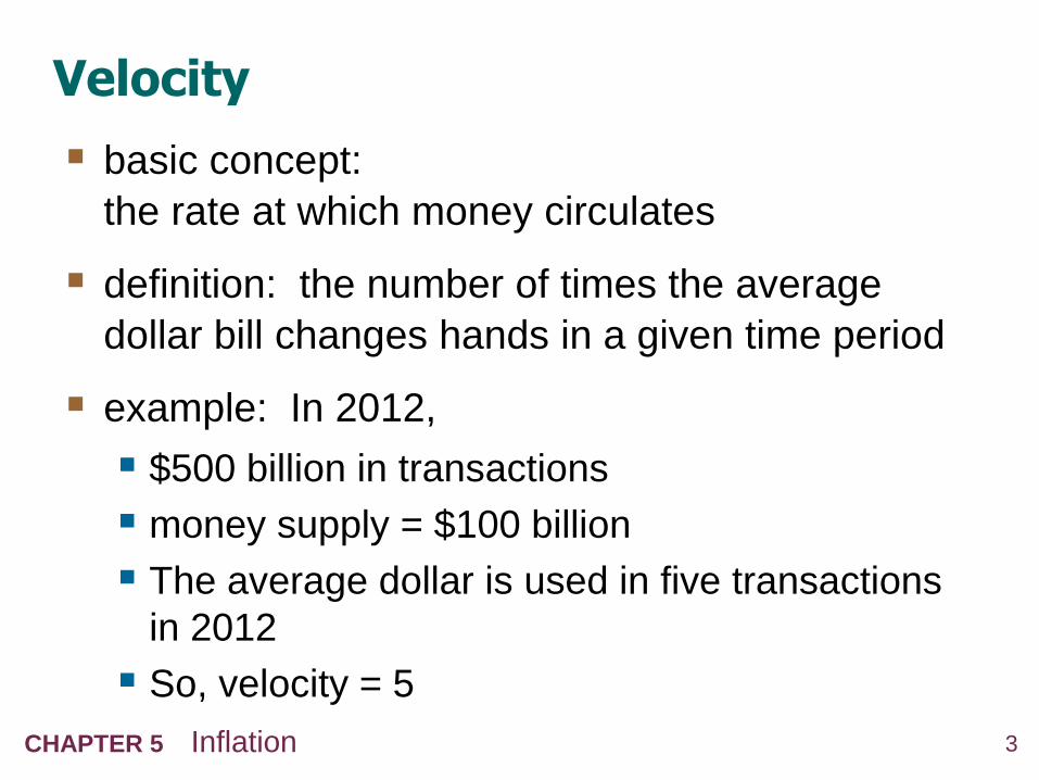
Velocity
basic concept:
the rate at which money circulates
definition: the number of times the average
dollar bill changes hands in a given time period
example: In 2012,
$500 billion in transactions
money supply = $100 billion
The average dollar is used in five transactions
in 2012
So, velocity = 5
4 CHAPTER 5 Inflation
Velocity, cont.
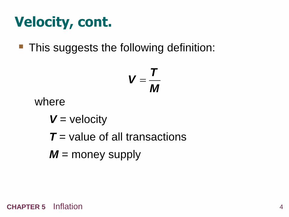
This suggests the following definition:
TV
M
where
V = velocity
T = value of all transactions
M = money supply
5 CHAPTER 5 Inflation
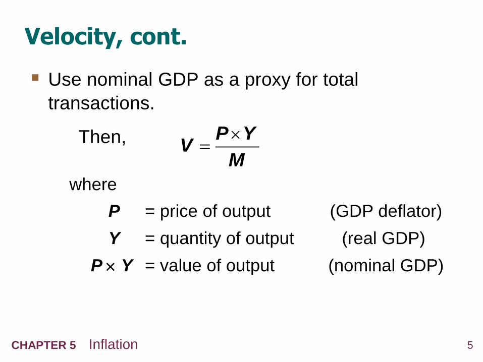
Velocity, cont.
Use nominal GDP as a proxy for total
transactions.
Then, P YV
M
where
P = price of output (GDP deflator)
Y = quantity of output (real GDP)
P Y = value of output (nominal GDP)
6 CHAPTER 5 Inflation
The quantity equation
The quantity equation
M V = P Y
follows from the preceding definition of velocity.
It is an identity:
it holds by definition of the variables.
7 CHAPTER 5 Inflation
Money demand and the quantity
equation
M/P = real money balances, the purchasing
power of the money supply.
A simple money demand function:
(M/P )d = k Y
where
k = how much money people wish to hold for
each dollar of income.
(k is exogenous)
8 CHAPTER 5 Inflation
Money demand and the quantity
equation
money demand: (M/P )d = k Y
quantity equation: M V = P Y
The connection between them: k = 1/V
When people hold lots of money relative
to their incomes (k is large),
money changes hands infrequently (V is small).
9 CHAPTER 5 Inflation
Back to the quantity theory of money
starts with quantity equation
assumes V is constant & exogenous:
Then, quantity equation becomes:
V V
M V P Y
10 CHAPTER 5 Inflation
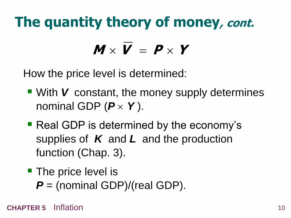
The quantity theory of money, cont.
How the price level is determined:
With V constant, the money supply determines
nominal GDP (P Y ).
Real GDP is determined by the economy’s
supplies of K and L and the production
function (Chap. 3).
The price level is
P = (nominal GDP)/(real GDP).
M V P Y
11 CHAPTER 5 Inflation
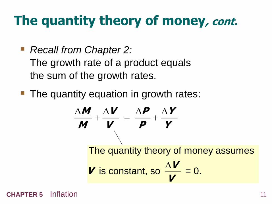
The quantity theory of money, cont.
Recall from Chapter 2:
The growth rate of a product equals
the sum of the growth rates.
The quantity equation in growth rates:
M V P Y
M V P Y
The quantity theory of money assumes
is constant, so = 0.V
VV
12 CHAPTER 5 Inflation
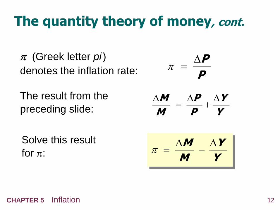
The quantity theory of money, cont.
(Greek letter pi )
denotes the inflation rate:
M P Y
M P Y
P
P
M Y
M Y
The result from the
preceding slide:
Solve this result
for :
13 CHAPTER 5 Inflation
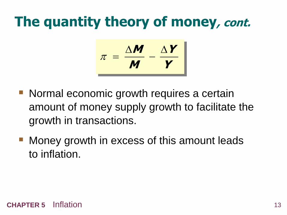
The quantity theory of money, cont.
Normal economic growth requires a certain
amount of money supply growth to facilitate the
growth in transactions.
Money growth in excess of this amount leads
to inflation.
M Y
M Y
14 CHAPTER 5 Inflation
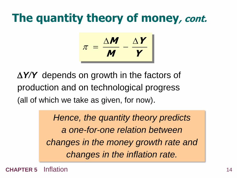
The quantity theory of money, cont.
Y/Y depends on growth in the factors of
production and on technological progress
(all of which we take as given, for now).
M Y
M Y
Hence, the quantity theory predicts
a one-for-one relation between
changes in the money growth rate and
changes in the inflation rate.
15 CHAPTER 5 Inflation
Confronting the quantity theory with
data
The quantity theory of money implies:
1. Countries with higher money growth rates
should have higher inflation rates.
2. The long-run trend in a country’s inflation rate
should be similar to the long-run trend in the
country’s money growth rate.
Are the data consistent with these implications?
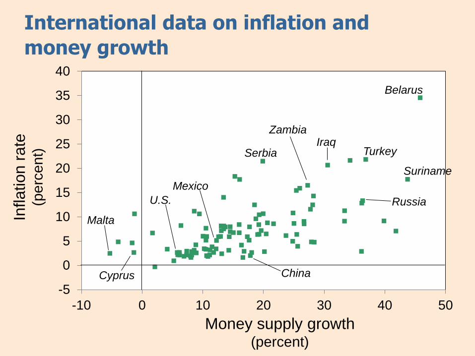
International data on inflation and
money growth
Inflation r
ate
(p
erc
ent)
Money supply growth (percent)
-5
0
5
10
15
20
25
30
35
40
-10 0 10 20 30 40 50
China
Iraq Turkey
Belarus
Zambia
U.S.
Mexico
Malta
Cyprus
Serbia
Suriname
Russia
0%
2%
4%
6%
8%
10%
12%
14%
1960 1965 1970 1975 1980 1985 1990 1995 2000 2005 2010
% c
han
ge fro
m 1
2 m
os. ea
rlie
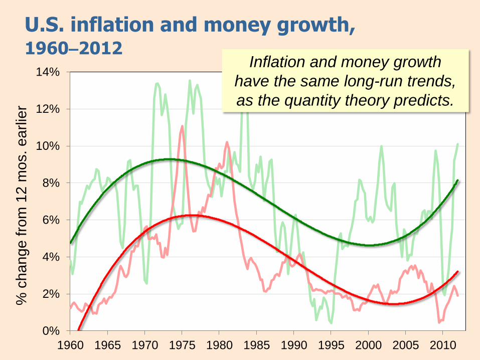
r U.S. inflation and money growth, 1960–2012
Inflation and money growth
have the same long-run trends,
as the quantity theory predicts.
18 CHAPTER 5 Inflation
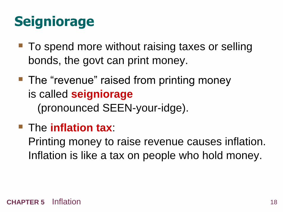
Seigniorage
To spend more without raising taxes or selling
bonds, the govt can print money.
The ―revenue‖ raised from printing money
is called seigniorage
(pronounced SEEN-your-idge).
The inflation tax:
Printing money to raise revenue causes inflation.
Inflation is like a tax on people who hold money.

19 CHAPTER 5 Inflation
Inflation and interest rates
Nominal interest rate, i
not adjusted for inflation
Real interest rate, r
adjusted for inflation:
r = i
20 CHAPTER 5 Inflation
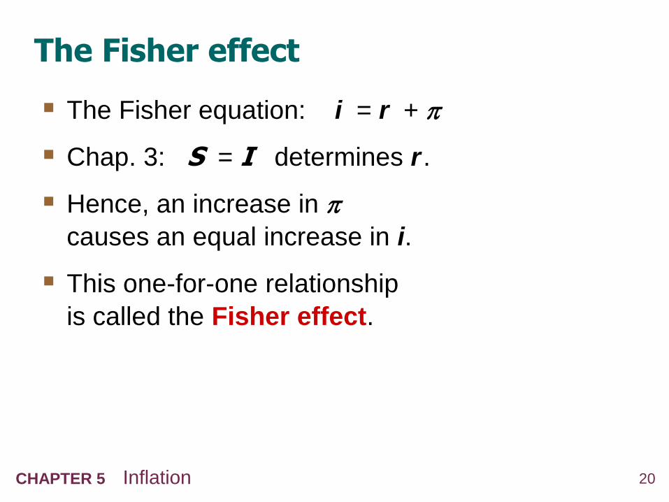
The Fisher effect
The Fisher equation: i = r +
Chap. 3: S = I determines r .
Hence, an increase in
causes an equal increase in i.
This one-for-one relationship
is called the Fisher effect.
-2%
2%
6%
10%
14%
18%
1960 1965 1970 1975 1980 1985 1990 1995 2000 2005 2010
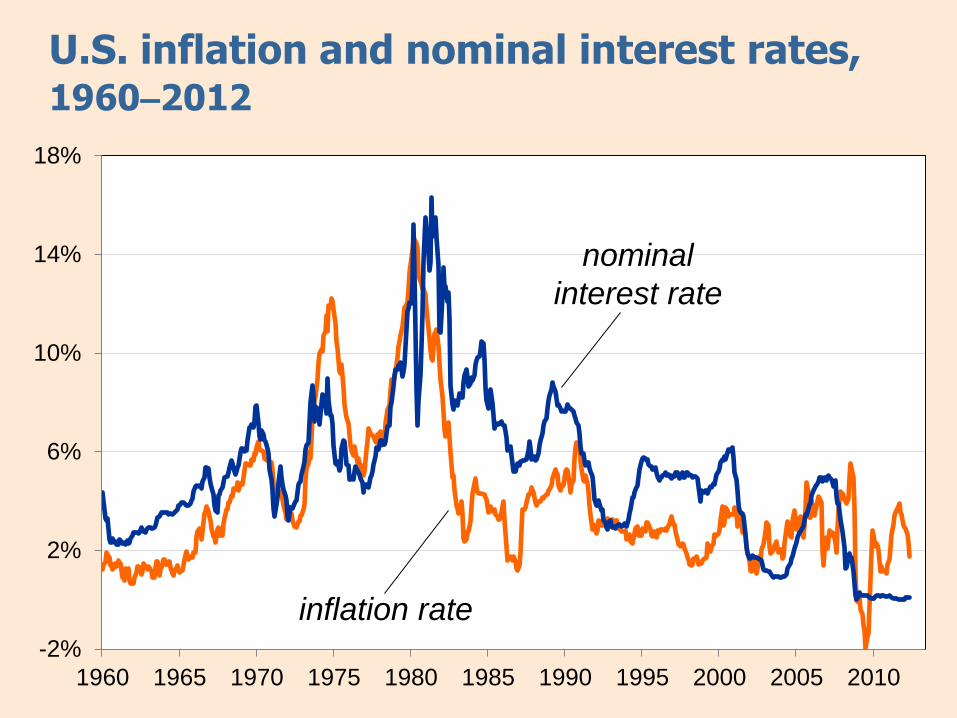
U.S. inflation and nominal interest rates, 1960–2012
inflation rate
nominal
interest rate
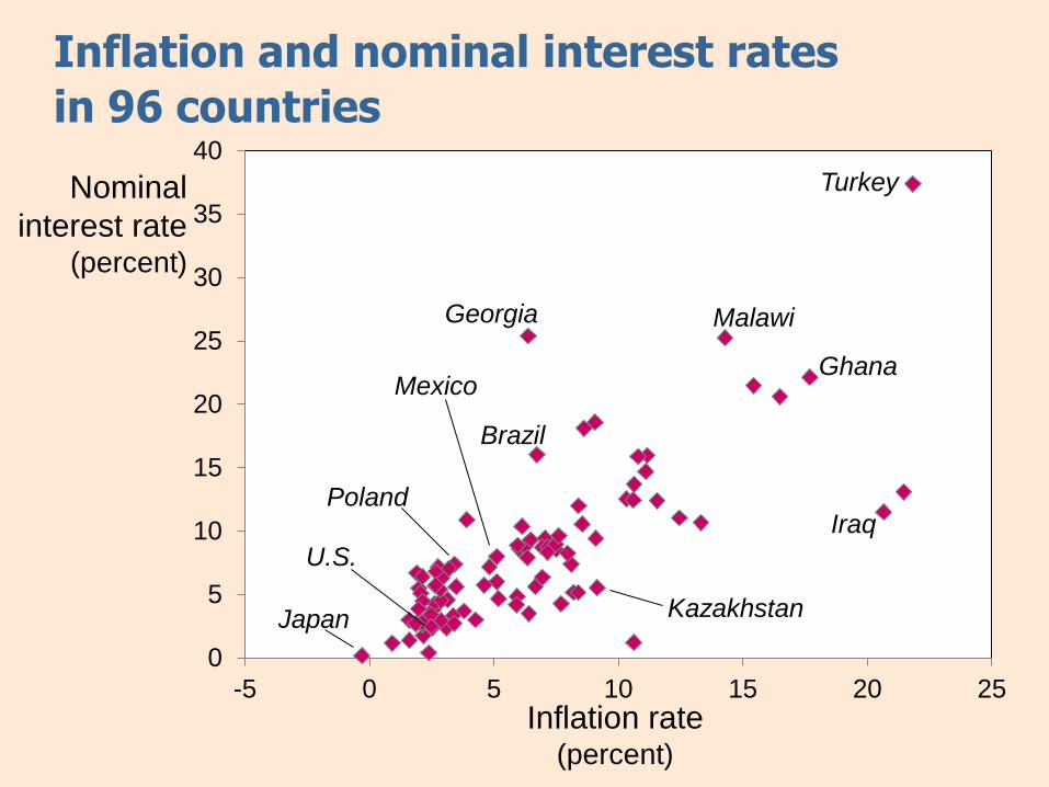
Inflation and nominal interest rates
in 96 countries
Nominal
interest rate (percent)
Inflation rate (percent)
0
5
10
15
20
25
30
35
40
-5 0 5 10 15 20 25
Malawi Georgia
Turkey
Ghana
Iraq
U.S.
Poland
Japan
Brazil
Kazakhstan
Mexico
23 CHAPTER 5 Inflation
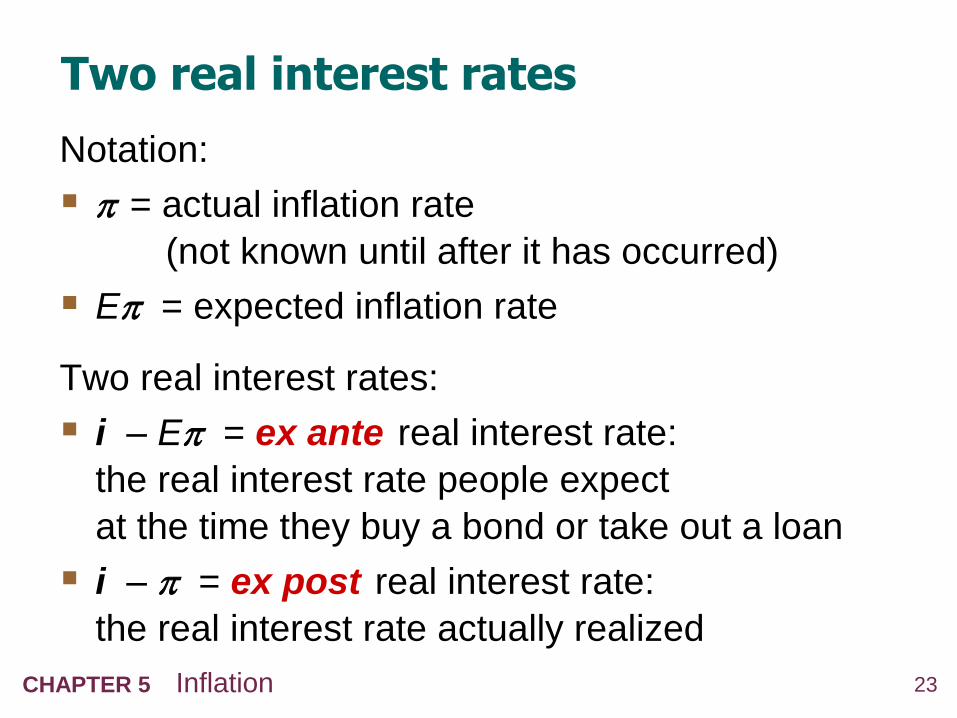
Two real interest rates
Notation:
= actual inflation rate
(not known until after it has occurred)
E = expected inflation rate
Two real interest rates:
i – E = ex ante real interest rate:
the real interest rate people expect
at the time they buy a bond or take out a loan
i – = ex post real interest rate:
the real interest rate actually realized
24 CHAPTER 5 Inflation
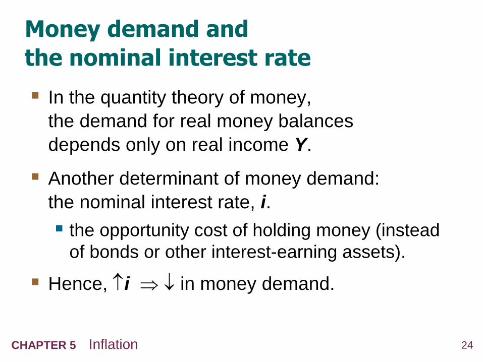
Money demand and
the nominal interest rate
In the quantity theory of money,
the demand for real money balances
depends only on real income Y.
Another determinant of money demand:
the nominal interest rate, i.
the opportunity cost of holding money (instead
of bonds or other interest-earning assets).
Hence, i in money demand.
25 CHAPTER 5 Inflation
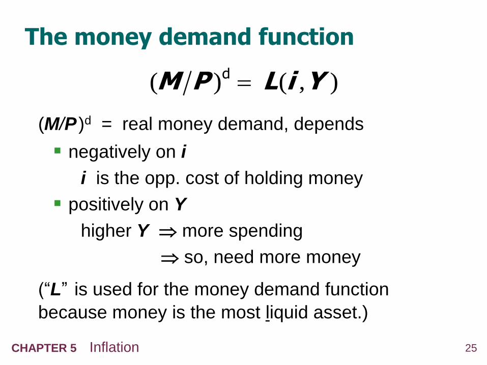
The money demand function
(M/P )d = real money demand, depends
negatively on i
i is the opp. cost of holding money
positively on Y
higher Y more spending
so, need more money
(―L‖ is used for the money demand function
because money is the most liquid asset.)
( ) ( , )dM P L i Y
26 CHAPTER 5 Inflation
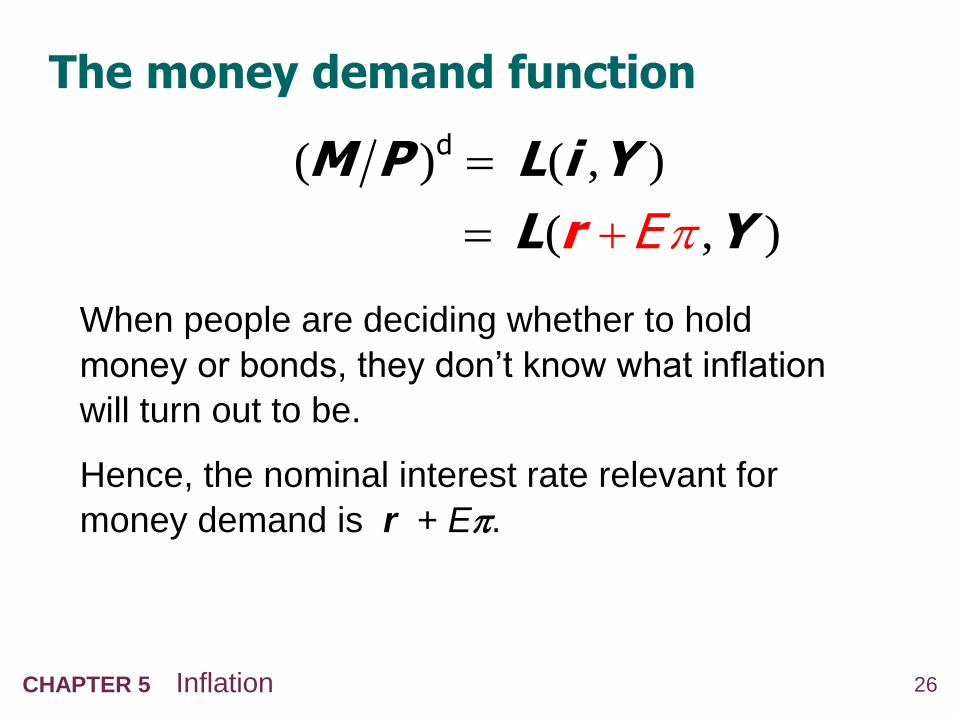
The money demand function
When people are deciding whether to hold
money or bonds, they don’t know what inflation
will turn out to be.
Hence, the nominal interest rate relevant for
money demand is r + E.
( ) ( , )dM P L i Y
( , ) rL YE
27 CHAPTER 5 Inflation
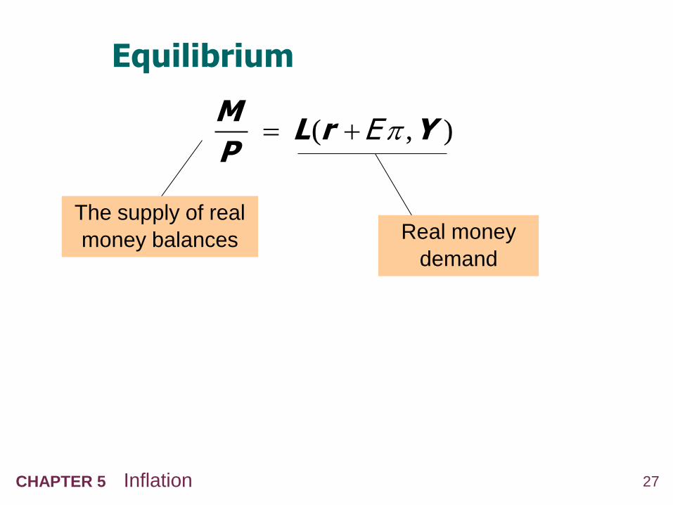
Equilibrium
( , ) M
L r YP
E
The supply of real
money balances Real money
demand

28 CHAPTER 5 Inflation
What determines what
variable how determined (in the long run)
M exogenous (the Fed)
r adjusts to ensure S = I
Y
P adjusts to ensure
( , )Y F K L
( , )M
L i YP
( , ) M
L r YP
E
29 CHAPTER 5 Inflation
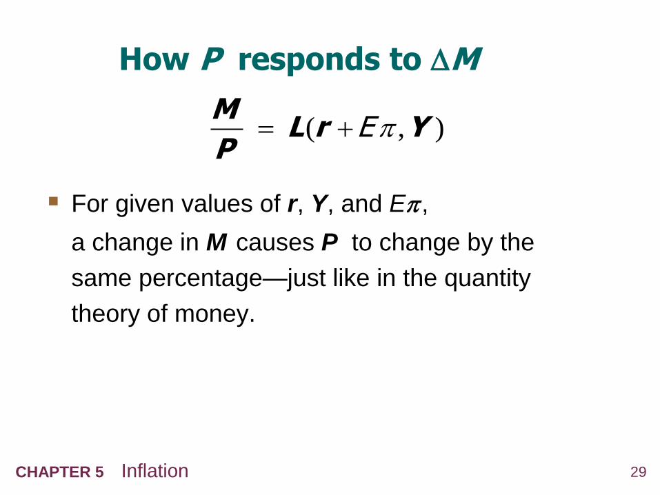
How P responds to M
For given values of r, Y, and E ,
a change in M causes P to change by the
same percentage—just like in the quantity
theory of money.
( , ) M
L r YP
E
30 CHAPTER 5 Inflation
What about expected inflation?
Over the long run, people don’t consistently
over- or under-forecast inflation,
so E = on average.
In the short run, E may change when people
get new information.
EX: Fed announces it will increase M next year.
People will expect next year’s P to be higher,
so E rises.
This affects P now, even though M hasn’t
changed yet….
31 CHAPTER 5 Inflation
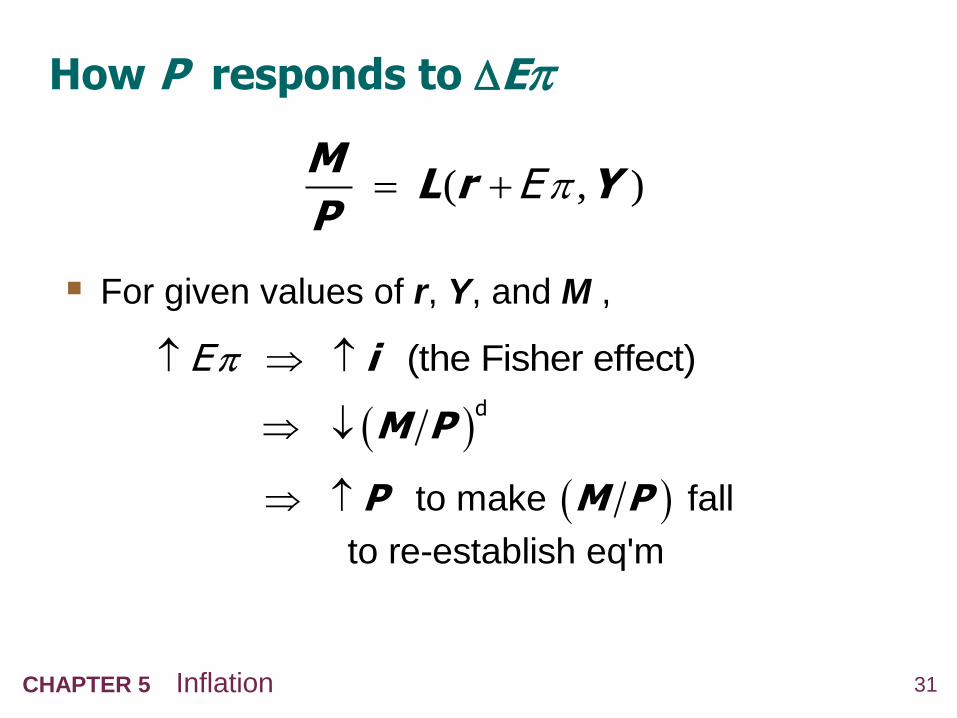
How P responds to E
(the Fisher effect)iE
d
M P
to make fall
to re-establish eq'm
P M P
For given values of r, Y, and M ,
( , ) M
L r YP
E

32 CHAPTER 5 Inflation
A common misperception
Common misperception:
inflation reduces real wages
This is true only in the short run, when nominal
wages are fixed by contracts.
(Chap. 3) In the long run,
the real wage is determined by
labor supply and the marginal product of labor,
not the price level or inflation rate.
Consider the data…
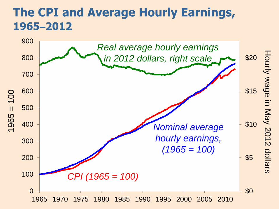
The CPI and Average Hourly Earnings, 1965–2012
19
65
= 1
00
H
ourly
wage
in M
ay 2
01
2 d
olla
rs
$0
$5
$10
$15
$20
0
100
200
300
400
500
600
700
800
900
1965 1970 1975 1980 1985 1990 1995 2000 2005 2010
Real average hourly earnings
in 2012 dollars, right scale
Nominal average
hourly earnings,
(1965 = 100)
CPI (1965 = 100)
34 CHAPTER 5 Inflation
The classical view of inflation
The classical view:
A change in the price level is merely a change
in the units of measurement.
Then, why is inflation
a social problem?
35 CHAPTER 5 Inflation
The social costs of inflation
…fall into two categories:
1. costs when inflation is expected
2. costs when inflation is different than
people had expected
36 CHAPTER 5 Inflation
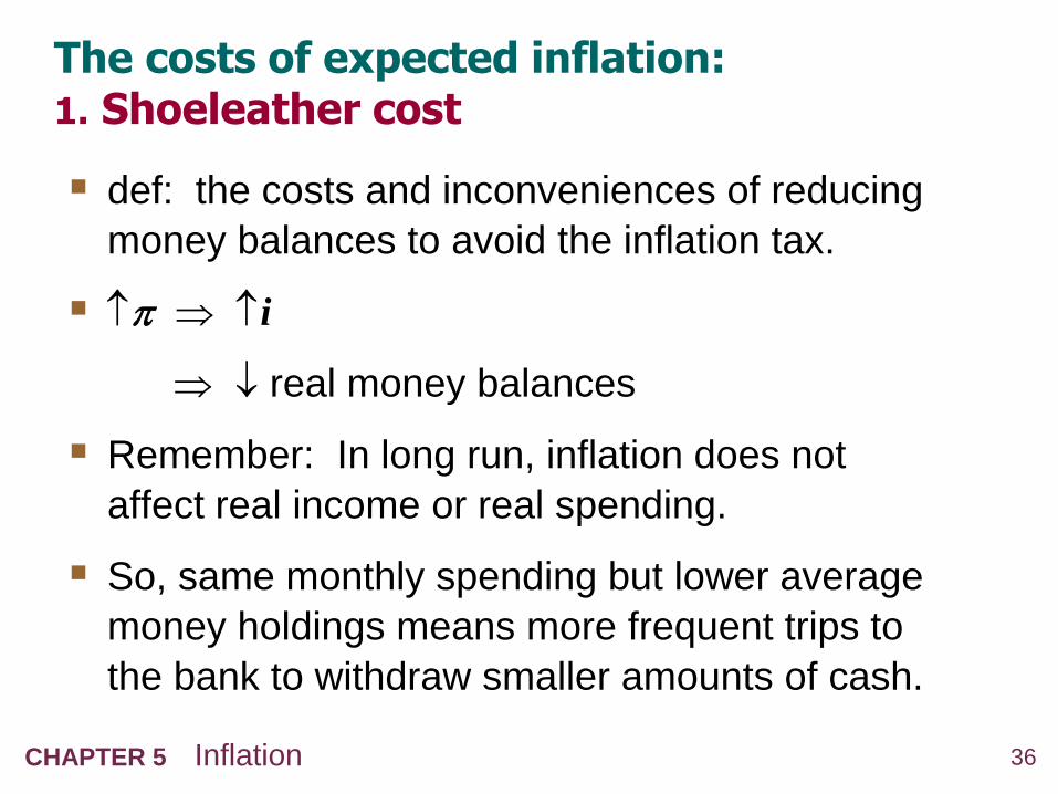
The costs of expected inflation: 1. Shoeleather cost
def: the costs and inconveniences of reducing
money balances to avoid the inflation tax.
i
real money balances
Remember: In long run, inflation does not
affect real income or real spending.
So, same monthly spending but lower average
money holdings means more frequent trips to
the bank to withdraw smaller amounts of cash.
37 CHAPTER 5 Inflation
The costs of expected inflation: 2. Menu costs
def: The costs of changing prices.
Examples:
cost of printing new menus
cost of printing & mailing new catalogs
The higher is inflation, the more frequently
firms must change their prices and incur
these costs.
38 CHAPTER 5 Inflation
The costs of expected inflation: 3. Relative price distortions
Firms facing menu costs change prices infrequently.
Example:
A firm issues new catalog each January.
As the general price level rises throughout the year,
the firm’s relative price will fall.
Different firms change their prices at different times,
leading to relative price distortions…
…causing microeconomic inefficiencies
in the allocation of resources.
39 CHAPTER 5 Inflation
The costs of expected inflation: 4. Unfair tax treatment
Some taxes are not adjusted to account for
inflation, such as the capital gains tax.
5. General inconvenience
Inflation complicates long-range financial
planning.
40 CHAPTER 5 Inflation
Additional cost of unexpected inflation: Arbitrary redistribution of purchasing power
Many long-term contracts not indexed,
but based on E .
If turns out different from E ,
then some gain at others’ expense.
Example: borrowers & lenders
If > E , then (i ) < (i E )
and purchasing power is transferred from
lenders to borrowers.
If < E , then purchasing power is
transferred from borrowers to lenders.
41 CHAPTER 5 Inflation
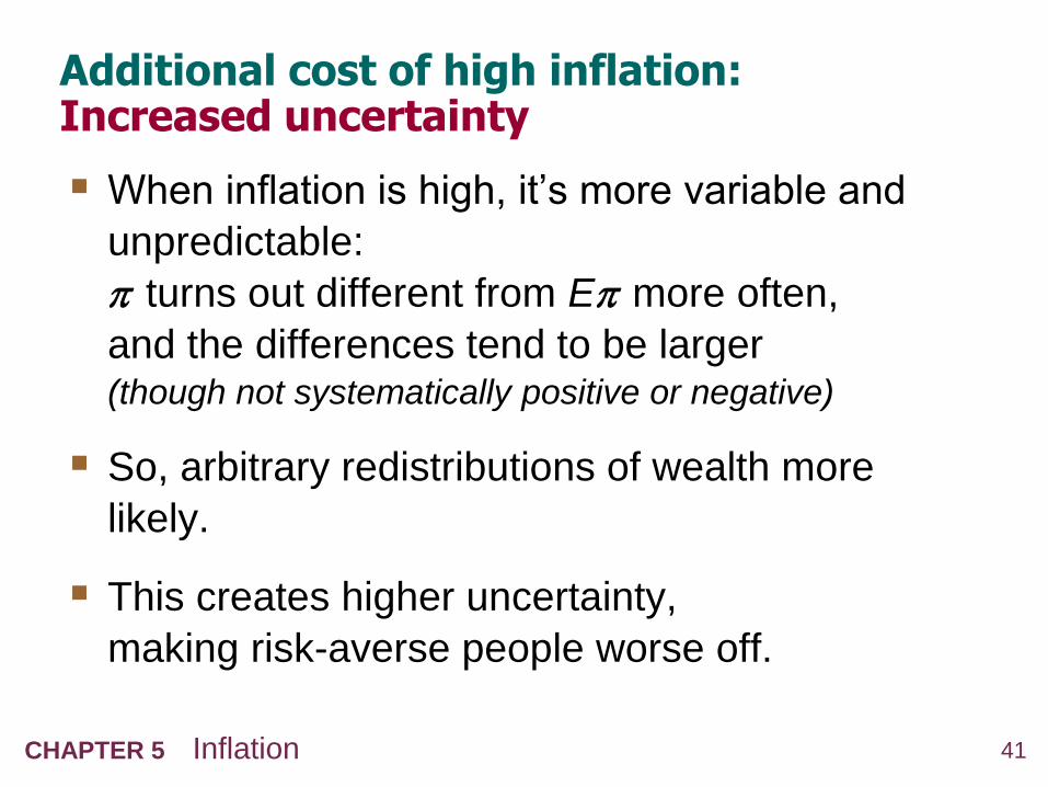
Additional cost of high inflation: Increased uncertainty
When inflation is high, it’s more variable and
unpredictable:
turns out different from E more often,
and the differences tend to be larger (though not systematically positive or negative)
So, arbitrary redistributions of wealth more
likely.
This creates higher uncertainty,
making risk-averse people worse off.
42 CHAPTER 5 Inflation
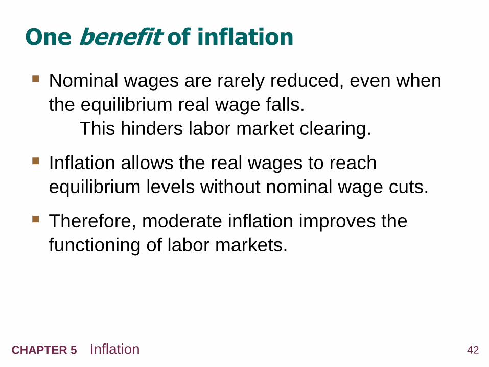
One benefit of inflation
Nominal wages are rarely reduced, even when
the equilibrium real wage falls.
This hinders labor market clearing.
Inflation allows the real wages to reach
equilibrium levels without nominal wage cuts.
Therefore, moderate inflation improves the
functioning of labor markets.
43 CHAPTER 5 Inflation
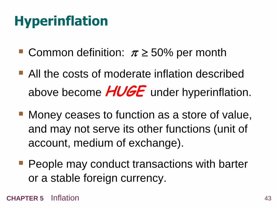
Hyperinflation
Common definition: 50% per month
All the costs of moderate inflation described
above become HUGE under hyperinflation.
Money ceases to function as a store of value,
and may not serve its other functions (unit of
account, medium of exchange).
People may conduct transactions with barter
or a stable foreign currency.
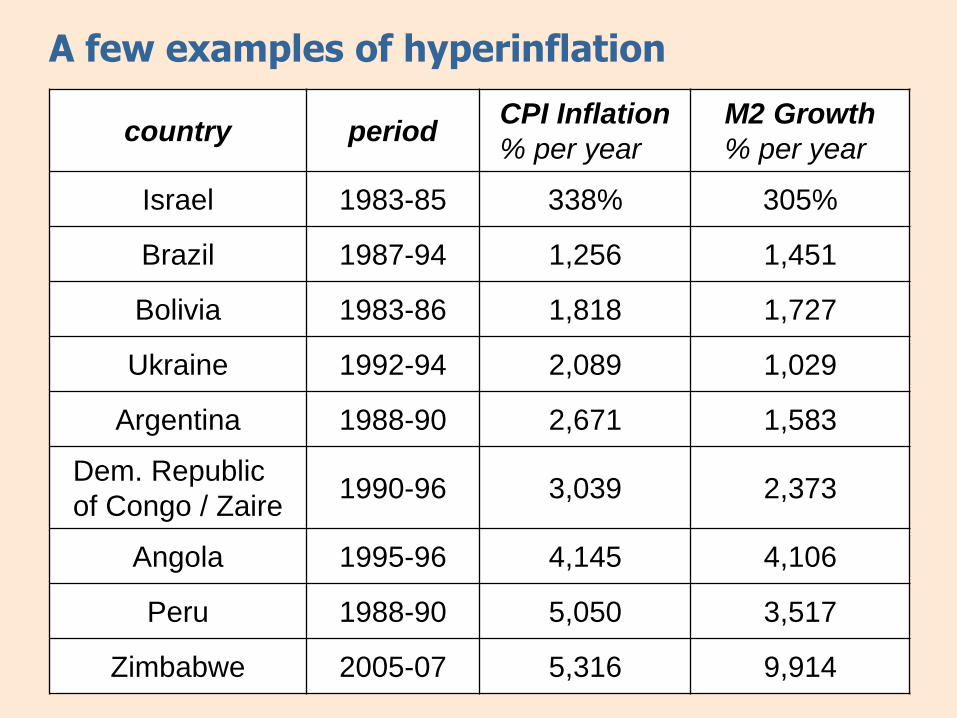
A few examples of hyperinflation
country period CPI Inflation
% per year
M2 Growth
% per year
Israel 1983-85 338% 305%
Brazil 1987-94 1,256 1,451
Bolivia 1983-86 1,818 1,727
Ukraine 1992-94 2,089 1,029
Argentina 1988-90 2,671 1,583
Dem. Republic
of Congo / Zaire 1990-96 3,039 2,373
Angola 1995-96 4,145 4,106
Peru 1988-90 5,050 3,517
Zimbabwe 2005-07 5,316 9,914

45 CHAPTER 5 Inflation
The Classical Dichotomy Real variables: Measured in physical units –
quantities and relative prices, for example:
quantity of output produced
real wage: output earned per hour of work
real interest rate: output earned in the future
by lending one unit of output today
Nominal variables: Measured in money units, e.g.,
nominal wage: Dollars per hour of work.
nominal interest rate: Dollars earned in future
by lending one dollar today.
the price level: The amount of dollars needed
to buy a representative basket of goods.
46 CHAPTER 5 Inflation
The Classical Dichotomy
Note: Real variables were explained in Chap. 3,
nominal ones in Chap. 5.
Classical dichotomy:
the theoretical separation of real and nominal
variables in the classical model, which implies
nominal variables do not affect real variables.
Neutrality of money: Changes in the money
supply do not affect real variables.
In the real world, money is approximately neutral
in the long run.