ECON 312/302: MICROECONOMICS II Lecture 7: W/C 14th …Factor Market Demand • A factor market...
37
ECON 312/302: MICROECONOMICS II Lecture 7: W/C 14 th March 2016 FACTOR MARKETS 2 Dr Ebo Turkson
Transcript of ECON 312/302: MICROECONOMICS II Lecture 7: W/C 14th …Factor Market Demand • A factor market...

ECON 312/302: MICROECONOMICS II
Lecture 7: W/C 14th March 2016
FACTOR MARKETS 2
Dr Ebo Turkson

15 - 2 Copyright © 2012 Pearson Education. All rights reserved.
Topics
• Competitive Factor Market.
Competitive factor and output markets
• Effect of Monopolies on Factor Markets.
Competitive factor and monopolized output
markets
Monopolized factor and Competitive output
markets
Monopolist in successive markets
• Monopsony.
the only buyer of a good in a given market.

15 - 3 Copyright © 2012 Pearson Education. All rights reserved.
Short-Run Factor Demand of a Firm
(cont.)
• The firm maximizes its profit by hiring
workers until the marginal revenue
product of the last worker exactly equals
the marginal cost of employing that
worker, which is the wage:
MRPL = w

15 - 4 Copyright © 2012 Pearson Education. All rights reserved.
Short-Run Factor Demand of a Firm
(cont.)
• The competitive firm hires labor to the point at
which:
MRPL = p ∙ MPL = w (1)
• The wage line is the supply of labor the firm faces.
It is horizontal (infinitely elastic)
• The marginal revenue product of labor curve,
MRPL, is the firm’s demand curve for labor
Its downward sloping because although P is fixed MPL
declines as more labour is employed.

15 - 5 Copyright © 2012 Pearson Education. All rights reserved.
Long-Run Factor Demand
• In the long run, the firm may vary all of its
inputs.
The long-run labor demand curve takes account of
changes in the firm’s use of capital as the wage
rises.

15 - 6 Copyright © 2012 Pearson Education. All rights reserved.
Figure 15.3 Labor Demand of a
Thread Mill

15 - 7 Copyright © 2012 Pearson Education. All rights reserved.
Exercises
4. A firm has a Cobb-Douglas production function
given as
q=ALαKβ
a. Solve for the factor demand functions
b. If the firms’ competitive output price is p find the
wage rate
c. What is the share of the firms revenue paid to
labour and capital?
d. If α=0.6, β=0.2 and A=1 find the LR labour and
capital demand curve equations

Chapter 15
Factor Markets
Part 2

15 - 9 Copyright © 2012 Pearson Education. All rights reserved.
Factor Market Demand
• A factor market demand curve is the sum
of the factor demand curves of the various
firms that use the input.
To derive the labor market demand curve, we
first
• determine the labor demand curve for each output
market and then
• sum across output markets to obtain the factor
market demand curve.

15 - 10 Copyright © 2012 Pearson Education. All rights reserved.
The Marginal Revenue Product Approach
• As the factor’s price falls, each firm, taking
the original market price as given, uses
more of the factor to produce more output.
As the market price falls, each firm reduces
its output and hence its demand for the input.
• A fall in an input price causes less of an increase
in factor demand than would occur if the market
price remained constant

15 - 11 Copyright © 2012 Pearson Education. All rights reserved.
Figure 15.4 Firm and Market
Demand for Labor
15 - 12 Copyright © 2012 Pearson Education. All rights reserved.
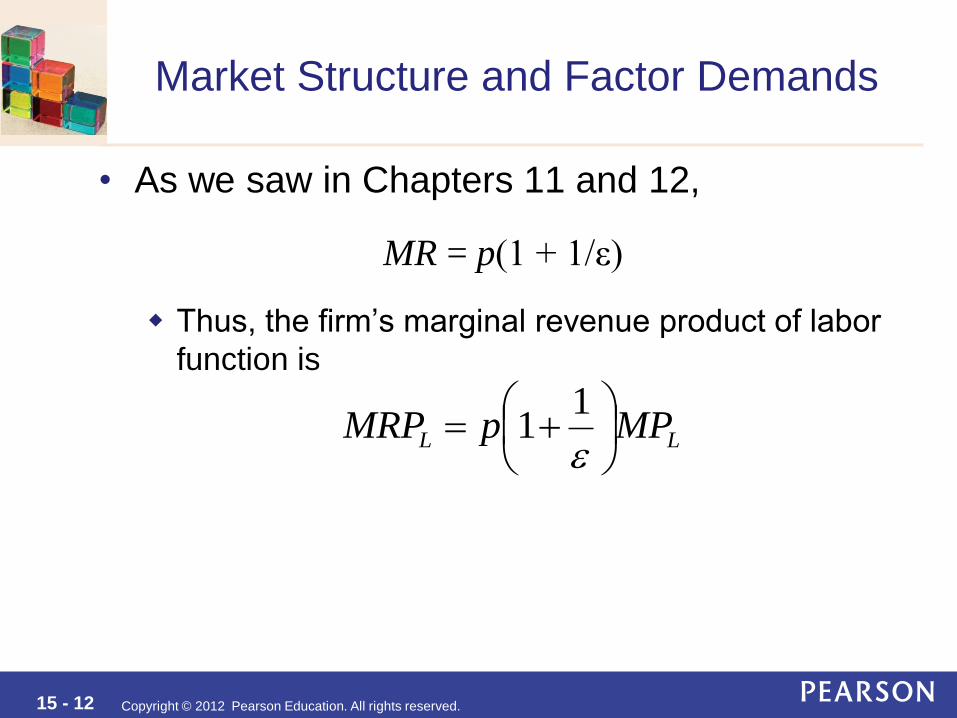
Market Structure and Factor Demands
• As we saw in Chapters 11 and 12,
MR = p(1 + 1/ε)
Thus, the firm’s marginal revenue product of labor
function is
LL MPpMRP
11

15 - 13 Copyright © 2012 Pearson Education. All rights reserved.
Figure 15.6 How Thread Mill Labor
Demand Varies with Market Structure
15 - 14 Copyright © 2012 Pearson Education. All rights reserved.
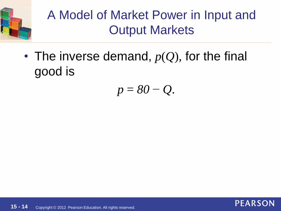
A Model of Market Power in Input and
Output Markets
• The inverse demand, p(Q), for the final
good is
p = 80 − Q.
15 - 15 Copyright © 2012 Pearson Education. All rights reserved.
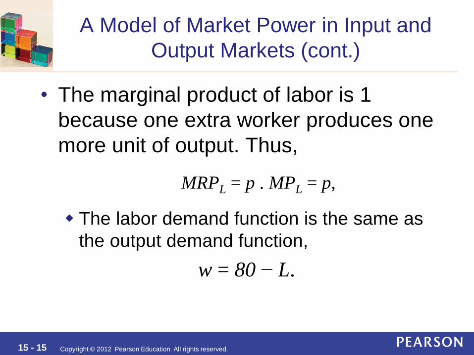
A Model of Market Power in Input and
Output Markets (cont.)
• The marginal product of labor is 1
because one extra worker produces one
more unit of output. Thus,
MRPL = p . MPL = p,
The labor demand function is the same as
the output demand function,
w = 80 − L.
15 - 16 Copyright © 2012 Pearson Education. All rights reserved.
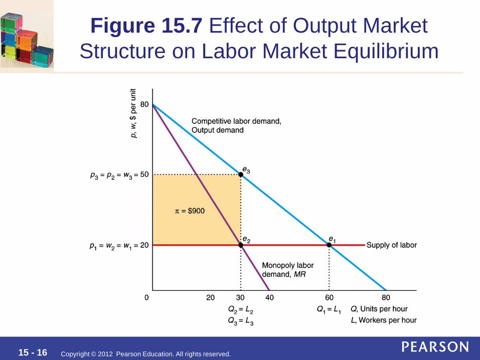
Figure 15.7 Effect of Output Market
Structure on Labor Market Equilibrium

15 - 17 Copyright © 2012 Pearson Education. All rights reserved.
Competitive Factor Market and
Monopolized Output Market
• The monopoly’s marginal revenue curve is twice as steep as the linear output demand curve it faces (Chapter 11):
MRQ = 80 − 2Q
The monopoly maximizes its profit where:
MRQ = 80 − 2Q = 20 = MC
And because the monopoly’s marginal product of labor is 1, its demand curve for labor equals its marginal revenue curve:
MRPL = MRQ × MPL = MRQ
15 - 18 Copyright © 2012 Pearson Education. All rights reserved.
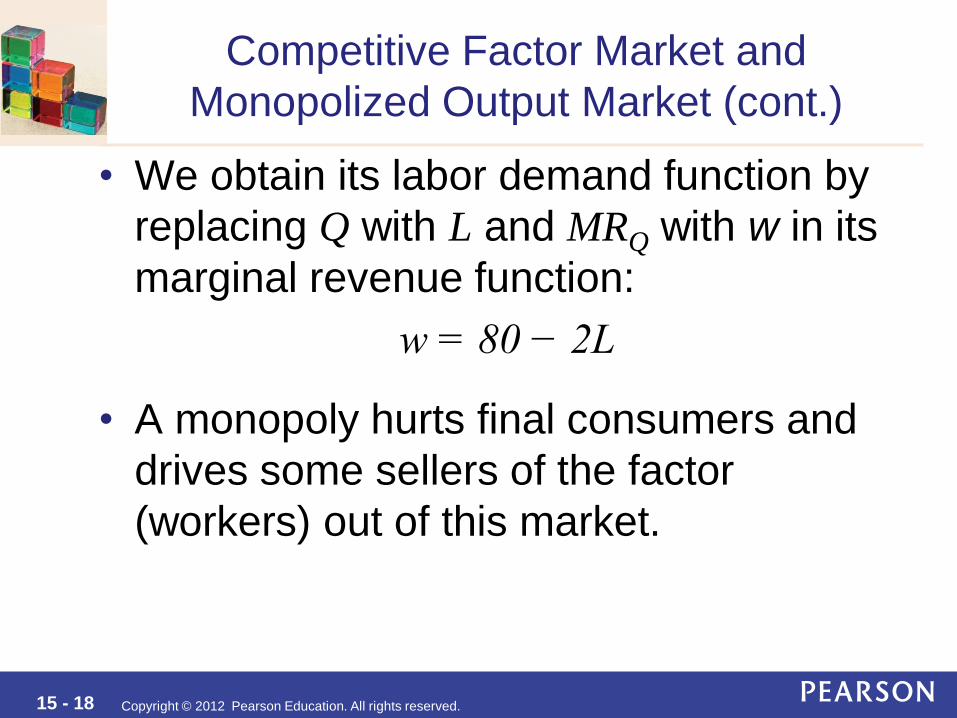
Competitive Factor Market and
Monopolized Output Market (cont.)
• We obtain its labor demand function by
replacing Q with L and MRQ with w in its
marginal revenue function:
w = 80 − 2L
• A monopoly hurts final consumers and
drives some sellers of the factor
(workers) out of this market.
15 - 19 Copyright © 2012 Pearson Education. All rights reserved.
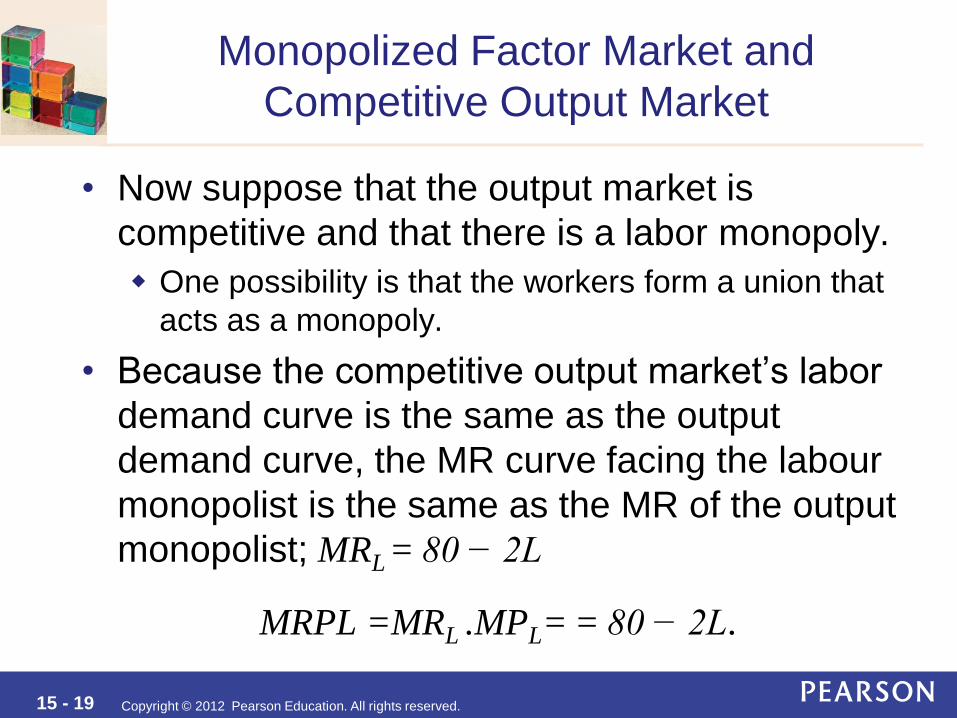
Monopolized Factor Market and
Competitive Output Market
• Now suppose that the output market is
competitive and that there is a labor monopoly.
One possibility is that the workers form a union that
acts as a monopoly.
• Because the competitive output market’s labor
demand curve is the same as the output
demand curve, the MR curve facing the labour
monopolist is the same as the MR of the output
monopolist; MRL = 80 − 2L
MRPL =MRL .MPL= = 80 − 2L.
15 - 20 Copyright © 2012 Pearson Education. All rights reserved.
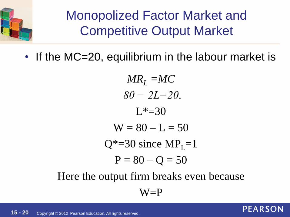
Monopolized Factor Market and
Competitive Output Market
• If the MC=20, equilibrium in the labour market is
MRL =MC
80 − 2L=20.
L*=30
W = 80 – L = 50
Q*=30 since MPL=1
P = 80 – Q = 50
Here the output firm breaks even because
W=P
15 - 21 Copyright © 2012 Pearson Education. All rights reserved.
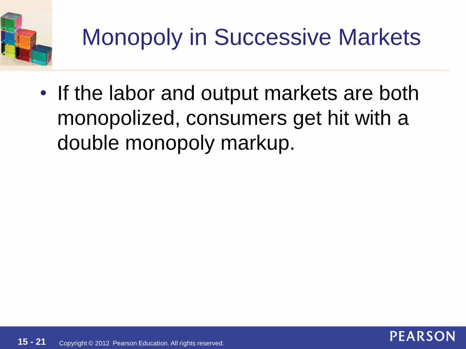
Monopoly in Successive Markets
• If the labor and output markets are both
monopolized, consumers get hit with a
double monopoly markup.
15 - 22 Copyright © 2012 Pearson Education. All rights reserved.
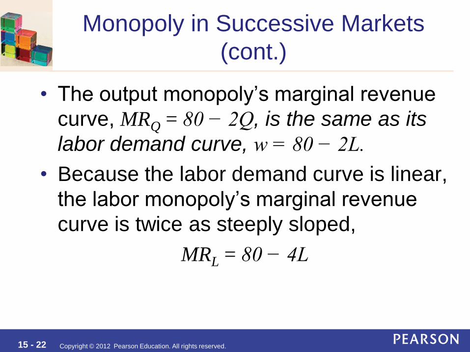
Monopoly in Successive Markets
(cont.)
• The output monopoly’s marginal revenue
curve, MRQ = 80 − 2Q, is the same as its
labor demand curve, w = 80 − 2L.
• Because the labor demand curve is linear,
the labor monopoly’s marginal revenue
curve is twice as steeply sloped,
MRL = 80 − 4L

15 - 23 Copyright © 2012 Pearson Education. All rights reserved.
Monopoly in Successive Markets
(cont.)
• If MRL = 80 − 4L
• Since MRL=MC
80 − 4L=20
L*=15
W = 80 – 2L = 50
Q*=15 since MPL=1
P = 80 – Q = 65

15 - 24 Copyright © 2012 Pearson Education. All rights reserved.
Figure 15.8 Double Monopoly Markup

15 - 25 Copyright © 2012 Pearson Education. All rights reserved.
Solved Problem 15.2
• How are consumers affected and how do
profits change in the example if the labor
monopoly buys the monopoly producer,
which is called vertical integration?

15 - 26 Copyright © 2012 Pearson Education. All rights reserved.
Monopsony
• A monopsony refers to a market condition
where there is only one buyer or
consumer. In this case one buyer of
labour input or one employer.
Here the firm in question is a sole buyer on
the input market but remains a monopolist or
PC firm on the output market
• A monopsony chooses a price-quantity
combination from the industry supply
curve that maximizes its profit.
15 - 27 Copyright © 2012 Pearson Education. All rights reserved.
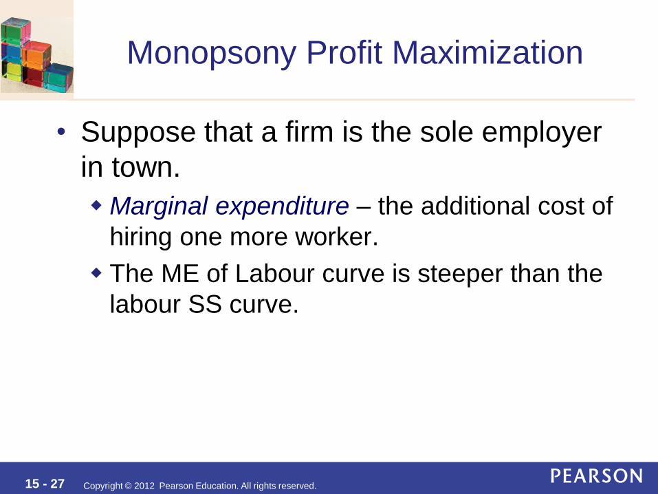
Monopsony Profit Maximization
• Suppose that a firm is the sole employer
in town.
Marginal expenditure – the additional cost of
hiring one more worker.
The ME of Labour curve is steeper than the
labour SS curve.

15 - 28 Copyright © 2012 Pearson Education. All rights reserved.
Monopsony Profit Maximization
•
15 - 29 Copyright © 2012 Pearson Education. All rights reserved.
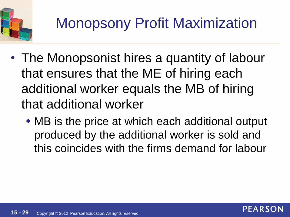
Monopsony Profit Maximization
• The Monopsonist hires a quantity of labour
that ensures that the ME of hiring each
additional worker equals the MB of hiring
that additional worker
MB is the price at which each additional output
produced by the additional worker is sold and
this coincides with the firms demand for labour

15 - 30 Copyright © 2012 Pearson Education. All rights reserved.
Monopsony Profit Maximization (cont.)
• Any buyer buys labor services up to the
point at which the marginal benefit/value
of the last unit of a factor equals the firm’s
marginal expenditure.
• Monopsony power - the ability of a single
buyer to pay less than the competitive
price profitably.

15 - 31 Copyright © 2012 Pearson Education. All rights reserved.
Figure 15.9 Monopsony and Perfect
Competitor Output Market

15 - 32 Copyright © 2012 Pearson Education. All rights reserved.
Monopsony Profit Maximization (cont.)
• The markup of the marginal expenditure
(which equals the value to the monopsony)
over the wage is inversely proportional to the
elasticity of supply at the optimum
1ME w
w

15 - 33 Copyright © 2012 Pearson Education. All rights reserved.
Monopsony and Monopolist on
Output market
W, P, ME ME
Pm=MEm A LS
P=ME B
C
W D
Wm E
LD (Same as Output Demand) =MB
Workers per day
Lm L MR

15 - 34 Copyright © 2012 Pearson Education. All rights reserved.
Welfare Effects of Monopsony
• By creating a wedge between the value to
the monopsony and the value to the
suppliers, the monopsony causes a
welfare loss in comparison to a
competitive market.

15 - 35 Copyright © 2012 Pearson Education. All rights reserved.
Figure 15.10 Welfare Effects of
Monopsony
15 - 36 Copyright © 2012 Pearson Education. All rights reserved.
Solved Problem 15.3
• How does the equilibrium in a labor
market with a monopsony employer
change if a minimum wage is set at the
competitive level?
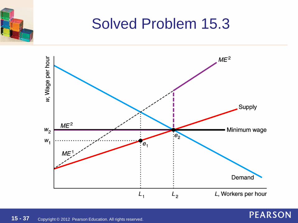
15 - 37 Copyright © 2012 Pearson Education. All rights reserved.
Solved Problem 15.3