Ecological role of the salamander Ensatina eschscholtzii: direct impacts

on the arthropod assemblage and indirect influence on the carbon cycle

in mixed hardwood/conifer forest in Northwestern California

By

Michael Best

A Thesis

Presented to

The faculty of Humboldt State University

In Partial Fulfillment

Of the Requirements for the Degree

Masters of Science

In Natural Resources: Wildlife

August 10, 2012

iii

ABSTRACT

Ecological role of the salamander Ensatina eschscholtzii: direct impacts on the arthropod

assemblage and indirect influence on the carbon cycle in mixed hardwood/conifer forest

in Northwestern California

Michael Best

Terrestrial salamanders are the most abundant vertebrate predators in

northwestern California forests, fulfilling a vital role converting invertebrate to vertebrate

biomass. The most common of these salamanders in northwestern California is the

salamander Ensatina (Ensatina eschsccholtzii). I examined the top-down effects of

Ensatina on leaf litter invertebrates, and how these effects influence the relative amount

of leaf litter retained for decomposition, thereby fostering the input of carbon and

nutrients to the forest soil. The experiment ran during the wet season (November - May)

of two years (2007-2009) in the Mattole watershed of northwest California. In Year One

results revealed a top-down effect on multiple invertebrate taxa, resulting in a 13%

difference in litter weight. The retention of more leaf litter on salamander plots was

attributed to Ensatina’s selective removal of large invertebrate shedders (beetle and fly

larva) and grazers (beetles, springtails, and earwigs), which also enabled small grazers

(mites; barklice in year two) to become more numerous. Ensatina’s predation modified

the composition of the invertebrate assemblage by shifting the densities of members of a

key functional group (shredders) resulting in an overall increase in leaf litter retention.

Results from year two indicated that these effects were affected by moisture availability,

and that direct salamander impacts on invertebrates, and the related indirect effects on the

capacity for forest floor leaf litter retention were diminished in the second, wetter year.

iv

ACKNOWLEDGMENTS

First and foremost I must thank my parents for constantly nurturing the young

scientist within me; allowing their 6 year old son to tromp around the neighborhood with

a heavy 35 mm Nikon, enabling me to capture photos of insects and habitat. I am

inspired by their endless support and now look to my two children, ripe with a sea of

discoveries, directing my constant observation of the World from a new perspective. I

am so grateful for the humbling and educational guidance only parenthood could provide.

Next I have to thank Dr. H. Welsh Jr. for bringing me through this process of

development into fruition as I (and my work) transitioned from biologist to scientist. I

now feel prepared and motivated to tackle any scientific inquiry rigorously and

effectively. His expertise and graceful nature offered a singular gracious experience.

I am forever grateful to J. Baldwin for guiding my statistical analysis and writing

the many lines of code, enabling me to capture all the results at once rather than clumsily

stumbling through it on my own. The completion of this thesis also may not have been

possible without a writing grant from the Amphibian and Reptile Conservancy. I must

also acknowledge J. Gibbs for initially turning me on to reptile and amphibian

conservation and N. Karraker for sending me out to Northern coastal California in 2005,

wetting my appetite for the study of California amphibians.

Finally, digging trenches and collecting data in the rain, by my side on cold winter

days was my loving life partner Jada. I would not be who I am today without her

support. Her unconditional bond and universal wisdom are unprecedented and have

forever opened my eyes to the true power of love and commitment. The family she has

given me will continue to enrich our lives and inspires me to be the best I can be.

v

TABLE OF CONTENTS

Page

ABSTRACT........................................................................................................................iii

ACKNOWLEDGMENTS..................................................................................................iv

LIST OF TABLES..............................................................................................................vi

LIST OF FIGURES...........................................................................................................vii

INTRODUCTION..............................................................................................................1

STUDY SITE......................................................................................................................4

MATERIALS AND METHODS........................................................................................5

Experimental design...............................................................................................5

Timing……………….............................................................................................8

Invertebrate samples…...........................................................................................8

Leaf litter bags.......................................................................................................11

Statistical analysis.................................................................................................12

RESULTS..........................................................................................................................15

Ensatina effects on invertebrate taxa.....................................................................21

Leaf-litter...............................................................................................................34

DISCUSSION....................................................................................................................36

The influence of moisture and prey density……………………………...............40

Ensatina and optimal foraging theory....................................................................41

CONCLUSIONS AND RECOMMENDATIONS.............................................................44

LITERATURE CITED.......................................................................................................45

APPENDIX A....................................................................................................................50

vi

LIST OF TABLES

Table Page

1 General linear model equation terms and their explanations; used in the

Analysis comparing invertebrate samples across plots in each year.………… 14

2 Analysis of the effects of salamander predation, moisture, month, and the

interaction of month*moisture, on invertebrate functional groups by size

class in two years using a general linear model. Data were analyzed

separately by group, size, and year. Results indicated with – were not

statistically significant at α = 0.1……………………………………………… 20

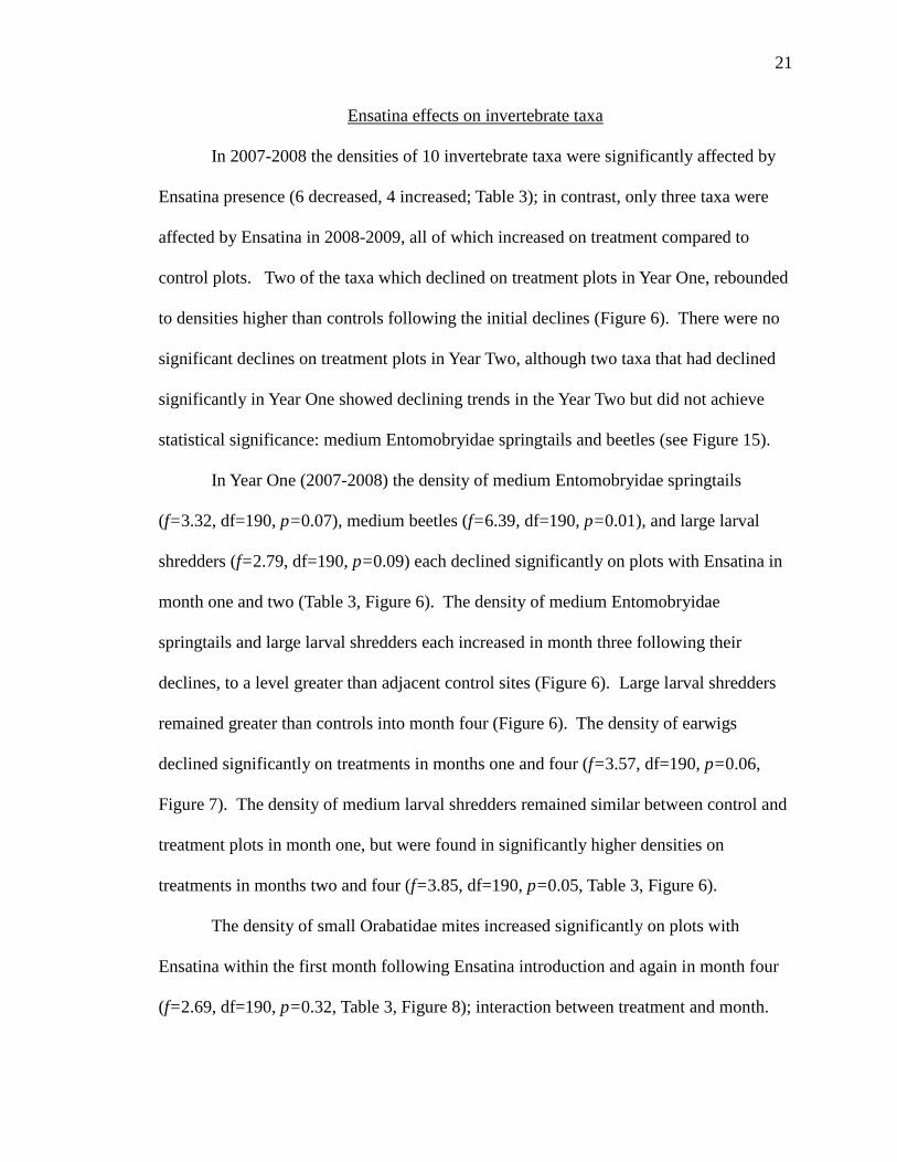
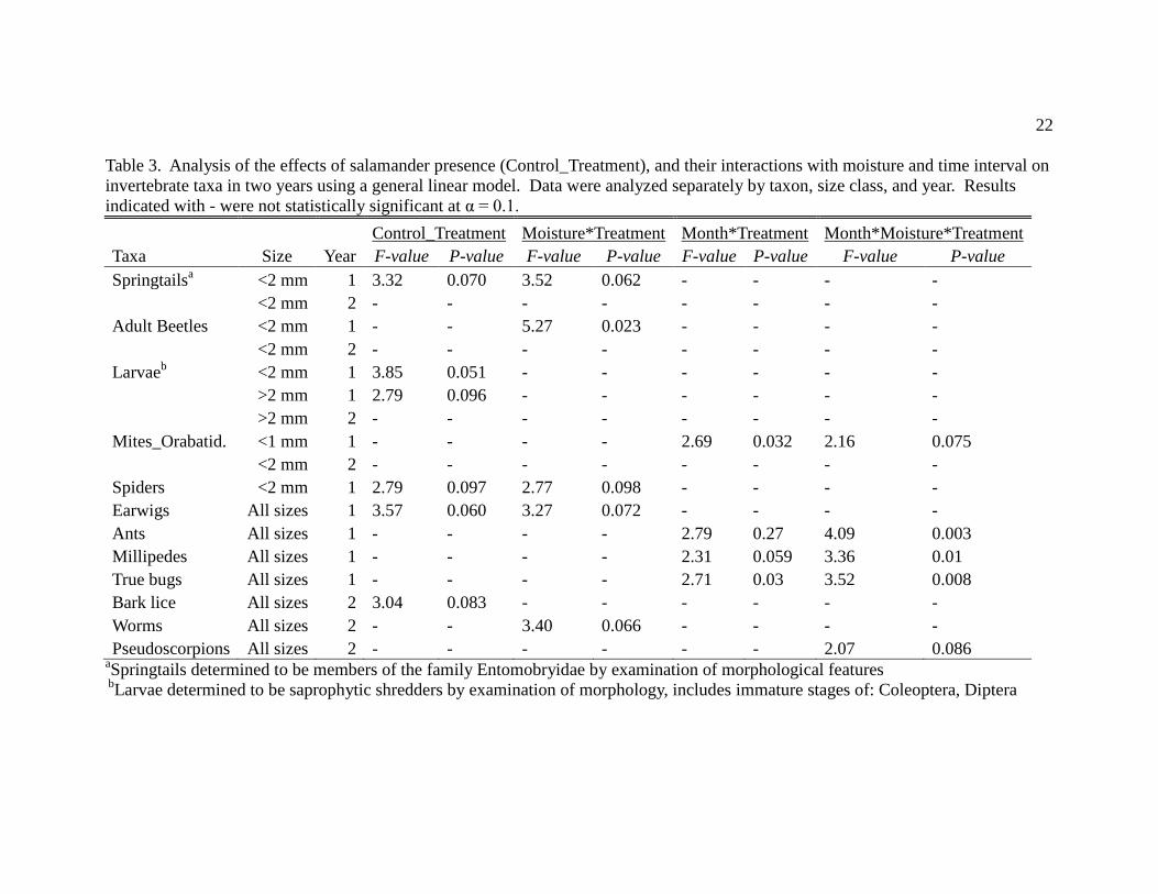
3 Analysis of the effects of salamander presence (Control_Treatment), and

their interactions with moisture and time interval on invertebrate taxa in two

years using a general linear model. Data were analyzed separately by taxon,

size class, and year. Results indicated with - were not statistically significant

at α = 0.1.……………………………………………………………………… 22

vii

LIST OF FIGURES

Figure Page

1 Experimental enclosures to assess the impacts of Ensatina on invertebrate and

litter turnover in situ at the field location near Ettersburg, California. Enclosure

dimensions were 3 m x 3 m x 23 cm, plot dimensions = 1.5 m x 1.5 m x 23 cm. 6

2 Density of invertebrates by functional group, with the two most abundant taxa

within the decomposers, mites and springtails represented separately.

Invertebrates were extracted from litter samples collected within experimental

plots near Ettersburg, California in 2007-2008. Values above bars are relative

composition out of all invertebrates found represented as percentage of 100…. 16

3 Density of invertebrates by functional group, with the two most abundant taxa

within the decomposers, mites and springtails represented separately.

Invertebrates were extracted from litter samples collected within experimental

plots near Ettersburg, California in 2008-2009. Values above bars are relative

composition out of all invertebrates found represented as percentage of 100…. 17

4 Mean density of: invertebrates and invertebrate decomposers <1mm on control

and treatment plots sampled at 5 monthly intervals in 2007-2008 from Mattole

field sites near Ettersburg, California. The blue line represents the percent litter

moisture in 2007-2008. Error bars are ± one standard error…………………... 18

5 Mean density of: invertebrates and invertebrate decomposers <1mm on control

and treatment plots sampled at 5 monthly intervals in 2008-2009 from Mattole

field sites near Ettersburg, California. The blue line represents the percent litter

moisture in 2008-2009. Error bars are ± one standard error….......................... 19

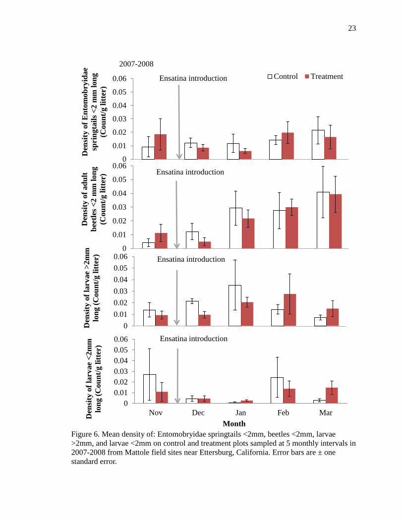
6 Mean density of: Entomobryidae springtails <2mm, beetles <2mm, larvae

>2mm, and larvae <2mm on control and treatment plots sampled at 5 monthly

intervals in 2007-2008 from Mattole field sites near Ettersburg, California.

Error bars are ± one standard error………..……………………………………. 23

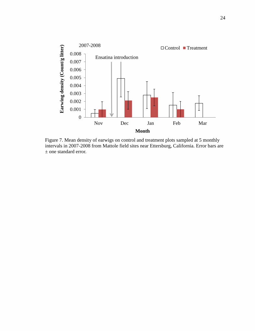
7 Mean density of earwigs on control and treatment plots sampled at 5 monthly

intervals in 2007-2008 from Mattole field sites near Ettersburg, California.

Error bars are ± one standard error……………………………………………... 24

8 Mean density of Orabatidae mites <1mm on control and treatment plots

sampled at 5 monthly intervals in 2007-2008 from Mattole field sites near

Ettersburg, California. Error bars are ± one standard error…………………… 25

viii

LIST OF FIGURES (CONTINUED)

Figure Page

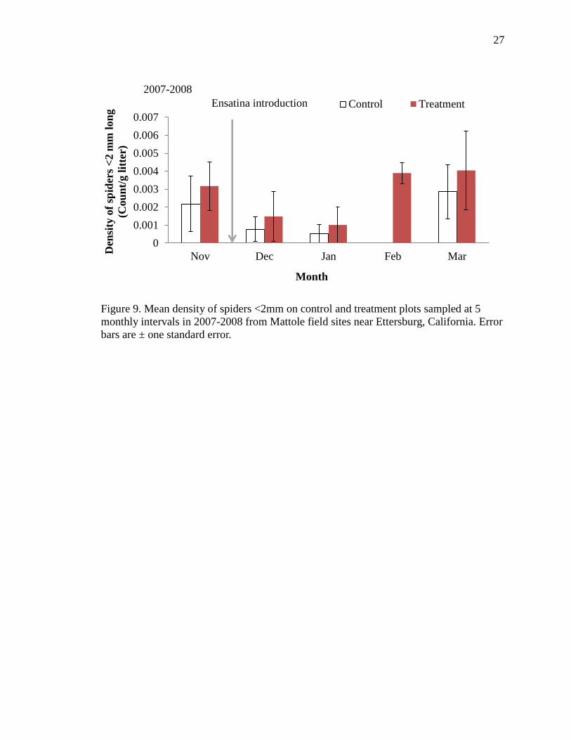
9 Mean density of spiders <2mm on control and treatment plots sampled at 5

monthly intervals in 2007-2008 from Mattole field sites near Ettersburg,

California. Error bars are ± one standard error………………………………… 27

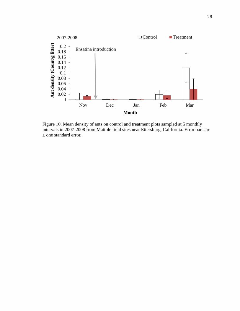
10 Mean density of ants on control and treatment plots sampled at 5 monthly

intervals in 2007-2008 from Mattole field sites near Ettersburg, California.

Error bars are ± one standard error…………………………………………….. 28

11 Mean density of millipedes on control and treatment plots sampled at 5

monthly intervals in 2007-2008 from Mattole field sites near Ettersburg,

California. Error bars are ± one standard error……………………………….. 29

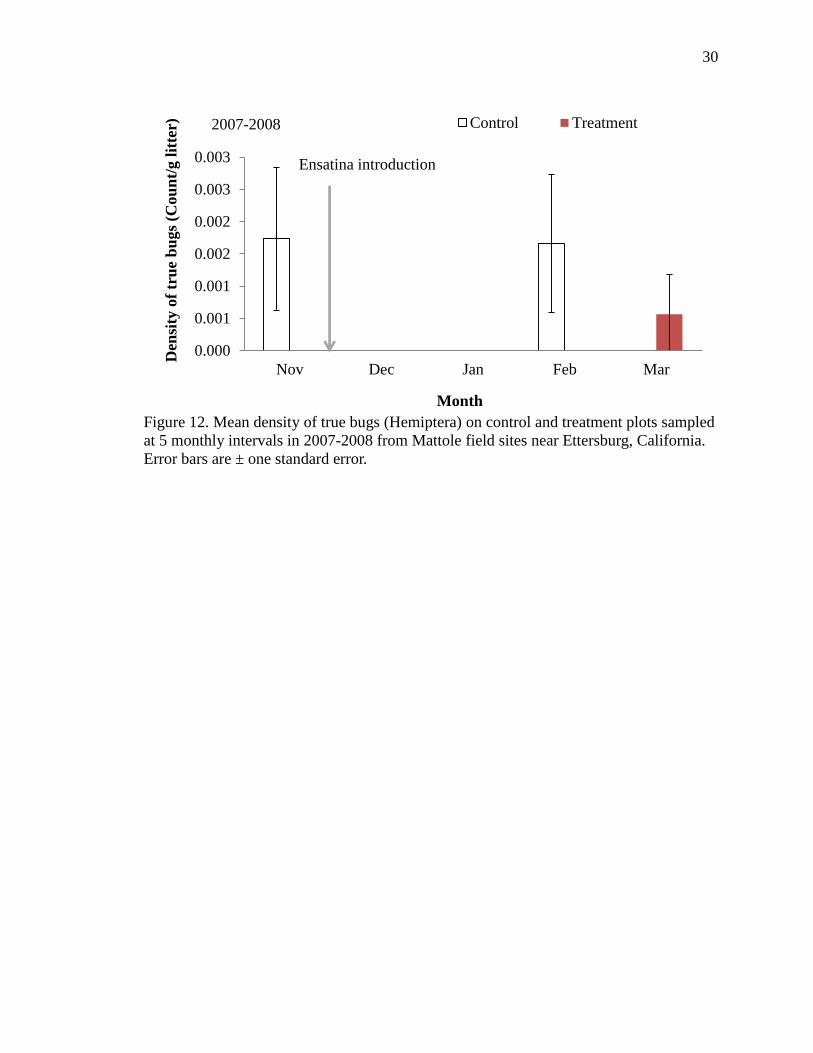
12 Mean density of true bugs (Hemiptera) on control and treatment plots sampled

at 5 monthly intervals in 2007-2008 from Mattole field sites near Ettersburg,

California. Error bars are ± one standard error……………………………….. 30

13 Mean density of: barklice (Psocoptera) and worms (Annelida) on control and

treatment plots sampled at 5 monthly intervals in 2008-2009 from Mattole

field sites near Ettersburg, California. Error bars are ± one standard error…... 31

14 Mean density of Pseudoscorpions on control and treatment plots sampled at 5

monthly intervals in 2008-2009 from Mattole field sites near Ettersburg,

California. Error bars are ± one standard error.…………………….…………. 32

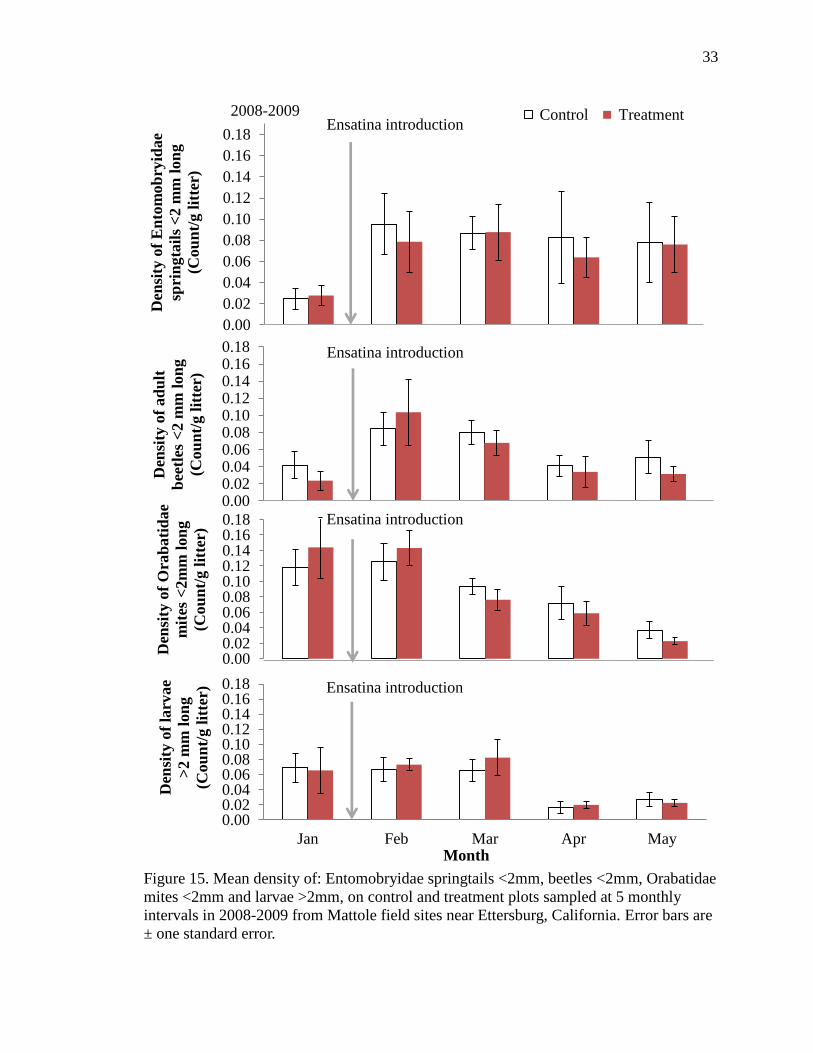
15 Mean density of: Entomobryidae springtails <2mm, beetles <2mm,

Orabatidae mites <2mm and larvae >2mm on control and treatment plots

sampled at 5 monthly intervals in 2008-2009 from Mattole field sites near

Ettersburg, California. Error bars are ± one standard error................................ 33

16 Mean leaf litter weight (g) on treatment and control plots in: Year One (2007-

2008); and Year Two (2008-2009), at the Mattole field sites near Ettersburg,

California. Error bars are ± one standard deviation.…………………………. 35

1

INTRODUCTION

Woodland (plethodontid) salamanders are the most abundant vertebrate predators

in northwestern California forests (Welsh and Lind 1991), where based on their numbers

and biomass they are ecologically dominant, filling a key nutrient cycling role:

converting invertebrate to vertebrate biomass (Burton and Likens 1975a). Burton and

Likens (1975b) found one species of plethodontid salamander (Plethodon cinereus) in an

eastern U.S. hardwood forest comprised greater biomass than all the songbirds and equal

to that of all the small mammals combined. At a North Carolina forest site Petranka and

Murray (2001) reported the entire plethodontid assemblage comprised six times the

number of individuals and 14 times the biomass reported by Burton and Likens (1975b).

Welsh and Lind (1992) reported an extremely high density for a single species of

plethodontid salamander at a mixed conifer/hardwood forest site in northern California.

In a New York forest, Wyman (1998) found that the consumption of invertebrates by the

most abundant plethodontid salamander Plethodon cinereus increased forest floor carbon

retention by reducing leaf-litter breakdown 11-17%. Walton (2005) found that this

process was not straight-forward, and might be affected by variability in both leaf litter

mass and moisture content. Results from other studies have provided evidence that

invertebrate densities might have increased in the presence of terrestrial salamanders

(Rooney 2000, Walton et al. 2006) or have had negligible effects on invertebrates

(Homyack et al. 2010), however, having no significant effect on leaf litter breakdown.

Complex food webs can be regulated both from below, where abiotic factors (e.g.,

nutrients, moisture, etc.) control the potential for productivity (bottom-up effects), and

2

simultaneously from above by predation, disease, parasitism, etc. (top-down effects) (e.g.,

Benrong and Wise 1999, Gruner 2004, Bridgeland et al. 2010). The bottom-up effects

can both promote or restrict the higher trophic levels from below, while predation or its

absence can similarly influence the system from above (McCay and Storm 1997,

Benrong and Wise 1999, Kagata and Ohgushi 2006).

Wyman (1998) found all invertebrate groups he sampled were reduced by

salamanders in field enclosures, while other studies using both lab and field enclosures

found Podomorphic springtails (Collembola) increased while other invertebrate taxa

decreased, in the presence of salamanders (Rooney 2000, Walton and Steckler 2005,

Walton et al. 2006). Walton and Steckler (2005) attributed the increase in Podomorphic

springtails to selection by salamanders for larger prey, releasing smaller arthropods from

competition and depredation by invertebrate predators, along with the effect of enhancing

their microfloral food base via salamander feces deposition. In contrast, avoiding the use

of enclosures, Walton (2005) found no significant top-down effects from salamanders

over the first year and instead found moisture and litter mass influenced invertebrate

densities. However, in the following year, salamander presence was the single significant

factor that influenced invertebrate densities in the spring; the combination of salamanders

and litter mass significantly influenced invertebrate densities in the fall (Walton 2005).

The Ensatina salamander (Ensatina eschscholtzii; hereafter Ensatina), a member

of the family Plethodontidae, is the most abundant terrestrial salamander in the mixed

hardwood/ Douglas-fir forests of Northwestern California (Welsh and Lind 1991).

Terrestrial salamanders feed on most arthropods including springtails, mites, and beetles

(Bury and Martin 1973, Lynch 1985, Rooney 2000). Many small arthropods are

3

important decomposers of forest leaf litter, an assemblage dominated by mites and

springtails (Gist and Crossley 1975, Singh 1977). An analysis of stomach content of

Ensatina and another common plethodontid species, the California slender salamander

(Batrachoseps attenuatus), in redwood forest (Sequoia sempervirens) found springtails

were the most common prey consumed, followed by mites, which were equal in number

to springtails in the slender salamander (Bury and Martin 1973). The importance of

small invertebrate decomposers in the diets of these abundant salamanders indicates the

ecologically dominant influence they can have on the capacity of the forest litter layer to

sequester or release carbon and cycle important nutrients at the litter-soil interface (Gist

and Crossley 1975, Singh 1977).

Studies of the roles of terrestrial salamanders in forest detrital food web dynamics

have not been conducted in the Western United States. The objective of my study was to

determine how Ensatina predation impacted the densities of members of the forest

invertebrate assemblage, and how this may have affected the breakdown of leaf-litter;

which indirectly influenced the relative amount of carbon and nutrients retained at the

litter/soil interface in mixed hardwood-conifer forests in Northwestern California.

I evaluated the following hypotheses in a mixed hardwood/conifer forest of

northern California: (1) Ensatina had a top down influence via predation on the

composition and densities of invertebrates dwelling in the forest floor litter; (2) leaf litter

breakdown in this forest floor food web was reduced via this predation on plots with

Ensatina compared to controls; and (3) available moisture affected these dynamics by

influencing the relative abundances of the invertebrates and the rate of litter breakdown

in this leaf litter food web.

4

STUDY SITE

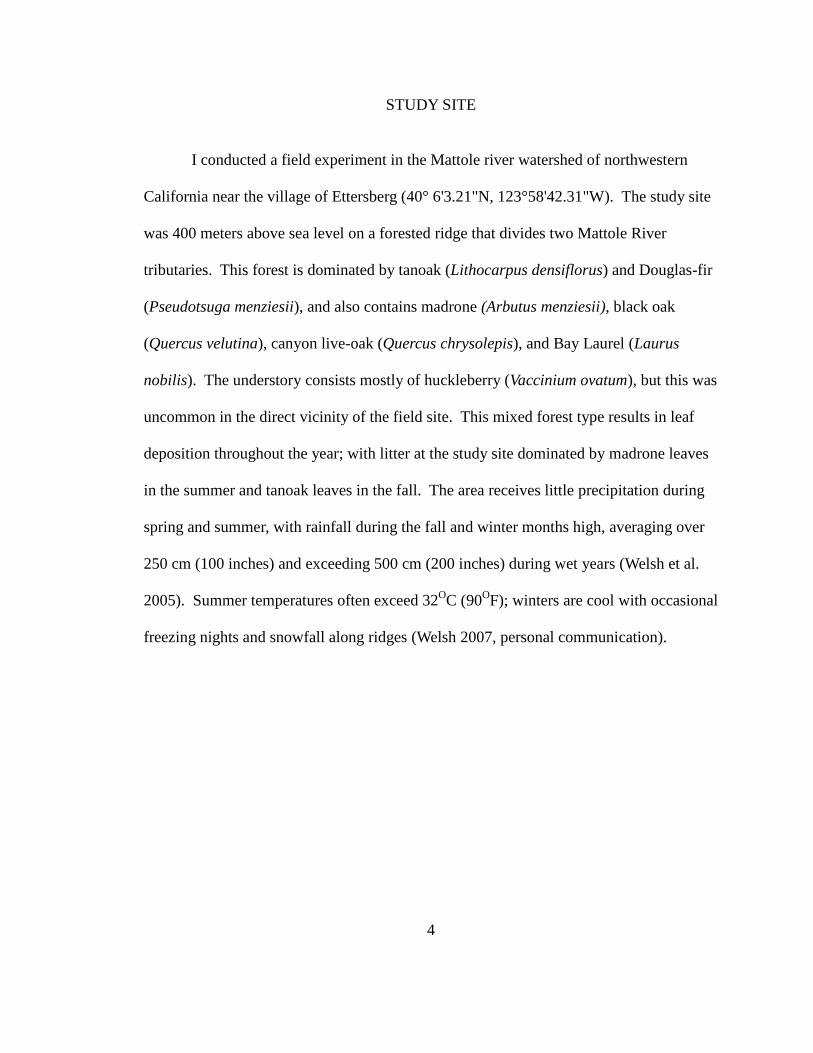
I conducted a field experiment in the Mattole river watershed of northwestern

California near the village of Ettersberg (40° 6'3.21"N, 123°58'42.31"W). The study site

was 400 meters above sea level on a forested ridge that divides two Mattole River

tributaries. This forest is dominated by tanoak (Lithocarpus densiflorus) and Douglas-fir

(Pseudotsuga menziesii), and also contains madrone (Arbutus menziesii), black oak

(Quercus velutina), canyon live-oak (Quercus chrysolepis), and Bay Laurel (Laurus

nobilis). The understory consists mostly of huckleberry (Vaccinium ovatum), but this was

uncommon in the direct vicinity of the field site. This mixed forest type results in leaf

deposition throughout the year; with litter at the study site dominated by madrone leaves

in the summer and tanoak leaves in the fall. The area receives little precipitation during

spring and summer, with rainfall during the fall and winter months high, averaging over

250 cm (100 inches) and exceeding 500 cm (200 inches) during wet years (Welsh et al.

2005). Summer temperatures often exceed 32OC (90

OF); winters are cool with occasional

freezing nights and snowfall along ridges (Welsh 2007, personal communication).

5

MATERIALS AND METHODS

To test the effects of Ensatina predation on invertebrates I conducted a controlled

salamander housing experiment over four winter months during 2007-2008 and 2008-

2009. In order to incorporate the bottom up effects of the living forest floor, salamander

barriers were installed directly into the ground (15 cm deep) where they remained,

uncovered and exposed. These barriers created 12 similar plots utilized as either controls

or treatments (six of each). I collected leaf-litter cores to quantify the invertebrates in

each plot before conducting the experiment and then at the end of each 30 day period

following the introduction of salamander treatment individuals. Leaf litter bags of a

similar composition and pre-determined dry weight were placed within each plot at the

initiation of salamander introductions and were removed 120 days later to assess the

breakdown of leaf litter in both control and treatment plots.

Experimental design

I used three experimental enclosures, each divided into four plots (1.5 m2);

creating a total of six treatment and six control plots (Figure 1). The enclosures were

constructed in situ on the forest floor. The walls were buried 15 cm deep into the litter

layer down to the mineral soil to ensure that salamanders could not escape beneath the

walls. The three enclosures were within a 12 m2 area and all three were enclosed by a

chicken wire fence 2.5 meters in height to prevent destruction or predation of Ensatina by

wildlife. Enclosures were constructed using 30 cm high metal sheets folded and attached

6

Figure 1. Experimental enclosures to assess the impacts of Ensatina on invertebrate and

litter turnover in situ at the field location near Ettersburg, California. Enclosure

dimensions were 3 m x 3 m x 23 cm, plot dimensions = 1.5 m x 1.5 m x 23 cm.

7

at the corners with steel bolts to form the perimeter and transected with a pair of metal

sheets through the center as a perpendicular bisector of each exterior wall to create four

equal-sized plots in each enclosure (Figure 1). The use of experimental field enclosures

to study food web dynamics has been criticized because it may confound predator-prey

interactions, including predator avoidance, and influx of prey from neighboring sites

(Walton 2005, Walton et al. 2006). To address these issues, the four interior walls were

equipped with two hardware cloth windows (1.5 cm mesh) measuring 10 cm in height

and 35 cm in length fastened to the sheet metal with screws to allow for arthropod

migration between the plots while preventing salamanders from moving between them.

Enclosures were equipped with a 10 cm aluminum lip around all edges fastened with

binder clips silicone glued to the underside, using duct-tape to seal the adjoining surfaces;

preventing salamanders from climbing out. The enclosures remained open at the top to

allow rainfall and leaf-litter deposition to occur naturally.

Each four-unit enclosure was systematically assigned two treatment and two

control plots with a random start, but so that no two treatment plots were adjacent. One

male Ensatina was placed in each treatment plot. Ensatina weighed at least 3.5 grams but

not more than 4.5 grams. Each plot was provided with three rough-cut Douglas-fir

boards measuring: 45 cm by 15 cm and between five and eight cm high for surface cover.

Salamanders found to already exist within enclosures were removed at the beginning of

the experiment. One treatment plot was omitted from the analysis on December 7, 2007

due to escape of the Ensatina salamander. Methodologies were approved by the

8

International Animal Care and Use Committee at Humboldt State University; protocol

number was 06/07.W.150.A.

Timing

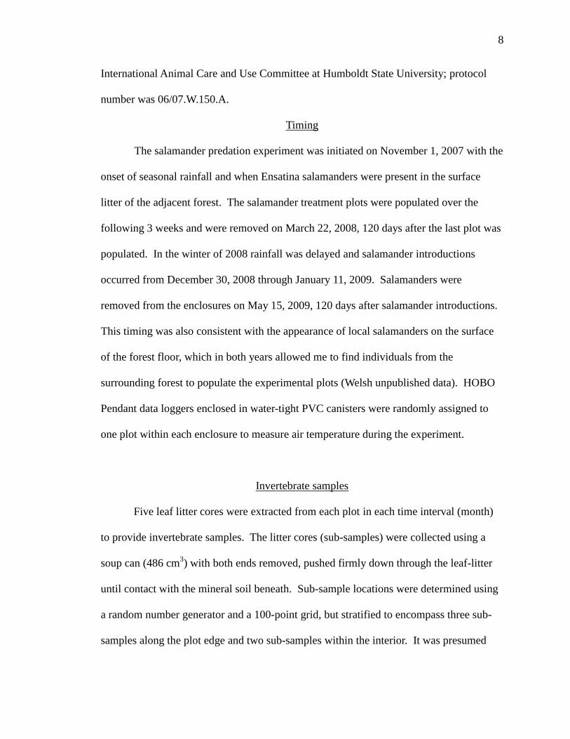
The salamander predation experiment was initiated on November 1, 2007 with the

onset of seasonal rainfall and when Ensatina salamanders were present in the surface

litter of the adjacent forest. The salamander treatment plots were populated over the

following 3 weeks and were removed on March 22, 2008, 120 days after the last plot was

populated. In the winter of 2008 rainfall was delayed and salamander introductions

occurred from December 30, 2008 through January 11, 2009. Salamanders were

removed from the enclosures on May 15, 2009, 120 days after salamander introductions.

This timing was also consistent with the appearance of local salamanders on the surface

of the forest floor, which in both years allowed me to find individuals from the

surrounding forest to populate the experimental plots (Welsh unpublished data). HOBO

Pendant data loggers enclosed in water-tight PVC canisters were randomly assigned to

one plot within each enclosure to measure air temperature during the experiment.

Invertebrate samples

Five leaf litter cores were extracted from each plot in each time interval (month)

to provide invertebrate samples. The litter cores (sub-samples) were collected using a

soup can (486 cm3) with both ends removed, pushed firmly down through the leaf-litter

until contact with the mineral soil beneath. Sub-sample locations were determined using

a random number generator and a 100-point grid, but stratified to encompass three sub-

samples along the plot edge and two sub-samples within the interior. It was presumed

9

that the plot edge might accumulate invertebrates by promoting travel along this barrier

and as such it would be important to sample this area. Sub-sample locations were not

reused. Holes generated from removing litter cores were first measured to determine

litter depth then gently collapsed to prevent soil drying and to minimize disturbance to

soil strata. The five sub-samples from each plot were combined to create the invertebrate

sample for each plot, each month. The litter removal associated with this sampling

method totaled approximately 5% of the surface area of each plot in each sampling event;

resulting in approximately 25% of the plot surface area sampled over the experiment.

The material removed from a sub-sample core was immediately placed into a

labeled quart-sized Ziploc© bag and then into a cooler to prevent the samples from

drying out or mobile invertebrates from escaping. The sub-samples were chilled but

above freezing (1-5 O

C) until they could be processed in Berlese-funnel extractions to

collect the arthropods they contained, within 48 hours. The Berlese funnels were setup

within a wooden frame approximately one square meter with 30 seven centimeter

diameter holes bored into wooden slats fitted atop the frame; each hole with a plastic

funnel attached below. The structure was designed to fit a sub-sample can within each

position such that the can would rest securely within the funnel. A hardware cloth barrier

(1.5 cm mesh) was placed at the bottom of each can to prevent soil from clogging the

funnel. A string of seven watt lights hung above the frame with one light placed within

the top of each sampling can. Each can was wrapped shut with aluminum foil to promote

the drying of samples and the downward migration of invertebrates. One dram vials

filled with 95% ethanol were placed underneath each funnel to collect invertebrates as

they fell from the litter sample. Berlese-funnel extractions received continuous heat and

10

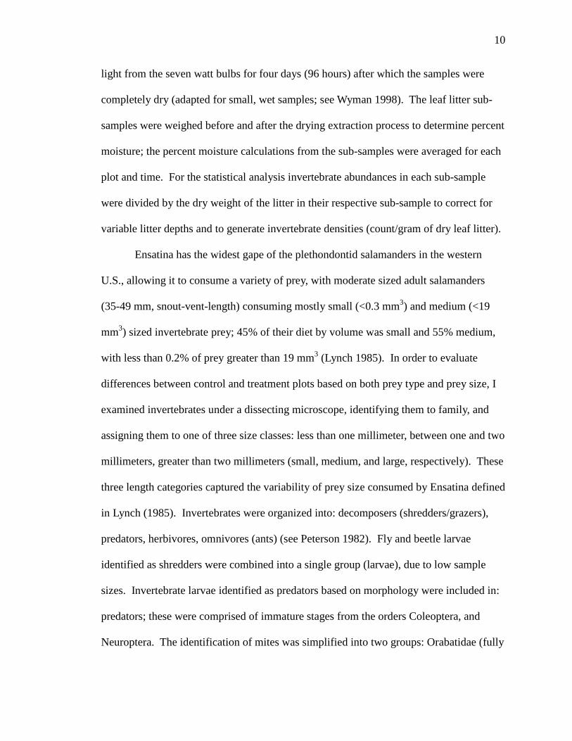
light from the seven watt bulbs for four days (96 hours) after which the samples were

completely dry (adapted for small, wet samples; see Wyman 1998). The leaf litter sub-

samples were weighed before and after the drying extraction process to determine percent

moisture; the percent moisture calculations from the sub-samples were averaged for each

plot and time. For the statistical analysis invertebrate abundances in each sub-sample

were divided by the dry weight of the litter in their respective sub-sample to correct for

variable litter depths and to generate invertebrate densities (count/gram of dry leaf litter).

Ensatina has the widest gape of the plethondontid salamanders in the western

U.S., allowing it to consume a variety of prey, with moderate sized adult salamanders

(35-49 mm, snout-vent-length) consuming mostly small (<0.3 mm3) and medium (<19

mm3) sized invertebrate prey; 45% of their diet by volume was small and 55% medium,

with less than 0.2% of prey greater than 19 mm3 (Lynch 1985). In order to evaluate

differences between control and treatment plots based on both prey type and prey size, I

examined invertebrates under a dissecting microscope, identifying them to family, and

assigning them to one of three size classes: less than one millimeter, between one and two

millimeters, greater than two millimeters (small, medium, and large, respectively). These

three length categories captured the variability of prey size consumed by Ensatina defined

in Lynch (1985). Invertebrates were organized into: decomposers (shredders/grazers),

predators, herbivores, omnivores (ants) (see Peterson 1982). Fly and beetle larvae

identified as shredders were combined into a single group (larvae), due to low sample

sizes. Invertebrate larvae identified as predators based on morphology were included in:

predators; these were comprised of immature stages from the orders Coleoptera, and

Neuroptera. The identification of mites was simplified into two groups: Orabatidae (fully

11

sclerotized) and non-Orabatidae (not or partially sclerotized). Appendix A contains a

complete list of invertebrates detected.

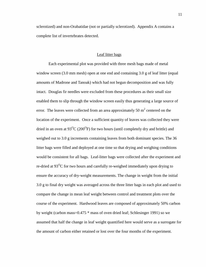
Leaf litter bags

Each experimental plot was provided with three mesh bags made of metal

window screen (3.0 mm mesh) open at one end and containing 3.0 g of leaf litter (equal

amounts of Madrone and Tanoak) which had not begun decomposition and was fully

intact. Douglas fir needles were excluded from these procedures as their small size

enabled them to slip through the window screen easily thus generating a large source of

error. The leaves were collected from an area approximately 50 m2 centered on the

location of the experiment. Once a sufficient quantity of leaves was collected they were

dried in an oven at 93OC (200

OF) for two hours (until completely dry and brittle) and

weighed out to 3.0 g increments containing leaves from both dominant species. The 36

litter bags were filled and deployed at one time so that drying and weighing conditions

would be consistent for all bags. Leaf-litter bags were collected after the experiment and

re-dried at 93OC for two hours and carefully re-weighed immediately upon drying to

ensure the accuracy of dry-weight measurements. The change in weight from the initial

3.0 g to final dry weight was averaged across the three litter bags in each plot and used to

compare the change in mean leaf weight between control and treatment plots over the

course of the experiment. Hardwood leaves are composed of approximately 50% carbon

by weight (carbon mass=0.475 * mass of oven dried leaf; Schlesinger 1991) so we

assumed that half the change in leaf weight quantified here would serve as a surrogate for

the amount of carbon either retained or lost over the four months of the experiment.

12

Statistical analysis

The samples of invertebrates yielded counts of their densities from each of the 12

plots: initially (prior to salamander introductions), and after each 30 day period following

their introductions (4 months), replicated in both years. Because invertebrate sampling

occurred within the same plots over time the samples were considered repeated measures

within each year. Walton (2005) demonstrated the significant influence of moisture on

invertebrate densities and differences in the effects of top-down regulation by a

salamander predator, therefore the distinct differences in rainfall regime between the two

years at the site warranted the analysis of each year separately. The depth of each litter

core and the amount of moisture each contained were highly correlated, requiring the

choice of only one (i.e. percent moisture) in the analysis. Air temperatures were not

included in the model because invertebrate samples were collected only once a month

which truncated temperature measurements to a scale too coarse to be meaningful.

However, the variable “month” included all effects other than moisture and

control/treatment, including temperature extremes (freezing nights, very warm days) and

trophic interactions (birth/recruitment, predation, parasitism/disease, movement).

I used a general linear model (GLM) analysis of variance that accommodated

repeated measures to test for significant effects of the three independent variables

(treatment, moisture, month), and their interactions, on each invertebrate group. The

analysis was conducted using SAS 9.2 (2008). A generalized linear model was not used

because the residual error was too large to be considered a good fit; residuals increased

consistently with increasing counts. Invertebrate counts were log transformed

[log(Count+1)] to meet the assumptions of normality. Residuals were examined to assess

13

the adequacy of these transformations. The residuals were approximately normal and

relatively constant across the predicted values following the transformation.

The response variables used in the general linear model analysis were the log

transformed counts of the density of each invertebrate family. Invertebrate families

commonly consumed by Ensatina (Bury and Martin 1973) were each broken into three

response variables (each size class) to increase the resolution of impacts to these groups.

Invertebrate families not commonly consumed by Ensatina (Bury and Martin 1973) were

each analyzed as a single response variable which included all sizes. Invertebrate

families identified as Ensatina prey, but which contained insufficient data to be analyzed

separately by size class were each treated as a single response variable that included all

sizes. Invertebrate families were also combined into functional groups to assess Ensatina

effects at a coarse level of resolution; the invertebrate decomposer group contained an

adequate sampling size which enabled the analysis of this functional group by size class.

The GLM terms for each response variable were as follows (see Table 1 for definitions):

The plot was the sampling level of the analysis, with 12 plots in total divided

equally between control and treatment, N=6. In Year One N=5 due to removal of one

treatment plot from analysis due to salamander escape. The GLM was applied once to

each invertebrate group in each year in an exploratory and not confirmatory analysis,

therefore, Bonferroni adjustments for multiple comparisons were not deemed appropriate.

The change in dry weight of the leaf litter bags from start to end were compared (control

vs. treatment) for each year using ANOVA in NCSS (Hintze 2001).

14

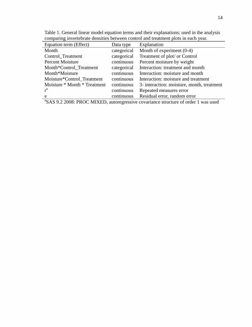
Table 1. General linear model equation terms and their explanations; used in the analysis

comparing invertebrate densities between control and treatment plots in each year.

Equation term (Effect) Data type Explanation

Month categorical Month of experiment (0-4)

Control_Treatment categorical Treatment of plot/ or Control

Percent Moisture continuous Percent moisture by weight

Month*Control_Treatment categorical Interaction: treatment and month

Month*Moisture continuous Interaction: moisture and month

Moisture*Control_Treatment continuous Interaction: moisture and treatment

Moisture * Month * Treatment continuous 3- interaction: moisture, month, treatment

ra

continuous Repeated measures error

e continuous Residual error, random error aSAS 9.2 2008: PROC MIXED, autoregressive covariance structure of order 1 was used

15

RESULTS

In Year One (2007-2008), leaf litter cores from the 10 experimental plots yielded

14,401 individual invertebrates (57.4 individuals/gram of leaf litter) from 38 families. In

Year Two (2008-2009), litter cores from the 12 plots yielded 32,721 invertebrates (253.1

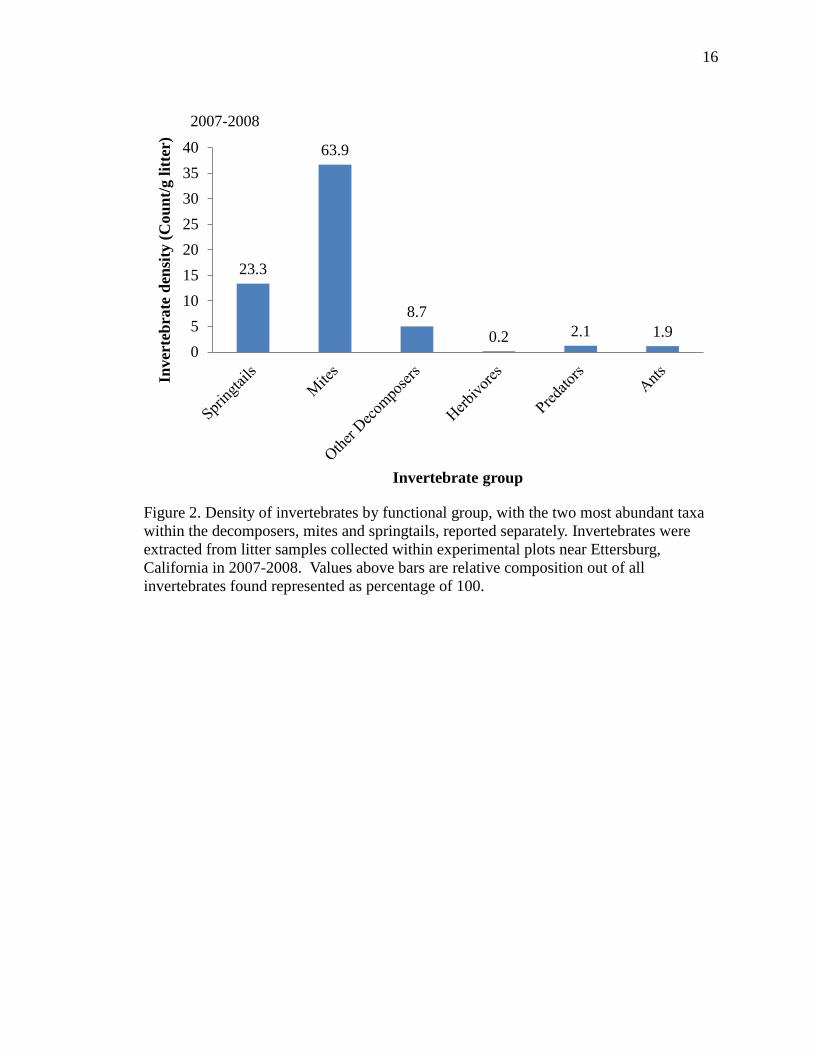
individuals/gram of litter) from 48 families (Appendix A). Invertebrates were about half

as dense in leaf litter cores during the 2007-2008 sampling year (Figure 2) as they were in

the 2008-2009 samples (Figure 3); however, the relative composition of the functional

groups was nearly identical in the two years. The majority of invertebrates found in the

leaf litter were decomposers (95%); herbivores, predators, and omnivores (ants) together

constituted a minority, comprising about 5% of all invertebrates found in litter samples in

each year. The decomposers were comprised overwhelmingly of mites (~65%), which

were almost 3 times as dense as springtails (~25%); all others constituted about 10%.

Invertebrate density was similar between control and treatment plots prior to

salamander introductions in 2007 (t=0.12, df=190, p=0.90, Figure 4) and 2008 (t=-0.05,

df=230, p=0.96, Figure 5). Invertebrate density was significantly influenced by percent

moisture of litter samples in 2007-2008 (f=17.48, df=190, p<0.0001) and 2008-2009

(f=18.52, df=230, p<0.0001, Table 2). The density of invertebrates appeared to fluctuate

with available moisture over time, in each year, with the majority of these fluctuations

attributed to small invertebrate decomposers (Table 2, Figures 4 and 5). The presence of

Ensatina did not significantly affect overall invertebrate density in 2007-2008 (f=0.03,

df=190, p=0.87) or 2008-2009 (f=0.73, df=230, p=0.39; Table 2), however, Ensatina did

influence the densities of individual invertebrate taxa in each year (see below).

16

Figure 2. Density of invertebrates by functional group, with the two most abundant taxa

within the decomposers, mites and springtails, reported separately. Invertebrates were

extracted from litter samples collected within experimental plots near Ettersburg,

California in 2007-2008. Values above bars are relative composition out of all

invertebrates found represented as percentage of 100.

23.3

63.9

8.7

0.2 2.1 1.9

0

5

10

15

20

25

30

35

40In

ver

teb

rate

den

sity

(C

ou

nt/

g l

itte

r)

Invertebrate group

2007-2008

17

Figure 3. Density of invertebrates by functional group, with the two most abundant taxa

within the decomposers, mites and springtails, reported separately. Invertebrates were

extracted from litter samples collected within experimental plots near Ettersburg,

California in 2008-2009. Values above bars are relative composition out of all

invertebrates found represented as percentage of 100.

21.7

68.8

6.1 1.1 1.8 1.4

0

25

50

75

100

125

150

175

200

Inver

teb

rate

den

sity

(C

ou

nt/

g l

itte

r)

Invertebrate group

2008-2009

18

0

0.5

1

1.5

2

2.5

3

Nov Dec Jan Feb Mar

Den

sity

of

dec

om

pose

rs

<1m

m l

on

g (

Cou

nt/

g l

itte

r)

Month

Per

cen

t li

tter

mois

ture

Ensatina introduction

0

0.5

1

1.5

2

2.5

3In

ver

teb

rate

den

sity

(C

ou

nt/

g l

itte

r)

Control Treatment

Figure 4. Mean density of all invertebrates and invertebrate decomposers <1mm on

control and treatment plots sampled at 5 monthly intervals in 2007-2008 from Mattole

field sites near Ettersburg, California. The blue line represents the percent litter moisture

in 2007-2008. Error bars are ± one standard error.

Per

cen

t li

tter

mois

ture

Moisture

Ensatina introduction

0

0.05

0.1

0.15

0.2

0.25

2007-2008

0

0.05

0.1

0.15

0.2

0.25

19

0

1

2

3

4

5

6

7

8In

ver

teb

rate

den

sity

(Cou

nt/

gli

tter

)

Control Treatment

0

1

2

3

4

5

6

7

8

Jan Feb Mar Apr May

Den

sity

of

dec

om

pose

rs

<1m

m l

on

g (

Cou

nt/

g l

itte

r)

Month

Per

cen

t li

tter

mois

ture

Ensatina introduction

Per

cen

t li

tter

mois

ture

Moisture

0

0.05

0.1

0.15

0.2

0.25

0.3

0.35

0

0.05

0.1

0.15

0.2

0.25

0.3

0.35

Figure 5. Mean density of all invertebrates and invertebrate decomposers <1mm on

control and treatment plots sampled at 5 monthly intervals in 2008-2009 from Mattole

field sites near Ettersburg, California. The blue line represents the percent litter moisture

in 2008-2009. Error bars are ± one standard error.

2008-2009

Ensatina introduction

20

Table 2. Analysis of the effects of salamander predation (Control_Treatment), moisture, month, and the interaction of

month*moisture, on invertebrate functional groups by size class in two years using a general linear model. Data were analyzed

separately by group, size, and year. Results indicated with – were not statistically significant at α = 0.1.

Moisture Month Month*Moisture Control_Treatment

Group Size Year F-value P-value F-value P-value F-value P-value F-value P-value

Decomposers <1 mm 1 10.31 0.002 - - 2.09 0.083 - -

<2 mm 1 9.91 0.002 - - - - - -

>2 mm 1 - - - - - - - -

<1 mm 2 20.94 0.000007 5.01 0.001 5.56 0.0003 - -

<2 mm 2 3.92 0.049 3.18 0.014 4.41 0.002 - -

>2 mm 2 22.66 0.000003 2.56 0.039 2.37 0.053 - -

Omnivores (Ants) All sizes 1 14.24 0.0002 - - - - - -

All sizes 2 - - - - - - - -

Predators All sizes 1 3.64 0.058 - - - - - -

All sizes 2 - - - - 2.02 0.092 - -

Herbivores All sizes 1 - - - - - - - -

All sizes 2 - - 9.81 0.000 - - - -

All invertebrates All sizes 1 17.48 0.00004 2.09 0.08 2.23 0.07 - -

All sizes 2 18.52 0.00002 4.84 0.0009 6.06 0.0001 - -

21

Ensatina effects on invertebrate taxa

In 2007-2008 the densities of 10 invertebrate taxa were significantly affected by

Ensatina presence (6 decreased, 4 increased; Table 3); in contrast, only three taxa were

affected by Ensatina in 2008-2009, all of which increased on treatment compared to

control plots. Two of the taxa which declined on treatment plots in Year One, rebounded

to densities higher than controls following the initial declines (Figure 6). There were no

significant declines on treatment plots in Year Two, although two taxa that had declined

significantly in Year One showed declining trends in the Year Two but did not achieve

statistical significance: medium Entomobryidae springtails and beetles (see Figure 15).

In Year One (2007-2008) the density of medium Entomobryidae springtails

(f=3.32, df=190, p=0.07), medium beetles (f=6.39, df=190, p=0.01), and large larval

shredders (f=2.79, df=190, p=0.09) each declined significantly on plots with Ensatina in

month one and two (Table 3, Figure 6). The density of medium Entomobryidae

springtails and large larval shredders each increased in month three following their

declines, to a level greater than adjacent control sites (Figure 6). Large larval shredders

remained greater than controls into month four (Figure 6). The density of earwigs

declined significantly on treatments in months one and four (f=3.57, df=190, p=0.06,

Figure 7). The density of medium larval shredders remained similar between control and

treatment plots in month one, but were found in significantly higher densities on

treatments in months two and four (f=3.85, df=190, p=0.05, Table 3, Figure 6).

The density of small Orabatidae mites increased significantly on plots with

Ensatina within the first month following Ensatina introduction and again in month four

(f=2.69, df=190, p=0.32, Table 3, Figure 8); interaction between treatment and month.

22

Table 3. Analysis of the effects of salamander presence (Control_Treatment), and their interactions with moisture and time interval on

invertebrate taxa in two years using a general linear model. Data were analyzed separately by taxon, size class, and year. Results

indicated with - were not statistically significant at α = 0.1.

Control_Treatment Moisture*Treatment Month*Treatment Month*Moisture*Treatment

Taxa Size Year F-value P-value F-value P-value F-value P-value F-value P-value

Springtailsa <2 mm 1 3.32 0.070 3.52 0.062 - - - -

<2 mm 2 - - - - - - - -

Adult Beetles <2 mm 1 - - 5.27 0.023 - - - -

<2 mm 2 - - - - - - - -

Larvaeb

<2 mm 1 3.85 0.051 - - - - - -

>2 mm 1 2.79 0.096 - - - - - -

>2 mm 2 - - - - - - - -

Mites_Orabatid. <1 mm 1 - - - - 2.69 0.032 2.16 0.075

<2 mm 2 - - - - - - - -

Spiders <2 mm 1 2.79 0.097 2.77 0.098 - - - -

Earwigs All sizes 1 3.57 0.060 3.27 0.072 - - - -

Ants All sizes 1 - - - - 2.79 0.27 4.09 0.003

Millipedes All sizes 1 - - - - 2.31 0.059 3.36 0.01

True bugs All sizes 1 - - - - 2.71 0.03 3.52 0.008

Bark lice All sizes 2 3.04 0.083 - - - - - -

Worms All sizes 2 - - 3.40 0.066 - - - -

Pseudoscorpions All sizes 2 - - - - - - 2.07 0.086 aSpringtails determined to be members of the family Entomobryidae by examination of morphological features

bLarvae determined to be saprophytic shredders by examination of morphology, includes immature stages of: Coleoptera, Diptera

23

0

0.01

0.02

0.03

0.04

0.05

0.06

Den

sity

of

ad

ult

bee

tles

<2 m

m l

on

g

(Cou

nt/

g l

itte

r) Ensatina introduction

0

0.01

0.02

0.03

0.04

0.05

0.06

Den

sity

of

larv

ae

>2m

m

lon

g (

Cou

nt/

g l

itte

r)

0

0.01

0.02

0.03

0.04

0.05

0.06

Nov Dec Jan Feb Mar

Den

sity

of

larv

ae

<2m

m

lon

g (

Cou

nt/

g l

itte

r)

Month

Ensatina introduction

0

0.01

0.02

0.03

0.04

0.05

0.06D

ensi

ty o

f E

nto

mob

ryid

ae

spri

ngta

ils

<2 m

m l

on

g

(Cou

nt/

g l

itte

r)

Control TreatmentEnsatina introduction

Figure 6. Mean density of: Entomobryidae springtails <2mm, beetles <2mm, larvae

>2mm, and larvae <2mm on control and treatment plots sampled at 5 monthly intervals in

2007-2008 from Mattole field sites near Ettersburg, California. Error bars are ± one

standard error.

Ensatina introduction

2007-2008

24

Figure 7. Mean density of earwigs on control and treatment plots sampled at 5 monthly

intervals in 2007-2008 from Mattole field sites near Ettersburg, California. Error bars are

± one standard error.

0

0.001

0.002

0.003

0.004

0.005

0.006

0.007

0.008

Nov Dec Jan Feb Mar

Earw

ing d

ensi

ty (

Cou

nt/

g l

itte

r)

Month

Control Treatment

Ensatina introduction

2007-2008

25

Figure 8. Mean density of Orabatidae mites <1mm on control and treatment plots

sampled at 5 monthly intervals in 2007-2008 from Mattole field sites near Ettersburg,

California. Error bars are ± one standard error.

0

0.2

0.4

0.6

0.8

1

1.2

Nov Dec Jan Feb Mar

Den

sity

of

Ora

ba

tid

ae

mit

es

<1 m

m l

on

g (

Cou

nt/

g l

itte

r)

Month

Control Treatment

Ensatina introduction

2007-2008

26

In Year One medium spiders were found at greater density on plots with Ensatina

compared to controls throughout the four months of the experiment (f=2.79, df=190,

p=0.097, Table 3, Figure 9). The density of ants was low on all plots through the first

three months of Year One, however decreased significantly on plots with Ensatina in the

final month of the experiment, indicating the significant interaction between month,

moisture, and treatment (f=4.09, df=190, p=0.003, Figure 10). The density of millipedes

was greater on treatment plots in months one, two, and four (f=3.36, df=190, p=0.01,

Figure 11). The density of true bugs (Hemiptera) was significantly lower on treatments in

Year One (f=3.52, df=190, p=0.008; Table 3, Figure 12), however, also rare (0.00005%

of all invertebrates), likely influencing comparisons and significance.

In Year Two the density of barklice (Psocoptera) increased significantly on plots

with Ensatina compared to controls in months two and four (f=3.04, df=230, p=0.08;

Table 3, Figure 13). The density of worms (Annelida) increased significantly on plots

with Ensatina over controls during months two and four, indicating an interaction

between treatment and moisture (f=3.4, df=230, p=0.07; Table 3, Figure 13). The density

of Pseudoscorpions increased significantly on plots with Ensatina in month one and again

in months three and four of Year Two (f=2.07, df=230, p=0.09; Table 3, Figure 14);

indicating the interaction between month, moisture, and treatment.

During the latter three months of Year Two the densities of four taxa which

differed significantly between control and treatment in Year One (Fig. 6, Table 3) showed

a similar trend in the second year: medium Entomobryidae springtails, medium beetles,

medium Orabatidae mites, and large larval shredders. The differences in densities of

these taxa did not achieve statistical significance in the second year (Figure 15, Table 3).

27

Figure 9. Mean density of spiders <2mm on control and treatment plots sampled at 5

monthly intervals in 2007-2008 from Mattole field sites near Ettersburg, California. Error

bars are ± one standard error.

0

0.001

0.002

0.003

0.004

0.005

0.006

0.007

Nov Dec Jan Feb Mar

Den

sity

of

spid

ers

<2 m

m l

on

g

(Co

un

t/g

lit

ter)

Month

Control Treatment

2007-2008

Ensatina introduction

28

Figure 10. Mean density of ants on control and treatment plots sampled at 5 monthly

intervals in 2007-2008 from Mattole field sites near Ettersburg, California. Error bars are

± one standard error.

00.020.040.060.08

0.10.120.140.160.18

0.2

Nov Dec Jan Feb Mar

An

t d

ensi

ty (

Cou

nt/

g l

itte

r)

Month

Control Treatment

Ensatina introduction

2007-2008

29

Figure 11. Mean density of millipedes on control and treatment plots sampled at 5

monthly intervals in 2007-2008 from Mattole field sites near Ettersburg, California. Error

bars are ± one standard error.

0

0.005

0.01

0.015

0.02

0.025

0.03

0.035

0.04

Nov Dec Jan Feb Mar

Mil

lip

ede

den

sity

(C

ou

nt/

g l

itte

r)

Month

Control Treatment

Ensatina introduction

2007-2008

30

Figure 12. Mean density of true bugs (Hemiptera) on control and treatment plots sampled

at 5 monthly intervals in 2007-2008 from Mattole field sites near Ettersburg, California.

Error bars are ± one standard error.

0.000

0.001

0.001

0.002

0.002

0.003

0.003

Nov Dec Jan Feb Mar

Den

sity

of

tru

e b

ugs

(Cou

nt/

g l

itte

r)

Month

Control Treatment

Ensatina introduction

2007-2008

31

0

0.01

0.02

0.03

0.04

0.05

Jan Feb Mar Apr May

Worm

den

sity

(C

ou

nt/

g l

itte

r)

Month

0

0.01

0.02

0.03

0.04

0.05B

ark

lice

den

sity

(C

ou

nt/

g l

itte

r) Control Treatment

Ensatina introduction

Figure 13. Mean density of: barklice (Psocoptera) and worms (Annelida) on control and

treatment plots sampled at 5 monthly intervals in 2008-2009 from Mattole field sites near

Ettersburg, California. Error bars are ± one standard error.

2008-2009

Ensatina introduction

32

Figure 14. Mean density of Pseudoscorpions on control and treatment plots sampled at 5

monthly intervals in 2008-2009 from Mattole field sites near Ettersburg, California. Error

bars are ± one standard error.

0.000

0.002

0.004

0.006

0.008

0.010

0.012

0.014

0.016

Jan Feb Mar Apr May

Pse

ud

osc

orp

ion

den

sity

(Co

un

t/g

lit

ter)

Month

Control TreatmentEnsatina introduction

2008-2009

33

0.000.020.040.060.080.100.120.140.160.18

Den

sity

of

ad

ult

bee

tles

<2 m

m l

on

g

(Cou

nt/

g l

itte

r)

0.00

0.02

0.04

0.06

0.08

0.10

0.12

0.14

0.16

0.18

Den

sity

of

En

tom

ob

ryid

ae

spri

ngta

ils

<2 m

m l

on

g

(Co

un

t/g

lit

ter)

Control Treatment

0.000.020.040.060.080.100.120.140.160.18

Den

sity

of

Ora

bati

dae

mit

es <

2m

m l

on

g

(Cou

nt/

g l

itte

r)

0.000.020.040.060.080.100.120.140.160.18

Jan Feb Mar Apr May

Den

sity

of

larv

ae

>2 m

m l

on

g

(Cou

nt/

g l

itte

r)

Month

Figure 15. Mean density of: Entomobryidae springtails <2mm, beetles <2mm, Orabatidae

mites <2mm and larvae >2mm, on control and treatment plots sampled at 5 monthly

intervals in 2008-2009 from Mattole field sites near Ettersburg, California. Error bars are

± one standard error.

Ensatina introduction

Ensatina introduction

Ensatina introduction

Ensatina introduction 2008-2009

34

Leaf-litter

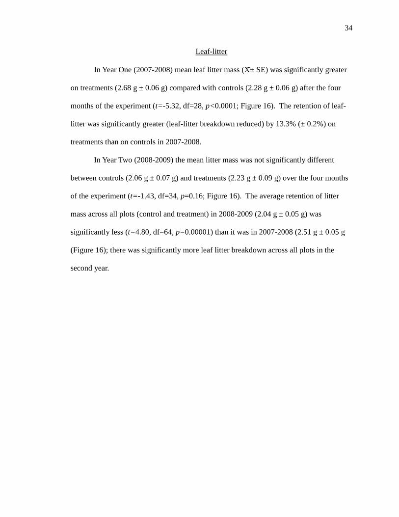
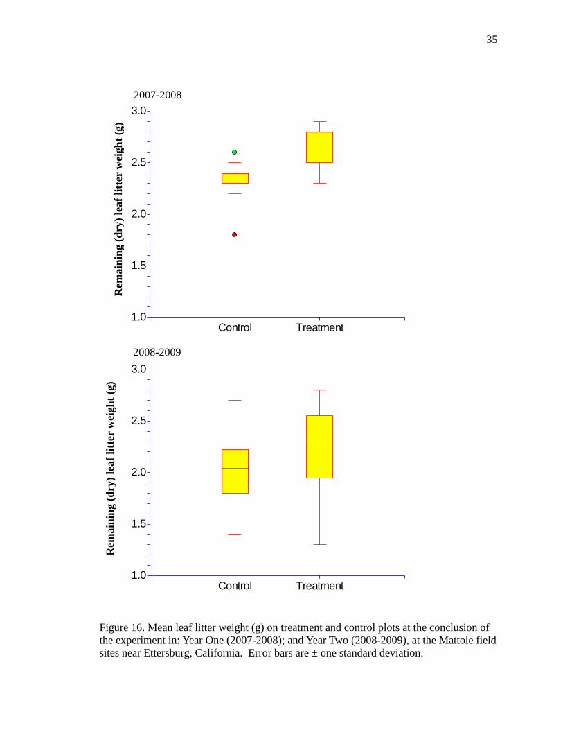
In Year One (2007-2008) mean leaf litter mass (Χ± SE) was significantly greater

on treatments (2.68 g ± 0.06 g) compared with controls (2.28 g ± 0.06 g) after the four

months of the experiment (t=-5.32, df=28, p<0.0001; Figure 16). The retention of leaf-

litter was significantly greater (leaf-litter breakdown reduced) by 13.3% (± 0.2%) on

treatments than on controls in 2007-2008.

In Year Two (2008-2009) the mean litter mass was not significantly different

between controls (2.06 g ± 0.07 g) and treatments (2.23 g ± 0.09 g) over the four months

of the experiment (t=-1.43, df=34, p=0.16; Figure 16). The average retention of litter

mass across all plots (control and treatment) in 2008-2009 (2.04 g ± 0.05 g) was

significantly less (t=4.80, df=64, p=0.00001) than it was in 2007-2008 (2.51 g ± 0.05 g

(Figure 16); there was significantly more leaf litter breakdown across all plots in the

second year.

35

Figure 16. Mean leaf litter weight (g) on treatment and control plots at the conclusion of

the experiment in: Year One (2007-2008); and Year Two (2008-2009), at the Mattole field

sites near Ettersburg, California. Error bars are ± one standard deviation.

1.0

1.5

2.0

2.5

3.0

Control Treatment

1.0

1.5

2.0

2.5

3.0

Control Treatment

Rem

ain

ing (

dry

) le

af

litt

er w

eigh

t (g

) R

em

ain

ing (

dry

) le

af

litt

er w

eigh

t (g

)

2007-2008

2008-2009

36

DISCUSSION

The great abundances of terrestrial salamanders in North American forests (e.g.,

Burton and Likens 1978a, Welsh and Lind 1992, Petranka and Murray 1999) implies an

important role in forest floor food web dynamics through predation on invertebrate

assemblages including larval shredders and detrital grazers (beetles and springtails).

Members of the invertebrate shredder guild (larvae and worms) physically tear organic

material such as leaf litter, conifer needles, and wood on the forest floor into smaller

pieces, which are then processed through their gut, inoculated with microflora, and

utilized by microfauna (Gist and Crossley 1975). The small decomposers (mites,

springtails, and nematodes [together microfauna]) directly mediate the primary

productivity of this microfloral resource by fulfilling three ecological functions: grazing,

spreading propogules, and preying on one another (McBrayer and Reichle 1971, Singh

1977). Ultimately, this often dense microscopic layer of primary and secondary

consumers converts primary microfloral productivity and waste into invertebrate

biomass, effectively transferring energy from forest materials up the food web and

simultaneously recharging soil nutrients, including carbon and nitrogen, for plant growth

(McBrayer and Reichle 1971, Gist and Crossley 1975, Singh 1977). Ensatina predation

on these two critical components of the decomposition food web (grazers, shredders)

indicates the potential for terrestrial salamanders to have a top down influence on the

processes of nutrient cycling and carbon storage in forests.

While Ensatina preys on many of these invertebrates, exerting a top-down

influence on the rate of litter breakdown, this relationship can be affected by moisture.

37

Detrital food web processes respond directly to moisture by increasing the densities of

invertebrate shredders, grazers, and microfloral growth (Wardle 2002), which increases

the rate of leaf litter breakdown (Gist and Crossley 1975, Singh 1977). In Year Two

(2008-2009) there was an initial high pulse of moisture within the first two months of the

experiment, probably resulting in the detection of twice as many invertebrates in litter

samples than in Year One. Consistent with this pulse of enhanced activity, leaf litter

breakdown was greater in Year Two than it was in Year One. Furthermore, significant

salamander effects on invertebrate densities were fewer in Year Two: three taxa increased

in Ensatina presence (barklice, worms, pseudoscorpions; indirect effects); compared to

six taxa which decreased (medium Entomobryidae springtails, medium beetles, earwigs,

large larval shredders, ants, true bugs; direct effects) and four taxa which increased (small

Orabatidae mites, medium spiders, medium larva, millipedes; indirect effects), Year One.

In Year One, the direct and indirect effects of Ensatina presence on the

invertebrate assemblage was apparent within the first month of the experiment. The

densities of three microfloral grazers: medium Entomobryidae springtails, medium

beetles and earwigs each decreased immediately following Ensatina introduction. While

simultaneously the density of a small microfloral grazer increased: Orabatidae mites less

than one millimeter long. The removal of many of these larger grazers by Ensatina

would have likely opened up primary resources for the smaller and more numerous mites,

allowing them to capitalize on these resources and increase in density (competitive

release). A similar relationship was found with Plethodon cinereus where decreases in

the abundance of Entomobryidae springtails on salamander plots resulted in an increase

in mites and Podomorphic springtails (Walton and Steckler 2005). Rooney (2000) and

38

Walton et al. (2006) also described a similar release of Podomorphic springtails in the

presence of this salamander. In my study, the larger and highly mobile millipedes (a

microfloral grazer) also apparently capitalized on available microfloral resources,

increasing significantly in density on Ensatina plots. Large larval shredders decreased on

Ensatina plots in the first two months, allowing medium larval shredders to increase.

Consistent with the reduced densities of large larval shredders, and microfloral

grazers (springtails, beetles, earwigs) on treatments in Year One was an increase to mean

leaf litter retention by 13.3%, compared to control plots. Consistent with the pulse of

moisture early in the experiment in Year Two, and the high invertebrate densities in that

year, was an increase in the breakdown of litter across all plots, compared to Year One.

Consequently, the salamander treatment plots showed a lack of statistically significant

declines to invertebrate densities and an insignificant retention of litter on treatment plots

in Year Two. While mean dry weight of litter retained on treatments was 5% greater than

controls in Year Two, which may indicate the consumption of invertebrate decomposers

by Ensatina, there was an insufficient effect to achieve statistical significance.

With a single Ensatina salamander per 1.5 m2 treatment plot, the increased

invertebrate densities in Year Two probably decreased the likelihood of a single

salamander being able to consume enough invertebrates to achieve a statistically

significant decline. However, it appears that these Ensatina did consume high numbers of

medium Entomobryidae springtails, beetles, and mites in Year Two despite the lack of

statistically significant differences. Evidence of this is apparent in the indirect effect on a

small microfloral grazer: barklice (Psocoptera) which increased in density on plots with

Ensatina in month two; precisely when the densities of these three grazers (springtails,

39

beetles, mites) began to fluctuate on treatments. By month four barklice density was

three times greater on plots with Ensatina than on controls, indicating the compounding

indirect effects of Ensatina predation on larger microfloral grazers (medium-sized

Entomobryidae springtails, beetles, and mites) in the last three months of the experiment

in Year Two (2008-2009). Walton (2005) also observed increases in barklice on treatment

plots, apparently due to this competitive release phenomenon.

Gnaedinger and Reed (1948) reported the stomachs of 21 Ensatina contained in

decreasing frequency: springtails, spiders, millipedes, centipedes, beetles, larvae, and

mites, followed by pill bugs, thrips, and wasps. Bury and Martin (1973) found the

stomachs of 37 Ensatina contained in decreasing frequency: springtails, spiders, beetles,

millipedes, pill bugs, larvae, ants, and mites; with several other taxa including centipedes

and pseudoscorpions found in fewer than 5% of stomachs. In both studies the most

frequently consumed invertebrates included springtails, spiders, beetles, and larvae; the

densities of each differed in the presence of Ensatina in this study.

While I did not detect significant declines to invertebrate predators (possibly due

to small sample sizes), there was evidence of an indirect increase to an intermediate

invertebrate predator in each year (meso-predator release [Richie and Johnson 2009]). In

Year One medium spiders occurred in higher densities on plots with Ensatina compared

to controls. In Year Two Pseudoscorpions occurred in higher densities on plots with

Ensatina compared to controls. Gnaedinger and Reed (1948) and Bury and Martin (1973)

indicated spiders as an important food source for Ensatina; Ensatina predation on large

spiders may explain the increase in density of medium spiders on treatment plots in Year

One (2007-2008) and Pseudoscorpions in Year Two (2008-2009).

40

The influence of moisture and prey density

In Year One the density of invertebrates was high prior to introduction of

Ensatina, and was quite low on all plots in the first month following Ensatina population.

The density of invertebrates gradually increased from a low in month one through month

four of 2007-2008, apparently, as the percent moisture of litter samples increased. In the

first two months of the first year Ensatina appeared to capitalize on select invertebrates:

large larval shredders, medium Entomobryidae springtails, medium beetles, and earwigs.

By month three the significant differences (control vs. treatment) to these four taxa were

no longer apparent and at least two taxa: medium Entomobryidae springtails and large

larval shredders began to increase to densities higher than controls. In months three and

four invertebrate densities continued to increase and significant differences to these select

taxa disappeared: only earwigs and ants were less dense on treatments in month four.

In Year Two (2008-2009) invertebrate density was much higher than in Year One

(2007-2008) and I failed to detect any statistically significant declines to invertebrate taxa

on the salamander plots in Year Two (Tables 2 and 3). However, a statistically significant

indirect effect of Ensatina presence (e. g. increased density of barklice) suggests Ensatina

did consume invertebrate microfloral grazers (e. g. medium Entomobryidae springtails,

beetles, and Orabatidae mites) during months two-four of Year Two. Furthermore, these

latter three months of Year Two coincide with the decline of moisture in litter samples

and declining invertebrate density. This may have forced Ensatina to be more selective of

prey species as availability of prey decreased (Jaeger and Barnard 1981); similar to

Stamps et al. (1981) and Diaz and Carrascal (1993) whom found prey selection decrease

and eventually disappear as prey availability increased for insectivorous lizards.

41

Ensatina and optimal foraging theory

Optimal foraging theory states that predators will maximize gains and minimize

efforts by first selecting prey which provide the most energy gained per energy invested

(most profitable) and then broadening that selection to include less profitable prey as the

more preferred prey decline in density (Emlen 1966). This is based on an energy limited

model developed primarily for endothermic predators with high caloric requirements.

Salamanders are poikilotherms with low energetic requirements (Pough 1980); Ensatina

is more efficient than an endothermic insectivore (e. g. birds utilize 90% of calories for

respiration) at converting ingested calories into biomass (Burton and Likens 1975, Pough

1983). The low energetic requirements of Ensatina allow it to include abundant prey

even when energetically less profitable (Jaeger and Barnard 1981, Stamps et al. 1981,

Diaz and carascal 1993), and consider the relative nutritional qualities (complimentary

amino acids, etc.) of different taxa (Pulliam 1975, Stamps et al. 1981, Mayntz and Toft

2001). These circumstances enabled Ensatina to modulate foraging behaviors (prey

selection) in response to environmental conditions (moisture, prey density).

Ensatina is a sit-and-wait predator that invests little energy in foraging behavior so

a majority of foraging cost is inherent in the relative percentage of exoskeleton chitin in

each invertebrate taxa consumed (Jaeger 1990, Diaz and Carrascal 1993). A regression

analysis comparing handling time to prey size (mean dry mass) found relatively shallow

slopes (slow increase in handling time with size) for particularly round and/or soft bodied

taxa: true bugs, larvae, flies, and spiders but steep slopes (handling times increased

rapidly with size) for highly chitinized and elongated taxa: crickets, beetles, ants, etc.

(Jaeger 1990, Diaz and Carrascal 1993). Entomobryidae springtails are armored with

42

hairs and an enlarged dorsal segment which may place them in the high chitin group,

along with beetles and ants. Medium Entomobryidae springtails and beetles seem to be

important prey types for Ensatina in forests of Northern coastal California as they were

consumed in each year. Large beetles and springtails although common in samples

(appendix A) were not significantly reduced by Ensatina, compared to the medium size

class of each which were significantly reduced in the first two months of Year One.

Large larval shredders were important prey for Ensatina during the first two months of

Year One in particular, when prey density was the lowest recorded during this study. This

is in contrast to medium larval shredders which increased on treatments at the same time.

Temperate invertebrate communities are highly skewed towards smaller species

which can provide an ample prey base for small insectivores (Whitaker 1952, Stamps et

al. 1981). Jaeger (1980) confirms that prey are only very rarely limiting for terrestrial

salamanders, but rather may become temporarily unavailable due to low moisture or high

temperatures which can threaten salamanders with desiccation, suggesting moisture

availability may influence Ensatina foraging behaviors. During the first two months of

Year One, invertebrate density was slowly increasing from a low point and Ensatina

consumed prey within energetically favorable taxa (large larval shredders, medium

Entomobryidae springtails and beetles). In month three of Year One Ensatina did not

significantly impact these groups, and as moisture and invertebrate density approached a

peak for the experiment in month four, Ensatina consumed ants and earwigs (high chitin).

It may be that relatively limited prey availability in Year One influenced Ensatina

to consume more energetically advantageous prey (calories/cost) to maintain a positive

energy budget (e.g., Jaeger 1990, Diaz and Carrascal 1993). This may have become less

43

important in months three and four as prey density increased. Alternatively, but not

exclusively, it may be that the consumption of prey under cover objects during periods of

relatively low moisture (Jaeger 1980) influenced Ensatina to capitalize on particular taxa

commonly encountered under the cover provided (beetles, Entomobryidae springtails,

larvae). The increased moisture of months three and four of Year One may have enabled

Ensatina to explore more ground during foraging and consume a wider variety of prey.

These two phenomena were likely included in the dynamics of Year Two as well,

where top-down salamander effects did not significantly decrease the densities of any

invertebrate taxa: with moisture and invertebrate densities high there was nothing to limit

the foraging behaviors of Ensatina. Furthermore, the significant indirect effect of

Ensatina presence, which increased the density of barklice, first occurred in month two

and again in month four when moisture and invertebrate density were each most limited

in Year Two. The early pulse of moisture in Year Two may have limited the ability of

Ensatina to regulate the invertebrate community (bottom-up versus top-down forces) and

indirectly influence a greater retention of leaf litter. The differences I found between

years in the regulation of invertebrate densities by salamanders due to variation in

moisture is consistent with Walton (2005), who also found the downward effects of a

woodland salamander on invertebrates to be ameliorated by moisture. The ability of

moisture to influence the effects of top-down regulation (top-down cascades) has been

well documented for several other insectivorous predators (e.g., Anolis lizards [Spiller

and Schoner 1995]; arboreal birds [Bridgeland et al. 2010]), including terrestrial

salamanders in the Midwest (Walton 2005).

44

CONCLUSIONS AND RECOMMENDATIONS

Soils are the third largest active carbon pool globally (2,400 Pg of carbon in the

top 2 m) after the lithosphere and hydrosphere (Eshel et al. 2007); representing the largest

terrestrial reservoir of carbon (Zhou 2006, Hungate et al. 2009), especially in temperate

forests of the northern hemisphere (Beedlow 2004), where woodland salamanders are so

abundant and diverse. My results and others (Wyman 1998) indicate that terrestrial

salamanders play an ecologically dominant role at the soil-leaf litter interface of forested

ecosystems of temperate North America by promoting nutrient cycling and increasing the

retention of litter which stores energy, nutrients (nitrogen), and minerals including carbon

(Davic and Welsh 2004). The critical role of predators in maintaining ecosystem

functionality is now recognized (Richie and Johnson 2009, Estes et al. 2011). Terrestrial

salamanders clearly serve as predators in forested ecosystems, with the ability to generate

top-down effects on the invertebrate assemblage and increase the retention of leaf litter,

fostering storage of material for decomposition and increasing carbon buildup in the soil.

Further research is needed on the relative influences of sympatric terrestrial

salamanders on the detrital food web and on each other, as they relate to environmental

factors and leaf litter retention/turnover. As climatic variables continue to respond to the

effects of global climate change we need to continue to address the role of ecologically

dominant species like Ensatina in response to the impacts of climate extremes on forested

ecosystems. Increasing our understanding of the ecological linkages within these forests

can enhance our ability to better manage this resource while mitigating the effects of

anthropogenic climate change, in order to maintain these life-sustaining environments.

45

LITERATURE CITED

Beard, K. H., A. K. Eschtruth, K. A. Vogt, D. J. Vogt, and N. Scatena. 2003. The effects

of the frog Eleutherodactylus coqui on invertebrates and ecosystem processes at

two scales in the Luquillo experimental forest, Puerto Rico. Journal of Tropical

Ecology 19:607-617.

Beedlow, P. A., D. T. Tingey, D. L. Phillips, W. E. Hogsett, and D. M Olszyk. 2004.

Rising atmospheric CO2 and carbon sequestration in forests. Frontiers in Ecology

and Environment 2:315-322.

Benrong, C. and D. H. Wise. 1999. Bottom up limitation of predaceous arthropods in a

detritus based terrestrial food web. Ecological Society of America 80:761-772.

Bridgeland, W. T., P. Beier, T. Kolb, and T. G. Whitham. 2010. A conditional trophic

cascade: birds benefit faster growing trees with strong links between predators

and plants. Ecological Society of America 91(1):73-84.

Bury, R. B. and M. Martin. 1973. Comparative studies on the distribution and foods of

Plethodontid salamanders in the redwood region on Northern California. Journal

of Herpetology 7:331-335

Burton, T. M. and G. E. Likens. 1975a. Energy flow and nutrient cycling in salamander

populations in the Hubbard Brook experimental forest, New Hampshire. Ecology

56:1068-1080.

Burton, T. M. and G. E. Likens. 1975b. Salamander Populations and Biomass in the

Hubbard Brook Experimental Forest, New Hampshire. Copeia 3:541-546.

Chernova, N. M., A. I. Bokova, E. V. Varshav, N. P. Goloshcapova, and Y. Y. Savenkova.

2007. Zoophagy in Collembola. Entomological Review 87:799-811.

Davic, R. D. and H. Welsh, Jr. 2004. On the Ecological Roles of Salamanders. Annual

Review of Ecology and Evolutionary Systems 35:405-435.

Diaz, J. A. and L. M. Carrascal. 1993. Variation in the effect of profitability on prey size

selection by the Lacertid lizard Psammodromus algirus. Oecologia 94(1): 23-29.

Drift, J. v. d. and E. Jansen. 1977. Grazing of springtails on hyphal mats and its

influence on fungal growth and respiration. Ecological Bulletins 25:203-209.

Emlen, J. M. 1966. The role of time and energy in food preference. American Naturalist

100:611-617.

46

Eshel, G., P. Fine, and M. J. Singer. 2007. Total soil carbon and water quality: an

implication for carbon sequestration. Soil and Water Management and

Conservation 71: 397-405.

Gist C. S. and D. A. Crossley Jr. 1975. The litter arthropod community in a Southern

Appalachian hardwood forest: numbers, biomass, and mineral element content.

American Midland Naturalist, 93(1):107-122.

Gnaedinger, L. M. and C. A. Reed. 1948. Contribution to the natural history of the

Plethodont salamander Ensatina eschscholtzii. Copeia 3:187-196.

Gruner, D. S. 2004. Attenuation of top down and bottom up forces in a complex

terrestrial community. Ecology 85:3010-3022.

Hairston, N. G. sr., F. E. Smith, and L. B. Slobodkin. 1960. Community structure,

population control, and competition. American Naturalist 94:421-425.

Hairston N. G. Jr. and N. G. Hairston Sr. 1997. Does food web complexity eliminate

trophic level dynamics? The American Naturalist 149:1001-1007.

Halaj, J. and D. H. Wise. 2002. Impact of a detrital subsidy on trophic cascades in a

terrestrial grazing food web. Ecology 83:3141-3151.

Hickerson, C.-A. M. C. D. Anthony, and G. A, Wicknick. 2004. Behavioral interactions

between salamanders and centipedes: competition in divergent taxa. Behavioral

Ecology 15:679-686

Hintze, J. 2001. NCSS and PASS. Number Cruncher Statistical Systems. Kaysville,

Utah.

Homyak, J. A., E. B. Sucre, C. A. Haas, and T. R. Fox. 2010. Does Plethodon cinereus

affect leaf litter decomposition and invertebrate abundances in mixed oak forest?

Journal of Herpetology 44:447-456.

Hungate B. A., K.-J. v. Groenigen, J. Six, J. D. Jastrows, Yiqu Luo, M. A. de Graaf, C.

van Kessel and C. W. Osenberg. 2009. Assessing the effect of elevated carbon

dioxide on soil carbon: a comparison of four meta-analyses. Global Change

Biology 15:2020-2034.

Jaeger, R. G. 1980. Fluctuations in prey availability and food limitation in a terrestrial

salamander. Oecologia 44:335-341.

Jaeger, R. G. and D. E. Barnard. 1981. Foraging tactics of a terrestrial salamander:

choice of diet in structurally simple environments. The American Naturalist

117:639-664.

47

Jaeger, R. G. 1990. Terrestrial salamanders evaluate size and chitinous content of

arthropod prey. Pages 111-126, in R. N. Hughes, Editor. Behavioral mechanisms

of food selection. NATO ASI Series, Subseries G: Ecological Sciences. Springer,

Heidelberg, Germany.

Karraker, N. E. and H. H. Welsh Jr. 2006. Long-term impacts of even-aged timber

management on abundance and body condition of terrestrial amphibians in

Northwestern California. Biological Conservation 131:132-140.

Koagata, H. and T. Ogushi. 2006. Bottom-up trophic cascades and material transfer in

terrestrial food webs. Ecological Research 21:26-34.

Lynch, J. F. 1985. The feeding ecology of Aneides flavipunctatus and sympatric

Plethodontid salamanders in Northwester California. Journal of Herpetology

19:328-352.

Mayntz, D. and S. Toft. 2001. Nutrient composition of a prey’s diet affects the growth

and survivorship of a generalist predator. Oecologia 127:207-213.

McBrayer, J. F. and D. E, Reichle. 1971. Trophic structure and feeding rates of forest

soil invertebrate populations. Oikos 22(3):381-388.

McCay, T. S. and G. S. Storm. 1997. Masked shrew (Sorex cinereus) abundance, diet

and prey selection in an irrigated forest. American Midland Naturalist,

138(2):268-275.

Paine, R. T. 1980. Food webs: Linkage, interaction strength and community

infrastructure. Journal of Animal Ecology 94:666-685.

Petranka, J. W. 1998. Salamanders of the United States and Canada. Smithsonian Press,

Washington D. C.

Petranka, J. W., and S. S. Murray. 2001. Effectiveness of removal sampling for

determining salamander density and biomass: a case study in an Appalachian

streamside community. Journal of Herpetology 35:36-44.

Pough F. H. 1980. The advantages of ectothermy for tetrapods. American Naturalist

115:92-112.

Pough, F. H. 1983. Amphibians and reptiles as low energy systems. Pages 141-188 in

W. P. Aspey and S. I. Lustick, editors. Behavioral energetics; the cost of survival

in vertebrates. Ohio State University Press, Columbus, Ohio.

Pulliam, H. R. 1975. Diet optimization with Nutrient constraints. The American

Naturalist 109(970):65-768.

48

Ritchie, E. G. and C. N. Johnson. 2009. Predator interactions, mesopredator release and

biodiversity conservation. Ecological Letters 12:982-998.

Rooney, T. P., C. Antolik, and M. D. Morgan. 2000. The impact of salamander predation

on Collembola abundance. Proceedings of the Entomological Society in

Washington 102:308-312.

SAS version 9.2. 2008. SAS Institute Inc. Cary, North Carolina, USA.

Schlesinger, W. H. 1991. Biogeochemistry, an Analysis of Global Change. New York,

USA, Academic Press.

Singh, U. R. 1977. Relationship between the population density of soil microarthropods

and mycoflaura associated with litter and the total litter respiration on the floor of

a sal forest in Varanasi, India. Ecological Bulletins 25: 463-470.

Spiller, D. A. and T. W. Schoener. 1995. Long-term variation in the effect of lizards on

spider density is linked to rainfall. Oecologia 103:133-139.

Stamps, J., S. Tanaka, and V. V. Krishnan. 1981. The relationship between selectivity

and food abundance in a juvenile lizard. Ecology 62:1079-1092.

Walton, M. B. and S. Steckler. 2005. Contrasting effects of salamanders on forest floor

macro- and mesofauna in laboratory microcosms. Pedobiologia 49:51-60

Walton, M. B. 2005. Salamanders in forest-floor food webs: Environmental

heterogeneity affects the strength of top-down effects. Pedobiologia 49:381-393

Walton, M. B., D. Tsatiris, and M. Rivera-Sostre. 2006. Salamanders in forest-floor food

webs: Invertebrate species composition influences top-down effects.

Pedobiologia 50:313-321

Wardle, D. A. 2002. Communities and ecosystems: linking the above ground and the

below ground components. Princton University Press, Princton, NJ.

Welsh, H. H. and A. J. Lind. 1991. The structure of the herpetofaunal Assemblage in the

Douglas-fir/hardwood forests of the Northwestern California and Southwestern

Oregon. US Department of Agriculture, Forest Service Pacific Northwest

Research Station, Portland, Oregon, general technical report PNW-GTR-285:394-

413.

Welsh, H. H. and A. J. Lind. 1992. Population ecology of two relictual salamanders

from the Klamath Mountains of northwestern California. Pp 419-437, in:

McCulloch, D. R., and R. H. Barrett (Eds.), Wildlife 2001: populations. Elsevier

Science Publishers, London, England.

49

Welsh, H. H. Jr., Hodgson G. R., and Lind A. J. 2005. Ecogeography of the

herpetofauna of a northern California watershed: linking species patterns to

landscape processes. Ecogeography 28:521-536.

Welsh H. H. Jr. 2007. Personal communication. USDA Forest Service, Redwood

Sciences Laboratory, 1700 Bayview Drive, Arcata, CA 95521.

Whittaker, R. H. 1952. A study of summer foliage insect communities in the Great

Smokey Mountains. Ecological Monographs 22:1-44.

Wyman, R. L. 1998. Experimental Assessment of Salamanders as Predators of detrital

food webs: effects on invertebrates, decomposition and the carbon cycle.

Biodiversity and Conservation 7:641-650.

Zhou, G., S. Liu, Z. Li, D. Zhang, X. Tang, C. Zhou, J. Yan, J. Mo. 2006. Old-growth

forests can accumulate carbon in soils. Science 314:1417.

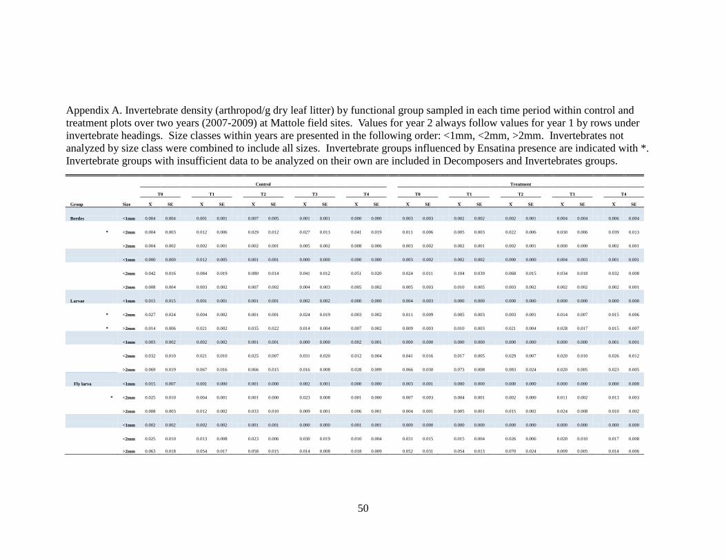
50

Appendix A. Invertebrate density (arthropod/g dry leaf litter) by functional group sampled in each time period within control and

treatment plots over two years (2007-2009) at Mattole field sites. Values for year 2 always follow values for year 1 by rows under

invertebrate headings. Size classes within years are presented in the following order: <1mm, <2mm, >2mm. Invertebrates not

analyzed by size class were combined to include all sizes. Invertebrate groups influenced by Ensatina presence are indicated with *.

Invertebrate groups with insufficient data to be analyzed on their own are included in Decomposers and Invertebrates groups.

Control Treatment

T0

T1

T2

T3

T4

T0

T1

T2

T3

T4

Group Size Χ SE

Χ SE

Χ SE

Χ SE

Χ SE

Χ SE

Χ SE

Χ SE

Χ SE

Χ SE

Beetles <1mm 0.004 0.004 0.001 0.001 0.007 0.005 0.001 0.001 0.000 0.000 0.003 0.003 0.002 0.002 0.002 0.001 0.004 0.004 0.006 0.004

* <2mm 0.004 0.003

0.012 0.006

0.029 0.012

0.027 0.013

0.041 0.019

0.011 0.006

0.005 0.003

0.022 0.006

0.030 0.006

0.039 0.013

>2mm 0.004 0.002

0.002 0.001

0.002 0.001

0.005 0.002

0.008 0.006

0.003 0.002

0.002 0.001

0.002 0.001

0.000 0.000

0.002 0.001

<1mm 0.000 0.000 0.012 0.005 0.001 0.001 0.000 0.000 0.000 0.000 0.003 0.002 0.002 0.002 0.000 0.000 0.004 0.003 0.001 0.001

<2mm 0.042 0.016

0.084 0.019

0.080 0.014

0.041 0.012

0.051 0.020

0.024 0.011

0.104 0.039

0.068 0.015

0.034 0.018

0.032 0.008

>2mm 0.008 0.004

0.003 0.002

0.007 0.002

0.004 0.003

0.005 0.002

0.005 0.003

0.010 0.005

0.003 0.002

0.002 0.002

0.002 0.001

Larvae <1mm 0.015 0.015 0.001 0.001 0.001 0.001 0.002 0.002 0.000 0.000 0.004 0.003 0.000 0.000 0.000 0.000 0.000 0.000 0.000 0.000

* <2mm 0.027 0.024

0.004 0.002

0.001 0.001

0.024 0.019

0.003 0.002

0.011 0.009

0.005 0.003

0.003 0.001

0.014 0.007

0.015 0.006

* >2mm 0.014 0.006

0.021 0.002

0.035 0.022

0.014 0.004

0.007 0.002

0.009 0.003

0.010 0.003

0.021 0.004

0.028 0.017

0.015 0.007

<1mm 0.003 0.002 0.002 0.002 0.001 0.001 0.000 0.000 0.002 0.001 0.000 0.000 0.000 0.000 0.000 0.000 0.000 0.000 0.001 0.001

<2mm 0.032 0.010

0.021 0.010

0.025 0.007

0.031 0.020

0.012 0.004

0.041 0.016

0.017 0.005

0.029 0.007

0.020 0.010

0.026 0.012

>2mm 0.069 0.019

0.067 0.016

0.066 0.015

0.016 0.008

0.028 0.009

0.066 0.030

0.073 0.008

0.083 0.024

0.020 0.005

0.023 0.005

Fly larva <1mm 0.015 0.007 0.001 0.000 0.001 0.000 0.002 0.001 0.000 0.000 0.003 0.001 0.000 0.000 0.000 0.000 0.000 0.000 0.000 0.000

* <2mm 0.025 0.010

0.004 0.001

0.001 0.000

0.023 0.008

0.001 0.000

0.007 0.003

0.004 0.001

0.002 0.000

0.011 0.002

0.013 0.003

>2mm 0.008 0.003

0.012 0.002

0.033 0.010

0.009 0.001

0.006 0.001

0.004 0.001

0.005 0.001

0.015 0.002

0.024 0.008

0.010 0.002

<1mm 0.002 0.002 0.002 0.002 0.001 0.001 0.000 0.000 0.001 0.001 0.000 0.000 0.000 0.000 0.000 0.000 0.000 0.000 0.000 0.000

<2mm 0.025 0.010

0.013 0.008

0.023 0.006

0.030 0.019

0.010 0.004

0.031 0.015

0.015 0.004

0.026 0.006

0.020 0.010

0.017 0.008

>2mm 0.063 0.018

0.054 0.017

0.058 0.015

0.014 0.008

0.018 0.009

0.052 0.031

0.054 0.013

0.070 0.024

0.009 0.005

0.014 0.006

51

Control Treatment

T0

T1

T2

T3

T4

T0

T1

T2

T3

T4

Group Size Χ SE Χ SE Χ SE Χ SE Χ SE Χ SE Χ SE Χ SE Χ SE Χ SE

Beetle Larva <1mm 0.000 0.000 0.001 0.001 0.000 0.000 0.000 0.000 0.000 0.000 0.001 0.001 0.000 0.000 0.000 0.000 0.000 0.000 0.000 0.000

* <2mm 0.002 0.002

0.001 0.001

0.000 0.000

0.001 0.001

0.002 0.001

0.004 0.003

0.001 0.001

0.000 0.000

0.003 0.002

0.002 0.002

* >2mm 0.005 0.001

0.009 0.002

0.002 0.001

0.004 0.002

0.001 0.001

0.006 0.002

0.005 0.002

0.003 0.002

0.004 0.002

0.004 0.003

<1mm 0.000 0.000 0.000 0.000 0.000 0.000 0.000 0.000 0.000 0.000 0.000 0.000 0.000 0.000 0.000 0.000 0.000 0.000 0.000 0.000

* <2mm 0.004 0.002

0.002 0.002

0.001 0.001

0.000 0.000

0.000 0.000

0.011 0.007

0.002 0.002

0.002 0.002

0.000 0.000

0.000 0.000

>2mm 0.005 0.002

0.003 0.002

0.004 0.002

0.000 0.000

0.001 0.001

0.011 0.005

0.012 0.009

0.006 0.004

0.004 0.003

0.003 0.002

Springtails <1mm 0.431 0.296 0.073 0.035 0.073 0.023 0.076 0.045 0.208 0.026 0.473 0.400 0.076 0.028 0.077 0.029 0.162 0.081 0.300 0.082

<2mm 0.099 0.056

0.033 0.006

0.044 0.013

0.057 0.023

0.057 0.010

0.098 0.063

0.034 0.009

0.038 0.011

0.055 0.020

0.103 0.031

>2mm 0.013 0.007

0.005 0.002

0.005 0.003

0.004 0.002

0.002 0.001

0.020 0.013

0.011 0.004

0.008 0.003

0.006 0.004

0.007 0.004

<1mm 0.527 0.121 1.020 0.112 0.578 0.159 0.737 0.369 0.382 0.134 0.466 0.102 0.857 0.301 0.721 0.149 0.509 0.212 0.475 0.066

<2mm 0.252 0.055

0.511 0.071

0.301 0.055

0.188 0.077

0.136 0.054

0.303 0.060

0.437 0.092

0.287 0.068

0.134 0.030

0.165 0.040

>2mm 0.027 0.009

0.038 0.006

0.007 0.002

0.002 0.001

0.000 0.000

0.025 0.008

0.025 0.009

0.013 0.003

0.005 0.003

0.004 0.002

Entomobryidae <1mm 0.011 0.009 0.010 0.007 0.015 0.007 0.012 0.006 0.038 0.015 0.037 0.025 0.019 0.008 0.009 0.003 0.007 0.003 0.030 0.025

* <2mm 0.009 0.008

0.012 0.003

0.012 0.007

0.014 0.003

0.022 0.010

0.019 0.012

0.009 0.002

0.006 0.002

0.020 0.008

0.017 0.009

>2mm 0.006 0.003

0.004 0.002

0.002 0.001

0.002 0.001

0.001 0.001

0.010 0.007

0.006 0.002

0.006 0.003

0.003 0.002

0.003 0.002

<1mm 0.052 0.028 0.106 0.031 0.070 0.015 0.138 0.056 0.122 0.074 0.029 0.011 0.118 0.056 0.081 0.018 0.051 0.016 0.114 0.044

<2mm 0.025 0.010

0.095 0.029

0.087 0.016

0.082 0.044

0.078 0.038

0.028 0.009

0.079 0.029

0.088 0.027

0.064 0.019

0.076 0.026

>2mm 0.013 0.009

0.013 0.005

0.003 0.002

0.002 0.001

0.000 0.000

0.006 0.004

0.014 0.004

0.009 0.002

0.004 0.003

0.004 0.002

Isotomidae <1mm 0.329 0.234 0.058 0.027 0.040 0.015 0.020 0.017 0.057 0.021 0.282 0.244 0.053 0.023 0.059 0.027 0.067 0.044 0.124 0.030

<2mm 0.062 0.033

0.012 0.003

0.016 0.006

0.011 0.010

0.006 0.003

0.025 0.010

0.015 0.006

0.016 0.006

0.012 0.005

0.033 0.009

>2mm 0.004 0.003

0.000 0.000

0.002 0.001

0.001 0.001

0.001 0.001

0.010 0.006

0.003 0.002

0.002 0.001

0.002 0.002

0.004 0.002

<1mm 0.162 0.031 0.661 0.103 0.384 0.128 0.471 0.289 0.120 0.030 0.200 0.065 0.569 0.288 0.465 0.100 0.322 0.151 0.203 0.035

<2mm 0.055 0.007

0.164 0.034

0.108 0.026

0.043 0.023

0.013 0.006

0.065 0.011

0.157 0.043

0.128 0.051

0.024 0.009

0.028 0.009

>2mm 0.008 0.002

0.024 0.006

0.003 0.001

0.000 0.000

0.000 0.000

0.017 0.009

0.007 0.004

0.005 0.003

0.000 0.000

0.000 0.000

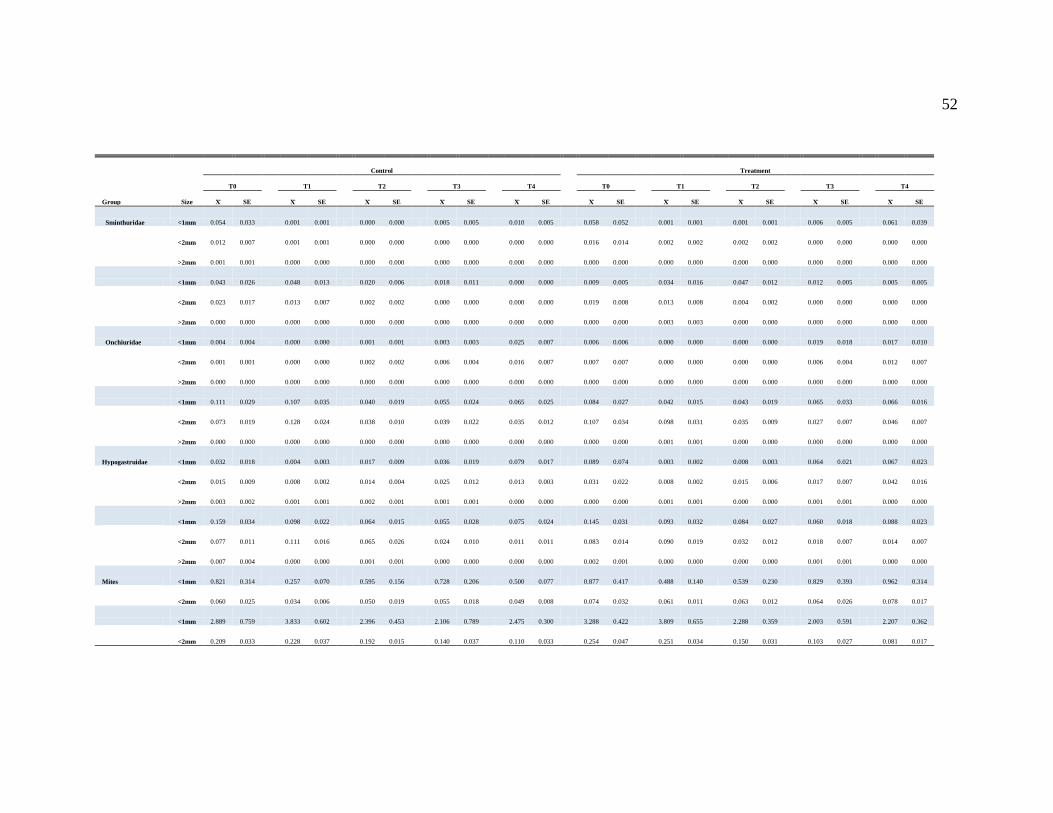
52

Control Treatment

T0

T1

T2

T3

T4

T0

T1

T2

T3

T4

Group Size Χ SE Χ SE Χ SE Χ SE Χ SE Χ SE Χ SE Χ SE Χ SE Χ SE

Sminthuridae <1mm 0.054 0.033 0.001 0.001 0.000 0.000 0.005 0.005 0.010 0.005 0.058 0.052 0.001 0.001 0.001 0.001 0.006 0.005 0.061 0.039

<2mm 0.012 0.007

0.001 0.001

0.000 0.000

0.000 0.000

0.000 0.000

0.016 0.014

0.002 0.002

0.002 0.002

0.000 0.000

0.000 0.000

>2mm 0.001 0.001

0.000 0.000

0.000 0.000

0.000 0.000

0.000 0.000

0.000 0.000

0.000 0.000

0.000 0.000

0.000 0.000

0.000 0.000

<1mm 0.043 0.026 0.048 0.013 0.020 0.006 0.018 0.011 0.000 0.000 0.009 0.005 0.034 0.016 0.047 0.012 0.012 0.005 0.005 0.005

<2mm 0.023 0.017

0.013 0.007

0.002 0.002

0.000 0.000

0.000 0.000

0.019 0.008

0.013 0.008

0.004 0.002

0.000 0.000

0.000 0.000

>2mm 0.000 0.000

0.000 0.000

0.000 0.000

0.000 0.000

0.000 0.000

0.000 0.000

0.003 0.003

0.000 0.000

0.000 0.000

0.000 0.000

Onchiuridae <1mm 0.004 0.004 0.000 0.000 0.001 0.001 0.003 0.003 0.025 0.007 0.006 0.006 0.000 0.000 0.000 0.000 0.019 0.018 0.017 0.010

<2mm 0.001 0.001

0.000 0.000

0.002 0.002

0.006 0.004

0.016 0.007

0.007 0.007

0.000 0.000

0.000 0.000

0.006 0.004

0.012 0.007

>2mm 0.000 0.000

0.000 0.000

0.000 0.000

0.000 0.000

0.000 0.000

0.000 0.000

0.000 0.000

0.000 0.000

0.000 0.000

0.000 0.000

<1mm 0.111 0.029 0.107 0.035 0.040 0.019 0.055 0.024 0.065 0.025 0.084 0.027 0.042 0.015 0.043 0.019 0.065 0.033 0.066 0.016

<2mm 0.073 0.019

0.128 0.024

0.038 0.010

0.039 0.022

0.035 0.012

0.107 0.034

0.098 0.031

0.035 0.009

0.027 0.007

0.046 0.007

>2mm 0.000 0.000

0.000 0.000

0.000 0.000

0.000 0.000

0.000 0.000

0.000 0.000

0.001 0.001

0.000 0.000

0.000 0.000

0.000 0.000

Hypogastruidae <1mm 0.032 0.018 0.004 0.003 0.017 0.009 0.036 0.019 0.079 0.017 0.089 0.074 0.003 0.002 0.008 0.003 0.064 0.021 0.067 0.023

<2mm 0.015 0.009

0.008 0.002

0.014 0.004

0.025 0.012

0.013 0.003

0.031 0.022

0.008 0.002

0.015 0.006

0.017 0.007

0.042 0.016

>2mm 0.003 0.002

0.001 0.001

0.002 0.001

0.001 0.001

0.000 0.000

0.000 0.000

0.001 0.001

0.000 0.000

0.001 0.001

0.000 0.000

<1mm 0.159 0.034 0.098 0.022 0.064 0.015 0.055 0.028 0.075 0.024 0.145 0.031 0.093 0.032 0.084 0.027 0.060 0.018 0.088 0.023

<2mm 0.077 0.011

0.111 0.016

0.065 0.026

0.024 0.010

0.011 0.011

0.083 0.014

0.090 0.019

0.032 0.012

0.018 0.007

0.014 0.007

>2mm 0.007 0.004

0.000 0.000

0.001 0.001

0.000 0.000

0.000 0.000

0.002 0.001

0.000 0.000

0.000 0.000

0.001 0.001

0.000 0.000

Mites <1mm 0.821 0.314 0.257 0.070 0.595 0.156 0.728 0.206 0.500 0.077 0.877 0.417 0.488 0.140 0.539 0.230 0.829 0.393 0.962 0.314

<2mm 0.060 0.025

0.034 0.006

0.050 0.019

0.055 0.018

0.049 0.008

0.074 0.032

0.061 0.011

0.063 0.012

0.064 0.026

0.078 0.017

<1mm 2.889 0.759 3.833 0.602 2.396 0.453 2.106 0.789 2.475 0.300 3.288 0.422 3.809 0.655 2.288 0.359 2.003 0.591 2.207 0.362

<2mm 0.209 0.033

0.228 0.037

0.192 0.015

0.140 0.037

0.110 0.033

0.254 0.047

0.251 0.034

0.150 0.031

0.103 0.027

0.081 0.017

53

Control Treatment

T0

T1

T2

T3

T4

T0

T1

T2

T3

T4

Group Size Χ SE Χ SE Χ SE Χ SE Χ SE Χ SE Χ SE Χ SE Χ SE Χ SE

Orabatidae * <1mm 0.647 0.256 0.178 0.047 0.363 0.107 0.470 0.133 0.339 0.062 0.693 0.331 0.372 0.115 0.314 0.129 0.442 0.224 0.575 0.166

<2mm 0.046 0.022 0.019 0.002 0.027 0.010 0.036 0.012 0.026 0.002 0.048 0.023 0.043 0.012 0.044 0.009 0.046 0.020 0.050 0.014

<1mm 1.870 0.565 2.277 0.307 1.488 0.273 1.303 0.451 1.518 0.202 2.104 0.304 2.226 0.310 1.246 0.203 1.203 0.328 1.237 0.159

<2mm 0.118 0.024 0.125 0.024 0.093 0.010 0.072 0.021 0.037 0.011 0.144 0.041 0.143 0.023 0.076 0.014 0.059 0.015 0.023 0.005

Non-Orabatidae <1mm 0.174 0.059 0.078 0.024 0.232 0.065 0.258 0.076 0.161 0.017 0.184 0.096 0.116 0.031 0.224 0.105 0.387 0.171 0.387 0.159

<2mm 0.015 0.004

0.015 0.006

0.023 0.010

0.019 0.006

0.023 0.007

0.026 0.009

0.018 0.004

0.018 0.004

0.018 0.006

0.028 0.005

<1mm 1.019 0.206 1.557 0.330 0.908 0.206 0.803 0.347 0.958 0.147 1.184 0.139 1.583 0.372 1.042 0.178 0.799 0.277 0.970 0.206

<2mm 0.091 0.013

0.103 0.025

0.098 0.020

0.068 0.019

0.073 0.023

0.110 0.015

0.108 0.018

0.073 0.018

0.044 0.014

0.058 0.015

Milipedes * All 0.006 0.003 0.001 0.001 0.000 0.000 0.005 0.004 0.000 0.000 0.000 0.000 0.003 0.002 0.002 0.002 0.002 0.001 0.019 0.019

All 0.002 0.002

0.004 0.002

0.000 0.000

0.003 0.002

0.004 0.003

0.002 0.002

0.000 0.000

0.003 0.002

0.003 0.001

0.000 0.000

Worms All 0.002 0.002 0.000 0.000 0.001 0.001 0.001 0.001 0.003 0.002 0.007 0.005 0.002 0.002 0.007 0.004 0.002 0.001 0.003 0.002

* All 0.003 0.002

0.015 0.006

0.010 0.004

0.021 0.009

0.006 0.003

0.013 0.008

0.015 0.005

0.021 0.008

0.025 0.013

0.013 0.002

Diplura All 0.020 0.011 0.001 0.001 0.006 0.003 0.004 0.002 0.005 0.004 0.015 0.009 0.002 0.002 0.005 0.001 0.001 0.001 0.012 0.008

All 0.006 0.002

0.009 0.005

0.011 0.004

0.008 0.006

0.016 0.003

0.015 0.005

0.005 0.003

0.020 0.009

0.014 0.002

0.012 0.005

Protura All 0.066 0.037 0.005 0.003 0.024 0.018 0.012 0.005 0.004 0.002 0.047 0.020 0.016 0.007 0.021 0.010 0.014 0.010 0.004 0.002

All 0.039 0.020

0.013 0.006

0.025 0.014

0.036 0.019

0.019 0.012

0.050 0.019

0.017 0.006

0.015 0.006

0.047 0.038

0.026 0.009

Barklice All 0.001 0.001 0.000 0.000 0.000 0.000 0.001 0.001 0.000 0.000 0.002 0.001 0.000 0.000 0.000 0.000 0.001 0.001 0.001 0.001

* All 0.003 0.002

0.008 0.003

0.004 0.002

0.021 0.005

0.012 0.007

0.003 0.002

0.008 0.002

0.007 0.004

0.020 0.008

0.037 0.011

Termites All 0.000 0.000 0.000 0.000 0.000 0.000 0.000 0.000 0.000 0.000 0.000 0.000 0.000 0.000 0.000 0.000 0.000 0.000 0.000 0.000

* All 0.000 0.000

0.000 0.000

0.001 0.001

0.000 0.000

0.000 0.000

0.000 0.000

0.000 0.000

0.000 0.000

0.000 0.000

0.000 0.000

Symphyla All 0.005 0.002 0.000 0.000 0.005 0.003 0.001 0.001 0.003 0.001 0.007 0.002 0.004 0.001 0.006 0.004 0.007 0.004 0.003 0.001

All 0.022 0.005

0.002 0.002

0.005 0.002

0.009 0.005

0.007 0.005

0.013 0.006

0.004 0.003

0.019 0.008

0.011 0.006

0.021 0.010

Earwigs * All 0.000 0.000 0.005 0.002 0.003 0.002 0.002 0.002 0.002 0.001 0.001 0.001 0.002 0.001 0.003 0.001 0.001 0.001 0.000 0.000

All 0.003 0.001

0.000 0.000

0.000 0.000

0.002 0.002

0.006 0.003

0.004 0.004

0.002 0.002

0.001 0.001

0.000 0.000

0.003 0.002

54

Control Treatment

T0

T1

T2

T3

T4

T0

T1

T2

T3

T4

Group Χ SE Χ SE Χ SE Χ SE Χ SE Χ SE Χ SE Χ SE Χ SE Χ SE

Decomposers <1mm 1.324 0.627 0.334 0.102 0.686 0.179 0.787 0.251 0.710 0.062 1.410 0.822 0.574 0.157 0.632 0.259 0.997 0.420 1.270 0.341

<2mm 0.222 0.120 0.087 0.013 0.142 0.048 0.174 0.074 0.155 0.026 0.208 0.095 0.116 0.017 0.135 0.028 0.182 0.064 0.246 0.052

>2mm 0.047 0.018 0.033 0.002 0.051 0.024 0.028 0.007 0.019 0.006 0.043 0.020 0.031 0.004 0.048 0.011 0.039 0.018 0.037 0.013

<1mm 3.435 0.876 4.873 0.675 2.977 0.600 2.880 1.162 2.876 0.407 3.780 0.444 4.672 0.924 3.022 0.500 2.556 0.820 2.709 0.400

<2mm 0.576 0.091 0.870 0.105 0.646 0.064 0.432 0.151 0.343 0.065 0.662 0.084 0.837 0.145 0.575 0.113 0.352 0.085 0.363 0.065

>2mm 0.122 0.027 0.130 0.016 0.090 0.015 0.046 0.019 0.056 0.017 0.130 0.040 0.123 0.002 0.130 0.032 0.050 0.015 0.058 0.014

Predators All 0.040 0.017 0.018 0.002 0.022 0.004 0.030 0.010 0.026 0.010 0.025 0.005 0.025 0.006 0.009 0.003 0.023 0.010 0.024 0.006

All 0.076 0.017

0.092 0.009

0.076 0.009

0.060 0.022

0.082 0.029

0.089 0.019

0.075 0.015

0.055 0.009

0.088 0.029

0.071 0.013

Centipedes All 0.011 0.003 0.007 0.003 0.013 0.002 0.011 0.005 0.009 0.002 0.009 0.004 0.008 0.001 0.004 0.002 0.009 0.004 0.009 0.002

All 0.016 0.003

0.035 0.010

0.033 0.008

0.018 0.006

0.031 0.004

0.032 0.008

0.037 0.011

0.019 0.006

0.031 0.010

0.026 0.007

Pseudoscrpions All 0.007 0.003 0.002 0.002 0.002 0.002 0.006 0.004 0.001 0.001 0.004 0.002 0.006 0.005 0.002 0.001 0.002 0.002 0.004 0.002

* All 0.009 0.005

0.004 0.002

0.008 0.003

0.004 0.002

0.006 0.004

0.006 0.002

0.009 0.002

0.007 0.003

0.005 0.003

0.010 0.003

Predatory larva <1mm 0.000 0.000 0.000 0.000 0.000 0.000 0.000 0.000 0.000 0.000 0.000 0.000 0.000 0.000 0.000 0.000 0.000 0.000 0.000 0.000

<2mm 0.002 0.002

0.000 0.000

0.000 0.000

0.001 0.001

0.000 0.000

0.001 0.001

0.000 0.000

0.000 0.000

0.003 0.002

0.000 0.000

>2mm 0.003 0.002

0.004 0.001

0.003 0.002

0.005 0.002

0.001 0.001

0.003 0.001

0.004 0.002

0.001 0.001

0.002 0.001

0.003 0.002

<1mm 0.000 0.000 0.000 0.000 0.000 0.000 0.001 0.001 0.000 0.000 0.000 0.000 0.000 0.000 0.000 0.000 0.000 0.000 0.000 0.000

<2mm 0.007 0.003

0.012 0.004

0.003 0.002

0.005 0.003

0.006 0.004

0.011 0.003

0.002 0.002

0.003 0.002

0.005 0.002

0.010 0.006

>2mm 0.012 0.006

0.012 0.003

0.009 0.005

0.013 0.006

0.006 0.002

0.013 0.006

0.007 0.003

0.005 0.002

0.014 0.009

0.011 0.005

Spiders <1mm 0.008 0.008 0.000 0.000 0.001 0.001 0.002 0.001 0.000 0.000 0.001 0.001 0.001 0.001 0.000 0.000 0.000 0.000 0.000 0.000

* <2mm 0.002 0.002

0.001 0.001

0.001 0.001

0.000 0.000

0.003 0.001

0.003 0.001

0.001 0.002

0.001 0.001

0.004 0.001

0.004 0.002

>2mm 0.003 0.003

0.002 0.001

0.001 0.001

0.001 0.001

0.004 0.003

0.003 0.002

0.001 0.001

0.000 0.000

0.001 0.001

0.004 0.002

<1mm 0.000 0.000 0.000 0.000 0.001 0.001 0.000 0.000 0.000 0.000 0.000 0.000 0.002 0.002 0.001 0.001 0.000 0.000 0.002 0.002

<2mm 0.019 0.005

0.015 0.004

0.012 0.003

0.012 0.007

0.023 0.014

0.012 0.005

0.008 0.003

0.012 0.001

0.019 0.007

0.005 0.003

>2mm 0.001 0.001

0.013 0.006

0.003 0.001

0.001 0.001

0.004 0.002

0.009 0.005

0.001 0.001

0.002 0.001

0.007 0.002

0.004 0.002

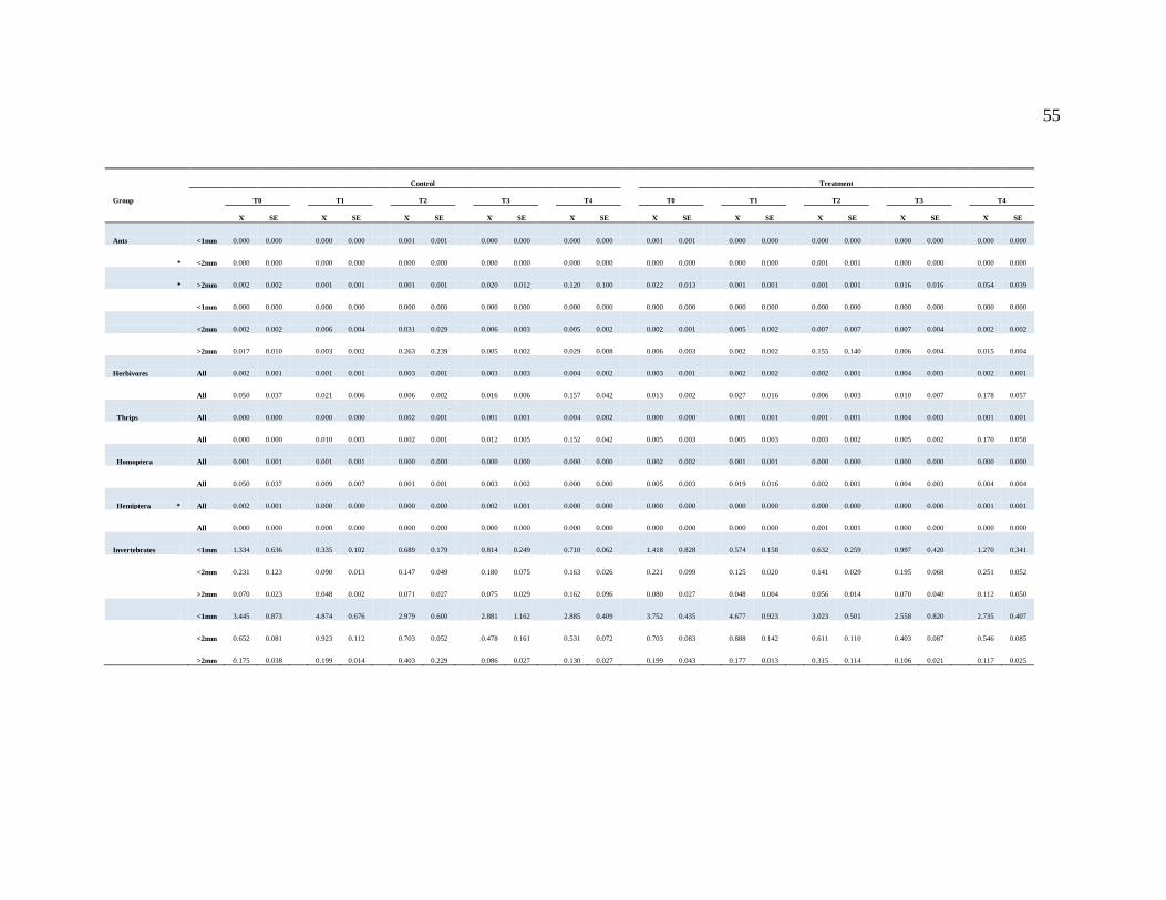
55

Control Treatment

Group

T0

T1

T2

T3

T4

T0

T1

T2

T3

T4

Χ SE Χ SE Χ SE Χ SE Χ SE Χ SE Χ SE Χ SE Χ SE Χ SE

Ants <1mm 0.000 0.000 0.000 0.000 0.001 0.001 0.000 0.000 0.000 0.000 0.001 0.001 0.000 0.000 0.000 0.000 0.000 0.000 0.000 0.000

* <2mm 0.000 0.000 0.000 0.000 0.000 0.000 0.000 0.000 0.000 0.000 0.000 0.000 0.000 0.000 0.001 0.001 0.000 0.000 0.000 0.000

* >2mm 0.002 0.002 0.001 0.001 0.001 0.001 0.020 0.012 0.120 0.100 0.022 0.013 0.001 0.001 0.001 0.001 0.016 0.016 0.054 0.039

<1mm 0.000 0.000 0.000 0.000 0.000 0.000 0.000 0.000 0.000 0.000 0.000 0.000 0.000 0.000 0.000 0.000 0.000 0.000 0.000 0.000

<2mm 0.002 0.002 0.006 0.004 0.031 0.029 0.006 0.003 0.005 0.002 0.002 0.001 0.005 0.002 0.007 0.007 0.007 0.004 0.002 0.002

>2mm 0.017 0.010 0.003 0.002 0.263 0.239 0.005 0.002 0.029 0.008 0.006 0.003 0.002 0.002 0.155 0.140 0.006 0.004 0.015 0.004

Herbivores All 0.002 0.001 0.001 0.001 0.003 0.001 0.003 0.003 0.004 0.002 0.003 0.001 0.002 0.002 0.002 0.001 0.004 0.003 0.002 0.001

All 0.050 0.037 0.021 0.006 0.006 0.002 0.016 0.006 0.157 0.042 0.013 0.002 0.027 0.016 0.006 0.003 0.010 0.007 0.178 0.057

Thrips All 0.000 0.000 0.000 0.000 0.002 0.001 0.001 0.001 0.004 0.002 0.000 0.000 0.001 0.001 0.001 0.001 0.004 0.003 0.001 0.001

All 0.000 0.000

0.010 0.003

0.002 0.001

0.012 0.005

0.152 0.042

0.005 0.003

0.005 0.003

0.003 0.002

0.005 0.002

0.170 0.058

Homoptera All 0.001 0.001 0.001 0.001 0.000 0.000 0.000 0.000 0.000 0.000 0.002 0.002 0.001 0.001 0.000 0.000 0.000 0.000 0.000 0.000

All 0.050 0.037

0.009 0.007

0.001 0.001

0.003 0.002

0.000 0.000

0.005 0.003

0.019 0.016

0.002 0.001

0.004 0.003

0.004 0.004

Hemiptera * All 0.002 0.001 0.000 0.000 0.000 0.000 0.002 0.001 0.000 0.000 0.000 0.000 0.000 0.000 0.000 0.000 0.000 0.000 0.001 0.001

All 0.000 0.000

0.000 0.000

0.000 0.000

0.000 0.000

0.000 0.000

0.000 0.000

0.000 0.000

0.001 0.001

0.000 0.000

0.000 0.000

Invertebrates <1mm 1.334 0.636 0.335 0.102 0.689 0.179 0.814 0.249 0.710 0.062 1.418 0.828 0.574 0.158 0.632 0.259 0.997 0.420 1.270 0.341

<2mm 0.231 0.123

0.090 0.013

0.147 0.049

0.180 0.075

0.163 0.026

0.221 0.099

0.125 0.020

0.141 0.029

0.195 0.068

0.251 0.052

>2mm 0.070 0.023

0.048 0.002

0.071 0.027

0.075 0.029

0.162 0.096

0.080 0.027

0.048 0.004

0.056 0.014

0.070 0.040

0.112 0.050

<1mm 3.445 0.873 4.874 0.676 2.979 0.600 2.881 1.162 2.885 0.409 3.752 0.435 4.677 0.923 3.023 0.501 2.558 0.820 2.735 0.407

<2mm 0.652 0.081

0.923 0.112

0.703 0.052

0.478 0.161

0.531 0.072

0.703 0.083

0.888 0.142

0.611 0.110

0.403 0.087

0.546 0.085

>2mm 0.175 0.038 0.199 0.014 0.403 0.229 0.086 0.027 0.130 0.027 0.199 0.043 0.177 0.013 0.315 0.114 0.106 0.021 0.117 0.025