Ecological Management Decision Support System...

EMDS Appendix NCWAP STAFF

1

Ecological Management Decision Support System (EMDS) I. Ecological Management Decision Support (EMDS): A NCWAP Tool for Data Synthesis and Analysis

Introduction NCWAP has selected the Ecological Management Decision Support (EMDS) (Reynolds 1999) software to help evaluate and synthesize information on watershed and stream conditions important to salmonids during the freshwater phases of their life history (Note: we are excluding factors related to marine habitat and fishing). EMDS uses linguistically based models, which are frequently utilized in engineering and the applied sciences to formalize expert opinion. The approach is one of several that NCWAP is employing to aid in identifying habitat factors that affect the production of salmonids on California’s North Coast Watersheds (see limiting factors discussion in the Synthesis Report). The EMDS appendix describes the general workings of EMDS and the details of the models NCWAP is developing in conjunction with it . NCWAP scientists have constructed “knowledge base” models to identify and evaluate environmental factors (e.g., watershed geology, stream sediment loading, stream temperature, land use activities, etc.) which taken together shape anadromous salmonid habitat. Based upon these models, EMDS evaluates available data to provide insight into the conditions of the streams and watersheds for salmonids in the region. The synthesis EMDS provides can then be compared to more direct measures of salmonid production—i.e., the number of salmonids recently found in streams. EMDS offers a number of benefits for the assessment work that NCWAP is conducting, and also has some known limitations. Both the advantages and drawbacks of EMDS are provided in some detail in this appendix. Our use of the EMDS model outputs in this report is tentative. As discussed below, a scientific peer review process conducted in April of 2002 indicated that substantial changes to NCWAP’s EMDS modeling approach are needed. At the time of the production of this report, we have been able to implement some, but not all of these recommendations. Hence, we use the model outputs with caution at this time. NCWAP will continue to work to refine and improve the EMDS model, based on the peer review.

Background Details of the EMDS Software EMDS (Reynolds 1999), was recently developed by Dr. Keith Reynolds at the USDA-Forest Service, Pacific Northwest Research Station. It employs a linked set of software that includes MS Excel, NetWeaver, the Ecological Management Decision Support (EMDS) ArcView Extension, and ArcView™. Microsoft Excel is a commonly used spreadsheet program for data storage and analysis. NetWeaver (Saunders and Miller (no date)),


2

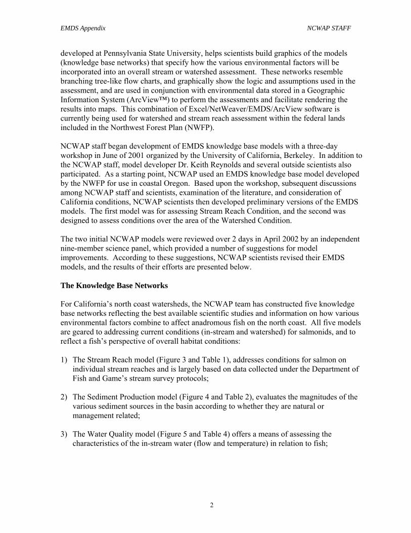
developed at Pennsylvania State University, helps scientists build graphics of the models (knowledge base networks) that specify how the various environmental factors will be incorporated into an overall stream or watershed assessment. These networks resemble branching tree-like flow charts, and graphically show the logic and assumptions used in the assessment, and are used in conjunction with environmental data stored in a Geographic Information System (ArcView™) to perform the assessments and facilitate rendering the results into maps. This combination of Excel/NetWeaver/EMDS/ArcView software is currently being used for watershed and stream reach assessment within the federal lands included in the Northwest Forest Plan (NWFP). NCWAP staff began development of EMDS knowledge base models with a three-day workshop in June of 2001 organized by the University of California, Berkeley. In addition to the NCWAP staff, model developer Dr. Keith Reynolds and several outside scientists also participated. As a starting point, NCWAP used an EMDS knowledge base model developed by the NWFP for use in coastal Oregon. Based upon the workshop, subsequent discussions among NCWAP staff and scientists, examination of the literature, and consideration of California conditions, NCWAP scientists then developed preliminary versions of the EMDS models. The first model was for assessing Stream Reach Condition, and the second was designed to assess conditions over the area of the Watershed Condition. The two initial NCWAP models were reviewed over 2 days in April 2002 by an independent nine-member science panel, which provided a number of suggestions for model improvements. According to these suggestions, NCWAP scientists revised their EMDS models, and the results of their efforts are presented below. The Knowledge Base Networks For California’s north coast watersheds, the NCWAP team has constructed five knowledge base networks reflecting the best available scientific studies and information on how various environmental factors combine to affect anadromous fish on the north coast. All five models are geared to addressing current conditions (in-stream and watershed) for salmonids, and to reflect a fish’s perspective of overall habitat conditions: 1) The Stream Reach model (Figure 3 and Table 1), addresses conditions for salmon on

individual stream reaches and is largely based on data collected under the Department of Fish and Game’s stream survey protocols;

2) The Sediment Production model (Figure 4 and Table 2), evaluates the magnitudes of the

various sediment sources in the basin according to whether they are natural or management related;

3) The Water Quality model (Figure 5 and Table 4) offers a means of assessing the

characteristics of the in-stream water (flow and temperature) in relation to fish;


3

4) The Fish Habitat Quality model (Figure 5 and Table 3) incorporates the Stream Reach model results in combination with data on accessibility to spawning fish and a synoptic view of the condition of riparian vegetation for shade and large woody debris;

5) The Fish Food Availability model (Figure 5) has not yet been constructed, but will

evaluate the watershed based upon conditions for producing food sources for anadromous salmonids.

Figure 1 shows the NCWAP EMDS model parameters in relation to work done by Ziemer and Reid (1997). Figure 1 is a re-working of the figure out of their 1997 paper, called “The Shape of the Problem”. The original figure was used by the authors to show the complex linkages among natural and human-related phenomena which combine to affect salmonids in freshwater streams. Here it is redrawn to show more of the flow of various factors (from top to bottom) and with annotation of the parameters that are included in our EMDS models. Graphics such as these help to conceptualize the interrelationships of the problems facing salmonids, and serve as a basis for work such as with building EMDS models to reflect the complex system. In creating the EMDS models listed above, NCWAP scientists have used what is termed a “top-down” approach. This approach is perhaps best explained by way of example. The NCWAP Stream Reach Condition model began with the proposition: The overall condition of the stream reach is suitable for maintaining healthy populations of native coho and chinook salmon, and steelhead trout. A knowledge base (network) model was then designed to evaluate the “truth” of that proposition, based upon data from each stream reach. The model design and contents reflect the specific information NCWAP scientists believed are needed, and the manner in which it should be combined, to test the proposition. In evaluating stream reach conditions for salmonids, the NCWAP model uses data on several environmental factors. The first branching of the knowledge base network (Figure 2) shows that information on in-channel condition, stream flow, riparian vegetation and water temperature are all used as inputs in the stream reach condition model. In turn, each of the four branches is progressively broken into more basic data components that contribute to it (not shown). The process is repeated until the knowledge base network incorporates all information believed to be important to the evaluation. Although model construction is typically done top-down, models are run in EMDS from the “bottom up”. That is, data on the stream reach is usually entered at the lowest branches of the network tree (the “leaves”), and then is combined progressively with other information as it proceeds up the network. Decision nodes are intersections in the model networks where two or more factors are combined before passing the resultant information on up the network. For example, the “AND” at the decision node in Figure 2 means that the lowest value of the four general factors coming in to the model at that point is taken to indicate the potential of the stream reach to sustain salmon populations. EMDS models assess the degree of truth (or falsehood) of each model proposition. Each proposition is evaluated in reference to simple graphs called “reference curves” that


4

Figure 1. Modified from Figure 1 of Ziemer and Reid (1997) “The Shape of the Problem” to show the relationship between EMDS model parameters and the conceptual diagram of problems facing salmon in north coast California freshwater streams. Abbreviations used for watershed models above are: PSP – Potential Sediment Production model; FHQ – Fish Habitat Quality model; WQ – Water Quality model.


5

Figure 2. EMDS Stream Reach Knowledge Base Network. EMDS uses knowledge base networks to assess the condition of watershed factors affecting native salmonids.

determine its degree of truth/falsehood, according to the data’s implications for salmon. Figure 6 shows an example reference curve for the proposition is “the stream temperature is suitable for salmon”. The horizontal axis shows temperature in degrees Fahrenheit, while the vertical is labeled “Truth Value” and ranges from –1 to +1. The line shows what are fully unsuitable temperatures (-1), fully suitable temperatures (+1) and those that are in-between (> -1 and <+1). In this way, a similar numeric relationship is required for all propositions evaluated in the EMDS models. Proposition evaluations do not always result in simple “true” vs. “false” assessments – a strength of EMDS is its capability to determine degrees of truth or falsehood, or in effect, the degree to which the proposition is supported in the model by the evidence. For each evaluated propositions in the network, the result is a number between –1 and +1. The number relates to the degree to which the data support or refute the proposition. In all cases a value of +1 means that the proposition is “completely true”, and –1 implies that it is “completely false”, with in-between values indicate “degrees of truth” (i.e., values approaching +1 being closer to true and those approaching –1 converging on completely untrue). A zero value means that the proposition cannot be evaluated based upon the data available. Breakpoints (where the slope of the reference curve changes) in the Figure 6 example occur at 45, 50, 60 and 68 degrees Fahrenheit. For the Stream Reach model, NCWAP fisheries biologists determined these temperatures by a review of the scientific literature.

For many NCWAP parameters, particularly those relating to upland geology and management activities, effectively no scientific literature is available to assist in determining breakpoints. Because of this, NCWAP has had little alternative but to use a more empirically-based approach for breakpoints. Specifically, for each evaluated parameter, the mean and standard deviation are computed for all planning watersheds in a basin. Breakpoints are then selected to rank each planning watershed for that parameter in relation to all others in the basin. We used a simple linear approximation of the standardized cumulative distribution function, with the 10th and 90th percentiles serving as the low and high breakpoints (Figure 7). Thus the truth values for all Potential Sediment Production model variables are relative measures directly related to the percentile rank of that planning watershed. While not comparable outside of the context of the basin, such rankings do provide an indication of relative conditions within the basin.


6

Figure 3. NCWAP EMDS Anadromous Reach Condition Model.


7

Figure 4. NCWAP EMDS Potential Sediment Production Model.


8

Figure 5. NCWAP EMDS Fish Food Availability, Water Quality and Fish Habitat Quality Models. Note: None of these models has yet been implemented. This graphic shows their current states of development.


9

Maximum Weekly Average Temperature

-1

0

1

30 40 50 60 70 80

water temperature (degrees F)

trut

h va

lue

68

6050

45

Figure 6. EMDS Reference Curve. EMDS uses this type of reference curve in conjunction with data specific to a stream reach. This example curve evaluates the proposition that the stream’s water temperature is suitable for salmonids. Break points can be set for specific species, life stage, or season of the year. Curves are dependent upon the availability of data.

Normalized Cumulative Distribution Function

0

1

-3 -2 -1 0 1 2 3

standard deviations from the mean (0)

cum

ulat

ive

perc

ent

linear approximationof cdf function

line intersectsy=1 at ~ x = 1.3(90th percentile)line intersects

y=0 at ~ x = -1.3(10th percentile)

Figure 7. Using the 10th and 90th percentiles as breakpoints (as with Land Use) is a linear approximation of the central part of the normalized cumulative distribution function

The science review panel recommended that this method developed by NCWAP scientists be changed. They advised to use a set of reference watersheds from the region, compute the distributions of land use and other parameters from those watersheds to determine breakpoints. At this point NCWAP staff have not had the resources to select the reference watersheds, nor to process the data for them. This issue will be addressed in future watershed assessment and the breakpoints adjusted as the information from reference watersheds becomes available.


10

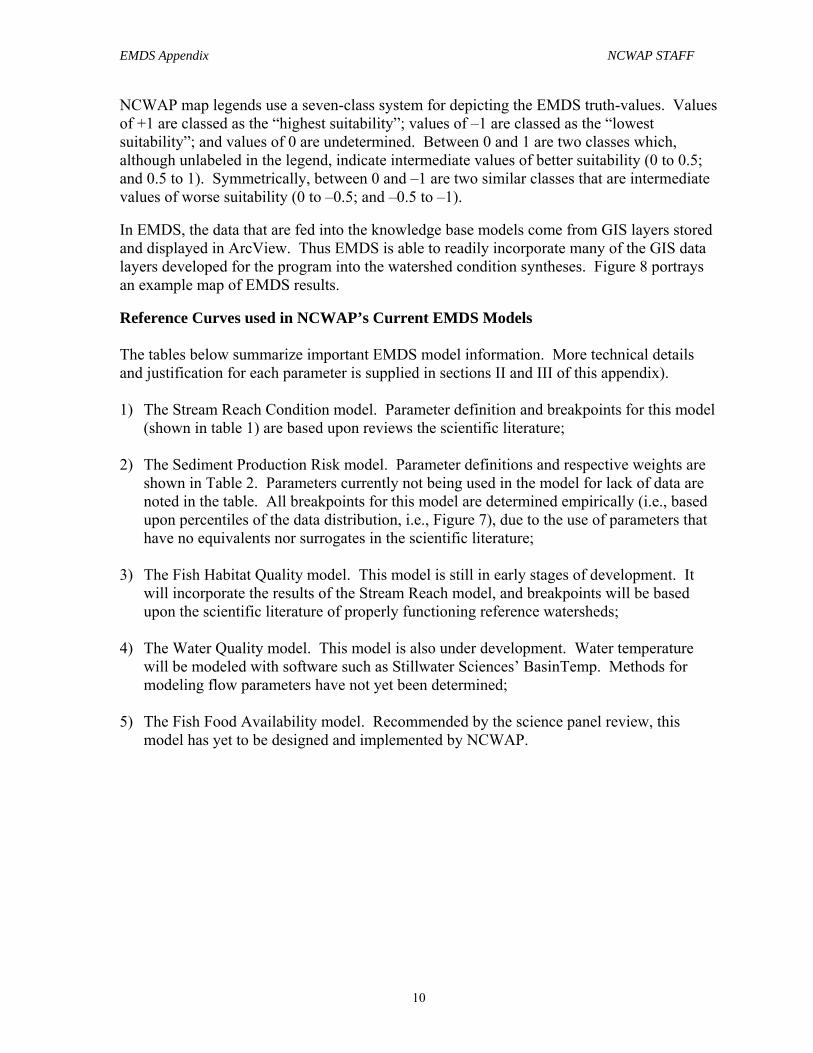
NCWAP map legends use a seven-class system for depicting the EMDS truth-values. Values of +1 are classed as the “highest suitability”; values of –1 are classed as the “lowest suitability”; and values of 0 are undetermined. Between 0 and 1 are two classes which, although unlabeled in the legend, indicate intermediate values of better suitability (0 to 0.5; and 0.5 to 1). Symmetrically, between 0 and –1 are two similar classes that are intermediate values of worse suitability (0 to –0.5; and –0.5 to –1).

In EMDS, the data that are fed into the knowledge base models come from GIS layers stored and displayed in ArcView. Thus EMDS is able to readily incorporate many of the GIS data layers developed for the program into the watershed condition syntheses. Figure 8 portrays an example map of EMDS results.

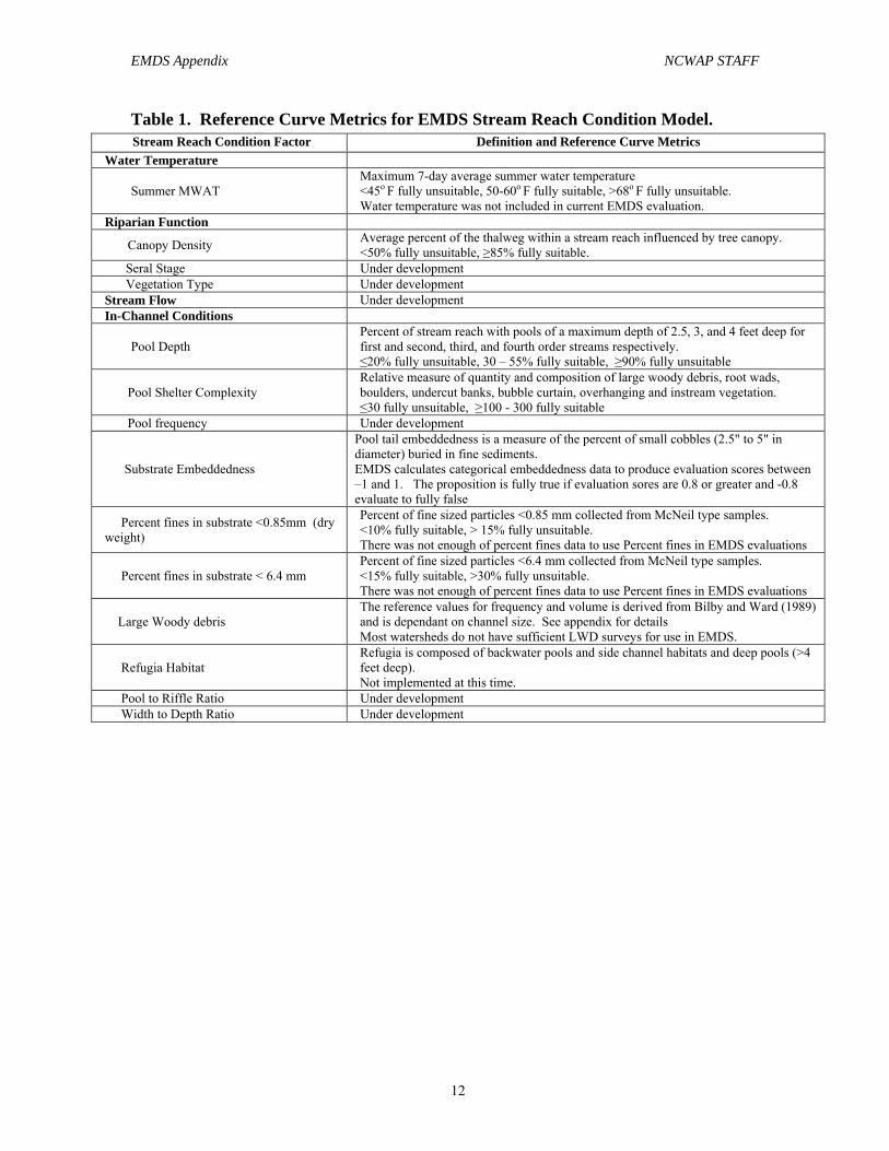
Reference Curves used in NCWAP’s Current EMDS Models The tables below summarize important EMDS model information. More technical details and justification for each parameter is supplied in sections II and III of this appendix). 1) The Stream Reach Condition model. Parameter definition and breakpoints for this model

(shown in table 1) are based upon reviews the scientific literature; 2) The Sediment Production Risk model. Parameter definitions and respective weights are

shown in Table 2. Parameters currently not being used in the model for lack of data are noted in the table. All breakpoints for this model are determined empirically (i.e., based upon percentiles of the data distribution, i.e., Figure 7), due to the use of parameters that have no equivalents nor surrogates in the scientific literature;

3) The Fish Habitat Quality model. This model is still in early stages of development. It

will incorporate the results of the Stream Reach model, and breakpoints will be based upon the scientific literature of properly functioning reference watersheds;

4) The Water Quality model. This model is also under development. Water temperature

will be modeled with software such as Stillwater Sciences’ BasinTemp. Methods for modeling flow parameters have not yet been determined;

5) The Fish Food Availability model. Recommended by the science panel review, this

model has yet to be designed and implemented by NCWAP.


11

Figure 8. EMDS Graphical Output. This example illustrates the graphical outputs of an EMDS run. This demonstration graphic portrays the relative amounts of potential sediment production in the Gualala River Basin that comes from natural sources.


12

Table 1. Reference Curve Metrics for EMDS Stream Reach Condition Model. Stream Reach Condition Factor Definition and Reference Curve Metrics

Water Temperature

Summer MWAT Maximum 7-day average summer water temperature <45o F fully unsuitable, 50-60o F fully suitable, >68o F fully unsuitable. Water temperature was not included in current EMDS evaluation.

Riparian Function

Canopy Density Average percent of the thalweg within a stream reach influenced by tree canopy. <50% fully unsuitable, ≥85% fully suitable.

Seral Stage Under development Vegetation Type Under development Stream Flow Under development In-Channel Conditions

Pool Depth Percent of stream reach with pools of a maximum depth of 2.5, 3, and 4 feet deep for first and second, third, and fourth order streams respectively. ≤20% fully unsuitable, 30 – 55% fully suitable, ≥90% fully unsuitable

Pool Shelter Complexity Relative measure of quantity and composition of large woody debris, root wads, boulders, undercut banks, bubble curtain, overhanging and instream vegetation. ≤30 fully unsuitable, ≥100 - 300 fully suitable

Pool frequency Under development

Substrate Embeddedness

Pool tail embeddedness is a measure of the percent of small cobbles (2.5" to 5" in diameter) buried in fine sediments. EMDS calculates categorical embeddedness data to produce evaluation scores between –1 and 1. The proposition is fully true if evaluation sores are 0.8 or greater and -0.8 evaluate to fully false

Percent fines in substrate <0.85mm (dry weight)

Percent of fine sized particles <0.85 mm collected from McNeil type samples. <10% fully suitable, > 15% fully unsuitable. There was not enough of percent fines data to use Percent fines in EMDS evaluations

Percent fines in substrate < 6.4 mm Percent of fine sized particles <6.4 mm collected from McNeil type samples. <15% fully suitable, >30% fully unsuitable. There was not enough of percent fines data to use Percent fines in EMDS evaluations

Large Woody debris The reference values for frequency and volume is derived from Bilby and Ward (1989) and is dependant on channel size. See appendix for details Most watersheds do not have sufficient LWD surveys for use in EMDS.

Refugia Habitat Refugia is composed of backwater pools and side channel habitats and deep pools (>4 feet deep). Not implemented at this time.

Pool to Riffle Ratio Under development Width to Depth Ratio Under development


13

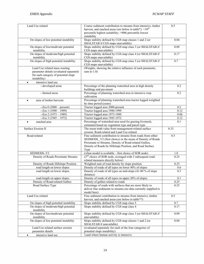
Table 2. Reference Curve Metrics for EMDS Sediment Production Risk Model, version 1.0 Sediment Production Factor Definition* Weights**

Total Sediment Production The mean truth value from Natural Processes and Management-related Processes

Natural Processes The mean truth value from Mass Wasting I, Surface Erosion I and Streamside Erosion I knowledge base networks

0.5

Mass Wasting I The mean truth value from natural mass wasting: Landslide Potential, Deep-seated Landslides and Earth Flows

0.33

Landslide Potential A selective OR (SOR) node takes the best available data to determine landslide mass wasting potential.

1.0

CGS Landslide Potential Map (1st choice of SOR node) Percentage area of planning watershed in the landslide potential categories (4 and 5)

1.0

Landslide Potential Class 5 Percentage area of watershed in class 5 (CGS rating) 0.8 Landslide Potential Class 4 Percentage area of watershed in class 4 (CGS rating) 0.2 Probabilistic Landslide Model (2nd choice of SOR node) Where option 1 is missing, the

Probabilistic Landslide Model is used to calculate area of planning watershed with unstable slopes

1.0

SHALSTAB (3rd choice of SOR node) Where options 1 and 2 are missing, SHALSTAB model is used to calculate area of planning watershed with unstable slopes

1.0

Surface Erosion I The mean truth value from natural processes of surface erosion: Gullies, Soil Creep, and Fires

0.33

Gullies Density of natural gullies in planning watershed (currently no data supplied to model here)

0.33

Soil Creep Percentage area of planning watershed with soil creep (currently no data supplied to model here)

0.33

Fires Percentage area of planning watershed with high fire potential (currently no data supplied to model here)

0.33

Streamside Erosion I The mean truth value from natural processes of streamside erosion: Active Landslides Connected to Watercourses; Active Landslides Not Connected to Watercourses; Disrupted Ground Near Watercourses

0.33

Active Landslides Connected to Watercourses

Percentage of planning watershed with Active Landslides connected to watercourses

0.60

Active Landslides Not Connected to Watercourses

Percentage of planning watershed with Active Landslides not connected to watercourses

0.30

Disrupted Ground near Watercourses Percentage of planning watershed with Disrupted Ground near to watercourses

0.10

Management-related Processes The mean truth value from Mass Wasting II, Surface Erosion II and Streamside Erosion II knowledge base networks

0.5

Mass Wasting II The mean truth value from management-related mass wasting: Road-related and Land Use-related

0.33

Road-related Coarse sediment contribution to streams from roads from either SEDMODL_V2 (first choice) or the mean of Density of Road/Stream Crossing, Density of Roads by Hillslope Position, and Density of Roads on Unstable Slopes

0.5

SEDMODL-V2 (when model is available – 1st choice of SOR node) 1.0 Density of Road/Stream Crossings (2nd choice of SOR node, averaged with DRHP directly below)

Number of road crossings/km of streams 0.33

Density of Roads / Hillslope Position Weighted sum of road density by slope position (weights determine relative influence, and sum to 1.0)

0.33

road length on lower slopes Density of roads of all types on lower 40% of slopes 0.6 road length on lower slopes Density of roads of all types on mid-slope (41-80 % of slope

distance) 0.3

road length on upper slopes Density of roads of all types on upper 20% of slopes 0.1 Density of Roads on Unstable Slopes Density of roads on geologically unstable slopes 0.33


14

Land Use related Coarse sediment contribution to streams from intensive, timber harvest, and ranched areas (see below in table*) <10th percentile highest suitability; >90th percentile lowest suitability

0.5

On slopes of low potential instability Slope stability defined by CGS map classes 1 and 2 (or SHALSTAB if CGS maps unavailable)

0.04

On slopes of low/moderate potential instability

Slope stability defined by CGS map class 3 (or SHALSTAB if CGS maps unavailable)

0.09

On slopes of moderate/high potential instability

Slope stability defined by CGS map class 4 (or SHALSTAB if CGS maps unavailable)

0.17

On slopes of high potential instability Slope stability defined by CGS map class 5 (or SHALSTAB if CGS maps unavailable)

0.7

Land Use related mass wasting parameter details (evaluated separately for each category of potential slope instability)

(Weights, showing the relative influence of each parameter, sum to 1.0)

• intensive land use --developed areas Percentage of the planning watershed area in high density

buildings and pavement 0.2

--farmed areas Percentage of planning watershed area in intensive crop cultivation

0.2

• area of timber harvests Percentage of planning watershed area tractor logged weighted by time period (years)

--Era 0 (2000 – present) Tractor logged area 2000-present 0.2 --Era 1 (1990 – 1999) Tractor logged area 1990-1999 0.12 --Era 2 (1973 – 1989) Tractor logged area 1973-1989 0.06 --Era 3 (1945 – 1972) Tractor logged area 1945-1972 0.12 • ranched area Percentage of watershed area used for grazing livestock;

estimated based on vegetation type and parcel type 0.1

Surface Erosion II The mean truth value from management-related surface erosion: Road-related and Land Use-related

0.33

Road-related Fine sediment contribution to streams from roads from either SEDMODL_V2 (first choice) or the mean of Density of Roads Proximate to Streams, Density of Road-related Gullies, Density of Roads by Hillslope Position, and Road Surface Type

0.5

SEDMODL-V2 (when model is available – first choice of SOR node) 1.0 Density of Roads Proximate Streams (2nd choice of SOR node, averaged with 3 subsequent road-

related measures directly below) 0.25

Density of Roads Hillslope Position Weighted sum of road density by slope position 0.25 road length on lower slopes Density of roads of all types on lower 40% of slopes 0.6 road length on lower slopes Density of roads of all types on mid-slope (41-80 % of slope

distance) 0.3

road length on upper slopes Density of roads of all types on upper 20% of slopes 0.1 Density of Road-related Gullies Density of gullies related to roads 0.25 Road Surface Type Percentage of roads with surfaces that are more likely to

deliver fine sediments to streams (no data currently supplied to model here)

0.25

Land Use related Fine sediment contribution to streams from intensive, timber harvest, and ranched areas (see below in table**)

0.5

On slopes of high potential instability Slope stability defined by CGS map class 5 0.7 On slopes of moderate/high potential instability

Slope stability defined by CGS map class 4 0.17

On slopes of low/moderate potential instability

Slope stability defined by CGS map class 3 (or SHALSTAB if unavailable)

0.09

On slopes of low potential instability Slope stability defined by CGS map classes 1 and 2 (or SHALSTAB if unavailable)

0.04

Land Use related surface erosion parameter details

(evaluated separately for each of the four categories of potential slope instability)

• intensive land use Land where human activity is intensive


15

--developed areas Percentage of the planning watershed area in high density buildings and pavement

0.2

--farmed areas Percentage of planning watershed area in intensive crop cultivation

0.2

• area of timber harvests Percentage of planning watershed area tractor logged, by time period

--Era 0 (2000 – present) Tractor logged area 2000-present 0.3 --Era 1 (1990 – 1999) Tractor logged area 1990-1999 0.2 • ranched area Percentage of planning watershed area used for grazing

livestock; estimated based on vegetation type and parcel type 0.1

Streamside Erosion II The mean truth value from management-related streamside erosion: Road-related and Land Use-related

0.33

Density of Roads Proximate to Streams Length of all roads within 200’ of stream ÷ length of all streams

0.33

Density of Road/Stream Crossings Number of road crossings/km of streams 0.33 Density of In-stream Timber Harvest Landings

Number of legacy timber harvest landings in-stream per unit length of stream

0.33

*all breakpoints for the sediment production risk model were created from the tails of the cumulative distribution function curves for each parameter, at the 10th and 90th percentiles. Thus all resultant values are relative to the basin as a whole, but are not rated on an absolute basis **weights for parameters at each node sum to 1.0; indentation of weight shows the tier where it is summed

Table 3. Reference Curve Metrics for EMDS Fish Habitat Quality Model, version 1.0 (not yet implemented)

Fish Habitat Quality Factor Reference Curve Metric In-Stream Access to Ocean Percentage of historically accessible streams currently accessible to anadromous fish;

<10th percentile highest suitability; >90th percentile lowest suitability Stream Reach Condition model results Input from EMDS Reach Condition Model (see table 1 above).

Riparian Canopy Percent area of riparian vegetation within 200’ feet of stream and compared to canopy closure on reference streams; <10th percentile lowest suitability; >90th percentile highest suitability

Large Woody Debris Potential Large Woody Debris Potential Model 1st choice for SOR node, model not yet identified Large Woody Debris Potential 2nd choice for SOR node. Percentage of stream bordered by mature forest stands. with

quadratic mean diameter of >=24 inches as compared to reference streams; <10th percentile lowest suitability; >90th percentile highest suitability

1st and 2nd order streams 3rd and 4th order streams 5th and 6th order streams

Advantages Offered by EMDS EMDS offers a number of advantages for use by NCWAP. Instead of being a hidden “black box”, each EMDS model has an open and intuitively understandable structure. The explicit nature of the model networks facilitates open communication among agency personnel and with the general public through simple graphics and easily understood flow diagrams. The models can be easily modified to incorporate alternative assumptions about the conditions of specific environmental factors (e.g., stream water temperature) required for suitable salmonid habitat.


16

Using ESRI Geographic Information System (GIS) software, EMDS maps the factors affecting fish habitat and shows how they vary across a basin. At this time no other widely available package allows a knowledge base network to be linked directly with a geographic information system such as ESRI’s ArcView. This link is vital to the production of maps and other graphics reporting the watershed assessments. EMDS models also provide a consistent and repeatable approach to evaluating watershed conditions for fish. In addition, the maps from supporting levels of the model show the specific factors that taken together determine the overall watershed condition. This latter feature can help to identify what is most limiting to salmonids, and thus assist to prioritize restoration projects or modify of land use practices. Another feature of the system is the ease of running alternative scenarios. Scientists and others can test the sensitivity of the assessments to different assumptions about the environmental factors and how they interact, through changing the knowledge-based network and breakpoints. “What-if” scenarios can be run by changing the shapes of reference curves (e.g., Figure 5), or by changing the way the data are combined and synthesized in the network. NetWeaver/EMDS/ArcView tools can be applied to any scale of analysis, from reach specific to entire watersheds. The spatial scale can be set according to the spatial domain of the data selected for use and issue(s) of concern. Alternatively, through additional network development, smaller scale analyses (i.e., subwatersheds) can be aggregated into a large hydrologic unit. With sufficient sampling and data, analyses can be done even upon single or multiple stream reaches. EMDS and NetWeaver are public domain software (NetWeaver on a trial basis), available to anyone at no cost over the Internet. NCWAP will not employ exclusively EMDS and NetWeaver for watershed synthesis – the program will also use various other approaches for further exploration of fish-environment relationships.

Management Applications of Watershed Synthesis Results EMDS syntheses can be used at the basin scale, to show current watershed status. Maps depicting those factors that may be the largest impediments, as well as those areas where conditions are very good, can help guide protection and restoration strategies. The EMDS model also can help to assess the cost-effectiveness of different restoration strategies. By running sensitivity analyses on the effects of changing different habitat conditions, it can help decision makers determine how much effort is needed to significantly improve a given factor in a watershed and whether the investment is cost-effective.

EMDS results can be fed into other decision support software, such as Criterium Decision Plus (CDP – a student version of the latter software is now bundled with new releases (version 3) of EMDS). CDP employs a widely used approach called Analytic Hierarchy Process (AHP) to assist managers in determining their options based upon what they believe are the most important aspects of the problem. At the project planning level, EMDS model results can help landowners, watershed groups and others select the appropriate types of restoration projects and locations (i.e., planning


17

watersheds or larger) that can best contribute to recovery. Agencies will also use the information when reviewing projects on a watershed basis.

The main strength of using NetWeaver/EMDS/ArcView knowledge base software in performing limiting factors analysis is its flexibility, and that through explicit logic, easily communicated graphics, and repeatable results, it can provide insights as to the relative importance of the constraints limiting salmonids in North Coast watersheds. NCWAP will use these analyses not only to assess conditions for fish in the watersheds and to help prioritize restoration efforts, but also to facilitate an improved understanding of the complex relationships among environmental factors, human activities, and overall habitat quality for native salmon and trout.

Limitations of the EMDS Model and Data Inputs At the time of the production of this report, we have not been able to implement all of the recommendations made by our peer reviewers. Hence, the current model outputs should be used with caution. NCWAP will continue to work to refine and improve the EMDS model, based on the peer review. While EMDS-based syntheses are important tools for watershed assessment, they do not by themselves yield a course of action for restoration and land management. EMDS results require interpretation, and how they are employed depends upon other important issues, such as social and economic concerns. In addition to the accuracy of the expert opinion and knowledge base system constructed, the currency and completeness of the data available for a stream or watershed will strongly influence the degree of confidence in the results. Where possible, external validation of the EMDS model using fish population data and other information should be done. One disadvantage of linguistically based models such as EMDS is that they do not provide results with readily quantifiable levels of error. However, we are developing methods of determining levels of confidence in the EMDS results, based upon data quality and overall weight given to each parameter in the model. NCWAP will use EMDS only as an indicative model, in that indicates the quality of watershed or instream conditions based on available data and the model structure. It is not intended to provide highly definitive answers, such as from a statistically-based process model. It does provide a reasonable first approximation of conditions through a robust information synthesis approach; however its outputs need to be considered and interpreted in the light of other information sources and the inherent limitations of the model and its data inputs. It also should be clearly noted that EMDS does not assess the marine phase of the salmonid lifecycle, nor does it consider fishing pressures.

References Reeves, G. 2001. Assessment of Ecosystem condition. Presentation given before California Resources Agency, Sacramento, Feb 9 2001.


18

Reynolds, K. 1999. EMDS users guide (version 2.0): knowledge-based decision support for ecological assessment. Gen. Tech. Rep. PNW-GTR-470. Portland, OR: U.S. Department of Agriculture, Forest Service, Pacific Northwest Research Station. 63 p. http://www.fsl.orst.edu/emds/download/gtr470.pdf Saunders, M.C. and B.J. Miller. No date. A GRAPHICAL TOOL FOR KNOWLEDGE ENGINEERS DESIGNING NATURAL RESOURCE MANAGEMENT SOFTWARE: NETWEAVER, http://mona.psu.edu/NetWeaver/papers/nw2.htm


19

II. NCWAP’s EMDS Stream Reach Condition Model: An Explanation of Model Parameters and Data Sources

Introduction The Stream Condition knowledge base uses data collected during DFG stream surveys to test the proposition: Stream conditions are suitable to support populations of anadromous salmonids. The stream reach knowledge base is composed of four logic networks relating to environmental factors that affect anadromous salmonid habitat conditions: 1) Water Temperature; 2) Riparian Function; 3) Stream Flow; and 4) In Channel Conditions (Figure 3). The overall Stream Reach Condition is determined by combining the four evaluations through the “AND” logic node. This evaluates to “true” (+1) when all the network evaluations are “true”, “false” (-1) if any of the four network evaluations is “false”, or a numerical value between +1 and –1, showing the degree to which the above proposition is “true”. A summary of the Stream Reach Condition knowledge base used in the EMDS model is presented below. For each parameter in the model, its proposition, definition and explanation are presented. It is important to note that EMDS reference curve values utilized for this NCWAP stream reach assessment are not intended to provide threshold values for single salmonid species management, but are designed to reflect agreement among experts at what point environmental conditions are generally supporting or limiting anadromous salmonid stocks production. Reference curve values specific to a single species or life stage (e.g., juvenile coho) can be used according to research needs.

Model Parameters and Data Sources Water Temperature (not yet implemented) Proposition:

Summer water temperature is suitable to support healthy populations of anadromous salmonids. Definition:

Water temperature at the reach level is evaluated by comparing the 7-Day Maximum Average Temperature (7DMAT) collected from instream monitoring sites to the experimental and empirical based Maximum Weekly Average Temperature (MWAT) for summer rearing juvenile anadromous salmonids. Additional metrics will provide a broader based evaluation including: 1) Maximum Weekly Maximum Temperature 2) Yearly 24 hour maximum temperature


20

Maximum Weekly Average Temperature (MWAT) is a calculated value based on

experimental and empirical data, that is the upper temperature recommended for a species life stage or a threshold that should not be exceeded (Armour, 1991). The MWAT is essentially the upper temperature that fish can withstand over long durations and still maintain healthy populations (Klampt et al 2000). The experimental calculation for the MWAT is:

MWAT OTUUILT OT

= +−

3

OT = Optimal Temperature reported for a particular species and life stage. In the NCWAP analysis, summer juvenile rearing is used. UUILT = Upper Ultimate Incipient Lethal Temperature is the highest temperature at which tolerance does not increase with increasing acclimation temperatures. UILT = Upper Incipient Lethal Temperature is the upper temperature that 50% mortality is observed for a given acclimation temperature. The UILT increases with acclimation temperatures to a point that higher acclimation temperatures have no effect. Explanation:

The 7DMAT measured from continuous temperature recorders is compared to reference values derived from experimentally and empirically determined MWAT’s for anadromous salmonids. The NCWAP team decided to use one MWAT value across all streams rather than attempt a site specific or species specific approach. The reference values for the MWAT were selected from a synthesis of relevant studies. Stillwater Sciences (1997) notes that “High water temperatures that are below those considered to be lethal may also result in negative impacts to rearing coho. Stein et al. (1972) reported that growth rates in juvenile coho salmon slow considerably at 18 C, and Bell (1973) reported that growth of juvenile coho ceases at 20.3 C. Decreases in swimming speed may occur at temperatures over 20 C (Griffiths and Alderdice (1972). Empirical studies by Hines and Ambrose 2000 found that “the number of days a site exceeded an MWAT of 17.6 o C (63.7o F) was one of the most influential variables predicting coho presence and absence” and Welsh et al. (2001) suggest that an MWAT greater than 16.7 o C (62.0 o F) may preclude the presence of coho salmon in the Mattole River


21

Maximum Weekly Average Temperature

-1

0

1

30 40 50 60 70 80

water temperature (degrees F)

trut

h va

lue

68

6050

45

Figure 9. Breakpoints for MWAT Truth Values

Riparian Function Proposition:

Current riparian vegetation provides sufficient shade, nutrients, large woody debris recruitment, and contributes to bank stability to maintain healthy populations of anadromous salmonids. Definition:

The riparian function assessment consists of an evaluation of canopy density, which shades the stream channel, and an evaluation of the near-stream forest’s ability to provide LWD and nutrients to the stream channel.

The Riparian Vegetation Function network is composed of an evaluation of:

1) Canopy Density and the mean value of the evaluation of:

2) Canopy Species Composition 3) Live Mature Trees 4) Imminent Source of Large Woody Debris.

Canopy Density Proposition:

Canopy density is provides adequate shade to help maintain suitable water temperature and nutrient input to maintain healthy anadromous salmonid populations. Definition:

Canopy density is the percent of stream influenced by tree canopy measured with a spherical densiometer from the center of wetted stream channel.


22

Explanation: Shade from streamside canopy helps to reduce stream water temperatures, especially

during summer months. This parameter measures the adequacy of the vegetation in performing this important role.

The California Department of Fish and Game’s Salmonid Stream Habitat Restoration

Manual recommends, in general, that revegetation projects should be considered when canopy density is less than 80% (Flossi et al. 1998). Naiman et al. (1992) report that in westside forests, the amount of solar radiation reaching the stream channel is approximately 1 - 3% of the total incoming radiation for small streams and 10 -25% for mid-order (3rd to 4rth order) streams. Data Sources:

Measurements from field observations collected during DFG stream surveys Reference Values:

The proposition for Canopy Density is fully true if field observations are 85 percent or above and fully false if field observations are below 50 percent (see Figure 10).

Canopy Density

-1

0

1

0 10 20 30 40 50 60 70 80 90 100

percent

trut

h va

lue

85

Figure 10. Breakpoints for Canopy Density

Canopy Species Composition Proposition:

The canopy species composition is within the range of historic species distribution and is suitable to maintain healthy anadromous salmonid populations. (Not yet implemented in the model,). Definition:

The similarity of species and life forms between the current vegetation and that which existed prior to EuroAmerican colonization.


23

Explanation: The species composition of the riparian vegetation can indicate recent historical events

that have occurred in and near the stream reach. Some areas currently dominated by broad-leafed trees were dominated in the past by conifers. This can indicate that disturbances have occurred in the watershed, which resulted in this change in species composition. Also, conifers tend to provide more cooling in their shade than broad-leaf trees. Data Sources:

Measurements from field observations. Reference Values:

The proposition is fully true if the observed canopy species composition has a high degree of similarity to the pre-EuroAmerican range of species composition and fully false if it has a low similarity.

Live Mature Trees (not yet implemented) Proposition:

The number of live trees three feet or greater in diameter at breast height within a riparian buffer zone is sufficient to maintain conditions needed to support healthy anadromous salmonid populations. (The reference value curves and other aspects have not yet been developed for Live Mature Trees.) Imminent Source of Large Woody Debris (LWD) (not yet implemented) Proposition:

The number of LWD sources poised for imminent delivery to the stream channel is suitable to maintain channel conditions suitable to support anadromous salmonid populations. (The reference value curves and other aspects have not yet been developed for this parameter.) Stream Flow (not yet implemented) Proposition:

The stream flow regime is suitable to sustain healthy populations of anadromous salmonids. (This subnetwork of the Stream Reach model is under construction by the Department of Water Resources. It is not yet ready for inclusion in the Stream Reach Condition Model.) In-channel Conditions Proposition:

In-channel conditions are suitable to support healthy anadromous salmonid populations


24

Definition: In-channel conditions are determined by the mean truth value returned by the evaluation

of 5 networks: 1) Large Woody Debris 2) Width to Depth Ratio 3) Pool Habitat 4) Winter Habitat 5) Substrate Composition.

Large Woody Debris (not yet implemented) Proposition:

The amount of in channel Large Woody Debris is suitable for maintaining channel conditions to support healthy populations of anadromous salmonids. Definition:

The target reference values for LWD frequency and volume is derived from Bilby and Ward’s (1989) channel-width dependent regression for unmanaged streams in western Washington. The relationships between channel width and number of pieces (Bilby and Ward 1989) and “key” pieces of LWD (Fox 1994) is presented in the Pacific Lumber company Habitat Conservation Plan, Aquatic Properly Functioning Condition Matrix (work in progress 1997). Explanation:

Large woody debris is important to stream ecosystems because it exerts considerable control over channel morphology, particularly in the development of pools (Keller et al. 1995). Petersen and Quin (1992), cited Elliot, 1986; Murphy et al. 1986; Carson et al. 1990; Beechie and Wyman, 1992, when noting that “in forested streams, LWD is associated with the majority of pools and the amount of LWD has a direct affect on pool volume, pool depth and percentage of pool area in a stream.” Stillwater Sciences’ Preliminary Draft Report suggests: “One of the working hypotheses concerning coho salmon ecology and management in Mendocino county streams is that large woody debris (LWD), and the rearing habitat that it provides, may currently be the most important factor limiting coho populations.” The North Coast Water Quality Control Board in cooperation with the California Department of Forestry (1993) state that,“woody debris benefits all life stages of salmonids (Bisson et al. 1987, Sullivan et al 1987) by creating pools which are used as holding areas during migration. Large woody debris also serves to retain spawning gravels, creates slack water areas which provide opportunities for juveniles to feed on drift, and by providing essential cover from predators and freshets (Murphy and Meehan 1991). Woody debris in stream also increases the frequency and diversity of pool types (Bilby and Ward, 1991).”

“Deep (>45 cm), slow (<15cm/s areas in or near (<1m) instream cover or roots, logs, and flooded brush appear to constitute preferred habitat (Hartman, 1965, Bustard and Narver, 1975a), especially during freshets (Tschaplinski and Hartman, 1983; Swales et al 1986, McMahon and Hartman, 1989). Underwater observations by Shirvell (1990) found that 99%


25

of all coho salmon fry observed were occupying positions downstream of natural or artificial rootwads, during artificially created drought, normal, and flood stream flows.”

Data Sources:

Measurements from LWD field surveys Reference Values: Width-to-Depth Ratio (not yet implemented) Proposition:

The Width-to-Depth Ratio of the stream reach is suitable for sustaining healthy populations of anadromous salmonids. (The reference values curves have not yet been developed for this parameter.) Pool Habitat Proposition:

The pool frequency, pool depth, and pool complexity observed in the stream reach is suitable to support healthy populations of anadromous salmonids. Definition:

The Pool Habitat sub-network evaluation is composed from evaluations of: 1) Pool Frequency (not implemented) 2) Pool Quality:

a) Pool Depth b) Pool Complexity

Pool Frequency (not yet implemented) Proposition:

The number of pools observed during stream surveys is within the suitable frequency range for the channel type, gradient, bankfull width, and channel confinement of the stream reach.

Definition:

The number of pools observed per unit length of stream reach.

Explanation: (Not implemented)


26

Reference Values: The proposition is fully true if the observed pool frequency has a high degree of

similarity to the expected frequency range and fully false if it has a low similarity. (Reference values have not yet been developed for this parameter.)

Pool Quality

The pool quality network is composed of an evaluation of pools depth and pool shelter complexity rating. Pool Depth

Proposition: The percent of the stream reach length in primary pools is suitable to

support anandromus salmonids.

Definition: Primary pools have a maximum depth of 2.5 feet or greater in first and

second order streams and have a maximum depth of 3 feet or greater for third order streams.

Explanation:

The percent by stream reach of adequately deep pools or primary pools is determined according to stream order. For this analysis, stream order is determined from streams displayed as solid blue lines on 1:24,000 USGS topo maps. The percent reach of primary pools is calculated by: length of primary pool habitat / stream reach length. Data Sources:

Measurements from field observations collected during DFG stream surveys. Reference Values:

The proposition for the Pool Depth evaluation is fully true if 30 to 55 percent of the reach is in primary pools and fully false if there is less than 20 percent or more than 90 percent primary pool habitat (Figure 11).


27

Reach in Primary Pools

-1

0

1

0 10 20 30 40 50 60 70 80 90 100

percent

trut

h va

lue

5530

Figure 11. Breakpoints for Percent Reach in Primary Pools

Pool shelter complexity Proposition:

The average pool shelter complexity is suitable to support anadromous salmonids. Definition:

A DFG field procedure rates pool habitat shelter complexity (Flosi et al. 1998). The pool shelter rating is a relative measure of the quantity and composition of LWD, root wads, boulders, undercut banks, bubble curtain, and submersed or overhanging vegetation that serves as instream habitat, creates areas of diverse velocity, provides protection from predation, and separation of territorial units to reduce density related competition. The rating does not consider factors related to changes in discharge, such as water depth. Data Sources:

Measurements from field observations collected during DFG stream surveys

Reference Values:

The proposition for the Pool Shelter Complexity evaluation is fully true if the pool shelter rating is 100 or greater and fully false if the pool shelter rating is 30 or less (Figure 12).


28

Pool Shelter Complexity

-1

0

1

0 50 100 150 200 250 300

rating

trut

h va

lue

100

30

Figure 12. Breakpoints for Pool Shelter Complexity

Winter Habitat (not yet implemented) Proposition:

The amount of backwater pools, deep pools and side channel habitats is suitable (especially as winter refuge) to support healthy anadromous salmonid populations.

Definition:

Refugia for this evaluation is composed of backwater pools, side channel habitat, and deep pools (>4 feet deep) identified from DFG’s stream habitat surveys.

Explanation:

The majority of juvenile coho in coastal streams appear to overwinter in deep pools, backwater habitats or alcoves within the stream channel that have substantial amounts of cover in the form of woody debris and/or provide shelter from high winter flows (Bustard and Narver 1975a, Scarlett and Cederholm, 1984, Murphy et al 1986, Brown and Hartman, 1988). Swimming ability decreases with temperature and as water temperature falls below 9 C, juvenile coho become less active (Mason, 1966) and require rearing habitat that provides shelter during high winter flows.

Data Sources: Measurements from field observations collected during DFG stream surveys

Reference Values:

The proposition for the winter habitat evaluation is fully true if there is 10 percent of the stream reach in side channel or backwater pools and fully false if there is no such habitat in the stream reach (Figure 13).


29

Backwater Pools and Side Channel Habitat

-1

0

1

0 10 20 30 40 50 60 70 80 90 100

percent

trut

h va

lue

10

Figure 13. Breakpoints for Percentage in Backwater

Pools and Side Channel Habitat Substrate Composition Pool tail Embeddedness Proposition:

Pool tail substrate provides suitable spawning material and promotes survival of salmonid eggs to emergence of fry. Definition:

Pool tail embeddedness is a measure of the percent of small cobbles (2.5" to 5" in diameter) buried in fine sediments. Percent cobble embeddedness is determined at pool tail-outs where spawning is likely to occur. Average embeddedness values are placed into one of five embeddedness categories.

1 = 0 to 25% 2 = 26 to 50% 3 = 51 to 75% 4 = 76 to 100% 5 = unsuitable for spawning (impervious)

Explanation:

The EMDS uses a weighted sum of embeddedness category scores to evaluate the pool tail substrate suitability for survival of eggs to emergence of fry. The percent embeddedness categories are weighted by assigning a coefficient to each category. EMDS rates embeddedness category 1 as fully suitable for egg survival and fry emergence and assigns a coefficient of +1 to the percent of embeddedness scores in category 1. Embeddedness category 2 is considered uncertain and given a coefficient of 0. Embeddedness categories 3 and 4 are considered unsuitable and are assigned a coefficient of -1. Category 5 values are omitted since they are composed of impervious substrate such as boulders, bedrock or log sills. The values for each category are summed and evaluated by EMDS. The summed score ≤ -0.8 evaluates to fully unsuitable and ≥ 0.8 evaluates to fully suitable.


30

Data Sources: Measurements from field observations collected during DFG stream surveys.

Reference Curve:

Embeddedness

-1

0

1

-1 -0.8 -0.6 -0.4 -0.2 0 0.2 0.4 0.6 0.8 1weighted sum

trut

h va

lue

0.8

Figure 13. Breakpoints for Embeddedness

Percent Fine Sediment Explanation:

Substrate composition is used as a suitability measure for survival of eggs to the emergence of fry. Sedimentation resulting from land use activities is recognized as a fundamental cause of salmonid habitat degradation (FEMAT, 1993). Excessive accumulations of fine sediments reduces water flow (permeability ) through gravels in redds. The percent of fine sediments is higher in watersheds where the geology, soils, precipitation or topography create conditions favorable for erosional processes (Duncan and Ward, 1985). Fine sediments are typically more abundant where land use activities such as road building or land clearing expose soil to erosion and increase mass wasting (Cederholmn et al 1981; Swanson et al 1987; Hicks et al 1991).

McHenry et al. (1994) Found that when fine sediments (<0.85mm) exceeded 13% (dry

weight)salmonid survival dropped drastically. Bjornn and Reiser (1991) show that the salmonid embryo survival drops considerably when the percentage of substrate particles smaller than 6.35 mm exceeds 30 percent.

Data Sources:

Substrate samples collected from instream sites.

Reference Values: Reference values curves for Percent Fine Sediment are presented in Figures 14 and 15.


31

Fines <0.85mm (Dry Weight)

-1

0

1

0 10 20 30 40 50 60 70 80 90 100

percent

trut

h va

lue

10

15

Figure 14. Breakpoints for Percent Dry Weight of Fine Sediments <0.85mm

Particles <6.35mm

-1

0

1

0 10 20 30 40 50 60 70 80 90 100

percent

trut

h va

lue

15

Figure 15. Breakpoints for Percent of Sediments <6.35mm


32

References

Armor, C. 1991. Guidance for Evaluating and Recommending Temperature Regimes to

Protect Fish. U.S. Fish and Wildlife Service. Biological Report 90 (22) 2 & 6 pp. Barnhart. R.A. and J. Parsons. 1986. Species Profiles: Life Histories and Environmental

Requirements of Coastal Fishes and Invertebrates (Pacific Southwest) - Steelhead. Cooperative Fishery Research Unit, Humboldt State University.

Bilby, R.E. and J.W. Ward. 1989. Changes in characteristics and function of woody debris

with increasing size of streams in western Washington. Transactions of the American Fisheries Society. 118:368-378.

Bilby, R.E. and J.W. Ward. 1991. Characteristics and functions of large woody debris in

streams draining old growth, clear-cut, and second growth forests in southwestern Washington. Canadian Journal of Fisheries and Aquatic Sciences 48: 2499-2508.

Bisson, P.A., J. L. Nielsen, and J. W. Ward. 1988. Summer production of coho salmon

stocked in Mount St. Helens streams 3-6 years after the 1980 eruption. Transactions of the American fisheries Society 117:322-335.

Bjornn, T.C., and D.W. Reisner. 1991. Habitat requirements of salmonids in streams. Pages

83-138 in W.R. Meehan, editor. Influences of forest and rangeland management on salmonid fishes and their habitats. Special Publication 19. American Fisheries Society, Bethesda, Maryland.

Brett, J.R. 1952. Temperature tolerance of young Pacific salmon genus Onchorynchus. J.

Fish Res. Board Can. 9(6):265-323. Bustard, D.R., and D.W. Narver. 1975b. Preferences of juvenile coho salmon

(Oncorhynchus kitutch) and steelhead trout (Salmo gairdneri). Journal of the Fisheries Research Board of Cananda 32: 667-680.

Environmental Protection Agency (EPA). 1977. Temperature criteria for freshwater fish:

protocol and procedures. U.S. Environmental Protection Agency, Office of Research and Development, Environmental Research Laboratory, Duluth, MN. EPA-600/3-77-061.

Environmental Protection Agency (EPA). 1986. Quality criteria of water 1986 (EPA Gold

Book). U.S. Environmental Protection Agency, Office of Water Regulations and Standards, Criteria and Standards Division, Washington, D.C.

Essig, D.A. 1998. The Dilemma of Applying Uniform Temperature Criteria in a Diverse

Environment: An Issue Analysis. Idaho Division of Environmental Quality.


33

Flosi, G., S. Downie, and J. Hopelain. 1998. California Stream Habitat Restoration Model. Department of Fish and Game.

Hassler, T.J. 1987. Species profiles: Life histories and environmental requirements of

coastal fishes and invertebrates (Pacific Southwest), Coho Salmon. U.S. Fish and Wildlife Service. Biol. Rep. 82 (11.70).

Hicks, M. 2000. Evaluating Standards for Protecting Aquatic Life in Washington’s Surface

Water Quality Standards - Temperature Criteria. Washington State Department of Ecology, Publication Distribution Center, P.O. Box 47600, Olympia, WA 98504-7600.

Hines, D. and Ambrose, J., Draft, 2000. Evaluations of Stream Temperatures Based on

Observations of Juvenile Coho Salmon in Northern California Streams. Campbell Timber Management, Inc, P.O. Box 1228, Fort Bragg, CA. National Marine Fisheries Service, 777 Sonoma Ave., Room 325, Santa Rosa, CA.

Holtby, L.B. 1988. Effects of Logging on Stream Temperatures in Carnation Creek, British

Columbia, and associated impacts on the coho salmon (Onchorynchus kisutch). Canadian Journal of Fisheries and Aquatic Sciences 45:502-515.

Keller, E. A., A. Macdonald, T. Tally, and N.J. Merrit. Effects of large organic debris on

channel morphology and sediment storage in selected tributaries of Redwood Creek, Northwestern California. U.S. Geological Survey Professional Pater 1454-p.

Klamt, R., Otis, P., Seqmour, G., Blatt, F. 2000. Review of Russian River Water Quality

Objectives for Protection of Salmonids Species Listed Under the Federal Endangered Species Act. North Coast Region, 5550 Skylane Boulevard, Suite A, Santa Rosa, CA 95403

Lister, D.B. and H.S. Genoe. 1970. Stream habitat utilization by cohabiting underyearlings of chinook (Oncorhynchus tshawytscha) and coho (O. Kitutch) salmon in the Big Qualicum River, British Columbia. J. Fish. Res. Board Can. 27: 1215-1224.

McDade, M.H., F.J. Swanson. W.A. Mckee., J.F. Franklin, and J. Van Sickle. 1990. Source

distances for coarse woody debris entering small streams in western Oregon and Washington. Canadian Journal of Forest Sciences 20: 326-330.

McMahon, T.E. and G.F. Hartman. 1989. Influences of cover complexity and current

velocity on winter habitat use by juvenile coho salmon (Oncorhynchus kisutch). Canadian Journal of Fisheries and Aquatic Sciences 46: 1551-1557.

Naiman, R.J., K.L. Fetherston, Mckay, S.J. and J. Chen. 1998. Riparian Forests. In Riparian

Ecology and Management: Lessons from the Pacific Coastal Ecoregion. Eds., R.J. Naiman and R.E. Bilby. Springer-Verlag, New York.


34

Nickelson, T.E., J. D. Rodgers, S.L. Johnson, M. F. Solazzi. 1991. Seasonal changes in habitat use by juvenile coho salmon (Oncorhynchus kisutch) in Oregon coastal streams. Oregon Department of Fish and Wildlife, Corvallis, OR.

North Coast Water Quality Control Board in cooperation with the California Department of

Forestry. 1993. Testing Indices of Cold Water Fish Habitat Peterson, N.P., Hendry, A. and Quinn, Dr. T.P. 1992. Assessment of Cumulative Effects on

Salmonid Habitat: Some Suggested Parameters and Target Conditions. Center for Streamside Studies, University of Washington, Seattle, WA 98195

Scarlett, W.S. and C.J. Cederholm. 1984. Juvenile coho salmon fall-winter utilization of two

small tributaries of the Clearwater River, Jefferson County, Washington. Pages 227-242 in J. M. Walton and D.B. Houston, editors. Proceedings of the Olympic Wild Fish Conference. Peninsula College, Port Angeles, Washington.

Spence, B.C., G.A. Lomnicky, R.M. Hughes, and R.P. Novitzki. 1996. An ecosystem

approach to salmonid conservation. TR4501-96-6057. ManTech Environmental Research Services Corp., Corvallis, OR. (Available from the National Marine Fisheries Service, Portland, OR.).

Stillwater Sciences. 1997. A review of coho salmon life history to assess potential limiting

factors and the implications of historical removal of large woody debris in coastal Mendocino County. Stillwater Sciences, Berkley, CA.

Sullivan, K., D.J. Martin, R.D. Cardwell, J.E. Toll, and S. Duke. 2000. An analysis of the

effects of temperature on salmonids of the Pacific Northwest with implications for selecting temperature criteria. Sustainable Ecosystems Institute, Portland, Oregon.

Swales, S., R.B. Lauzier, and C.D. Levings. 1986. Winter habitat preferences of juvenile

salmonids in two interior rivers in British Columbia. Canadian Journal of Zoology 64: 1506-1514.

Tschaplinsky, P.J. and G.F. Hartman. 1983. Winter distribution of juvenile coho salmon

(Oncorhynchus kisutch) before and after logging in Carnation Creek, British Columbia, and some implications for overwinter survival. Canadian Journal of Fisheries and Aquatic Sciences 40: 452-461.

Welsh, H. Jr., Hodgson, G., Harvey, B.C., and Roche, M.F. 2000. Distribution of Juvenile

coho Salmon in Relation to Water Temperatures in Tributaries of the Mattole River, California. USFS-PSW Redwood Science Laboratory, 1700 Bayview Drive, Arcata, Ca 95521 and Mattole Salmon Group, P.O. Box 188, Petrolia, CA 95558.


35

III. NCWAP’s EMDS Watershed Condition Model: Potential Sediment Production Model

Introduction

In June of 2001, watershed and fisheries scientists, NCWAP agency personnel and others began construction on a Watershed Condition knowledge base network for EMDS that reflected the interrelationships of environmental factors which affect populations of salmonids on California’s north coast. In April of 2002, an independent panel of scientists reviewed the first draft Watershed Condition model. The panel recognized the model as a good initial step and recommended significant changes. In response to the panel comments, NCWAP scientists have split the first draft model into four separate pieces (as explained in the Appendix Introduction): The Potential Sediment Production Model; the Fish Habitat Quality Model; the Water Quality Model and the Fish Food Availability Model. While the Potential Sediment model assesses current hazards, all of the other EMDS models assess current conditions in the watersheds. This chapter provides details on the first three models (the fourth has yet to be designed), summarizing the NCWAP EMDS knowledge base components and how they are combined into the synthesis of watershed condition. Note that some metrics (e.g., Road Density by Hillslope Position) are used in more than one place in the model. In all cases the metric will be identical, although the relative weightings can be different in each instance of use.

The Potential Sediment Production Model The Potential Sediment Production model is evaluated from two equally-weighted branches (Figure 4): Potential Stream Sediment from Natural Processes and Potential Stream Sediment from Management Activities. The final decision node of the model is the mean truth value returned by the two branches. In the Potential Sediment Production model, all parameters currently use empirical distributions for the break points in the evaluations (see, e.g., Figure 7). The literature is rich in many aspects regarding the effects of roads, riparian condition, stream flows and land use on water quality and salmonid habitat (see references). However, very few studies provide direct guidance on where to set breakpoints for the specific parameters required in the EMDS model (e.g., what constitute good versus poor conditions for anadromous salmonids vis-à-vis length of road near to streams). In light of this fact, NCWAP scientists decided that while an objective evaluation may not be possible (or at least scientifically defensible) on an absolute scale for all watersheds, evaluation of relative conditions within a basin would be more robust, while still being informative. Thus for each hydrologic area (e.g., the Mattole River) breakpoints are determined based upon the normalized distance from the mean (i.e., percentiles) from the statistics of the distribution of given parameter. Within this framework it is still possible with most parameters to look beyond a hydrologic area to larger regions by aggregating the statistics. However, extrapolating in this manner may be more tenuous than looking more locally, due to the likelihood of changes in data quality and availability from one area to another.


36

As stated in the Introduction, for the longer-term model development, the science review panel suggested that statistics for breakpoints be generated from a set of reference watersheds in the region. At this point, however, we have not identified such watersheds, and consequently have not been able to collect the relevant information. Below is a more detailed explanation of the technical workings of the NCWAP Potential Sediment Production model. Potential Stream Sediment from Natural Processes

Proposition:

Potential delivery of sediments to streams from mass wasting events, independent of management activities, does not significantly threaten the planning watershed’s ability to sustain healthy populations of anadromous salmonids. Definition: The Potential Stream Sediment from Natural Processes node evaluates the mean truth value returned from three sub networks: 1) From Mass Wasting I; 2) From Surface Erosion I; and 3) From Streamside Erosion I. Figure 16 shows the diagram on the Potential Stream Sediment from Natural Processes part of the Potential Sediment Production model. Explanation:

Potential Stream Sediment from Natural Processes represents the potential impacts of the natural landscape on a watershed’s sediment loads, and, by extension, on native anadromous fish. Three metrics, listed above, provide surrogates of potential sediment delivery. The metrics are derived using digital data on geology and recent fires. Planning watersheds that have truth values that are at or near +1 show the most positive ratings for sediment risk (i.e., low sediment risk) from natural processes, while conversely those approaching –1 have the most negative characteristics with regard to natural sediment risk. From Mass Wasting I Proposition:

Potential delivery of coarse sediments to streams from mass wasting events, independent of management activities, does not significantly threaten the planning watershed’s ability to sustain healthy populations of anadromous salmonids. Definition:

From Mass Wasting I is evaluated for planning watersheds using a single parameter: the weighted percentage area within zones of extreme (class 5) or high (class 4) landslide potential. Area of class 5 is weighted 0.8 and area of class 4 is weighted 0.2.


37

Figure 16. The Potential Sediment from Natural Processes section of the Potential Sediment Production EMDS Model. This section of the model takes data related to geology (and in the future, recent fires) and combines them into an evaluation of their relative importance in each planning watershed. Gray text denotes parts of the model that are not yet implemented and were not used for this basin. Explanation:

This metric is designed to represent the risk of mass wasting events from natural processes which deliver sediments to streams. Mass wasting events typically deliver coarse sediments which can cause aggradation in the stream, and have a detrimental effect upon salmonid habitat. Data Source:

The California Geological Survey’s (CGS) Landslide Potential Model GIS coverage. Reference Values:


38

Break points: <10th percentile highest potential suitability; >90th percentile lowest potential suitability. From Surface Erosion I Proposition: Potential delivery of fine sediments to streams, independent of management activities, does not significantly threaten the planning watershed’s ability to sustain healthy populations of anadromous salmonids. Currently this network has no data provided to the model. Definition: From Surface Erosion I will be the mean truth value returned from 3 parameters: 1) Soil Creep; 2) Natural Gullies and 3) Recent Fires.

Explanation:

Surface erosion and delivery of fine sediments to streams occurring from natural processes has the potential to negatively impact stream condition through delivery of fine sediments. Increased fine sediments can create higher rates of embeddedness, which can cause problems for the reproduction of anadromous fish. They can also cause high rates of turbidity, which can make foraging and feeding more difficult for fish. Reference Values:

Break points: <10th percentile highest potential suitability; >90th percentile lowest potential suitability.

Soil Creep (no data yet available)

Proposition: Potential delivery of fine sediments to the stream from natural soil creep does not

significantly threaten the planning watershed’s ability to sustain healthy populations of anadromous salmonids.

Data Sources:

CGS coverage.

Natural Gullies (no data yet available)

Proposition: Potential delivery of fine sediment to the streams from natural gullies does not


Data Sources:

CGS coverage.

Fires (no data yet available)


39

Proposition: Potential delivery of fine sediment to the streams from recent fires do not


Data Sources:

CDF fires coverage. From Streamside Erosion I Proposition:

Potential delivery of coarse and fine sediments to streams, independent of management activities, from streamside erosion does not significantly threaten the planning watershed’s ability to sustain healthy populations of anadromous salmonids. Definition:

From Streamside Erosion I will be based upon the summation of 3 parameters: 1) Active Landslides Connected to Streams; 2) Active Landslides Not Connected to Streams and 3) Disrupted Ground Near Streams. Explanation:

Streamside erosion occurring from natural processes has the potential to negatively impact stream condition through delivery of both coarse and fine sediments. Increased coarse sediments can cause excessive sediment loading and aggradation of the streams, particularly in the lower response reaches. Aggradation causes more of the water to flow through gravels and rocks below the riverbed, and can effectively reduce flow. Increased fine sediments can create higher rates of embeddedness which can cause problems for the reproduction of anadromous fish. They can also cause high rates of turbidity, which can make foraging and feeding more difficult for fish.

Reference Values:


Active Landslides Connected to Streams

Proposition: Potential delivery of coarse and fine sediments to the stream from active

landslides connected to streams does not significantly threaten the planning watershed’s ability to sustain healthy populations of anadromous salmonids.

Data Sources:

CGS coverage.

Active Landslides Not Connected to Streams


40

Proposition: Potential delivery of coarse and fine sediments to the streams from active

landslides not connected to streams does not significantly threaten the planning watershed’s ability to sustain healthy populations of anadromous salmonids.

Data Sources:

CGS coverage.

Disrupted Ground

Proposition: Delivery of coarse and fine sediments to the streams from disrupted ground near

streams does not significantly threaten the planning watershed’s ability to sustain healthy populations of anadromous salmonids.

Data Sources:

CGS coverage. Potential Stream Sediment from Management-related Sources

Figure 17 shows the EMDS model framework for sediment from management-related sources. Proposition: Potential delivery of coarse and fine sediments to streams from management-related activities do not significantly threaten the planning watershed’s ability to sustain healthy populations of native anadromous salmonids. Definition: Potential Stream Sediment from Management-related Sources node evaluates the mean truth value returned from three sub networks: 1) Mass Wasting II; 2) Surface Erosion II; and 3) Streamside Erosion II. Figure 4 shows the diagram on this part of the EMDS Potential Sediment Production model. Explanation: Stream sediment from management-related sources represents the potential impact of management activities in the landscape on the planning watershed’s sediment loads, and upon native fish. Three metrics, listed above, provide surrogates of sediment delivery risk. The metrics are derived using digital data on roads and land use (current and historic) in combination with the data on geology. Planning watersheds that have truth values that are at or near +1 show the most positive ratings for sediment risk (i.e., low sediment risk) from management-related sources, while conversely those approaching –1 have the most negative characteristics with regard to sediment risk for this parameter.


41

Figure 17. The Potential Sediment from Management-related Sources section of the Potential Sediment Production EMDS model. This section takes data related to current management and management history, and geology and combines them into an evaluation of their relative importance in each planning watershed. Gray text denotes parts of the model that are not yet implemented and were not used for this basin.


42

From Mass Wasting II Proposition:

Potential of delivery of coarse sediments to streams from mass wasting events management activities does not significantly threaten the planning watershed’s ability to sustain healthy populations of anadromous salmonids. Definition:

From Mass Wasting II is evaluated for planning watersheds using 2 equally weighted parameters: 1) Road-related and 2) Land Use-related. Explanation:

This metric relates to the risk of mass wasting events from management-related activities that deliver sediments to streams. Mass wasting events typically deliver coarse sediments that can cause aggradation in the stream, and have a detrimental effect upon salmonid habitat. Reference Values:


Road-related Mass Wasting

Proposition: Potential delivery of coarse sediments to the stream from road-related erosion

does not significantly threaten the planning watershed’s ability to sustain healthy populations of anadromous salmonids.

Definition:

This road-related parameter will be derived from SEDMODL_V2, a model that is under development. Currently Road-related Mass Wasting is computed as the mean truth value returned from 3 sub networks: 1) Density of roads crossing streams, 2) Road density by hillslope position (weighted as a function of hillslope position); and 3) Road density on unstable slopes. Explanation:

This parameter measures the potential of road-related mass wasting to deliver coarse sediments to streams in a planning watershed. Three metrics, listed above, are used to represent the intensity of road use and the degree to which roads are hydrologically connected to streams. The metrics are derived using digital road, stream, landslide potential and elevation data. All are influenced by the level of detail provided in the roads database. The minimum coverage for a basin corresponds with roads found on 1:24,000 scale USGS topographic maps. In most cases, these databases are augmented with roads interpreted from air photos and those recorded in timber harvest plans. Planning watersheds that have truth


43

values that are at or near +1 strongly support the proposition that Road-related Mass Wasting does not represent a potential threat to the streams.

Data Sources:

CDF-enhanced 1:24K Roads GIS coverages; CDF-enhanced 1:24K digital hydrography (blue line streams); CGS Landslide Potential Models; 10m resolution Digital Elevation Models.

Density of Road Crossings of Streams Proposition:

Potential coarse sediment delivery to streams, due to the number of crossings (per kilometer) of stream by roads, does not significantly threaten the planning watershed’s ability for sustaining healthy populations of anadromous salmonids.

Definition:

Evaluated as the number of stream crossings by roads per kilometer of stream. Explanation:

Where Roads cross streams there is often a high potential to deliver coarse sediments into the streams during and after precipitation events. Other impacts associated with this (but not considered in this model) include: alteration of runoff processes, removal of canopy cover and impediments to fish passage. This metric evaluates potential impacts due to coarse sediment delivery. (Road improvements and information on culverts can be incorporated into the model through a "Switch" node, which would reduce from the set of potential impacts those crossings that have been repaired and are no longer considered to have an impact. Currently all crossing are weighted equally, for lack of more detailed information.) Data Sources:

Road crossings per kilometer of stream in a given planning watershed are derived in GIS from existing roads and streams coverages.

Reference Values:



44

Density of Roads by Hillslope Position

Proposition:

Potential sediment delivery to streams by mass wasting events related to roads as a function of their hillslope position does not significantly threaten the ability of the planning watershed to sustain healthy populations of native salmonids. Definition:

Weighted density of roads by hillslope position for each planning watershed. The weights are: Roads on lowest 40% of slopes: 0.6; roads on middle 40% of slopes 0.3; and roads on the uppermost 20% of slopes 0.1. Measurement units are (weighted) mi/mi2. Explanation:

Each planning watershed is divided into three hillslope positions: low slope (valley bottom), mid slope and upper slope (ridge top). Previous studies have shown that road impacts differ, all other factors being equal, depending on the location of the road in the watershed. A recent USFS study on Bluff Creek watershed, Six Rivers National Forest, found that roads near streams, in lower hillslope positions, had a much higher failure rate, and thus a greater potential to generate sediment to streams. Based on the Bluff Creek study, slope position was defined as stated in the definition (above). Data Source:

Slope Position is derived from a 10 meter digital elevation model (DEM). Road Data comes from a variety of sources including: USGS 1:24,000 scale map digital line graph (DLG) data, 1 meter Digital Ortho Quads and digitized timber harvest plans.

Reference Values:


Density of Roads on Unstable Slopes

Proposition:

Potential sediment delivery to streams by mass wasting events related to roads as a function of slope stability does not significantly threaten the ability of the planning watershed to sustain healthy populations of native salmonids.

Definition:

Calculates kilometers of road on unstable upland slopes per hectare of management unit. Unstable slope are defined by CGS Landslide Potential Model.


45

Explanation:

Roads crossing steep and potentially unstable slopes can contribute to and accelerate the frequency of mass wasting on upland slopes. Where data exists, detailed landslides maps (developed by Division of Mines and Geology) are overlain with roads within a GIS to evaluate the risk roads on steep and unstable slopes. Data Sources:

Digital CDF-enhanced 1:24K roads data; Landslide Potential Model from CGS

Reference Values:


Land Use-related Mass Wasting Proposition:

Potential delivery of coarse sediments from mass wasting events related to land use management activities, as measured by the percentage area (by slope instability) of the planning watershed with 1) Intensive use or management; 2) Timber Land Use and 3) Extensive Land Use does not significantly threaten the ability of the planning watershed to sustain healthy populations of native salmonids.

Definition:

The Land Use is the weighed sum of four parameters (sums to 1.0): Land Use on Slopes of Low Potential Instability (weight: 0.04) Land Use on Slopes of Low-moderate Potential Instability (weight: 0.09) Land Use on Slopes of Moderate-high Potential Instability (weight: 0.17) Land Use on Slopes of High Potential Instability (weight: 0.7)

For each of the above slope instability classes, values are calculated according to the weighted area of Intensive and Extensive land use and Timber Harvest land use. The weights were based upon expert opinion:

Land Use Weights Developed Area 0.2 Farmed Area 0.2 Extensive LU Area 0.1 Timber Harvest LU Area, Era 0 0.2 Timber Harvest LU Area, Era 1 0.12 Timber Harvest LU Area, Era 2 0.06 Timber Harvest LU Area, Era 3 0.12

Explanation:


46

Classes of slope instability were defined by the California Geology Survey Landslide Potential Model GIS coverages created for NCWAP. Aside from the split by slope instability classes and corresponding differences in weighting, the four Land Use parameters are defined identically and will be treated as one for the purposes of the discussions below. In the current model, CGS NCWAP personnel provided the weights (in Definition above) given to Land Use as a function of respective slope instability.

Reference Values:


Intensive Land Use

Definition:

The sum of percentages of the watershed that is “Developed Area ” and “Farmed Area”.

Explanation:

Developed areas are those that are urbanized or with clusters of buildings. Farmed areas are those with irrigated crops. This level of land use can create local hydrologic impacts such as high and short duration peak flows, which can cause more erosion and higher stream sediment loads. The combined effects are generally detrimental to the ability of the stream to support native salmonids.

With a few notable exceptions, little of the land in north coast watersheds

is developed, and therefore developed areas are in general unlikely to have much influence on the model results (Botkin et al., 1995). This is also true for intensively cultivated areas. Only a few north coast watersheds (e.g., the Scott River, Lower Eel River, Middle Fork Eel) have a significant percentage of land under cultivation. Data Sources:

A GIS coverage from Region 5 of the US Forest Service and the Fire and Resource Assessment Program of CDF of current vegetation:

County parcel coverages Four slope classes from CGS Landslide Potential Model

Timber Land Use

Definition: Timber Land Use is the percentage area affected by tractor-logging

activities, weighted according to time of harvest (recent vs. historic) and slope instability.


47

Explanation: Time breakdowns were proposed by Walker based upon expert opinion of

others. Weights were approximated using information from Jameson and Spittler, inferred by Walker. Tractor logging has been broken into 5 eras (see Table 4).

Table 4. Model weights of eras of human disturbance

Period Years Reasoning Weights and Functions*

Recent <=2.5YBP New Harvests and activities y=0.2 Era0 YBP>2.5 to

1990 Digitized Timber Harvest Plans available; last 10 or so years of management still strongly affect current processes

0.4<=y<=1.0 y=2.088x-0.7379

(y=0.12) Era1 1973-1990 Era post implementation of Forest Practice Rules

(FPR); also coincides with start of digital Landsat data enabling high quality change detection

0.2<=y<=0.4 y=2.088x-0.7379

(y=0.06) Era2 1945-1973 Main era of tractor logging before FPR; main era

of aerial photograph record 0.3<=y<=0.6

y = -0.0085x + 0.8047

(y=0.12) *x is Years Before Present; in () is single value weight approximation for era

The above breakdowns based on time (and the weighting functions) are an

effort to reflect the different magnitudes of potential sediment from erosion relating to timber harvesting practices, and the time since harvesting according to those practices occurred. They are based largely upon a distillation of the opinions of experts such as Marc Jameson (CDF) and Tom Spittler (CGS) (Jameson and Spittler 1995). Other breakdowns are possible, such as those that coincide with major natural disturbance events including large floods and fires.

For this version of the model, we used the constants (in parentheses in the

above table) for each respective era of timber harvest. With more time and resources, we will use the functions shown in the table, based upon years elapsed since the event(s).

Data Sources:

Digitized Timber Harvest Plans Landsat data (MSS change detection) (used to develop GIS coverages) Aerial Photographs (used to develop GIS coverages) Historic maps (as from timber companies) Historic accounts County parcel coverage (timber company holdings) Four slope classes from CGS Landslide Potential Model


48

Extensive Land Use

Definition:

The percentage of the watershed that is managed for extensive land use activities, mainly livestock grazing.

Explanation:

Extensive land use areas are primarily those that are used for livestock grazing. Grazed areas can increase delivery of sediment to streams from effects such as soil disturbance from trampling and from vegetation removal. The effects of grazing, when not in the riparian zone (i.e.,in the upland), are believed to be generally less impacting than those of timber harvesting and more intensive land uses. This is reflected in the proposed weighting for this parameter (see table X above).

Data Sources:

US Forest Service/FRAP coverage of current vegetation County parcel coverages Four slope classes from CGS Landslide Potential Model

From Surface Erosion II Proposition:

Potential delivery of fine sediments to streams due to management activities does not significantly threaten the planning watershed’s ability to sustain healthy populations of anadromous salmonids. Currently this network has no data provided to the model. Definition:

Like From Mass Wasting II, From Surface Erosion II is the mean truth value returned from 2 parameters: 1) Road-related; and 2) Land Use-related. Explanation:

Surface erosion and delivery of fine sediments to streams occurring from management activities has the potential to negatively impact stream condition through increased delivery of fine sediments. Increased fine sediments can create higher rates of embeddedness which can cause problems for the reproduction of anadromous fish. They can also cause high rates of turbidity, which can make foraging and feeding more difficult for fish.

Road-related Surface Erosion

Proposition: Potential delivery of fine sediments to the stream from road-related erosion

does not significantly threaten the planning watershed’s ability to sustain healthy populations of anadromous salmonids.


49

Definition:

This road-related parameter will be derived from SEDMODL_V2, a model that is under development. Currently potential roads-related fine sediment delivery is computed as the mean truth value returned from 4 sub networks: 1) Density of roads proximate to streams, 2) Road density by hillslope position (weighted as a function of hillslope position); 3) Density of road-related gullies; and 4) Road surface type. However, the last two of the subnetworks listed currently have no data and are not operating at this time. Explanation:

This parameter measures the potential of roads to deliver fine sediments to streams in a planning watershed. Four metrics, listed above, represent the intensity of road-related fine sediment issues and the degree to which roads are hydrologically connected to streams. The metrics are derived using digital road, stream, landslide potential, gully and elevation data. All are influenced by the level of detail provided in the roads database. The minimum coverage for a basin corresponds with roads found on 1:24,000 scale USGS topographic maps. In most cases, these databases are augmented with roads interpreted from air photos and those recorded in timber harvest plans. Planning watersheds that have truth values that are at or near +1 strongly support the proposition that the potential of fine sediments being delivery to the streams from roads does not present a significant threat to salmonids.

Data Sources:

CDF-enhanced 1:24K Roads GIS coverages; CDF-enhanced 1:24K digital hydrography (blue line streams); CGS Landslide Potential Models; CGS gully data; 10m resolution Digital Elevation Models.

Density of Roads Proximate to Streams

Proposition:

The potential for delivery of fine sediment from roads proximate to stream channels does not significantly threaten the planning watershed’s ability to sustain healthy populations of native salmonids.

Definition:

Calculates the percent of stream length in the planning watershed that has a road within 200 ft.. For each planning watershed it is evaluated as the sum of all reach lengths that have a road within a buffer distance of 200 ft.

Explanation:

This metric is a measure of hydrologic connectivity. Roads that are adjacent to streams are much more likely to put fine sediments into the stream channel and have a greater potential to negatively impact stream condition. While the main potential impact is increased sediment delivery, studies have


50

also shown adverse effects on stream temperature and alteration of runoff processes. Effects also often extend into the adjacent riparian zone. This metric evaluates potential impacts. Road improvements and road abandonment could be incorporated into the model through a "Switch" node, which would reduce from the set of potential impacts those road segments that have been repaired or decommissioned and are no longer considered to have an impact.

Data Source (all GIS-based):

CDF-enhanced 1:24K digital roads data; CDF-enhanced 1:24K digital hydrography (i.e.,blue line stream) data

Reference Values:


Density of Roads by Hillslope Position

(see explanation under Road-related Mass Wasting)

Density of Road-related Gullies

Proposition: The potential for delivery of fine sediment from gullies related to roads to

stream channels does not significantly threaten the planning watershed’s ability to sustain healthy populations of native salmonids.

Definition:

Calculates the number of road-related gullies per planning watershed.

Explanation: Roads can often alter the local hydrologic drainage, concentrating flow

and causing gully erosion. Such gullies can be sources of fine sediment in the local stream channel. Currently there is no data used in the model, due to concerns about bias in the sampling techniques used to collect the available information.

Data Sources:

None at present.

Reference Values: (When available) Break points: <10th percentile highest potential

suitability; >90th percentile lowest potential suitability. Road surface type


51

Proposition: The distribution of road surface types and its relationship to potential

delivery of fine sediments to stream channels does not significantly threaten the planning watershed’s ability to sustain healthy populations of native salmonids.

Definition:

This parameter weights the potential for fine sediment delivery of roads according to their surface characteristics. Roads with asphalt paving will have the lowest weight, gravel roads will have an intermediate weight, and dirt roads will have the highest weight per unit length.

Explanation:

Roads surface type influences the potential for the road to contribute fine sediments to streams. Roads paved with asphalt or rock generall contribute less sediment than those dirt surfaces. Road use can also greatly influence the fine sediment yield, particularly in the winter (rainy season). At the current time we have incomplete information on road surface types, and no data on road use.

Data Sources:

None at present.

Reference Values: (When available) Break points: <10th percentile highest potential

suitability; >90th percentile lowest potential suitability.

Land Use-related Surface Erosion Proposition:

The potential for fine sediment delivery to streams from: 1) Intensive use or management; 2) Timber Land Use) and 3) Extensive Land Use, does not significantly impair the watershed’s ability to sustain healthy populations of native salmonids. (For a full description of the above, please refer to the Land Use-related in the Mass Wasting section, as the parameters used are identical).

From Streamside Erosion II Proposition:

Delivery of coarse and fine sediments to streams from management-related streamside erosion does not significantly threaten the planning watershed’s ability to sustain healthy populations of anadromous salmonids. Definition:


52

From Streamside Erosion II is based upon the average of 3 parameters: 1) Density of Roads Proximate to Streams; 2) In-stream Timber Harvest Landings; and 3) Density of Road Crossings of Streams. Explanation:

Potential streamside erosion occurring from management-related activities can negatively impact stream condition through delivery of both coarse and fine sediments. Increased coarse sediments can cause excessive sediment loading and aggradation of the streams, particularly in the lower response reaches. Aggradation causes more of the water to flow through gravels and rocks below the riverbed, and can effectively reduce flow. Increased fine sediments can create higher rates of embeddedness, which can cause problems for the reproduction of anadromous fish. They can also cause high rates of turbidity, which can make foraging and feeding more difficult for fish.

Density of Roads Proximate to Streams

(See above for a full description of this parameter, where it is used under Road-related Surface Erosion)

In-stream Timber Harvest Landings (not currently used)

Proposition: Delivery of coarse and fine sediments to the streams from legacy timber

harvest landings that were located in the stream channels does not significantly threaten the planning watershed’s ability to sustain healthy populations of anadromous salmonids.

Explanation:

Potential streamside erosion of both coarse and fine sediments can occur from historic landfills constructed in stream channels for use as landings for timber harvest operations. In times of high flows the fill can be undermined and slough into the streams.

Data Sources:

CDF coverage.

Density of Roads Crossings of Streams

Proposition: Potential delivery of coarse and fine sediments to the streams from road

crossings does not significantly threaten the planning watershed’s ability to sustain healthy populations of anadromous salmonids.

Definition:

Evaluated as the number of stream crossings by roads per kilometer of stream.


53

Explanation: Road crossings of streams tend to interact with stream networks and have the

potential to deliver fine sediments. Other impacts associated with road crossings include: alteration of runoff processes, removal of riaprian canopy cover and blocked fish passage. Road improvements and information on culverts could be incorporated into the model through a "Switch" node, which would reduce the potential of fine sediment delivery from those crossings that have been repaired and are no longer considered to have an impact.

Data Sources:

CDF-enhanced 1:24K digital Roads coverage; CDF-enhanced 1:24K digital hydrography coverage (from USGS blue lines).

References Botkin, D. B., K. Cummins, T. Dunne, H. Regier, M. Sobel, L. Talbot, and L. Simpson.

1995. Status and Future of Salmon of Western Oregon and Northern California: Findings and Options, Report #8, Center for the Study of the Environment, Santa Barbara, CA

Brown, G. W. 1983. Forestry and water quality, Oregon State University Bookstores,

Corvallis, OR Gregory, S. V. 1997. Riparian Management in the 21st Century. In: Creating a Forestry

for the 21st Century. Eds. K.A. Kohm and J.F. Franklin, Island Press. Gucinski, H., Furniss, M. J., Ziemer, R. R., and M. H. Brookes. 2001. Forest Roads: A

Synthesis of Scientific Information, USDA Forest Service, Pacific Northwest Research Station, Portland, Oregon. PNW-GTR-509

Ice, G. 1979. A review of current knowledge and research on the impact of alternative

forest management practices on receiving water quality, Stream Improvement Technical Bulletin 322. National Council of the Paper Industry for Air and Stream Improvement, New York.

Jameson, M. and T. Spittler. 1995. Drainage disturbance index. California Department

of Forestry and Fire Protection Interoffice Memo. Jones, J. A., Swanson, F. J., Wemple, B. C. and K. U. Snyder, 2000. Effects of Roads on

Hydrology, Geomorphology, and Disturbance Patches in Stream Networks. Conservation Biology, 14(1): 76-85.

Kelsey, H. M., Coghlan, M.., Pitlick, J. and D. Best., 1995. Geomorphic Analysis of

Streamside Landslides in the Redwood Creek Basin, Northwestern California. In,


54

Geomorphic Process and Aquatic Habitat in the Redwood Creek Basin, Northwestern California. USGS Professional Paper, 1454.

Reeves, G. H. (Pacific Northwest Research Station) personal communication. Rice, R.M. and J. Lewis, 1991. Estimating Erosion Risks Associated with Logging and

Forest Roads in Northwestern California. Water Resources Bulletin, 27:809-818. Salo, O. and T. W. Cundy, eds. 1987. Streamside management : forestry and fisheries

interactions, Contribution No. 57, College of Forest Resources, University of Washington, Seattle, WA

Sawyer, J. O., Sillett, S. C., Libby, W. J., Dawson, T. E., Popenoe, J. H., Largent, D. L.,

Van Pelt, R., Viers Jr., S. D., Noss, R. F., Thornburgh, D. A., and P. Del Tredici. 2000. Redwood Trees, Communities, and Ecosystems: A Closer Look. pp. 81-118. In: Noss, R. F., ed. The Redwood Forest, Island Press, Washington, D. C.

Sidle, R. C., A. J. Pearce and C. L. O’Loughlin. 1985. Hillslope stability and land use.

Water Resources Monograph 11, American Geophysical Union, Washington, D. C. Spittler, Tom. (California Department of Conservation, Division of Mines and Geology)

pers. comm. USDA Forest Service. 1999. Roads Analysis: Informing Decisions about Managing the

National Forest Transportation System. Misc. Rep. FS-643. USDA Forest Service, Washington, D. C.

Wemple, B. C., Jones, J.A. and G. E. Grant, 1996. Channel Network Extension by

Logging Roads in Two Basins, Western Cascade, Oregon. Water Resources Bulletin, 32: 555-567.

Wilzbach, M. A. 1986. Response of stream fish populations to changing land use. P. 85-

94. In: Campbell, I. C, ed. Stream Protection. The Management of Rivers for Instream Uses, Water Study Centre, Chisholm Institute of Technology, East Caulfield, Australia.

Ziemer, R. R. and L. M. Reid. 1997. What have we learned, and what is new in

watershed science? In: Sommarstrom, S., ed. Proceedings of the Sixth Biennial Watershed Management Conference, Water Resources Center Report No. 92, University of California Davis.

Ecological Management Decision Support System...

Documents

Transcript of Ecological Management Decision Support System...