Ecological Fiscal Incentives and Spatial Strategic Interactions :

the Case of the ICMS-E in Parana

Jose Gustavo Feres †

Institute of Applied Economic Research (IPEA)

Sebastien Marchand ∗

CERDI, University of Auvergne

Alexandre Sauquet ∗

CERDI, University of Auvergne

Resume

The ICMS-Ecologico is a fiscal transfer mechanism from states to municipalities, imple-

mented in the early 1990’s in Brazil, in order to reward municipalities for the creation and

management of protected areas. This paper investigates the efficiency of this mechanism by

testing for the presence of spatial interactions between Brazilian municipalities in their deci-

sion to create conservation units in the state of Parana between 2000 and 2010. We analyze

the behavior of municipalities through a land use model and test the highlighted mechanisms

by estimating a spatial tobit model. Estimation results reveal strategic substitutability in

municipalities conservation decisions.

Keywords : Spatial interactions, Fiscal federalism, Land use, Biodiversity, Brazil.

JEL codes : D73, Q23.

†. Economist, Institute of Applied Economic Research (IPEA), Av. Pres. Antonio Carlos , 51 - 17 andar Rio

de Janeiro, RJ, 20020-010.

∗. Corresponding author : Ph.D candidate in Development Economics. Contact : Sebastien.Marchand@u-

clermont1.fr, Tel : (+33)4 73 17 75 01, Fax : (+33)4 73 17 74 28.

∗. Corresponding author : Ph.D candidate in Economics. Contact : alexandre.sauquet@gmail.com.

1

1 Introduction

Development Policies implemented in Brazil from the late 60’s to the mid 80’s were consi-

dered as “very aggressive with little regard to the environment.” However, the growing interest

of the international community for environmental problems and the worsening of the economic

situation in Brazil led to a change in this in the late 80’s (Andersen et al. 2002). Indeed, several

programs sprang up with the purpose of promoting sustainable development (see for example

Feres & da Motta (2004) on water management). This change was of the utmost importance

since Brazil is recognized as a major reserve of forests and biodiversity. Myers et al. (2000) point

out that Brazil is estimated to host one-sixth of the endemic plant species of the Earth, to cite

but just one example.

Among the programs developed to promote sustainable development, the ICMS-Ecologico or

ICMS-E (”Imposto sobre Circulacao de Mercadorias e Servicos - ecologico” or ”Ecological value

added tax”) is of particular interest. It is a fiscal transfer mechanism implemented in order to

promote land conservation at the local level. It is not only designed for Amazonian states 1 but

also aims at protecting Atlantic forests, threatened by fragmentation (see Brooks & Balmford

(1996), Brooks et al. (1999) or Putz et al. (2011) for example).

The ICMS-E is an intergovernmental fiscal transfer from state to municipalities, used today

in about half of the Brazilian states. It rewards municipalities for the creation of protected areas

(namely conservation units, CUs) and watershed reserves. One reason for its implementation

was the demand from municipalities hosting federal or state managed protected areas to be

compensated for the opportunity cost of providing this public good. Yet it also aims to act as

an incentive to create new protected areas managed at the municipal level.

Since its implementation in the early 90’s, the ICMS-E is a real success in terms of CUs

creation. In 2000, the areas under protection had already increased by 62.4% in the State of

Minas Gerais and by 165% in the State of Parana (May et al. 2002). Moreover, the mechanism

has several interesting features. It is a decentralized system, which imply that decision-makers

benefit from a better information, the mechanism is implemented without external source of

financing (the funds redistributed are collected from goods and services tax in the concerned

state) and at very low transaction cost 2. This way, it has been claimed that the ICMS-E could

be an alternative to other instruments such as pollution permits or pigovian taxes, notably

1. Such as Avanca Brasil for example (Andersen et al. 2002).

2. According to Vogel (1997), in 1995, in the state of Parana, 30 million dollars were redistributed to the

municipalities for an administrative cost of only 32 thousands dollars.

2

for the implementation of commitments in international environmental agreements (see Farley

et al. (2010)).

Despite its attractiveness, very few studies have been carried out on the ICMS-E. Grieg-

Gran (2000) analyzes which municipalities are better off with the ICMS-E reform. She finds

mixed evidence. She points out that until 2000, only 60% of the municipalities of Rondonia

and Minas Gerais with protected areas benefited from the introduction of the ICMS-Ecologico.

Furthermore, May et al. (2002) provide some interesting state level statistics for the Parana and

Minas Gerais states as well as several inspiring case studies 3. Finally, Ring (2008) highlights

the appeal of the ICMS-E by providing a clear description of the mechanism along with trends

and macro level statistics on the creation of CUs in the three states mentioned above.

However, although these three studies are informative and highlight the strengths of the

ICMS-E, no one questioned the efficiency of the mechanism. Yet, the ICMS-E is a decentralized

policy, and as stated by Oates & Portney (2003), the efficiency of a decentralized policy implies

the absence of interactions between agents. However, as we will see in our theoretical part, there

are several reasons for expecting municipalities to influence each other when deciding to create

CUs or not and that there is a risk of a race to the bottom, i.e., competition between counties 4

to attract economic agents which leads to the setting-up of lax environmental standards.

Therefore, the aim of this paper is to investigate whether or not there are interactions bet-

ween municipalities when they set the propensity of their lands under protection. We collected

data on the ICMS-E for 399 municipalities of the state of Parana from 2000 to 2010. This state

constitutes a case of primary interest because it was the first to adopt the considered mecha-

nism in 1991 and a pioneer in introducing a quality-weighting factor for the redistribution of

the ICMS-E.

The contributions of this paper are diverse. We build a new database thanks to the reports

released by the IAP (Instituto Ambiental do Parana). We adapt a land-use model from Chomitz

& Gray (1996) to the problematic of setting aside lands for protection and assess its validity

through the bayesian spatial tobit estimator proposed by LeSage (1999), LeSage (2000) and

LeSage & Pace (2009). The spatial Bayesian tobit model allows us to test the presence of

interactions between municipalities in their conservation decisions. Negative spatial interactions

between municipalities are found, suggesting that the profitability hypothesis applies and that

conservation behavior are strategic substitutes.

3. They interviewed several mayors, asking them why they used the ICMS-E mechanism.

4. The terms county and municipality will be used indistinctively in the rest of the paper.

3

The paper is organized as follows. Section 2 discusses the context in which the ICMS-E was

implemented in the Brazilian state of Parana. Section 3 presents the theoretical model of land

use and Section 4 the estimation strategy while we analyze our results in Section 5. Section 6

concludes with possible policy implications.

2 ICMS-E and conservation units in Parana

2.1 Presentation of the ICMS-E

Brazil is a federal country with 27 states which capture most of their revenue from tax on the

circulation of goods and services, i.e., a value-added tax (VAT), named the ICMS tax (Imposto

sobre Circulacao de Mercadorias e Servicos). They have to return 25% of their revenue collected

from sales taxes to municipalities following certain criteria. Three quarters of this redistribution

is defined by the federal constitution (the main criterion is the added value created by each

municipality), but the Article 158 of the Federal Constitution states that the remaining 25%

(i.e., 6.75% of the total) is allocated according to each state’s legislation (for instance based on

population size or health expenditures).

In 1992, the state of Parana (see the geographical map 1, page 24, on Brazilian states) was

the first to introduce ecological criteria in the redistribution of the ICMS-E. The state rewards

municipalities for having protected areas (biodiversity) and watershed reserves (water quality)

within their boundaries 5. The initiative was followed by several states 6 and this new fiscal

incentive tool is now called ICMS-Ecologico.

In Parana, the law implemented awarded 5% of ICMS revenue to municipalities in proportion

to their protection of watersheds and conservation areas (also called “conservation units” (CUs)).

Half of this (2.5%) is used to reward municipalities for the creation of CUs. These CUs can be

publicly managed (federal, state or municipal level), privately owned or managed by public-

private partnerships (such as reserva particular do patrimonio natural, RPPN). It is worthy

noticing that municipalities have no obligation to create and improve protected areas, but are

simply rewarded depending on the extent to which they meet the criteria in comparison with

other municipalities. Also, since only a fixed pool of money is available in any given year, the

5. See May et al. (2002, P.175) for a more complete presentation of the law making process in Parana.

6. 14 other Brazilian states have already introduced the ICMS-E, including Sao Paulo (1996), Minas

Gerais (1996), Rondonia (1996), Amapa (1996), Rio Grande do Sul (1998), Mato Grosso (2001), Mato

Grosso do Sul (2001), Pernambuco (2001), Tocantins (2002) (see the official website of the ICMS-E,

http ://www.icmsecologico.org.br/, and Verssimo et al. (2002), Ring (2008)).

4

municipalities compete with each other to receive the money. The other half (2.5%) is for those

municipalities that have watershed protection areas which partly or completely provide services

for public drinking water systems in neighboring municipalities 7. The main motivation of this

fiscal redistribution policy was initially to compensate municipalities for the opportunity costs

of conservation areas (often decided by the central level, i.e., the state) and for protecting

watersheds. But this policy created significant incentives for the creation of new protected areas

which, in turn, allow to increase the number and area of both state and municipal protected

areas.

2.2 The Municipal Conservation Factor

A stated before, the Parana state was the first to use environmental criteria to redistribute

the ICMS. It was also pioneer in taking into account of the quality of the protected areas

(Farley et al. 2010, May et al. 2002). The state redistribute the ICMS according to a Municipal

Conservation Factor (MCF), which is derived from the ratio of CUs on total area weighted by

a quality factor.

The MCF has thus two components : a quantitative component and a qualitative one.

The former is the percentage of municipal land area under protection in the total area of the

county. The latter evaluates the quality of the conservation unit on the basis of variables such

as the biological and physical quality, the quality of water resources in and around the CUs,

how important is the CU in the regional ecosystem, the quality of planning, implementation,

maintenance and the legitimacy of the unit in the community. This factor reflect also the

improvements over time of CUs and also their relationship with the surrounding community 8.

The quality of each CU is assessed by regional officers of the Environmental Institute of Parana

(Instituto Ambiental do Parana, IAP). Their evaluation is then expressed as a score balancing

the quantitative ratio 9.

The Municipal Conservation Factor of the municipality i is calculated as follows (this part

7. See for instance the case of the municipality of Piraquara which have 10% of its territory covered by

protected areas for biodiversity conservation and the remaining 90% used for conserving a major watershed to

supply the Curitiba metropolitan region (1.5 million inhabitants) with drinking water (May et al. 2002, Ring

2008).

8. For instance, the quality factor of a CU will increase if the county creates buffer zones around this area.

9. The quality index is also assessed by exceeding compliance with extant agreements with municipalities ;

development of facilities ; supplementary analysis of municipal actions regarding housing and urban planning,

agriculture, health, and sanitation ; support to producers and local communities ; and the number and amount

of environmental penalties applied, within the municipality, by public authorities (May et al. 2002).

5

is adapted from Loureiro et al. (2008, p.22-23) and Ring (2008)).

First is the calculation of the Biodiversity conservation coefficient (BCCji) of each CU j in

the municipality i as follows :

BCCij =

(Area CUj

Area municipalityi

)∗ FCn, (1)

where Area CUj and Area municipalityi are respectively the area of the conservation unit j

and the area of the municipality i. Each BCCij is multiplied by a conservation factor FCn

which is variable and assigned to protected areas according to management category n (see

the table 4 page 25 in appendix for more information of the weighting factor of each protected

areas).

Then each BCCij is assigned an ESC criterion to take into account the variation of the

quality as follows :

BCCQij = [BCCij + (BCCij ∗ ESC)], (2)

where ESC is the variation of the quality of the CU weighted by the management strategy and

the nature of the protected areas, i.e., municipal, state, federal.

Then the municipal conservation factor (MCFi) is based on the sum of each BCCQij in

the municipality i as follows :

MCFi =

J∑j=1

BCCQij . (3)

where J is the number of CU in the municipality i 10. Finally the biodiversity conservation

coefficient or ecological index ECi of the municipality i is

EIi =MCFiSCF

, (4)

where the state conservation factor SCF is given by the sum of all municipal conservation

factors (MCF) in the state :

SCF =Z∑i=1

MCFi, (5)

where the Z the number of municipalities in the state which receives funds from the ICMS-E.

This part present therefore how the funds are redistributed in the ICMS-E. The next sub-

section offer an overview of the evolution of parks created following the implementation of the

ICMS-E.

10. For instance, Curitiba had 15 conservation units in 2000.

6

2.3 Evolution of conservation units in Parana

A brief overview of the evolution of the number of counties in the ICMS-E for municipal

CUs between 2000 and 2010 is given by the figure figure 4, page 27 in the appendix. There

were 174 counties in the ICMS-E in 2000 compared to 192 in 2010, i.e., receiving funds for the

presence of CUs in their territory. The number of counties in the fiscal mechanism has thus

increased by 22, while 4 counties have decided to leave the mechanism (i.e., convert their parks

for economic uses).

As stated before, in our analysis, we focus only on the creation of parks managed at the

municipal level, since it is only at this level that the municipality has full power on the creation

or destruction of park. Therefore, more precisely, as shown by figure 3 (in appendix, page

27), the number of counties which have received funds for the creation of municipal parks has

increased by 9 counties between 2000 and 2010 (57 in 2000 compared to 66 in 2010) over the 399

counties in the dataset. In consequence, respectively 342 and 333 counties did not receive fiscal

transfers from the ICMS-E for the creation of municipal CUs in 2000 and 2010. Moreover, it

is worth noting that 4 counties no longer received funds from the ICMS-E, i.e., they converted

municipal CUs for economic uses during the last decade, while 13 new counties received funds

from ICMS-E for the creation of their first municipal CUs.

Finally, the figure 2 shows the evolution of the area of all CUs in hectare at the state level.

It is found that the evolution of CUs can be divided into two periods. In the first decade, the

creation of CUs increased sharply, while in the last decade (from 2000), the creation of CUs

is found to increase more reasonably. From this, it can be assumed that the level of created

CUs in the state of Parana through the ICMS-E mechanism has reached a kind of stationary

level. Of course, these figures concern all CUs, i.e., federal, state and municipal CUs and only

the evolution of municipal CUs created, is relevant in our study. Unfortunately we do not have

reliable data on the creation of municipal CU’s before 2000. However, from our data between

2000-2010, it is found that the evolution of the number of municipal CUs follows the same trend

than all CUs.

3 Conceptual framework

The ICMS-E implies that counties have to choose between the preservation of the natural

areas and their conversion into other economic uses such as agriculture. In order to analyze the

determinants of these choices, an economic land use model is developed (following Chomitz &

7

Gray (1996), Pfaff (1999), Chomitz & Thomas (2001), Arcand et al. (2008)) 11. The starting

point is the dual nature of the model implying the simple assumption that each land is allocated

between alternative uses to maximize returns. In this model, the profitability of each use is

compared to made the decision concerning the land allocation. In particular, we try to identify

how a county is influenced by neighboring counties. From this model, a county-level, land-

allocation decision rule is derived which provides the econometric equation to be estimated.

3.1 Basic land-use model

Following Chomitz & Gray (1996) and Pfaff (1999), we assume that a county can choose

their land allocation from a binary framework. It is assumed that the county can be defined as

an economic agent which could decide the land use allocation of each of its plots. This way, this

model differs from an aggregated plot-level decision rule model into a county-level model (Pfaff

1999).

At any point in time, a county will decide to allocate a plot of land between different land

uses to maximize profit :

maxπlij = P lijQlij(I

lij)−RlijI lij , (6)

where πlij is the profit of the parcel i in the county j of a given land use l, P lij are plot-level

prices for the vector of feasible outputs from the given land use l, Qlij is the vector of all outputs

produced from the land use l, I lij is the vector of inputs used in all types of production from

the land use l, and Rlij are plot-level prices for the vector of inputs used.

Given the dual nature of the model, there are two possible land uses (protected, i.e., the

creation of a municipal CUs, or unprotected, i.e., the conversion of a forested land). Optimal in-

put choice yields to maximise πlij and the county level decision rule regarding land use allocation

is

maxlV lij , (7)

where

maxlV lij = max

l|Iπlijt. (8)

Thus, the county decision concerns the choice of the land use to have the maximum profit

from its land use. Put differently, the clearing decision will be in a static view : Chooselij =

11. See also Kaimowitz & Angelsen (1998) for a review of models used to study deforestation and Nelson &

Geoghegan (2002) for a review of the literature concerning the land use based deforestation model

8

protected if : V protectedij > V unprotected

ij .

The municipality j will decide to preserve its plot i, i.e., create a CUs, only if the maximum

profit generated from the conservation is higher than the maximum profit resulting from the

conversion option.

This decision-rule based on the comparison of the maximum profit of each land use depends

obviously on the prices of both inputs and outputs used in each land use. For instance, a

decreasing price of the input used in the land use option unprotected leads to an increase of

the profit associated with this land use. In this case, the county will be relatively better off if it

decides to convert its natural land. Thereby, prices by influencing the magnitude of each profit

have an impact on the decision rule which can be modelled as follows :

Chooselij = protected if Dprotectedij (P lij , R

lij) > 0,

where

Dprotectedij (P lij , R

lij) = V protected

ij (.)− V unprotectedij (.).

This representation of the land allocation decision-rule allows economic factors to be inte-

grated into the explanation of land use through their links with both input and output prices.

3.2 Observed variables and spatial interactions

3.2.1 Observed economic factors

The land use decision-rule is thus determined by P li,j and Rli,j which are plot-level output

and input prices. Put differently, this is the differential between the prices of each land use

option which will determine the land allocation. However, we cannot observe them directly so

we use closed county-level variables. Thus, the solution will be to use proximate variables which

affect the differential prices and so in turn the land allocation decision. In the case of Pij , the

best way to approximate output prices at plot-level will be to have them at county-level Pj .

Unfortunately, we have none of these variables so local output demand variables are used such

as the county population popj (as a scale measure of the potential local market for cleared

economic activities), the share of industry in the total county’s activities indj (as a measure of

development projects), the share of agricultural activities in the total county’s activities agrj

(as a measure of local agricultural food demand) and the income level in a county incj as a

measure of the economic development. All of these variables are assumed to have an impact on

9

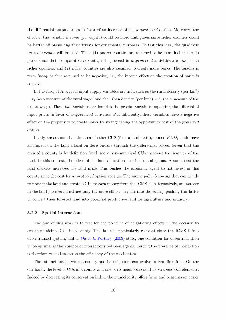
the differential output prices in favor of an increase of the unprotected option. Moreover, the

effect of the variable income (per capita) could be more ambiguous since richer counties could

be better off preserving their forests for ornamental purposes. To test this idea, the quadratic

term of income will be used. Thus, (1) poorer counties are assumed to be more inclined to do

parks since their comparative advantages to proceed in unprotected activities are lower than

richer counties, and (2) richer counties are also assumed to create more parks. The quadratic

term incsqj is thus assumed to be negative, i.e., the income effect on the creation of parks is

concave.

In the case, of Ri,j , local input supply variables are used such as the rural density (per km2)

rurj (as a measure of the rural wage) and the urban density (per km2) urbj (as a measure of the

urban wage). These two variables are found to be proxies variables impacting the differential

input prices in favor of unprotected activities. Put differently, these variables have a negative

effect on the propensity to create parks by strengthening the opportunity cost of the protected

option.

Lastly, we assume that the area of other CUS (federal and state), named FEDj could have

an impact on the land allocation decision-rule through the differential prices. Given that the

area of a county is by definition fixed, more non-municipal CUs increases the scarcity of the

land. In this context, the effect of the land allocation decision is ambiguous. Assume that the

land scarcity increases the land price. This pushes the economic agent to not invest in this

county since the cost for unprotected option goes up. The municipality knowing that can decide

to protect the land and create a CUs to earn money from the ICMS-E. Alternatively, an increase

in the land price could attract only the more efficient agents into the county pushing this latter

to convert their forested land into potential productive land for agriculture and industry.

3.2.2 Spatial interactions

The aim of this work is to test for the presence of neighboring effects in the decision to

create municipal CUs in a county. This issue is particularly relevant since the ICMS-E is a

decentralized system, and as Oates & Portney (2003) state, one condition for decentralization

to be optimal is the absence of interactions between agents. Testing the presence of interaction

is therefore crucial to assess the efficiency of the mechanism.

The interactions between a county and its neighbors can evolve in two directions. On the

one hand, the level of CUs in a county and one of its neighbors could be strategic complements.

Indeed by decreasing its conservation index, the municipality offers firms and peasants an easier

10

climate to make profits and to extend their activities. Moreover, a new firm could vote with its

feet (Tiebout 1956) and choose the municipality where the environmental standards are lower

to settle down. This way, a race to the bottom could be observed 12.

On the other hand, if we think in terms of the profitability of the two options, conservation

and exploitation, we could expect conservation decisions to be strategic substitutes. The creation

of new CUs by a county could have two effects. Firstly, since municipalities compete for a

fixed pool of money, when a given municipality creates new CUs, it decreases the amount

transferred by the state for each CUs, thus decreasing the profitability of the conservation

option. Secondly, the creation of new CUs decreases the stock of lands available for economic

production in a particular area. Then, it increases the value of plots available for economic

production and then the profitability of the exploitation option. A municipality could therefore

decide to increase its supply of land for economic agents (by decreasing its number of CUs),

in order to attract peasants and firms when its neighbor is decreasing its supply. We could

therefore expect protection decisions to be strategic substitutes.

From our theoretical framework, the land-allocation decision-rule for the plot i in the county

j becomes :

Dunprotectedij (Qprotectedk , FEDj , popj , indj , agrj , incj , incsqj , urbj , rurj). (9)

where Qprotectedk is the level of CUs in the neighboring county k which is assumed to influence

the profitability of the protected and unprotected options.

A land use decision-rule such as equation 9 leads to the equation which will be estimated

and presented in the following section 4.1.

4 Empirical strategy

4.1 Econometric model and data used

To estimate the presence of interactions between municipalities in their conservation deci-

sions, we borrow the methodology used in the tax-competition and public spending literature

(see for example Case et al. (1993), Brueckner (2003), Lockwood & Migali (2009) or Rota-

Graziosi et al. (2010)). We estimate a Spatial AutoRegressive (SAR) model, where the spatially

lagged endogenous variable is a weighted sum of neighbors’ decisions, such as :

12. In practice, there is no means to distinguish between a race to the top and a race to the bottom, but only

to find strategic complementarity between decisions. However, our theoretical analysis leads us to think that if

decisions are effectively strategic complements, they will lead to a race to the bottom.

11

P ∗ = ρWP ∗ + βX + ε (10)

where P ∗ is a N × 1 vector of the propensity to create a municipal CUs by a county. N

is the number of municipalities in the sample, here 399. X is a M × N matrix of our M

explanatory variables influencing the differential potential profit between land use conversion

and land conservation previously defined (pop, ind, agr, inc, incsq, rur, urb and FED) and β

is a vector of their corresponding coefficients. ε is a N×1 vector of residuals. WP ∗ is a spatially

lagged endogenous variable, where W is a N ×N contiguity matrix of which each element wjk

takes the value of 1 if two counties share a common border, 0 otherwise (where j identifies

a municipality different from municipality k). Hence, ρ capture the presence of interactions

between municipalities.

The dependent variable is latent, i.e., cannot be observed for p∗ < 0. Indeed, there is a large

number of zero observations in our sample. In 2010, 342 municipalities over 399 do not create

municipal CUs. It is hard to think that each municipality is in exactly the same situation. We

can therefore argue that censoring is at stake and that there exist negative profits unmeasured

by our dependent variable. Therefore, we have :

pj,t = 0 if p∗j,t ≤ 0

pj,t = p∗j,t otherwise,

where pj,t is the observed dependent variable. Following Chomitz & Gray (1996), we account

for this censoring using a tobit model, where the conditional distribution of pj,t given all other

parameters is a truncated normal distribution, constructed by truncating distribution from the

left at 0.

Finally, the following expanded form of the spatial autoregressive tobit models is :

p∗j,t2010 = ρ

J∑j 6=k

wjkp∗k,t + βpj,t2000 + δFEDj,t2010 + α1popj + α2indj + α3agrj + α4incj

+ α5incsqj + α6urbj + α7rurj + α8Curitiba+ µr + ϑi,t2010 , (11)

where the observed dependent variable, pj,t2010 , is the MCF of municipal parks of county j

in 2010 defined in section 2.2.

pj,t2000 represent the initialMCF in 2000. FEDj,t2010 isMCF of other CUs (federal and state

CUs) in the county i in 2010. popj , urbj and rurj are respectively the average annual population

12

growth, urban density and rural density between 2000-2010. indj (agrj) is the average ratio

between the GDP of industrial (agricultural) activities and the total municipal GDP between

2000 and 2008. incj is the annual average GDP per capita between 2000 and 2008 and incsqj ,

its squared equivalent. Curitiba is a dummy variable which takes a value of 1 for the capital

of Parana namely Curitiba and 0 otherwise to control for the strong differences of this county

compared to the others. µr is a micro-region dummy representing a legally defined administrative

area consisting of groups of municipalities bordering urban areas. This dummy allows to ckeck

for unobserved fixed effects shared by same neighboring counties. In the state of Parana, 39

micro-regions are censused for 399 counties.

Data concerning CUs (pj,t2010 , pj,t2000 and FEDj,t2010) are taken from the ICMS-E official

website 13. All other variables come from the IPEA DATABASE 14 (see table 5 page 28 in

appendix for more information on descriptive statistics).

4.2 Estimator

The estimation of parameters from spatial autoregressive tobit model represent a com-

putational challenge and cannot be done via analytic methods, such as maximum likelihood.

Therefore we rely on the bayesian approach developed by LeSage (1999), LeSage (2000), LeSage

& Pace (2009) and applied by Autant-Bernard & LeSage (2011).

In this approach, the unobserved negative profits associated with the censored 0 observations

are considered as parameters to estimate. The model is estimated via MCMC (Monte Carlo

Markov Chain) estimation procedure. The procedure uses the Geweke m-steps Gibbs sampler

to produce draws from a multivariate truncated normal distribution in order to generate the

unobserved negative utilities associated with the censored 0 observations 15 16.

4.3 Interpretation of the coefficients estimated

Coefficients from a SAR model cannot be interpreted directly. Indeed there is an implicit

form behind the model presented in equation 10. It can be rewritten as :

13. Data downloadable on this website http ://www.icmsecologico.org.br/.

14. Data downloadable on this website http ://www.ipeadata.gov.br/.

15. The m-steps correspond to the number of draws. Following LeSage & Pace (2009), considering our sample

size(N=399), we choose m=10 even if could be relatively computationally challenging.

16. In addition, to produce estimates that will be robust in the presence of non-constant variance of disturbances

(heteroscedasticity) and outliers, it is assumed that, in the development of the Gibbs sampler, the hyperparameter

r that determines the extent to which the disturbances take on a leptokurtic character is stated at 4 as suggested

by LeSage (1999).

13

P ∗ − ρWP ∗ = βX + ε (12)

P ∗(IN − ρW ) = βX + ε (13)

P ∗ = (IN − ρW )−1βX + (IN − ρW )−1ε (14)

As we can see from equation 14, ∂p∗

∂x′ 6= β, but ∂p∗

∂x′ = (IN − ρW )−1β. This occurs because of

the spillovers generated by the decisions of neighboring counties. To interpret the coefficients of a

spatial model, the researcher has to calculate the direct impact of a variable, its indirect impact

and the total impact (equal to the direct impact plus the indirect one). Indeed, a change on an

explanatory variable in a particular region will affect the p∗ value of this region (direct impact),

but also the other regions because of the spatial spillovers (the indirect impact). Computation

details of these impacts are clearly described in (LeSage & Pace 2009, p.33-39).

5 Results

5.1 Neighboring effects and created CUs

We estimated the influence of neighbors decision as well as several economic indicators on

the propensity of creating parks by a municipality. The Biodiversity Conservation coefficient

used by the state of Parana to redistribute the ICMS-E is used as dependent variable. In all

regressions, the contiguity spatial weight matrix is used to represent the prior strength between

two counties. Our results come from the estimation of a baysesian spatial tobit model using

1 step in the gibbs sampler and 1000 draws in the MCMC procedure 17. Our main results are

presented in table 1, where the first column present the value of the coefficients (β), the second

colmun the value of the direct impact of the explanatory variable, the third column the indirect

impact and the fourth the total impact.

17. With 10% of the draws used as burn-in.

14

Table 1 – Spatial interactions and MCF

Dependent variable : MCF 2010

n=1000, m=1

Variable Coefficient Direct Indirect Total

ρ -0.007961**

(0.015)

MCF2000 2.147355*** 2.159819*** -0.017943** 2.141876***

(0.000) (0.000) (0.036) (0.000)

FED2010 0.046348 0.04671 -0.000395 0.046315

(0.408) (0.417) (0.502) (0.417)

pop -0.000087 -0.000099 0.000001 -0.000098

(0.732) (0.718) (0.724) (0.718)

agr -0.120156*** -0.121699*** 0.001038* -0.120661***

(0.000) (0.000) (0.071) (0.000)

ind -0.045715 -0.046228 0.0004 -0.045827

(0.130) (0.129) (0.273) (0.129)

inc 0.007792 0.007482 -0.000067 0.007415

(0.763) (0.773) (0.790) (0.773)

incsq -0.002343 -0.00224 0.00002 -0.00222

(0.699) (0.714) (0.744) (0.714)

rur -0.000506 -0.000507 0.000004 -0.000503

(0.193) (0.212) (0.317) (0.212)

urb -0.000005 -0.000005 -0.000000 -0.000005

(0.738) (0.725) (0.739) (0.725)

Curitiba -0.22267*** -0.223891*** 0.001851* -0.22204***

(0.004) (0.004) (0.080) (0.004)

intercept -0.033999

(0.277)

Notes : ***=significant at the 1 percent level, **=significant at the 5 percent

level, *=significant at the 10 percent level. p-values associated to the reported

coefficients are in parentheses. n correspond to the number of draws and m

to the number of steps in the gibbs sampler. We allow for heteroscedasticity

in the error terms by setting the value of the hyperparameter r to 4.

Negative spatial interactions between counties are found (ρ < 0) suggesting that a county

is more inclined to create municipal CUs if their neighboring counties decrease the number of

their CUs. This way, this result points out that the hypothesis of profitability, predicted by the

theoretical model, seems to be at stake in the choice of creating municipal CUs in the state

of Parana between 2000 and 2010. This way, it is more profitable for a county to convert its

natural land for agricultural or industrial activities if their neighboring counties have preferred

to create CUs and be awarded by the ICMS-E. The design of the ICMS-E is an explanation of

15

these behaviors since the pool of money is fixed, thus leading a county to not be incited to enter

into the mechanism and so to be more inclined to convert its natural land for economic purposes.

This result is linked to the descriptive statistics proposed in section 2.3 and could explain the

stable trend in the creation of municipal CUs in the last decade after a strong upward trend

in the first years of the implementation of the ICMS-E. Concerning the other economic factors

assumed to have an effect on the land allocation rule-decision of a county (through their effects

on the differential profit between land uses option), the population variables have the expected

negative coefficient but are not significant. Moreover, the structure of the county’s economy is

found to be important to explain the propensity to create municipal CUs. In fact, the more the

share of agriculture is important in the municipal activities, the less the propensity to create

municipal CUs. This result points out the role of economic activities in the propensity to create

CUs. More developed counties in terms of agricultural activities can be more encouraged to

develop their activities to earn money from the ICMS which awards counties on the basis of

their created value added. Besides, the Table 2 provides the estimated direct, indirect and total

effects of each explanatory variable. Recall that direct impact can be interpreted as a marginal

impact, the indirect one as a spatial spillover effect and total one as a summary measure of

the total impact associated with changes in each explanatory variable. All significant effects

previously presented (for population growth and the weight of agriculture and industry) are

found to be mainly direct effects. However, we observe indirect effect effect of lower magnitude

and of the opposite sign, which is due to the substitutable nature of conservation decisions.

5.2 Robustness checks

5.2.1 Taking only account of the size of protected areas

As our first robustness check, we use a different measure of the environmental performance

of a county. Indeed, the Municipal Conservation Factor used to redistribute the ICMS-E is equal

to the ratio of protected areas on total area of a county, weighed by a measure of the intensivity

of the protection, the ”quality factor”. We choose to use only the ratio of protected areas on

total land - the quantity tatio - as dependent variable. This will allow us to check the robustness

of our first result (the substitutability in conservation decisions) and to see is the driving forces

tested influence the way a country choose to improve its protection of land (i.e., in an intensive

or extensive manner). Table 2 presents results for the quantity ratio as dependent variable.

16

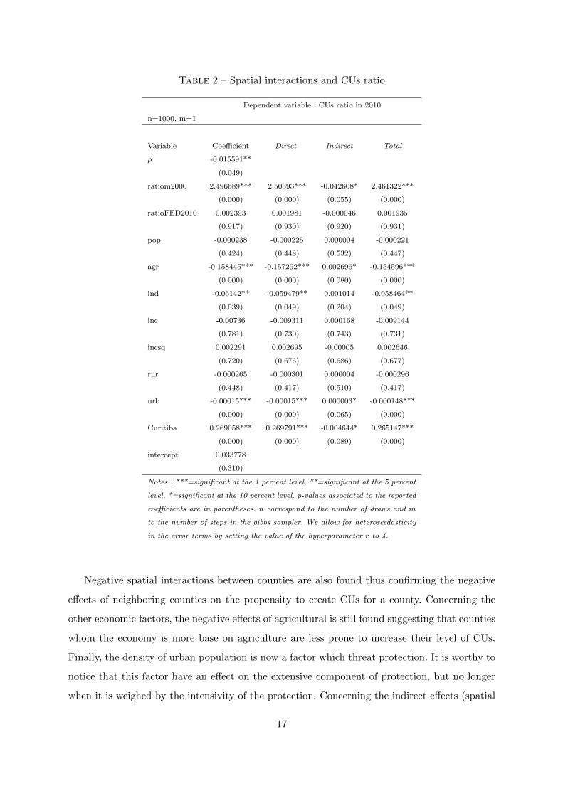
Table 2 – Spatial interactions and CUs ratio

Dependent variable : CUs ratio in 2010

n=1000, m=1

Variable Coefficient Direct Indirect Total

ρ -0.015591**

(0.049)

ratiom2000 2.496689*** 2.50393*** -0.042608* 2.461322***

(0.000) (0.000) (0.055) (0.000)

ratioFED2010 0.002393 0.001981 -0.000046 0.001935

(0.917) (0.930) (0.920) (0.931)

pop -0.000238 -0.000225 0.000004 -0.000221

(0.424) (0.448) (0.532) (0.447)

agr -0.158445*** -0.157292*** 0.002696* -0.154596***

(0.000) (0.000) (0.080) (0.000)

ind -0.06142** -0.059479** 0.001014 -0.058464**

(0.039) (0.049) (0.204) (0.049)

inc -0.00736 -0.009311 0.000168 -0.009144

(0.781) (0.730) (0.743) (0.731)

incsq 0.002291 0.002695 -0.00005 0.002646

(0.720) (0.676) (0.686) (0.677)

rur -0.000265 -0.000301 0.000004 -0.000296

(0.448) (0.417) (0.510) (0.417)

urb -0.00015*** -0.00015*** 0.000003* -0.000148***

(0.000) (0.000) (0.065) (0.000)

Curitiba 0.269058*** 0.269791*** -0.004644* 0.265147***

(0.000) (0.000) (0.089) (0.000)

intercept 0.033778

(0.310)

Notes : ***=significant at the 1 percent level, **=significant at the 5 percent

level, *=significant at the 10 percent level. p-values associated to the reported

coefficients are in parentheses. n correspond to the number of draws and m

to the number of steps in the gibbs sampler. We allow for heteroscedasticity

in the error terms by setting the value of the hyperparameter r to 4.

Negative spatial interactions between counties are also found thus confirming the negative

effects of neighboring counties on the propensity to create CUs for a county. Concerning the

other economic factors, the negative effects of agricultural is still found suggesting that counties

whom the economy is more base on agriculture are less prone to increase their level of CUs.

Finally, the density of urban population is now a factor which threat protection. It is worthy to

notice that this factor have an effect on the extensive component of protection, but no longer

when it is weighed by the intensivity of the protection. Concerning the indirect effects (spatial

17

externalities), two variables have a significant effect. First is the negative initial level of quality

(in 2000) suggesting that the more was the initial level of neighbors, the less the propensity

for the county to increase the quality of its CUs. The second significant indirect impact is the

positive effect of agriculture. Thus, the greater the weight of agriculture in the neighbors of a

municipality, the greater the propensity to create CUs in this county.

5.2.2 Checking the consistency of the estimator

Since the bayesian spatial tobit is a new estimator and that few researcher have used it, we

provide several robustness tests on the estimator itself. Indeed, to our knowledge, it have been

proposed in the article of LeSage (2000) and the manuals of LeSage (1999) and LeSage & Pace

(2009), but to the best of our knowledge, have only been applied in Autant-Bernard & LeSage

(2011).

The following regressions are run with different number of m-steps (m = 1, m = 10 or

m = 20) of the Gibbs sampler process and different number of draws (n=1,000 ; 10,000). Ro-

bustness tests are made on the estimation procedure since the main computational challenge

using a Bayesian framework is the state of some parameters such as the number of draws or the

number of m-step used in the computation of the estimated negative utilities for the censored

observations of the dependent variable (LeSage & Pace 2009).

The first robustness check on the number of steps in the Gibbs sampler process, aims at

testing the accuracy of the computed vector of parameters which replaces the unobserved latent

utility (here for p∗j,t < 0) (LeSage & Pace 2009, p.287).

The second test consists in increasing the number of draws and comparing the inferences

based on a smaller set of draws (here n=1,000) to those resulting from a larger set of draws

(here n=10,000) in order to evaluate the stability in the parameter values found. The basic

assumption is that if the inferences are identical, then the estimator can be assumed to be

consistent.

Tables 3 provide results with the MCF coefficients as dependent variable for respectively

1, 10 and 20 steps of the Gibbs sampler process, with 1,000 and 10,000 draws . The spatial

interactions are still found to be negative and significant as are the urban density, the agricultural

ratio and the industrial one. The level of created CUs in 2000 is found to have a significant and

negative indirect effect suggesting the presence of negative neighboring effects on the propensity

to create CUs. Also, urban density is now found to have a significant positive indirect effect.

This reinforces the role of urban density in the decision to create CUs. If the neighbor of a

18

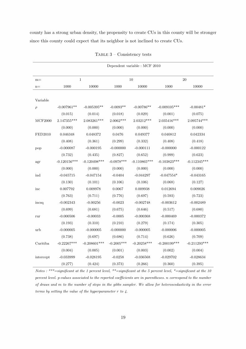
county has a strong urban density, the propensity to create CUs in this county will be stronger

since this county could expect that its neighbor is not inclined to create CUs.

Table 3 – Consistency tests

Dependent variable : MCF 2010

m= 1 10 20

n= 1000 10000 1000 10000 1000 10000

Variable

ρ -0.007961** -0.005395** -0.0093** -0.00786** -0.009105*** -0.00481*

(0.015) (0.014) (0.018) (0.029) (0.001) (0.075)

MCF2000 2.147355*** 2.083261*** 2.0062*** 2.03212*** 2.035416*** 2.095744***

(0.000) (0.000) (0.000) (0.000) (0.000) (0.000)

FED2010 0.046348 0.048372 0.0476 0.049377 0.040812 0.042334

(0.408) (0.361) (0.299) (0.332) (0.408) (0.418)

pop -0.000087 -0.000195 -0.000000 -0.000111 -0.000000 -0.000122

(0.732) (0.435) (0.827) (0.652) (0.999) (0.623)

agr -0.120156*** -0.120498*** -0.0978*** -0.110865*** -0.103823*** -0.112345***

(0.000) (0.000) (0.000) (0.000) (0.000) (0.000)

ind -0.045715 -0.047154 -0.0404 -0.044297 -0.047554* -0.043165

(0.130) (0.101) (0.106) (0.106) (0.068) (0.127)

inc 0.007792 0.009978 0.0067 0.009938 0.012694 0.009026

(0.763) (0.711) (0.776) (0.697) (0.593) (0.723)

incsq -0.002343 -0.00256 -0.0023 -0.002748 -0.003612 -0.002489

(0.699) (0.681) (0.675) (0.646) (0.517) (0.680)

rur -0.000506 -0.00033 -0.0005 -0.000368 -0.000469 -0.000372

(0.193) (0.310) (0.210) (0.279) (0.174) (0.305)

urb -0.000005 -0.000005 -0.000000 -0.000005 -0.000006 -0.000005

(0.738) (0.697) (0.686) (0.714) (0.626) (0.709)

Curitiba -0.22267*** -0.208601*** -0.2005*** -0.20258*** -0.200199*** -0.211293***

(0.004) (0.005) (0.001) (0.003) (0.002) (0.004)

intercept -0.033999 -0.028195 -0.0258 -0.036568 -0.029702 -0.028634

(0.277) (0.424) (0.373) (0.266) (0.360) (0.395)

Notes : ***=significant at the 1 percent level, **=significant at the 5 percent level, *=significant at the 10

percent level. p-values associated to the reported coefficients are in parentheses. n correspond to the number

of draws and m to the number of steps in the gibbs sampler. We allow for heteroscedasticity in the error

terms by setting the value of the hyperparameter r to 4.

19

6 Conclusion

The aim of this paper was to assess the efficiency of the ICMS-E by testing the presence of

strategic interactions between Brazilian counties in the state of Parana. It is a fiscal transfer

from the state to municipalities on the basis of the performance of each county in the creation

and management of CUs. This way, the ICMS-E can be viewed as a Payment for Environmental

Services (PES).

This fiscal scheme is important since it is a form of PES which can be implemented without

external source of financing and at very low transaction costs. However, since the system is

decentralized, its efficiency could be threatened by the presence of interactions between muni-

cipalities when they decide to set their lands aside for protection.

Therefore, this study tries to investigate if the behavior of neighboring counties in terms of

created municipal CUs has an effect on the propensity for a county to create municipal CUs

between 2000 and 2010 in the state of Parana. The choice of the time-span analysis is motivated

by the availability of data but is interesting due to the fact that, in this period, the level of

created CUs seems to have reached a stationary level after a strong upward trend in the first

decade of the implementation of the ICMS-E (1992-2000).

From a land use model and a spatial autoregressive Bayesian tobit model, the results suggest

the presence of negative spatial interactions between counties. These negative spatial externali-

ties can be explained by the hypothesis of profitability which states that the county will choose

the use which maximizes its profit. In our case a municipality will prefer to develop economic

activities, to attract peasants and firms from a neighbor who have decided to create CUs. The

fact that in the ICMS-E a fixed pool of money is shared between counties explain and strengthen

this effect.

The results do not highlight a race to the bottom between counties which would have finally

questioned the efficiency of the ICMS-E. However, we observe strategic substitutability between

conservation decisions which seems to lead the mechanism to reach an equilibrium. In a way, the

mechanism seems to be efficient, because this result suggests that the behavior of municipalities

is driven by an optimization process and that they integrate the decision of their neighbors in

their calculus.

However, remark that there is no reason for the shared pool of money to lead to the optimal

level of land set aside for protection. Moreover, it seems that municipalities do not intend to

provide a public good but are more subject to a profitability calculus. This way, the design of

20

the ICMS-E, via the definition of the quality weighting factor, seems crucial.

To conclude, the ICMS-E has had great success and has allowed to increase the number

of CUs in Parana. This experience should be viewed as a new and interesting tool to finance

local public good without external funding, but being aware of the potential negative spatial

interactions which can occur.

References

Andersen, L. E., Granger, C. W. J., Reis, E. J., Weinhold, D. & Wunder, S. (2002), The dynamics

of deforestation and economic growth in the brazilian amazon, Cambridge University Press.

Arcand, J.-L., Guillaumont, P. & Jeanneney-Guillaumont, S. (2008), ‘Deforestation and the real

exchange rate’, Journal of Development Economics 86(2), 242–262.

Autant-Bernard, C. & LeSage, J. P. (2011), ‘Quantifying knowledge spillovers using spatial

econometric models’, Journal of Regional Science 51(3), 471–496.

Brooks, T. & Balmford, A. (1996), ‘Atlantic forest extinctions’, Nature 380(6570), 115.

Brooks, T., Tobias, J. & Balmford, A. (1999), ‘Deforestation and bird extinctions in the atlantic

forest’, Animal Conservation 2(3), 211–222.

Brueckner, J. (2003), ‘Strategic interaction among governments : an overview of empirical stu-

dies’, International regional science review 26, 175–188.

Case, A. C., Rosen, H. S. & Hines, J. J. (1993), ‘Budget spillovers and fiscal policy interdepen-

dence : Evidence from the States’, Journal of Public Economics 52(3), 285–307.

Chomitz, K. M. & Gray, D. A. (1996), ‘Roads, land use, and deforestation : A spatial model

applied to belize’, The World Bank Economic Review 10, 487–512.

Chomitz, K. M. & Thomas, T. S. (2001), ‘Geographic patterns of land use and land intensity

in the brazilian amazon’, World Bank Policy Research Working Paper No. 2687.

Farley, J., Aquino, A., Daniels, A., Moulaert, A., Lee, D. & Krause, A. (2010), ‘Global mecha-

nisms for sustaining and enhancing pes schemes’, Ecological Economics 69(11), 2075–2084.

Feres, J. G. & da Motta, R. S. (2004), Country case : Brazil, in R. S. da Motta, ed., ‘Economic

instruments for water management : the cases of France, Mexico, and Brazil’, Edward Elgar

Publishing, pp. 97–133.

21

Grieg-Gran, M. (2000), ‘Fiscal incentives for biodiversity conservation : The icms ecologico in

brazil’, Discussion Papers IIED (00-01).

Kaimowitz, D. & Angelsen, A. (1998), Economic models of tropical deforestation : a review,

Cifor.

LeSage, J. (1999), The theory and practice of spatial econometrics., 1 edn, Online Manuel.

LeSage, J. P. (2000), ‘Bayesian estimation of limited dependent variable spatial autoregressive

models’, Geographical Analysis 32(1), 19–35.

LeSage, J. & Pace, R. K. (2009), Introduction to Spatial Econometrics (Statistics : A Series of

Textbooks and Monographs), 1 edn, Chapman and Hall/CRC.

Lockwood, B. & Migali, G. (2009), ‘Did the single market cause competition in excise taxes ?

evidence from EU countries’, Economic Journal 119(536), 406–429.

Loureiro, W., Pinto, M. A. & Joslin Motta, M. n. (2008), ‘Legislao atualizada do icms ecolgico

por biodiversidade’, Governo do Parana .

May, P. H., Neto, F. V., Denardin, V. & Loureiro, W. (2002), Selling Forest Environmental

Services : Market-based Mechanisms for Conservation and Development, Earthscan Publica-

tions, chapter Using fiscal instruments to encourage conservation : Municipal responses to

the ecologicalvalue-added tax in Parana and Minas Gerais, Brazil, pp. 173–199.

Myers, N., Mittermeier, R. A., Mittermeier, C. G., Da Fonseca, G. A. & Kent, J. (2000),

‘Biodiversity hotspots for conservation priorities.’, Nature 403(6772), 853–858.

Nelson, G. & Geoghegan, J. (2002), ‘Deforestation and land use change : sparse data environ-

ments’, Agricultural Economics 27, 201–216.

Oates, W. & Portney, P. (2003), Handbook of environmental economics, Vol. 1, chapter The

political economy of environmental policy, pp. 325–354.

Pfaff, A. S. (1999), ‘What drives deforestation in the brazilian amazon ? evidence from satellite

and socioeconomic data’, Journal of Environmental Economics and Management 37(1), 26–

43.

Putz, S., Groeneveld, J., Alves, L., Metzger, J. & Huth, A. (2011), ‘Fragmentation drives tropical

forest fragments to early successional states : A modelling study for brazilian atlantic forests’,

Ecological Modelling 222(12), 1986 – 1997.

22

Ring, I. (2008), ‘Integrating local ecological services into intergovernmental fiscal transfers : the

case of the ecological icms in brazil’, Land Use Policy 25(4), 485–497.

Rota-Graziosi, G., Caldeira, E. & Foucault, M. (2010), ‘Decentralization in africa and the nature

of local governments’ competition : evidence from benin’, CERDI-Working Paper (2010.19).

Tiebout, C. M. (1956), ‘A pure theory of local expenditures’, Journal of Political Economy

64, 416.

Verssimo, A., Le Boulluec Alves, Y., Pantoja da Costa, M., Riccio de Carvalho, C., Born, G. C.,

Talocchi, S. & Born, R. H. (2002), Payment for environmental services : Brazil, Technical

report, Fundacin PRISMA.

Vogel, J. H. (1997), ‘The successful use of economic instruments to foster sustainable use of

biodiversity : six case studies from latin america and the caribbean’, Biopolicy 2.

23

7 Appendix

7.1 Parana in Brazil

Figure 1 – Parana in Brazil

Source : Encyclopaedia Britannica

24

7.2 Calculation of the ICMS-E : the conservation factor

Table 4 – Conservation factor FCn for different management categories n of protected areas

in Parana

Management category Federal State Municipal

Ecological research station 0.8 0.8 1

Biological reserve 0.8 0.8 1

Parks 0.7 0.7 0.9

Private natural heritage reserve (RPPN) 0.68 0.68 .

Area of relevant ecological interest 0.66 0.66 0.66

Forest 0.64 0.64 0.64

Indigenous area 0.45 . .

Buffer zones (Faxinais) . 0.45 .

Environmental protection area 0.08 0.08 0.08

Special, local areas of tourist interest 0.08 0.08 0.08

Source : Adapted from (Loureiro et al. 2008, p.73). A point (.) men-

tions that there is none CU of this nature. For instance, there is none

municipal or state indigenous area.

25

7.3 Creation of CUs over time

Figure 2 – Evolution of the creation of all CUs in Parana between 1991 and 2010

Note : Evolution of the areas (in hectare) of all conservation units (federal, state and

municipal) between 2000 and 2010.

Source : Authors’ calculation from May et al. (2002) and Grieg-Gran (2000), and authors’

collected data.

26

7.4 Descriptive statistics

Figure 3 – Evolution of the number of counties in the ICMS-E for municipal CUs'

&

$

%

Number of

counties : 399

ICMS-E in 2000 : 57

ICMS-E in 2010 : 53Not in ICMS-E in

2010 : 4

Not in ICMS-E in

2000 : 342

ICMS-E in 2010 : 13not ICMS-E in

2010 : 329

Note : Evolutions between 2000 and 2010 of the number of counties concerning by the

ICMS-E for the creation of municipal CUs.

Source : drafted by the authors

Figure 4 – Evolution of the number of counties in the ICMS-E'

&

$

%

Number of

counties : 399

ICMS-E in 2000 :

174

ICMS-E in 2010 :

170

Not in ICMS-E in

2010 : 4

Not in ICMS-E in

2000 : 225

ICMS-E in 2010 : 22not ICMS-E in

2010 : 203

Note : Evolutions between 2000 and 2010 of the number of counties concerning by the

ICMS-E, whatever the CUs.

Source : drafted by the authors

27

Table 5 – Summary statistics

Variable Mean (Std. Dev.) Min. Max. N

CUs ratio (2010) 0.0034 (0.0238) 0 0.2175 399

Coefficient quality (2010) 0.0018 (0.009) 0 0.1272 399

CUs ratio (2000) 0.0018 (0.0156) 0 0.1993 399

Coefficient quality (2000) 0.0013 (0.0093) 0 0.1695 399

CUs ratio (Federal, State) 2010 0.0444 (0.1322) 0 0.9876 399

Coefficient quality (Federal, State) 2010 0.0135 (0.0386) 0 0.3254 399

Population growth 2.2483 (11.7301) -38.4769 73.3038 399

Ratio agriculture 0.3051 (0.1484) 0.0004 0.6235 399

Ratio industry 0.1439 (0.1148) 0.0288 0.8336 399

Log GDP 1.6361 (0.3994) 0.8232 3.7569 399

Log GDP squared 2.836 (1.5153) 0.6777 14.1145 399

Rural population density 9.4345 (10.9149) 0 192.9066 399

Urban population density 51.1113 (233.5605) 0.8544 3918.803 399

Source : Authors’ calculation.

28