1

“Ecole IRISA” : distributedalgorithms and models

Course 1 : some fundamentals

• 1.1 Distributed programs• 1.2 Abstract behaviour• 1.3 Causality• 1.4 Lamport’s coding• 1.5 Vector clocks• 1.6 Interval approximation• 1.7 Notion of state for a distributed run• 1.8 Global checking of traces• 1.9 Distributed checking

C. Jard, October 2006

2

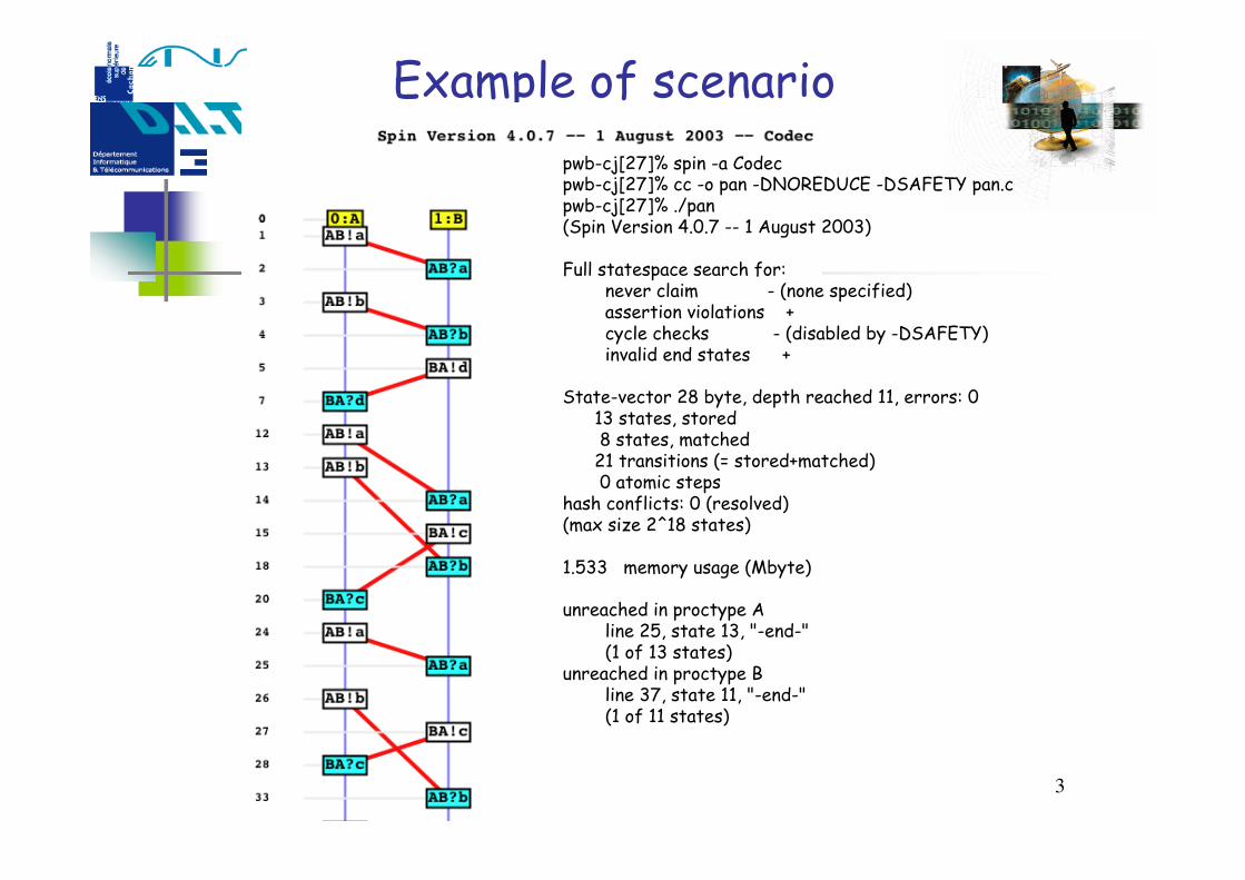
1. A simple protocol (in Promela/Spin) :a first distributed program

mtype = {a,b,c,d};

/* a : connect_request b : disconnect_request c : distant_disconnect_request d : disconnect_confirm*/

chan AB = [3] of {mtype};chan BA = [1] of {mtype};

active proctype B(){ do :: AB?b; :: AB?a; if :: AB?b; BA!d; :: BA!c fi od}

active proctype A(){

do :: AB!a; if :: BA?c; :: AB!b; if :: BA?c; :: BA?d fi fi od}

3

Example of scenariopwb-cj[27]% spin -a Codec pwb-cj[27]% cc -o pan -DNOREDUCE -DSAFETY pan.cpwb-cj[27]% ./pan(Spin Version 4.0.7 -- 1 August 2003)

Full statespace search for: never claim - (none specified) assertion violations + cycle checks - (disabled by -DSAFETY) invalid end states +

State-vector 28 byte, depth reached 11, errors: 0 13 states, stored 8 states, matched 21 transitions (= stored+matched) 0 atomic stepshash conflicts: 0 (resolved)(max size 2^18 states)

1.533 memory usage (Mbyte)

unreached in proctype A line 25, state 13, "-end-" (1 of 13 states)unreached in proctype B line 37, state 11, "-end-" (1 of 11 states)

4

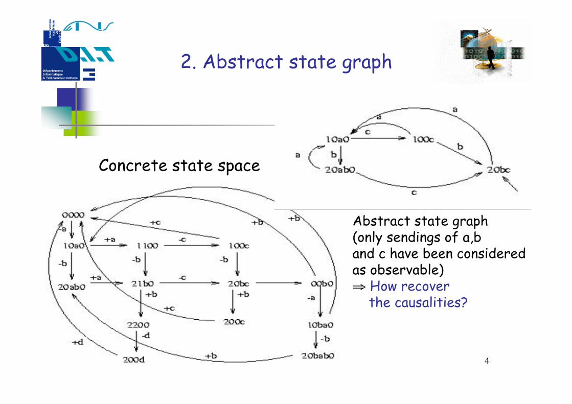
2. Abstract state graph

Concrete state space

Abstract state graph (only sendings of a,b and c have been consideredas observable)⇒ How recover the causalities?

5

3. Causality between observable events(Lamport 78)

• N sequential processes (P1 to Pn)• Processes perform events during their life. Some of them are

traced (the observable events)• Communication by passing messages synchronises the process

activity

c

e

fP1

P2

P3a

b d

g

h

6

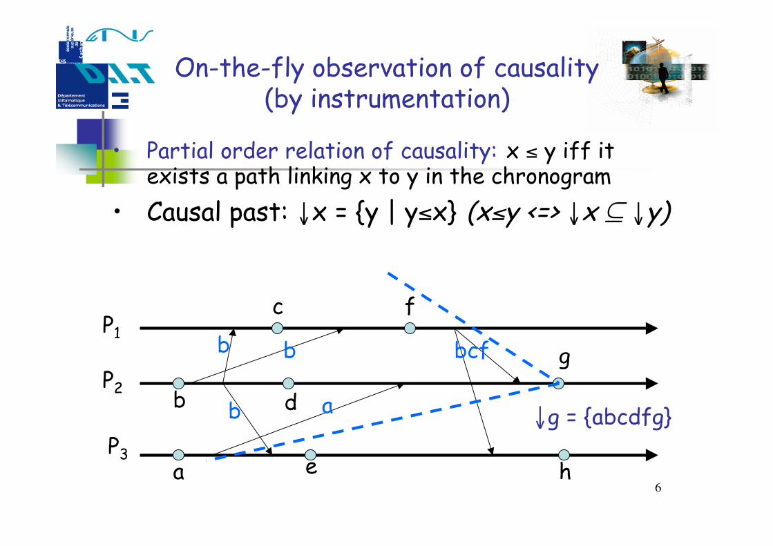
On-the-fly observation of causality(by instrumentation)

• Partial order relation of causality: x ≤ y iff itexists a path linking x to y in the chronogram

• Causal past: ↓x = {y | y≤x} (x≤y <=> ↓x ⊆ ↓y)

P1

P2

P3a

b d

g

h

↓g = {abcdfg}

b b

b a

c

e

f

bcf

7

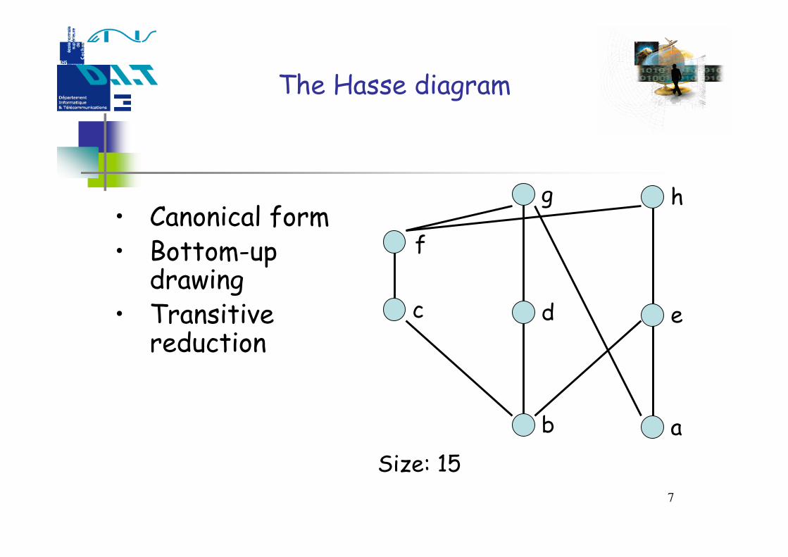
The Hasse diagram

• Canonical form• Bottom-up

drawing• Transitive

reduction

a

e

h

b

d

g

c

f

Size: 15

8

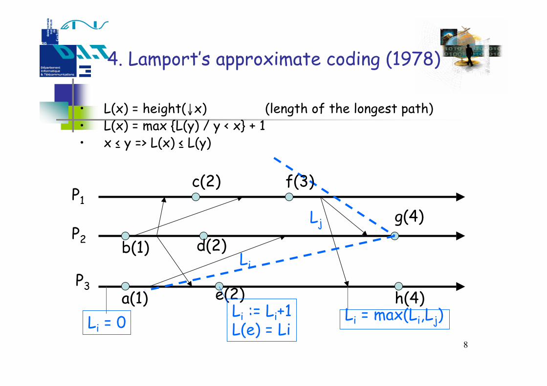
4. Lamport’s approximate coding (1978)

• L(x) = height(↓x) (length of the longest path)• L(x) = max {L(y) / y < x} + 1• x ≤ y => L(x) ≤ L(y)

P1

P2

P3a(1)

b(1) d(2)

g(4)

h(4)Li = max(Li,Lj)

Li

c(2)

e(2)

f(3)

Lj

Li = 0Li := Li+1L(e) = Li

9

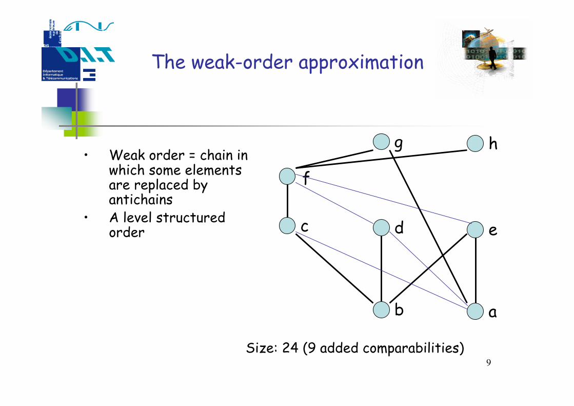
The weak-order approximation

• Weak order = chain inwhich some elementsare replaced byantichains

• A level structuredorder

a

e

h

b

d

g

c

f

Size: 24 (9 added comparabilities)

10

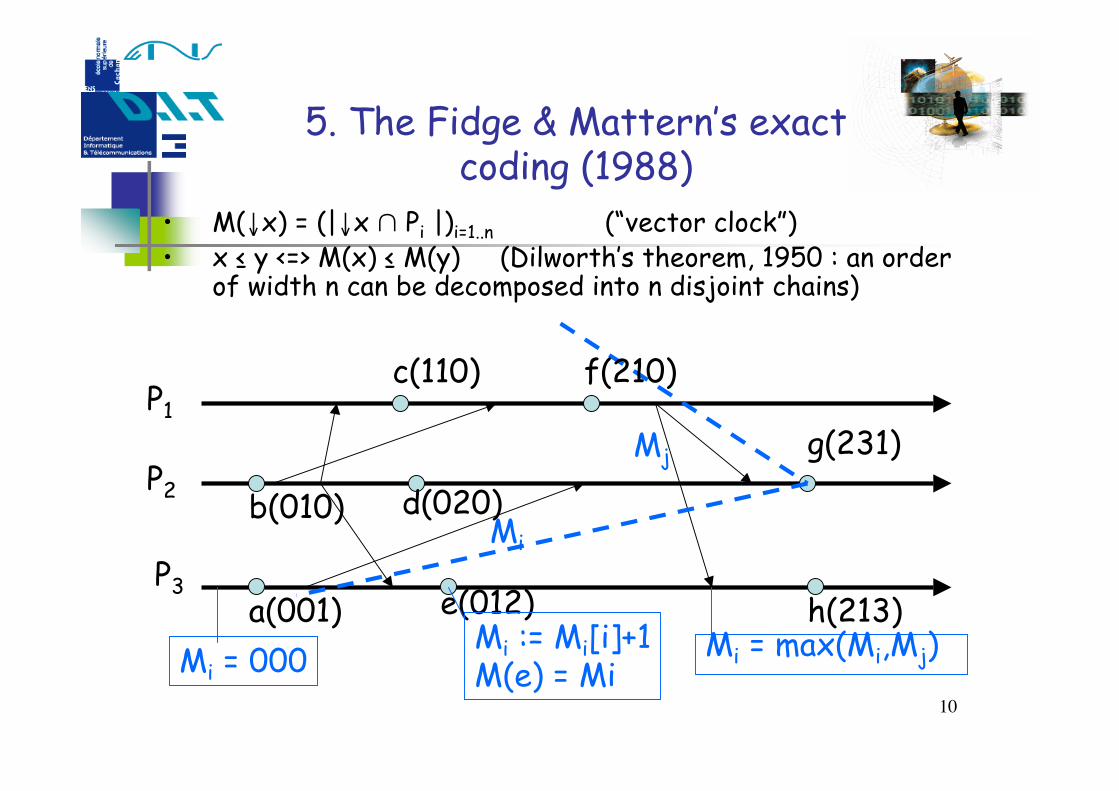
5. The Fidge & Mattern’s exactcoding (1988)

• M(↓x) = (|↓x ∩ Pi |)i=1..n (“vector clock”)• x ≤ y <=> M(x) ≤ M(y) (Dilworth’s theorem, 1950 : an order

of width n can be decomposed into n disjoint chains)

P1

P2

P3a(001)

b(010) d(020)

g(231)

h(213)Mi = max(Mi,Mj)

Mi

c(110)

e(012)

f(210)

Mj

Mi = 000Mi := Mi[i]+1M(e) = Mi

11

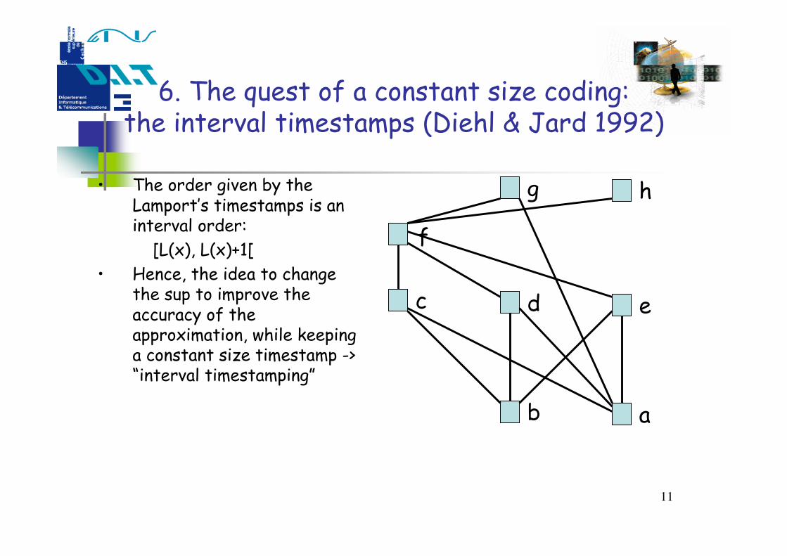
6. The quest of a constant size coding:the interval timestamps (Diehl & Jard 1992)

• The order given by theLamport’s timestamps is aninterval order: [L(x), L(x)+1[

• Hence, the idea to changethe sup to improve theaccuracy of theapproximation, while keepinga constant size timestamp ->“interval timestamping”

a

e

h

b

d

g

c

f

12

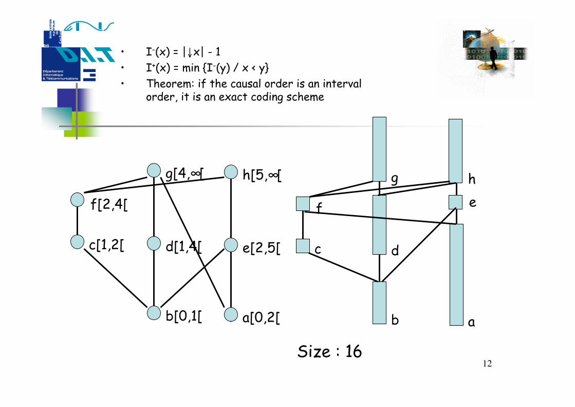
• I-(x) = |↓x| - 1• I+(x) = min {I-(y) / x < y}• Theorem: if the causal order is an interval

order, it is an exact coding scheme

a[0,2[

e[2,5[

h[5,∞[

b[0,1[

d[1,4[

g[4,∞[

c[1,2[

f[2,4[

a

e h

b

d

g

c

f

Size : 16

13

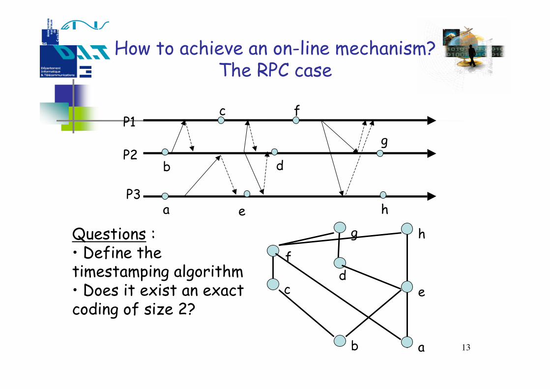
How to achieve an on-line mechanism?The RPC case

c

e

fP1

P2

P3a

b d

g

h

a

e

h

b

d

g

c

fQuestions :• Define thetimestamping algorithm• Does it exist an exactcoding of size 2?

14

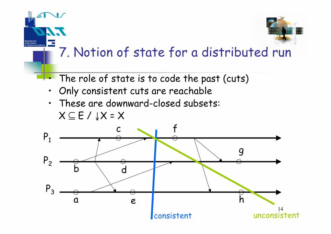
7. Notion of state for a distributed run

• The role of state is to code the past (cuts)• Only consistent cuts are reachable• These are downward-closed subsets:

X ⊆ E / ↓X = Xc

e

fP1

P2

P3a

b d

g

hconsistent unconsistent

15

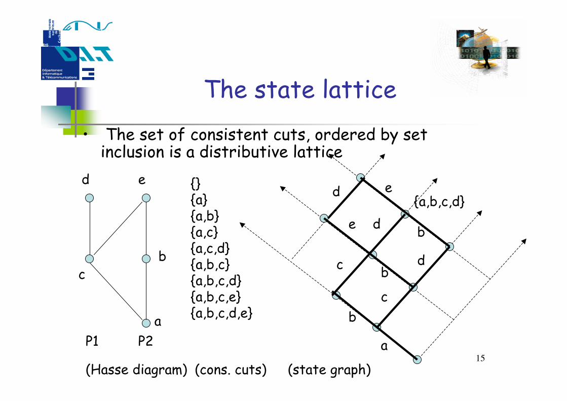
The state lattice• The set of consistent cuts, ordered by set

inclusion is a distributive lattice

(Hasse diagram)

P1 P2

d e

cb

a

{}{a}{a,b}{a,c}{a,c,d}{a,b,c}{a,b,c,d}{a,b,c,e}{a,b,c,d,e}

(cons. cuts)

a

c

c

b

b

b

d

d

d

e

e{a,b,c,d}

(state graph)

16

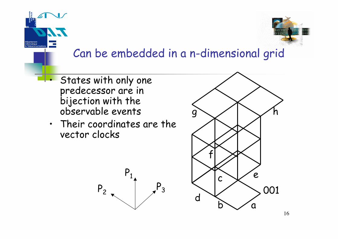
Can be embedded in a n-dimensional grid

• States with only onepredecessor are inbijection with theobservable events

• Their coordinates are thevector clocks

abd

e

h

c

g

f

001

P1

P3P2

17

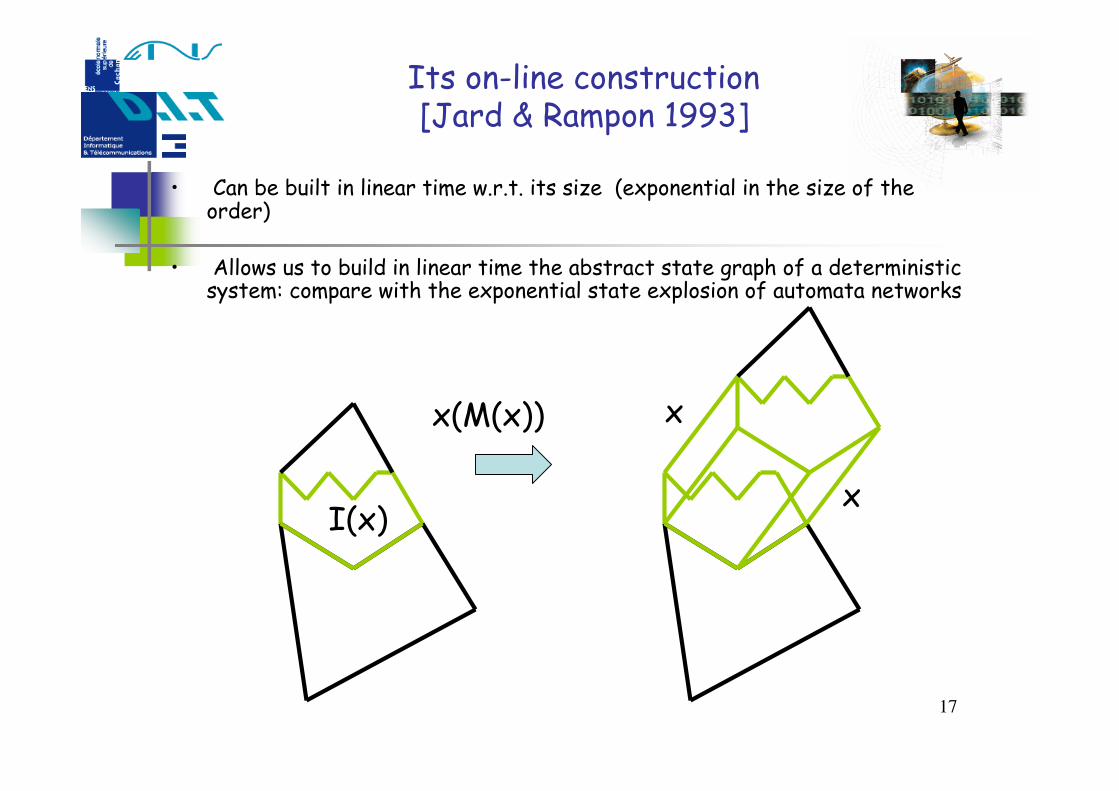
Its on-line construction[Jard & Rampon 1993]

• Can be built in linear time w.r.t. its size (exponential in the size of theorder)

• Allows us to build in linear time the abstract state graph of a deterministicsystem: compare with the exponential state explosion of automata networks

x(M(x))

I(x)x

x

18

An example of on-the-fly construction

P1 P2

d e

cb

a

a

c

c

b

b

b

d

d

d

e

e

aa

ba

b d

a

d

d

b

b

c

a

c

c

b

b

b

d

de

19

8. Trace checking(regular properties)

• Property Φ = <Σ,Q,q0,F,δ>,defines a langage L(Φ) = {u ∈ Σ* | δ*(u,q0) ∈ F}

• State graph: transitions labelled with Σ,

given a state I, Paths(I) is the set of words leading to I• I satisfies Φ iff Paths(I) intersects L(Φ)• Equivalently: I satisfies Φ iff Φ(I) intersects F where Φ(I) is the set of states of the automaton Φ reachable

by paths ending at I• A trace satisfies Φ iff the maximal state (Σ) satisfies Φ

20

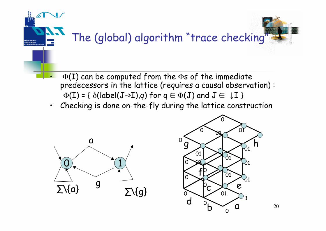
The (global) algorithm “trace checking”

• Φ(I) can be computed from the Φs of the immediatepredecessors in the lattice (requires a causal observation) :

Φ(I) = { δ(label(J->I),q) for q ∈ Φ(J) and J ∈ ↓I }• Checking is done on-the-fly during the lattice construction

0

abde

h

c

g

f1

a

g∑\{a} ∑\{g}

0

10

0 010

0 0101

010

0101

001

0

01

0 01 01

0

21

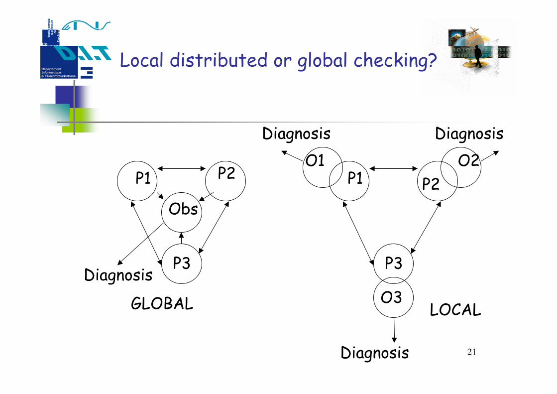
Local distributed or global checking?

P1 P2

P3

Obs

Diagnosis

P1 P2

P3

O1 O2

O3

Diagnosis Diagnosis

Diagnosis

GLOBAL LOCAL

22

Global :• Causal dependency

tracking• On-line construction of

the state lattice• Verification during

construction

Local :• Restricted class of

properties (causalflows)

• Distributed verification(timestamps extendedwith a stateinformation)

Distributed checking [Jard & Raynal 1995]

23

9. Distributed trace checking(local regular properties)

• Properties are on the causal past of the observableevents

• An observable event x satisfies a property Φ iff itexists a path ending in x in the Hasse diagram of theobserved order such that the corresponding path isaccepted by Φ

• Causal ordering case• Can be computed on-the-fly and in a distributed

manner

24

Principle

• The automaton Φ is know from all the processes• x satisfies Φ is locally computed on the process

which has produced x• The state information is acquired (and piggybacked)

by the messages of the observed execution• Each process Pi maintain 2 arrays: LOi[1..n] and

SLOi[1..n]. LOi[j] is the rank of the the last event observedPj in the current past of Pi. SLOi[j] is the corresponding stateinformation (of Φ) (when LOi[j] is maximal)

25

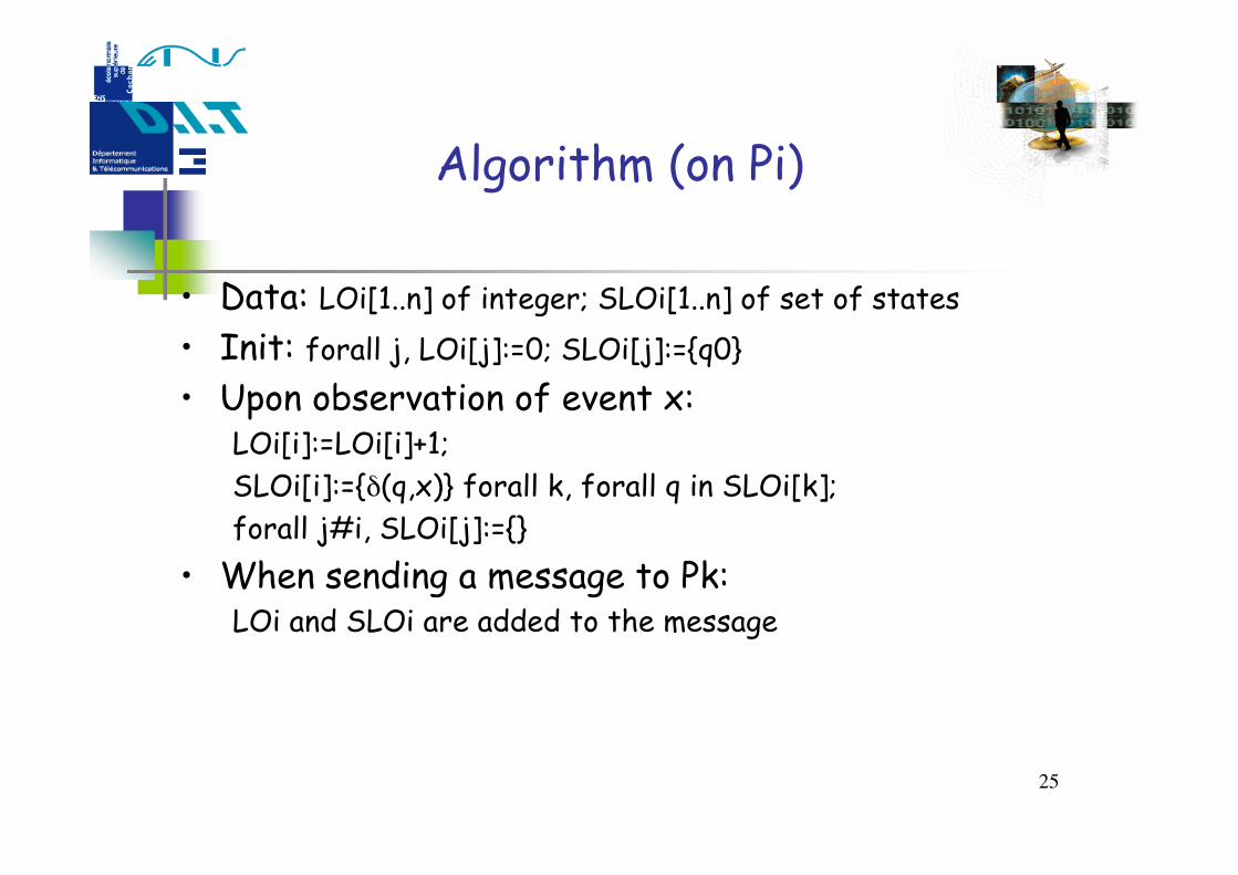
Algorithm (on Pi)

• Data: LOi[1..n] of integer; SLOi[1..n] of set of states• Init: forall j, LOi[j]:=0; SLOi[j]:={q0}• Upon observation of event x: LOi[i]:=LOi[i]+1; SLOi[i]:={δ(q,x)} forall k, forall q in SLOi[k]; forall j#i, SLOi[j]:={}• When sending a message to Pk: LOi and SLOi are added to the message

26

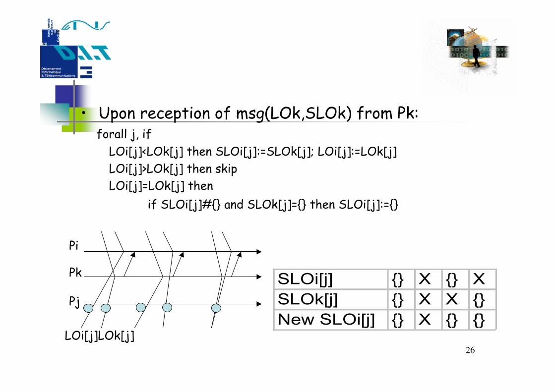
• Upon reception of msg(LOk,SLOk) from Pk: forall j, if LOi[j]<LOk[j] then SLOi[j]:=SLOk[j]; LOi[j]:=LOk[j] LOi[j]>LOk[j] then skip LOi[j]=LOk[j] then if SLOi[j]#{} and SLOk[j]={} then SLOi[j]:={}

Pi

Pk

Pj

LOi[j]LOk[j]

SLOi[j] {} X {} X

SLOk[j] {} X X {}

New SLOi[j] {} X {} {}