Eco 1

IN THIS CHAPTERYOU WILL . . .

Apply the concept o fe last ic i ty in th ree

ver y d i f fe rentmarkets

Learn the meaningof the e last ic i ty o f

supp ly

Learn the meaningof the e last ic i ty o f

demand

Examine whatdetermines the

e last ic i ty o f demand

Examine whatdetermines the

e last ic i ty o f supp ly

Imagine yourself as a Kansas wheat farmer. Because you earn all your incomefrom selling wheat, you devote much effort to making your land as productive asit can be. You monitor weather and soil conditions, check your fields for pests anddisease, and study the latest advances in farm technology. You know that the morewheat you grow, the more you will have to sell after the harvest, and the higherwill be your income and your standard of living.

One day Kansas State University announces a major discovery. Researchers inits agronomy department have devised a new hybrid of wheat that raises theamount farmers can produce from each acre of land by 20 percent. How shouldyou react to this news? Should you use the new hybrid? Does this discovery makeyou better off or worse off than you were before? In this chapter we will seethat these questions can have surprising answers. The surprise will come from

E L A S T I C I T Y A N D

I T S A P P L I C A T I O N

93

94 PART TWO SUPPLY AND DEMAND I : HOW MARKETS WORK

applying the most basic tools of economics—supply and demand—to the marketfor wheat.

The previous chapter introduced supply and demand. In any competitivemarket, such as the market for wheat, the upward-sloping supply curve representsthe behavior of sellers, and the downward-sloping demand curve represents thebehavior of buyers. The price of the good adjusts to bring the quantity suppliedand quantity demanded of the good into balance. To apply this basic analysis tounderstand the impact of the agronomists’ discovery, we must first develop onemore tool: the concept of elasticity. Elasticity, a measure of how much buyers andsellers respond to changes in market conditions, allows us to analyze supply anddemand with greater precision.

THE ELASTICITY OF DEMAND

When we discussed the determinants of demand in Chapter 4, we noted that buy-ers usually demand more of a good when its price is lower, when their incomes arehigher, when the prices of substitutes for the good are higher, or when the pricesof complements of the good are lower. Our discussion of demand was qualitative,not quantitative. That is, we discussed the direction in which the quantity de-manded moves, but not the size of the change. To measure how much demand re-sponds to changes in its determinants, economists use the concept of elasticity.

THE PRICE ELASTICITY OF DEMANDAND ITS DETERMINANTS

The law of demand states that a fall in the price of a good raises the quantity de-manded. The price elasticity of demand measures how much the quantity de-manded responds to a change in price. Demand for a good is said to be elastic if thequantity demanded responds substantially to changes in the price. Demand is saidto be inelastic if the quantity demanded responds only slightly to changes in theprice.

What determines whether the demand for a good is elastic or inelastic? Be-cause the demand for any good depends on consumer preferences, the price elas-ticity of demand depends on the many economic, social, and psychological forcesthat shape individual desires. Based on experience, however, we can state somegeneral rules about what determines the price elasticity of demand.

Necess i t ies ve rsus Luxur ies Necessities tend to have inelastic de-mands, whereas luxuries have elastic demands. When the price of a visit to thedoctor rises, people will not dramatically alter the number of times they go to thedoctor, although they might go somewhat less often. By contrast, when the price ofsailboats rises, the quantity of sailboats demanded falls substantially. The reason isthat most people view doctor visits as a necessity and sailboats as a luxury. Ofcourse, whether a good is a necessity or a luxury depends not on the intrinsicproperties of the good but on the preferences of the buyer. For an avid sailor with

elast ic i tya measure of the responsiveness ofquantity demanded or quantitysupplied to one of its determinants

pr ice e last ic i ty o f demanda measure of how much the quantitydemanded of a good responds to achange in the price of that good,computed as the percentage changein quantity demanded divided by thepercentage change in price

CHAPTER 5 ELASTICITY AND ITS APPLICATION 95

little concern over his health, sailboats might be a necessity with inelastic demandand doctor visits a luxury with elastic demand.

Avai lab i l i ty o f C lose Subst i tutes Goods with close substitutes tendto have more elastic demand because it is easier for consumers to switch from thatgood to others. For example, butter and margarine are easily substitutable. A smallincrease in the price of butter, assuming the price of margarine is held fixed, causesthe quantity of butter sold to fall by a large amount. By contrast, because eggs area food without a close substitute, the demand for eggs is probably less elastic thanthe demand for butter.

Def in i t ion o f the Market The elasticity of demand in any market de-pends on how we draw the boundaries of the market. Narrowly defined marketstend to have more elastic demand than broadly defined markets, because it iseasier to find close substitutes for narrowly defined goods. For example, food, abroad category, has a fairly inelastic demand because there are no good substitutesfor food. Ice cream, a more narrow category, has a more elastic demand because itis easy to substitute other desserts for ice cream. Vanilla ice cream, a very narrowcategory, has a very elastic demand because other flavors of ice cream are almostperfect substitutes for vanilla.

T ime Hor i zon Goods tend to have more elastic demand over longer timehorizons. When the price of gasoline rises, the quantity of gasoline demanded fallsonly slightly in the first few months. Over time, however, people buy more fuel-efficient cars, switch to public transportation, and move closer to where they work.Within several years, the quantity of gasoline demanded falls substantially.

COMPUTING THE PRICE ELASTICITY OF DEMAND

Now that we have discussed the price elasticity of demand in general terms, let’sbe more precise about how it is measured. Economists compute the price elasticityof demand as the percentage change in the quantity demanded divided by the per-centage change in the price. That is,

Price elasticity of demand � .

For example, suppose that a 10-percent increase in the price of an ice-cream conecauses the amount of ice cream you buy to fall by 20 percent. We calculate yourelasticity of demand as

Price elasticity of demand � � 2.

In this example, the elasticity is 2, reflecting that the change in the quantity de-manded is proportionately twice as large as the change in the price.

Because the quantity demanded of a good is negatively related to its price,the percentage change in quantity will always have the opposite sign as the

20 percent10 percent

Percentage change in quantity demandedPercentage change in price


percentage change in price. In this example, the percentage change in price is a pos-itive 10 percent (reflecting an increase), and the percentage change in quantity de-manded is a negative 20 percent (reflecting a decrease). For this reason, priceelasticities of demand are sometimes reported as negative numbers. In this bookwe follow the common practice of dropping the minus sign and reporting all priceelasticities as positive numbers. (Mathematicians call this the absolute value.) Withthis convention, a larger price elasticity implies a greater responsiveness of quan-tity demanded to price.

THE MIDPOINT METHOD: A BETTER WAY TO CALCULATEPERCENTAGE CHANGES AND ELASTICIT IES

If you try calculating the price elasticity of demand between two points on a de-mand curve, you will quickly notice an annoying problem: The elasticity frompoint A to point B seems different from the elasticity from point B to point A. Forexample, consider these numbers:

Point A: Price � $4 Quantity � 120Point B: Price � $6 Quantity � 80

Going from point A to point B, the price rises by 50 percent, and the quantity fallsby 33 percent, indicating that the price elasticity of demand is 33/50, or 0.66.By contrast, going from point B to point A, the price falls by 33 percent, and thequantity rises by 50 percent, indicating that the price elasticity of demand is 50/33,or 1.5.

One way to avoid this problem is to use the midpoint method for calculatingelasticities. Rather than computing a percentage change using the standard way(by dividing the change by the initial level), the midpoint method computes apercentage change by dividing the change by the midpoint of the initial and finallevels. For instance, $5 is the midpoint of $4 and $6. Therefore, according to themidpoint method, a change from $4 to $6 is considered a 40 percent rise, because(6 � 4)/5 � 100 � 40. Similarly, a change from $6 to $4 is considered a 40 per-cent fall.

Because the midpoint method gives the same answer regardless of the direc-tion of change, it is often used when calculating the price elasticity of demand be-tween two points. In our example, the midpoint between point A and point B is:

Midpoint: Price � $5 Quantity � 100

According to the midpoint method, when going from point A to point B, the pricerises by 40 percent, and the quantity falls by 40 percent. Similarly, when goingfrom point B to point A, the price falls by 40 percent, and the quantity rises by40 percent. In both directions, the price elasticity of demand equals 1.

We can express the midpoint method with the following formula for the priceelasticity of demand between two points, denoted (Q1, P1) and (Q2, P2):

Price elasticity of demand � .(Q2 � Q1)/[(Q2 � Q1)/2](P2 � P1)/[(P2 � P1)/2]


The numerator is the percentage change in quantity computed using the midpointmethod, and the denominator is the percentage change in price computed usingthe midpoint method. If you ever need to calculate elasticities, you should use thisformula.

Throughout this book, however, we only rarely need to perform such calcula-tions. For our purposes, what elasticity represents—the responsiveness of quantitydemanded to price—is more important than how it is calculated.

THE VARIETY OF DEMAND CURVES

Economists classify demand curves according to their elasticity. Demand is elasticwhen the elasticity is greater than 1, so that quantity moves proportionately morethan the price. Demand is inelastic when the elasticity is less than 1, so that quan-tity moves proportionately less than the price. If the elasticity is exactly 1, so thatquantity moves the same amount proportionately as price, demand is said to haveunit elasticity.

Because the price elasticity of demand measures how much quantity de-manded responds to changes in the price, it is closely related to the slope of the de-mand curve. The following rule of thumb is a useful guide: The flatter is thedemand curve that passes through a given point, the greater is the price elasticityof demand. The steeper is the demand curve that passes through a given point, thesmaller is the price elasticity of demand.

Figure 5-1 shows five cases. In the extreme case of a zero elasticity, demand isperfectly inelastic, and the demand curve is vertical. In this case, regardless of theprice, the quantity demanded stays the same. As the elasticity rises, the demandcurve gets flatter and flatter. At the opposite extreme, demand is perfectly elastic.This occurs as the price elasticity of demand approaches infinity and the demandcurve becomes horizontal, reflecting the fact that very small changes in the pricelead to huge changes in the quantity demanded.

Finally, if you have trouble keeping straight the terms elastic and inelastic,here’s a memory trick for you: Inelastic curves, such as in panel (a) of Figure 5-1,look like the letter I. Elastic curves, as in panel (e), look like the letter E. This is nota deep insight, but it might help on your next exam.

TOTAL REVENUE AND THE PRICE ELASTICITY OF DEMAND

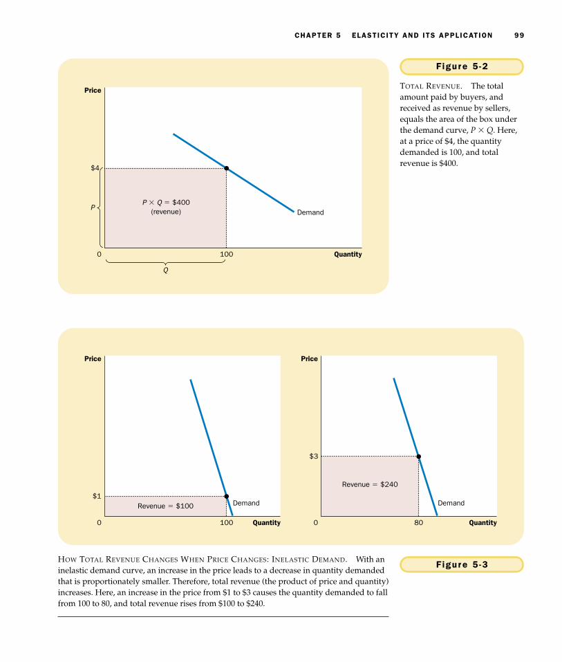
When studying changes in supply or demand in a market, one variable we oftenwant to study is total revenue, the amount paid by buyers and received by sellersof the good. In any market, total revenue is P � Q, the price of the good times thequantity of the good sold. We can show total revenue graphically, as in Figure 5-2.The height of the box under the demand curve is P, and the width is Q. The areaof this box, P � Q, equals the total revenue in this market. In Figure 5-2, whereP � $4 and Q � 100, total revenue is $4 � 100, or $400.

How does total revenue change as one moves along the demand curve? Theanswer depends on the price elasticity of demand. If demand is inelastic, as in Fig-ure 5-3, then an increase in the price causes an increase in total revenue. Here anincrease in price from $1 to $3 causes the quantity demanded to fall only from 100

tota l r evenuethe amount paid by buyers andreceived by sellers of a good,computed as the price of the goodtimes the quantity sold

(a) Perfectly Inelastic Demand: Elasticity Equals 0

$5

4

Demand

Quantity1000

(b) Inelastic Demand: Elasticity Is Less Than 1

$5

4

Quantity1000 90

Demand

(c) Unit Elastic Demand: Elasticity Equals 1

$5

4

Demand

Quantity1000

Price

80

1. Anincreasein price . . .

2. . . . leaves the quantity demanded unchanged.

2. . . . leads to a 22% decrease in quantity demanded.

1. A 22%increasein price . . .

Price Price

2. . . . leads to an 11% decrease in quantity demanded.


(d) Elastic Demand: Elasticity Is Greater Than 1

$5

4 Demand

Quantity1000

Price

50

(e) Perfectly Elastic Demand: Elasticity Equals Infinity

$4

Quantity0

Price

Demand


2. At exactly $4,consumers willbuy any quantity.

1. At any priceabove $4, quantitydemanded is zero.

2. . . . leads to a 67% decrease in quantity demanded.3. At a price below $4,quantity demanded is infinite.

Figure 5 -1 THE PRICE ELASTICITY OF DEMAND. The price elasticity of demand determines whetherthe demand curve is steep or flat. Note that all percentage changes are calculated usingthe midpoint method.


$4

Demand

Quantity

Q

P

0

Price

P � Q � $400(revenue)

100

Figure 5 -2

TOTAL REVENUE. The totalamount paid by buyers, andreceived as revenue by sellers,equals the area of the box underthe demand curve, P � Q. Here,at a price of $4, the quantitydemanded is 100, and totalrevenue is $400.

$1Demand

Quantity0

Price

Revenue � $100

100

$3

Quantity0

Price

80

Revenue � $240

Demand

Figure 5 -3HOW TOTAL REVENUE CHANGES WHEN PRICE CHANGES: INELASTIC DEMAND. With aninelastic demand curve, an increase in the price leads to a decrease in quantity demandedthat is proportionately smaller. Therefore, total revenue (the product of price and quantity)increases. Here, an increase in the price from $1 to $3 causes the quantity demanded to fallfrom 100 to 80, and total revenue rises from $100 to $240.


to 80, and so total revenue rises from $100 to $240. An increase in price raisesP � Q because the fall in Q is proportionately smaller than the rise in P.

We obtain the opposite result if demand is elastic: An increase in the pricecauses a decrease in total revenue. In Figure 5-4, for instance, when the price risesfrom $4 to $5, the quantity demanded falls from 50 to 20, and so total revenue fallsfrom $200 to $100. Because demand is elastic, the reduction in the quantity de-manded is so great that it more than offsets the increase in the price. That is, an in-crease in price reduces P � Q because the fall in Q is proportionately greater thanthe rise in P.

Although the examples in these two figures are extreme, they illustrate a gen-eral rule:

◆ When a demand curve is inelastic (a price elasticity less than 1), a priceincrease raises total revenue, and a price decrease reduces total revenue.

◆ When a demand curve is elastic (a price elasticity greater than 1), a priceincrease reduces total revenue, and a price decrease raises total revenue.

◆ In the special case of unit elastic demand (a price elasticity exactly equalto 1), a change in the price does not affect total revenue.

Demand

Quantity0

Price

Revenue � $200

$4

50

Demand

Quantity0

Price

Revenue � $100

$5

20

Figure 5 -4 HOW TOTAL REVENUE CHANGES WHEN PRICE CHANGES: ELASTIC DEMAND. With anelastic demand curve, an increase in the price leads to a decrease in quantity demandedthat is proportionately larger. Therefore, total revenue (the product of price and quantity)decreases. Here, an increase in the price from $4 to $5 causes the quantity demanded tofall from 50 to 20, so total revenue falls from $200 to $100.


CASE STUDY PRICING ADMISSION TO A MUSEUM

You are curator of a major art museum. Your director of finance tells you thatthe museum is running short of funds and suggests that you consider changing

ELASTICITY AND TOTAL REVENUE ALONGA LINEAR DEMAND CURVE

Although some demand curves have an elasticity that is the same along the entirecurve, that is not always the case. An example of a demand curve along whichelasticity changes is a straight line, as shown in Figure 5-5. A linear demand curvehas a constant slope. Recall that slope is defined as “rise over run,” which here isthe ratio of the change in price (“rise”) to the change in quantity (“run”). This par-ticular demand curve’s slope is constant because each $1 increase in price causesthe same 2-unit decrease in the quantity demanded.

Even though the slope of a linear demand curve is constant, the elasticity isnot. The reason is that the slope is the ratio of changes in the two variables, whereasthe elasticity is the ratio of percentage changes in the two variables. You can see thismost easily by looking at Table 5-1. This table shows the demand schedule for thelinear demand curve in Figure 5-5 and calculates the price elasticity of demandusing the midpoint method discussed earlier. At points with low price and highquantity, the demand curve is inelastic. At points with a high price and low quan-tity, the demand curve is elastic.

Table 5-1 also presents total revenue at each point on the demand curve. Thesenumbers illustrate the relationship between total revenue and elasticity. When theprice is $1, for instance, demand is inelastic, and a price increase to $2 raises totalrevenue. When the price is $5, demand is elastic, and a price increase to $6 reducestotal revenue. Between $3 and $4, demand is exactly unit elastic, and total revenueis the same at these two prices.

5

6

$7

4

1

2

3

Quantity122 4 6 8 10 140

PriceElasticity islargerthan 1.

Elasticity issmallerthan 1.

Figure5 -5

A LINEAR DEMAND CURVE.The slope of a linear demandcurve is constant, but its elasticityis not.


the price of admission to increase total revenue. What do you do? Do you raisethe price of admission, or do you lower it?

The answer depends on the elasticity of demand. If the demand for visits tothe museum is inelastic, then an increase in the price of admission would in-crease total revenue. But if the demand is elastic, then an increase in pricewould cause the number of visitors to fall by so much that total revenue woulddecrease. In this case, you should cut the price. The number of visitors wouldrise by so much that total revenue would increase.

To estimate the price elasticity of demand, you would need to turn to yourstatisticians. They might use historical data to study how museum attendancevaried from year to year as the admission price changed. Or they might usedata on attendance at the various museums around the country to see how theadmission price affects attendance. In studying either of these sets of data, thestatisticians would need to take account of other factors that affect attendance—weather, population, size of collection, and so forth—in order to isolate the ef-fect of price. In the end, such data analysis would provide an estimate of theprice elasticity of demand, which you could use in deciding how to respond toyour financial problem.

OTHER DEMAND ELASTICIT IES

In addition to the price elasticity of demand, economists also use other elasticitiesto describe the behavior of buyers in a market.

The Income E last ic i ty o f Demand Economists use the income elas-ticity of demand to measure how the quantity demanded changes as consumer in-come changes. The income elasticity is the percentage change in quantitydemanded divided by the percentage change in income. That is,

Table 5 -1

TOTAL

REVENUE PERCENT PERCENT

(PRICE � CHANGE IN CHANGE IN

PRICE QUANTITY QUANTITY) PRICE QUANTITY ELASTICITY DESCRIPTION

$7 0 $ 015 200 13.0 Elastic

6 2 1218 67 3.7 Elastic

5 4 2022 40 1.8 Elastic

4 6 2429 29 1.0 Unit elastic

3 8 2440 22 0.6 Inelastic

2 10 2067 18 0.3 Inelastic

1 12 12200 15 0.1 Inelastic

0 14 0

COMPUTING THE ELASTICITY OF A LINEAR DEMAND CURVE

NOTE: Elasticity is calculated here using the midpoint method.

IF THE PRICE OF ADMISSION WERE HIGHER,HOW MUCH SHORTER WOULD THIS LINE

BECOME?

income e last ic i ty o fdemanda measure of how much the quantitydemanded of a good responds to achange in consumers’ income,computed as the percentage changein quantity demanded divided by thepercentage change in income


Income elasticity of demand � .

As we discussed in Chapter 4, most goods are normal goods: Higher income raisesquantity demanded. Because quantity demanded and income move in the samedirection, normal goods have positive income elasticities. A few goods, such as bus

Percentage change in quantity demandedPercentage change in income

HOW SHOULD A FIRM THAT OPERATES A

private toll road set a price for its ser-vice? As the following article makesclear, answering this question requiresan understanding of the demand curveand its elasticity.

F o r W h o m t h e B o o t h To l l s ,P r i c e R e a l l y D o e s M a t t e r

BY STEVEN PEARLSTEIN

All businesses face a similar question:What price for their product will generatethe maximum profit?

The answer is not always obvious:Raising the price of something often hasthe effect of reducing sales as price-sensitive consumers seek alternatives orsimply do without. For every product, theextent of that sensitivity is different. Thetrick is to find the point for each wherethe ideal tradeoff between profit marginand sales volume is achieved.

Right now, the developers of a newprivate toll road between Leesburg and

Washington-Dulles International Airportare trying to discern the magic point. Thegroup originally projected that it couldcharge nearly $2 for the 14-mile one-waytrip, while attracting 34,000 trips on anaverage day from overcrowded publicroads such as nearby Route 7. But afterspending $350 million to build their muchheralded “Greenway,” they discoveredto their dismay that only about a thirdthat number of commuters were willingto pay that much to shave 20 minutes offtheir daily commute. . . .

It was only when the company, indesperation, lowered the toll to $1 that itcame even close to attracting the ex-pected traffic flows.

Although the Greenway still is los-ing money, it is clearly better off at thisnew point on the demand curve than itwas when it first opened. Average dailyrevenue today is $22,000, comparedwith $14,875 when the “special intro-ductory” price was $1.75. And with traf-fic still light even at rush hour, it ispossible that the owners may lower tollseven further in search of higher revenue.

After all, when the price was low-ered by 45 percent last spring, it gener-ated a 200 percent increase in volumethree months later. If the same ratio ap-plies again, lowering the toll another25 percent would drive the daily volumeup to 38,000 trips, and daily revenue upto nearly $29,000.

The problem, of course, is that thesame ratio usually does not apply at

every price point, which is why this pric-ing business is so tricky. . . .

Clifford Winston of the BrookingsInstitution and John Calfee of the Ameri-can Enterprise Institute have consideredthe toll road’s dilemma. . . .

Last year, the economists con-ducted an elaborate market test with1,170 people across the country whowere each presented with a series of op-tions in which they were, in effect, askedto make a personal tradeoff betweenless commuting time and higher tolls.

In the end, they concluded that thepeople who placed the highest value onreducing their commuting time alreadyhad done so by finding public transporta-tion, living closer to their work, or select-ing jobs that allowed them to commuteat off-peak hours.

Conversely, those who commutedsignificant distances had a higher toler-ance for traffic congestion and were will-ing to pay only 20 percent of their hourlypay to save an hour of their time.

Overall, the Winston/Calfee find-ings help explain why the Greenway’soriginal toll and volume projections weretoo high: By their reckoning, only com-muters who earned at least $30 an hour(about $60,000 a year) would be willingto pay $2 to save 20 minutes.

SOURCE: The Washington Post, October 24, 1996,p. E1.

IN THE NEWS

On the Roadwith Elasticity


rides, are inferior goods: Higher income lowers the quantity demanded. Becausequantity demanded and income move in opposite directions, inferior goods havenegative income elasticities.

Even among normal goods, income elasticities vary substantially in size. Ne-cessities, such as food and clothing, tend to have small income elasticities becauseconsumers, regardless of how low their incomes, choose to buy some of thesegoods. Luxuries, such as caviar and furs, tend to have large income elasticities be-cause consumers feel that they can do without these goods altogether if their in-come is too low.

The Cross -P r ice E last ic i ty o f Demand Economists use the cross-price elasticity of demand to measure how the quantity demanded of one goodchanges as the price of another good changes. It is calculated as the percentagechange in quantity demanded of good 1 divided by the percentage change in theprice of good 2. That is,

Cross-price elasticity of demand � .

Whether the cross-price elasticity is a positive or negative number depends onwhether the two goods are substitutes or complements. As we discussed in Chap-ter 4, substitutes are goods that are typically used in place of one another, such ashamburgers and hot dogs. An increase in hot dog prices induces people to grillhamburgers instead. Because the price of hot dogs and the quantity of hamburgersdemanded move in the same direction, the cross-price elasticity is positive. Con-versely, complements are goods that are typically used together, such as comput-ers and software. In this case, the cross-price elasticity is negative, indicating thatan increase in the price of computers reduces the quantity of software demanded.

QUICK QUIZ: Define the price elasticity of demand. ◆ Explain the relationship between total revenue and the price elasticity of demand.

THE ELASTICITY OF SUPPLY

When we discussed the determinants of supply in Chapter 4, we noted that sellersof a good increase the quantity supplied when the price of the good rises, whentheir input prices fall, or when their technology improves. To turn from qualita-tive to quantitative statements about supply, we once again use the concept ofelasticity.

THE PRICE ELASTICITY OF SUPPLYAND ITS DETERMINANTS

The law of supply states that higher prices raise the quantity supplied. The priceelasticity of supply measures how much the quantity supplied responds tochanges in the price. Supply of a good is said to be elastic if the quantity supplied

Percentage change in quantitydemanded of good 1Percentage change in

the price of good 2

cross -p r ice e last ic i ty o fdemanda measure of how much the quantitydemanded of one good responds to achange in the price of another good,computed as the percentage changein quantity demanded of the firstgood divided by the percentagechange in the price of the secondgood

pr ice e last ic i ty o f supp lya measure of how much the quantitysupplied of a good responds to achange in the price of that good,computed as the percentage changein quantity supplied divided by thepercentage change in price


responds substantially to changes in the price. Supply is said to be inelastic if thequantity supplied responds only slightly to changes in the price.

The price elasticity of supply depends on the flexibility of sellers to change theamount of the good they produce. For example, beachfront land has an inelasticsupply because it is almost impossible to produce more of it. By contrast, manu-factured goods, such as books, cars, and televisions, have elastic supplies becausethe firms that produce them can run their factories longer in response to a higherprice.

In most markets, a key determinant of the price elasticity of supply is the timeperiod being considered. Supply is usually more elastic in the long run than in theshort run. Over short periods of time, firms cannot easily change the size of theirfactories to make more or less of a good. Thus, in the short run, the quantity sup-plied is not very responsive to the price. By contrast, over longer periods, firms canbuild new factories or close old ones. In addition, new firms can enter a market,and old firms can shut down. Thus, in the long run, the quantity supplied can re-spond substantially to the price.

COMPUTING THE PRICE ELASTICITY OF SUPPLY

Now that we have some idea about what the price elasticity of supply is, let’s bemore precise. Economists compute the price elasticity of supply as the percentagechange in the quantity supplied divided by the percentage change in the price.That is,

Price elasticity of supply � .

For example, suppose that an increase in the price of milk from $2.85 to $3.15 a gal-lon raises the amount that dairy farmers produce from 9,000 to 11,000 gallons permonth. Using the midpoint method, we calculate the percentage change in price as

Percentage change in price � (3.15 � 2.85)/3.00 � 100 � 10 percent.

Similarly, we calculate the percentage change in quantity supplied as

Percentage change in quantity supplied � (11,000 � 9,000)/10,000 � 100� 20 percent.

In this case, the price elasticity of supply is

Price elasticity of supply � � 2.0.

In this example, the elasticity of 2 reflects the fact that the quantity supplied movesproportionately twice as much as the price.

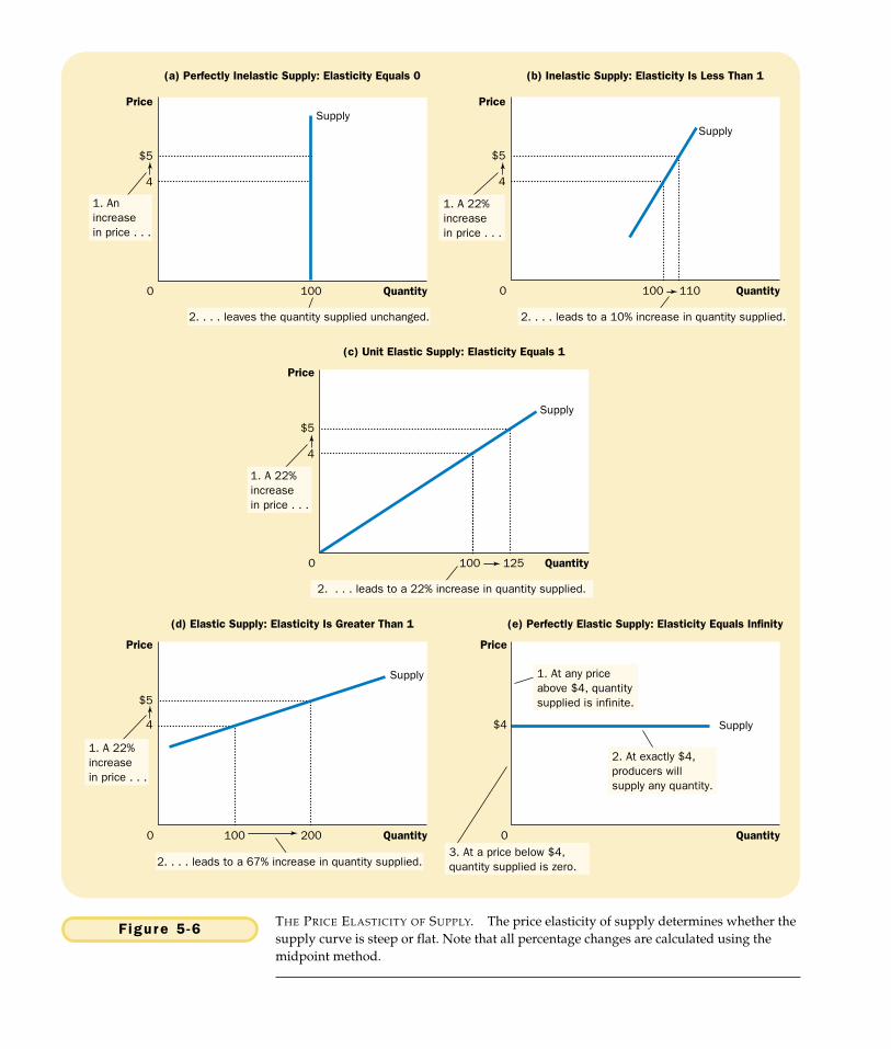
THE VARIETY OF SUPPLY CURVES

Because the price elasticity of supply measures the responsiveness of quantity sup-plied to the price, it is reflected in the appearance of the supply curve. Figure 5-6shows five cases. In the extreme case of a zero elasticity, supply is perfectly inelastic,

20 percent10 percent

Percentage change in quantity suppliedPercentage change in price

100 110

100 125

(a) Perfectly Inelastic Supply: Elasticity Equals 0

$5

4

Supply

Quantity1000

(b) Inelastic Supply: Elasticity Is Less Than 1

$5

4

Quantity0

(c) Unit Elastic Supply: Elasticity Equals 1

$5

4

Quantity0

Price

1. Anincreasein price . . .

2. . . . leaves the quantity supplied unchanged.

2. . . . leads to a 22% increase in quantity supplied.


Price Price

2. . . . leads to a 10% increase in quantity supplied.


(d) Elastic Supply: Elasticity Is Greater Than 1

$5

4

Quantity0

Price

(e) Perfectly Elastic Supply: Elasticity Equals Infinity

$4

Quantity0

Price

Supply


2. At exactly $4,producers willsupply any quantity.

1. At any priceabove $4, quantitysupplied is infinite.

2. . . . leads to a 67% increase in quantity supplied.3. At a price below $4,quantity supplied is zero.

Supply

Supply

100 200

Supply

Figure 5 -6 THE PRICE ELASTICITY OF SUPPLY. The price elasticity of supply determines whether thesupply curve is steep or flat. Note that all percentage changes are calculated using themidpoint method.


and the supply curve is vertical. In this case, the quantity supplied is the same re-gardless of the price. As the elasticity rises, the supply curve gets flatter, whichshows that the quantity supplied responds more to changes in the price. At the op-posite extreme, supply is perfectly elastic. This occurs as the price elasticity of sup-ply approaches infinity and the supply curve becomes horizontal, meaning thatvery small changes in the price lead to very large changes in the quantity supplied.

In some markets, the elasticity of supply is not constant but varies over thesupply curve. Figure 5-7 shows a typical case for an industry in which firms havefactories with a limited capacity for production. For low levels of quantity sup-plied, the elasticity of supply is high, indicating that firms respond substantially tochanges in the price. In this region, firms have capacity for production that is notbeing used, such as plants and equipment sitting idle for all or part of the day.Small increases in price make it profitable for firms to begin using this idle capac-ity. As the quantity supplied rises, firms begin to reach capacity. Once capacity isfully used, increasing production further requires the construction of new plants.To induce firms to incur this extra expense, the price must rise substantially, sosupply becomes less elastic.

Figure 5-7 presents a numerical example of this phenomenon. When the pricerises from $3 to $4 (a 29 percent increase, according to the midpoint method), thequantity supplied rises from 100 to 200 (a 67 percent increase). Because quantitysupplied moves proportionately more than the price, the supply curve has elastic-ity greater than 1. By contrast, when the price rises from $12 to $15 (a 22 percent in-crease), the quantity supplied rises from 500 to 525 (a 5 percent increase). In thiscase, quantity supplied moves proportionately less than the price, so the elasticityis less than 1.

QUICK QUIZ: Define the price elasticity of supply. ◆ Explain why the the price elasticity of supply might be different in the long run than in the short run.

$15

12

3

Quantity100 200 5000

Price

525

Elasticity is small(less than 1).

Elasticity is large(greater than 1).

4

Figure 5 -7

HOW THE PRICE ELASTICITY OF

SUPPLY CAN VARY. Becausefirms often have a maximumcapacity for production, theelasticity of supply may be veryhigh at low levels of quantitysupplied and very low at highlevels of quantity supplied. Here,an increase in price from $3 to $4increases the quantity suppliedfrom 100 to 200. Because theincrease in quantity supplied of100 percent is larger than theincrease in price of 33 percent, thesupply curve is elastic in thisrange. By contrast, when theprice rises from $12 to $15, thequantity supplied rises only from500 to 525. Because the increase inquantity supplied of 5 percent issmaller than the increase in priceof 25 percent, the supply curve isinelastic in this range.


THREE APPLICATIONS OF SUPPLY,DEMAND, AND ELASTICITY

Can good news for farming be bad news for farmers? Why did the Organization ofPetroleum Exporting Countries (OPEC) fail to keep the price of oil high? Doesdrug interdiction increase or decrease drug-related crime? At first, these questionsmight seem to have little in common. Yet all three questions are about markets,and all markets are subject to the forces of supply and demand. Here we apply theversatile tools of supply, demand, and elasticity to answer these seemingly com-plex questions.

CAN GOOD NEWS FOR FARMING BEBAD NEWS FOR FARMERS?

Let’s now return to the question posed at the beginning of this chapter: What hap-pens to wheat farmers and the market for wheat when university agronomists dis-cover a new wheat hybrid that is more productive than existing varieties? Recallfrom Chapter 4 that we answer such questions in three steps. First, we examinewhether the supply curve or demand curve shifts. Second, we consider which di-rection the curve shifts. Third, we use the supply-and-demand diagram to see howthe market equilibrium changes.

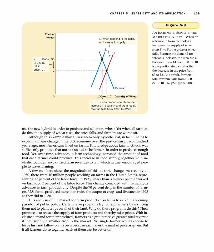
In this case, the discovery of the new hybrid affects the supply curve. Becausethe hybrid increases the amount of wheat that can be produced on each acre ofland, farmers are now willing to supply more wheat at any given price. In otherwords, the supply curve shifts to the right. The demand curve remains the samebecause consumers’ desire to buy wheat products at any given price is not affectedby the introduction of a new hybrid. Figure 5-8 shows an example of such achange. When the supply curve shifts from S1 to S2, the quantity of wheat sold in-creases from 100 to 110, and the price of wheat falls from $3 to $2.

But does this discovery make farmers better off? As a first cut to answeringthis question, consider what happens to the total revenue received by farmers.Farmers’ total revenue is P � Q, the price of the wheat times the quantity sold. Thediscovery affects farmers in two conflicting ways. The hybrid allows farmers toproduce more wheat (Q rises), but now each bushel of wheat sells for less (P falls).

Whether total revenue rises or falls depends on the elasticity of demand. Inpractice, the demand for basic foodstuffs such as wheat is usually inelastic, forthese items are relatively inexpensive and have few good substitutes. When thedemand curve is inelastic, as it is in Figure 5-8, a decrease in price causes total rev-enue to fall. You can see this in the figure: The price of wheat falls substantially,whereas the quantity of wheat sold rises only slightly. Total revenue falls from$300 to $220. Thus, the discovery of the new hybrid lowers the total revenue thatfarmers receive for the sale of their crops.

If farmers are made worse off by the discovery of this new hybrid, why dothey adopt it? The answer to this question goes to the heart of how competitivemarkets work. Because each farmer is a small part of the market for wheat, he orshe takes the price of wheat as given. For any given price of wheat, it is better to


use the new hybrid in order to produce and sell more wheat. Yet when all farmersdo this, the supply of wheat rises, the price falls, and farmers are worse off.

Although this example may at first seem only hypothetical, in fact it helps toexplain a major change in the U.S. economy over the past century. Two hundredyears ago, most Americans lived on farms. Knowledge about farm methods wassufficiently primitive that most of us had to be farmers in order to produce enoughfood. Yet, over time, advances in farm technology increased the amount of foodthat each farmer could produce. This increase in food supply, together with in-elastic food demand, caused farm revenues to fall, which in turn encouraged peo-ple to leave farming.

A few numbers show the magnitude of this historic change. As recently as1950, there were 10 million people working on farms in the United States, repre-senting 17 percent of the labor force. In 1998, fewer than 3 million people workedon farms, or 2 percent of the labor force. This change coincided with tremendousadvances in farm productivity: Despite the 70 percent drop in the number of farm-ers, U.S. farms produced more than twice the output of crops and livestock in 1998as they did in 1950.

This analysis of the market for farm products also helps to explain a seemingparadox of public policy: Certain farm programs try to help farmers by inducingthem not to plant crops on all of their land. Why do these programs do this? Theirpurpose is to reduce the supply of farm products and thereby raise prices. With in-elastic demand for their products, farmers as a group receive greater total revenueif they supply a smaller crop to the market. No single farmer would choose toleave his land fallow on his own because each takes the market price as given. Butif all farmers do so together, each of them can be better off.

$3

2

Quantity of Wheat1000

Price ofWheat 1. When demand is inelastic,

an increase in supply . . .

3. . . . and a proportionately smallerincrease in quantity sold. As a result,revenue falls from $300 to $220.

110

Demand

S1S2

2. . . . leadsto a largefall inprice . . .

Figure 5 -8

AN INCREASE IN SUPPLY IN THE

MARKET FOR WHEAT. When anadvance in farm technologyincreases the supply of wheatfrom S1 to S2, the price of wheatfalls. Because the demand forwheat is inelastic, the increase inthe quantity sold from 100 to 110is proportionately smaller thanthe decrease in the price from$3 to $2. As a result, farmers’total revenue falls from $300($3 � 100) to $220 ($2 � 110).


When analyzing the effects of farm technology or farm policy, it is importantto keep in mind that what is good for farmers is not necessarily good for society asa whole. Improvement in farm technology can be bad for farmers who become in-creasingly unnecessary, but it is surely good for consumers who pay less for food.Similarly, a policy aimed at reducing the supply of farm products may raise the in-comes of farmers, but it does so at the expense of consumers.

WHY DID OPEC FAIL TO KEEP THE PRICE OF OIL HIGH?

Many of the most disruptive events for the world’s economies over the past sev-eral decades have originated in the world market for oil. In the 1970s members ofthe Organization of Petroleum Exporting Countries (OPEC) decided to raise theworld price of oil in order to increase their incomes. These countries accomplishedthis goal by jointly reducing the amount of oil they supplied. From 1973 to 1974,the price of oil (adjusted for overall inflation) rose more than 50 percent. Then, afew years later, OPEC did the same thing again. The price of oil rose 14 percent in1979, followed by 34 percent in 1980, and another 34 percent in 1981.

Yet OPEC found it difficult to maintain a high price. From 1982 to 1985, theprice of oil steadily declined at about 10 percent per year. Dissatisfaction and dis-array soon prevailed among the OPEC countries. In 1986 cooperation amongOPEC members completely broke down, and the price of oil plunged 45 percent.In 1990 the price of oil (adjusted for overall inflation) was back to where it beganin 1970, and it has stayed at that low level throughout most of the 1990s.

This episode shows how supply and demand can behave differently in theshort run and in the long run. In the short run, both the supply and demand for oilare relatively inelastic. Supply is inelastic because the quantity of known oil re-serves and the capacity for oil extraction cannot be changed quickly. Demand is in-elastic because buying habits do not respond immediately to changes in price.Many drivers with old gas-guzzling cars, for instance, will just pay the higher


price. Thus, as panel (a) of Figure 5-9 shows, the short-run supply and demandcurves are steep. When the supply of oil shifts from S1 to S2, the price increase fromP1 to P2 is large.

The situation is very different in the long run. Over long periods of time, pro-ducers of oil outside of OPEC respond to high prices by increasing oil explorationand by building new extraction capacity. Consumers respond with greater conser-vation, for instance by replacing old inefficient cars with newer efficient ones.Thus, as panel (b) of Figure 5-9 shows, the long-run supply and demand curves aremore elastic. In the long run, the shift in the supply curve from S1 to S2 causes amuch smaller increase in the price.

This analysis shows why OPEC succeeded in maintaining a high price of oilonly in the short run. When OPEC countries agreed to reduce their production ofoil, they shifted the supply curve to the left. Even though each OPEC member soldless oil, the price rose by so much in the short run that OPEC incomes rose. By con-trast, in the long run when supply and demand are more elastic, the same reduc-tion in supply, measured by the horizontal shift in the supply curve, caused asmaller increase in the price. Thus, OPEC’s coordinated reduction in supplyproved less profitable in the long run.

OPEC still exists today. You will occasionally hear in the news about meetingsof officials from the OPEC countries. Cooperation among OPEC countries is less

P2

P1

Quantity of Oil0

Price of Oil

Demand

S2S1

(a) The Oil Market in the Short Run

P2

P1

Quantity of Oil0

Price of Oil

Demand

S2

S1

(b) The Oil Market in the Long Run

2. . . . leadsto a largeincreasein price.

1. In the long run,when supply anddemand are elastic,a shift in supply . . .

2. . . . leadsto a smallincreasein price.

1. In the short run, when supplyand demand are inelastic,a shift in supply . . .

Figure 5 -9A REDUCTION IN SUPPLY IN THE WORLD MARKET FOR OIL. When the supply of oil falls,the response depends on the time horizon. In the short run, supply and demand arerelatively inelastic, as in panel (a). Thus, when the supply curve shifts from S1 to S2, theprice rises substantially. By contrast, in the long run, supply and demand are relativelyelastic, as in panel (b). In this case, the same size shift in the supply curve (S1 to S2) causesa smaller increase in the price.


common now, however, in part because of the organization’s past failure at main-taining a high price.

DOES DRUG INTERDICTION INCREASEOR DECREASE DRUG-RELATED CRIME?

A persistent problem facing our society is the use of illegal drugs, such as heroin,cocaine, and crack. Drug use has several adverse effects. One is that drug depen-dency can ruin the lives of drug users and their families. Another is that drugaddicts often turn to robbery and other violent crimes to obtain the money neededto support their habit. To discourage the use of illegal drugs, the U.S. govern-ment devotes billions of dollars each year to reduce the flow of drugs into thecountry. Let’s use the tools of supply and demand to examine this policy of druginterdiction.

Suppose the government increases the number of federal agents devoted tothe war on drugs. What happens in the market for illegal drugs? As is usual, weanswer this question in three steps. First, we consider whether the supply curve ordemand curve shifts. Second, we consider the direction of the shift. Third, we seehow the shift affects the equilibrium price and quantity.

Although the purpose of drug interdiction is to reduce drug use, its direct im-pact is on the sellers of drugs rather than the buyers. When the government stopssome drugs from entering the country and arrests more smugglers, it raises thecost of selling drugs and, therefore, reduces the quantity of drugs supplied at anygiven price. The demand for drugs—the amount buyers want at any given price—is not changed. As panel (a) of Figure 5-10 shows, interdiction shifts the supplycurve to the left from S1 to S2 and leaves the demand curve the same. The equilib-rium price of drugs rises from P1 to P2, and the equilibrium quantity falls from Q1

to Q2. The fall in the equilibrium quantity shows that drug interdiction does re-duce drug use.

But what about the amount of drug-related crime? To answer this question,consider the total amount that drug users pay for the drugs they buy. Because fewdrug addicts are likely to break their destructive habits in response to a higherprice, it is likely that the demand for drugs is inelastic, as it is drawn in the figure.If demand is inelastic, then an increase in price raises total revenue in the drugmarket. That is, because drug interdiction raises the price of drugs proportionatelymore than it reduces drug use, it raises the total amount of money that drug userspay for drugs. Addicts who already had to steal to support their habits wouldhave an even greater need for quick cash. Thus, drug interdiction could increasedrug-related crime.

Because of this adverse effect of drug interdiction, some analysts argue for al-ternative approaches to the drug problem. Rather than trying to reduce the supplyof drugs, policymakers might try to reduce the demand by pursuing a policy ofdrug education. Successful drug education has the effects shown in panel (b) ofFigure 5-10. The demand curve shifts to the left from D1 to D2. As a result, the equi-librium quantity falls from Q1 to Q2, and the equilibrium price falls from P1 to P2.Total revenue, which is price times quantity, also falls. Thus, in contrast to drug in-terdiction, drug education can reduce both drug use and drug-related crime.

Advocates of drug interdiction might argue that the effects of this policy aredifferent in the long run than in the short run, because the elasticity of demandmay depend on the time horizon. The demand for drugs is probably inelastic over


short periods of time because higher prices do not substantially affect drug use byestablished addicts. But demand may be more elastic over longer periods of timebecause higher prices would discourage experimentation with drugs among theyoung and, over time, lead to fewer drug addicts. In this case, drug interdic-tion would increase drug-related crime in the short run while decreasing it in thelong run.

QUICK QUIZ: How might a drought that destroys half of all farm crops be good for farmers? If such a drought is good for farmers, why don’t farmers destroy their own crops in the absence of a drought?

CONCLUSION

According to an old quip, even a parrot can become an economist simply by learn-ing to say “supply and demand.” These last two chapters should have convincedyou that there is much truth in this statement. The tools of supply and demandallow you to analyze many of the most important events and policies that shape

P2

P1

Quantity of Drugs0 Q2 Q1

Price ofDrugs

Demand

S2

S1

Q2 Q1

(a) Drug Interdiction

Quantity of Drugs0

Price ofDrugs

Supply

D2

D1

(b) Drug Education

3. . . . and reduces the quantity sold.

2. . . . whichraises theprice . . .

2. . . . whichreduces the price . . .

P1

P2

1. Drug interdiction reducesthe supply of drugs . . .

1. Drug education reducesthe demand for drugs . . .

3. . . . and reduces the quantity sold.

Figure 5 -10POLICIES TO REDUCE THE USE OF ILLEGAL DRUGS. Drug interdiction reduces the supplyof drugs from S1 to S2, as in panel (a). If the demand for drugs is inelastic, then the totalamount paid by drug users rises, even as the amount of drug use falls. By contrast, drugeducation reduces the demand for drugs from D1 to D2, as in panel (b). Because both priceand quantity fall, the amount paid by drug users falls.


the economy. You are now well on your way to becoming an economist (or, at least,a well-educated parrot).

◆ The price elasticity of demand measures how much thequantity demanded responds to changes in the price.Demand tends to be more elastic if the good is a luxuryrather than a necessity, if close substitutes are available,if the market is narrowly defined, or if buyers havesubstantial time to react to a price change.

◆ The price elasticity of demand is calculated as thepercentage change in quantity demanded divided bythe percentage change in price. If the elasticity is lessthan 1, so that quantity demanded movesproportionately less than the price, demand is said to beinelastic. If the elasticity is greater than 1, so thatquantity demanded moves proportionately more thanthe price, demand is said to be elastic.

◆ Total revenue, the total amount paid for a good, equalsthe price of the good times the quantity sold. Forinelastic demand curves, total revenue rises as pricerises. For elastic demand curves, total revenue falls asprice rises.

◆ The income elasticity of demand measures how muchthe quantity demanded responds to changes in

consumers’ income. The cross-price elasticity of demandmeasures how much the quantity demanded of onegood responds to the price of another good.

◆ The price elasticity of supply measures how much thequantity supplied responds to changes in the price. Thiselasticity often depends on the time horizon underconsideration. In most markets, supply is more elastic inthe long run than in the short run.

◆ The price elasticity of supply is calculated as thepercentage change in quantity supplied divided by thepercentage change in price. If the elasticity is less than 1,so that quantity supplied moves proportionately lessthan the price, supply is said to be inelastic. If theelasticity is greater than 1, so that quantity suppliedmoves proportionately more than the price, supply issaid to be elastic.

◆ The tools of supply and demand can be applied in manydifferent kinds of markets. This chapter uses them toanalyze the market for wheat, the market for oil, and themarket for illegal drugs.

Summar y

elasticity, p. xxxprice elasticity of demand, p. xxx

total revenue, p. xxxincome elasticity of demand, p. xxx

cross-price elasticity of demand, p. xxxprice elasticity of supply, p. xxx

Key Concepts

1. Define the price elasticity of demand and the incomeelasticity of demand.

2. List and explain some of the determinants of the priceelasticity of demand.

3. If the elasticity is greater than 1, is demand elastic orinelastic? If the elasticity equals 0, is demand perfectlyelastic or perfectly inelastic?

4. On a supply-and-demand diagram, show equilibriumprice, equilibrium quantity, and the total revenuereceived by producers?

5. If demand is elastic, how will an increase in pricechange total revenue? Explain.

6. What do we call a good whose income elasticity is lessthan 0?

7. How is the price elasticity of supply calculated? Explainwhat this measures.

8. What is the price elasticity of supply of Picassopaintings?

9. Is the price elasticity of supply usually larger in theshort run or in the long run? Why?

10. In the 1970s, OPEC caused a dramatic increase in theprice of oil. What prevented it from maintaining thishigh price through the 1980s?

Quest ions fo r Rev iew


1. For each of the following pairs of goods, which goodwould you expect to have more elastic demandand why?a. required textbooks or mystery novelsb. Beethoven recordings or classical music recordings

in generalc. heating oil during the next six months or heating oil

during the next five yearsd. root beer or water

2. Suppose that business travelers and vacationers havethe following demand for airline tickets from New Yorkto Boston:

QUANTITY DEMANDED QUANTITY DEMANDED

PRICE (BUSINESS TRAVELERS) (VACATIONERS)

$150 2,100 1,000200 2,000 800250 1,900 600300 1,800 400

a. As the price of tickets rises from $200 to $250, whatis the price elasticity of demand for (i) businesstravelers and (ii) vacationers? (Use the midpointmethod in your calculations.)

b. Why might vacationers have a different elasticitythan business travelers?

3. Suppose that your demand schedule for compact discsis as follows:

QUANTITY DEMANDED QUANTITY DEMANDED

PRICE (INCOME � $10,000) (INCOME � $12,000)

$ 8 40 5010 32 4512 24 3014 16 2016 8 12

a. Use the midpoint method to calculate your priceelasticity of demand as the price of compact discsincreases from $8 to $10 if (i) your income is$10,000, and (ii) your income is $12,000.

b. Calculate your income elasticity of demand as yourincome increases from $10,000 to $12,000 if (i) theprice is $12, and (ii) the price is $16.

4. Emily has decided always to spend one-third of herincome on clothing.a. What is her income elasticity of clothing demand?

b. What is her price elasticity of clothing demand?c. If Emily’s tastes change and she decides to spend

only one-fourth of her income on clothing, howdoes her demand curve change? What are herincome elasticity and price elasticity now?

5. The New York Times reported (Feb. 17, 1996, p. 25) thatsubway ridership declined after a fare increase: “Therewere nearly four million fewer riders in December 1995,the first full month after the price of a token increased25 cents to $1.50, than in the previous December, a 4.3percent decline.”a. Use these data to estimate the price elasticity of

demand for subway rides.b. According to your estimate, what happens to the

Transit Authority’s revenue when the fare rises?c. Why might your estimate of the elasticity be

unreliable?

6. Two drivers—Tom and Jerry—each drive up to a gasstation. Before looking at the price, each places an order.Tom says, “I’d like 10 gallons of gas.” Jerry says, “I’dlike $10 of gas.” What is each driver’s price elasticity ofdemand?

7. Economists have observed that spending on restaurantmeals declines more during economic downturns thandoes spending on food to be eaten at home. How mightthe concept of elasticity help to explain thisphenomenon?

8. Consider public policy aimed at smoking.a. Studies indicate that the price elasticity of demand

for cigarettes is about 0.4. If a pack of cigarettescurrently costs $2 and the government wants toreduce smoking by 20 percent, by how muchshould it increase the price?

b. If the government permanently increases theprice of cigarettes, will the policy have a largereffect on smoking one year from now or five yearsfrom now?

c. Studies also find that teenagers have a higher priceelasticity than do adults. Why might this be true?

9. Would you expect the price elasticity of demand to belarger in the market for all ice cream or the market forvanilla ice cream? Would you expect the price elasticityof supply to be larger in the market for all ice cream orthe market for vanilla ice cream? Be sure to explain youranswers.

10. Pharmaceutical drugs have an inelastic demand, andcomputers have an elastic demand. Suppose that

Prob lems and App l icat ions


technological advance doubles the supply of bothproducts (that is, the quantity supplied at each price istwice what it was).a. What happens to the equilibrium price and

quantity in each market?b. Which product experiences a larger change in

price?c. Which product experiences a larger change in

quantity?d. What happens to total consumer spending on each

product?

11. Beachfront resorts have an inelastic supply, andautomobiles have an elastic supply. Suppose that a risein population doubles the demand for both products(that is, the quantity demanded at each price is twicewhat it was).a. What happens to the equilibrium price and

quantity in each market?b. Which product experiences a larger change in

price?c. Which product experiences a larger change in

quantity?d. What happens to total consumer spending on each

product?

12. Several years ago, flooding along the Missouri andMississippi rivers destroyed thousands of acres ofwheat.

a. Farmers whose crops were destroyed by the floodswere much worse off, but farmers whose cropswere not destroyed benefited from the floods.Why?

b. What information would you need about themarket for wheat in order to assess whetherfarmers as a group were hurt or helped by thefloods?

13. Explain why the following might be true: A droughtaround the world raises the total revenue that farmersreceive from the sale of grain, but a drought only inKansas reduces the total revenue that Kansas farmersreceive.

14. Because better weather makes farmland moreproductive, farmland in regions with good weatherconditions is more expensive than farmland in regionswith bad weather conditions. Over time, however, asadvances in technology have made all farmland moreproductive, the price of farmland (adjusted for overallinflation) has fallen. Use the concept of elasticity toexplain why productivity and farmland prices arepositively related across space but negatively relatedover time.

Eco 1

Documents

Transcript of Eco 1